microsoft excel 2007 basics for windows - information...

Copyright © 2009 by Massachusetts Institute of Technology All Rights Reserved Printed on 12/8/09

Microsoft Excel 2007 Basics

For Windows

Microsoft Excel 2007 Basics for Windows

Copyright © 2009 Massachusetts Institute of Technology All Rights Reserved 2 of 41

Table of Contents

Table of Contents ......................................................................................................................................................... 2

Module 1 – Getting Started ........................................................................................................................................ 5

Starting Microsoft Excel ........................................................................................................................................... 5

Creating and Opening Workbooks ........................................................................................................................... 5 Creating a new workbook .................................................................................................................................... 5 Opening an existing workbook ............................................................................................................................ 6

Workbooks and Worksheets ...................................................................................................................................... 6

Elements of a Window .............................................................................................................................................. 7 Title Bar and Menu Bar ....................................................................................................................................... 7 Standard and Formatting Toolbars ....................................................................................................................... 9 Zoom Control ....................................................................................................................................................... 9 Active Cell ........................................................................................................................................................... 9 Cell Address ......................................................................................................................................................... 9 Horizontal and Vertical Scroll Bars ................................................................................................................... 10 Name Box and Formula Bar .............................................................................................................................. 10 Row and Column Headings ............................................................................................................................... 11 Sheet Tabs and Tab Scrolling Buttons ............................................................................................................... 11 Status Bar ........................................................................................................................................................... 12

Exercise - Module 1 ................................................................................................................................................... 13

Module 2 – Saving ..................................................................................................................................................... 14

Naming workbooks ................................................................................................................................................. 14

Saving an unnamed workbook ................................................................................................................................ 14

Saving an existing workbook .................................................................................................................................. 14

Saving a copy of a workbook .................................................................................................................................. 14

Saving a workbook to a new location ..................................................................................................................... 15

Saving a workbook with a new name and to a new location .................................................................................. 15

Exercise - Module 2 ................................................................................................................................................... 16

Module 3 – Entering and Editing ............................................................................................................................. 17

Entering Worksheet Data ....................................................................................................................................... 17 Enter numbers, text, a date, or a time ................................................................................................................. 17 Ready and Edit modes ........................................................................................................................................ 17 Enter and edit the same data on multiple worksheets ........................................................................................ 18 Enter the same data into several cells at once .................................................................................................... 18 Automatically fill in data based on adjacent cells .............................................................................................. 18


Create a Custom List .......................................................................................................................................... 19 Import an existing Custom List .......................................................................................................................... 19

Editing Worksheet Data .......................................................................................................................................... 19 Edit cell contents ................................................................................................................................................ 19 Cancel , undo or redo an entry ........................................................................................................................... 20 Clear contents, formats, or comments from cells ............................................................................................... 20

Exercise - Module 3 ................................................................................................................................................... 21

Module 4 – Selecting and Navigating ....................................................................................................................... 22

Selecting .................................................................................................................................................................. 22

Grouping Worksheets ............................................................................................................................................. 22

Navigating .............................................................................................................................................................. 23 Using the scroll bars [see page 9, Figure 7] ....................................................................................................... 23 Using the keyboard ............................................................................................................................................ 23

Exercise - Module 4 ................................................................................................................................................... 24

Module 5 - Creating Formulas ................................................................................................................................. 25

How formulas work ................................................................................................................................................. 25

How operators work ............................................................................................................................................... 25

Creating a simple formula ...................................................................................................................................... 25

Using functions ....................................................................................................................................................... 26

Automatically sum a range of cells ......................................................................................................... 27

Sum multiple rows and columns ............................................................................................................................. 27

Naming a cell or a range, or cells .......................................................................................................................... 27 To name a cell or a range: .................................................................................................................................. 27

Absolute versus relative values ............................................................................................................................... 28

Exercise - Module 5 ................................................................................................................................................... 30

Module 6 – Formatting ............................................................................................................................................. 31

Basic Worksheet Formatting .................................................................................................................................. 31

Applying Borders and Shading ............................................................................................................................... 31

Number Formatting ................................................................................................................................................ 31

AutoFormat ............................................................................................................................................................. 31

Using Styles ............................................................................................................................................................ 32

Format Painter ....................................................................................................................................................... 32 To apply the formatting to adjacent cells: .......................................................................................................... 32




To apply the formatting to non-adjacent cells: .................................................................................................. 32

Exercise – Module 6 ................................................................................................................................................... 33

Module 7 - Printing ................................................................................................................................................... 34

Before you print ...................................................................................................................................................... 34

Modify the layout of the printed worksheet ............................................................................................................. 34

Change the worksheet area that appears on a printed page .................................................................................. 34

Print Preview .......................................................................................................................................................... 34

Print the active sheets, a selected range, or an entire workbook ........................................................................... 34

Create custom headers and footers ........................................................................................................................ 35

Change the font in header and footer text .............................................................................................................. 36

Print titles ............................................................................................................................................................... 36

Rows to Repeat at Top of Each Worksheet Page .................................................................................................... 36

Columns to Repeat at Left of Each Worksheet Page .............................................................................................. 36

Page Break ............................................................................................................................................................. 36

Exercise – Module 7 ................................................................................................................................................... 38

Module 8 – Getting Help ........................................................................................................................................... 39

When you have a question ...................................................................................................................................... 39

Office Assistant tool ................................................................................................................................................ 39

Dialog Box Screen Tips .......................................................................................................................................... 39

Toolbar Screen Tips ................................................................................................................................................ 39

MIT Computing Help Desk ..................................................................................................................................... 39

MIT Excel User Group ........................................................................................................................................... 40

Exercise - Module 8 ................................................................................................................................................... 40


Module 1 – Getting Started

Starting Microsoft Excel

There are several ways to start Excel. Here are a few.

• Double-click the Excel program icon or an existing Excel worksheet.

Excel 2007 program icon • Choose Microsoft Excel from the Microsoft Office Manager.

• Click on the Windows XP Start button, choose Programs, MS Office, MS Excel

Start button

Creating and Opening Workbooks

Creating a new workbook 1) On the Office button menu, click New.

2) In the New Workbook dialog box, click Create. 3) It’s much faster to click on the New Workbook tool on the Quick Access toolbar.



Opening an existing workbook

1) Click the Open tool on the Quick Access toolbar. The Open dialog box appears.

2) In the “Open” dialog box, you can navigate through the drop-down list in the Look in section, or use the icons in the sidebar to get to a location.

3) Once you find the workbook, double-click on it to open.

Tip: To open a workbook you've used recently, click its name in the Recent Documents list of the Office button.

Workbooks and Worksheets In Microsoft Excel, a workbook is the file where you work and store your data. Because each workbook can contain many sheets, you can organize various kinds of related information in a single file. In other words, a workbook is a collection of worksheets.

Worksheets are for listing and analyzing data. You can enter and edit data one worksheet or on several worksheets simultaneously and perform calculations based on data from multiple worksheets. You can add chart sheets to chart your worksheet data, and modules to create and store macros for special tasks you want to perform in the workbook. The names of the sheets appear on tabs at the bottom of the workbook window. To move from sheet to sheet, you click the sheet tabs (e.g., Sheet1, Sheet2…) and the name of the active sheet is always highlighted and bold. You can rename the sheets, add and delete sheets, and move, copy or link sheets within a workbook or to another workbook. You can also group worksheets. Each Excel workbook by default has 3 worksheets, but you can change the default to a higher or lower number. Each sheet contains 1,048,576 rows and 16,384 columns – that’s over 17 billion cells! Later on you will learn how to navigate in a very large worksheet.

To understand the distinction between a workbook and worksheet, think of an Excel workbook as a book containing many chapters. Although the worksheets in a workbook look like only one page, they can contain many pages of data. Therefore, the sheets are more like individual chapters in a book.



Elements of a Window

Title Bar and Ribbon

The Title Bar is at the top of every window in Windows (Workbook and Application can reside on one title bar) and identifies the name of the program (in this case, Microsoft Excel) and/or workbook (e.g., Book1). If your window is not maximized, you click and hold the left mouse button while dragging the title bar to move the window to a different location. The Office Button is located on the top left section of the Title Bar and Ribbon. From the Office Button you can select the appropriate command, such as choosing New, Open, Save, Print, and Close.

Note: that each menu item has one character underlined. This is so that you can use the keyboard rather than the mouse to access menus and menu commands. By pressing the [Alt] key, you place Excel in a keyboard mode, and you would be able to type the specified letter of a menu and menu command. For example, if you wanted to choose Open from the File menu without using the mouse, you would press the [Alt] key, followed by F and O. The Open dialog




box would appear so that you could navigate to the workbook you’d like to open.


Home Tab The Standard and Formatting toolbars from older version of Excel are now included on the Home Tab in the Ribbon.

Quick Access Toolbar There is only one toolbar in Excel 2007, and by default, it appears above the ribbon on the Title bar. This is the only customizable toolbar in 2007. You can place it below the ribbon, add tools to it from a drop down list on the right end of the toolbar, right-clicking on any tool on the ribbon, and by going into the Customize section in Excel Options.

Zoom Control Zoom Control is a tool on the Status bar at the bottom right side of the application window. This feature enables you to see your worksheet in larger or smaller views without having to change the font size. It is also where the page view buttons are.

Active Cell When you start entering data, it will go into the active cell. When you are not entering data, the active cell will have a bold outline around it. When you have selected a range of cells, the active cell will be white, whereas the other cells in the selected range will be highlighted. Only one cell can be active at a time.

Cell Address Each cell is referenced by a column letter and row number (e.g., B3). The active cell address is referenced in the Name Box (described below).

Cell Address

Active Cell



Horizontal and Vertical Scroll Bars Excel has two scroll bars which enable you to navigate around your worksheet. The vertical scroll bar on the right side of the worksheet moves up or down the worksheet. The horizontal scroll bar is located on the bottom of the worksheet and allows you to navigate to the left or right. The size of the scroll button is an indicator of how close; or far, in proximity to what you are currently viewing that you will have to scroll to see more cells with data in them.

Vertical scroll bar

Horizontal scroll bar

Name Box and Formula Bar The Name Box (see Figure 8 below) is part of the Formula Bar; it has several functions:

• to reference the active cell (e.g., A1) • to go to a specific cell address • to select a range of cells • to name a cell or range of cells

Name Box

Formula Bar



The Formula Bar shows the data you have typed into the active cell, and is used to edit the data you enter. Later on you will learn how to edit data in the formula bar, as well as from within a cell.

Row and Column Headings Columns are identified by letters (A, B, C) and rows by numbers (1, 2, 3). When you click on the column or row heading, you are selecting the entire column or row.

Sheet Tabs, Tab Scrolling Buttons, Insert Worksheet button Near the bottom of the worksheet are Sheet Tabs (e.g., Sheet1, Sheet2) which enable you to access a worksheet by clicking on it. Each worksheet by default has 3 sheet tabs. Should you have more than 3 sheets and the one you’d like to select is not visible, you must use the tab scrolling buttons to the left of the sheet tabs to navigate. There is also a button to the far right end of your tabs to insert a worksheet when needed. There are four tab scrolling buttons. The first two tab scrolling buttons have black triangles pointing to the left; the second two, black triangles pointing to the right.

1 2 3 4 5

1) Click on the first button to view (not select) the first sheet. 2) Click on the second button to view the previous sheet. 3) Click on the third button to view the next sheet. 4) Click on the fourth button to view the last sheet. 5) Click on the Insert Worksheet button to add a new worksheet



Tip: If your workbook contains many sheets and you cannot see the sheet you wish to select, you can use the following shortcut.

Right click on tab scrolling button; then left click to select.

This shortcut does not accomplish the same results as simply clicking on the tab scrolling buttons. They actually select the worksheet, whereas clicking on the tab scrolling buttons enables you only to view sheet tabs.

Status Bar

The Status Bar is at the very bottom of your application window. It is a very useful tool which is often overlooked. Below is an example of the status bar indicating that it is ready to have you enter data or some other action.

If you had entered data in a cell and had not executed it by pressing Enter, the status bar would show “Edit” instead of “Ready.” When Excel is in the Edit mode, many of the commands are not available in the menu. This will be explained in more detail later. There are status indicators that need to be turned on to see things like Caps Lock, Num Lock, Average, Count, Sum, etc… The right side of the status bar is where you will find the view and zoom control tools




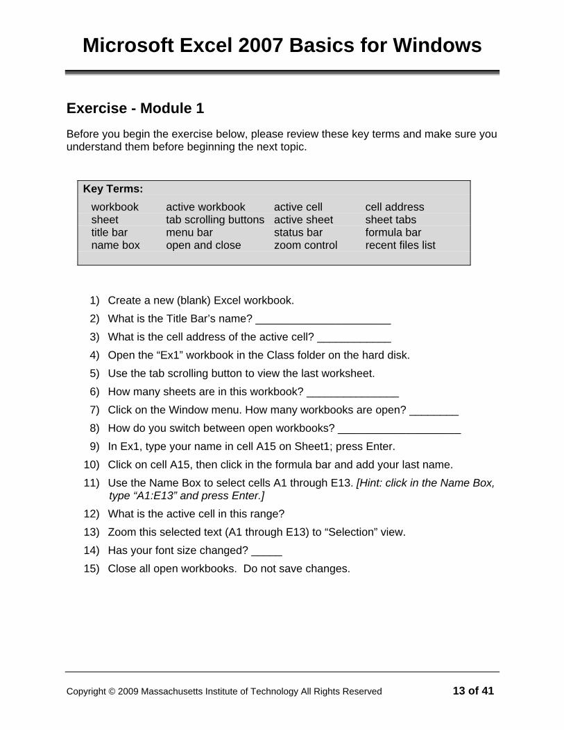
Exercise - Module 1 Before you begin the exercise below, please review these key terms and make sure you understand them before beginning the next topic.

Key Terms: workbook active workbook active cell cell address sheet tab scrolling buttons active sheet sheet tabs title bar menu bar status bar formula bar name box open and close zoom control recent files list

1) Create a new (blank) Excel workbook. 2) What is the Title Bar’s name? ______________________ 3) What is the cell address of the active cell? ____________ 4) Open the “Ex1” workbook in the Class folder on the hard disk. 5) Use the tab scrolling button to view the last worksheet. 6) How many sheets are in this workbook? _______________ 7) Click on the Window menu. How many workbooks are open? ________ 8) How do you switch between open workbooks? ____________________ 9) In Ex1, type your name in cell A15 on Sheet1; press Enter.

10) Click on cell A15, then click in the formula bar and add your last name. 11) Use the Name Box to select cells A1 through E13. [Hint: click in the Name Box,

type “A1:E13” and press Enter.] 12) What is the active cell in this range? 13) Zoom this selected text (A1 through E13) to “Selection” view. 14) Has your font size changed? _____ 15) Close all open workbooks. Do not save changes.


Module 2 – Saving

Naming workbooks To make it easier to find your workbooks, you can give them long, descriptive filenames. The complete path to the file, including drive letter, server name, folder path, and filename, can contain up to 218 characters. Filenames cannot include any of the following characters: forward slash (/), backslash (\), greater-than sign (>), less-than sign (<), asterisk (*), question mark (?), quotation mark ("), pipe symbol (|), colon (:), or semicolon (;).

Saving an unnamed workbook 1) Start a new workbook; from the Office button, click Save or Save As. 2) In the File Name box, type a name for the workbook (e.g., 1998 Budget). 3) Click the Save button.

Saving an existing workbook • On the Office button, click Save, or • Click the Save tool on the Quick Access toolbar.

Saving a copy of a workbook

1) On the Office Button, click Save As. 2) In the sub menu to the right, choose Excel Workbook 3) In the File Name box, type a new name for the workbook. 4) Click the Save button.

Note that the other workbook is automatically closed.

File name box




Saving a workbook to a new location 1) On the Office button, click Save As. 2) In the sub menu to the right, choose Excel Workbook 3) Navigate to the folder in which you wish to save a copy (e.g., Class folder). 4) Double-click on the folder, then click the Save button.

Saving a workbook with a new name and to a new location 1) On the Office button, click Save As. 2) In the sub menu to the right, choose Excel Workbook 3) In the File Name box, type a new name for the workbook. 4) Navigate to the folder in which you wish to save a copy. 5) Double-click on the folder, then click the Save button.

Note: When saving, ALL sheets in a workbook are saved.




Key Terms: save save as new name new location

1) Open the ”EX2” workbook. 2) Save the workbook as “New Name.” 3) Is “EX2” still open? ______ 4) Where is it? ____________________________________

5) Save the New Name workbook in the “Practice” folder. 6) Re-open the “EX2” workbook from the Recent Files List. 7) Close all windows. 8) Is Excel still running? _____ 9) How many workbooks are listed in the Recent Files List? _____

10) Re-open the “EX2” workbook, type your full name in B2, and save the workbook again either by using the toolbar or a keyboard shortcut.


Module 3 – Entering and Editing

Entering Worksheet Data

Enter numbers, text, a date, or a time The standard number and text settings for Excel are for entered text to be left-aligned and numbers right-aligned. Dates and times must be given specific formatting; otherwise you may get unexpected results. Time settings are right-aligned. Standard date settings are more varied. For example, if you type “1/2/97” in a cell, you will see it as “1/2/1997”. However, if you typed “January 2, 1997” in a cell, you would see “2-Jan-97” instead. If you typed “97/1/2” for the date, it would be left-aligned and you’d see what you had typed. Again, these changes are due to Excel’s standard settings. These settings can be modified, and different formatting can be applied.

Ready and Edit modes A common occurrence for new Excel users is to forget to press Enter after they enter data or make changes to the contents of a cell. When data or changes have not been entered, you cannot access some commands from the menus. When in the editing mode, the Status Bar will read “Edit.” After you press Enter, the Status Bar will read “Ready.”

When in the Edit mode, your formula bar will show a black X that turns red as you hover over it, a black check mark that turns blue as you hover over it, and an fx symbol. Clicking on the X will cancel your edit(“Esc” key works too)--]\-, clicking on the check mark will enter your edit, and clicking on the fx give you the Function Wizard dialog box which will assist you with creating a formula. The figure above shows how the formula bar looks when data has been placed in the cell but has not been entered. Figures on page 9 and 10 shows the formula bar when Excel is in the Ready mode.



Enter and edit the same data on multiple worksheets Whenever you have data that is to be repeated on several sheets, you can group the sheets first and then type your data only once. To group adjacent sheets, click on the first sheet to be grouped (can be an assumed click if already there), then Shift+Click on the last sheet to be grouped. To select nonadjacent sheets, hold down the Ctrl key while you click on the sheets you would like to group. The figure below shows these two types of grouping. Sheet1 is the active sheet because it is highlighted and bold. Sheets 1-2, and 4 are in the grouping.

Enter the same data into several cells at once If you are entering the same data into several cells, then you can use Excel’s AutoFill feature. By typing the data into the cell, then pressing and dragging its fill handle, you can repeat the data. These two figures illustrate how dragging the fill handle of “1000” to Column E would result in 1000 being repeated in the included cells.

Automatically fill in data based on adjacent cells By dragging the fill handle of a cell, you can copy the contents of that cell to other cells in the same row or column. The fill handle is a small box located at the bottom right corner of each cell. If the cell contains a number, date or time period that Excel can extend in a series, the values are incremented instead of copied. For example, if a cell contains "January," you can quickly fill in other cells in a row or column with February, March, and so on.

Fill Handle




Create a Custom List In the example above, dragging the fill handle created a list of months. You can create your own custom lists. Here’s how.

1) Select the Office button, the click Excel Options. 2) From the “Popular” index, choose, ”Edit Custom Lists…” 3) Type the entries in the List entries box, beginning with the first entry. 4) Press Enter after each entry. 5) When the list is complete, click Add (or OK).

Import an existing Custom List If you've already entered the list of items you want to use as a series, select the list on the worksheet.

1) Select the Office button, the click Excel Options. 2) From the “Popular” index, choose, ”Edit Custom Lists…” 3) To use the selected list, click Import.

Editing a custom list 1) Select the Office button, the click Excel Options. 2) From the “Popular” index, choose, ”Edit Custom Lists…” 3) Choose the list in the “List entries box, add or delete text where needed. 4) Click the Add button to accept all changes.

Editing Worksheet Data

Edit cell contents 1) Double-click the cell that contains the data you want to edit. 2) Make changes to the cell contents. 3) To enter your changes, press Enter.

Note: You can also edit in the formula bar.


Cancel , undo or redo an entry • To cancel an entry before you press Enter, press Esc. • To undo a completed entry, click Undo button on the Quick Access toolbar. • To redo the previous entry, click the Redo button on the Quick Access toolbar.

Clear contents, formats, or comments from cells 1) Select the cells, rows, or columns you want to clear.

2) From the Home tab, in the Editing button grouping, click the clear button , then click either All, Formats, Contents or Comments.





Key Terms: data fill handle custom fill cancel box check box undo redo esc clear all clear format clear comments clear contents edit in cell Edit mode Ready mode edit in formula bar

1) Open the “EX3” workbook. 2) Click on C8, then drag the fill handle to Column F. 3) What did this do? _________________________________________ 4) Create the following Custom List: Name, Address, Phone, Date of Birth 5) Open a new workbook. 6) Enter “Name” in cell B5, then press and drag B5 fill handle to Column E. 7) What happened? _________________________________________ 8) Type your first name in cell A15 and press Enter. 9) Type your last name in cell A15, then click the cancel box in the Formula Bar.

What happened? _________________________________________ 10) Choose Undo from the Edit menu. 11) Choose Redo from the Edit menu. 12) Click in cell A15 and type your middle name, then press Esc. 13) Choose Open from the Office button, then press Esc. 14) Is the Esc key more like choosing the Undo command from the Edit menu, or

like clicking on the cancel box in the Formula Bar? Explain your answer. _____________________________________________________

15) What is the difference between the cancel box [X] and the Undo command? ____________________________________________________



Module 4 – Selecting and Navigating

Selecting • To select all sheets, right-click on one of the sheet tabs, then choose Select All

Sheets from the shortcut menu.

• To select the entire row containing the selected cell, press Shift + Spacebar.

• To select the entire column containing the selected cells, press Control + Spacebar.

• To select nonadjacent sheets, Control key while you click the tabs for the sheets you want to select.

• To extend the selection from the active cell to another cell on the sheet, hold down the Shift key while clicking that cell.

• To more easily select a large range, select one corner of the range, scroll to the other corner, then depress the Shift key while you click the other corner.

• To select the entire sheet, press Control+A.

• To repeat the previous action once, press F4.

Grouping Worksheets By grouping sheets, you save time by entering repetitive data only once. Here are some techniques for grouping and ungrouping sheets.

• To group adjacent sheets, click on the first sheet to be grouped, then shift-click on the last.

• To group non-adjacent sheets, use the Control key to click on the sheets you want grouped.

• To ungroup sheets,

• If One or more sheets are not selected: click the sheet tab of the active sheet in the group, then hold down the Shift key while you click the tab of the active sheet again.

• If All Sheets are selected: click on any other sheet tab.

• Another way to ungroup sheets is to right-click on the active sheet, then from the shortcut menu, left-click on Ungroup Sheets.



Navigating • When you choose the Go To command from the Find and Select tool on the

Home tab’s Editing group, Excel adds a reference to your current location in the dialog box so you can go back easily.

• To move to the beginning of the sheet, press Control+Home.

• To move to the top of a block of data, double-click the top border of the selected cell. You can double-click the other borders to move in other directions.

• To move between cells of a worksheet, click any cell. Clicking a cell makes it the active cell.

• To bring a different area of the sheet into view, use the scroll bars.

Using the scroll bars To scroll Do this One row up or down Click arrows in vertical scroll bar. One column left or right Click arrows in horizontal scroll bar. One window up or down Click above or below scroll box in vertical scroll bar. One window left or right Click to left or right of scroll box in horizontal scroll bar. A large distance Drag scroll box in either scroll bar.

Using the keyboard To scroll Do this One cell to the right Press Tab One cell to the left Press Shift+Tab One cell down Press Enter One cell up Shift + Enter Move down one screen Page Down Move up one screen Page Up Move right one screen Alt + Page Down Move left one screen Alt + Page Up Move to next sheet Control + Page Down Move to previous sheet Control + Page Up To previous workbook Control + Tab To next workbook Shift-Control + Tab To next instance of text Control + arrow key in desired direction




Key Terms: select navigate scroll screen window left window right group ungroup

1) Open the “EX4” workbook. 2) Group Q1 Data and Q2 Data. 3) Ungroup Q1 Data and Q2 Data. 4) Use the click, shift-click method to select cells A1 through F13 on Q1 Data. 5) What is another quick method for selecting a range of cells? ___________ 6) Use a shortcut for selecting Row 5. 7) Which shortcut did you use? ________________________ 8) Use a shortcut for selecting Column A. 9) Which shortcut did you use? ________________________

10) Group Q1 Data and Q4 Data. 11) Group all four quarters. 12) Ungroup all sheets. 13) Move one screen to the right. Which shortcut did you use? ________ 14) Move to the next worksheet. Which shortcut did you use? ________ 15) Which shortcut key(s) do you think would be worth remembering? ________



Module 5 - Creating Formulas

How formulas work A formula can help you calculate data on a worksheet. You can perform operations, such as addition, multiplication, and comparison on worksheet values. You would use a formula when you want to enter calculated values on a worksheet.

A formula can include any of the following elements: operators, cell references, values, worksheet functions, and names. To enter a formula in a worksheet cell, type a combination of these elements in the formula bar. All formulas must begin with an equal sign (=).

How operators work Operators specify the operation, such as addition, subtraction, or multiplication that you want to perform on the elements of a formula.

• Arithmetic operators perform basic mathematical operations, combine numeric values, and produce numeric results.

• Comparison operators compare two values and produce the logical value TRUE or FALSE.

• A text operator joins one or more text values into a single combined text value.

In this class you will work with the addition, subtraction, multiplication and division arithmetic operators. Comparison operators and text operators will not be covered.

Creating a simple formula All formulas begin with an equal sign. Here are some examples of simple formulas: Addition + =a1+a2+a3+a4+a5 Subtraction - =a1-a27 Multiplication * =a1*d1 Division / =a1/a10

When entering formulas you can use the calculator keypad; except for equal sign, it has all the math operators for building formulas.


Using functions

The built-in functions in Microsoft Excel perform standard worksheet and macro sheet calculations. The values on which a function performs operations are called arguments.

Formula bar

• Syntax is the sequence of characters used in a formula.

• The function is “SUM.”

• The argument is “(B2:B7)” in the formula bar.

The values that the functions return are called results. You use functions by entering them into formulas on your worksheet. The sequence of characters used in a function is called the syntax. The syntax of a formula begins with an equal sign (=) and is followed by a combination of values and operators. If a function appears at the beginning of a formula, precede it with an equal sign, as with any formula.

Parentheses tell Microsoft Excel where arguments begin and end. You must include both parentheses, with no spaces before or after them. Arguments can be numbers, text, logical values, arrays, error values, or references. The argument you designate must produce a valid value for that argument. Arguments can also be constants or formulas, and the formulas can contain other functions. When an argument to a function is itself a function, it is said to be nested. In Microsoft Excel, you can nest up to seven levels of functions in a formula.

A formula does not always include a function or an argument. Consider these formulas:

=A20+B25+C50 =D19-D18 =(D6*8)+(E1/20)



Automatically sum a range of cells 1) Select the cell where you want the results to appear. 2) Click the AutoSum tool on the Home Tab in the Editing tool grouping. 3) Press the Enter key (or click the AutoSum tool again).

Sum multiple rows and columns 1) Select the rows and columns you want to sum. Make sure to add empty cells to

contain the calculation results. 2) Click the AutoSum tool.

Naming a cell or a range, or cells

Normally, once you define a name on any sheet in a workbook, you can use that name on any other sheet in the workbook. You can also create sheet-level names that can be useful if you want to use a common name on several sheets in the same workbook. If you use the same name to define both a sheet-level name and a book-level name, the sheet-level name takes precedence on the sheet where it is defined.

To name a cell or a range: 1) Select the cell, cell range, or nonadjacent selections you want to name. 2) Click the Name Box at the left end of the formula bar to activate it. 3) Type the name for the cell or range, then press Enter.


Name box as it appears after entering the name for the cell or range.

Name box as it appears after clicking in cell A1. Note: Cell reference (A1) moves to far left when you click in the Name box.


When you click the arrow next to the name box to view the list of names, you see the new cell or range name. If you select the name, Excel selects the cell or range.


There are two names in figure to right.

The is an example of using a name in a formula. Note that the formula is “=SUM(Expenses)” instead of “=SUM(B2:B7).”

An example of a “natural language” formula.

Absolute versus relative values Excel’s default setting for formulas uses relative references. In other words, when a formula is copied to another cell, the cell references are automatically adjusted relative to their last position. Absolute references are more effective for formulas which repeatedly use the same value – as in the 28% withholding rate example below. Absolute references are represented by dollar signs before column and/or row references. In the example below, E3 has been changed to $E$3. You can either type the dollar signs or press F4.

This example shows a formula for computing taxes for each employee. Rather than typing 28% in each formula, one cell has been used to place this value. It is more



fficient to refer to onee cell than typing 28% each time.

$3*F7. In other words, E3 would remain “absolute,” while F6 would be changed to F7.

Another advantage besides not having to do as much typing is that, should the withholding percentage ever change, you would not have to rewrite the formulas in every cell. For example, if the formula in G6 was copied and pasted to G7, the formula in G7 would be =$E




Key Terms: formula function syntax equal sign argument operator value (result) sum function Name Box AutoSum range of cells absolute value

1) Open the “EX5” workbook. 2) Click on the “New Hampshire” worksheet. 3) Select cells D6 through D13, then click the AutoSum tool once. 4) What happened? ____________________________________________ 5) Click in cell F6 and build a formula for the gross pay for each person. 6) Use the F6 fill handle to copy the formula down through D13. 7) What happened? ____________________________________________ 8) Click in cell G6 and create a formula for the taxes for each person.

[Hint: When creating your formula, use the cell address that has the 28% withholding tax rate.]

9) Use the G6 fill handle to copy the formula down through G13. 10) Did you get what you expected? _________ 11) If not, how would you solve this problem? 12) Click in cell H6 and build a formula for the net pay for each person. 13) Use the H6 fill handle to copy the formula down through H13. 14) Save and close your worksheet. 15) What feature will you probably use most often at work? _________



Module 6 – Formatting

Basic Worksheet Formatting • Row height and column width • Font, size, and style • Number formatting • Alignment • Borders, colors, and patterns

Applying Borders and Shading 1) Select the cells. 2) To apply the most recently selected border style, click the borders tool on the

Home tab in the Font tool group. 3) To apply a different border style, click the arrow next to borders tool, and then

click a border on the palette.

Number Formatting 1) Select the cells you want to format. 2) Click either accounting, percentage or commas, increase indent or decrease

indent button on the Number tool group on the Home tab. To select another number, date, or time format, click Cells the Number format drop down list, and then click the format you need.

Note: The number format you apply does not affect the actual cell value that Excel uses to perform calculations. The value of the active cell is displayed in the formula bar.

Style galleries replace AutoFormat Style galleries for tables, cells, and PivotTables provide a set of professional formats that can be applied quickly. You can choose from many predefined styles or create custom styles as needed. Styles replace AutoFormat as the simplest way to apply formatting to a range of cells. You can also still use the AutoFormat command, but you need to add the command to the Quick Access Toolbar first.

• Lets add this tool to the Quick Access Toolbar now


Using Styles To apply several formats in one step and ensure that cells have consistent formatting, you can apply a style to the cells. Excel provides styles to format numbers as currency, percentages, or with commas separating thousands. You can create your own styles to apply a font and font size, number formats, and cell borders and shading and to protect cells from changes.

Format Painter If you've already formatted some cells on a worksheet the way you want, you can copy the formatting to other cells using the Format Painter tool in the Clipboard tool grouping, on the Home tab.

To apply the formatting to adjacent cells:

1) Click in the cell that has the formatting you wish to duplicate. 2) Click on the Format Painter tool on the Home tab. 3) Click and drag the cell(s) that you wish to have the desired format.

To apply the formatting to non-adjacent cells:

1) Click in the cell that has the formatting you wish to copy. 2) Double-click on the Format Painter. 3) Select the cell(s) you wish to have formatted. 4) When you have finished formatting, click the Format Painter tool again, or Esc.




Exercise – Module 6 Before you begin the exercise below, please review these key terms and make sure you understand them before beginning the next topic.

Key Terms: row height column width font style font size alignment cell borders cell shading patterns autoformat format painter

1) Open the “EX6” workbook. 2) Verify that Q1 Data sheet is the active sheet. 3) Format cells A5, A8, A9, A12 and A13 as Arial, 16 Pt., Bold and Italic. 4) Click on cell A5, then double-click on the Format Painter tool. 5) Click on Q2 Data sheet, then click on cells A5, A8, A9, A12 and A13. 6) Click on the Format Painter tool. 7) Click on Q1 Data sheet. 8) Select cells A5 through F13. 9) Choose AutoFormat from the Quick Access Toolbar.

10) Select the “Colorful 1” Table Format. 11) Click on Q2 Data sheet and click in cell A5. 12) Execute the keyboard shortcut “Ctrl +Y” to repeat AutoFormat. 13) What happened? ________________________________


Module 7 - Printing

Before you print 1) Save your workbook. 2) Select Print Preview from the File menu. 3) To make changes, choose Setup.

Modify the layout of the printed worksheet You can control the appearance, or layout, of printed worksheets by changing options in the Page Setup dialog box. A worksheet can be printed in portrait or landscape orientation, and you can use different sizes of paper. Worksheet data can be centered between the left and right margins and the top and bottom margins. You can change the order of the printed pages, as well as the starting page number.

Change the worksheet area that appears on a printed page If your work doesn't fit exactly on the number of printed pages you want, you can adjust, or scale, your printed work to fit on more or fewer pages than it would at normal size. You can also specify that you want to print your work on a certain number of pages.

Print Preview To see how the page orientation, margins, headers, footers and page breaks will affect the printed worksheet before the document is printed, click the Print Preview button on the QuickAccess toolbar. To make adjustments in Print Preview, click Setup, then click on the appropriate tab and make your changes.

Print the active sheets, a selected range, or an entire workbook If the worksheet has a defined print area, Microsoft Excel will print only the print area. If you select a range of cells to print and then click Selection, Microsoft Excel prints the selection and ignores any print area defined for the worksheet.

1) From the Office Button menu, choose Print. The Print dialog box appears. 2) In the “Print What” section, select either Selection, Selected Sheet(s), or Entire

Workbook.

Tip: A faster way is to click the Quick Print tool on the Quick Access toolbar.



Create custom headers and footers You can have only one custom header and footer on each worksheet. If you create a new custom header or footer, it will replace any existing custom header or footer on the worksheet.

1) Preview your worksheet, click on the Setup button and then click on the Header/Footer tab.

2) To base a custom header or footer on an existing built-in header or footer, click the header or footer in the Header box or Footer box.

Existing built-in headers

3) To create your own, click Custom Header or Custom Footer. 4) Click in the Left section, Center section, or Right section box, and then click the

buttons to insert the header or footer information, such as the page number, that you want in that section.

This is a partial view of the Header/Footer dialog box.

5) To enter additional text for the header or footer, enter the text in the Left section, Center section, or Right section box.

6) To start a new line in one of the section boxes, press Enter. 7) To delete a section of a header or footer, select the text or symbol(s) that you

want to delete in the section box, and then press delete.



Change the font in header and footer text If you prefer to have the font type and size in your header and/or footer different from the main part of your worksheet, follow these steps to make your changes.

1) Choose Page Setup from the File menu, then click on the Header/Footer tab. 2) Click Custom Header or Custom Footer button. 3) Select the text in the Left, Center or Right section boxes.

4) Click on the button above the three sections, then make your changes. 5) Click OK when finished.

Note: You cannot change the color of header and footer text.

Print titles You can set print titles to repeat certain rows at the top of each page or repeat columns at left of each page either by choosing Page Setup from the File menu or clicking on Setup button in Print Preview dialog box.

Rows to Repeat at Top of Each Worksheet Page 1) Choose Page Setup from the File menu or click on Setup button in Print Preview

dialog box. 2) Click on the Sheet tab, then click to the right of the “Rows to Repeat at Top:”

section. 3) Click on the row(s) to repeat on your worksheet, then click OK.

Columns to Repeat at Left of Each Worksheet Page 1) Choose Page Setup from the File menu or click on Setup button in Print Preview

dialog box. 2) Click on the Sheet tab, then click to the right of the “Columns to Repeat at Left:”

section. 3) Click on the column(s) to repeat on your worksheet, then click OK.

Page Break If a worksheet is larger than one page, Microsoft Excel divides it into pages for printing by inserting automatic page breaks based on the paper size, margin settings, and




scaling options you set with the Page Setup command on the File menu. You can create manual page breaks by selecting Page Break from the Insert Menu.



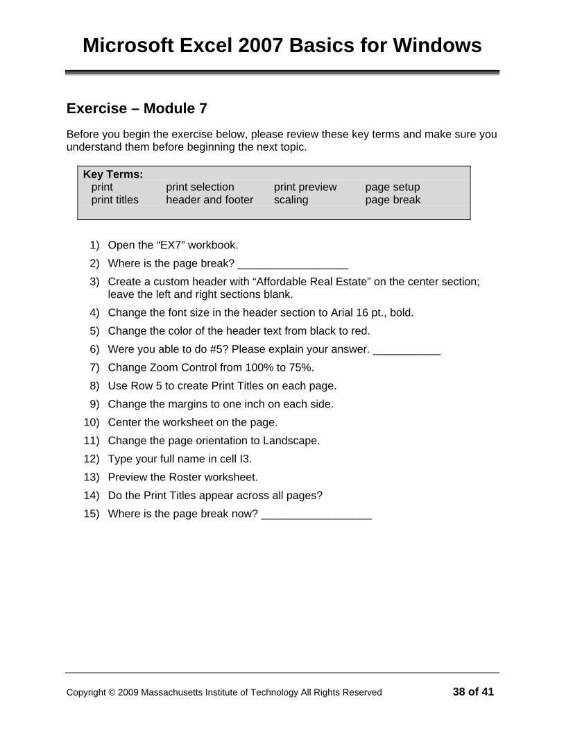
Exercise – Module 7 Before you begin the exercise below, please review these key terms and make sure you understand them before beginning the next topic.

Key Terms: print print selection print preview page setup print titles header and footer scaling page break

1) Open the “EX7” workbook. 2) Where is the page break? __________________ 3) Create a custom header with “Affordable Real Estate” on the center section;

leave the left and right sections blank. 4) Change the font size in the header section to Arial 16 pt., bold. 5) Change the color of the header text from black to red. 6) Were you able to do #5? Please explain your answer. ___________ 7) Change Zoom Control from 100% to 75%. 8) Use Row 5 to create Print Titles on each page. 9) Change the margins to one inch on each side.

10) Center the worksheet on the page. 11) Change the page orientation to Landscape. 12) Type your full name in cell I3. 13) Preview the Roster worksheet. 14) Do the Print Titles appear across all pages? 15) Where is the page break now? __________________


Module 8 – Getting Help

When you have a question First look in Microsoft’s online Help.

Office Assistant tool The Office Help tool (the one on the Ribbon that has a question mark in it) provides tips about more efficient ways to do your work. Clicking on the button will display the Help dialog box.

Dialog Box Screen Tips You can find out what each dialog box item does without interrupting your work. To see a dialog box ScreenTip:

1) While viewing a dialog box, left-click on the question mark button in the dialog box’s title bar. Your mouse pointer change to a pointer with a black question mark next to it.

2) Click on the item in the dialog box that you’d like to know about. A small window with a brief description of the item will appear.

3) If the dialog box doesn’t have a question mark button, look for a Help button or press the F1 key.

The dialog box Screen Tip button is on the right side of the title bar.

Toolbar Screen Tips To see the name of a ribbon button, position the pointer (but don’t click) over the button; a small label with the name of the tool will appear below the ribbon.

MIT Computing Help Desk The Computing Help Desk can answer your questions and assist with problems related to Microsoft Excel and other software applications.



They can be reached three ways:

• Phone at (617) 253-1101 on weekdays between 8 am and 6pm.

• Send e-mail to [email protected].

• Access through the Web at http://ist.mit.edu/support.

MIT Excel User Group The Excel User Group meets on the first Tuesday of each month; September – June, to share information. It is one of many user groups that meet on campus. To see a complete list of user groups at MIT, go to:

• http://ist.mit.edu/support/usergroups



Key Terms: Getting Results Screen Tips User Group Help Desk World Wide Web

For more information, contact John Fothergill, the Excel User Group coordinator, at (617) 253-5312 or send email to the Excel User Group list [email protected]. The Excel User Group web page is at http://web.mit.edu/xlug/.



1) Open the “EX8” workbook.

2) Use Screen Tips to learn what the tool with the triangle, square and circle does. What is the name of this tool? ______________________________

3) What is the web address for the Excel User Group? __________________

4) What is the email address for the Excel User Group? _________________

5) Write the Help Disk phone number for Excel for Windows here. _________

6) Click on the context sensitive help button, then choose Subtotals from the Data menu.

7) Close all open windows and Exit the Excel program.

CONGRATULATIONS! YOU HAVE SUCCESSFULLY COMPLETED THIS COURSE.