microsoft research - github pagesmicrosoft research oregon 2008 – p.1/168 overview satisﬁability...

SMT Solvers: Theory and Implementation

Summer School on Logic and Theorem Proving

Leonardo de Moura

[email protected]

Microsoft Research

Oregon 2008 – p.1/168

Overview

Satisfiability is the problem of determining if a formula has a model.

In the purely Boolean case, a model is a truth assignment to the

Boolean variables.

In the first-order case, a model assigns values from a domain to

variables and interpretations over the domain to the function and

predicate symbols.

For theories such arithmetic, a model admits a specific (range of)

interpretation to the arithmetic symbols.

Efficient SAT and SMT solvers have many applications.

Oregon 2008 – p.2/168

Applications

Extended Static Checking.

Spec#, VCC, HAVOC

ESC/Java

Predicate Abstraction.

SLAM/SDV (device driver verification).

Test-case generation.

Pex, Sage

Bounded Model Checking (BMC) & k-induction.

Symbolic Simulation.

Planning & Scheduling.

Equivalence checking.

Oregon 2008 – p.3/168

SMT-Solvers & SMT-Lib & SMT-Comp

SMT-Solvers:

Alt-Ergo, Ario, Barcelogic, Beaver, Boolector, CVC, CVC

Lite, CVC3, DPT (Intel), ExtSAT, Harvey, HTP, ICS (SRI),

Jat, MathSAT, OpenSMT, Sateen, Simplify, Spear, STeP,

STP, SVC, Sword, TSAT, UCLID, Yices (SRI), Zap, Zapato,

Z3 (Microsoft)

SMT-Lib: library of benchmarks

http://www.smtlib.org

SMT-Comp: annual SMT-Solver competition

http://www.smtcomp.org

Oregon 2008 – p.4/168



Goals

This tutorial covers pragmatic issues in the theory, implementation,

and use of SMT solvers.

It is not a comprehensive survey, but a basic and rigorous

introduction to some of the key ideas.

It is not directed at experts but at potential users and developers of

SMT solvers.

Oregon 2008 – p.5/168

Roadmap

Background

SAT & SMT

Equality

Arithmetic

Combining theories

Quantifiers

Applications

Oregon 2008 – p.6/168

Logic Basics

Logic studies the trinity between language, interpretation and proof.

Language circumscribes the syntax that is used to construct

sensible assertions.

Interpretation ascribes an intended sense to these assertions by

fixing the meaning of certain symbols, e.g., the logical connectives,

and delimiting the variation in the meanings of other symbols, e.g.,

variables, functions, and predicates.

An assertion is valid if it holds in all interpretations.

Checking validity through interpretations is typically not feasible, so

proofs in the form axioms and inference rules are used to

demonstrate the validity of assertions.

Oregon 2008 – p.7/168

Language: Signatures

A signature Σ is a finite set of:

Function symbols: ΣF = {f, g, . . .}.

Predicate symbols: ΣP = {p, q, . . .}.

and an arity function: Σ 7→ N

Function symbols with arity 0 are called constants.

A countable set V of variables disjoint of Σ.

Oregon 2008 – p.8/168

Language: Terms

The set T (Σ,V) of terms is the smallest set such that:

V ⊂ T (Σ,V)

f(t1, . . . , tn) ∈ T (Σ,V) whenever

f ∈ ΣF , t1, . . . , tn ∈ T (Σ,V) and arity(f) = n.

The set of ground terms is defined as T (Σ, ∅).

Oregon 2008 – p.9/168

Language: Atomic Formulas

p(t1, . . . , tn) is an atomic formula whenever

p ∈ ΣP , arity(p) = n, and t1, . . . , tn ∈ T (Σ,V).

true and false are atomic formulas.

If t1, . . . , tn are ground terms, then p(t1, . . . , tn) is called a

ground (atomic) formula.

We assume that the binary predicate = is present in ΣP .

A literal is an atomic formula or its negation.

Oregon 2008 – p.10/168

Language: Quantifier Free Formulas

The set QFF(Σ,V) of quantifier free formulas is the smallest set

such that:

Every atomic formulas is in QFF(Σ,V).

If φ ∈ QFF(Σ,V), then ¬φ ∈ QFF(Σ,V).

If φ1, φ2 ∈ QFF(Σ,V), then

φ1 ∧ φ2 ∈ QFF(Σ,V)

φ1 ∨ φ2 ∈ QFF(Σ,V)

φ1 ⇒ φ2 ∈ QFF(Σ,V)

φ1 ⇔ φ2 ∈ QFF(Σ,V)

Oregon 2008 – p.11/168

Language: Formulas

The set of first-order formulas is the closure of QFF(Σ,V) under

existential (∃) and universal (∀) quantification.

Free (occurrences) of variables in a formula are those not bound by

a quantifier.

A sentence is a first-order formula with no free variables.

Oregon 2008 – p.12/168

Models (Semantics)

A model M is defined as:

Domain |M |: set of elements.

Interpretation M(f) : |M |n 7→ |M | for each f ∈ ΣF with

arity(f) = n.

Interpretation M(p) ⊆ |M |n for each p ∈ ΣP with

arity(p) = n.

Assignment M(x) ∈ |M | for every variable x ∈ V .

A formula φ is true in a model M if it evaluates to true under the

given interpretations over the domain |M |.

Oregon 2008 – p.13/168

Interpreting Terms

M [[x]] = M(x)

M [[f(a1, . . . , an)]] = M(f)(M [[a1]], . . . ,M [[an]])

Oregon 2008 – p.14/168

Interpreting Formulas

The interpretation of a formula F in M , M [[F ]], is defined as

M |= a = b ⇐⇒ M [[a]] = M [[b]]

M |= p(a1, . . . , an) ⇐⇒ 〈M [[a1]], . . . ,M [[an]]〉 ∈M(p)

M |= ¬ψ ⇐⇒ M 6|= ψ

M |= ψ1 ∨ ψ2 ⇐⇒ M |= ψ1 or M |= ψ2

M |= ψ1 ∧ ψ2 ⇐⇒ M |= ψ1 and M |= ψ2

M |= (∀x : ψ) ⇐⇒ M{x 7→ a} |= ψ, for all a ∈ |M |

M |= (∃x : ψ) ⇐⇒ M{x 7→ a} |= ψ, for some a ∈ |M |

Oregon 2008 – p.15/168

Interpretation Example

Σ = {0,+, <}, and M such that |M | = {a, b, c}

M(0) = a,

M(+) = {〈a, a 7→ a〉, 〈a, b 7→ b〉, 〈a, c 7→ c〉, 〈b, a 7→ b〉, 〈b, b 7→ c〉,

〈b, c 7→ a〉, 〈c, a 7→ c〉, 〈c, b 7→ a〉, 〈c, c 7→ b〉}

M(<) = {〈a, b〉, 〈a, c〉, 〈b, c〉}

If M(x) = a,M(y) = b,M(z) = c, then

M [[+(+(x, y), z)]] =

M(+)(M(+)(M(x),M(y)),M(z)) = M(+)(M(+)(a, b), c) =

M(+)(b, c) = a

Oregon 2008 – p.16/168

Interpretation Example

Σ = {0,+, <}, and M such that |M | = {a, b, c}

M(0) = a,

M(+) = {〈a, a 7→ a〉, 〈a, b 7→ b〉, 〈a, c 7→ c〉, 〈b, a 7→ b〉, 〈b, b 7→ c〉,

〈b, c 7→ a〉, 〈c, a 7→ c〉, 〈c, b 7→ a〉, 〈c, c 7→ b〉}

M(<) = {〈a, b〉, 〈a, c〉, 〈b, c〉}

M |= (∀x : (∃y : +(x, y) = 0))

M 6|= (∀x : (∃y : x < y))

M |= (∀x : (∃y : +(x, y) = x))

Oregon 2008 – p.17/168

Validity

A formula F is satisfiable if there is an interpretation M such that

M |= F .

Otherwise, the formula F is unsatisfiable.

If a formula is satisfiable, so is its existential closure ∃~x : F , where

~x is vars(F ), the set of free variables in F .

If a formula F is unsatisfiable, then the negation of its existential

closure ¬∃~x : F is valid.

Oregon 2008 – p.18/168

Theories

A (first-order) theory T (over a signature Σ) is a set of (deductively

closed) sentences (over Σ and V ).

Let DC(Γ) be the deductive closure of a set of sentences Γ.

For every theory T , DC(T ) = T .

A theory T is consistent if false 6∈ T .

We can view a (first-order) theory T as the class of all models of

T (due to completeness of first-order logic).

Oregon 2008 – p.19/168

Satisfiability and Validity

A formula φ(~x) is satisfiable in a theory T if there is a model of

DC(T ∪ ∃~x.φ(~x)). That is, there is a model M for T in which

φ(~x) evaluates to true, denoted by,

M |=T φ(~x)

This is also called T -satisfiability.

A formula φ(~x) is valid in a theory T if ∀~x.φ(~x) ∈ T . That is

φ(~x) evaluates to true in every model M of T .

T -validity is denoted by |=T φ(~x).

The quantifier free T -satisfiability problem restricts φ to be

quantifier free.

Oregon 2008 – p.20/168

Roadmap

Background

SAT & SMT

Combining theories

Equality

Arithmetic

Quantifiers

Applications

Oregon 2008 – p.21/168

Clausal (CNF) Form

In clausal form, the formula is a set (conjunction) of clauses∧

iCi, and

each clause Ci is a disjunction of literals. A literal is an atom or the

negation of an atom.

p1 ∨ ¬p2, ¬p1 ∨ p2 ∨ p3, p3

Most SAT solvers assume the formula is in CNF.

Naıve translation to CNF is too expensive.

Oregon 2008 – p.22/168

Conversion to Clausal (CNF) Form

CNF (p,∆) = 〈p,∆〉

CNF (¬φ,∆) = 〈¬l,∆′〉, where 〈l,∆′〉 = CNF (φ,∆)

CNF (φ1 ∧ φ2,∆) = 〈p,∆′〉, where

〈l1,∆1〉 = CNF (φ1,∆)

〈l2,∆2〉 = CNF (φ2,∆1)

p is fresh

∆′ = ∆2 ∪ {¬p ∨ l1,¬p ∨ l2,¬l1 ∨ ¬l2 ∨ p}

CNF (φ1 ∨ φ2,∆) = 〈p,∆′〉, where . . .

∆′ = ∆2 ∪ {¬p ∨ l1 ∨ l2,¬l1 ∨ p,¬l2 ∨ p}

Theorem: φ and l∧∆ are equisatisfiable, where CNF(φ, ∅) = 〈l,∆〉.Oregon 2008 – p.23/168

Conversion to CNF: Example

CNF (¬(q1 ∧

p1︷︸︸︷

(q2 ∨ ¬q3)︸︷︷︸

p2

), ∅) =

〈¬p2, { ¬p1 ∨ q2 ∨ ¬q3,

¬q2 ∨ p1,

q3 ∨ p1,

¬p2 ∨ q1,

¬p2 ∨ p1,

¬q1 ∨ ¬p1 ∨ p2}〉

Oregon 2008 – p.24/168

Conversion to CNF

Improvements:

Maximize sharing & canonicity in the input formula F .

Cache φ 7→ l, when CNF (φ,∆) = 〈l,∆′〉.

Support for multiary ∨ and ∧.

. . .

Oregon 2008 – p.25/168

Resolution

Input: a set of clauses.

No duplicate literals in clauses.

Tautologies, clauses containing l and l, are deleted.

Rules:

F, C ∨ l, D ∨ l =⇒ F, C ∨ l, D ∨ l, C ∨D

F, l, l =⇒ unsat

Improvement: ordered resolution.

Oregon 2008 – p.26/168

Resolution: Example

¬p ∨ ¬q ∨ r, ¬p ∨ q, p ∨ r, ¬r

Oregon 2008 – p.27/168

Resolution: Example

¬p ∨ ¬q ∨ r, ¬p ∨ q, p ∨ r, ¬r ⇒

¬p ∨ ¬q ∨ r, ¬p ∨ q, p ∨ r, ¬r, ¬q ∨ r

Oregon 2008 – p.27/168

Resolution: Example

¬p ∨ ¬q ∨ r, ¬p ∨ q, p ∨ r, ¬r ⇒

¬p ∨ ¬q ∨ r, ¬p ∨ q, p ∨ r, ¬r, ¬q ∨ r ⇒

¬p ∨ ¬q ∨ r, ¬p ∨ q, p ∨ r, ¬r, ¬q ∨ r, q ∨ r

Oregon 2008 – p.27/168

Resolution: Example

¬p ∨ ¬q ∨ r, ¬p ∨ q, p ∨ r, ¬r ⇒

¬p ∨ ¬q ∨ r, ¬p ∨ q, p ∨ r, ¬r, ¬q ∨ r ⇒

¬p ∨ ¬q ∨ r, ¬p ∨ q, p ∨ r, ¬r, ¬q ∨ r, q ∨ r ⇒

¬p ∨ ¬q ∨ r, ¬p ∨ q, p ∨ r, ¬r, ¬q ∨ r, q ∨ r, r

Oregon 2008 – p.27/168

Resolution: Example

¬p ∨ ¬q ∨ r, ¬p ∨ q, p ∨ r, ¬r ⇒

¬p ∨ ¬q ∨ r, ¬p ∨ q, p ∨ r, ¬r, ¬q ∨ r ⇒

¬p ∨ ¬q ∨ r, ¬p ∨ q, p ∨ r, ¬r, ¬q ∨ r, q ∨ r ⇒

¬p ∨ ¬q ∨ r, ¬p ∨ q, p ∨ r, ¬r, ¬q ∨ r, q ∨ r, r ⇒

unsat

Oregon 2008 – p.27/168

Resolution: Correctness

Progress: Bounded number of clauses. Each application of resolution

generates a new clause.

Conservation: For any model M , if M |= C ∨ l and M |= D ∨ l,

then M |= C ∨D.

Canonicity: Given an irreducible non-unsat state in the atoms

p1, . . . , pn with pi ≺ pi+1, build a series of partial interpretations

Mi as follows:

1. Let M0 = ∅

2. If pi+1 is not the maximal atom in some clause that is not

already satisfied in Mi, then Mi+1 = Mi[pi+1 := false].

3. If some pi+1 ∨ C is not already satisfied in Mi, then

Mi+1 = Mi[pi+1 := true].

Oregon 2008 – p.28/168

The (original) DPLL Procedure

Resolution is not practical (exponential amount of memory).

DPLL tries to build incrementally a model M for a CNF formula F .

M is grown by:

deducing the truth value of a literal from M and F , or

guessing a truth value.

If a wrong guess leads to an inconsistency, the procedure

backtracks and tries the opposite one.

Oregon 2008 – p.29/168

Breakthrough in SAT solving

Modern SAT solvers are based on the DPLL algorithm.

Modern implementations add several sophisticated search

techniques.

Backjumping

Learning

Restarts

Indexing

Oregon 2008 – p.30/168

Abstract DPLL

M ||F =⇒ M l ||F if

8

<

:

l or l occurs in F,

l is undefined in M(Decide )

M ||F, C ∨ l =⇒ M lC∨l ||F, C ∨ l if

8

<

:

M |= ¬C,

l is undefined in M(UnitPropagate )

M ||F, C =⇒ M ||F, C ||C if M |= ¬C (Conflict )

M ||F ||C ∨ l =⇒ M ||F ||D ∨ C if lD∨l ∈ M, (Resolve )

M ||F ||C =⇒ M ||F, C ||C if C 6∈ F (Learn )

M l′ M ′ ||F ||C ∨ l =⇒ M lC∨l ||F if

8

<

:

M |= ¬C,

l is undefined in M(Backjump )

M ||F ||� =⇒ unsat (Unsat )

Oregon 2008 – p.31/168

Abstract DPLL: Example

|| 1 ∨ 2, 3 ∨ 4, 5 ∨ 6, 6 ∨ 5 ∨ 2

Oregon 2008 – p.32/168


|| 1 ∨ 2, 3 ∨ 4, 5 ∨ 6, 6 ∨ 5 ∨ 2 ⇒ (Decide)

1 || 1 ∨ 2, 3 ∨ 4, 5 ∨ 6, 6 ∨ 5 ∨ 2

Oregon 2008 – p.32/168


|| 1 ∨ 2, 3 ∨ 4, 5 ∨ 6, 6 ∨ 5 ∨ 2 ⇒ (Decide)

1 || 1 ∨ 2, 3 ∨ 4, 5 ∨ 6, 6 ∨ 5 ∨ 2 ⇒ (UnitProp)

1 21∨2 || 1 ∨ 2, 3 ∨ 4, 5 ∨ 6, 6 ∨ 5 ∨ 2

Oregon 2008 – p.32/168


|| 1 ∨ 2, 3 ∨ 4, 5 ∨ 6, 6 ∨ 5 ∨ 2 ⇒ (Decide)

1 || 1 ∨ 2, 3 ∨ 4, 5 ∨ 6, 6 ∨ 5 ∨ 2 ⇒ (UnitProp)

1 21∨2 || 1 ∨ 2, 3 ∨ 4, 5 ∨ 6, 6 ∨ 5 ∨ 2 ⇒ (Decide)

1 21∨2 3 || 1 ∨ 2, 3 ∨ 4, 5 ∨ 6, 6 ∨ 5 ∨ 2

Oregon 2008 – p.32/168


|| 1 ∨ 2, 3 ∨ 4, 5 ∨ 6, 6 ∨ 5 ∨ 2 ⇒ (Decide)

1 || 1 ∨ 2, 3 ∨ 4, 5 ∨ 6, 6 ∨ 5 ∨ 2 ⇒ (UnitProp)

1 21∨2 || 1 ∨ 2, 3 ∨ 4, 5 ∨ 6, 6 ∨ 5 ∨ 2 ⇒ (Decide)

1 21∨2 3 || 1 ∨ 2, 3 ∨ 4, 5 ∨ 6, 6 ∨ 5 ∨ 2 ⇒ (UnitProp)

1 21∨2 3 43∨4 || 1 ∨ 2, 3 ∨ 4, 5 ∨ 6, 6 ∨ 5 ∨ 2

Oregon 2008 – p.32/168


|| 1 ∨ 2, 3 ∨ 4, 5 ∨ 6, 6 ∨ 5 ∨ 2 ⇒ (Decide)

1 || 1 ∨ 2, 3 ∨ 4, 5 ∨ 6, 6 ∨ 5 ∨ 2 ⇒ (UnitProp)

1 21∨2 || 1 ∨ 2, 3 ∨ 4, 5 ∨ 6, 6 ∨ 5 ∨ 2 ⇒ (Decide)

1 21∨2 3 || 1 ∨ 2, 3 ∨ 4, 5 ∨ 6, 6 ∨ 5 ∨ 2 ⇒ (UnitProp)

1 21∨2 3 43∨4 || 1 ∨ 2, 3 ∨ 4, 5 ∨ 6, 6 ∨ 5 ∨ 2 ⇒ (Decide)

1 21∨2 3 43∨4 5 || 1 ∨ 2, 3 ∨ 4, 5 ∨ 6, 6 ∨ 5 ∨ 2

Oregon 2008 – p.32/168


|| 1 ∨ 2, 3 ∨ 4, 5 ∨ 6, 6 ∨ 5 ∨ 2 ⇒ (Decide)

1 || 1 ∨ 2, 3 ∨ 4, 5 ∨ 6, 6 ∨ 5 ∨ 2 ⇒ (UnitProp)

1 21∨2 || 1 ∨ 2, 3 ∨ 4, 5 ∨ 6, 6 ∨ 5 ∨ 2 ⇒ (Decide)

1 21∨2 3 || 1 ∨ 2, 3 ∨ 4, 5 ∨ 6, 6 ∨ 5 ∨ 2 ⇒ (UnitProp)

1 21∨2 3 43∨4 || 1 ∨ 2, 3 ∨ 4, 5 ∨ 6, 6 ∨ 5 ∨ 2 ⇒ (Decide)

1 21∨2 3 43∨4 5 || 1 ∨ 2, 3 ∨ 4, 5 ∨ 6, 6 ∨ 5 ∨ 2 ⇒ (UnitProp)

1 21∨2 3 43∨4 5 65∨6 || 1 ∨ 2, 3 ∨ 4, 5 ∨ 6, 6 ∨ 5 ∨ 2

Oregon 2008 – p.32/168


|| 1 ∨ 2, 3 ∨ 4, 5 ∨ 6, 6 ∨ 5 ∨ 2 ⇒ (Decide)

1 || 1 ∨ 2, 3 ∨ 4, 5 ∨ 6, 6 ∨ 5 ∨ 2 ⇒ (UnitProp)

1 21∨2 || 1 ∨ 2, 3 ∨ 4, 5 ∨ 6, 6 ∨ 5 ∨ 2 ⇒ (Decide)

1 21∨2 3 || 1 ∨ 2, 3 ∨ 4, 5 ∨ 6, 6 ∨ 5 ∨ 2 ⇒ (UnitProp)

1 21∨2 3 43∨4 || 1 ∨ 2, 3 ∨ 4, 5 ∨ 6, 6 ∨ 5 ∨ 2 ⇒ (Decide)

1 21∨2 3 43∨4 5 || 1 ∨ 2, 3 ∨ 4, 5 ∨ 6, 6 ∨ 5 ∨ 2 ⇒ (UnitProp)

1 21∨2 3 43∨4 5 65∨6 || 1 ∨ 2, 3 ∨ 4, 5 ∨ 6, 6 ∨ 5 ∨ 2 ⇒ (Conflict)

1 21∨2 3 43∨4 5 65∨6 || 1 ∨ 2, 3 ∨ 4, 5 ∨ 6, 6 ∨ 5 ∨ 2 || 6 ∨ 5 ∨ 2

Oregon 2008 – p.32/168


|| 1 ∨ 2, 3 ∨ 4, 5 ∨ 6, 6 ∨ 5 ∨ 2 ⇒ (Decide)

1 || 1 ∨ 2, 3 ∨ 4, 5 ∨ 6, 6 ∨ 5 ∨ 2 ⇒ (UnitProp)

1 21∨2 || 1 ∨ 2, 3 ∨ 4, 5 ∨ 6, 6 ∨ 5 ∨ 2 ⇒ (Decide)

1 21∨2 3 || 1 ∨ 2, 3 ∨ 4, 5 ∨ 6, 6 ∨ 5 ∨ 2 ⇒ (UnitProp)

1 21∨2 3 43∨4 || 1 ∨ 2, 3 ∨ 4, 5 ∨ 6, 6 ∨ 5 ∨ 2 ⇒ (Decide)

1 21∨2 3 43∨4 5 || 1 ∨ 2, 3 ∨ 4, 5 ∨ 6, 6 ∨ 5 ∨ 2 ⇒ (UnitProp)

1 21∨2 3 43∨4 5 65∨6 || 1 ∨ 2, 3 ∨ 4, 5 ∨ 6, 6 ∨ 5 ∨ 2 ⇒ (Conflict)

1 21∨2 3 43∨4 5 65∨6 || 1 ∨ 2, 3 ∨ 4, 5 ∨ 6, 6 ∨ 5 ∨ 2︸︷︷︸

F

|| 6 ∨ 5 ∨ 2

Oregon 2008 – p.32/168

Abstract DPLL: Example (cont.)

1 21∨2 3 43∨4 5 65∨6 || F || 6 ∨ 5 ∨ 2

Oregon 2008 – p.33/168


1 21∨2 3 43∨4 5 65∨6 || F || 6 ∨ 5 ∨ 2 ⇒ (Resolve)

1 21∨2 3 43∨4 5 65∨6 || F || 5 ∨ 2

Oregon 2008 – p.33/168


1 21∨2 3 43∨4 5 65∨6 || F || 6 ∨ 5 ∨ 2 ⇒ (Resolve)

1 21∨2 3 43∨4 5 65∨6 || F || 5 ∨ 2 ⇒ (Learn)

1 21∨2 3 43∨4 5 65∨6 || F, 5 ∨ 2 || 5 ∨ 2

Oregon 2008 – p.33/168


1 21∨2 3 43∨4 5 65∨6 || F || 6 ∨ 5 ∨ 2 ⇒ (Resolve)

1 21∨2 3 43∨4 5 65∨6 || F || 5 ∨ 2 ⇒ (Learn)

1 21∨2 3 43∨4 5 65∨6 || F, 5 ∨ 2 || 5 ∨ 2 ⇒ (Resolve)

1 21∨2 3 43∨4 5 65∨6 || F, 5 ∨ 2 || 5 ∨ 1

Oregon 2008 – p.33/168


1 21∨2 3 43∨4 5 65∨6 || F || 6 ∨ 5 ∨ 2 ⇒ (Resolve)

1 21∨2 3 43∨4 5 65∨6 || F || 5 ∨ 2 ⇒ (Learn)

1 21∨2 3 43∨4 5 65∨6 || F, 5 ∨ 2 || 5 ∨ 2 ⇒ (Resolve)

1 21∨2 3 43∨4 5 65∨6 || F, 5 ∨ 2 || 5 ∨ 1 ⇒ (Backjump)

1 21∨2 55∨1 || F, 5 ∨ 2

Oregon 2008 – p.33/168

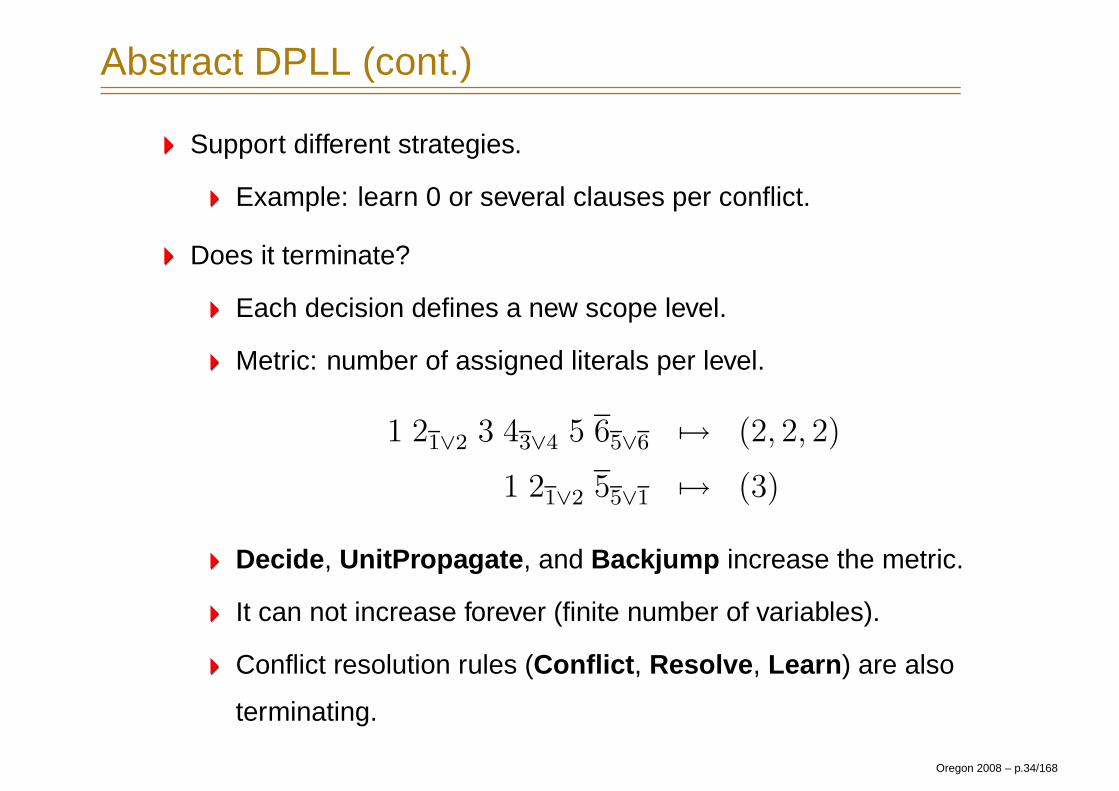
Abstract DPLL (cont.)

Support different strategies.

Example: learn 0 or several clauses per conflict.

Does it terminate?

Each decision defines a new scope level.

Metric: number of assigned literals per level.

1 21∨2 3 43∨4 5 65∨6 7→ (2, 2, 2)

1 21∨2 55∨1 7→ (3)

Decide , UnitPropagate , and Backjump increase the metric.

It can not increase forever (finite number of variables).

Conflict resolution rules (Conflict , Resolve , Learn ) are also

terminating.

Oregon 2008 – p.34/168

Abstract DPLL: Strategy

Abstract DPLL is very flexible.

Basic Strategy:

Only apply Decide if UnitPropagate and Conflict cannot be

applied.

Conflict Resolution:

Learn only one clause per conflict (the clause used in

Backjump ).

Use Backjump as soon as possible (FUIP).Use the rightmost (applicable) literal in M when applyingResolve .M ||F ||C ∨ l =⇒ M ||F ||D ∨ C if lD∨l ∈ M, (Resolve )

Oregon 2008 – p.35/168

Abstract DPLL: Decision Strategy

Decision heuristic:

Associate a score with each boolean variable.

Select the variable with highest score when Decide is used.Increase by δ the score of var(l) when Resolve is used:M ||F ||C ∨ l =⇒ M ||F ||D ∨ C if lD∨l ∈ M, (Resolve )

Increase the score of every variable in the clause C ∨ l whenBackjump is used:

M l′ M ′ ||F ||C ∨ l =⇒ M lC∨l ||F′ if

8

<

:

M |= ¬C,

l is undefined in M(Backjump )

After each conflict: slightly increase the value of δ.

From time to time renormalize the scores and δ to avoid

overflows.

Oregon 2008 – p.36/168

Abstract DPLL: Phase Selection

Assume p was selected by a decision strategy.

Should we assign p or ¬p in Decide ?

Always False Guess ¬p (works well in practice).

Always True Guess p.

Score Associate a score with each literal instead of each variable.

Pick the phase with highest score.

Caching Caches the last phase of variables during conflict

resolution. Improvement: except for variables in the last

decision level.

Greedy Select the phase that satisfies most clauses.

Oregon 2008 – p.37/168

Abstract DPLL: Extra Rules

Extra rules:

M ||F, C =⇒ M ||F if C is a learned clause (Forget )

M ||F =⇒ ||F (Restart )

Forget in practice:

Associate a score with each learned clause C .Increase by δc the score of D ∨ l when Resolve is used.M ||F ||C ∨ l =⇒ M ||F ||D ∨ C if lD∨l ∈ M, (Resolve )

From time to time use Forget to delete learned clauses with

low score.

Oregon 2008 – p.38/168

Abstract DPLL: Restart Strategies

No restarts

Linear Restart after every k conflicts, update k := k + δ.

Geometric Restart after every k conflicts, update k := k × δ.

Inner-Out Geometric “Two dimensional pattern” that increases in both

dimensions.

Initially k := x, the inner loop multiplies k by δ at each restart.

When k > y, k := x and y := y × δ.

Luby Restarts are performed according to the following series:1, 1, 2, 1, 1, 2, 4, 1, 1, 2, 1, 1, 2, 4, 8, . . ., multiplied by a constantc (e.g., 100, 256, 512).

luby(i) =

8

<

:

2k−1, if ∃k. i = 2k − 1

luby(i − 2k−1 + 1), if ∃k. 2k−1 ≤ i < 2k − 1

Oregon 2008 – p.39/168

Indexing

Indexing techniques are very important.

How to implement UnitPropagate and Conflict ?

Scanning the set of clauses will not scale.

Simple index: mapping from literals to clauses (occurrences).

watch(l) = {C1, . . . , Cn}, where l ∈ Ci

If l is assigned, check each clause C ∈ watch(l) for

UnitPropagate and Conflict .

Most of the time C has more than one unassigned literal.

Improvement: associate a counter u with each clause (number

of unassigned literals).

Problem: counters must be decremented when literals are

assigned, and restored during Backjump .

Oregon 2008 – p.40/168

Indexing: Two Watch Literal

Insight:

No need to include clause C in every set watch(l) where

l ∈ C .

It suffices to include C in at most 2 such sets.

Invariant:

If some literal l in C is not assigned to false, then

C ∈ watch(l′) of some l′ that is not assigned to false.

Oregon 2008 – p.41/168

Indexing: Two watch Literal

Maintain 2-watch invariant:

Whenever l is assigned.

For each clause C ∈ watch(l)

If the other watch literal l′ (C ∈ watch(l′)) is assigned to

true, then do nothing.

Else if some other literal l′ is true or unassigned

watch(l′) := watch(l′) ∪ {C}

watch(l) := watch(l) \ {C}

Else if all literals in C are assigned to false, then Backjump .

Else (all but one literal in C is assigned to false) Propagate .

Oregon 2008 – p.42/168

Preprocessor

Preprocessing step is very important for industrial benchmarks.

Formula CNF (already covered).

Subsumption: C subsumes D if C ⊆ D.

Resolution: eliminate cheap variables.

occs(l) = {clauses that contain l}

|occs(p)| ∗ |occs(¬p)| < k

|occs(p)| = 1 or |occs(¬p)| = 1

Oregon 2008 – p.43/168

Satisfiability Modulo Theories (SMT)

In SMT solving, the Boolean atoms represent constraints over

individual variables ranging over integer, reals, bit-vectors,

datatypes, and arrays.

The constraints can involve theory operations, equality, and

inequality.

Now, the SAT solver has to interact with theory solvers.

The constraint solver can detect conflicts involving theory

reasoning, e.g., f(x) 6= f(y), x = y, or

x− y ≤ 2, y − z ≤ −1, z − x ≤ −3.

Oregon 2008 – p.44/168

Pure Theory of Equality (EUF)

The theory T E of equality is the theory DC(∅).

The exact set of sentences of T E depends on the signature in

question.

The theory does not restrict the possibles values of the symbols in

its signature in any way. For this reason, it is sometimes called the

theory of equality and uninterpreted functions.

The satisfiability problem for T E is the satisfiability problem for

first-order logic, which is undecidable.

The satisfiability problem for conjunction of literals in T E is

decidable in polynomial time using congruence closure.

Oregon 2008 – p.45/168

Linear Integer Arithmetic

ΣP = {≤}, ΣF = {0, 1,+,−}.

Let MLIA be the standard model of integers.

Then T LIA is defined to be the set of all Σ sentences true in the

model MLIA.

As showed by Presburger, the general satisfiability problem for

T LIA is decidable, but its complexity is triply-exponential.

The quantifier free satisfiability problem is NP-complete.

Remark: non-linear integer arithmetic is undecidable even for the

quantifier free case.

Oregon 2008 – p.46/168

Linear Real Arithmetic

The general satisfiability problem for T LRA is decidable, but its

complexity is doubly-exponential.

The quantifier free satisfiability problem is solvable in polynomial

time, though exponential methods (Simplex) tend to perform best in

practice.

Oregon 2008 – p.47/168

Difference Logic

Difference logic is a fragment of linear arithmetic.

Atoms have the form: x− y ≤ c.

Most linear arithmetic atoms found in hardware and software

verification are in this fragment.

The quantifier free satisfiability problem is solvable in O(nm).

Oregon 2008 – p.48/168

Theory of Arrays

ΣP = ∅, ΣF = {read,write}.

Non-extensional arrays

Let ΛA be the following axioms:

∀a, i, v. read(write(a, i, v), i) = v

∀a, i, j, v. i 6= j ⇒ read(write(a, i, v), j) = read(a, j)

T A = DC(ΛA)

For extensional arrays, we need the following extra axiom:

∀a, b. (∀i.read(a, i) = read(b, i)) ⇒ a = b

The satisfiability problem for T A is undecidable, the quantifier free

case is NP-complete.

Oregon 2008 – p.49/168

Other theories

Bit-vectors

Partial orders

Tuples & Records

Algebraic data types

. . .

Oregon 2008 – p.50/168

Theory Solver: Rules

We use F |=T G to denote the fact that F entails G in theory T .

T-Propagate

M ||F =⇒ M l(¬l1∨...∨¬ln∨l) ||F if

l occurs in F,

l is undefined in M,

l1 ∧ . . . ∧ ln |=T l,

l1, . . . , ln ∈ lits(M)

T-Conflict

M ||F =⇒ M ||F || ¬l1 ∨ . . . ∨ ¬ln if

l1 ∧ . . . ∧ ln |=T false,

l1, . . . , ln ∈ lits(M)

Oregon 2008 – p.51/168

DPLL + Theory Solver

p ≡ 3 < x

q ≡ x < 0

r ≡ x < y

s ≡ y < 0

|| p, q ∨ r, s ∨ ¬r

Oregon 2008 – p.52/168


p ≡ 3 < x

q ≡ x < 0

r ≡ x < y

s ≡ y < 0

|| p, q ∨ r, s ∨ ¬r ⇒ (UnitPropagate)

pp || p, q ∨ r, s ∨ ¬r

Oregon 2008 – p.52/168


p ≡ 3 < x

q ≡ x < 0

r ≡ x < y

s ≡ y < 0


pp || p, q ∨ r, s ∨ ¬r ⇒ (T-Propagate)

pp ¬q¬p∨¬q || p, q ∨ r, s ∨ ¬r

3 < x︸︷︷︸

p

implies ¬x < 0︸︷︷︸

q

Oregon 2008 – p.52/168


p ≡ 3 < x

q ≡ x < 0

r ≡ x < y

s ≡ y < 0



pp ¬q¬p∨¬q || p, q ∨ r, s ∨ ¬r ⇒ (UnitPropagate)

pp ¬q¬p∨¬q rq∨r || p, q ∨ r, s ∨ ¬r

Oregon 2008 – p.52/168


p ≡ 3 < x

q ≡ x < 0

r ≡ x < y

s ≡ y < 0




pp ¬q¬p∨¬q rq∨r || p, q ∨ r, s ∨ ¬r ⇒ (UnitPropagate)

pp ¬q¬p∨¬q rq∨r ss∨¬r || p, q ∨ r, s ∨ ¬r

Oregon 2008 – p.52/168


p ≡ 3 < x

q ≡ x < 0

r ≡ x < y

s ≡ y < 0




pp ¬q¬p∨¬q rq∨r || p, q ∨ r, s ∨ ¬r ⇒ (UnitPropagate)

pp ¬q¬p∨¬q rq∨r ss∨¬r || p, q ∨ r, s ∨ ¬r ⇒ (T-Conflict)

pp ¬q¬p∨¬q rq∨r ss∨¬r || p, q ∨ r, s ∨ ¬r || ¬p ∨ ¬r ∨ ¬s

3 < x︸︷︷︸

p

, x < y︸︷︷︸

r

, y < 0︸︷︷︸

s

implies false

Oregon 2008 – p.52/168


Do we need T-Propagate?

Oregon 2008 – p.53/168



No

Trade-off between precision and performance.

Oregon 2008 – p.53/168



No


What is the minimal functionality of a theory solver?

Oregon 2008 – p.53/168



No



Check the unsatisfiability of conjunction of literals.

Oregon 2008 – p.53/168



No



Check the unsatisfiability of conjunction of literals.

Efficiently mining T-justificationsT-Propagate

M ||F =⇒ M l(¬l1∨...∨¬ln∨l) ||F if

8

>

>

>

>

>

<

>

>

>

>

>

:

l occurs in F,

l is undefined in M,

l1 ∧ . . . ∧ ln |=T l,

l1, . . . , ln ∈ lits(M)

T-Conflict

M ||F =⇒ M ||F || ¬l1 ∨ . . . ∨ ¬ln if

8

<

:

l1 ∧ . . . ∧ ln |=T false,

l1, . . . , ln ∈ lits(M)

Oregon 2008 – p.53/168

The Ideal Theory Solver

Incremental

Efficient Backtracking

Efficient T-Propagate

Precise T-Justifications

Oregon 2008 – p.54/168

Roadmap

Background

SAT & SMT

Combining theories

Equality

Arithmetic

Quantifiers

Applications

Oregon 2008 – p.55/168

Combination of Theories

In practice, we need a combination of theories.

Example:

x+2 = y ⇒ f(read(write(a, x, 3), y−2)) = f(y−x+1)

Given

Σ = Σ1 ∪ Σ2

T 1, T 2 : theories over Σ1,Σ2

T = DC(T 1 ∪ T 2)

Is T consistent?

Given satisfiability procedures for conjunction of literals of T 1 and

T 2, how to decide the satisfiability of T ?

Oregon 2008 – p.56/168

Preamble

Disjoint signatures: Σ1 ∩ Σ2 = ∅.

Purification

Stably-Infinite Theories.

Convex Theories.

Oregon 2008 – p.57/168

Purification

Purification:

φ ∧ F (. . . , s[t], . . .) φ ∧ F (. . . , s[x], . . .) ∧ x = t,

t is not a variable.

Purification is satisfiability preserving and terminating.

Oregon 2008 – p.58/168

Purification

Purification:

φ ∧ F (. . . , s[t], . . .) φ ∧ F (. . . , s[x], . . .) ∧ x = t,



Example:

f(x− 1) − 1 = x, f(y) + 1 = y

Oregon 2008 – p.58/168

Purification

Purification:

φ ∧ F (. . . , s[t], . . .) φ ∧ F (. . . , s[x], . . .) ∧ x = t,



Example:

f(x− 1) − 1 = x, f(y) + 1 = y

f(u1) − 1 = x, f(y) + 1 = y, u1 = x− 1

Oregon 2008 – p.58/168

Purification

Purification:

φ ∧ F (. . . , s[t], . . .) φ ∧ F (. . . , s[x], . . .) ∧ x = t,



Example:

f(x− 1) − 1 = x, f(y) + 1 = y

f(u1) − 1 = x, f(y) + 1 = y, u1 = x− 1

u2 − 1 = x, f(y) + 1 = y, u1 = x− 1, u2 = f(u1)

Oregon 2008 – p.58/168

Purification

Purification:

φ ∧ F (. . . , s[t], . . .) φ ∧ F (. . . , s[x], . . .) ∧ x = t,



Example:

f(x− 1) − 1 = x, f(y) + 1 = y

f(u1) − 1 = x, f(y) + 1 = y, u1 = x− 1

u2 − 1 = x, f(y) + 1 = y, u1 = x− 1, u2 = f(u1)

u2 − 1 = x, u3 + 1 = y, u1 = x− 1, u2 = f(u1), u3 = f(y)

Oregon 2008 – p.58/168

After Purification

x = f(z), f(x) 6= f(y), 0 ≤ x ≤ 1, 0 ≤ y ≤ 1, z = y − 1

Oregon 2008 – p.59/168

After Purification

x = f(z), f(x) 6= f(y), 0 ≤ x ≤ 1, 0 ≤ y ≤ 1, z = y − 1

Red Model Blue Model

|R| = {∗1, . . . , ∗6} |B| = {. . . ,−1, 0, 1, . . .}

R(x) = ∗1 B(x) = 0

R(y) = ∗2 B(y) = 0

R(z) = ∗3 B(z) = −1

R(f) = {∗1 7→ ∗4,

∗2 7→ ∗5,

∗3 7→ ∗1,

else 7→ ∗6}

Oregon 2008 – p.59/168

Stably-Infinite Theories

A theory is stably infinite if every satisfiable QFF is satisfiable in an

infinite model.

Example. Theories with only finite models are not stably infinite.

T2 = DC(∀x, y, z. (x = y) ∨ (x = z) ∨ (y = z)).

The union of two consistent, disjoint, stably infinite theories is

consistent.

Oregon 2008 – p.60/168

Convexity

A theory T is convex iff

for all finite sets Γ of literals and

for all non-empty disjunctions∨

i∈I xi = yi of variables,

Γ |=T

∨

i∈I xi = yi iff Γ |=T xi = yi for some i ∈ I .

Every convex theory T with non trivial models (i.e.,

|=T ∃x, y. x 6= y) is stably infinite.

All Horn theories are convex – this includes all (conditional)

equational theories.

Linear rational arithmetic is convex.

Oregon 2008 – p.61/168

Convexity (cont.)

Many theories are not convex:

Linear integer arithmetic.

y = 1, z = 2, 1 ≤ x ≤ 2 |= x = y ∨ x = z

Nonlinear arithmetic.

x2 = 1, y = 1, z = −1 |= x = y ∨ x = z

Theory of Bit-vectors.

Theory of Arrays.

v1 = read(write(a, i, v2), j), v3 = read(a, j) |=

v1 = v2 ∨ v1 = v3

Oregon 2008 – p.62/168

Convexity: Example

Let T = T 1 ∪ T 2, where T 1 is EUF (O(nlog(n))) and T 2 is

IDL (O(nm)).

T 2 is not convex.

Satisfiability is NP-Complete for T = T 1 ∪ T 2.

Reduce 3CNF satisfiability to T -satisfiability.

For each boolean variable pi add the atomic formulas:

0 ≤ xi, xi ≤ 1.

For a clause p1 ∨ ¬p2 ∨ p3 add the atomic formula:

f(x1, x2, x3) 6= f(0, 1, 0)

Oregon 2008 – p.63/168

Nelson-Oppen Combination

Let T 1 and T 2 be consistent, stably infinite theories over disjoint

(countable) signatures. Assume satisfiability of conjunction of

literals can decided in O(T1(n)) and O(T2(n)) time respectively.

Then,

1. The combined theory T is consistent and stably infinite.

2. Satisfiability of quantifier free conjunction of literals in T can be

decided in O(2n2× (T1(n) + T2(n)).

3. If T 1 and T 2 are convex, then so is T and satisfiability in T is

in O(n3 × (T1(n) + T2(n))).

Oregon 2008 – p.64/168

Nelson-Oppen Combination Procedure

The combination procedure:

Initial State: φ is a conjunction of literals over Σ1 ∪ Σ2.

Purification: Preserving satisfiability transform φ into φ1 ∧ φ2,

such that, φi ∈ Σi.

Interaction: Guess a partition of V(φ1) ∩ V(φ2) into disjoint

subsets. Express it as conjunction of literals ψ.

Example. The partition {x1}, {x2, x3}, {x4} is represented

as x1 6= x2, x1 6= x4, x2 6= x4, x2 = x3.

Component Procedures : Use individual procedures to decide

whether φi ∧ ψ is satisfiable.

Return: If both return yes, return yes. No, otherwise.

Oregon 2008 – p.65/168

NO procedure: soundness

Each step is satisfiability preserving.

Say φ is satisfiable (in the combination).

Purification: φ1 ∧ φ2 is satisfiable.

Oregon 2008 – p.66/168





Iteration: for some partition ψ, φ1 ∧ φ2 ∧ ψ is satisfiable.

Oregon 2008 – p.66/168






Component procedures: φ1 ∧ ψ and φ2 ∧ ψ are both

satisfiable in component theories.

Oregon 2008 – p.66/168






Component procedures: φ1 ∧ ψ and φ2 ∧ ψ are both

satisfiable in component theories.

Therefore, if the procedure return unsatisfiable, then φ is

unsatisfiable.

Oregon 2008 – p.66/168

NO procedure: correctness

Suppose the procedure returns satisfiable.

Let ψ be the partition and A and B be models of T 1 ∧ φ1 ∧ ψ

and T 2 ∧ φ2 ∧ ψ.

Oregon 2008 – p.67/168




and T 2 ∧ φ2 ∧ ψ.

The component theories are stably infinite. So, assume the

models are infinite (of same cardinality).

Oregon 2008 – p.67/168




and T 2 ∧ φ2 ∧ ψ.



Let h be a bijection between |A| and |B| such that

h(A(x)) = B(x) for each shared variable.

Oregon 2008 – p.67/168




and T 2 ∧ φ2 ∧ ψ.





Extend B to B by interpretations of symbols in Σ1:

B(f)(b1, . . . , bn) = h(A(f)(h−1(b1), . . . , h−1(bn)))

Oregon 2008 – p.67/168




and T 2 ∧ φ2 ∧ ψ.





Extend B to B by interpretations of symbols in Σ1:

B(f)(b1, . . . , bn) = h(A(f)(h−1(b1), . . . , h−1(bn)))

B is a model of:

T 1 ∧ φ1 ∧ T 2 ∧ φ2 ∧ ψ

Oregon 2008 – p.67/168

NO deterministic procedure

Instead of guessing, we can deduce the equalities to be shared.

Purification: no changes.

Interaction: Deduce an equality x = y:

T 1 ` (φ1 ⇒ x = y)

Update φ2 := φ2 ∧ x = y. And vice-versa. Repeat until no

further changes.

Component Procedures : Use individual procedures to decide

whether φi is satisfiable.

Remark: T i ` (φi ⇒ x = y) iff φi ∧ x 6= y is not satisfiable in

T i.

Oregon 2008 – p.68/168

NO deterministic procedure: correctness

Assume the theories are convex.

Suppose φi is satisfiable.

Oregon 2008 – p.69/168




Let E be the set of equalities xj = xk (j 6= k) such that,

T i 6` φi ⇒ xj = xk.

Oregon 2008 – p.69/168






By convexity, T i 6` φi ⇒∨

E xj = xk.

Oregon 2008 – p.69/168







E xj = xk.

φi ∧∧

E xj 6= xk is satisfiable.

Oregon 2008 – p.69/168







E xj = xk.

φi ∧∧


The proof now is identical to the nondeterministic case.

Oregon 2008 – p.69/168







E xj = xk.

φi ∧∧


The proof now is identical to the nondeterministic case.

Sharing equalities is sufficient, because a theory T 1 can

assume that xB 6= yB whenever x = y is not implied by T 2

and vice versa.

Oregon 2008 – p.69/168

NO procedure: example

x+ 2 = y ∧ f(read(write(a, x, 3), y − 2)) 6= f(y − x+ 1)

T E T A T Ar

Purifying

Oregon 2008 – p.70/168


f(read(write(a, x, 3), y − 2)) 6= f(y − x+ 1)

T E T A T Ar

x+ 2 = y

Purifying

Oregon 2008 – p.70/168


f(read(write(a, x, u1), y − 2)) 6= f(y − x+ 1)

T E T A T Ar

x+ 2 = y

u1 = 3

Purifying

Oregon 2008 – p.70/168


f(read(write(a, x, u1), u2)) 6= f(y − x+ 1)

T E T A T Ar

x+ 2 = y

u1 = 3

u2 = y − 2

Purifying

Oregon 2008 – p.70/168


f(u3) 6= f(y − x+ 1)

T E T A T Ar

x+ 2 = y u3 =

u1 = 3 read(write(a, x, u1), u2)

u2 = y − 2

Purifying

Oregon 2008 – p.70/168


f(u3) 6= f(u4)

T E T A T Ar

x+ 2 = y u3 =


u2 = y − 2

u4 = y − x+ 1

Purifying

Oregon 2008 – p.70/168


T E T A T Ar

f(u3) 6= f(u4) x+ 2 = y u3 =


u2 = y − 2

u4 = y − x+ 1

Solving T A

Oregon 2008 – p.70/168


T E T A T Ar

f(u3) 6= f(u4) y = x+ 2 u3 =


u2 = x

u4 = 3

Propagating u2 = x

Oregon 2008 – p.70/168


T E T A T Ar

f(u3) 6= f(u4) y = x+ 2 u3 =

u2 = x u1 = 3 read(write(a, x, u1), u2)

u2 = x u2 = x

u4 = 3

Solving T Ar

Oregon 2008 – p.70/168


T E T A T Ar

f(u3) 6= f(u4) y = x+ 2 u3 = u1

u2 = x u1 = 3 u2 = x

u2 = x

u4 = 3

Propagating u3 = u1

Oregon 2008 – p.70/168


T E T A T Ar

f(u3) 6= f(u4) y = x+ 2 u3 = u1

u2 = x u1 = 3 u2 = x

u3 = u1 u2 = x

u4 = 3

u3 = u1

Propagating u1 = u4

Oregon 2008 – p.70/168


T E T A T Ar

f(u3) 6= f(u4) y = x+ 2 u3 = u1

u2 = x u1 = 3 u2 = x

u3 = u1 u2 = x

u4 = u1 u4 = 3

u3 = u1

Congruence u3 = u1 ∧ u4 = u1 ⇒ f(u3) = f(u4)

Oregon 2008 – p.70/168


T E T A T Ar

f(u3) 6= f(u4) y = x+ 2 u3 = u1

u2 = x u1 = 3 u2 = x

u3 = u1 u2 = x

u4 = u1 u4 = 3

f(u3) = f(u4) u3 = u1

Unsatisfiable!

Oregon 2008 – p.70/168

NO deterministic procedure

Deterministic procedure does not work for non convex theories.

Example (integer arithmetic):

0 ≤ x, y, z ≤ 1, f(x) 6= f(y), f(x) 6= f(z), f(y) 6= f(z)

(Expensive) solution: deduce disjunctions of equalities.

Oregon 2008 – p.71/168

Combining theories in practice

Propagate all implied equalities.

Deterministic Nelson-Oppen.

Complete only for convex theories.

It may be expensive for some theories.

Delayed Theory Combination.

Nondeterministic Nelson-Oppen.

Create set of interface equalities (x = y) between shared

variables.

Use SAT solver to guess the partition.

Disadvantage: the number of additional equality literals is

quadratic in the number of shared variables.

Oregon 2008 – p.72/168

Combining theories in practice (cont.)

Common to these methods is that they are pessimistic about which

equalities are propagated.

Model-based Theory Combination

Optimistic approach.

Use a candidate model Mi for one of the theories T i and

propagate all equalities implied by the candidate model,

hedging that other theories will agree.

if Mi |= T i ∪ Γi ∪ {u = v} then propagate u = v .

If not, use backtracking to fix the model.

It is cheaper to enumerate equalities that are implied in a

particular model than of all models.

Oregon 2008 – p.73/168

Model based theory combination: Example

x = f(y − 1), f(x) 6= f(y), 0 ≤ x ≤ 1, 0 ≤ y ≤ 1

Purifying

Oregon 2008 – p.74/168


x = f(z), f(x) 6= f(y), 0 ≤ x ≤ 1, 0 ≤ y ≤ 1, z = y − 1

Oregon 2008 – p.74/168


T E T A

Literals Eq. Classes Model Literals Model

x = f(z) {x, f(z)} E(x) = ∗1 0 ≤ x ≤ 1 A(x) = 0

f(x) 6= f(y) {y} E(y) = ∗2 0 ≤ y ≤ 1 A(y) = 0

{z} E(z) = ∗3 z = y − 1 A(z) = −1

{f(x)} E(f) = {∗1 7→ ∗4,

{f(y)} ∗2 7→ ∗5,

∗3 7→ ∗1,

else 7→ ∗6}

Assume x = y

Oregon 2008 – p.74/168


T E T A


x = f(z) {x, y, f(z)} E(x) = ∗1 0 ≤ x ≤ 1 A(x) = 0

f(x) 6= f(y) {z} E(y) = ∗1 0 ≤ y ≤ 1 A(y) = 0

x = y {f(x), f(y)} E(z) = ∗2 z = y − 1 A(z) = −1

E(f) = {∗1 7→ ∗3, x = y

∗2 7→ ∗1,

else 7→ ∗4}

Unsatisfiable

Oregon 2008 – p.74/168


T E T A


x = f(z) {x, f(z)} E(x) = ∗1 0 ≤ x ≤ 1 A(x) = 0

f(x) 6= f(y) {y} E(y) = ∗2 0 ≤ y ≤ 1 A(y) = 0

x 6= y {z} E(z) = ∗3 z = y − 1 A(z) = −1

{f(x)} E(f) = {∗1 7→ ∗4, x 6= y

{f(y)} ∗2 7→ ∗5,

∗3 7→ ∗1,

else 7→ ∗6}

Backtrack, and assert x 6= y.

T A model need to be fixed.Oregon 2008 – p.74/168


T E T A


x = f(z) {x, f(z)} E(x) = ∗1 0 ≤ x ≤ 1 A(x) = 0

f(x) 6= f(y) {y} E(y) = ∗2 0 ≤ y ≤ 1 A(y) = 1

x 6= y {z} E(z) = ∗3 z = y − 1 A(z) = 0

{f(x)} E(f) = {∗1 7→ ∗4, x 6= y

{f(y)} ∗2 7→ ∗5,

∗3 7→ ∗1,

else 7→ ∗6}

Assume x = z

Oregon 2008 – p.74/168


T E T A


x = f(z) {x, z, E(x) = ∗1 0 ≤ x ≤ 1 A(x) = 0

f(x) 6= f(y) f(x), f(z)} E(y) = ∗2 0 ≤ y ≤ 1 A(y) = 1

x 6= y {y} E(z) = ∗1 z = y − 1 A(z) = 0

x = z {f(y)} E(f) = {∗1 7→ ∗1, x 6= y

∗2 7→ ∗3, x = z

else 7→ ∗4}

Satisfiable

Oregon 2008 – p.74/168


T E T A


x = f(z) {x, z, E(x) = ∗1 0 ≤ x ≤ 1 A(x) = 0

f(x) 6= f(y) f(x), f(z)} E(y) = ∗2 0 ≤ y ≤ 1 A(y) = 1

x 6= y {y} E(z) = ∗1 z = y − 1 A(z) = 0

x = z {f(y)} E(f) = {∗1 7→ ∗1, x 6= y

∗2 7→ ∗3, x = z

else 7→ ∗4}

Let h be the bijection between |E| and |A|.

h = {∗1 7→ 0, ∗2 7→ 1, ∗3 7→ −1, ∗4 7→ 2, . . .}

Oregon 2008 – p.74/168


T E T A

Literals Model Literals Model

x = f(z) E(x) = ∗1 0 ≤ x ≤ 1 A(x) = 0

f(x) 6= f(y) E(y) = ∗2 0 ≤ y ≤ 1 A(y) = 1

x 6= y E(z) = ∗1 z = y − 1 A(z) = 0

x = z E(f) = {∗1 7→ ∗1, x 6= y A(f) = {0 7→ 0

∗2 7→ ∗3, x = z 1 7→ −1

else 7→ ∗4} else 7→ 2}

Extending A using h.

h = {∗1 7→ 0, ∗2 7→ 1, ∗3 7→ −1, ∗4 7→ 2, . . .}

Oregon 2008 – p.74/168

Model mutation

Sometimes M(x) = M(y) by accident.

N∧

i=1

f(xi) ≥ 0 ∧ xi ≥ 0

Model mutation: diversify the current model.

Oregon 2008 – p.75/168

Non Stably-Infinite Theories in practice

Bit-vector theory is not stably-infinite.

How can we support it?

Solution: add a predicate is-bv(x) to the bit-vector theory (intuition:

is-bv(x) is true iff x is a bitvector).

The result of the bit-vector operation op(x, y) is not specified if

¬is-bv(x) or ¬is-bv(y).

The new bit-vector theory is stably-infinite.

Oregon 2008 – p.76/168

Reduction Functions

A reduction function reduces the satisfiability of a complex theory

to the satisfiability problem of a simpler theory.

Ackerman reduction is used to remove uninterpreted functions.

For each application f(~a) in φ create a fresh variable f~a.

For each pair of applications f(~a), f(~c) in φ add the formula

~a = ~c⇒ f~a = f~c.

It is used in some SMT solvers to reduce T A ∪ T E to T A.

Oregon 2008 – p.77/168

Ackerman Reduction: Example

f(x− 1) − 1 = f(z),

f(y) + 1 = y

x− 1 = z ⇒ fx−1 = fz,

x− 1 = y ⇒ fx−1 = fy,

z = y ⇒ fz = fy,

fx−1 − 1 = fz,

fy + 1 = y

fx−1, fz, and fy are new variables.

Oregon 2008 – p.78/168

Reduction Functions

Theory of commutative functions.

Deductive closure of: ∀x, y.f(x, y) = f(y, x)

Reduction to T E .

For every f(a, b) in φ, do φ := φ ∧ f(a, b) = f(b, a).

Theory of “lists”.

Deductive closure of:

∀x, y. car(cons(x, y)) = x

∀x, y. cdr(cons(x, y)) = y

Reduction to T E

For each term cons(a, b) in φ, do

φ := φ ∧ car(cons(a, b)) = a ∧ cdr(cons(a, b)) = b.

Oregon 2008 – p.79/168

Roadmap

Background

SAT & SMT

Combining theories

Equality

Arithmetic

Quantifiers

Applications

Oregon 2008 – p.80/168

Theory of Equality: Axioms

Reflexivity x = x

Symmetry x = y ⇒ y = x

Transitivity x = y, y = z ⇒ x = z

Congruence

x1 = y1, . . . , xn = yn ⇒ f(x1, . . . , xn) = f(y1, . . . , yn)

Oregon 2008 – p.81/168

Example

f(f(a)) = a, b = f(a), ¬f(f(f(a))) = b

Oregon 2008 – p.82/168

Example

f(f(a)) = a, b = f(a), ¬f(f(f(a))) = b

congruence f(f(f(a))) = f(a)

Oregon 2008 – p.82/168

Example

f(f(a)) = a, b = f(a), ¬f(f(f(a))) = b,

f(f(f(a))) = f(a)

symmetry f(a) = b

Oregon 2008 – p.82/168

Example

f(f(a)) = a, b = f(a), ¬f(f(f(a))) = b,

f(f(f(a))) = f(a), f(a) = b

transitivity f(f(f(a))) = b

Oregon 2008 – p.82/168

Example

f(f(a)) = a, b = f(a), ¬f(f(f(a))) = b,

f(f(f(a))) = f(a), f(a) = b, f(f(f(a))) = b

unsatisfiable

Oregon 2008 – p.82/168

Example

A conjunction of equalities is trivially satisfiable.

Example: f(x) = y, x = y, g(x) = z, f(y) = f(z)

Oregon 2008 – p.83/168

Example

A conjunction of equalities is trivially satisfiable.

Example: f(x) = y, x = y, g(x) = z, f(y) = f(z)

Model:

|M | = {∗1}

M(x) = M(y) = M(z) = ∗1

M(f)(∗1) = ∗1

M(g)(∗1) = ∗1

Oregon 2008 – p.83/168

Variable equality

Assume the problem has not function symbols.

Use union-find data structure to represent equalities.

The state consists of a find structure F that maintains equivalence

classes and a set of disequalities D.

Initially, F (x) = x for each variable x.

F ∗(x) is the root of the equivalence class containing x:

F ∗(x) =

x, if F (x) = x

F ∗(F (x)) otherwise

Let sz(F, x) denote the size of the equivalence class containing x.

Oregon 2008 – p.84/168

Variable equality: union

An equality x = y is processed by merging distinct equivalence

classes using the union operation:

union(F, x, y) =

F [x′ := y′], sz(F, x) < sz(F, y)

F [y′ := x′], otherwise

where x′ ≡ F ∗(x) 6≡ F ∗(y) ≡ y′

Optimization: path compression, update F when executing F ∗(x).

F [x := F ∗(x)]

Oregon 2008 – p.85/168

Processing equalities

The entire inference system consists of operations for adding

equalities, disequalities, and dectecting unsatisfiability.

addeq(x = y, F,D) := 〈F,D〉, if F ∗(x) ≡ F ∗(y)

addeq(x = y, F,D) :=

unsat , if F ′∗(u) ≡ F ′∗(v) for some

u 6= v ∈ D

〈F ′, D〉, otherwise

where F ∗(x) 6≡ F ∗(y)

F ′ = union(F, x, y)

Oregon 2008 – p.86/168

Processing disequalities

addneq(x 6= y, F,D) := unsat , if F ∗(x) ≡ F ∗(y)

addneq(x 6= y, F,D) := 〈F,D〉, if

F ∗(x) = F ∗(u), F ∗(y) = F ∗(v),

for u 6= v ∈ D or v 6= u ∈ D

addneq(x 6= y, F,D) := 〈F,D ∪ {x 6= y}〉, otherwise

Oregon 2008 – p.87/168

Example

x1 = x2, x1 = x3, x2 = x3, x2 6= x4, x4 = x5

F = {x1 7→ x1, x2 7→ x2, x3 7→ x3, x4 7→ x4, x5 7→ x5}

D = {}

Oregon 2008 – p.88/168

Example

x1 = x2, x1 = x3, x2 = x3, x2 6= x4, x4 = x5

F = {x1 7→ x1, x2 7→ x2, x3 7→ x3, x4 7→ x4, x5 7→ x5}

D = {}

Merge equivalence classes of x1 and x2.

Oregon 2008 – p.88/168

Example

x1 = x2, x1 = x3, x2 = x3, x2 6= x4, x4 = x5

F = {x1 7→ x1, x2 7→ x1, x3 7→ x3, x4 7→ x4, x5 7→ x5}

D = {}

Oregon 2008 – p.88/168

Example

x1 = x2, x1 = x3, x2 = x3, x2 6= x4, x4 = x5

F = {x1 7→ x1, x2 7→ x1, x3 7→ x3, x4 7→ x4, x5 7→ x5}

D = {}


Oregon 2008 – p.88/168

Example

x1 = x2, x1 = x3, x2 = x3, x2 6= x4, x4 = x5

F = {x1 7→ x1, x2 7→ x1, x3 7→ x1, x4 7→ x4, x5 7→ x5}

D = {}

Oregon 2008 – p.88/168

Example

x1 = x2, x1 = x3, x2 = x3, x2 6= x4, x4 = x5

F = {x1 7→ x1, x2 7→ x1, x3 7→ x1, x4 7→ x4, x5 7→ x5}

D = {}

Skip equality

Oregon 2008 – p.88/168

Example

x1 = x2, x1 = x3, x2 = x3, x2 6= x4, x4 = x5

F = {x1 7→ x1, x2 7→ x1, x3 7→ x1, x4 7→ x4, x5 7→ x5}

D = {}

Add disequality

Oregon 2008 – p.88/168

Example

x1 = x2, x1 = x3, x2 = x3, x2 6= x4, x4 = x5

F = {x1 7→ x1, x2 7→ x1, x3 7→ x1, x4 7→ x4, x5 7→ x5}

D = {x2 6= x4}

Oregon 2008 – p.88/168

Example

x1 = x2, x1 = x3, x2 = x3, x2 6= x4, x4 = x5

F = {x1 7→ x1, x2 7→ x1, x3 7→ x1, x4 7→ x4, x5 7→ x5}

D = {x2 6= x4}


Oregon 2008 – p.88/168

Example

x1 = x2, x1 = x3, x2 = x3, x2 6= x4, x4 = x5

F = {x1 7→ x1, x2 7→ x1, x3 7→ x1, x4 7→ x4, x5 7→ x4}

D = {x2 6= x4}

Oregon 2008 – p.88/168

Example

x1 = x2, x1 = x3, x2 = x3, x2 6= x4, x4 = x5

F = {x1 7→ x1, x2 7→ x1, x3 7→ x1, x4 7→ x4, x5 7→ x4}

D = {x2 6= x4}

Model M :

|M | = {∗1, ∗2}

M(x1),M(x2),M(x3) = ∗1

M(x4),M(x5) = ∗2

Oregon 2008 – p.88/168

Equality with offsets

Many terms are equal modulo a numeric offset (e.g., x = y + 1).

If these are placed in separate equivalence classes, then the

equality reasoning on these terms must invoke the arithmetic

module.

We can modify the find data structure so that F (x) returns y + c,

and similarly F ∗(x).

Example: x1 6= x2 + c if F ∗(x1) = y + c1 and

F ∗(x2) = y + c2, where c 6= c1 − c2.

Oregon 2008 – p.89/168

Retracting assertions

Checkpointing the find data structure can be expensive.

A disequality can be retracted by just deleting it from D.

Retracting equality assertions is more difficult, the history of the

merge operations have to be maintained.

On retraction, the find values have to be restored.

Oregon 2008 – p.90/168

Congruence Closure

Equivalence is extended to congruence with the rule that for each

n-ary function f , f(s1, . . . , sn) = f(t1, . . . , tn) if si = ti for

each 1 ≤ 1 ≤ n.

New index: π(t) is the set of parents of the equivalence class

rooted by t (aka use-list).

Example:

{f(f(a)), g(a), a, g(b)} F = {b 7→ a, g(a) 7→ g(b), . . .}

π(a) = {f(a), g(a), g(b)}

π(f(a)) = {f(f(a))}

π(g(a)) = ∅

π(f(f(a))) = ∅

Oregon 2008 – p.91/168

Congruence Closure (cont.)

As with equivalence, the find roots s′ = F ∗(s) and t′ = F ∗(t)

are merged. The use lists π(s′) and π(t′) are also merged.

How to merge use-lists?

1. Use-lists are circular lists:

Constant time merge and unmerge.

2. Use-lists are vectors:

Linear time merge: copy π(s′) to π(t′).

Constant time unmerge: shrink the vector.

3. Do not merge: to traverse the set of parents, traverse the

equivalence class.

Any pair p1 in π(s′) and p2 in π(t′) that are congruent in F is

added to a queue of equalities to be merged.

Oregon 2008 – p.92/168

Congruence Closure (cont.)

Any pair p1 in π(s′) and p2 in π(t′) that are congruent in F is

added to a queue of equalities to be merged.

Naıve solution: for each pi of π(s′) traverse π(t′) looking for a

congruence pj .

Efficient solution: congruence table.

Hashtable of ground terms.

Hash of f(t1, . . . , tn) is based on f , F ∗(t1), . . . , F∗(tn)

f(s1, . . . , sn) = f(t1, . . . , tn) if

F ∗(s1) = F ∗(t1), . . . , F∗(sn) = F ∗(tn)

The operation F [x′ := y′] affects the hashcode of π(x′),

before executing it remove terms in π(x′) from the table,

and reinsert them back after.

Detect new congruences during reinsertion.Oregon 2008 – p.93/168

Example

f(g(a)) = c, c 6= f(g(b)), a = b

F = {a 7→ a, b 7→ b, c 7→ c, g(a) 7→ g(a), g(b) 7→ g(b)

f(g(a)) 7→ f(g(a)), f(g(b)) 7→ f(g(b))}

D = {}

π(a) = {g(a)}

π(b) = {g(b)}

π(g(a)) = {f(g(a))}

π(g(b)) = {f(g(b))}

Oregon 2008 – p.94/168

Example

f(g(a)) = c, c 6= f(g(b)), a = b


f(g(a)) 7→ f(g(a)), f(g(b)) 7→ f(g(b))}

D = {}

π(a) = {g(a)}

π(b) = {g(b)}

π(g(a)) = {f(g(a))}

π(g(b)) = {f(g(b))}

Merge equivalence classes of f(g(a)) and c.

Oregon 2008 – p.94/168

Example

f(g(a)) = c, c 6= f(g(b)), a = b


f(g(a)) 7→ c, f(g(b)) 7→ f(g(b))}

D = {}

π(a) = {g(a)}

π(b) = {g(b)}

π(g(a)) = {f(g(a))}

π(g(b)) = {f(g(b))}

Oregon 2008 – p.94/168

Example

f(g(a)) = c, c 6= f(g(b)), a = b


f(g(a)) 7→ c, f(g(b)) 7→ f(g(b))}

D = {}

π(a) = {g(a)}

π(b) = {g(b)}

π(g(a)) = {f(g(a))}

π(g(b)) = {f(g(b))}

Add disequality

Oregon 2008 – p.94/168

Example

f(g(a)) = c, c 6= f(g(b)), a = b


f(g(a)) 7→ c, f(g(b)) 7→ f(g(b))}

D = {c 6= f(g(b))}

π(a) = {g(a)}

π(b) = {g(b)}

π(g(a)) = {f(g(a))}

π(g(b)) = {f(g(b))}

Oregon 2008 – p.94/168

Example

f(g(a)) = c, c 6= f(g(b)), a = b


f(g(a)) 7→ c, f(g(b)) 7→ f(g(b))}

D = {c 6= f(g(b))}

π(a) = {g(a)}

π(b) = {g(b)}

π(g(a)) = {f(g(a))}

π(g(b)) = {f(g(b))}

Merge equivalence classes of a and b.

Oregon 2008 – p.94/168

Example

f(g(a)) = c, c 6= f(g(b)), a = b, g(a) = g(b)

F = {a 7→ a, b 7→ a, c 7→ c, g(a) 7→ g(a), g(b) 7→ g(b)

f(g(a)) 7→ c, f(g(b)) 7→ f(g(b))}

D = {c 6= f(g(b))}

π(a) = {g(a), g(b)}

π(b) = {g(b)}

π(g(a)) = {f(g(a))}

π(g(b)) = {f(g(b))}

Oregon 2008 – p.94/168

Example

f(g(a)) = c, c 6= f(g(b)), a = b, g(a) = g(b)

F = {a 7→ a, b 7→ a, c 7→ c, g(a) 7→ g(a), g(b) 7→ g(b)

f(g(a)) 7→ c, f(g(b)) 7→ f(g(b))}

D = {c 6= f(g(b))}

π(a) = {g(a), g(b)}

π(b) = {g(b)}

π(g(a)) = {f(g(a))}

π(g(b)) = {f(g(b))}

Merge equivalence classes of g(a) and g(b).

Oregon 2008 – p.94/168

Example

f(g(a)) = c, c 6= f(g(b)), a = b, g(a) = g(b), f(g(a)) = f(g(b))

F = {a 7→ a, b 7→ a, c 7→ c, g(a) 7→ g(b), g(b) 7→ g(b)

f(g(a)) 7→ c, f(g(b)) 7→ f(g(b))}

D = {c 6= f(g(b))}

π(a) = {g(a), g(b)}

π(b) = {g(b)}

π(g(a)) = {f(g(a))}

π(g(b)) = {f(g(b)), f(g(a))}

Oregon 2008 – p.94/168

Example

f(g(a)) = c, c 6= f(g(b)), a = b, g(a) = g(b), f(g(a)) = f(g(b))


f(g(a)) 7→ c, f(g(b)) 7→ f(g(b))}

D = {c 6= f(g(b))}

π(a) = {g(a), g(b)}

π(b) = {g(b)}

π(g(a)) = {f(g(a))}

π(g(b)) = {f(g(b)), f(g(a))}

Merge equivalence classes of f(g(a)) and f(g(b)) unsat .Oregon 2008 – p.94/168

Example: Satisfiable Version

f(g(a)) = c, a 6= f(g(b)), a = b, g(a) = g(b), f(g(a)) = f(g(b))


f(g(a)) 7→ c, f(g(b)) 7→ c}

D = {a 6= f(g(b))}

Oregon 2008 – p.95/168

Example: Satisfiable Version

f(g(a)) = c, a 6= f(g(b)), a = b, g(a) = g(b), f(g(a)) = f(g(b))


f(g(a)) 7→ c, f(g(b)) 7→ c}

D = {a 6= f(g(b))}

Model: |M | = {∗1, ∗2, ∗3} One value for each eq. class root.

M(a) = M(b) = ∗1

M(c) = ∗2

M(g) = {∗1 7→ ∗3, else 7→ ∗?} ∗? can be any value.

M(f) = {∗3 7→ ∗2, else 7→ ∗?}

Oregon 2008 – p.95/168

Equality: T-Justifications

A T-Justification for F is a set of literals S such that S |=T F .

S is a non-redudant if there is no S′ ⊂ S such that S′ |=T F .

Non-redundant T-Justifications for variable equalities is easy:

shortest-path between two variables.

With uninterpreted functions the problem is more difficult:

Example:

f1(x1) = x1 = x2 = f1(xn+1),

. . . ,

fn(x1) = xn = xn+1 = fn(xn+1),

g(f1(x1), . . . , fn(x1)) 6= g(f1(xn+1), . . . , fn(xn+1))

Oregon 2008 – p.96/168

Roadmap

Background

SAT & SMT

Combining theories

Equality

Arithmetic

Quantifiers

Applications

Oregon 2008 – p.97/168

Linear Arithmetic

Algorithms:

Graph based for difference logic (x ≤ y − k).

Fourier-Motzkin elimination.

t1 ≤ ax, bx ≤ t2 ⇒ bt1 ≤ at2

Standard Simplex.

Standard Simplex based solvers:

Standard Form: Ax = b and x ≥ 0.

Incremental: add/remove equations (i.e., rows).

Slow backtracking.

No theory propagation.

Oregon 2008 – p.98/168

Fast Linear Arithmetic

Simplex General Form.

Algorithm based on the Dual Simplex.

Non-redundant T-Justifications.

Efficient Backtracking.

Efficient T-Propagate.

Support for strict inequalities (t > 0).

Presimplification step.

Integer problems: Gomory cuts, Branch & Bound, GCD test.

Oregon 2008 – p.99/168

General Form

General Form: Ax = 0 and lj ≤ xj ≤ uj

Example:

x ≥ 0, (x+ y ≤ 2 ∨ x+ 2y ≥ 6), (x+ y = 2 ∨ x+ 2y > 4)

s1 = x+ y, s2 = x+ 2y,

x ≥ 0, (s1 ≤ 2 ∨ s2 ≥ 6), (s1 = 2 ∨ s2 > 4)

Only bounds (e.g., s1 ≤ 2) are asserted during the search.

Unconstrained variables can be eliminated before the beginning of

the search.

Oregon 2008 – p.100/168

Model + Equations + Bounds

An assignment (model) is a mapping from variables to values.

We maintain an assignment that satisfies all equations and bounds.

The assignment of non dependent variables implies the

assignment of dependent variables.

Equations + Bounds can be used to derive new bounds.

Example: x = y − z, y ≤ 2, z ≥ 3 x ≤ −1.

The new bound may be inconsistent with the already known

bounds.

Example: x ≤ −1, x ≥ 0.

Oregon 2008 – p.101/168

Strict Inequalities

The method described only handles non-strict inequalities (e.g.,

x ≤ 2).

For integer problems, strict inequalities can be converted into

non-strict inequalities. x < 1 x ≤ 0.

For rational/real problems, strict inequalities can be converted into

non-strict inequalities using a small δ. x < 1 x ≤ 1 − δ.

We do not compute a δ, we treat it symbolically.

δ is an infinitesimal parameter: (c, k) = c+ kδ

Oregon 2008 – p.102/168

Example

Initial state

s ≥ 1, x ≥ 0

(y ≤ 1 ∨ v ≥ 2), (v ≤ −2 ∨ v ≥ 0), (v ≤ −2 ∨ u ≤ −1)

Model Equations Bounds

M(x) = 0

M(y) = 0

M(s) = 0

M(u) = 0

M(v) = 0

s = x+ y

u = x+ 2y

v = x− y

Oregon 2008 – p.103/168

Example

Asserting s ≥ 1

s ≥ 1, x ≥ 0

(y ≤ 1 ∨ v ≥ 2), (v ≤ −2 ∨ v ≥ 0), (v ≤ −2 ∨ u ≤ −1)


M(x) = 0

M(y) = 0

M(s) = 0

M(u) = 0

M(v) = 0

s = x+ y

u = x+ 2y

v = x− y

Oregon 2008 – p.103/168

Example

Asserting s ≥ 1 assignment does not satisfy new bound.

s ≥ 1, x ≥ 0

(y ≤ 1 ∨ v ≥ 2), (v ≤ −2 ∨ v ≥ 0), (v ≤ −2 ∨ u ≤ −1)


M(x) = 0

M(y) = 0

M(s) = 0

M(u) = 0

M(v) = 0

s = x+ y

u = x+ 2y

v = x− y

s ≥ 1

Oregon 2008 – p.103/168

Example

Asserting s ≥ 1 pivot s and x (s is a dependent variable).

s ≥ 1, x ≥ 0

(y ≤ 1 ∨ v ≥ 2), (v ≤ −2 ∨ v ≥ 0), (v ≤ −2 ∨ u ≤ −1)


M(x) = 0

M(y) = 0

M(s) = 0

M(u) = 0

M(v) = 0

s = x+ y

u = x+ 2y

v = x− y

s ≥ 1

Oregon 2008 – p.103/168

Example


s ≥ 1, x ≥ 0

(y ≤ 1 ∨ v ≥ 2), (v ≤ −2 ∨ v ≥ 0), (v ≤ −2 ∨ u ≤ −1)


M(x) = 0

M(y) = 0

M(s) = 0

M(u) = 0

M(v) = 0

x = s− y

u = x+ 2y

v = x− y

s ≥ 1

Oregon 2008 – p.103/168

Example


s ≥ 1, x ≥ 0

(y ≤ 1 ∨ v ≥ 2), (v ≤ −2 ∨ v ≥ 0), (v ≤ −2 ∨ u ≤ −1)


M(x) = 0

M(y) = 0

M(s) = 0

M(u) = 0

M(v) = 0

x = s− y

u = s+ y

v = s− 2y

s ≥ 1

Oregon 2008 – p.103/168

Example

Asserting s ≥ 1 update assignment.

s ≥ 1, x ≥ 0

(y ≤ 1 ∨ v ≥ 2), (v ≤ −2 ∨ v ≥ 0), (v ≤ −2 ∨ u ≤ −1)


M(x) = 0

M(y) = 0

M(s) = 1

M(u) = 0

M(v) = 0

x = s− y

u = s+ y

v = s− 2y

s ≥ 1

Oregon 2008 – p.103/168

Example

Asserting s ≥ 1 update dependent variables assignment.

s ≥ 1, x ≥ 0

(y ≤ 1 ∨ v ≥ 2), (v ≤ −2 ∨ v ≥ 0), (v ≤ −2 ∨ u ≤ −1)


M(x) = 1

M(y) = 0

M(s) = 1

M(u) = 1

M(v) = 1

x = s− y

u = s+ y

v = s− 2y

s ≥ 1

Oregon 2008 – p.103/168

Example

Asserting x ≥ 0

s ≥ 1, x ≥ 0

(y ≤ 1 ∨ v ≥ 2), (v ≤ −2 ∨ v ≥ 0), (v ≤ −2 ∨ u ≤ −1)


M(x) = 1

M(y) = 0

M(s) = 1

M(u) = 1

M(v) = 1

x = s− y

u = s+ y

v = s− 2y

s ≥ 1

Oregon 2008 – p.103/168

Example

Asserting x ≥ 0 assignment satisfies new bound.

s ≥ 1, x ≥ 0

(y ≤ 1 ∨ v ≥ 2), (v ≤ −2 ∨ v ≥ 0), (v ≤ −2 ∨ u ≤ −1)


M(x) = 1

M(y) = 0

M(s) = 1

M(u) = 1

M(v) = 1

x = s− y

u = s+ y

v = s− 2y

s ≥ 1

x ≥ 0

Oregon 2008 – p.103/168

Example

Case split ¬y ≤ 1

s ≥ 1, x ≥ 0

(y ≤ 1 ∨ v ≥ 2), (v ≤ −2 ∨ v ≥ 0), (v ≤ −2 ∨ u ≤ −1)


M(x) = 1

M(y) = 0

M(s) = 1

M(u) = 1

M(v) = 1

x = s− y

u = s+ y

v = s− 2y

s ≥ 1

x ≥ 0

Oregon 2008 – p.103/168

Example

Case split ¬y ≤ 1 assignment does not satisfies new bound.

s ≥ 1, x ≥ 0

(y ≤ 1 ∨ v ≥ 2), (v ≤ −2 ∨ v ≥ 0), (v ≤ −2 ∨ u ≤ −1)


M(x) = 1

M(y) = 0

M(s) = 1

M(u) = 1

M(v) = 1

x = s− y

u = s+ y

v = s− 2y

s ≥ 1

x ≥ 0

y > 1

Oregon 2008 – p.103/168

Example

Case split ¬y ≤ 1 update assignment.

s ≥ 1, x ≥ 0

(y ≤ 1 ∨ v ≥ 2), (v ≤ −2 ∨ v ≥ 0), (v ≤ −2 ∨ u ≤ −1)


M(x) = 1

M(y) = 1 + δ

M(s) = 1

M(u) = 1

M(v) = 1

x = s− y

u = s+ y

v = s− 2y

s ≥ 1

x ≥ 0

y > 1

Oregon 2008 – p.103/168

Example

Case split ¬y ≤ 1 update dependent variables assignment.

s ≥ 1, x ≥ 0

(y ≤ 1 ∨ v ≥ 2), (v ≤ −2 ∨ v ≥ 0), (v ≤ −2 ∨ u ≤ −1)


M(x) = −δ

M(y) = 1 + δ

M(s) = 1

M(u) = 2 + δ

M(v) = −1 − 2δ

x = s− y

u = s+ y

v = s− 2y

s ≥ 1

x ≥ 0

y > 1

Oregon 2008 – p.103/168

Example

Bound violation

s ≥ 1, x ≥ 0

(y ≤ 1 ∨ v ≥ 2), (v ≤ −2 ∨ v ≥ 0), (v ≤ −2 ∨ u ≤ −1)


M(x) = −δ

M(y) = 1 + δ

M(s) = 1

M(u) = 2 + δ

M(v) = −1 − 2δ

x = s− y

u = s+ y

v = s− 2y

s ≥ 1

x ≥ 0

y > 1

Oregon 2008 – p.103/168

Example

Bound violation pivot x and s (x is a dependent variables).

s ≥ 1, x ≥ 0

(y ≤ 1 ∨ v ≥ 2), (v ≤ −2 ∨ v ≥ 0), (v ≤ −2 ∨ u ≤ −1)


M(x) = −δ

M(y) = 1 + δ

M(s) = 1

M(u) = 2 + δ

M(v) = −1 − 2δ

x = s− y

u = s+ y

v = s− 2y

s ≥ 1

x ≥ 0

y > 1

Oregon 2008 – p.103/168

Example


s ≥ 1, x ≥ 0

(y ≤ 1 ∨ v ≥ 2), (v ≤ −2 ∨ v ≥ 0), (v ≤ −2 ∨ u ≤ −1)


M(x) = −δ

M(y) = 1 + δ

M(s) = 1

M(u) = 2 + δ

M(v) = −1 − 2δ

s = x+ y

u = s+ y

v = s− 2y

s ≥ 1

x ≥ 0

y > 1

Oregon 2008 – p.103/168

Example


s ≥ 1, x ≥ 0

(y ≤ 1 ∨ v ≥ 2), (v ≤ −2 ∨ v ≥ 0), (v ≤ −2 ∨ u ≤ −1)


M(x) = −δ

M(y) = 1 + δ

M(s) = 1

M(u) = 2 + δ

M(v) = −1 − 2δ

s = x+ y

u = x+ 2y

v = x− y

s ≥ 1

x ≥ 0

y > 1

Oregon 2008 – p.103/168

Example

Bound violation update assignment.

s ≥ 1, x ≥ 0

(y ≤ 1 ∨ v ≥ 2), (v ≤ −2 ∨ v ≥ 0), (v ≤ −2 ∨ u ≤ −1)


M(x) = 0

M(y) = 1 + δ

M(s) = 1

M(u) = 2 + δ

M(v) = −1 − 2δ

s = x+ y

u = x+ 2y

v = x− y

s ≥ 1

x ≥ 0

y > 1

Oregon 2008 – p.103/168

Example

Bound violation update dependent variables assignment.

s ≥ 1, x ≥ 0

(y ≤ 1 ∨ v ≥ 2), (v ≤ −2 ∨ v ≥ 0), (v ≤ −2 ∨ u ≤ −1)


M(x) = 0

M(y) = 1 + δ

M(s) = 1 + δ

M(u) = 2 + 2δ

M(v) = −1 − δ

s = x+ y

u = x+ 2y

v = x− y

s ≥ 1

x ≥ 0

y > 1

Oregon 2008 – p.103/168

Example

Theory propagation x ≥ 0, y > 1 u > 2

s ≥ 1, x ≥ 0

(y ≤ 1 ∨ v ≥ 2), (v ≤ −2 ∨ v ≥ 0), (v ≤ −2 ∨ u ≤ −1)


M(x) = 0

M(y) = 1 + δ

M(s) = 1 + δ

M(u) = 2 + 2δ

M(v) = −1 − δ

s = x+ y

u = x+ 2y

v = x− y

s ≥ 1

x ≥ 0

y > 1

Oregon 2008 – p.103/168

Example

Theory propagation u > 2 ¬u ≤ −1

s ≥ 1, x ≥ 0

(y ≤ 1 ∨ v ≥ 2), (v ≤ −2 ∨ v ≥ 0), (v ≤ −2 ∨ u ≤ −1)


M(x) = 0

M(y) = 1 + δ

M(s) = 1 + δ

M(u) = 2 + 2δ

M(v) = −1 − δ

s = x+ y

u = x+ 2y

v = x− y

s ≥ 1

x ≥ 0

y > 1

u > 2

Oregon 2008 – p.103/168

Example

Boolean propagation ¬y ≤ 1 v ≥ 2

s ≥ 1, x ≥ 0

(y ≤ 1 ∨ v ≥ 2), (v ≤ −2 ∨ v ≥ 0), (v ≤ −2 ∨ u ≤ −1)


M(x) = 0

M(y) = 1 + δ

M(s) = 1 + δ

M(u) = 2 + 2δ

M(v) = −1 − δ

s = x+ y

u = x+ 2y

v = x− y

s ≥ 1

x ≥ 0

y > 1

u > 2

Oregon 2008 – p.103/168

Example

Theory propagation v ≥ 2 ¬v ≤ −2

s ≥ 1, x ≥ 0

(y ≤ 1 ∨ v ≥ 2), (v ≤ −2 ∨ v ≥ 0), (v ≤ −2 ∨ u ≤ −1)


M(x) = 0

M(y) = 1 + δ

M(s) = 1 + δ

M(u) = 2 + 2δ

M(v) = −1 − δ

s = x+ y

u = x+ 2y

v = x− y

s ≥ 1

x ≥ 0

y > 1

u > 2

Oregon 2008 – p.103/168

Example

Conflict empty clause

s ≥ 1, x ≥ 0

(y ≤ 1 ∨ v ≥ 2), (v ≤ −2 ∨ v ≥ 0), (v ≤ −2 ∨ u ≤ −1)


M(x) = 0

M(y) = 1 + δ

M(s) = 1 + δ

M(u) = 2 + 2δ

M(v) = −1 − δ

s = x+ y

u = x+ 2y

v = x− y

s ≥ 1

x ≥ 0

y > 1

u > 2

Oregon 2008 – p.103/168

Example

Backtracking

s ≥ 1, x ≥ 0

(y ≤ 1 ∨ v ≥ 2), (v ≤ −2 ∨ v ≥ 0), (v ≤ −2 ∨ u ≤ −1)


M(x) = 0

M(y) = 1 + δ

M(s) = 1 + δ

M(u) = 2 + 2δ

M(v) = −1 − δ

s = x+ y

u = x+ 2y

v = x− y

s ≥ 1

x ≥ 0

Oregon 2008 – p.103/168

Example

Asserting y ≤ 1

s ≥ 1, x ≥ 0

(y ≤ 1 ∨ v ≥ 2), (v ≤ −2 ∨ v ≥ 0), (v ≤ −2 ∨ u ≤ −1)


M(x) = 0

M(y) = 1 + δ

M(s) = 1 + δ

M(u) = 2 + 2δ

M(v) = −1 − δ

s = x+ y

u = x+ 2y

v = x− y

s ≥ 1

x ≥ 0

Oregon 2008 – p.103/168

Example

Asserting y ≤ 1 assignment does not satisfy new bound.

s ≥ 1, x ≥ 0

(y ≤ 1 ∨ v ≥ 2), (v ≤ −2 ∨ v ≥ 0), (v ≤ −2 ∨ u ≤ −1)


M(x) = 0

M(y) = 1 + δ

M(s) = 1 + δ

M(u) = 2 + 2δ

M(v) = −1 − δ

s = x+ y

u = x+ 2y

v = x− y

s ≥ 1

x ≥ 0

y ≤ 1

Oregon 2008 – p.103/168

Example

Asserting y ≤ 1 update assignment.

s ≥ 1, x ≥ 0

(y ≤ 1 ∨ v ≥ 2), (v ≤ −2 ∨ v ≥ 0), (v ≤ −2 ∨ u ≤ −1)


M(x) = 0

M(y) = 1

M(s) = 1 + δ

M(u) = 2 + 2δ

M(v) = −1 − δ

s = x+ y

u = x+ 2y

v = x− y

s ≥ 1

x ≥ 0

y ≤ 1

Oregon 2008 – p.103/168

Example

Asserting y ≤ 1 update dependent variables assignment.

s ≥ 1, x ≥ 0

(y ≤ 1 ∨ v ≥ 2), (v ≤ −2 ∨ v ≥ 0), (v ≤ −2 ∨ u ≤ −1)


M(x) = 0

M(y) = 1

M(s) = 1

M(u) = 2

M(v) = −1

s = x+ y

u = x+ 2y

v = x− y

s ≥ 1

x ≥ 0

y ≤ 1

Oregon 2008 – p.103/168

Example

Theory propagation s ≥ 1, y ≤ 1 v ≥ −1

s ≥ 1, x ≥ 0

(y ≤ 1 ∨ v ≥ 2), (v ≤ −2 ∨ v ≥ 0), (v ≤ −2 ∨ u ≤ −1)


M(x) = 0

M(y) = 1

M(s) = 1

M(u) = 2

M(v) = −1

x = s− y

u = s+ y

v = s− 2y

s ≥ 1

x ≥ 0

y ≤ 1

Oregon 2008 – p.103/168

Example

Theory propagation v ≥ −1 ¬v ≤ −2

s ≥ 1, x ≥ 0

(y ≤ 1 ∨ v ≥ 2), (v ≤ −2 ∨ v ≥ 0), (v ≤ −2 ∨ u ≤ −1)


M(x) = 0

M(y) = 1

M(s) = 1

M(u) = 2

M(v) = −1

x = s− y

u = s+ y

v = s− 2y

s ≥ 1

x ≥ 0

y ≤ 1

v ≥ −1

Oregon 2008 – p.103/168

Example

Boolean propagation ¬v ≤ −2 v ≥ 0

s ≥ 1, x ≥ 0

(y ≤ 1 ∨ v ≥ 2), (v ≤ −2 ∨ v ≥ 0), (v ≤ −2 ∨ u ≤ −1)


M(x) = 0

M(y) = 1

M(s) = 1

M(u) = 2

M(v) = −1

x = s− y

u = s+ y

v = s− 2y

s ≥ 1

x ≥ 0

y ≤ 1

v ≥ −1

Oregon 2008 – p.103/168

Example

Bound violation assignment does not satisfy new bound.

s ≥ 1, x ≥ 0

(y ≤ 1 ∨ v ≥ 2), (v ≤ −2 ∨ v ≥ 0), (v ≤ −2 ∨ u ≤ −1)


M(x) = 0

M(y) = 1

M(s) = 1

M(u) = 2

M(v) = −1

x = s− y

u = s+ y

v = s− 2y

s ≥ 1

x ≥ 0

y ≤ 1

v ≥ 0

Oregon 2008 – p.103/168

Example

Bound violation pivot u and s (u is a dependent variable).

s ≥ 1, x ≥ 0

(y ≤ 1 ∨ v ≥ 2), (v ≤ −2 ∨ v ≥ 0), (v ≤ −2 ∨ u ≤ −1)


M(x) = 0

M(y) = 1

M(s) = 1

M(u) = 2

M(v) = −1

x = s− y

u = s+ y

v = s− 2y

s ≥ 1

x ≥ 0

y ≤ 1

v ≥ 0

Oregon 2008 – p.103/168

Example


s ≥ 1, x ≥ 0

(y ≤ 1 ∨ v ≥ 2), (v ≤ −2 ∨ v ≥ 0), (v ≤ −2 ∨ u ≤ −1)


M(x) = 0

M(y) = 1

M(s) = 1

M(u) = 2

M(v) = −1

x = s− y

u = s+ y

s = v + 2y

s ≥ 1

x ≥ 0

y ≤ 1

v ≥ 0

Oregon 2008 – p.103/168

Example


s ≥ 1, x ≥ 0

(y ≤ 1 ∨ v ≥ 2), (v ≤ −2 ∨ v ≥ 0), (v ≤ −2 ∨ u ≤ −1)


M(x) = 0

M(y) = 1

M(s) = 1

M(u) = 2

M(v) = −1

x = v + y

u = v + 3y

s = v + 2y

s ≥ 1

x ≥ 0

y ≤ 1

v ≥ 0

Oregon 2008 – p.103/168

Example


s ≥ 1, x ≥ 0

(y ≤ 1 ∨ v ≥ 2), (v ≤ −2 ∨ v ≥ 0), (v ≤ −2 ∨ u ≤ −1)


M(x) = 0

M(y) = 1

M(s) = 1

M(u) = 2

M(v) = 0

x = v + y

u = v + 3y

s = v + 2y

s ≥ 1

x ≥ 0

y ≤ 1

v ≥ 0

Oregon 2008 – p.103/168

Example


s ≥ 1, x ≥ 0

(y ≤ 1 ∨ v ≥ 2), (v ≤ −2 ∨ v ≥ 0), (v ≤ −2 ∨ u ≤ −1)


M(x) = 1

M(y) = 1

M(s) = 2

M(u) = 3

M(v) = 0

x = v + y

u = v + 3y

s = v + 2y

s ≥ 1

x ≥ 0

y ≤ 1

v ≥ 0

Oregon 2008 – p.103/168

Example

Boolean propagation ¬v ≤ −2 u ≤ −1

s ≥ 1, x ≥ 0

(y ≤ 1 ∨ v ≥ 2), (v ≤ −2 ∨ v ≥ 0), (v ≤ −2 ∨ u ≤ −1)


M(x) = 1

M(y) = 1

M(s) = 2

M(u) = 3

M(v) = 0

x = v + y

u = v + 3y

s = v + 2y

s ≥ 1

x ≥ 0

y ≤ 1

v ≥ 0

Oregon 2008 – p.103/168

Example

Bound violation assignment does not satisfy new bound.

s ≥ 1, x ≥ 0

(y ≤ 1 ∨ v ≥ 2), (v ≤ −2 ∨ v ≥ 0), (v ≤ −2 ∨ u ≤ −1)


M(x) = 1

M(y) = 1

M(s) = 2

M(u) = 3

M(v) = 0

x = v + y

u = v + 3y

s = v + 2y

s ≥ 1

x ≥ 0

y ≤ 1

v ≥ 0

u ≤ −1

Oregon 2008 – p.103/168

Example

Bound violation pivot u and y (u is a dependent variable).

s ≥ 1, x ≥ 0

(y ≤ 1 ∨ v ≥ 2), (v ≤ −2 ∨ v ≥ 0), (v ≤ −2 ∨ u ≤ −1)


M(x) = 1

M(y) = 1

M(s) = 2

M(u) = 3

M(v) = 0

x = v + y

u = v + 3y

s = v + 2y

s ≥ 1

x ≥ 0

y ≤ 1

v ≥ 0

u ≤ −1

Oregon 2008 – p.103/168

Example


s ≥ 1, x ≥ 0

(y ≤ 1 ∨ v ≥ 2), (v ≤ −2 ∨ v ≥ 0), (v ≤ −2 ∨ u ≤ −1)


M(x) = 1

M(y) = 1

M(s) = 2

M(u) = 3

M(v) = 0

x = v + y

y = 13u− 1

3v

s = v + 2y

s ≥ 1

x ≥ 0

y ≤ 1

v ≥ 0

u ≤ −1

Oregon 2008 – p.103/168

Example


s ≥ 1, x ≥ 0

(y ≤ 1 ∨ v ≥ 2), (v ≤ −2 ∨ v ≥ 0), (v ≤ −2 ∨ u ≤ −1)


M(x) = 1

M(y) = 1

M(s) = 2

M(u) = 3

M(v) = 0

x = 13u+ 2

3v

y = 13u− 1

3v

s = 23u+ 1

3v

s ≥ 1

x ≥ 0

y ≤ 1

v ≥ 0

u ≤ −1

Oregon 2008 – p.103/168

Example


s ≥ 1, x ≥ 0

(y ≤ 1 ∨ v ≥ 2), (v ≤ −2 ∨ v ≥ 0), (v ≤ −2 ∨ u ≤ −1)


M(x) = 1

M(y) = 1

M(s) = 2

M(u) = −1

M(v) = 0

x = 13u+ 2

3v

y = 13u− 1

3v

s = 23u+ 1

3v

s ≥ 1

x ≥ 0

y ≤ 1

v ≥ 0

u ≤ −1

Oregon 2008 – p.103/168

Example


s ≥ 1, x ≥ 0

(y ≤ 1 ∨ v ≥ 2), (v ≤ −2 ∨ v ≥ 0), (v ≤ −2 ∨ u ≤ −1)


M(x) = −13

M(y) = −13

M(s) = −23

M(u) = −1

M(v) = 0

x = 13u+ 2

3v

y = 13u− 1

3v

s = 23u+ 1

3v

s ≥ 1

x ≥ 0

y ≤ 1

v ≥ 0

u ≤ −1

Oregon 2008 – p.103/168

Example

Bound violations

s ≥ 1, x ≥ 0

(y ≤ 1 ∨ v ≥ 2), (v ≤ −2 ∨ v ≥ 0), (v ≤ −2 ∨ u ≤ −1)


M(x) = −13

M(y) = −13

M(s) = −23

M(u) = −1

M(v) = 0

x = 13u+ 2

3v

y = 13u− 1

3v

s = 23u+ 1

3v

s ≥ 1

x ≥ 0

y ≤ 1

v ≥ 0

u ≤ −1

Oregon 2008 – p.103/168

Example

Bound violations pivot s and v (s is a dependent variable).

s ≥ 1, x ≥ 0

(y ≤ 1 ∨ v ≥ 2), (v ≤ −2 ∨ v ≥ 0), (v ≤ −2 ∨ u ≤ −1)


M(x) = −13

M(y) = −13

M(s) = −23

M(u) = −1

M(v) = 0

x = 13u+ 2

3v

y = 13u− 1

3v

s = 23u+ 1

3v

s ≥ 1

x ≥ 0

y ≤ 1

v ≥ 0

u ≤ −1

Oregon 2008 – p.103/168

Example


s ≥ 1, x ≥ 0

(y ≤ 1 ∨ v ≥ 2), (v ≤ −2 ∨ v ≥ 0), (v ≤ −2 ∨ u ≤ −1)


M(x) = −13

M(y) = −13

M(s) = −23

M(u) = −1

M(v) = 0

x = 13u+ 2

3v

y = 13u− 1

3v

v = 3s− 2u

s ≥ 1

x ≥ 0

y ≤ 1

v ≥ 0

u ≤ −1

Oregon 2008 – p.103/168

Example


s ≥ 1, x ≥ 0

(y ≤ 1 ∨ v ≥ 2), (v ≤ −2 ∨ v ≥ 0), (v ≤ −2 ∨ u ≤ −1)


M(x) = −13

M(y) = −13

M(s) = −23

M(u) = −1

M(v) = 0

x = 2s− u

y = −s+ u

v = 3s− 2u

s ≥ 1

x ≥ 0

y ≤ 1

v ≥ 0

u ≤ −1

Oregon 2008 – p.103/168

Example

Bound violations update assignment.

s ≥ 1, x ≥ 0

(y ≤ 1 ∨ v ≥ 2), (v ≤ −2 ∨ v ≥ 0), (v ≤ −2 ∨ u ≤ −1)


M(x) = −13

M(y) = −13

M(s) = 1

M(u) = −1

M(v) = 0

x = 2s− u

y = −s+ u

v = 3s− 2u

s ≥ 1

x ≥ 0

y ≤ 1

v ≥ 0

u ≤ −1

Oregon 2008 – p.103/168

Example

Bound violations update dependent variables assignment.

s ≥ 1, x ≥ 0

(y ≤ 1 ∨ v ≥ 2), (v ≤ −2 ∨ v ≥ 0), (v ≤ −2 ∨ u ≤ −1)


M(x) = 3

M(y) = −2

M(s) = 1

M(u) = −1

M(v) = 5

x = 2s− u

y = −s+ u

v = 3s− 2u

s ≥ 1

x ≥ 0

y ≤ 1

v ≥ 0

u ≤ −1

Oregon 2008 – p.103/168

Example

Found satisfying assignment

s ≥ 1, x ≥ 0

(y ≤ 1 ∨ v ≥ 2), (v ≤ −2 ∨ v ≥ 0), (v ≤ −2 ∨ u ≤ −1)


M(x) = 3

M(y) = −2

M(s) = 1

M(u) = −1

M(v) = 5

x = 2s− u

y = −s+ u

v = 3s− 2u

s ≥ 1

x ≥ 0

y ≤ 1

v ≥ 0

u ≤ −1

Oregon 2008 – p.103/168

Questions

Indexing: pivoting?

Oregon 2008 – p.104/168

Questions

Indexing: pivoting?

Does it terminate?

Oregon 2008 – p.104/168

Opportunistic equality propagation

Efficient (and incomplete) methods for propagating equalities.

Notation

A variable xi is fixed iff li = ui.

A linear polynomial∑

xj∈Vaijxj is fixed iff xj is fixed or

aij = 0.

Given a linear polynomial P =∑

xj∈Vaijxj , and a model M :

M(P ) denotes∑

xj∈VaijM(xj).

Oregon 2008 – p.105/168

Opportunistic equality propagation

Equality propagation in arithmetic:

FixedEq

li ≤ xi ≤ ui, lj ≤ xj ≤ uj=⇒ xi = xj if li = ui = lj = uj

EqRow

xi = xj + P =⇒ xi = xj if P is fixed, and M(P ) = 0

EqOffsetRows

xi = xk + P1

xj = xk + P2

=⇒ xi = xj if

P1 and P2 are fixed, and

M(P1) = M(P2)

EqRows

xi = P + P1

xj = P + P2

=⇒ xi = xj if

P1 and P2 are fixed, and

M(P1) = M(P2)

Oregon 2008 – p.106/168

Opportunistic theory/equality propagation

These rules can miss some implied equalities.

Example: z = w is detected, but x = y is not because w is not a

fixed variable.

x = y + w + s

z = w + s

0 ≤ z

w ≤ 0

0 ≤ s ≤ 0

Remark: bound propagation can be used imply the bound 0 ≤ w,

making w a fixed variable.

Oregon 2008 – p.107/168

Linear Integer Arithmetic

GCD test

Gomory Cuts

Branch and Bound

Oregon 2008 – p.108/168

Beyond Linear Arithmetic

Grobner Basis

Cylindric Algebraic Decomposition

Oregon 2008 – p.109/168

Roadmap

Background

SAT & SMT

Combining theories

Equality

Arithmetic

Quantifiers

Applications

Oregon 2008 – p.110/168

Quantifiers

Since first-order logic is undecidable, satisfiability is not solvable for

arbitrary quantified formulas.

Some theories, e.g., datatypes, linear arithmetic over integers,

arithmetic over reals, support quantifier elimination.

Existential quantifiers can be skolemized, but the problem of

instantiating/handling universal quantifiers for detecting

unsatisfiability remains.

Approaches:

Heuristic instantiation (E-matching).

Decidable fragments.

SMT + Superposition Calculus.

Oregon 2008 – p.111/168

Negation Normal Form (NNF)

NNF(p) = p

NNF(¬p) = ¬p

NNF(¬¬φ) = NNF(φ)

NNF(φ0 ∨ φ1) = NNF(φ0) ∨ NNF(φ1)

NNF(¬(φ0 ∨ φ1)) = NNF(¬φ0) ∧ NNF(¬φ1)

NNF(φ0 ∧ φ1) = NNF(φ0) ∧ NNF(φ1)

NNF(¬(φ0 ∧ φ1)) = NNF(¬φ0) ∨ NNF(¬φ1)

NNF(∀x : φ) = ∀x : NNF(φ)

NNF(¬(∀x : φ)) = ∃x : NNF(¬φ)

NNF(∃x : φ) = ∃x : NNF(φ)

NNF(¬(∃x : φ)) = ∀x : NNF(¬φ)

Theorem: F ⇔ NNF(F )

Ex.: NNF(¬(p ∧ (¬r ∨ ∀x : q(x)))) = ¬p ∨ (r ∧ ∃x : ¬q(x)).Oregon 2008 – p.112/168

Skolemization

After NNF, Skolemization can be used to eliminate existential

quantifiers.

∃y : F [x, y] F [x, f(x)]

The resultant formula is equisatisfiable.

Example:

∀x : p(x) ⇒ ∃y : q(x, y)

∀x : p(x) ⇒ q(x, f(x))

Oregon 2008 – p.113/168

Heuristic Quantifier Instantiation

Semantically, ∀x1, . . . , xn.F is equivalent to the infinite

conjunction∧

β β(F ).

Solvers use heuristics to select from this infinite conjunction those

instances that are “relevant”.

The key idea is to treat an instance β(F ) as relevant whenever it

contains enough terms that are represented in the solver state.

Non ground terms p from F are selected as patterns.

E-matching (matching modulo equalities) is used to find instances

of the patterns.

Example: f(a, b) matches the pattern f(g(x), x) if a = g(b).

Oregon 2008 – p.114/168

E-matching problem

Input: A set of ground equations E, a ground term t, and a pattern p,

where p possibly contains variables.

Output: The set of substitutions β over the variables in p, such that:

E |= t = β(p)

Oregon 2008 – p.115/168

E-matching problem




E |= t = β(p)

Example:

E ≡ {a = f(b), a = f(c)}

t ≡ g(a)

p ≡ g(f(x))

Oregon 2008 – p.115/168

E-matching problem




E |= t = β(p)

Example:

E ≡ {a = f(b), a = f(c)}

t ≡ g(a)

p ≡ g(f(x))

R ≡ {{x 7→ b}︸︷︷︸

β1

, {x 7→ c}︸︷︷︸

β2

}

Oregon 2008 – p.115/168

E-matching problem




E |= t = β(p)

Example:

E ≡ {a = f(b), a = f(c)}

t ≡ g(a)

p ≡ g(f(x))

R ≡ {{x 7→ b}︸︷︷︸

β1

, {x 7→ c}︸︷︷︸

β2

}

Applying β1: a = f(b), a = f(c) |= g(a) = g(f(b))

Oregon 2008 – p.115/168

E-matching problem




E |= t = β(p)

Example:

E ≡ {a = f(b), a = f(c)}

t ≡ g(a)

p ≡ g(f(x))

R ≡ {{x 7→ b}︸︷︷︸

β1

, {x 7→ c}︸︷︷︸

β2

}

Applying β2: a = f(b), a = f(c) |= g(a) = g(f(c))

Oregon 2008 – p.115/168

The E-matching challenge

E-matching is NP-hard.

The number of matches can be exponential.

It is not refutationally complete.

The real challenge is finding new matches:

Incrementally during backtracking search.

In a large database of patterns, many share substantial

structure.

Oregon 2008 – p.116/168

E-matching

match(x, t, S) = {β ∪ {x 7→ t} | β ∈ S, x 6∈ dom(β)} ∪

{β | β ∈ S, F ∗(β(x)) = F ∗(t)}

match(c, t, S) = S if F ∗(c) = F ∗(t)

match(c, t, S) = ∅ if F ∗(c) 6= F ∗(t)

match(f(p1, . . . , pn), t, S) =⋃

F ∗(f(t1,...,tn))=F ∗(t)

match(pn, tn, . . . ,match(p1, t1, S) . . .)

match(p, t, {∅}) returns the desired set of substitutions.

Oregon 2008 – p.117/168

E-matching: Example

F = {a 7→ c, b 7→ b, c 7→ c, d 7→ d,

f(c, b) 7→ f(c, b), f(g(a), b) 7→ f(c, b),

g(a) 7→ c, g(b) 7→ g(b), g(c) 7→ c, g(d) 7→ c,

h(a, d) 7→ b, h(c, a) 7→ b}

E-match t and p:

t = f(c, b)

p = f(g(x), h(x, a))

Oregon 2008 – p.118/168

E-matching: Example

F = {a 7→ c, b 7→ b, c 7→ c, d 7→ d,

f(c, b) 7→ f(c, b), f(g(a), b) 7→ f(c, b),

g(a) 7→ c, g(b) 7→ g(b), g(c) 7→ c, g(d) 7→ c,

h(a, d) 7→ b, h(c, a) 7→ b}

match(f(g(x), h(x, a)), f(c, b), {∅}) =

Oregon 2008 – p.118/168

E-matching: Example

F = {a 7→ c, b 7→ b, c 7→ c, d 7→ d,

f(c, b) 7→ f(c, b), f(g(a), b) 7→ f(c, b),

g(a) 7→ c, g(b) 7→ g(b), g(c) 7→ c, g(d) 7→ c,

h(a, d) 7→ b, h(c, a) 7→ b}

match(f(g(x), h(x, a)), f(c, b), {∅}) =

match(g(x), c,match(h(x, a), b, {∅})) for f(c, b)

∪

match(g(x), g(a),match(h(x, a), b, {∅})) for f(g(a), b)

Oregon 2008 – p.118/168

E-matching: Example

F = {a 7→ c, b 7→ b, c 7→ c, d 7→ d,

f(c, b) 7→ f(c, b), f(g(a), b) 7→ f(c, b),

g(a) 7→ c, g(b) 7→ g(b), g(c) 7→ c, g(d) 7→ c,

h(a, d) 7→ b, h(c, a) 7→ b}

match(f(g(x), h(x, a)), f(c, b), {∅}) =

match(g(x), c,match(x, a,match(a, d, {∅})) for h(a, d)

∪

match(x, c,match(a, a, {∅}))) for h(c, a)

∪

match(g(x), g(a),match(h(x, a), b, {∅}))

Oregon 2008 – p.118/168

E-matching: Example

F = {a 7→ c, b 7→ b, c 7→ c, d 7→ d,

f(c, b) 7→ f(c, b), f(g(a), b) 7→ f(c, b),

g(a) 7→ c, g(b) 7→ g(b), g(c) 7→ c, g(d) 7→ c,

h(a, d) 7→ b, h(c, a) 7→ b}

match(f(g(x), h(x, a)), f(c, b), {∅}) =

match(g(x), c,match(x, a,match(a, d, {∅})) for h(a, d)

∪

match(x, c,match(a, a, {∅}))) for h(c, a)

∪


a and d are not in the same equivalence class.Oregon 2008 – p.118/168

E-matching: Example

F = {a 7→ c, b 7→ b, c 7→ c, d 7→ d,

f(c, b) 7→ f(c, b), f(g(a), b) 7→ f(c, b),

g(a) 7→ c, g(b) 7→ g(b), g(c) 7→ c, g(d) 7→ c,

h(a, d) 7→ b, h(c, a) 7→ b}

match(f(g(x), h(x, a)), f(c, b), {∅}) =

match(g(x), c,match(x, a, ∅)

∪

match(x, c,match(a, a, {∅})))

∪


Oregon 2008 – p.118/168

E-matching: Example

F = {a 7→ c, b 7→ b, c 7→ c, d 7→ d,

f(c, b) 7→ f(c, b), f(g(a), b) 7→ f(c, b),

g(a) 7→ c, g(b) 7→ g(b), g(c) 7→ c, g(d) 7→ c,

h(a, d) 7→ b, h(c, a) 7→ b}

match(f(g(x), h(x, a)), f(c, b), {∅}) =

match(g(x), c, ∅

∪


∪


Oregon 2008 – p.118/168

E-matching: Example

F = {a 7→ c, b 7→ b, c 7→ c, d 7→ d,

f(c, b) 7→ f(c, b), f(g(a), b) 7→ f(c, b),

g(a) 7→ c, g(b) 7→ g(b), g(c) 7→ c, g(d) 7→ c,

h(a, d) 7→ b, h(c, a) 7→ b}

match(f(g(x), h(x, a)), f(c, b), {∅}) =

match(g(x), c, ∅

∪


∪


F ∗(a) = F ∗(a)Oregon 2008 – p.118/168

E-matching: Example

F = {a 7→ c, b 7→ b, c 7→ c, d 7→ d,

f(c, b) 7→ f(c, b), f(g(a), b) 7→ f(c, b),

g(a) 7→ c, g(b) 7→ g(b), g(c) 7→ c, g(d) 7→ c,

h(a, d) 7→ b, h(c, a) 7→ b}

match(f(g(x), h(x, a)), f(c, b), {∅}) =

match(g(x), c, ∅

∪

match(x, c, {∅}))

∪


Oregon 2008 – p.118/168

E-matching: Example

F = {a 7→ c, b 7→ b, c 7→ c, d 7→ d,

f(c, b) 7→ f(c, b), f(g(a), b) 7→ f(c, b),

g(a) 7→ c, g(b) 7→ g(b), g(c) 7→ c, g(d) 7→ c,

h(a, d) 7→ b, h(c, a) 7→ b}

match(f(g(x), h(x, a)), f(c, b), {∅}) =

match(g(x), c, ∅

∪

{{x 7→ c}})

∪


Oregon 2008 – p.118/168

E-matching: Example

F = {a 7→ c, b 7→ b, c 7→ c, d 7→ d,

f(c, b) 7→ f(c, b), f(g(a), b) 7→ f(c, b),

g(a) 7→ c, g(b) 7→ g(b), g(c) 7→ c, g(d) 7→ c,

h(a, d) 7→ b, h(c, a) 7→ b}

match(f(g(x), h(x, a)), f(c, b), {∅}) =

match(g(x), c, {{x 7→ c}})

∪


Oregon 2008 – p.118/168

E-matching: Example

F = {a 7→ c, b 7→ b, c 7→ c, d 7→ d,

f(c, b) 7→ f(c, b), f(g(a), b) 7→ f(c, b),

g(a) 7→ c, g(b) 7→ g(b), g(c) 7→ c, g(d) 7→ c,

h(a, d) 7→ b, h(c, a) 7→ b}

match(f(g(x), h(x, a)), f(c, b), {∅}) =

match(x, a, {{x 7→ c}}) ∪ for g(a)

match(x, c, {{x 7→ c}}) ∪ for g(c)

match(x, d, {{x 7→ c}}) ∪ for g(d)


Oregon 2008 – p.118/168

E-matching: Example

F = {a 7→ c, b 7→ b, c 7→ c, d 7→ d,

f(c, b) 7→ f(c, b), f(g(a), b) 7→ f(c, b),

g(a) 7→ c, g(b) 7→ g(b), g(c) 7→ c, g(d) 7→ c,

h(a, d) 7→ b, h(c, a) 7→ b}

match(f(g(x), h(x, a)), f(c, b), {∅}) =

{{x 7→ c}} ∪

{{x 7→ c}} ∪

∅ ∪


Oregon 2008 – p.118/168

E-matching: Example

F = {a 7→ c, b 7→ b, c 7→ c, d 7→ d,

f(c, b) 7→ f(c, b), f(g(a), b) 7→ f(c, b),

g(a) 7→ c, g(b) 7→ g(b), g(c) 7→ c, g(d) 7→ c,

h(a, d) 7→ b, h(c, a) 7→ b}

match(f(g(x), h(x, a)), f(c, b), {∅}) =

{{x 7→ c}} ∪


Oregon 2008 – p.118/168

E-matching: Example

F = {a 7→ c, b 7→ b, c 7→ c, d 7→ d,

f(c, b) 7→ f(c, b), f(g(a), b) 7→ f(c, b),

g(a) 7→ c, g(b) 7→ g(b), g(c) 7→ c, g(d) 7→ c,

h(a, d) 7→ b, h(c, a) 7→ b}

match(f(g(x), h(x, a)), f(c, b), {∅}) =

{{x 7→ c}} ∪

{{x 7→ c}}

Oregon 2008 – p.118/168

E-matching: Example

F = {a 7→ c, b 7→ b, c 7→ c, d 7→ d,

f(c, b) 7→ f(c, b), f(g(a), b) 7→ f(c, b),

g(a) 7→ c, g(b) 7→ g(b), g(c) 7→ c, g(d) 7→ c,

h(a, d) 7→ b, h(c, a) 7→ b}

match(f(g(x), h(x, a)), f(c, b), {∅}) =

{{x 7→ c}}

Oregon 2008 – p.118/168

E-matching: example

∀x.f(g(x)) = x

Pattern: f(g(x))

Atoms: a = g(b), b = c, f(a) 6= c

→ instantiatef(g(b)) = b

Oregon 2008 – p.119/168

E-matching in Z3

Z3 uses a E-matching abstract machine.

Patterns code sequence.

Abstract machine executes the code.

Z3 uses new algorithms that identify matches on E-graphs

incrementally and efficiently.

E-matching code trees.

Inverted path index.

Z3 garbage collects clauses, together with their atoms and terms,

that were useless in closing branches.

Oregon 2008 – p.120/168

E-matching code trees

In practice, there are several similar patterns.

Idea: combine several code sequences in a code tree.

Factor out redundant work.

Match several patterns simultaneously.

Saturation based theorem provers use a different kind of code tree

to implement:

Forward subsumption.

Forward demodulation.

Oregon 2008 – p.121/168

Incremental E-matching

Z3 uses a backtracking search.

New terms are created during the search.

A code tree for each function symbol f .

Patterns that start with a f -application.

Execute code-tree for each new term.

New equalities are assigned during the search.

New equalities new E-matching instances.

Example:

f(a, b) matches f(g(x), x) after

a = g(b) is assigned.

Oregon 2008 – p.122/168

Inverted path index

It is used to find which patterns may have new instances after an

equality is assigned.

Inverted path index for pc-pair (f, g) and patterns

f(f(g(x), a), x), h(c, f(g(y), x)), f(f(g(x), b), y),

f(f(a, g(x)), g(y)).

{4}

{4}

f

1

{1, 3} {2}

f

1 2

f h

1 2

Oregon 2008 – p.123/168

E-matching limitations

E-matching needs ground (seed) terms.

It fails to prove simple properties when ground (seed) terms are

not available.

Example:

(∀x.f(x) ≤ 0) ∧ (∀x.f(x) > 0)

Matching loops

(∀x.f(x) = g(f(x))) ∧ (∀x.g(x) = f(g(x)))

Inefficiency and/or non-termination.

Some solvers have support for detecting matching loops based

on instantiation chain length.

Oregon 2008 – p.124/168

E-matching: Conclusion

E-matching is a heuristic and (blatantly) incomplete.

Saturation calculi (e.g., Superposition Calculus) offer a strong (and

in principle complete) alternative.

Plug: Engineering DPLL(T) + Saturation. [de Moura & Bjørner

IJCAR 2008]

Oregon 2008 – p.125/168

Decidable fragments

Some fragments of first-order logic are decidable.

Fragments supported by Z3:

Bernays-Schonfinkel class (aka EPR): ∀∗, predicates, variables

and constants (no function symbols).

NEXPTIME-complete

QBF

Encode useful theories (e.g., partial orders).

Finite model finding of arbitrary first-order formulas.

Array property fragment.

More fragments coming soon.

Oregon 2008 – p.126/168

Roadmap

Background

SAT & SMT

Combining theories

Equality

Arithmetic

Quantifiers

Applications

Oregon 2008 – p.127/168

SMT@Microsoft: Solver

Z3 is a new SMT solver developed at Microsoft Research.

Development/Research driven by internal customers.

Textual input & APIs (C/C++, .NET, OCaml).

Free for non-commercial use.

Very efficient: SMT-COMP’08 (15 divisions)

9 first places

6 second places

http://research.microsoft.com/projects/z3

Oregon 2008 – p.128/168


Performance (Spec#/Boogie): Z3 × Simplify

Z3

timeout+abort

100

10

1

0.1

600 secs 100 10 1 0.1< 0.01

Simplify

Spec#/Boogie was using Simplify from HP Labs.Oregon 2008 – p.129/168


Z3

timeout+abort

100

10

1

0.1

600 secs 100 10 1 0.1< 0.01

Simplify

Each star represents one verification problem.Z3: 0.63 secs, Simplify: 13.5 secs

Oregon 2008 – p.129/168


Z3

timeout+abort

100

10

1

0.1

600 secs 100 10 1 0.1< 0.01

Simplify

Logarithmic scale.Z3: 0.09 secs, Simplify: 570.77 secs

Oregon 2008 – p.129/168


Z3

timeout+abort

100

10

1

0.1

600 secs 100 10 1 0.1< 0.01

Simplify

Only one problem took more than 1 sec (for Z3).

Oregon 2008 – p.129/168

SMT@Microsoft: Applications

Test-case generation:

Pex, SAGE, and Vigilante.

Verifying Compiler:

Spec#/Boogie, HAVOC, and VCC.

Model Checking & Predicate Abstraction:

SLAM/SDV and Yogi.

Bounded Model Checking (BMC):

AsmL model checker.

Other: invariant generation, crypto, etc.

Oregon 2008 – p.130/168

Test-case generation

Test (correctness + usability) is 95% of the deal:

Dev/Test is 1-1 in products.

Developers are responsible for unit tests.

Tools:

Annotations and static analysis (SAL, ESP)

File Fuzzing

Unit test case generation

Oregon 2008 – p.131/168

Security is Critical

Security bugs can be very expensive:

Cost of each MS Security Bulletin: $600K to $Millions.

Cost due to worms (Slammer, CodeRed, Blaster, etc.):

$Billions.

The real victim is the customer.

Most security exploits are initiated via files or packets:

Ex: Internet Explorer parses dozens of files formats.

Security testing: hunting for million-dollar bugs

Write A/V (always exploitable),

Read A/V (sometimes exploitable),

NULL-pointer dereference,

Division-by-zero (harder to exploit but still DOS attack), ...Oregon 2008 – p.132/168

Hunting for Security Bugs

Two main techniques used by “black hats”:

Code inspection (of binaries).

Black box fuzz testing.

Black box fuzz testing:

A form of black box random testing.

Randomly fuzz (=modify) a well formed input.

Grammar-based fuzzing: rules to encode how to fuzz.

Heavily used in security testing

At MS: several internal tools.

Conceptually simple yet effective in practice

Has been instrumental in weeding out 1000 of bugs

during development and test.

Oregon 2008 – p.133/168

Automatic Code-Driven Test Generation

Input x, y

requires (y > 0)

while (true) {

m = x% y

if (m == 0) return y

x = y

y = m

}

We want a trace where the loop is executed twice.

Oregon 2008 – p.134/168


Input x, y

requires (y > 0)

m = x% y


x = y

y = m

m = x% y


x = y

y = m

Unfolded the loop twice.Oregon 2008 – p.134/168


Input x0, y0

requires (y0 > 0)

m0 = x0 % y0

if (m0 == 0) return y0

x1 = y0

y1 = m0

m1 = x1 % y1


x2 = y1

y2 = m1

Conveted to static single assignment form.Oregon 2008 – p.134/168


Input x0, y0

requires (y0 > 0)

m0 = x0 % y0


x1 = y0

y1 = m0

m1 = x1 % y1


x2 = y1

y2 = m1

The first condition should be false, the second true.Oregon 2008 – p.134/168


y0 > 0 ∧

m0 = x0 % y0 ∧

¬m0 = 0 ∧

x1 = y0 ∧

y1 = m0 ∧

m1 = x1 % y1 ∧

m1 = 0

Converted to formula. Use bit-vector decision procedure.

Oregon 2008 – p.134/168


y0 > 0 ∧ M(x0) = 2

m0 = x0 % y0 ∧ M(y0) = 4

¬m0 = 0 ∧ M(m0) = 2

x1 = y0 ∧ M(x1) = 4

y1 = m0 ∧ M(y1) = 2

m1 = x1 % y1 ∧ M(m1) = 0

m1 = 0

Executed SMT Solver (Z3).

Oregon 2008 – p.134/168

Method: Dynamic Test Generation

Run program with random inputs.

Collect constraints on inputs.

Use SMT solver to generate new inputs.

Combination with randomization: DART

(Godefroid-Klarlund-Sen-05)

Oregon 2008 – p.135/168

Method: Dynamic Test Generation

Run program with random inputs.

Collect constraints on inputs.

Use SMT solver to generate new inputs.

Combination with randomization: DART

(Godefroid-Klarlund-Sen-05)

Repeat while finding new execution paths.

Oregon 2008 – p.135/168

DARTish projects at Microsoft

SAGE (CSE) implements DART for x86 binaries and merges it with

“fuzz” testing for finding security bugs.

PEX (MSR-Redmond FSE Group) implements DART for .NET

binaries in conjunction with “parameterized-unit tests” for unit

testing of .NET programs.

YOGI (MSR-India) implements DART to check the feasibility of

program paths generated statically using a SLAM-like tool.

Vigilante (MSR Cambridge) partially implements DART to

dynamically generate worm filters.

Oregon 2008 – p.136/168

Inital Experiences with SAGE

25+ security bugs and counting. (most missed by blackbox fuzzers)

OS component X

4 new bugs: “This was an area that we heavily fuzz tested

in Vista”.

OS component Y

Arithmetic/stack overflow in y.dll

Media format A

Arithmetic overflow; DOS crash in previously patched

component

Media format B & C

Hard-to-reproduce uninitialized-variable bug

Oregon 2008 – p.137/168

Pex

Pex monitors the execution of .NET application using the CLR

profiling API.

Pex dynamically checks for violations of programming rules, e.g.

resource leaks.

Pex suggests code snippets to the user, which will prevent the

same failure from happening again.

Very instrumental in exposing bugs in .NET libraries.

Free for non-commercial use.

http://research.microsoft.com/Pex/

Oregon 2008 – p.138/168

http://research.microsoft.com/Pex/

Test-case generation & SMT

Formulas are usually a big conjunction.

Incremental: solve several similar formulas.

“Small models”.

Arithmetic × Machine Arithmetic.

Oregon 2008 – p.139/168



Pre-processing step.

Eliminate variables and simplify input formula.

Significant performance impact.


“Small models”.


Oregon 2008 – p.139/168




New constraints can be asserted.

push and pop : (user) backtracking.

Reuse (some) lemmas.

“Small models”.


Oregon 2008 – p.139/168




“Small models”.

Given a set of constraints C , find a model M that minimizes

the value of the variables x0, . . . , xn.


Oregon 2008 – p.139/168




“Small models”.



Eager (cheap) Solution:

Assert C .

While satisfiable

Peek xi such that M [xi] is big

Assert xi < c, where c is a small constant

Return last found model


Oregon 2008 – p.139/168




“Small models”.



Refinement:

Eager solution stops as soon as the context becomes

unsatisfiable.

A “bad” choice (peek xi) may prevent us from finding a good

solution.

Use push and pop to retract “bad” choices.


Oregon 2008 – p.139/168




“Small models”.


Precision × Performance.

SAGE has flags to abstract expensive operations.

Oregon 2008 – p.139/168

The Verifying Compiler

A verifying compiler uses automated reasoning to check the

correctness of a program that is compiles.

Correctness is specified by types, assertions, . . . and other

redundant annotations that accompany the program.

Hoare 2004

Oregon 2008 – p.140/168

Spec# Approach for a Verifying Compiler

Presented by Rustan Leino on Monday and Tuesday.

Oregon 2008 – p.141/168

Microsoft Hypervisor

Meta OS: small layer of software between hardware and OS.

Mini: 60K lines of non-trivial concurrent systems C code.

Critical: simulates a number of virtual x64 machines.

Trusted: a grand verification challenge.

Oregon 2008 – p.142/168

Tool: A Verified C Compiler

VCC translates an annotated C program into a Boogie PL program.

Boogie generates verification conditions.

A C-ish memory model

Abstract heaps

Bit-level precision

The verification project has very recently started.

It is a multi-man multi-year effort.

More news coming soon.

Oregon 2008 – p.143/168

Tool: HAVOC

HAVOC also translates annotated C into Boogie PL.

It allows the expression of richer properties about the program

heap and data structures such as linked lists and arrays.

Used to check NTFS-specific properties.

Found 50 bugs, most confirmed.

250 lines required to specify properties.

600 lines of manual annotations.

3000 lines of inferred annotations.

Oregon 2008 – p.144/168

Verifying Compilers & SMT

Quantifiers, Quantifiers, . . .

Modeling the runtime.

Frame axioms (“what didn’t change”).

User provided assertions (e.g., the array is sorted).

Prototyping decision procedures (e.g., reachability, partial

orders, . . . ).

Solver must be fast in satisfiable instances.

First-order logic is undecidable.

Z3:

Heuristic Quantifier Instantiation: E-matching.

Decidable fragments.

Superposition Calculus engine.Oregon 2008 – p.145/168

SLAM: device driver verification

http://research.microsoft.com/slam/

SLAM/SDV is a software model checker.

Application domain: device drivers.

Architecture

c2bp C program boolean program (predicate abstraction).

bebop Model checker for boolean programs.

newton Model refinement (check for path feasibility)

SMT solvers are used to perform predicate abstraction and to

check path feasibility.

c2bp makes several calls to the SMT solver. The formulas are

relatively small.

Oregon 2008 – p.146/168

http://research.microsoft.com/slam/

Predicate Abstraction: c2bp

Given a C program P and F = {p1, . . . , pn}.

Produce a boolean program B(P, F )

Same control flow structure as P .

Boolean variables {b1, . . . , bn} to match {p1, . . . , pn}.

Properties true of B(P, F ) are true of P .

Example F = {x > 0, x = y}.

Oregon 2008 – p.147/168

Abstracting Expressions via F

ImpliesF (e)

Best boolean function over F that implies e

ImpliedByF (e)

Best boolean function over F that is implied by e

ImpliedByF (e) = ¬ImpliesF (¬e)

Oregon 2008 – p.148/168

Computing ImpliesF (e)

minterm m = l1 ∧ . . . ∧ ln, where li = pi, or li = ¬pi.

ImpliesF (e) is the disjunction of all minterms that imply e.

Naive approach

Generate all 2n possible minterms.

For each minterm m, use SMT solver to check validity of

m =⇒ e.

Many possible optimizations.

Oregon 2008 – p.149/168

Computing ImpliesF (e) : Example

F = {x < y, x = 2}

e : y > 1

Minterms over P

x ≥ y, x 6= 2

x < y, x 6= 2

x ≥ y, x = 2

x < y, x = 2

ImpliesF (e) = {x < y, x = 2}

Oregon 2008 – p.150/168

Newton

Given an error path π in the boolean program B.

Is π a feasible path of the corresponding C program?

Yes: found a bug.

No: find predicates that explain the infeasibility.

Execute path symbolically.

Check conditions for inconsistency using SMT solver.

Oregon 2008 – p.151/168

Model Checking & SMT

All-SAT

Fast Predicate Abstraction.

Unsatisfiable Cores

Why the abstract path is not feasible?

Fast Predicate Abstraction.

Oregon 2008 – p.152/168

Other Microsoft Clients

Termination

Security protocols

Business application modeling

Cryptography

Verifying garbage collectors

Model based testing (SQL)

Semantic type checking for D models

More coming soon

Oregon 2008 – p.153/168

Other applications

Oregon 2008 – p.154/168

Bounded Model Checking

To check whether a program with initial state I and next-state

relation T violates the invariant P in the first k steps, one checks:

I(s0) ∧ T (s0, s1) ∧ . . . ∧ T (sk−1, sk) ∧ (¬P(s0) ∨ . . . ∨ ¬P(sk))

This formula is satisfiable if and only if there exists a path of length

at most k from the initial state s0 which violates the invariant k.

Formulas produced in BMC are usually quite big.

k-Induction

T (s0, s1) ∧ . . . ∧ T (sk−1, sk) ∧ P (s0) ∧ . . . ∧ P (sk−1) ∧ ¬P (sk)

Oregon 2008 – p.155/168

Scheduling

Given j jobs and m machines, each job consists of a sequence of

tasks ti1 , . . . , tin , where each task tik is a pair 〈M, δ〉 for

machine M and duration δ.

Find a schedule with a minimum duration, e.g.,

Jobs Tasks

a 〈1, 2〉, 〈2, 6〉

b 〈2, 5〉, 〈1, 3〉, 〈2, 3〉

c 〈2, 4〉

d 〈1, 5〉, 〈2, 2〉

Oregon 2008 – p.156/168

Planning

Given c cities, t trucks each located at a specific city, and p

packages each with a source city and a destination city.

In each step, packages can be loaded and unloaded, or the trucks

can be driven from one city to another.

Find a plan with a minimum number of steps for delivering the

packages from source to destination.

For each step i, we have Booleans: location(t, c, i), at(p, c, i),

and on(p, t, i).

Domain constraints assert that a package can be either on one

truck or at a city, a package can be loaded or unloaded from a truck

to a city only if the truck is at the city, etc.

Oregon 2008 – p.157/168

MaxSAT

With soft constraints, all constraints may not be satisfiable, but the

goal is to satisfy as many constraints as possible.

Each constraint Ai can be augmented as ai ∨Ai, for a fresh

variable ai.

We can add constraints indicating that at most k of the ai literals

can be assigned true .

By shrinking k, we can determine the minimal value of k.

Weighted MaxSAT can be solved similarly.

More generally, pseudo-Boolean constraints Σiwi × ai ≤ k can

be encoded.

Oregon 2008 – p.158/168

Several satisfying assignments

Related to All-SAT.

Many applications (e.g., Spec# uses it).

How to:

Add a clause blocking the current solution

Reinvoke the SMT solver.

Oregon 2008 – p.159/168

Conclusion

Powerful, mature, and versatile tools like SMT solvers can now be

exploited in very useful ways.

The construction and application of satisfiability procedures is an

active research area with exciting challenges.

SMT is hot at Microsoft.

Z3 is a new SMT solver.

Main applications:

Test-case generation.

Verifying compiler.

Model Checking & Predicate Abstraction.

Oregon 2008 – p.160/168

Reading Material

Oregon 2008 – p.161/168

Books

Bradley & Manna: The Calculus of Computation

Kroening & Strichman: Decision Procedures An Algorithmic Point

of View

Oregon 2008 – p.162/168

Web Links

Z3:


http://research.microsoft.com/∼leonardo

Slides & Papers



Oregon 2008 – p.163/168


http://research.microsoft.com/~leonardo



Lab Exercises

Oregon 2008 – p.164/168

References

[Ack54] W. Ackermann. Solvable cases of the decision problem. Studies in Logic and the Foundation of

Mathematics, 1954

[ABC +02] G. Audemard, P. Bertoli, A. Cimatti, A. Kornilowicz, and R. Sebastiani. A SAT based approach

for solving formulas over boolean and linear mathematical propositions. In Proc. of CADE’02, 2002

[BDS00] C. Barrett, D. Dill, and A. Stump. A framework for cooperating decision procedures. In 17th

International Conference on Computer-Aided Deduction, volume 1831 of Lecture Notes in Artificial

Intelligence, pages 79–97. Springer-Verlag, 2000

[BdMS05] C. Barrett, L. de Moura, and A. Stump. SMT-COMP: Satisfiability Modulo Theories Competition.

In Int. Conference on Computer Aided Verification (CAV’05), pages 20–23. Springer, 2005

[BDS02] C. Barrett, D. Dill, and A. Stump. Checking satisfiability of first-order formulas by incremental

translation to SAT. In Ed Brinksma and Kim Guldstrand Larsen, editors, Proceedings of the 14th

International Conference on Computer Aided Verification (CAV ’02), volume 2404 of Lecture Notes in

Computer Science, pages 236–249. Springer-Verlag, July 2002. Copenhagen, Denmark

[BBC +05] M. Bozzano, R. Bruttomesso, A. Cimatti, T. Junttila, P. van Rossum, S. Ranise, and

R. Sebastiani. Efficient satisfiability modulo theories via delayed theory combination. In Int. Conf. on

Computer-Aided Verification (CAV), volume 3576 of LNCS. Springer, 2005

[Chv83] V. Chvatal. Linear Programming. W. H. Freeman, 1983

Oregon 2008 – p.165/168

References

[CG96] B. Cherkassky and A. Goldberg. Negative-cycle detection algorithms. In European Symposium on

Algorithms, pages 349–363, 1996

[DLL62] M. Davis, G. Logemann, and D. Loveland. A machine program for theorem proving.

Communications of the ACM, 5(7):394–397, July 1962

[DNS03] D. Detlefs, G. Nelson, and J. B. Saxe. Simplify: A theorem prover for program checking. Technical

Report HPL-2003-148, HP Labs, 2003

[DST80] P. J. Downey, R. Sethi, and R. E. Tarjan. Variations on the Common Subexpression Problem.

Journal of the Association for Computing Machinery, 27(4):758–771, 1980

[dMR02] L. de Moura and H. Rueß. Lemmas on demand for satisfiability solvers. In Proceedings of the

Fifth International Symposium on the Theory and Applications of Satisfiability Testing (SAT 2002).

Cincinnati, Ohio, 2002

[DdM06] B. Dutertre and L. de Moura. Integrating simplex with DPLL(T ). Technical report, CSL, SRI

International, 2006

[dMB07b] L. de Moura and N. Bjørner. Efficient E-Matching for SMT solvers. In CADE-21, pages

183–198, 2007

Oregon 2008 – p.166/168

References

[dMB07c] L. de Moura and N. Bjørner. Model Based Theory Combination. In SMT’07, 2007

[dMB07a] L. de Moura and N. Bjørner. Relevancy Propagation . Technical Report MSR-TR-2007-140,

Microsoft Research, 2007

[dMB08a] L. de Moura and N. Bjørner. Z3: An Efficient SMT Solver. In TACAS 08, 2008

[dMB08c] L. de Moura and N. Bjørner. Engineering DPLL(T) + Saturation. In IJCAR’08, 2008

[dMB08b] L. de Moura and N. Bjørner. Deciding Effectively Propositional Logic using DPLL and

substitution sets. In IJCAR’08, 2008

[GHN+04] H. Ganzinger, G. Hagen, R. Nieuwenhuis, A. Oliveras, and C. Tinelli. DPLL(T): Fast decision

procedures. In R. Alur and D. Peled, editors, Int. Conference on Computer Aided Verification (CAV

04), volume 3114 of LNCS, pages 175–188. Springer, 2004

[MSS96] J. Marques-Silva and K. A. Sakallah. GRASP - A New Search Algorithm for Satisfiability. In Proc.

of ICCAD’96, 1996

[NO79] G. Nelson and D. C. Oppen. Simplification by cooperating decision procedures. ACM Transactions

on Programming Languages and Systems, 1(2):245–257, 1979

[NO05] R. Nieuwenhuis and A. Oliveras. DPLL(T) with exhaustive theory propagation and its application to

difference logic. In Int. Conference on Computer Aided Verification (CAV’05), pages 321–334.

Springer, 2005

Oregon 2008 – p.167/168

References

[Opp80] D. Oppen. Reasoning about recursively defined data structures. J. ACM, 27(3):403–411, 1980

[PRSS99] A. Pnueli, Y. Rodeh, O. Shtrichman, and M. Siegel. Deciding equality formulas by small

domains instantiations. Lecture Notes in Computer Science, 1633:455–469, 1999

[Pug92] William Pugh. The Omega test: a fast and practical integer programming algorithm for

dependence analysis. In Communications of the ACM, volume 8, pages 102–114, August 1992

[RT03] S. Ranise and C. Tinelli. The smt-lib format: An initial proposal. In Proceedings of the 1st

International Workshop on Pragmatics of Decision Procedures in Automated Reasoning

(PDPAR’03), Miami, Florida, pages 94–111, 2003

[RS01] H. Ruess and N. Shankar. Deconstructing shostak. In 16th Annual IEEE Symposium on Logic in

Computer Science, pages 19–28, June 2001

[SLB03] S. Seshia, S. Lahiri, and R. Bryant. A hybrid SAT-based decision procedure for separation logic

with uninterpreted functions. In Proc. 40th Design Automation Conference, pages 425–430. ACM

Press, 2003

[Sho81] R. Shostak. Deciding linear inequalities by computing loop residues. Journal of the ACM,

28(4):769–779, October 1981

Oregon 2008 – p.168/168

microsoft research - github pagesmicrosoft research oregon 2008 – p.1/168 overview satisﬁability...

Documents