microstructure from diffraction: progress in line profile
TRANSCRIPT

Microstructure from diffraction: Microstructure from diffraction: progress in line profile analysisprogress in line profile analysis
Acc
urac
yin
Pow
der
Diff
ract
ion
4 –
Gai
ther
sbur
g22
-25
Apr
il20
13
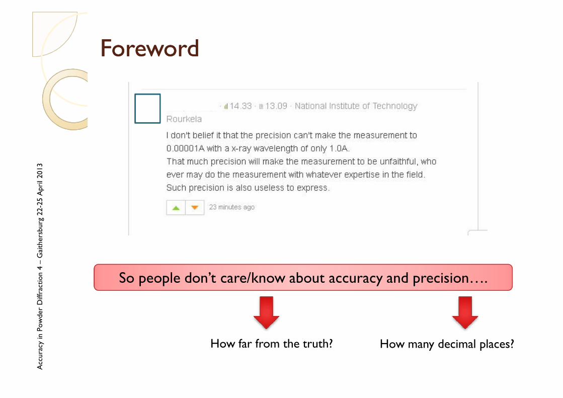
ForewordForeword
So people don’t care/know about accuracy and precision….
How many decimal places?How far from the truth?

Acc
urac
yin
Pow
der
Diff
ract
ion
4 –
Gai
ther
sbur
g22
-25
Apr
il20
13
AccuracyAccuracy and and microstructuremicrostructure
2θ
I
Antoine de Saint-Exupéry (1943)The little prince. Chapter 1
ACCURACY
"Frighten? Why should any one be frightened by a hat?”
Are you frightened by this?
Is it the right answer?

Acc
urac
yin
Pow
der
Diff
ract
ion
4 –
Gai
ther
sbur
g22
-25
Apr
il20
13
NanocrystallineNanocrystalline ceria ceria -- TEMTEM
CeO2 calcinated at 400°C for 1h
Grains are almost spherical and well separated
0 2 4 6 8 10 1205
10152025303540 TEM (average over
800 grains)
Freq
uenc
yGrain diameter (nm)
How does an XRD analysis result compare to this?

Acc
urac
yin
Pow
der
Diff
ract
ion
4 –
Gai
ther
sbur
g22
-25
Apr
il20
13
NanocrystallineNanocrystalline ceria ceria -- XRDXRD
20 40 60 80 100 120 1400
1000
2000
3000
4000
5000
6000
7000
20 40 60 80 100 120 140
100
1000
Inte
nsity
(cou
nts)
2θ (degrees)
Inte
nsity
(co
unts
)
2θ (degrees)
24h data collection on CuKα lab instrument
A high quality pattern is NEEDED to obtain accurate results

HOW DO HOW DO WEWE ANALYZEANALYZETHE DATA? THE DATA?
OLDOLDVS. VS. NEWNEW
Acc
urac
yin
Pow
der
Diff
ract
ion
4 –
Gai
ther
sbur
g22
-25
Apr
il20
13
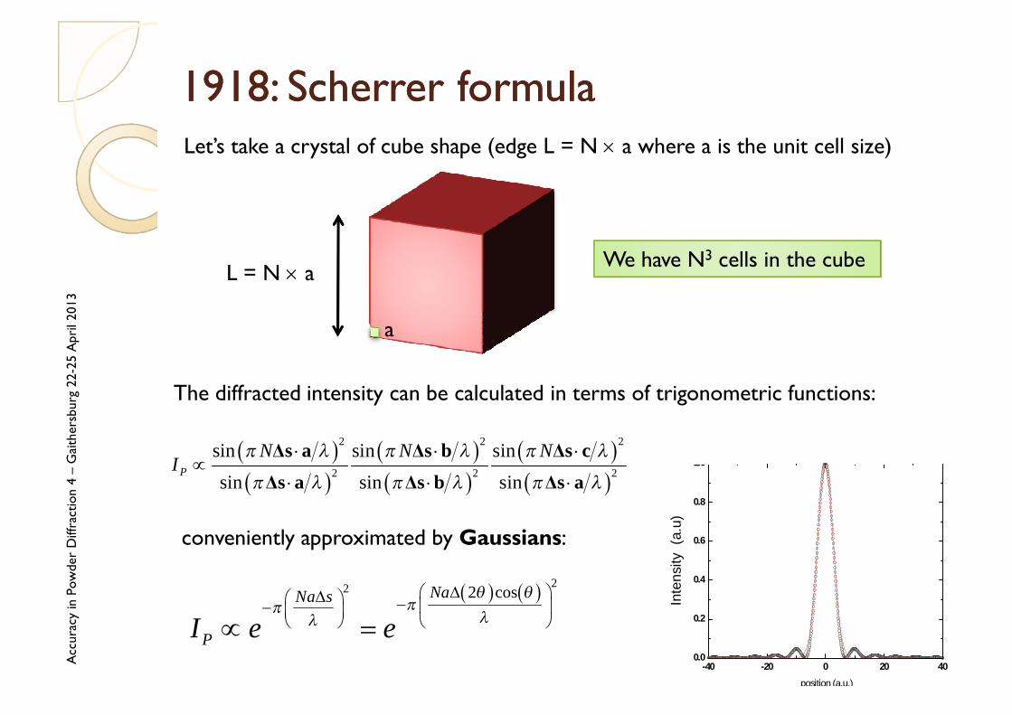
1918: Scherrer formula1918: Scherrer formulaLet’s take a crystal of cube shape (edge L = N × a where a is the unit cell size)
The diffracted intensity can be calculated in terms of trigonometric functions:
a
L = N × aWe have N3 cells in the cube
( ) ( ) 22 2 cosNaNa s
PI e eθ θ
ππ λλ
∆ ∆ − − ∝ =
-40 -20 0 20 400.0
0.2
0.4
0.6
0.8
1.0
position (a.u.)
Inte
nsity
(a.
u)
( )( )
( )( )
( )( )
2 2 2
2 2 2
sin sin sinsin sin sin
P
N N NI
π λ π λ π λ
π λ π λ π λ
⋅ ⋅ ⋅∝
⋅ ⋅ ⋅
Δs a Δs b Δs cΔs a Δs b Δs a
conveniently approximated by Gaussians:
Acc
urac
yin
Pow
der
Diff
ract
ion
4 –
Gai
ther
sbur
g22
-25
Apr
il20
13
( )
( ) ( )( )
2cos2 2 21 2
2 cos
L FWHM Lne FWHM
L
θπ
λ λ πθ
θ
⋅ −
= ⇒ =
( ) ( )0.942cos
FWHML
λθ
θ=
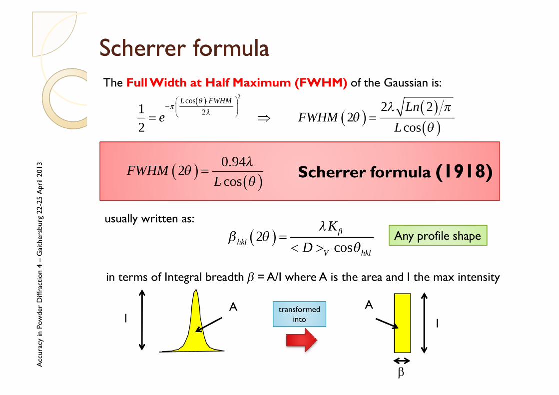
The Full Width at Half Maximum (FWHM) of the Gaussian is:
Scherrer formula (1918)
Scherrer formulaScherrer formula
usually written as:
( )2coshkl
V hkl
KD
βλβ θ
θ=
< >
in terms of Integral breadth β = A/I where A is the area and I the max intensity
IA
β
IAtransformed
into
Any profile shape

Acc
urac
yin
Pow
der
Diff
ract
ion
4 –
Gai
ther
sbur
g22
-25
Apr
il20
13
Scherrer formula (Scherrer formula (111) and (200) peaks111) and (200) peaks
25 30 35
1000
2000
3000
4000
5000
6000
7000 28.51
27.70
Inte
nsity
(co
unts
)
2θ (degrees)
29.27111
5.8VD
nmKβ
=
This is still applied by most “nanomaterials experts” in the literature
200
5.7VD
nmKβ
=
Formula obtained for GAUSSIAN/ANY peak and for a given shape of the domains (not yet decided)
Acc
urac
yin
Pow
der
Diff
ract
ion
4 –
Gai
ther
sbur
g22
-25
Apr
il20
13
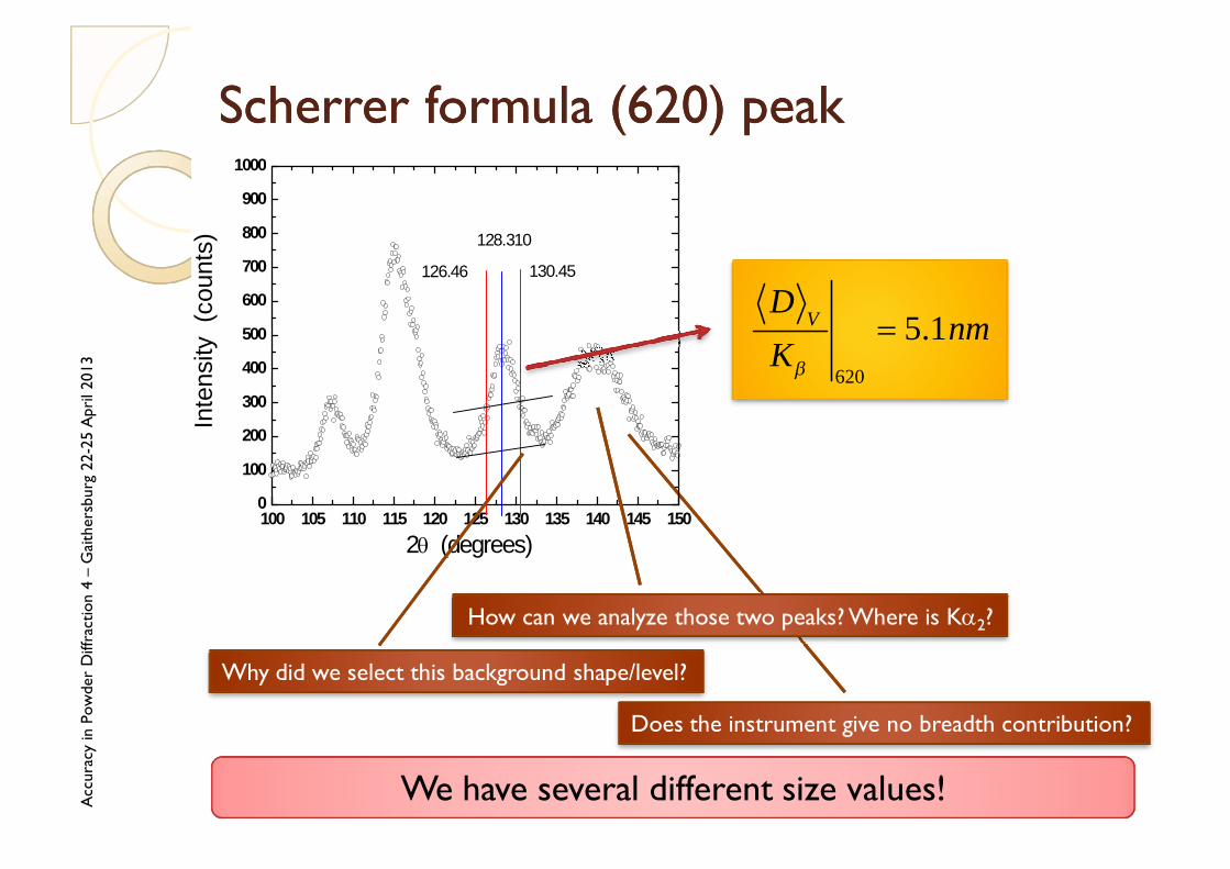
Scherrer formula (620) peakScherrer formula (620) peak
100 105 110 115 120 125 130 135 140 145 1500
100
200
300
400
500
600
700
800
900
1000
128.310
126.46
Inte
nsity
(co
unts
)
2θ (degrees)
130.45
620
5.1VDnm
Kβ
=
We have several different size values!
How can we analyze those two peaks? Where is Kα2?
Why did we select this background shape/level?
Does the instrument give no breadth contribution?

Acc
urac
yin
Pow
der
Diff
ract
ion
4 –
Gai
ther
sbur
g22
-25
Apr
il20
13
Pattern decompositionPattern decomposition
20 40 60 80 100 120 140
0
1000
2000
3000
4000
5000
6000
7000
20 40 60 80 100 120 140
100
1000
Inte
nsity
(cou
nts)
2θ (degrees)
Inte
nsity
(co
unts
)
2θ (degrees)
Use of bell-shaped functions to account for superposition
ARBITRARY bell shaped functions!

Acc
urac
yin
Pow
der
Diff
ract
ion
4 –
Gai
ther
sbur
g22
-25
Apr
il20
13
1953: Williamson1953: Williamson--Hall plotHall plot
( ) 1/2* 2 *2V
Kd d
Dββ ε= + ⋅ ⋅
Williamson-Hall plot includes Scherrer formula (1918) for “average sizedetermination” with differential of Bragg law to get information on defectspresent in the material
slope related to “microstrain”
intercept related to “average domain size”
( ) ( )0 2 sin 2 cosd dθ θ θ= ∆ + ∆ ( ) ( ) ( )2 2 tan 2 tand ed
θ θ θ∆
∆ = − = −
The β is the sum of the componentonly for Gaussian peaks
In a β(d*) vs. d* plot, intercept and slope of linear regression are related, respectively, to <D>V and e

Acc
urac
yin
Pow
der
Diff
ract
ion
4 –
Gai
ther
sbur
g22
-25
Apr
il20
13
WilliamsonWilliamson--Hall plotHall plot
( )* *2V
Kd e d
Dββ = + ⋅
< >
( )* *0.019 0.008d dβ = +
0 2 4 6 8 10 120,00
0,05
0,10
0,15
0,20
0,25
0,30
0,35
β(d*
) (n
m-1)
d* (nm-1)
“average domain size” is NOT the average size of the (nano) particles“microstrain” is a quite general term and does not identify the defect types
5.3VDnm
Kβ
< >= 0.008 0.004
2e = =

Acc
urac
yin
Pow
der
Diff
ract
ion
4 –
Gai
ther
sbur
g22
-25
Apr
il20
13
1950: 1950: WarrenWarren--AverbachAverbach methodmethodActually, in RECIPROCAL SPACE the profile is a convolution of effects!
( )( ) ( )( ) ( )( ) ( )( )size strainF h s F f s F f s F g s=
( ) ( ) ( )size strainC L A L A L=
( ) ( ) ( ) ( )size strainh s f s f s g s = ⊗ ⊗ instrument
Fourier transform
( )( ) ( )( ) ( )( )ln ln lnsize strainC L A L A L= +
We can remove the known instrumenteffects
We have a description of the profile(s) in Fourier space, from which:

Acc
urac
yin
Pow
der
Diff
ract
ion
4 –
Gai
ther
sbur
g22
-25
Apr
il20
13
WarrenWarren--AverbachAverbach methodmethod
( ) ( ) ( )( )2 2 2 2 201 2size
hklC L A L L L h aπ ε= ⋅ −
( )( ) ( )( ) ( )2 2 2 2 20ln ln 2size
hklC L A L L L h aπ ε= −
and then, taking the logarithm of both sides we obtain:
( ) ( )( )( ) ( )( )
*2
2 2 2 * 4
cos 2
1 2
strainhkl hkl
hkl hkl
A L L L d
L L d O L
π ε
π ε
=
= − +
The strain term (related to displacement between couples) can be written as:
The first order approximation for the Fourier coefficients read
Again linear plot gives size and strain contributions
Cubic case,but can begeneralised

Acc
urac
yin
Pow
der
Diff
ract
ion
4 –
Gai
ther
sbur
g22
-25
Apr
il20
13
WarrenWarren--AverbachAverbach methodmethod
( )( )ln sizeA LL=1 L=2L=3L=4
hkld⋅
hkld⋅
hkld⋅
hkld⋅
*2hkld *24 hkld
intercept gives (INDIRECTLY) the size effect
slope gives DIRECTLY the strain effect
( )( ) ( )( ) ( )2 2 2 2 20ln ln 2size
hklC L A L L L h aπ ε= −
l0
h0=1 h0=2( )( )ln C L

Acc
urac
yin
Pow
der
Diff
ract
ion
4 –
Gai
ther
sbur
g22
-25
Apr
il20
13
WarrenWarren--AverbachAverbach plotplot
0.0 0.2 0.4 0.6 0.8 1.0 1.2 1.4-3.5
-3.0
-2.5
-2.0
-1.5
-1.0
-0.5
0.0ln
(A(L
))
(d*)2 (A)
3.6S
D nm=
Taking the instrument into account, the value we obtain in much lower than the Round Robin one

Acc
urac
yin
Pow
der
Diff
ract
ion
4 –
Gai
ther
sbur
g22
-25
Apr
il20
13
WarrenWarren--AverbachAverbach methodmethodProvided that the procedure has been carried out properly (calculate FourierCoefficients, account for background, instrumental component and peakoverlapping, presence of faulting, other defects …):
( )1
22hkl Lε
( )2 2( ) sizep L d A L dL∝
( )( )hklp Lε
Size coefficients
So-called “Microstrain”
to be related to the column length distribution
to be related to the strain distribution generated by thespecific source of lattice strain)
WHICH column length distribution?Microstrain is NOT a strain!!!! WHICH source of lattice strain?

Acc
urac
yin
Pow
der
Diff
ract
ion
4 –
Gai
ther
sbur
g22
-25
Apr
il20
13
.. and for a distribution of domains
Meaning of the size termMeaning of the size term
( )p L
4 34
3
( ) ( )VV
D ML D p D dD D p D dDK M Kβ β
< >< > = = =
⋅ ∫ ∫
3 23
2
( ) ( )SS
D ML D p D dD D p D dDK M Kκ κ
< >< > = = =
⋅ ∫ ∫
D
D
L
Column length distribution…. e.g. for a single sphere:
Williamson-Hall
Warren-Averbach

Acc
urac
yin
Pow
der
Diff
ract
ion
4 –
Gai
ther
sbur
g22
-25
Apr
il20
13
Meaning of strain (distortion) termMeaning of strain (distortion) termWhen the deformation is non uniform, we can introduce the microstrain
( )1/21/2 22 d dε = ∆
ε
ε(a)
(b)
ε(c)
MICROSTRAIN is NOT a strain!!!!

Acc
urac
yin
Pow
der
Diff
ract
ion
4 –
Gai
ther
sbur
g22
-25
Apr
il20
13
Microstructure Parameters
DiffractionPattern
Instead of doing a deconvolution, we directly model the wholepattern in terms of physical models of the microstructure:
Self-consistent one-step procedure: we work on the measured data!
Structure is decoupled from microstructure, i.e. there are nostructural constraints (peak intensity is a fitting parameter).
WPPMNonlinear least
squares
Physicalmodels
2000: Whole Powder Pattern Modelling2000: Whole Powder Pattern Modelling

Acc
urac
yin
Pow
der
Diff
ract
ion
4 –
Gai
ther
sbur
g22
-25
Apr
il20
13
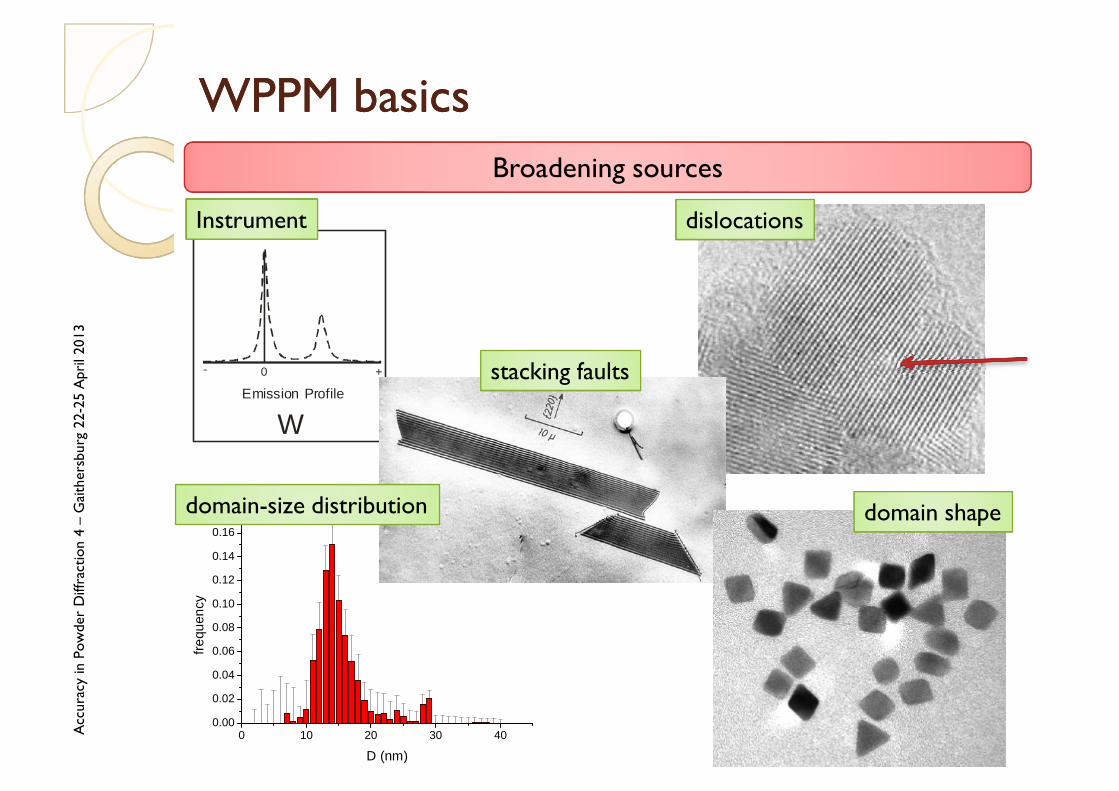
WPPM basicsWPPM basicsPattern as sum of broadened peaks + background + …
…a kind of “Pawley” or “Rietveld-like” approach… BUT….
2 0 3 0 4 0 5 0 6 02 θ (d e g re e s )

Acc
urac
yin
Pow
der
Diff
ract
ion
4 –
Gai
ther
sbur
g22
-25
Apr
il20
13
WPPM basicsWPPM basics
2θ space(diffraction peak)
reciprocal space(diffraction peak)
Each profile synthesised (in reciprocal space) from its Fouriertransform calculated by physical modelling of all broadening sources
Fourier space(complex Fourier profile)
Fourier transform Space remapping
( )C L ... we use the Warren-Averbach trick...
Acc
urac
yin
Pow
der
Diff
ract
ion
4 –
Gai
ther
sbur
g22
-25
Apr
il20
13
WPPM basicsWPPM basics
Emission Profile
- 0 +
W
Broadening sources
Instrument dislocations
stacking faults
0 10 20 30 400.00
0.02
0.04
0.06
0.08
0.10
0.12
0.14
0.16
0.18
frequ
ency
D (nm)
domain-size distribution domain shape

Acc
urac
yin
Pow
der
Diff
ract
ion
4 –
Gai
ther
sbur
g22
-25
Apr
il20
13
WPPM: plug and playWPPM: plug and play
{ } { }( ) ( ) ( )* * *, ( )exp 2hkl hkl hklhkl hklhkl
I d d k d w L iL s dLπ∞
−∞
= ⋅ ⋅∑ ∫ £
Instrumental ProfileInstrumental Profile
Domain sizeDomain size
FaultingFaulting APBAPB
DislocationsDislocations
Additional line broadening sources can be included through the corresponding FTs
{ } { } { }( ) ( ) ( ) ...IP S D F F APB GSR GSR CF CFpV hkl hkl hkl hkl hkl hklhkl hkl hklT A A A iB A A iB A iB ⋅ ⋅ ⋅ + ⋅ ⋅ + ⋅ + ⋅
Stoichiometry fluctuationsStoichiometry fluctuations
Grain surface relaxationGrain surface relaxation
The intensity is obtained as Fourier transform of the global broadening function:
Profile in recprocal space Profile in Fourier space
We have a fingerprint of the microstructure

Acc
urac
yin
Pow
der
Diff
ract
ion
4 –
Gai
ther
sbur
g22
-25
Apr
il20
13
Wilkens model for dislocation-related broadening extended to anysymmetry
General dislocation modelGeneral dislocation model
{ } ( ) ( ) { } ( )2
*2 2 *1 15exp ... , , ,
2D
ehkl hkl
bA L Inv E E h k l d L f L R
πρ
′= −
( )( )( ) { }
4 4 4 2 2 2 2 2 21 2 3 4 5 6
3 3 3 3 3 37 8 9 10 11 12
2 2 2 413 14 15
2
4
4 / hkl
E h E k E l E h k E k l E h l
E h k E h l E k h E k l E l h E l k
E h kl E k hl E l hk d
+ + + + + +
+ + + + + + +
+ + +
Coefficients calculated from slip system and single-crystal elasticconstants or refined on the data (in this last case the meaning of ρ iswatered down)

Acc
urac
yin
Pow
der
Diff
ract
ion
4 –
Gai
ther
sbur
g22
-25
Apr
il20
13
NanoNano CeOCeO22 -- WPPMWPPM
20 40 60 80 100 120 140
0
1000
2000
3000
4000
5000
6000
7000
Inte
nsity
(co
unts
)
2θ (degrees)
WPPM result: no Voigt or bell shaped arbitraryfunctions to model the data, 29 par, GoF 1.03
20 40 60 80 100 120 140
0
1000
2000
3000
4000
5000
6000
7000
Inte
nsity
(co
unts
)
2θ (degrees)
Pseudo-Voigt profiles to modelthe data, 70 par, GoF 1.01

Acc
urac
yin
Pow
der
Diff
ract
ion
4 –
Gai
ther
sbur
g22
-25
Apr
il20
13
NanoNano CeOCeO22 –– WPPM WPPM vsvs TEMTEM
0 2 4 6 8 10 120
5
10
15
20
25
30
35
40 TEM WPPM
Freq
uenc
y
Grain diameter (nm) ρ ≈ 1.4(9)·1016 m-2
ca. 1 dislocation every 3-4 grains
TEM
4.4D nm=We just assumed a lognormaldistribtion of spheres withdislocations on the primary slip system

Acc
urac
yin
Pow
der
Diff
ract
ion
4 –
Gai
ther
sbur
g22
-25
Apr
il20
13
CeriaCeria summarysummary
0 2 4 6 8 10 120
5
10
15
20
25
30
35
40 TEM WPPM
Freq
uenc
y
Grain diameter (nm)
4.4(2)D nm=
3.6S
D nm= WPPM
Warren-Averbach
5.3VDnm
Kβ
< >=
Williamson-Hall
5.1 5.8VD
nmKβ
= −
Scherrer

FURTHERFURTHER ACCURACYACCURACYPROBLEMSPROBLEMS

Acc
urac
yin
Pow
der
Diff
ract
ion
4 –
Gai
ther
sbur
g22
-25
Apr
il20
13
WPPM versus WPPM versus DebyeDebye equationequation
( ) ( )sincN N
iji j
I Q ∝ ⋅∑∑ r Q
N atoms
rij
i
jThe formula gives directly the powderdiffraction pattern in reciprocal space
0 5 10 15 20 25 300
20
40
60
80
100
Inte
nsity
(ato
ms2 )
Q (nm-1)
SAXS
WAXS
The Debye equation links atomic coordinates and diffraction pattern:
4 sinQ π θλ
=
SAXS is in the ideallydiluted limit
Acc
urac
yin
Pow
der
Diff
ract
ion
4 –
Gai
ther
sbur
g22
-25
Apr
il20
13
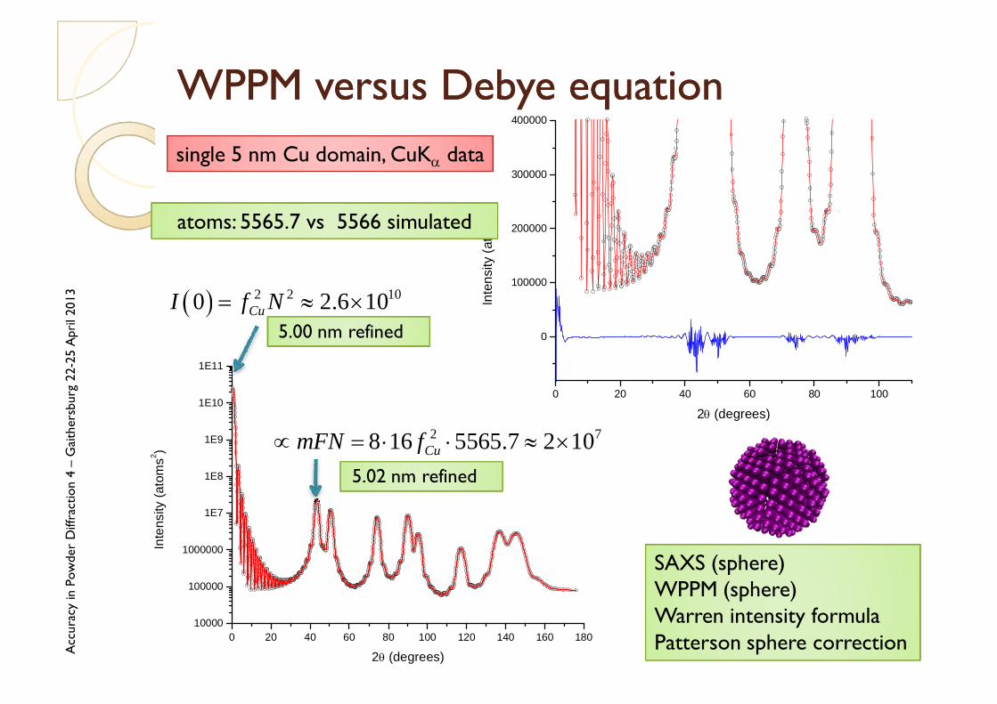
WPPM versus Debye equationWPPM versus Debye equation
0 20 40 60 80 100
0
100000
200000
300000
400000
Inte
nsity
(ato
ms2 )
2θ (degrees)
0 20 40 60 80 100 120 140 160 18010000
100000
1000000
1E7
1E8
1E9
1E10
1E11
Inte
nsity
(ato
ms2 )
2θ (degrees)
single 5 nm Cu domain, CuKα data
atoms: 5565.7 vs 5566 simulated
( ) 2 2 100 2.6 10CuI f N= ≈ ×
2 78 16 5565.7 2 10CumFN f∝ = ⋅ ⋅ ≈ ×
SAXS (sphere)WPPM (sphere)Warren intensity formulaPatterson sphere correction
5.00 nm refined
5.02 nm refined

Acc
urac
yin
Pow
der
Diff
ract
ion
4 –
Gai
ther
sbur
g22
-25
Apr
il20
13
HollowHollow 8nm Au 8nm Au spheresphere (3nm (3nm holehole))
2 3 4 5 6 7 8 90
10000
20000
30000
40000
50000
Inte
nsity
(ele
ctro
n un
its)
Q (nm-1)
2 3 4 5 6
100
1000
10000
Inte
nsity
(ele
ctro
n un
its)
Q (nm-1)
2 3 4 5 6 7 8 90
10000
20000
30000
40000
50000
Inte
nsity
(ele
ctro
n un
its)
d* (Å-1)
2 3 4 5 6
100
1000
10000
Inte
nsity
(ele
ctro
n un
its)
Q (Å-1)
8.01(6) nm, hole 3.07(11) nm
7.63(7) nm
Acc
urac
yin
Pow
der
Diff
ract
ion
4 –
Gai
ther
sbur
g22
-25
Apr
il20
13
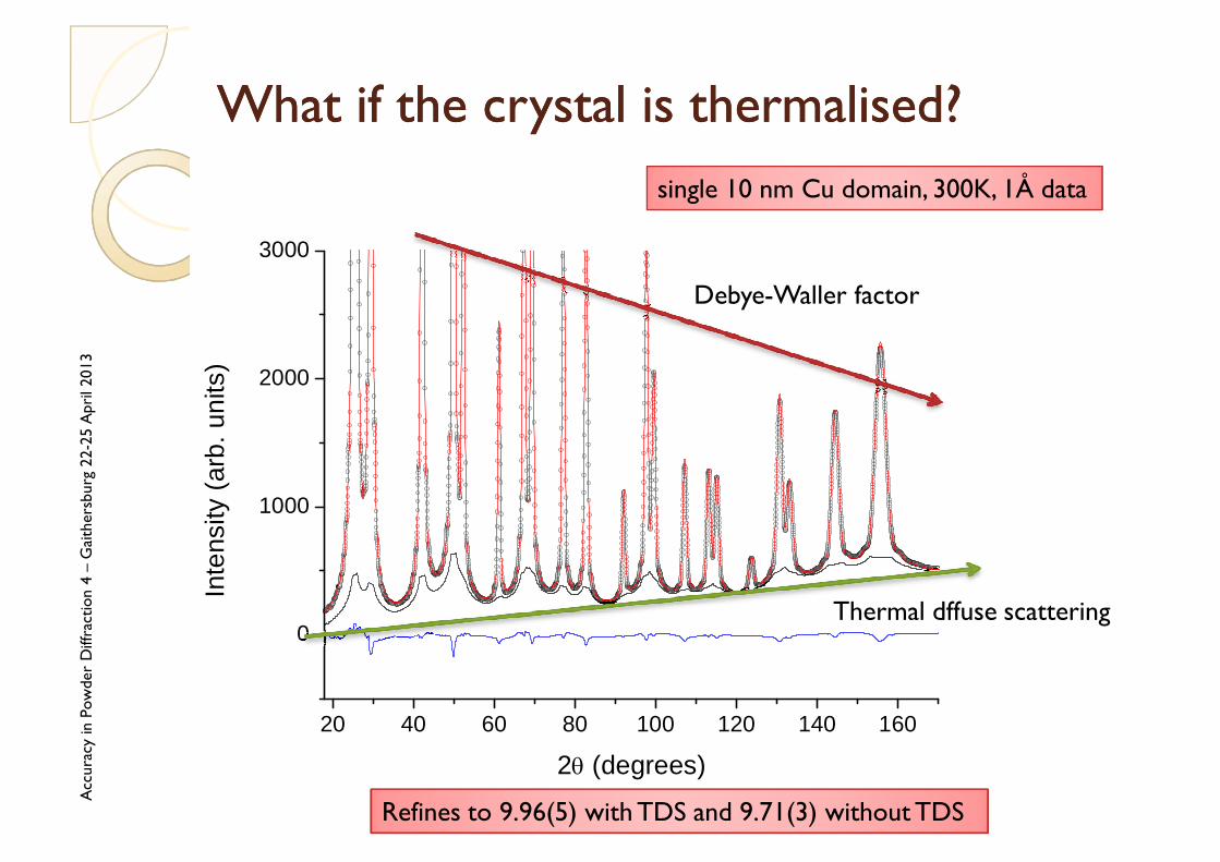
WhatWhat ifif the the crystalcrystal isis thermalisedthermalised??
20 40 60 80 100 120 140 160
0
1000
2000
3000In
tens
ity (a
rb. u
nits
)
2θ (degrees)
single 10 nm Cu domain, 300K, 1Å data
Debye-Waller factor
Thermal dffuse scattering
Refines to 9.96(5) with TDS and 9.71(3) without TDS

Acc
urac
yin
Pow
der
Diff
ract
ion
4 –
Gai
ther
sbur
g22
-25
Apr
il20
13
ProblemsProblems wihwih cellcell parameter…parameter…
Z. Kaszkur, “Nanopowder diffraction analysisbeyond the Bragg law applied to palladium”,J.Appl. Cryst. (2000). 33, 87–94

Acc
urac
yin
Pow
der
Diff
ract
ion
4 –
Gai
ther
sbur
g22
-25
Apr
il20
13
.. .. foundfound severalseveral timestimes
E. Grzanka, S.Stelmakh, C.Pantea, W.Zerda, B. Palosz, “Investigation ofthe relaxation of the nano- diamondsurface in real and reciprocalspaces”, 4-th Nanodiamond andRelated Materials jointly with 6-thDiamond and Related Films, June28th - July 1st, 2005, Zakopane,POLAND
B. Palosz, E. Grzanka, S. Gierlotka, S. Stelmakh, et al. “Diffraction studies of nanocrystals: theory and experiment.” Acta Physica Polonica Series A, 102 (2002) 57–82.
Apparent Lattice Parameter, alp

Acc
urac
yin
Pow
der
Diff
ract
ion
4 –
Gai
ther
sbur
g22
-25
Apr
il20
13
TestingTesting forfor accuracyaccuracy
40 60 80 100 120 140 1600.9985
0.9990
0.9995
1.0000
1.0005
1.0010
1.0015
2Th Degrees
alp/
a
2Th Degrees160140120100806040
Sqr
t(Cou
nts)
1.600
1.400
1.200
1.000
800
600
400
200
0
Calculation via Debye scattering formula, Cu domain 3 nm, 1202 atoms
Acc
urac
yin
Pow
der
Diff
ract
ion
4 –
Gai
ther
sbur
g22
-25
Apr
il20
13
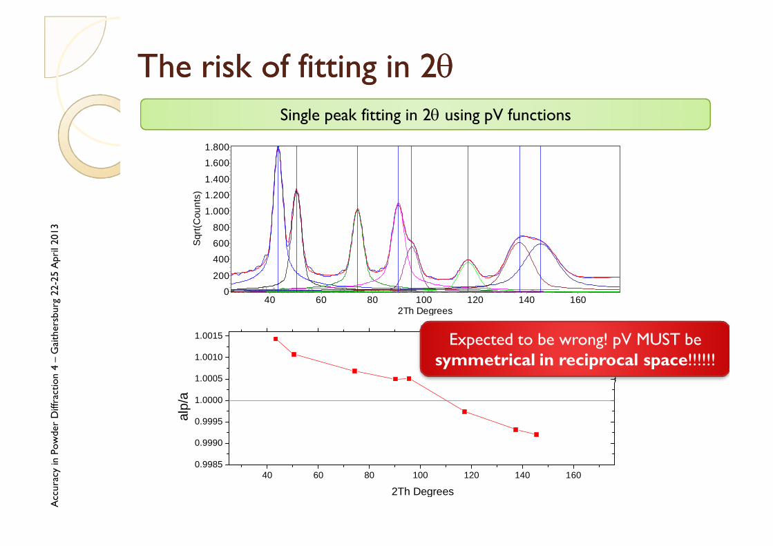
The The riskrisk ofof fittingfitting in 2in 2θθ
40 60 80 100 120 140 1600.9985
0.9990
0.9995
1.0000
1.0005
1.0010
1.0015
2Th Degrees
alp/
a
2Th Degrees160140120100806040
Sqr
t(Cou
nts)
1.800
1.600
1.400
1.200
1.000
800
600
400
200
0
Topas ©Single peak fitting in 2θ using pV functions
Expected to be wrong! pV MUST be symmetrical in reciprocal space!!!!!!

Acc
urac
yin
Pow
der
Diff
ract
ion
4 –
Gai
ther
sbur
g22
-25
Apr
il20
13
RieveldRieveld modellingmodelling: : samesame story!story!
2Th Degrees160140120100806040
Sqr
t(Cou
nts)
1.8001.6001.4001.2001.000
800600400200
0
Structure 100.00 %
Rietveld refinement using FPA considering a specimen displacement
40 60 80 100 120 140 1600.9985
0.9990
0.9995
1.0000
1.0005
1.0010
1.0015
2Th Degrees
alp/
a
Rietveld - specimen displacement = 220µm
Rietveld
Why is it wrong? First hint: pV is symmetrical in the wrong space. But not just that...

Acc
urac
yin
Pow
der
Diff
ract
ion
4 –
Gai
ther
sbur
g22
-25
Apr
il20
13
WholeWhole PowderPowder Pattern Pattern ModellingModelling
40 60 80 100 120 140 1600.9985
0.9990
0.9995
1.0000
1.0005
1.0010
1.0015
2Th Degrees
alp/
a
Rietveld - specimen displacement = 220µm
40 60 80 100 120 140 1600
200400600800
10001200140016001800
Sqrt(
Cou
nts)
2Th Degrees
WPPM
WPPM (0.999986)
Rietveld
“Ab initio” using fixed cell parameter, Patterson (1939) formula, symmetric profiles in Q, correct Lorentz factor and addition of SAXS tail
Apparent lattice parameter can therefore be an artefact!
WPPM
Acc
urac
yin
Pow
der
Diff
ract
ion
4 –
Gai
ther
sbur
g22
-25
Apr
il20
13
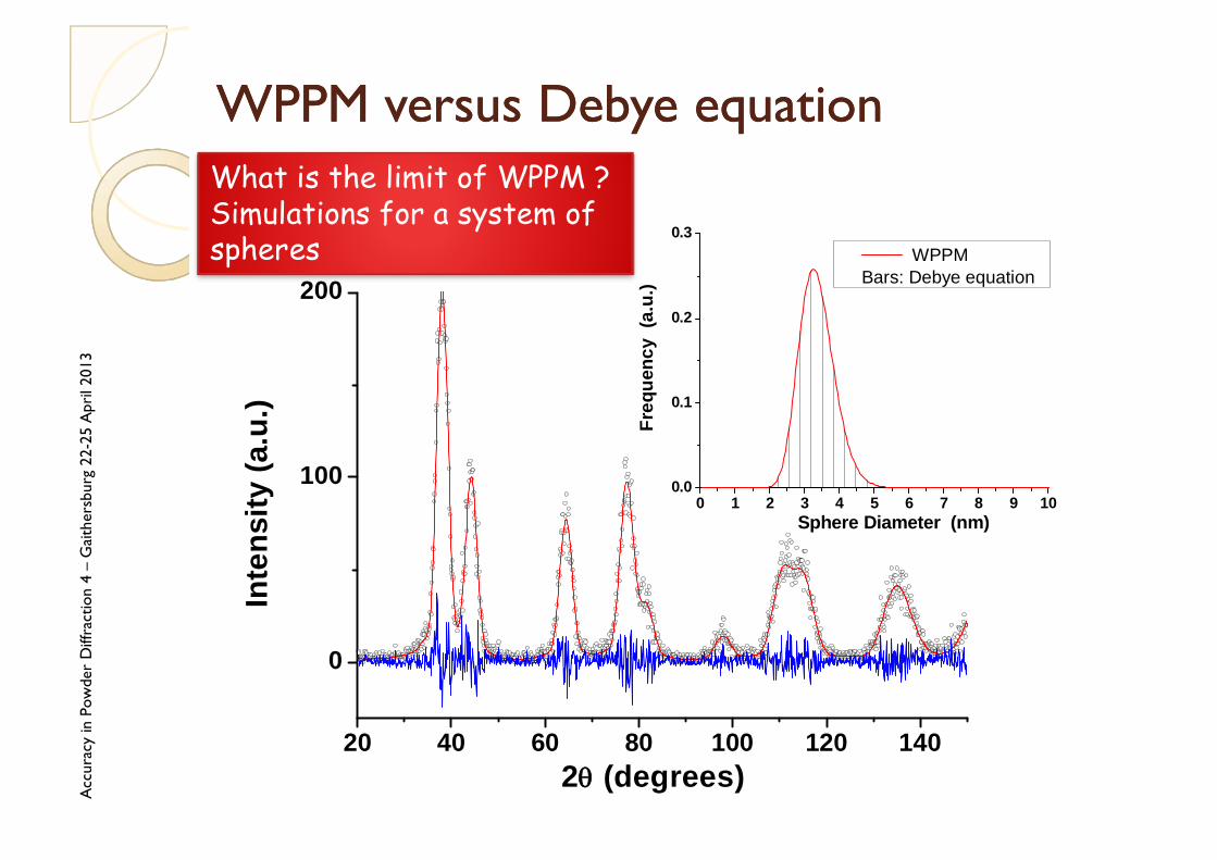
What is the limit of WPPM ? Simulations for a system of spheres
WPPM versus Debye equationWPPM versus Debye equation
20 40 60 80 100 120 140
0
100
200In
tens
ity (a
.u.)
2θ (degrees)
0 1 2 3 4 5 6 7 8 9 100.0
0.1
0.2
0.3
Freq
uenc
y (a
.u.)
Sphere Diameter (nm)
WPPMBars: Debye equation
Acc
urac
yin
Pow
der
Diff
ract
ion
4 –
Gai
ther
sbur
g22
-25
Apr
il20
13
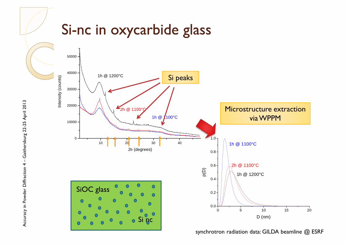
SiSi--ncnc in in oxycarbideoxycarbide glassglass
0 5 10 15 200.0
0.2
0.4
0.6
0.8
1.0
2h @ 1100°C
1h @ 1200°Cp(D
)
D (nm)
1h @ 1100°C
synchrotron radiation data: GILDA beamline @ ESRF
Microstructure extraction via WPPM
10 20 30 400
10000
20000
30000
40000
50000In
tens
ity (c
ount
s)
2θ (degrees)
2h @ 1100°C
1h @ 1100°C
1h @ 1200°C
SiOC glass
Si nc
Si peaks

EXAMPLE:EXAMPLE:CATALYSTSCATALYSTS

Acc
urac
yin
Pow
der
Diff
ract
ion
4 –
Gai
ther
sbur
g22
-25
Apr
il20
13
Au@ZrOAu@ZrO22 yolkyolk--shellshell catalystscatalysts
Complex system, hard to characterize
with the TEMImage courtesy of C. Weidenthaler, MPI fuer Kohlenforschung, Muelheim

Acc
urac
yin
Pow
der
Diff
ract
ion
4 –
Gai
ther
sbur
g22
-25
Apr
il20
13
Au@ZrOAu@ZrO22 yolkyolk--shellshell catalystscatalysts
20 40 60 80 1000
2000
4000
6000
8000
10000
Inte
nsity
(cou
nts)
2 Theta/°0 2 4 6 8 10 12 14
0.0
0.2
0.4
0.6
0.8
1.0
0 2 4 6 8 10 12 140.0
0.2
0.4
0.6
0.8
1.0
frequ
ency
(a.u
.)
D (nm)
(b)
Nanocrystalline Au inside a cage of porous
nanocrystalline ZrO2
70 m2/g
WPPM for phasesand size distribution
Phase-selectivespecific area calculation!
Acc
urac
yin
Pow
der
Diff
ract
ion
4 –
Gai
ther
sbur
g22
-25
Apr
il20
13
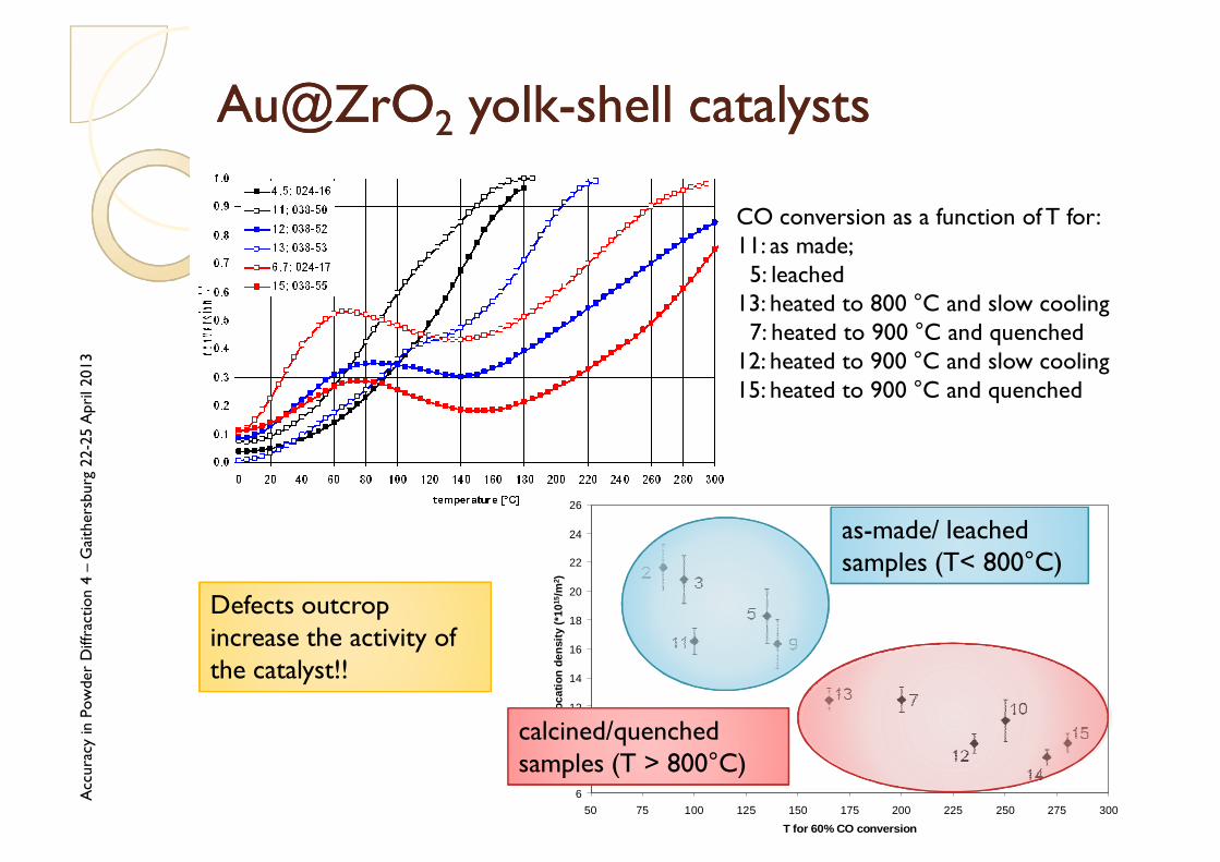
Au@ZrOAu@ZrO22 yolkyolk--shellshell catalystscatalysts
CO conversion as a function of T for:11: as made;5: leached
13: heated to 800 °C and slow cooling 7: heated to 900 °C and quenched
12: heated to 900 °C and slow cooling15: heated to 900 °C and quenched
6
8
10
12
14
16
18
20
22
24
26
50 75 100 125 150 175 200 225 250 275 300T for 60% CO conversion
disl
ocat
ion
dens
ity (*
1015
/m2 )
13
12
10
14
15
7
911
2 3
5
calcined/quenched samples (T > 800°C)
as-made/ leached samples (T< 800°C)
Defects outcropincrease the activity ofthe catalyst!!

Acc
urac
yin
Pow
der
Diff
ract
ion
4 –
Gai
ther
sbur
g22
-25
Apr
il20
13
PtPt nanocatalystsnanocatalysts
Soft chemistryemployed to control the shape of the particles
Nano-Pt by reducing H2PtCl6 using H2 in presence of sodium polyacrylate
40 60 80 100 120 140
0
2
4
6
8
10
12
14
16
Inte
nsity
(x10
3 cou
nts)
2θ (degrees)
experimental pattern calculated pattern difference
2 4 6 8 10 12 140
5
10
15
20
D (nm)
TEM octahedron tetrahedron cuboctahedron sphere
Freq
uenc
y (%
)
WPPM to check the distribution of size and shapes

CONCLUDING CONCLUDING REMARKSREMARKS
Acc
urac
yin
Pow
der
Diff
ract
ion
4 –
Gai
ther
sbur
g22
-25
Apr
il20
13
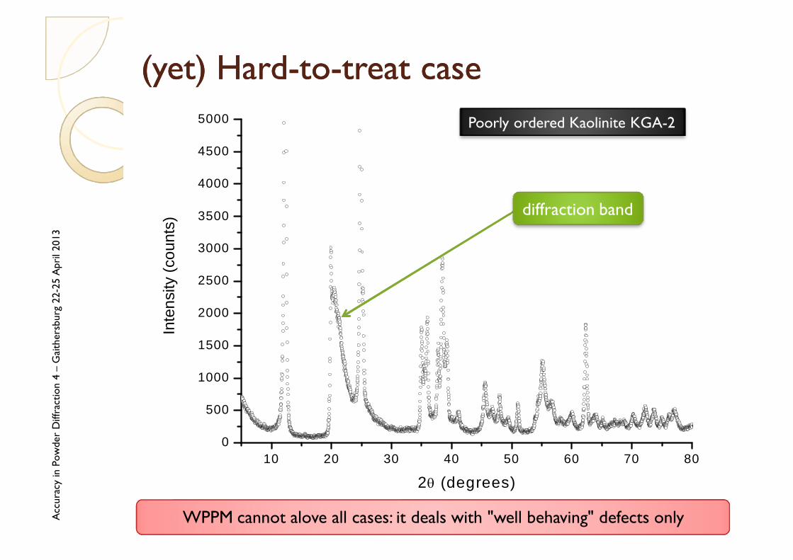
((yetyet) ) HardHard--toto--treattreat casecase
10 20 30 40 50 60 70 800
500
1000
1500
2000
2500
3000
3500
4000
4500
5000
Inte
nsity
(cou
nts)
2θ (degrees)
Poorly ordered Kaolinite KGA-2
diffraction band
WPPM cannot alove all cases: it deals with "well behaving" defects only

Acc
urac
yin
Pow
der
Diff
ract
ion
4 –
Gai
ther
sbur
g22
-25
Apr
il20
13
Concluding remarks/caveatsConcluding remarks/caveats
Accuracy in line profile analysis has definitely improved inthe last years
Use the quick and dirty tools for comparison and a WPPM-type approach for more quantitative studies
NEVER EVER use any result from microstructure analysiswithout knowing what you are doing / how you obtained it!
Fit the models on the measured data (not viceversa)
Good fit does not always mean good/accurate result

Acc
urac
yin
Pow
der
Diff
ract
ion
4 –
Gai
ther
sbur
g22
-25
Apr
il20
13
ConclusionsConclusions
2θ
I
My drawing was not a picture of a hat. It was a picture of a boa constrictor digesting an elephant. But since the grown-ups were not able to understand it, I made another drawing: I drew the inside of the boa constrictor, so that the grown-ups could see it clearly.
They always need to have things explained.