MIFIRA FrameworkLecture 12

Local supply responsiveness

Chris Barrett and Erin LentzMarch 2012

Lecture Overview

2

• What do we do when we can’t compute the degree of market integration?

• Estimate prospective equilibrium effects• Overview:

– Theoretical approach to drawing supply curves

– Example: estimate changes in demand due to transfer / procurement

– Example: estimate responsiveness of supply to change in demand, using local wholesale trader information

Supply Responsiveness

3

• Approaches to estimate equilibrium:– Link marginal costs with changes in

demand– Recover marginal costs to draw supply

curve• Marketing margins and ability to expand

– Utilize demand estimates: • Combine elasticities and MPCF and

expected size of the intervention

Price Effects of Different Supply Patterns

4Source: Barrett (2009) MIFIRA

Supply Responsiveness: Marketing Margins Revisited

• Marginal costs are often elicited as the costs associated with buying one more unit of product

• Costs vary with the number of units purchased

• How much more volume can be moved under the same marginal cost structure?

• At what volume will marketing margins increase?– By how much will the margins increase?– How much more can be moved at that margin?5

Supply Responsiveness: Discussions with traders

• Objective for discussions with traders is to learn:– Are traders at capacity?

• Room for expansion? How much?

– Do traders face barriers to expansion?– The greater traders’ capacity to

increase delivery volumes at the pre-existing price or a level near it, the greater the scope for cash-based response.

6

Supply Responsiveness: Discussions with traders

• Questions to ask traders:– If demand increases, how much more can a

trader import / sell at current prices?• If this is not concrete enough, specify demand

increase in tons or percentage

– If demand increases and prices increase by 10%, how much more can a trader sell?

– If entire stock was purchased today, how much time would a trader need to restock?

– What constrains the volume traded?

7

Supply Responsiveness: Discussions with traders

• Eliciting supply responsiveness data from traders can be difficult – Larger market actors generally have fewer

competitors• Larger actors may not be willing to participate

– Traders may have incentives to overstate their ability to meet demand

– Quite difficult to generate a statistically significant sample of major market actors • More effective to approach traders as key

informants8

Marketing Margins: Estimating Induced Price

Effects

 

Additional Marginal Volume in metric tons

Additional Procurement Cost

Additional Transportation Cost

Storage Costs

Taxes or Fees

Processing Costs

Interest or Short-term credit costs

Other Costs

Total Marginal Cost

Costs by trader

Trader 1 1.00 1900 200 12 202 100 190 0 2604

2.00 1900 450 12 202 100 190 0 2854

5.00 2500 750 0 250 100 300 0 3900

Trader 2 20.00 1900 200 12 202 100 190 0 2604

50.00 2500 500 0 250 100 200 0 3550

Trader 3 4.00 1900 200 12 202 100 190 0 2604

12.00 2000 500 15 202 100 250 0 3067

9

Marketing Margins: Estimating Induced Price

Effects

10

 Sorted volumes by Marginal costs

Total Marginal Cost

Aggregate Added Supply

Trader 1 1.00 2604 1.00

Trader 2 20.00 2604 21.00

Trader 3 4.00 2604 25.00

Trader 1 2.00 2854 27.00

Trader 3 12.00 3067 39.00

Trader 2 50.00 3550 89.00

Trader 1 5.00 3900 94.00

Estimating Marginal Costs

11Source: Barrett (2009) Food Insecurity

Demand Side

12

• Demand response– Size of the transfer, current prices– Elasticities– Marginal propensity to consume– Upper and lower bounds for sensitivity

Adding in Demand: Estimating increased volume demanded for food due to cash

distribution

13

Market

Expected Cash Dispersal

Cost of staple per metric ton

Amount of food that could be purchased with cash

Income elasticity of Demand: More elastic (closer to 1)

Income elasticity of Demand: Less elastic (further from 1)

Additional Volume demanded: High estimate

Additional Volume Demanded: Low estimate

Market A 100,000 1900 52.63 0.6 0.3 31.58 15.79

Market B 200,000 1900 105.26 0.6 0.3 63.16 31.58

Marketing Margins: Estimating Induced Price

Effects (Initial Price: 2600)

14

Income elasticity of demand scenario

Additional Supply Needed (MT)

Marginal Cost (find from ordered AS schedule)

Induced price change (%)

Scenario 1: low (0.3) market A 15.79 2604 0.2%Scenario 2: high (0.6) market A 31.58 3067 18.0%Scenario 3: low (0.3) market B 31.58 3067 18.0%Scenario 4: high (0.6) market B 63.16 3550 36.5%

Example: Estimating Rice Demand in Sirajganj

• Estimate increase in demand if cash replaced food aid in a community receiving food aid

• SHOUHARDO-MCHN program distributed 12 kilograms of wheat to each of 6500 district recipients over a single month

• The total distribution of 78 MT of wheat • Assume 1:1 substitution of rice for

wheat• IFPRI MPCs: 0.3-0.45

15

Example: Estimate rice demand in Sirajganj

 

Number of recipient house-holds (hh)

Grain given to each hh per month (kg)

Total food aid delivered per month (MT)

Marginal propensity to consume (MPC) food

Demand adjusted by MPC, per month (MT)

Sirajganj MCHN recipients 6500 12 78 0.45 35.1

Total MCHN recipients 85,000 12 1,020 0.45 459

16

…What about linking supply response to demand increases?

Source: Barrett (2009) MIFIRA

Example: Simple estimate of Sirajganj’s rice volume and

market behavior

17

• What is the level of competition at the wholesaler level?

• How diverse and numerous are upstream suppliers?

• What is current wholesaler volume?

Example: Sirajganj trader volume and ability to respond to

demand

 

Number of recipient house-holds (hh)

Grain given to each hh per month (kg)

Total food aid delivered per month (MT)

Marginal propensity to consume (MPC) food

Demand adjusted by MPC, per month (MT)

Monthly volume of largest seller in Sirajganj (MT)

Share trader would have to increase his trade volume

Sirajganj MCHN recipients 6500 12 78 0.45 35.1 148.8 0.236Total MCHN recipients 85,000 12 1,020 0.45 459 N/A N/A 

18

Source: Barrett (2009) MIFIRA

Example from Northern Kenya

19

• Estimate demand, using elicited MPCF

• Estimate supply responsiveness• Barriers to trade expansion

Example from Northern Kenya

20

• Estimating demand by eliciting MPCs in the field:– Ask likely recipient households how they would

spend a one-time gift of specified value. – Using proportional piling, households indicate

what proportion would be spent on food. – The denominator is the size of the one-time gift– The numerator is the value of the gift that

would be spent on a certain commodity.

MPCF = Amount spent on food/ Value of gift

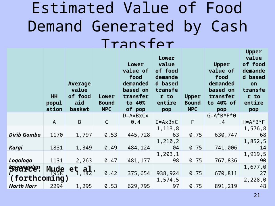
Estimated Value of Food Demand Generated by Cash

Transfer

HH popula

tion

Average value of food aid basket

Lower Bound MPC

Lower value of food

demanded based on

transfer to 40% of pop

Lower value of

food demanded

based transfer to entire pop

Upper Bound MPC

Upper value of food

demanded based on

transfer to 40% of pop

Upper value of

food demanded based on

transfer to entire pop

A B CD=AxBxCx0

.4 E=AxBxC FG=A*B*F*0.

4 H=A*B*F

Dirib Gombo 1170 1,797 0.53 445,728 1,113,863 0.75 630,747 1,576,868

Kargi 1831 1,349 0.49 484,124 1,210,204 0.75 741,006 1,852,514

Logologo 1131 2,263 0.47 481,177 1,203,198 0.75 767,836 1,919,590

Loiyangalani 1958 1,142 0.42 375,654 938,924 0.75 670,811 1,677,027

North Horr 2294 1,295 0.53 629,795 1,574,597 0.75 891,219 2,228,048

21

Source: Mude et al. (forthcoming)

Example from Northern Kenya

22

• Estimate supply responsiveness– For key commodities, what is the

trader’s maximum supply capacity at any one time given their current access to storage, transport, credit, etc., without increasing prices. ?

– All else equal, how many days does a trader need in order to fully restock?

Value of Maximum Possible Wholesale Supply Capacity of

Top 3 CommoditiesValue of

max one-off capacity per wholesaler

Max monthly restock

frequency/2

Value of max

monthly capacity per wholesaler

No of wholesalers

Total value of

wholesaler monthly capacity

Total value of current monthly

wholesaler sales

Value of Excess

capacity

A B* C=AxB D E=CxD F** G=E-F

Marsabit Town*** 4,056,250 5.0 20,281,250 10 202,812,500 21,975,000 180,837,500

Kargi 637,000 4.0 2,548,000 4 10,192,000 588,500 9,603,500

Logologo 372,125 4.0 1,488,500 2 2,977,000 529,300 2,447,700

Loiyangalani 1,024,813 4.5 4,611,659 4 18,446,634 10,284,000 8,162,634

North Horr 1,193,601 1.0 1,193,601 8 9,548,808 3,001,500 6,547,308

23

Source: Mude et al. (forthcoming)

Induced Demand for Top 3 Commodities as a Fraction of

Excess Capacity

24

Value of Excess capacity

Value of food demand generated by food basket

value income transfer to entire pop

Cash-transfer generated demand as a fraction of excess

capacity.

A B A/B*100

Marsabit Town 180,837,500 1,113,863 0.6%

Kargi 9,603,500 1,210,204 12.6%

Logologo 2,447,700 1,203,198 49.2%

Loiyangalani 8,162,634 938,924 11.5%

North Horr 6,547,308 1,574,597 24.0%

Source: Mude et al. (forthcoming)

Example from Northern Kenya

25

• Barriers to trade expansion – What would need to change for the trader

to be willing to increase his or her capacity beyond the current maximum at current sales prices?

Factors Necessary for Traders to Increase their Maximum Stocking Capacity at Current Sales Prices

26Source: Mude et al. (forthcoming)

Factors Affecting the Speed at which Extra Supply is Sources

27Source: Mude et al. (forthcoming)

Supply Responsiveness

28

• Approach:– Consider current capacity and barriers to

expansion– Elicit information on volume expansion and

cost effects, as well as barriers– Be skeptical

• examine competition, historical pricing patterns to triangulate

•Limitations of the analytic– Hypothetical situations– Marginal costs are difficult and time

consuming to elicit