Migration and the Informal Sector

Ira N. Gang (Rutgers University, RWI, GLO, CReAM, IOS, and IZA)

Melanie Khamis (Wesleyan University and IZA)

John Landon‐Lane (Rutgers University)

24 August 2017

Abstract

We study the link between temporary international migration and informal economic activity in

the home country using household level panel data from the world’s most remittance dependent

country, Tajikistan. We are interested in seeing whether migration and remittances are a substitute

for informal sector activity or a complement.

There are hosts of classifications of what constitutes informal economic activity. Our approach to

informality is grounded in a long discussion in development economics about what features are

captured and missed in survey data when one uses expenditure versus when using income. We

look at the gap between household reported income and reported expenditure. As with all surveys

there are bound to be recollection issues but we argue that a large gap between reported

expenditures and reported incomes suggests the presence of informal income.

We study the effect of migration in a causal framework on the gap. Our findings show that

households with migrants exhibit significantly lower excess expenditure over income, our measure

of informal sector activity, than non-migrant households. This holds, in particular, for remittance-

receiving households. Households with current migrants and households with several migrants

have significantly lower informal activity than non-migrant households or households that have

migrants that have already returned home for whom no migrant is currently abroad.

Migration, as a channel of income remittances, and informal sector activity are indeed substitutes

in the home country.

Key words: income, expenditure, informal, migration, remittances

JEL Codes: O17, J61, P23

Contact information: Ira N. Gang, Department of Economics, Rutgers University, 75 Hamilton

Street, New Brunswick, NJ 08901‐1248, USA, email: gang@rutgers.edu.

Melanie Khamis, Department of Economics, Wesleyan University 238 Church Street,

Middletown, CT 06459, USA, email: mkhamis@wesleyan.edu.

John Landon‐Lane, Department of Economics, Rutgers University, 75 Hamilton Street, New

Brunswick, NJ 08901‐1248, USA, email: lane@economics.rutgers.edu.

[2]

1. Introduction

This paper examines the link between temporary international migration and informal economic

activity in the home country using household level panel data. Our understanding of what

constitutes informal economic activity is very broad. Among these, it can denote employment in

enterprises that do not have access to formal capital markets or operates below some minimal

physical capital stock level. It may refer to the unmeasured economy where workers do not

formally disclose their earnings to the tax authorities. It could denote employment in small firms

with less than some small number of workers. Variants of these definitions have been used in the

literature and in this paper we do not attempt to clarify these definitions.

The informal sector plays various economic roles. For some the informal sector is bad in

the sense that workers in the informal sector are not covered by legal protections that workers in

the formal sector face (Guha-Khasnobis and Kanbur, 2006). It can be “murky” sometimes acting

as a staging ground for workers looking to advance (Fields, 1975; Gang and Gangopadhyay, 1990).

Others have shown (see for example Dimova, Gang and Landon-Lane, 2006) that the informal

sector can play a role as a safety net in periods of economic stress and crisis (Amir and Barry,

2013). The informal sector in periods of crisis can be flexible enough to quickly handle large

numbers of workers displaced from the formal sector and can help mitigate the drop in household

income that accompanies such dislocation.

This paper looks at the tradeoff between migration and informal sector activity. In

particular, we look at the role international migration and their consequent remittances have on a

household’s decision to work in the domestic (home country) informal sector. Migration,

particularly temporary migration, and remittances are typically measured and households who

send a member out of the country to work are doing so in the knowledge that the tax authorities

will see this income. We are interested in seeing whether migration and remittances are a substitute

for informal sector activity or a complement.

To do this we study Tajikistan, a country that has a very large share of its households

receiving remittances from members working outside of the country. We use an innovative

approach to measure the informal economy with household expenditure and income surveys. Our

approach is to look at the difference in household reported income and reported expenditure. As

with all surveys there are bound to be recollection issues but we argue that large differences

between reported expenditures and reported incomes suggest the presence of non-formal income.

We are confident that this gap is due to the presence of informal income as the definition of income

in the survey includes questions on consumption and savings, and consumption of household

assets. Our approach is to argue that households when reporting their income only report their

formal income – the income they reported to the authorities. However, when they report their

expenditures on the different consumption categories households do not go out of their way to

align their expenditures with their “reported” income. The benefits and issues of this approach are

[3]

related to the extensive discussion over using expenditure versus income in poverty measurement

(Deaton, 1997).

With this measure of the size of each household’s informal activity we investigate the

impact that migration has on informal sector activity. This paper considers the influence

international migration has on households’ informal sector activity as captured by the gap between

expenditure and income for households. The gap households’ face between their expenditures and

income is the subject of intrinsic interest and intensive inquiry. We push its study a bit further and

particularly want to understand the relationship between this gap and migration in a causal

framework.

Specifically, we are interested in whether migration is a substitute or a complement for

informal sector activity. That is, do households with migrants adjust their informal sector activities

or does migration with its consequent remittances occur on top of informal sector activities. Is

migration a substitute or complement for domestic economic activity? Which households are

affected and why? To close in on answers we employ a conceptual framework which begins by

thinking about what an ideal experiment would look like. Unfortunately, we do not have a lottery

or a natural experiment. Instead, we construct an alternative approach which still provides a

measure of the causal effect of migration on household informal activity as captured by the

expenditure-income difference.

Understanding the household variation in this discrepancy is key to our analysis. We are

especially interested in comparing households containing migrants to those that do not. What is it

that we are capturing when looking at the gap between expenditure and income? Many data sets

contain information on both household expenditure and income. Conceptually, if fully accounted

for they should be equal. That they are not may be a matter of recall, comfort with reporting

accurate expenditures in contrast to income, corruption, and informal sector work which frequently

goes unreported and forgotten, among other explanations. There is also difficulty with the

appropriate unit of analysis; often assignment of unreported income assumed to close the gap is to

those persons identified as working in the household, though it is really impossible to make such

an assignment. Because of this we use the household as the unit of analysis. While relevant

decisions are made jointly as well as individually, it is not possible in surveys to perfectly assign

income and expenditure individually. At minimum, there are too many joint goods.

Our strategy allows us to offer alternative interpretations of the expenditure – income gap,

for example corruption (Gorodnichenko and Peter, 2007), or the shadow economy (Torosyan and

Filer, 2014; Filer, Hanousek, and Lichard, 2015). Our approach allows the use of the rich trove of

survey data to examine the expenditure-income gap, whatever it is reflecting in household

behavior, and its links to other aspects of the economy. By examination of the discrepancy between

stated expenditures and stated income, in order to assign households to behavioral groups detailed

data on firm characteristics, social security coverage, or similar information is not needed in our

line of attack.

[4]

Our analysis shows that migration is indeed a substitute for informal sector activity.

Households actively receiving remittances have a significantly lower expenditure-income gap.

This suggests that informal sector activity is not primarily aimed at reducing the tax burden but

rather as an extra form of income needed in dire economic times.

The outline of the remainder of this paper is as follows: Section 2 provides a detailed

discussion of our measure of a household’s informal activity and background information on our

country case Tajikistan. Section 3 outlines the data used in this study. Section 4 contains our

empirical analysis and discussion while section 5 expands the analysis to numerous robustness

tests. Section 6 takes up the question of what the gap between household income and expenditure

is actually capturing. Finally, in section 7 we conclude.

2. Measuring Informal Sector Activity and Background in Tajikistan

2.1 How to Measure the Informal Sector

There is a large and growing literature on how to measure the informal sector in its various forms

and to attempt to understand its dynamics (Schneider and Enste, 2000; Maloney, 2004). In our

paper we employ household survey data from the World Bank’s Living Standard Measurement

Survey (LSMS) for Tajikistan and the similarly structured Tajikistan Household Panel Survey (see

data section below). Such surveys ask detailed questions of households about their income sources

and expenditures that we use to look for evidence of informal sector activity. The data provides

detailed information on all financial flows into and out of a household. We use this data to compute

total expenditures and total income for a household. The difference between expenditures and

households are our measure of informal sector activity. While there is bound to be measurement

and recall error in such surveys it is also normal to see very large discrepancies between reported

expenditures and reported income. It is difficult to believe that the large discrepancies are due

solely to measurement and recall error.

This approach of using the discrepancy between reported expenditures and reported

incomes was first used in Dimova et. al. (2006). In that paper the authors used the LSMS data for

Bulgaria and found significant differences between expenditures and incomes. In particular, they

found a large number of households reporting expenditures more than double the reported income.

As a check to make sure this was not pure measurement error or due to inflation of consumer prices

the authors studied households whose head was occupied in the professional sector and households

that were populated by a single person. It was found that for those households the reported

expenditures were only a few percentage points higher than the household’s reported income.

Thus, it would seem that small differences in reported expenditures and incomes could be

explained by other factors, while large deviations between reported expenditures and income

cannot be solely explained by measurement errors, recall errors or differences in the effect that

[5]

inflation has on incomes and expenditures. The literature has argued that households report

expenditures with better accuracy than income and we use this as the basis of our measure of

informal sector activity (Deaton, 1997). We argue that when faced with the detailed nature of

expenditure questions in the survey, households do not internally account for incomes they did not

report. While it is easy to only report their formal income it is hard to make sure that the amount

is reported on the expenditure side.

Moreover, the LSMS have very detailed information on all sources of income and

expenditures which allow us to make sure the discrepancy between expenditure and income is not

due to ignoring consumption of household capital or the running down of savings. For example,

the survey data allow us to calculate a household’s total expenditure including its total expenses

on goods and services, the market value of in-kind goods and services and assets consumed, and

asset accumulation (savings). Included in total household income are earnings (both in-kind and

regular), net transfers from government agencies, remittances from household members, the

market value of in-kind goods and services and assets consumed. For each household in our

estimations monthly equivalents are used for all income and expenditure variables. Home

production or the lack of measuring home production is accounted for here in that the market value

of home production (e.g. growing and eating your own food) is included in both expenditures and

income. Changes in a household’s asset stock are also accounted for in income so that any

discrepancy between expenditure and income is not due to the consumption of capital (eating the

household cow) or the running down of savings.

We have carefully used responses to properly account for non-market consumption and

income and are confident that the resulting discrepancy between reported expenditures and

reported incomes are a good indicator of unreported activity. A significant proportion of this

unreported activity is informal sector activity. Our empirical strategy utilizes the changes in the

difference between expenditures and incomes as a way of measuring the impact migration has on

informal sector activity. Since remittances are measured and hence included in income we can use

the change in the discrepancy between expenditures and incomes across households with

remittances and without remittances as a way to test whether remittances are a substitute or a

complement to informal sector activities. If we see no difference in the expenditure/income

discrepancy across households with and without remittance income, then temporary migration is

a complement to informal sector activity. If we see a decline in the expenditure/income

discrepancy for households with remittance income compared to households without remittance

income, then this is evidence that temporary migration is a substitute for informal sector economic

activity. It would also be evidence in favor of the argument that informal sector acts as a buffer

when times are bad: in bad times we expect income and expenditure to fall, but the latter not as

much. Finally, it would also be indirect evidence that the expenditure/income discrepancy is indeed

measuring informal activity rather than illegal activity as we would not expect a big change in the

expenditure/income discrepancy if the discrepancy was due to illegal or illicit activity.

We next describe the background in the context of Tajikistan, thereafter the data used in

[6]

this paper and our empirical methodology.

2.2 Background on Tajikistan

Our empirical work examines international migration and the expenditure-income gap for

Tajikistan. More than half of its 2012 GDP came from the 37% of its labor force working abroad,

making it the world’s most remittance dependent country. Estimates are that informal activity

makes up half of nonagricultural employment and that in 2006 61% of GDP was from the shadow

economy. We study Tajikistan, a poor former Soviet Republic located in Central Asia. Tajikistan

suffered severe economic, social and political changes following the USSR’s collapse. The

breakup of the Soviet Union ruptured economic ties. A civil war among rival regional clans from

1992 to 1997 was followed by an initially tenuous peace. By 1997 GDP had fallen to 35% of its

1990 level and inflation was at 65.2% (World Bank, 2011). Soon after the peace agreement and

formation of the joint government in 1997, new economic policies were put in place. Annual real

GDP grew at an 8.8% average rate from 2001-2010; average annual inflation was 20.7% (World

Bank, 2015). Even with these successes, Tajikistan is still economically trailing other former

USSR countries, having the worse poverty rate and lowest GDP per capita. GDP per capita was

US$820 in 2010 (for comparison, in the Russian Federation – US$10,481); poverty by the

headcount ratio was 47.2% in 2009 (World Bank, 2015). Compared to Russia in 2010 average

monthly wages in Tajikistan were approximately 8.5 times lower (US$82.90, Statistical

Committee of CIS, 2011). Half of the working population of Tajikistan were employed in the

traditional parts of the economy – agriculture, forestry and fisheries – where monthly wages were

US$23.60, $39.10 and $41.60, respectively (Statistical Agency of Tajikistan, 2011).

During the 2000’s there has large scale migration of Tajikistan’s labor force, mainly to

large urban areas in Russia, with more than 50% going to Moscow.1 Driven by large income and

wage differentials, migration is largely seasonal and circular the median migration spell is about 7

months (Danzer, Dietz & Gatskova, 2013a) and only one-fifth of migrants stay abroad for over

one year (Marat 2009). Tajiki migrants in the destination economy mainly work in low-skilled

jobs in trade, services and construction. Typically, they work with other Tajiki’s in jobs that are

not attractive to natives (Marat, 2009). Their remittances home are critical to Tajikistan’s

economy. 78% living abroad remit, while 99% of returning migrants bring money home (THPS

2011). These remittances are used for basic necessities such as food, house renovations and

celebrations such as weddings (THPS 2011). Very little is used to further schooling or household

enterprises or businesses (Danzer, Dietz & Gatskova, 2013a).

1 Abdulloev, Gang and Yun (2014) study the impact of massive migration on the domestic labor market in

Tajikistan. See also Abdulloev, Gang and Landon-Lane (2012) and Ivlevs (2016).

[7]

3. Data and Empirical Methodology

3.1 Data

The data that we use in this paper are the 2007 and 2009 World Bank Living Standard

Measurement Survey on Tajikistan2 (TLSS) and the 2011 Tajikistan Household Panel Survey

(Danzer, Dietz and Gatskova, 2013). The three years of data permit analysis of a panel. The 2007

TLSS interviewed 4860 households asking about schooling, well-being, employment and

migration experience. A subsample of 1503 households were re-interviewed in 2009, while 1458

of the 2009 sample were included in the 2011 sample (Danzer et al. 2013b). The panel was created

by starting with the 2011 households and variables, and matching the 2007 and 2009 information

to these. All questions (including many migration-related questions) from 2011 were retained.

Households and variables from the 2007 and 2009 surveys were retained only if included in the

2011 wave. Year-to-year panel attrition was small. From 2009 to 2011 only 45 households were

lost in the main sample, indicating that despite the large in- and outflows of family members the

core of the household was stable. The surveys are especially useful to us for they contain detailed

information on resource flow into and out of households. As noted in Section 2 the income and

expenditure variables include payments in kind and the running down of savings and the

consumption of assets. Both income and expenditure variables are converted to monthly

equivalents for each household and it is natural logarithm of the ratio of expenditure to income

that is used in our analysis.

The dependent variable in our empirical work is the natural logarithm of the ratio of

reported expenditures to reported income. Remittances from household members are included in

income. Both expenditures and income variables are from self-reported information and include

in-kind goods and services. Critical for this paper are the households whose income is less than

expenditures. Looking at the sample means it is clear that this gap is largest for households without

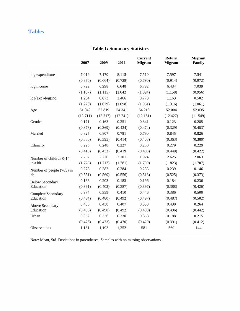
any migrants, suggesting that migrant remittances make up at least part of the gap. Looking at

log(exp)-log(inc) in Table 1, this is 1.294 in 2007, 0.873 in 2009, and 1.466 in 2011. Unreported

income is quite large in Tajikistan.

In order to examine the varying household states with respect to international migration,

we set up several different groups of migrants and non-migrants and assign households to them

(Antman, 2015). We consider three different measures of a household having a migrant. We look

2 For a detailed description of the TLSS 2007 sampling procedure see the basic information document of

the survey: http://microdata.worldbank.org/index.php/catalog/72/related_materials. The survey data is

based on a representative probability sampling on: (a) Tajikistan as a whole; (b) total urban and total rural

areas, and (c) five main administrative regions (oblasts) of the country: Dushanbe (the capital), Regions of

Republican Subordination (RRS), Sogd Oblast, Khatlon Oblast, and Gorno-Badakhshan Autonomous

Oblast (GBAO).

[8]

at households who currently have a member who is currently abroad, we look at households who

have a recently returned migrant, and we look at households that either currently have a migrant

abroad or recently returned migrant. We label the last group as migrant families. These are our

three characterizations of household’s who have participated in international migration. To have

a complete set of all possible household’s migration status, we also will identify households with

no international migration experience.

In addition to migration status we quantify a number of household characteristics. We

measure the age of the head of household, the gender of the head, the education of the head, how

many members of the household are below 15 and how many are above 65. We also include

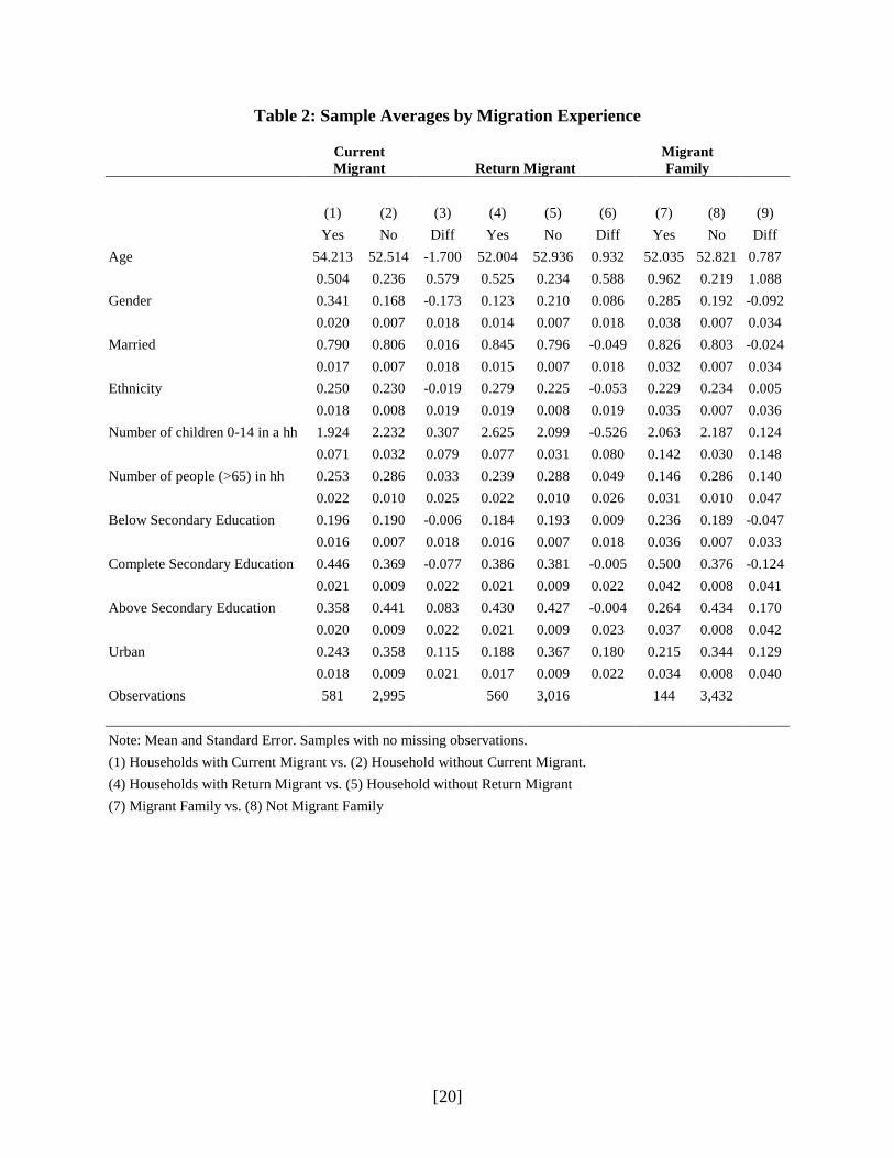
ethnicity, marital status and the location the household resides (urban or rural). Summary statistics

for these variables can be found in Tables 1 and 2. In Table 1 we report sample averages by wave

and by migration experience. In Table 2 we report sample averages by migration experience.

Figure 1 shows the kernel densities of log expenditure and log income by wave year and

by migrant status. Looking at the graphs, the distribution of income is to the left of that of

expenditure. While the distributions overlap, there are a considerable number of households with

significantly higher reported expenditures than income.

Across the first row we have plotted these kernel densities by the different surveys years,

2007, 2009 and 2011. What becomes apparent is that across all years, the same pattern exists:

expenditure is higher than income.

In the next four figures (the middle row plus the first figure in the third row) looks at

households with differing migrant status. The kernel density of expenditure is always, albeit with

varying degree, towards the right hand side of the kernel density of the distribution of income.

One could conclude that this pattern may be only visible in households with migrants and

for this reason, we also look at households with no migration experience, the middle graph in the

third row. Here, also we find that expenditure is higher than income, given the kernel densities.

For this reason, we also compare the kernel densities for expenditure and income by households

with migration experience and no migration experience at all (bottom right figure). It is apparent

from these that the migrant distribution is slightly to the left of the non-migrant distribution. When

compared to households that have no migration experience, migrant households have bother higher

mean income and expenditures.

The significance of the relationship of migration and the expenditure-income gap is a

question, as we also find this gap in general for non-migration households. In our empirical section,

we aim to test for this relationship.

[9]

3.2 Empirical Methodology

Here we sketch our estimation strategy and the thinking that lies behind it. We draw on the work

by Antman (2015), who studies the impact that emigration by male household heads from Mexico

to the United States has on intra-household allocation and distribution in Mexico. The emigrations

we consider are not necessarily male nor are they strictly by household heads. We also account

for differential impacts of current in contrast to recently returned migrants.

We want to understand the effects of migration on the difference between expenditure and

income for the household. To pin this down we first think in terms of an ideal experiment, that is,

a lottery or some random shock to the economy that would randomly provide an incentive for

some households or members of some households for migration while for other households no one

migrates. In this experiment one could take the difference between migrant households’

expenditure and income and the respective calculation for households without migrants as an

estimate of the causal effect of migration on the expenditure-income difference. Unfortunately, as

we do not have a lottery (Gibson et al. 2011) or a random shock such as a quasi-experiment or a

Mariel-type-boatlift (Card, 1990) to create an experimental setup that randomly assigns

households into treatment and control groups, we cannot just calculate this difference and conclude

that we have an unbiased causal estimate of the effect of migration.

There are several problems with such a non-randomized set-up. First, we may have

selection bias. Households that send migrants might select into migration according to unobserved

factors that may also affect income and expenditure and thereby affecting our informal sector

measure of the log ratio of expenditure and income. Second, confounding factors may be an issue

as households that send migrants might be systematically different than non-migrant sending

households, e.g. in terms of education, age etc. This could be a concern if it affects migrant sending

households differentially than non-migrant sending households. These confounding factors can be

observable and unobservable. We can control for the observable ones. Third, in the case of our

panel we may have differential effects across the three waves. Households may experience

different shocks over time and therefore adjust their expenditures. This would not necessarily be

adjusted for by our different household comparisons groups estimation, or by fixed effects

estimation. We can include year dummies to control for this potential. And finally there is a

remittances issue. The consideration of remittances is often problematic as it is often not clear who

is actually sending the remittances, and there are questions about their form and timing. We

account for remittances in a robustness check of our results.

The hypothetical experiment outlined above can provide us with an identification strategy.

It allows us to create, step-by-step as in Antman (2015), a model measuring the effect of migration

on the difference between a household’s expenditure and income and to interpret the coefficient

on migrants as a potentially causal effect of migration. We use the log ratio of expenditure to

income as the dependent variable.

[10]

To start with we select the sample of households having migration experience, whether a

currently abroad or a returned migrant or both present in the family. This way we are able to

account for self-selection based on unobserved factors that might have led to migration and that

may be correlated with our excess expenditure over income measure. Initially our sample includes

three groups of households which either have migrants currently abroad or with returned migrants

or have a combination of both present in the household, but we do not include households that

have no migrants or migration experience. In other words, here we are looking at the universe of

households who are currently or in the past had a member who migrated abroad.

Our cross-section model is, with no control variables:

0 1it it itY CurrMig , (1a)

0 1it it itY ReturnMig , (1b)

0 1it it itY MigrantFamily , (1c)

where itY is the dependent variable log expenditure minus log income, our measure of the informal

sector.

For equation 1a, the independent variable is itCurrMig and takes the value 1 if the

household has migrants currently abroad and value 0 if the household has returned

migrants/households with any migration experience (but no current migrant). The index i is the

household and the index t is the survey year (2007, 2009, 2011). Then 1 is the main coefficient

that we are interested in and would tell us the effect of having a current migrant abroad on the gap

(or for equation 1b and 1c this differs). As we are comparing current migrant households to other

migrant households the issues of selection into migration based on unobservable characteristics

may be of lesser importance as we only look at the universe of migration. This is because we are

comparing only households that have selected into migration (this is our universe, initially) and

we estimate within them the difference between having currently abroad, already returned migrants

( itReturnMig ) or having both types of migrants, returned and current migrant in the household (

itMigrantFamily ). Equations (1b) and (1c) estimate the effect of itReturnMig and

itMigrantFamily on itY , the informal sector outcome variable, within the universe of migrant

households.

Once we have tested how different forms of migration within a household affect the

informal sector we also need to consider the universe of non-migrants.

Restating from above, we think about a set-up where there are four groups of households

covering the migrant universe and the non-migrant universe:

[11]

(a) Households with migrants abroad ( itCurrMig ).

(b) Households with migrants returned (itReturnMig ).

(c) Households with migrants abroad and returned migrants (itMigrantFamily ).

(d) Household with no migration experience.

The advantage with this model is that we can use the full sample, including not only

households with migrants abroad, households with returned migrants, those with migrants both

abroad and returned but also households that have no migrants. This can add to our estimation, as

we were able to estimate the difference within migrant universe households and non-migrant

households. We combine (1a), (1b) and (1c) into equation (2) and now no-migrants form the

omitted category:

0 1 2 3it it it it itY CurrMig ReturnMig MigrantFamily . (2)

This empirical strategy provides us with a comparison of the different groups. Issues of

migration selection and confounding factors might be still there, so we include covariates to control

for observable confounding factors (equation (3)) and also household fixed effects regressions

(equation (4)),

0 1 2 3it it it it it itY CurrMig ReturnMig MigrantFamily X . (3)

The variables that make up itX are additional controls such as age, gender of the household head,

ethnicity of the household head, location of household (urban), education level of the household

head, number of children under age of 15 and number of household members over 65 and

remittances.

Cross-sectional regressions are implemented on three waves of panel with cluster standard

errors at the household level. We also include household fixed effects in our regression to account

for potential unobserved household characteristics that drive migration and return migration.

0 1 2 3it it it it it i itY CurrMig ReturnMig MigrantFamily X , (4)

[12]

where i is the household specific error term which is time-invariant.

4. Empirical Results

Equations (1) through (4) were estimated using ordinary least squares with cluster robust standard

errors. Equations (1) – (3) were estimated as a pooled regression while equation (4) was estimated

as a fixed effects panel regression. In all equations the dependent variable is the natural logarithm

of the ratio of reported household expenditure to reported household income. That is,

log logit it itY Expenditure Income .

Tables 3 - 5 contain estimation results for the variants of equation (1). The population

considered in these regressions is all households with migrants. There are three groups: households

with current migrants, households with recently returned migrants, and family migrant households

(those with both current and past migration). Households with no migration experience are not

included in these regressions. This set of estimations helps to determine the difference in the

dependent variable within the migrant household universe, whereby we distinguish between

different types of migrant households.

Table 3 reports the results for equation (1a) and for equation (1a) with controls added.

Recall that equation (1a) measures the difference in the log ratio of expenditure and income across

two groups: those households who currently have a migrant abroad and those households who

instead have a recently returned migrant or both a recently returned migrant and a current migrant

abroad. The first column in Table 3 reports the simple linear regression and shows that households

with a current migrant have a significantly lower expenditure to income gap than the base group.

This result also holds up when we add controls. Controlling for age, gender, education, ethnicity,

number of children in the household, number of old-aged persons in the household we get a

difference of -0.35 log points between households with a current migrant and the base group. The

mean log ratio of expenditure to income across the three years of the sample is 1.19 which is

equivalent to a ratio of expenditure to income of approximately 3.3. Thus households with a current

migrant have on average a ratio of expenditure to income of 2.31 compared to 3.3 for the overall

group. The impact is sizeable and of the order of reported income. The final two columns of Table

3 break the sample into an urban sample and a rural sample. For the urban sample the impact of

having a current migrant is insignificant and small whilst the impact of having a current migrant

for a rural household is significant and large.

Tables 4 and 5 do the same as Table 3 except the control group are households with a

recently returned migrant (Table 4) or households with both current and a returned migrant in the

past (Table 5). In Table 4 we get consistent results that are positive and significant on the variable

itReturnMig while in Table 5 we get consistent and negative coefficients on itMigrantFamily . The

positive coefficient on itReturnMig suggests that having a current migrant is better in terms of

[13]

remittances than having a migrant in the past. Households with a returned migrant are no longer

receiving remittances and so can crowd out less informal sector income than those households who

are currently earning income abroad.

However, the most interesting comparison is between households that have some migration

experience and those households that have no migration experience. Our hypothesis is that

remittances earned by a household member working abroad substitutes for informal sector income

which implies that households with migration experience should have a lower ratio of expenditure

to income. We test this hypothesis using regression equations (2) and (3). The results from pooled

estimation for equations (2) and (3) can be found in Table 6. Column 1 of Table 6 reports the

results from estimating equation (2) which is a comparison of the expenditure/income ratio without

any controls. In columns (2) – (4) controls are added. In all regressions the base group consists of

households that have no migration experience. The estimated coefficients for the three migrant

households, itCurrMig , itReturnMig , and itMigrantFamily are all negative and significant.

Moreover, the relative magnitudes of these coefficients are in line with the reported results from

Tables 3 - 5. The biggest reduction in the expenditure to income ratio can be found in households

that contain a current migrant, either only as current migrant or in a so-called migrant family

setting. However, all households that either have a current migrant or a recently returned migrant

show a significantly lower expenditure to income ratio compared to households that have no

migration experience. The impact is quite large with households with a current member abroad

having expenditure to income ratio that is approximately 0.9 log points lower than households

without any migration experience. For example, if a household had an expenditure to income ratio

of 3 before sending a member abroad they would have an expenditure to income ratio of

approximately 1.3 while the household member is abroad. If a household has a member currently

abroad the impact on the expenditure to income ratio is also robust to whether the household is

from an urban region or a rural region. The only category that is impacted by location is households

with a recently returned migrant. In urban areas there is little difference between those households

and household who have no migrants. One reason for this might be that in urban areas living

expenses might be high enough that any savings brought back from overseas are quickly depleted

thus making households with a returned migrant similar in nature to households who never had

migration experience.

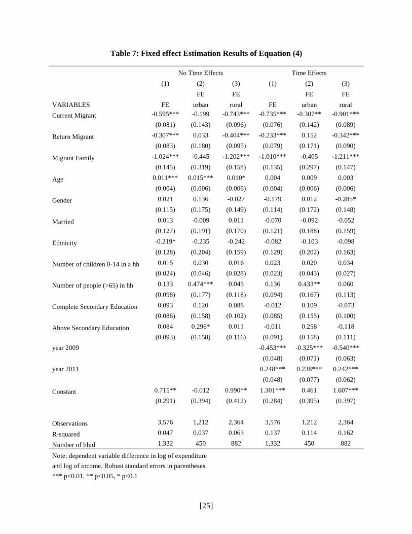
Finally, in an attempt to control for household characteristics that are both observed and

unobserved we estimate equation (4) which is to estimate a fixed effects version of equation (3).

These results can be found in Table 7. We report two sets of results for the fixed effects regressions:

one without time effects and one with time effects. As before, we find that there is a significant

impact on the natural logarithm of the ratio of expenditure to income of having a migrant currently

abroad. The coefficient is negative and significant. The magnitude varies from approximately -0.5

to -0.7 depending on whether we add time effects into the regression. Even with a value of -0.5 we

see a large drop in the ratio of expenditure to income from 3 to 1.8, a drop of more than reported

income.

[14]

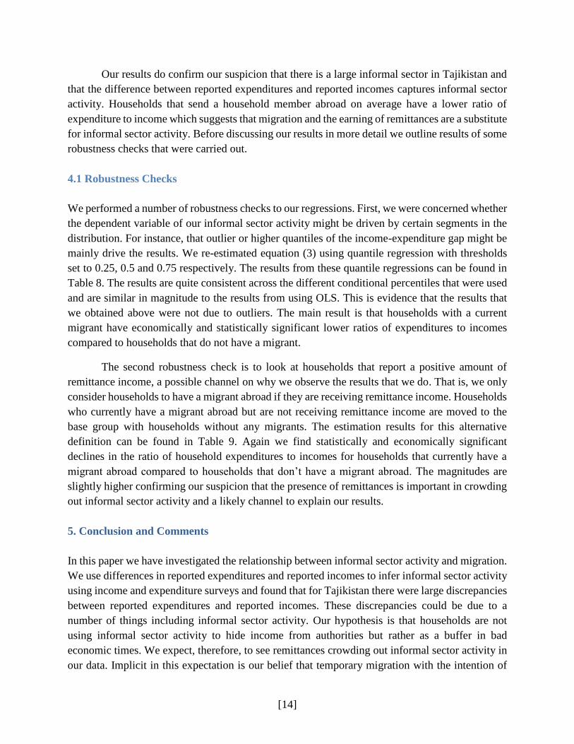
Our results do confirm our suspicion that there is a large informal sector in Tajikistan and

that the difference between reported expenditures and reported incomes captures informal sector

activity. Households that send a household member abroad on average have a lower ratio of

expenditure to income which suggests that migration and the earning of remittances are a substitute

for informal sector activity. Before discussing our results in more detail we outline results of some

robustness checks that were carried out.

4.1 Robustness Checks

We performed a number of robustness checks to our regressions. First, we were concerned whether

the dependent variable of our informal sector activity might be driven by certain segments in the

distribution. For instance, that outlier or higher quantiles of the income-expenditure gap might be

mainly drive the results. We re-estimated equation (3) using quantile regression with thresholds

set to 0.25, 0.5 and 0.75 respectively. The results from these quantile regressions can be found in

Table 8. The results are quite consistent across the different conditional percentiles that were used

and are similar in magnitude to the results from using OLS. This is evidence that the results that

we obtained above were not due to outliers. The main result is that households with a current

migrant have economically and statistically significant lower ratios of expenditures to incomes

compared to households that do not have a migrant.

The second robustness check is to look at households that report a positive amount of

remittance income, a possible channel on why we observe the results that we do. That is, we only

consider households to have a migrant abroad if they are receiving remittance income. Households

who currently have a migrant abroad but are not receiving remittance income are moved to the

base group with households without any migrants. The estimation results for this alternative

definition can be found in Table 9. Again we find statistically and economically significant

declines in the ratio of household expenditures to incomes for households that currently have a

migrant abroad compared to households that don’t have a migrant abroad. The magnitudes are

slightly higher confirming our suspicion that the presence of remittances is important in crowding

out informal sector activity and a likely channel to explain our results.

5. Conclusion and Comments

In this paper we have investigated the relationship between informal sector activity and migration.

We use differences in reported expenditures and reported incomes to infer informal sector activity

using income and expenditure surveys and found that for Tajikistan there were large discrepancies

between reported expenditures and reported incomes. These discrepancies could be due to a

number of things including informal sector activity. Our hypothesis is that households are not

using informal sector activity to hide income from authorities but rather as a buffer in bad

economic times. We expect, therefore, to see remittances crowding out informal sector activity in

our data. Implicit in this expectation is our belief that temporary migration with the intention of

[15]

earning money to be remitted back home is a substitute for informal sector activity at home. The

big difference between the two sources of income is that remittances are largely recorded while

informal sector activity is not. Under this scenario we would expect to see households with a

migrant abroad having a smaller expenditure over income discrepancy.

Using income and expenditure data from Tajikistan for the years 2007, 2009 and 2011, we

test this. These years are economically difficult years for Tajikistan and so we would expect to see

a sizeable amount of a household’s income coming from informal sector activity. In the data we

do see large discrepancies between income and expenditures with expenditures being on average

three times reported incomes over this period. Tajikistan is also interesting in that there is a very

large temporary migration out of Tajikistan and into Russia at this time. We broke the households

in the sample into households that have a current migrant, households that had a recent migrant,

households that have both a current migrant and a recent migrant, and households that have no

migration experience. In estimating the difference in excess expenditure across these households

controlling for observed and unobserved household characteristics, we find significantly lower

excess expenditure over income for households with a current migrant. The impact of migration

status on the discrepancy is large. This result is robust to a number of different specifications.

The argument put forward is that a large part of the disparity between expenditure and

income that observed in Tajikistan is informal sector activity. Also, this informal sector activity is

not an attempt to hide income but rather a safety net or buffer from difficult economic conditions.

An alternative to informal sector activity is the earning of income abroad and remitting it back.

This alternative is a substitute for informal activity. Our results show that the informal sector can

be large and can act as a buffer or safety net during difficult economic times. We also argue that

our results show that informal sector activity is not necessarily synonymous with illegal activity.

When households have a chance to earn formal income they do so and then report it.

[16]

References

Abdulloev, I., Gang, I. N., & Landon-Lane, J. (2012). Chapter 6 Migration as a Substitute for

Informal Activities: Evidence from Tajikistan, in Hartmut Lehmann, Konstantinos

Tatsiramos (ed.) Informal Employment in Emerging and Transition Economies (Research

in Labor Economics, Volume 34), Emerald Group Publishing Limited, pp.205-227.

Abdulloev, I., Gang, I. N., & Yun, M. S. (2014). "Migration, education and the gender gap in

labour force participation." The European Journal of Development Research, 26(4), pp.

509-526.

Amir, O. & Berry A. (2013). "Challenges of Transition Economies: Economic Reforms,

Emigration and Employment in Tajikistan." Social Protection, Growth and Employment

157.

Antman, F. M. (2015)."Gender discrimination in the allocation of migrant household resources."

Journal of Population Economics, 28(3), pp. 565-592.

Card, D. (1990)."The Impact of the Mariel Boatlift on the Miami Labor Market." Industrial and

Labor Relations Review, 43(2), pp. 245-257.

Danzer, A. M., Dietz, B., & Gatskova, K. (2013a). Tajikistan household panel survey: migration,

remittances and the labor market: Survey report. IOS-Regensburg. http://www.ios-

regensburg.de/fileadmin/doc/VW_Project/Booklet-TJ-web.pdf [Accessed: 05 December

2014].

Danzer, A. M., Dietz, B., & Gatskova, K. (2013b). Migration and remittances in Tajikistan: survey

technical report. http://ideas.repec.org/p/ost/wpaper/327.html [Accessed: 05 December

2014].

Deaton, A. (1997). The analysis of household surveys: a microeconometric approach to

development policy. World Bank Publications.

Dimova, R., I. Gang, and J. Landon-Lane (2006). The Informal Sector during Crisis and

Transition.in Guha-Khasnobis B. and R. Kanbur (eds) Informal Labour Markets and

Development, Palgrave-McMillan Press, 88-108.

Fields, G. (1975). "Rural-urban migration, urban unemployment and underemployment, and job-

search activity in LDCs." Journal of Development Economics, Elsevier, vol. 2(2), pp.165-

187.

Filer, R., Hanousek, J., & Lichard, T. (2015). Measuring the Shadow Economy: Endogenous

Switching Regression with Unobserved Separation (No. 10483). CEPR Discussion Papers.

Gang, I. N., & Gangopadhyay, S. (1990). "A model of the informal sector in development. "

Journal of Economic Studies, 17(5).

Gibson, J., McKenzie, D., & Stillman, S. (2011). "The Impacts of International Migration on

Remaining Household Members: Omnibus Results from a Migration Lottery Program. "

Review of Economics and Statistics, 93(4), pp. 1297-1318.

Gorodnichenko, Y., & Peter, K. S. (2007). "Public sector pay and corruption: Measuring bribery

from micro data. " Journal of Public Economics, 91(5), pp. 963-991.

Guha-Khasnobis B. and R. Kanbur (eds) (2006). Informal Labour Markets and Development,

Palgrave-McMillan Press.

Ivlevs, A. (2016). "Remittances and informal work", International Journal of Manpower, 37(7),

pp. 1172-1190.

Maloney, W. F. (2004). "Informality Revisited. " World Development, 32(7), pp. 1159–1178.

Marat, E. (2009). Labor migration in Central Asia: Implications of the global economic crisis.

[17]

Central Asia-Caucasus Institute. Silk Road Paper, May 2009.

http://www.isdp.eu/images/stories/isdp-main-pdf/2009_marat_labor-migration-in-central-

asia.pdf [Accessed 13 December 2015].

Schneider, F., & Enste, D.H. (2000). "Shadow Economies: Size, Causes, and Consequences."

Journal of Economic Literature, 38(1), pp. 77-114.

Statistical Agency of Tajikistan. (2011). Database. Retrieved September 17, 2011, from Statistical

Agency of Tajikistan: http://stat.tj/ru/database/real-sector/

Statistical Committee of CIS. (2011). Average Monthly Nominal Wage in the CIS Countries, in

national currency. Retrieved September 17, 2011, from Statistical Committee of CIS:

http://www.cisstat.com/index.html

Torosyan, K., & Filer, R. K. (2014). "Tax reform in Georgia and the size of the shadow economy.

" Economics of Transition, 22(1), pp. 179-210.

World Bank. (2011). Migration and Remittances. Factbook 2011.Second edition. Retrieved

August 12, 2011, from World Bank:

http://siteresources.worldbank.org/INTLAC/Resources/Factbook2011-Ebook.pdf

World Bank. (2015). World Data Bank. Retrieved September 17, 2011, from World Bank:

http://databank.worldbank.org/ddp/home.do?Step=12&id=4&CNO=2

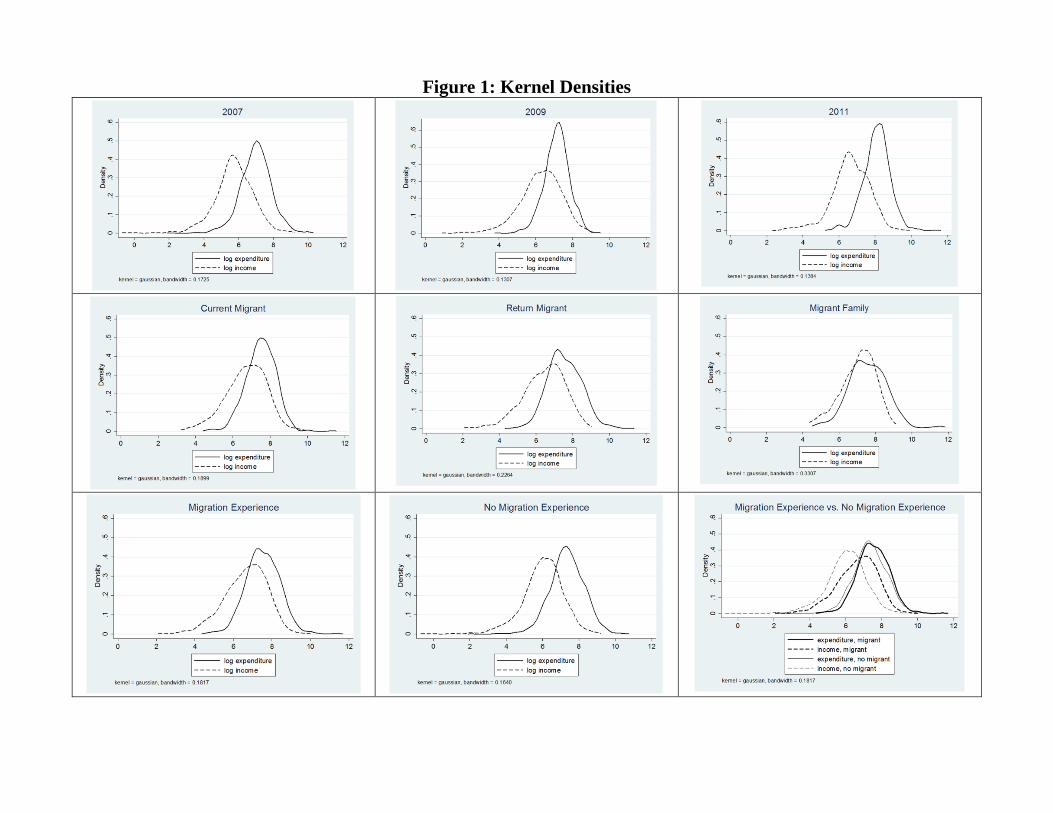
Figure 1: Kernel Densities

Tables

Table 1: Summary Statistics

2007 2009 2011

Current

Migrant

Return

Migrant

Migrant

Family

log expenditure 7.016 7.170 8.115 7.510 7.597 7.541

(0.876) (0.664) (0.729) (0.790) (0.914) (0.972)

log income 5.722 6.298 6.648 6.732 6.434 7.039

(1.167) (1.115) (1.042) (1.094) (1.158) (0.956)

log(exp)-log(inc) 1.294 0.873 1.466 0.778 1.163 0.502

(1.270) (1.079) (1.098) (1.061) (1.316) (1.061)

Age 51.042 52.819 54.341 54.213 52.004 52.035

(12.711) (12.717) (12.741) (12.151) (12.427) (11.549)

Gender 0.171 0.163 0.251 0.341 0.123 0.285

(0.376) (0.369) (0.434) (0.474) (0.329) (0.453)

Married 0.825 0.807 0.781 0.790 0.845 0.826

(0.380) (0.395) (0.414) (0.408) (0.363) (0.380)

Ethnicity 0.225 0.248 0.227 0.250 0.279 0.229

(0.418) (0.432) (0.419) (0.433) (0.449) (0.422)

Number of children 0-14

in a hh

2.232 2.220 2.101 1.924 2.625 2.063

(1.728) (1.712) (1.781) (1.700) (1.823) (1.707)

Number of people (>65) in

hh

0.275 0.282 0.284 0.253 0.239 0.146

(0.551) (0.560) (0.556) (0.518) (0.525) (0.373)

Below Secondary

Education

0.188 0.203 0.183 0.196 0.184 0.236

(0.391) (0.402) (0.387) (0.397) (0.388) (0.426)

Complete Secondary

Education

0.374 0.359 0.410 0.446 0.386 0.500

(0.484) (0.480) (0.492) (0.497) (0.487) (0.502)

Above Secondary

Education

0.438 0.438 0.407 0.358 0.430 0.264

(0.496) (0.490) (0.492) (0.480) (0.496) (0.442)

Urban 0.352 0.336 0.330 0.358 0.188 0.215

(0.478) (0.473) (0.470) (0.429) (0.391) (0.412)

Observations 1,131 1,193 1,252 581 560 144

Note: Mean, Std. Deviations in parentheses; Samples with no missing observations.

[20]

Table 2: Sample Averages by Migration Experience

Current

Migrant Return Migrant Migrant

Family

(1) (2) (3) (4) (5) (6) (7) (8) (9)

Yes No Diff Yes No Diff Yes No Diff

Age 54.213 52.514 -1.700 52.004 52.936 0.932 52.035 52.821 0.787

0.504 0.236 0.579 0.525 0.234 0.588 0.962 0.219 1.088

Gender 0.341 0.168 -0.173 0.123 0.210 0.086 0.285 0.192 -0.092

0.020 0.007 0.018 0.014 0.007 0.018 0.038 0.007 0.034

Married 0.790 0.806 0.016 0.845 0.796 -0.049 0.826 0.803 -0.024

0.017 0.007 0.018 0.015 0.007 0.018 0.032 0.007 0.034

Ethnicity 0.250 0.230 -0.019 0.279 0.225 -0.053 0.229 0.234 0.005

0.018 0.008 0.019 0.019 0.008 0.019 0.035 0.007 0.036

Number of children 0-14 in a hh 1.924 2.232 0.307 2.625 2.099 -0.526 2.063 2.187 0.124

0.071 0.032 0.079 0.077 0.031 0.080 0.142 0.030 0.148

Number of people (>65) in hh 0.253 0.286 0.033 0.239 0.288 0.049 0.146 0.286 0.140

0.022 0.010 0.025 0.022 0.010 0.026 0.031 0.010 0.047

Below Secondary Education 0.196 0.190 -0.006 0.184 0.193 0.009 0.236 0.189 -0.047

0.016 0.007 0.018 0.016 0.007 0.018 0.036 0.007 0.033

Complete Secondary Education 0.446 0.369 -0.077 0.386 0.381 -0.005 0.500 0.376 -0.124

0.021 0.009 0.022 0.021 0.009 0.022 0.042 0.008 0.041

Above Secondary Education 0.358 0.441 0.083 0.430 0.427 -0.004 0.264 0.434 0.170

0.020 0.009 0.022 0.021 0.009 0.023 0.037 0.008 0.042

Urban 0.243 0.358 0.115 0.188 0.367 0.180 0.215 0.344 0.129

0.018 0.009 0.021 0.017 0.009 0.022 0.034 0.008 0.040

Observations 581 2,995 560 3,016 144 3,432

Note: Mean and Standard Error. Samples with no missing observations.

(1) Households with Current Migrant vs. (2) Household without Current Migrant.

(4) Households with Return Migrant vs. (5) Household without Return Migrant

(7) Migrant Family vs. (8) Not Migrant Family

[21]

Table 3: Estimation Results of Equation (1a): With and without controls

(1) (2) (3) (4)

Pooled Pooled Pooled

VARIABLES Pooled controls urban rural

Current Migrant -0.241*** -0.354*** -0.196 -0.394***

(0.064) (0.066) (0.136) (0.077)

Age 0.003 -0.001 0.004

(0.004) (0.008) (0.004)

Gender -0.208** -0.289* -0.193*

(0.094) (0.164) (0.113)

Married -0.036 0.009 -0.033

(0.104) (0.182) (0.128)

Ethnicity -0.142** 0.165 -0.193***

(0.066) (0.149) (0.074)

Number of children 0-14 in a hh 0.093*** 0.064 0.098***

(0.018) (0.046) (0.019)

Number of people (>65) in hh 0.160* 0.138 0.158*

(0.085) (0.184) (0.096)

Complete Secondary Education 0.032 0.007 0.029

(0.103) (0.206) (0.119)

Above Secondary Education 0.024 -0.075 0.030

(0.107) (0.194) (0.129)

Urban 0.008

(0.076)

year 2009 -0.574*** -0.286 -0.656***

(0.090) (0.175) (0.105)

year 2011 0.209** 0.376** 0.160*

(0.082) (0.150) (0.097)

Constant 1.026*** 0.862*** 0.864* 0.885***

(0.046) (0.260) (0.511) (0.300)

Observations 1,306 1,285 277 1,008

R-squared 0.010 0.119 0.093 0.130

Note: dependent variable log difference of expenditure and income.

Robust standard errors in parentheses

*** p<0.01, ** p<0.05, * p<0.1

[22]

Table 4: Estimation Results of Equation (1b): With and without controls

(1) (2) (3) (4)

Pooled Pooled Pooled

VARIABLES Pooled controls urban rural

Return Migrant 0.438*** 0.552*** 0.406*** 0.600***

(0.066) (0.069) (0.156) (0.079)

Age 0.005 0.001 0.006

(0.004) (0.008) (0.004)

Gender -0.122 -0.209 -0.108

(0.094) (0.164) (0.113)

Married 0.026 0.029 0.048

(0.104) (0.180) (0.128)

Ethnicity -0.156** 0.140 -0.207***

(0.066) (0.145) (0.074)

Number of children 0-14 in a hh 0.080*** 0.049 0.086***

(0.018) (0.048) (0.019)

Number of people (>65) in hh 0.127 0.128 0.117

(0.085) (0.183) (0.096)

Complete Secondary Education 0.032 -0.040 0.044

(0.101) (0.202) (0.117)

Above Secondary Education -0.008 -0.117 -0.002

(0.106) (0.192) (0.128)

Urban 0.007

(0.076)

year 2009 -0.610*** -0.272 -0.715***

(0.089) (0.176) (0.104)

year 2011 0.201** 0.436*** 0.129

(0.081) (0.154) (0.095)

Constant 0.726*** 0.354 0.542 0.309

(0.040) (0.263) (0.519) (0.306)

Observations 1,306 1,285 277 1,008

R-squared 0.033 0.144 0.111 0.158

Note: dependent variable log difference of expenditure and income.

Robust standard errors in parentheses

*** p<0.01, ** p<0.05, * p<0.1

[23]

Table 5: Estimation Results of Equation (1c): With and without controls

(1) (2) (3) (4)

Pooled Pooled Pooled

VARIABLES Pooled controls urban rural

Migrant Family -0.479*** -0.395*** -0.348* -0.419***

(0.096) (0.092) (0.197) (0.106)

Age 0.001 -0.003 0.002

(0.004) (0.007) (0.004)

Gender -0.304*** -0.330** -0.306***

(0.092) (0.161) (0.111)

Married -0.079 -0.005 -0.098

(0.105) (0.178) (0.131)

Ethnicity -0.144** 0.152 -0.192**

(0.068) (0.149) (0.075)

Number of children 0-14 in a hh 0.106*** 0.077* 0.110***

(0.018) (0.044) (0.020)

Number of people (>65) in hh 0.144 0.125 0.144

(0.088) (0.186) (0.099)

Complete Secondary Education 0.000 -0.038 0.001

(0.101) (0.197) (0.118)

Above Secondary Education -0.025 -0.151 -0.002

(0.108) (0.187) (0.131)

Urban -0.003

(0.077)

year 2009 -0.494*** -0.204 -0.577***

(0.087) (0.177) (0.100)

year 2011 0.195** 0.384*** 0.144

(0.079) (0.146) (0.093)

Constant 0.971*** 0.908*** 0.932* 0.931***

(0.035) (0.263) (0.505) (0.307)

Observations 1,306 1,285 277 1,008

R-squared 0.016 0.112 0.096 0.120

Note: dependent variable log difference of expenditure and income.

Robust standard errors in parentheses

*** p<0.01, ** p<0.05, * p<0.1

[24]

Table 6: Estimation Results of Equations (2) and (3)

(1) (2) (3) (4)

Pooled Pooled Pooled

VARIABLES Pooled controls urban rural

Current Migrant -0.593*** -0.738*** -0.481*** -0.836***

(0.051) (0.052) (0.090) (0.062)

Return Migrant -0.214*** -0.238*** -0.057 -0.296***

(0.057) (0.056) (0.123) (0.063)

Migrant Family -0.885*** -0.914*** -0.695*** -1.001***

(0.092) (0.088) (0.177) (0.101)

Age 0.002 -0.001 0.003

(0.002) (0.003) (0.003)

Gender -0.012 0.081 -0.102

(0.068) (0.105) (0.087)

Married 0.003 -0.015 0.021

(0.070) (0.104) (0.095)

Ethnicity -0.162*** -0.020 -0.209***

(0.042) (0.067) (0.051)

Number of children 0-14 in a hh 0.061*** 0.053*** 0.069***

(0.011) (0.019) (0.013)

Number of people (>65) in hh 0.105** 0.125 0.092*

(0.046) (0.085) (0.055)

Complete Secondary Education 0.018 -0.073 0.036

(0.059) (0.098) (0.074)

Above Secondary Education -0.007 -0.094 0.011

(0.060) (0.095) (0.077)

Urban -0.271***

(0.041)

year 2009 -0.425*** -0.274*** -0.507***

(0.047) (0.070) (0.061)

year 2011 0.257*** 0.290*** 0.245***

(0.046) (0.070) (0.059)

Constant 1.378*** 1.321*** 1.127*** 1.337***

(0.024) (0.155) (0.226) (0.207)

Observations 3,655 3,576 1,212 2,364

R-squared 0.050 0.139 0.086 0.160

Note: dependent variable log difference of expenditure and income.

Robust standard errors in parentheses

*** p<0.01, ** p<0.05, * p<0.1

[25]

Table 7: Fixed effect Estimation Results of Equation (4)

No Time Effects Time Effects

(1) (2) (3) (1) (2) (3)

FE FE FE FE

VARIABLES FE urban rural FE urban rural

Current Migrant -0.595*** -0.199 -0.743*** -0.735*** -0.307** -0.901***

(0.081) (0.143) (0.096) (0.076) (0.142) (0.089)

Return Migrant -0.307*** 0.033 -0.404*** -0.233*** 0.152 -0.342***

(0.083) (0.180) (0.095) (0.079) (0.171) (0.090)

Migrant Family -1.024*** -0.445 -1.202*** -1.010*** -0.405 -1.211***

(0.145) (0.319) (0.158) (0.135) (0.297) (0.147)

Age 0.011*** 0.015*** 0.010* 0.004 0.009 0.003

(0.004) (0.006) (0.006) (0.004) (0.006) (0.006)

Gender 0.021 0.136 -0.027 -0.179 0.012 -0.285*

(0.115) (0.175) (0.149) (0.114) (0.172) (0.148)

Married 0.013 -0.009 0.011 -0.070 -0.092 -0.052

(0.127) (0.191) (0.170) (0.121) (0.188) (0.159)

Ethnicity -0.219* -0.235 -0.242 -0.082 -0.103 -0.098

(0.128) (0.204) (0.159) (0.129) (0.202) (0.163)

Number of children 0-14 in a hh 0.015 0.030 0.016 0.023 0.020 0.034

(0.024) (0.046) (0.028) (0.023) (0.043) (0.027)

Number of people (>65) in hh 0.133 0.474*** 0.045 0.136 0.433** 0.060

(0.098) (0.177) (0.118) (0.094) (0.167) (0.113)

Complete Secondary Education 0.093 0.120 0.088 -0.012 0.109 -0.073

(0.086) (0.158) (0.102) (0.085) (0.155) (0.100)

Above Secondary Education 0.084 0.296* 0.011 -0.011 0.258 -0.118

(0.093) (0.158) (0.116) (0.091) (0.158) (0.111)

year 2009 -0.453*** -0.325*** -0.540***

(0.048) (0.071) (0.063)

year 2011 0.248*** 0.238*** 0.242***

(0.048) (0.077) (0.062)

Constant 0.715** -0.012 0.990** 1.301*** 0.461 1.607***

(0.291) (0.394) (0.412) (0.284) (0.395) (0.397)

Observations 3,576 1,212 2,364 3,576 1,212 2,364

R-squared 0.047 0.037 0.063 0.137 0.114 0.162

Number of hhid 1,332 450 882 1,332 450 882

Note: dependent variable difference in log of expenditure

and log of income. Robust standard errors in parentheses.

*** p<0.01, ** p<0.05, * p<0.1

[26]

Table 8: Quantile Regression Results for Equation (3)

(1) (2) (3)

VARIABLES 0.25 0.5 0.75

Current Migrant -0.724*** -0.643*** -0.696***

(0.074) (0.045) (0.066)

Return Migrant -0.381*** -0.203*** 0.084

(0.078) (0.066) (0.086)

Migrant Family -0.705*** -0.819*** -0.873***

(0.098) (0.076) (0.129)

Age 0.001 0.002 0.002

(0.002) (0.002) (0.002)

Gender -0.038 0.001 0.160

(0.077) (0.085) (0.108)

Married 0.011 0.026 0.177

(0.091) (0.085) (0.112)

Ethnicity -0.125** -0.082** -0.110*

(0.055) (0.040) (0.060)

Number of children 0-14 in a hh 0.069*** 0.066*** 0.063***

(0.013) (0.011) (0.012)

Number of people (>65) in hh 0.091 0.104** 0.156***

(0.058) (0.042) (0.050)

Complete Secondary Education -0.025 -0.049 -0.017

(0.077) (0.051) (0.075)

Above Secondary Education -0.032 -0.096** -0.145**

(0.069) (0.048) (0.071)

year 2009 -0.336*** -0.357*** -0.558***

(0.073) (0.041) (0.066)

year 2011 0.388*** 0.256*** 0.021

(0.073) (0.044) (0.066)

Constant 0.536*** 1.133*** 1.772***

(0.175) (0.143) (0.196)

Observations 3,576 3,576 3,576

Note: dependent variable log difference of expenditure

and income. Standard errors in parentheses

*** p<0.01, ** p<0.05, * p<0.1

[27]

Table 9: Regression Results for Migrant Households with Remittances

(1) (2) (3) (4)

Pooled FE FE

VARIABLES Pooled controls No time effects Time effects

Current Migrant, remittance -0.692*** -0.849*** -0.698*** -0.830***

(0.051) (0.053) (0.084) (0.079)

Return Migrant -0.218*** -0.242*** -0.317*** -0.236***

(0.057) (0.056) (0.083) (0.078)

Migrant Family, Remittance -0.958*** -1.005*** -1.139*** -1.106***

(0.092) (0.088) (0.140) (0.132)

Age 0.002 0.012*** 0.005

(0.002) (0.004) (0.004)

Gender 0.024 0.062 -0.138

(0.066) (0.116) (0.115)

Married 0.038 0.013 -0.069

(0.070) (0.128) (0.121)

Ethnicity -0.155*** -0.212* -0.072

(0.042) (0.125) (0.126)

Number of children 0-14 in a hh 0.062*** 0.015 0.023

(0.011) (0.024) (0.023)

Number of people (>65) in hh 0.097** 0.131 0.132

(0.046) (0.098) (0.094)

Complete Secondary Education 0.030 0.105 0.003

(0.059) (0.086) (0.084)

Above Secondary Education 0.007 0.104 0.012

(0.059) (0.093) (0.090)

Urban -0.285***

(0.041)

year 2009 -0.427*** -0.454***

(0.047) (0.048)

year 2011 0.255*** 0.243***

(0.046) (0.048)

Constant 1.382*** 1.259*** 0.665** 1.236***

(0.024) (0.155) (0.289) (0.283)

Observations 3,655 3,576 3,576 3,576

R-squared 0.059 0.151 0.055 0.144

Note: dependent variable log difference of expenditure and income.

Robust standard errors in parentheses

*** p<0.01, ** p<0.05, * p<0.1