migration versus inversion in electromagnetic imaging

J. Geomag. Geoelectr., 49, 1415-1437, 1997

Migration versus Inversion in Electromagnetic Imaging Technique

Michael S. ZHDANOV and Peter TRAYNIN

Department of Geology and Geophysics, University of Utah, Salt Lake City, UT 84112, U.S.A.

(Received January 31, 1997; Revised August 29, 1997; Accepted September 12, 1997)

One of the most challenging problems in electromagnetic (EM) geophysical methods is developing fast and stable methods of imaging inhomogeneous underground structures using EM data. In our previous publications we developed a novel approach to this problem, using EM migration.

In this paper we demonstrate that there is a very close connection between the method of EM migration and the solution of the conventional EM inverse problem. Actually, we show that migration is an approximate inversion. It realizes the first iteration in the inversion algorithm, based on the minimization of the residual field energy flow through the profile of observations. This new theoretical result opens a way for formulating a new imaging condition. We compare this new imaging condition with the traditional one, obtained for simplified geoelectrical models of the subsurface structures.

This result also leads to the construction of a solution of the inverse EM problem, based on iterative EM migration in the frequency domain, and gradient (or conjugate gradient) search for the optimal geoelectrical model. However, the authors have found that in the framework of this method, even the first iteration, based on the migration of the residual field, generates a reasonable geoelectrical image of the subsurface structure.

1. Introduction

One of the most challenging problems in electromagnetic (EM) geophysical methods is developing fast and stable methods of imaging inhomogeneous underground structures using EM data. Solution of this problem is important for many practical applications ranging from mineral exploration to waste and building site characterization. In the papers (Zhdanov et al., 1995) and (Zhdanov et al., 1996) and the references therein we have developed a novel approach to EM imaging based on the notion of EM migration. The method includes downward continuation of the observed field or one of its components in reverse time and application of the corresponding imaging conditions. However, until recently the relationship between EM migration imaging and traditional EM inversion have remained unexplored. The conventional EM inversion means a method which predicts the geoelectrical model generating the theoretical data closed to observations. The EM migration introduced in our previous publications constructed an image of subsurface geoelectrical structures, and there was no guarantee this image, if included in a geoelectrical model, would give rise to theoretical EM fields that matched those observed.

Meanwhile, Tarantola (1987) demonstrated that seismic wave migration, which was the prototype for EM migration, can be treated exactly as the first iteration in some general wave inversion scheme. In this paper we formulate an important new result: EM migration, as the solution of the boundary value problem for the adjoint Maxwell's equation in frequency domain, can be clearly associated with the inverse problem solution. In other words, we prove that a geoelectrical model constructed on the basis of migration images would actually generate a theoretical field close to observations.

We introduce the residual EM field as the difference between the simulated EM field for some given (background) geoelectrical model and the actual EM field. The EM energy flow of the

1415

1416 M. S. ZHDANOV and P. TRAYNIN

residual field through the surface of observations can be treated as a functional of the anomalous conductivity distribution in the model. The analysis shows that the gradient of the residual field energy flow functional with respect to the perturbation of the model conductivity is equal to the integral over frequencies of the product of the incident (background) field and the migrated residual field, calculated as the solution of the boundary value problem for the adjoint Maxwell's equation.

This result clearly leads to a construction of the rigorous method of solving the inverse EM problem, based on iterative EM migration in the frequency domain, and gradient (or conjugate gradient) search for the optimal geoelectrical model. However, the authors have found that in the framework of this method, even the first iteration, based on the migration of the residual field, generates a reasonable geoelectrical image of the subsurface structure. We call the anomalous conductivity, calculated on the first iteration, the migration apparent conductivity. This new theoretical result suggests a new imaging condition formulation and indicates a new approach to EM imaging, based on iterative migration. The iterative migration forms a principally new method of interpreting EM data, which combines the ideas of downward continuation and traditional inversion. We compare this new imaging technique with the popular Rapid Relaxation Inversion (RRI) method developed by Smith and Booker (1991). Numerical modeling demonstrates that migration generates reasonable images of the subsurface structures even faster than rapid inversion.

In summary, in this paper we demonstrate that EM migration imaging can also be considered as the initial step in the general EM inversion procedure. This similarity facilitates better understanding the mathematical and physical background of EM migration, and, at the same time, develops new geoelectrical imaging tools.

For the sake of simplicity, in this paper we consider only the 2-D frequency domain geoelectrical problem. However, all the results, developed below can be generalized to the 3-D case. The solution of the 3-D migration and inversion problem is the subject of a separate paper, submitted to Geophysical Journal International (Zhdanov and Portniaguine, 1997).

2. 2-D EM Inverse Problem in the Frequency Domain

Consider a 2-D geoelectrical model with a background electrical conductivity a = ab and a local inhomogeneity D with conductivity a = ab + 6.a, varying spatially. Note that the background conductivity in general case also can be a function of coordinate ab = ab (x, z). However, it is assumed that it is known a priori. We assume that /-l = /-lo = 41f x 10-7H/m, where lio is the free-space magnetic permeability. The model is excited by an E-polarized field generated by a linear current density jex = fXd y, which is distributed in a domain Q in the upper half-plane (z ::; 0) with the constant conductivity ab (x, z::; 0) = const. Here {dx,dy,d z } is the orthonormal basis of the Cartesian system of coordinate with the origin on the earth's surface. This field is time harmonic as e- iwt . We also consider the quasi-stationary model of the EM field, so displacement currents are neglected (Zhdanov and Keller, 1994). Within this model, the EM field can be described by a single function E y satisfying the equation:

\72E y + iW/-lo C7b Ey = -iW/-lof x , z::; 0,

(1) \72E y + iW/-loC7E y = 0, z 2: 0,

and the magnetic field components can be expressed by the equations:

1 ou; H 1 ec;H ---- --- (2)x - iwlio az' z - iw /-lo ax .

1417 Migration versus Inversion

We can introduce the complex Poynting vector P as following (Stratton, 1941):

1 * 1 * 1 * P = "2E x H = "2EyHzdx - "2EyHxdz, (3)

where in the case of E-polarization E = Eydy, H* = H;dx + H;dz and * indicates a complex conjugate value. The real part of the vector P describes the intensity of the EM field energy flow. The divergence of the real part of P determines the energy dissipated in heat per unit volume per second:

\7. ReP = -~(}E. E*. (4)2

It can be shown using 2D Green's theorem that the total energy Q dissipated throughout any region S bounded by a contour L is equal to:

Q = - Re 1P . ndl = ~ JIs o E . E*ds 2: 0, (5)

where n is the unit outward normal vector and the contour is traversed counterclockwise. When the region S coincides with the lower half-plane (z 2: 0), the contour L can be composed

of the horizontal axis z = °and an infinitely large semicircle in the lower half-plane. Since the EM field satisfies to the radiation conditions, i.e., functions E and H* vanish exponentially at infinity, the contour integral over infinitely large semicircle tends to zero. Thus, the total energy Q dissipated in the lower half-plane can be calculated using the formula:

= 1 J+=Q = Re J_=+p. dzdl = -4 _= (EyH; + E;Hx) dx', (6)

where x' is the integration variable and we use the formula Re (EyH;) = ~ (EyH; + E;Hx). Let us denote the EM field components observed on the surface of the Earth (z = 0) at

the point x' as E~bs (x', 0, w), H~bs (x', 0, w) and also denote the theoretical EM field components

calculated for a given background geoelectrical model (}b (x, z) as Et (x', 0, w), H~ (x', 0, w). We can introduce the residual fields as the difference between the observed and background theoretical fields:

E:; (x',o,w) = E~bs (x',o,w) - Et (x',o,w), (7)

H;' (x',o,w) = H~bs (x',o,w) - H~ (x',o,w).

The observed field is generated by the real geoelectrical cross section a (x, z) = (}b (x, z)+~() (x, z) and actually exists everywhere in the vertical section. Therefore, the residual field can be determined everywhere as a function of coordinates (x, z) and satisfies the equations:

\72E:; + iWJ-lO(}bE:; = 0, z::; 0,

n 2 E 6. · E6. . A Eobs > 0v y + 'lwJ-lO(}b y = -'lwJ-loL..),.(} y , z _ , (8)

6. 1 1 aE:;aE:; 6.H =--- H =-

x iw J-lo az' z iw J-lo ax . The total energy flow Q6. of the residual field through the earth's surface (z = 0), is calculated

by the formula:

J+= 1 J+=Q6. = _ Re p6. . d dl = - (E6. H6.* + E6.*H6.) dx ' (9)_= z 4 -00 y x y x ,

where we use the "+" sign, opposite to the sign of the expression (6), because the sources of the residual field, excess currents in the inhomogeneity D, are located in the lower half-plane. Pankratov, Avdeev and Kuvshinov (1995) have proved an important theorem, according to which the energy flow Q6. of the residual field is non-negative:

Q6. ~ 0. (10)

Moreover, if the conductivity of the upper half-plane is assumed to be nonzero (ab > 0) the residual field energy flow is always positive (for residual field not identically equal to zero E:; =f 0). This result can be obtained from the Eq. (5) applied to the upper half-plane:

Q6. = -ab /1 Ey6. Ey6.* ds = -ab /1 IEy6.1 2 ds > 0, 1,1. Ey6. =f 0. (11)

2 z~O 2 z~O

Based on this theorem we can introduce the measure of the difference between the observed and the background theoretical fields as the residual field energy flow, integrated over the frequency range f1:

r1+00

 (ab) = rQ6.dw = ~ (E~ H:;* + E~* H:;) dx'dw. (12)in in -00

The functional (ab) can be treated as an analog of the misfit between the observed and theoretical fields. The advantage of this new functional in comparison with the traditional misfit functional is that (ab) has a clear physical meaning of the residual field energy flow through the profile of observations.

Obviously, the background theoretical field components Et (x', 0, w) and H~ (x', 0, w) depend on the conductivity distribution ab(x, z) in the given geoelectrical model and, therefore, can be treated as a functional of the conductivity model: = (ab)' We would like to modify the background conductivity in such a way that it will be equal to the actual conductivity within the anomalous domain D. In this case the new background field will be close to the observed field.

Thus, the 2-D EM inversion problem can be reduced to the minimization of the functional:

 (ab) = min. (13)

In the following section we will discuss an approach to the solution of this problem. Note that the analysis given in this section for the TE mode applies in an analogues manner

to the TM mode. It is important to notice also that similar to the case of the traditional misfit functional it is possible to incorporate measurement uncertainties in the functional given by Eq. (12) by using weighted data. In this case this functional will correspond to the energy of the weighted EM data.

3. The Steepest Descent Method of Nonlinear Inversion

We begin our analysis with the formulation of the steepest descent method of solving the minimization problem (13). The critical problem in realizing any steepest descent method is the calculation of the steepest ascent direction (or the gradient) of the functional. To solve this problem, let us perturb the background conductivity distribution: a~ (x, z) = ab (x, z) + ba (x, z). Actually, we have to perturb the conductivity only within the inhomogeneous domain D of the lower half-plane:

So (x, z) = 0, (x, z) ~ D. (14)

The first variation of the misfit functional with respect to the perturbation of the background conductivity can be calculated as:

r1+00

b (a, ba) = ~ (bE~ H:;* + E~bH:;* + bE~* H:; + E~*bH:;) dx'dw. (15)4 in -00

where we use the "+" sign, opposite to the sign of the expression (6), because the sources of the residual field, excess currents in the inhomogeneity D, are located in the lower half-plane. Pankratov, Avdeev and Kuvshinov (1995) have proved an important theorem, according to which the energy flow Q6. of the residual field is non-negative:

Q6. 2:: O. (10)

Moreover, if the conductivity of the upper half-plane is assumed to be nonzero (O"b > 0) the residual field energy flow is always positive (for residual field not identically equal to zero E~ -I- 0). This result can be obtained from the Eq. (5) applied to the upper half-plane:

Q6. = -O"b /1 Ey 6. E y 6.* ds = -O"b /1 IE y 6.1 2 ds > 0, zf. E 6. -I- o. (11)

2 z~O 2 z~O y

Based on this theorem we can introduce the measure <P of the difference between the observed and the background theoretical fields as the residual field energy flow, integrated over the frequency range 0:

<P (O"b) = { Q6.dw = ~ {J+oo (E; H;-* + E;* H;-) dx'dw. (12)in 4 in -00

The functional <P (O"b) can be treated as an analog of the misfit between the observed and theoretical fields. The advantage of this new functional in comparison with the traditional misfit functional is that <P (O"b) has a clear physical meaning of the residual field energy flow through the profile of observations.

Obviously, the background theoretical field components Et (x', 0, w) and H~ (x', 0, w) depend on the conductivity distribution O"b(X, z) in the given geoelectrical model and, therefore, = <P (O"b)' We would like to modify the background conductivity in such a way that it will be equal to the actual conductivity within the anomalous domain D. In this case the new background field will be close to the observed field.

Thus, the 2-D EM inversion problem can be reduced to the minimization of the functional:

<P (O"b) = min. (13)

In the following section we will discuss an approach to the solution of this problem. Note that the analysis given in this section for the TE mode applies in an analogues manner

to the TM mode. It is important to notice also that similar to the case of the traditional misfit functional it is possible to incorporate measurement uncertainties in the functional <P given by Eq. (12) by using weighted data. In this case this functional will correspond to the energy of the weighted EM data.

3. The Steepest Descent Method of Nonlinear Inversion

\\Te begin our analysis with the formulation of the steepest descent method of solving the minimization problem (13). The critical problem in realizing any steepest descent method is the calculation of the steepest ascent direction (or the gradient) of the functional. To solve this problem, let us perturb the background conductivity distribution: O"~ (x, z) = O"b (x, z) + 80" (x, z). Actually, we have to perturb the conductivity only within the inhomogeneous domain D of the lower half-plane:

80" (x, z) = 0, (x, z) ~ D. (14)

The first variation of the misfit functional with respect to the perturbation of the background conductivity can be calculated as:

8<p (0",80") = ~ {J+oo (8E; H;-* + E;8H;-* + 8E;* H;- + E;*8H;-) dx'dw. (15) 4 in -00

Here bE~, bH~* are the first variations of the residual electric and magnetic fields:

bE~ = 15 (E~bs (x',o,w) - Et (x',o,w)) = -bEt (x',o,w) , (16)

su> = 15 (Ho bs* (x' ° w) - H b* (x' ° w)) = -su': (x' ° w)x X " x' , X'"

using bE~bs = bH~bs* = 0. According to Appendix A the first variations of the background electric and magnetic fields

can be calculated as:

bEt (x',O,w) = iW/lo JIv C(JbbeTEtds, (17)

b (' ) bJr{ 8C a i,sn; x, 0, w = - JD ----a;;ba Eyds, (18)

where C(Jb is the Green's function of the geoelectrical model with the background conductivity eTb = eTb (x, z). Substituting Eqs. (17) and (18) into Eqs. (16) and (15) and changing the order of integration, we obtain:

bcp (o, beT) = -~ Je {So { J+oo (iW/lOC(JbEtH;* - E~ 8C~b Et* 4 JD J[2 8z-00

<uau C* E b* Hb. - Eb.* 8C(Jb E b) d 'd d (19),....,0 a i, Y X Y 8z' y x w s.

At the same time the residual magnetic field H~ can be expressed as the vertical derivative of the residual electric field E; using the equation:

b. 1 BE;H =----- (20)

x iW/lo iiz' .

Taking the last equation into account we can modify Eq. (19):

-~ Jf, So 1E b . j+oo (c 8E;b. - Eb.* 8C(Jb) d 'd dbcp (o, beT) 4 y o i, 8' y B' x W SD [2 -00 Z z

E b* 8E --1 Jf, So 1 . j+oo (C* -y-b. - Eb.~8C* ) d 'd d (21)4 y a i, 8 ' y 8' x W S.

D [2 -00 Z Z

According to Appendix B:

j +OO ( 8E b. 8C* )C* -y- - Eb.~ dx' = Eb.m* (22) -00 (Jb 8z' y 8z' y'

and

j +OO (8E*b. 8C )C --y- - Eb.*__(J dx' = Eb.m (23)-00 (J 8z' y 8z' Y ,

where E;m is the migrated residual electric field, determined in Appendix B. Substituting Eqs. (22) and (23) back to Eq. (21) we obtain:

bcp (eTb' beT) -~ Jis Sa in (EtE~m + Et* E~m*) dwds

-~ Jis Sc Re in EtE~mdwds. (24)

Therefore, to make the first variation of the misfit functional to be negative we have to select DeJ as:

DeJ (x, z) = -kol (x, z), (x, z) E D, (25)

where the gradient direction l (x, z) (or direction of the steepest ascent) is computed using the expression:

l (x, z) = -Re fo EtE~mdw, (26)

and ko is a positive number (length of a step). This choice of DeJ makes

2

8<J) (ab' 6a) ~ ~~ko fl [Re LEtE~m<fuJ] ds,

which is indeed negative. Thus, we can see that the gradient direction of the residual field energy flow functional is

equal to the integral over frequencies of the product of the incident (background) field and the migrated residual field.

Let us select the initial conductivity distribution model to be equal to the background conductivity:

eJ(O) (x, z) = eJb (x, z) . (27)

The first iteration of the conductivity can be found as:

a (1) (x, z) = a (0) (x, z) + 0o (x, z) = ob (x, z) - kol (x, z), (x, z) ED. (28)

Formula (28) describes the first approximation to the conductivity distribution. We can see from Eqs. (25) and (26) that the anomalous conductivity DeJ (x, z) is proportional (with some constant coefficient ko) to the frequency stacked values of the product of the background (incident) field Et (the field that corresponds to the background distribution of conductivity eJ(O) (x, z) = eJb (x, z)) and the migrated residual field E~m = [E~bs (x',o,w) - Et (x',o,w)]m. In the time domain the stacking formula corresponds to the convolution of the background and migrated electric field (Zhdanov and Portniaguine, 1997).

The optimal length of the step ko can be determined by a linear search for the minimum of the functional:

<P [eJb (x, z) - kol (x, z)] = <P (ko) = min (29)

with respect to ko. Derivations presented in Appendix C show that ko can be determined by the formula:

Re r J+oo [El H6.* + E6. H l*] dx'dw- Jo -00 Y x Y xk0-- (30)2Re r J+oo El Hl*dx'dw ' Jo -00 Y x

where Et is migration field, calculated for the model perturbed in the gradient direction. Note in the conclusion of this section that we have discussed above the iterative migration

method based on steepest descent method. It is well known that this method usually converges more slowly than Newton method or conjugate gradient (CG) method. However, using the expression for steepest ascent direction (26) one can easily apply the CG search for the optimal geoelectrical model. We don't present here the full description of CG migration due to the limited size of a journal paper. At the same time, we will demonstrate below that even migration based on the first iteration of the steepest descent method can produce reasonable geophysical results.

Thus, on the basis of Eqs. (25) and (26), we can introduce the migration apparent conductivity as:

~eJma (x, z) = koRe { Et (x, z) E~m (x, z) dw. (31)in

4. Iterative Migration

We have demonstrated above that the conventional migration imaging introduced in our paper (Zhdanov and Keller, 1994) and others, can be treated as the first iteration in the solution of some specific EM inverse problem, formulated in Section 2. Obviously, we can obtain better imaging results if we repeat the iterations. The general iterative process can be described by the formulae:

0"(n+1) (x, z) = O"(n) (x, z) + 80"(n) (x, z) = O"(n) (x, z) - knl n (x, z), (x, z) E D. (32)

The gradient direction on the n-th iteration In (x, z) can be calculated by the formula, analogous to Eq. (26):

l (x z) = -Re1En E1::>nmdw (33)n , y y , o

where E; is the field calculated by forward modeling for the geoelectrical model with the conductivity distribution O"(n) (x, z), and E~nm is the migrated residual field E~n, computed as the difference between the observed field and the theoretical field E;, found on the n-th iteration:

E1::>n (x' 0 w) = Eobs (x' 0 w) - En (x' 0 w)y " y " y'"

(34) H x1::>n ('x, 0, W ) -- Hobs ('x, 0, w) - tt:x (' ) .x x, 0, W

The optimal length of the step kn can be determined by the formula, similar to (30):

Re r J+ CXJ [Eln H1::>n* + E1::>n Hln*] dx'dwJo -CXJ Y x Y xkn = (35)2ReJ' J+ CXJ ElnHln*dx'dwo -CXJ Y x ,

where Etn is the electric field, calculated for the model O"(n) (x, z), perturbed in the gradient direction.

Note that the iteration scheme described above does not include regularization, so the solution can be unstable. To obtain a regularized solution we should introduce a Tikhonov parametric functional:

P" (0") = (0") + as (0") , (36)

where a is a regularization parameter, and S (0") is a stabilizer that can be determined as an L2

norm of the difference between the current conductivity distribution 0" and some a priori model of the conductivity O"apr

S (0") = 110" - O"aprllL = flo [0" (x, z) - O"apr (x, z)]2 ds. (37)

The a priori model is usually selected based on available geological and geophysical information. In this case the iterative process is described by the formula:

0"(n+1) (x, z) = O"(n) (x, z) - k~a)l~a) (x, z), (38)

where l~a) (x, z) is the regularized gradient direction on the n-th iteration, calculated by the formula:

l~a) (x, z) = -Re in E;E~nmdw + a (O"n - O"apr) , (39)

and the length of the regularized step k~a) is calculated using the linear search for the minimum of the parametric functional:

pa ((}(n) - k~a) l~a)) = pa ( k~a)) = min. (40)

Thus, we can describe the developed method of EM inversion as the process of iterative migration. On every iteration we calculate the theoretical EM response for the given geoelectrical model (}(n) (x, z), obtained on the previous step, calculate the residual field between this response and the observed field, and then migrate the residual field. The gradient direction is computed as the stack over the frequencies of the product of the migrated residual field and the theoretical response E~. Using this gradient direction and the corresponding value of the optimal length of

the step k1~a), we calculate the new geoelectrical model (}(n+1) (x, z) on the basis of expression (38). The iterations are terminated when the functional (o) reaches the level of the noise energy. The optimal value of the regularization parameter 0: is selected using conventional principles of regularization theory, described, for example, in Zhdanov and Keller (1994) or Zhdanov (1993).

5. Numerical Models

We analyze the properties of new imaging conditions, introduced in this paper, on simple synthetic models. We have calculated the theoretical EM fields for these models using the code P\V2D discussed by Wannamaker et al. (1987). For numerical calculation of the migration field we use finite-difference code, developed in our paper (Zhdanov et al., 1996).

Figure l(a) depicts a locally conductive rectangular-insert 2-D model. The resistivity of the inclusion is 0.5 Ohm-m and the resistivity of the host rocks is 250 Ohm-m. The synthetic "observed field" components were calculated using the same P\V2D forward modeling code. The N = 61 observation points Xi (i = 1,2, ... , N) were located along the profile on the earth's surface with the separation .6.x = 1000 m. We have computed the electric E y and magnetic H'; fields for the J = 42 periods within the range 0.01-0.25 sec. The result of migration imaging for multifrequency TE mode EM data is shown in Fig. l(b),(c),(d) (1st, 2nd and 4th iterations). One can see that even migration image obtained on the 1st iteration reconstructs well the location of the inhomogeneity. However, the conductivity contrast is underestimated. The 4th iteration reproduces well both the geometry and the conductivity of the rectangular body. Figure 2 presents the plots of the normalized residual energy functional ~ computed by discrete analog of formula (12) and the traditional normalized least square misfit functional CPp computed for apparent resistivity differencies for all 4 iterations:

 = L~l Lf=l [E~ (Xi,Wj) H;'* (Xi,Wj) + E~* (Xi,Wj) H;' (Xi,Wj)]

L~l Lf=l [E~bs (Xi, Wj) Hfbs* (Xi, Wj) + E~bs* (Xi, Wj) Hfbs (Xi, Wj)] ,

2 '"'N '"' J lObS ( ) (n) ( . ) IL...,i=l L...,j=l Pa Xi, Wj - Pa Xi, Wj

CPp = N J b . 2 ' Li=l Lj=l Ip~ (Xl' Wj) IS

where p~bs is observed magnetotelluric resistivity and p~n) is theoretical predicted apparent resistivity computed by the formulae:

obs __1 I E~bs (n) __1 I E~ I (41) I

Pa - WJ.Lo Hfbs ,Pa - W{lO H!} .

We can observe a fast convergence of the iterative migration on these plots. Note that CPU time for computing one migration iteration is approximately equal to 20 s on Spark 4 Work Station,

1423 Migra tion versus In version

,uo '100

[OlIO

I ~ ()O,K -t 2(100

~ 2'100

l~ llO

f l l " )()

c 2'iOO

~f)OO J()()O

\ :'i00 .' .' ( M]

. l OOliO -20000 . I(jOOIl

l risrancc ( III )

IOtlOO 20)00 .' 0000 300(11 ) - 2 0(J~, ll) 10000

Di-rancc um ! Oi ll)(1 2C)(1l}{1 l O(ll )(l

2 ~ "ill 7<; 100 125 Uhm vm

1." 0 l i S :WO 225 2io r=::=+== f" o 2,'1 .'io 75 100 12<;

( )h m ~ Jll

1'i{) I i '" 2(){) 22"i 2:'1 U

(a) (b)

5CK) 500

1000 JOIIO

,-. ! :'lOU E

t 1000

& 2500

L'il II)

E.. 21}{)!1

& 2500

JUOU ~O()()

J.'iOO :t ,O()

· JO{l( ll l -20000 · 10000 Distance ~ [l1 1

IOtIl.KI 20001] _~ O{)OO - ~ ()OOO - 20 0ol) - I O(M)(1

Di, lalKl' u n J IOl l(j(1 2 0( 1l)() .l ()W O

I o 25

I 50

I J.' I i i5 IOU 125 t:'ill

Ohm-m 175 ..?OO 22'" 250 2:-1 <'0 7.-: 1110 12"i

t rhm-rn

l ."ll I?.'i 2no 21.'i 250

(c) (d)

Fi g. 1. (a) 2- D resist ivity mod el o f a locally cond uctive rect.a ngu lar -insert . T he res ist iv ity of t ire inclusion is 0.5 O hm-m a nd the res istivi ty of t he host rocks is 250 O hm-m; (b) T he resul t of t.he 1st it era t ion m igra t.ion imaging, s tacked over t he t.ime per iods ran ge 0.01-0.25 s; (c) T he res ult of th e 2nd it.era t ion migra t ion imaging, st acked over th e t ime pe riods ran ge 0.0] -0 .25 s; (d) The resul t of the 4t h iterat ion migration imagin g , stacked over t he t ime per iods range 0.0 1- 0.25 s .

which is 2-3 times faster t han t he forward modeling solut ion . So, t he most time consuming part of the it erative migration is the forward modeling. For exa mple, t he total CPU time for comput ing the 4th it era t ion presented in Fig. 1 is approximately equal to 4 minutes.

Figure 3 shows the appa rent resistivity curves computed at t he point x = 0 m on t he surface of t he eart h for geoelect rical models obtained by 1st , 2nd and 4t h migration it era t ions. One can see that t hese plots converge to t he observed appa rent resist ivity curve (shown by solid lines).

We compa re the migrat ion resul ts wit h t he invers ion by t he popular Rap id Relax ation Inversion (RRI) t echnique developed by Smith and Booker (1991) . Figure 4 presen ts the RRI image

4.5

4.

3.5

<f? ~3. ~

2.5

2

500' 1 2 3

!

4 Iteration number

7 r-,----,------,------,------,------,---------,

6.5

6 ~ .~

Cii ~

5.5

5

4.5 1 I

1 2 3 4 Iteration number

Fig. 2. The plots of the normalized residual energy functional computed by discrete analog of formula (12) and the traditional normalized least square misfit functional 'Pp computed for apparent resistivity differencies for the model shown in Fig. l(a).

obtained for the same model shown in Fig. l(a). It took 30 iterations and about 30 Min of CPU time to generate this model. The misfit between the synthetic observed data and the theoretical field generated by RRI for the model presented in Fig. 4 is equal to 1..54%. One can see that in spite of the small value of the misfit, the model obtained by RRI describes the real rectangular insert not as clearly as the migration image. The RRI produces a more diffuse and unfocused image of the real geoelectrical structure than even the 1st iteration migration.


IIII +II~

-~ Til -~ 10°

1 ~ +++ - inversion results

--- true value

10-5 10~ 10-3 10-2 10-' 10° 10' period(s)

~~I : :_H,::::= : I 10-5 10~ 10-3 10-2 10-' 10° 10'

period(s) iteration)

I I II I ..

IwJ w~ ,o,;;;::;;:,';::~: I P~~Od(S) 10 1 10° 10'

~~I : H+:::~:::::: : I ~0-5 10~ 10-3 10-2 10-' 10° 10'

period(s)

iteration 3

I IIIJ II+~

-~ ~ -~ 10°

~

10-5 10~ 10-3 10-2 10-' 10° 10' period(s)

80 +~++ + +

~+++'

!60

++ +

5: 40

20

~0-5 10~ 10-3 10-2 10-' 10° 10' period(s)

iteration 4

Fig. 3. The apparent resistivity curves and phases computed at the point x = 0 m on the surface of the earth for geoelectrical models obtained by 1st, 2nd and 4th migration iterations for the model shown in Fig. l(a) (dash lines). The observed apparent resistivity and phase curves are shown by solid lines.

1-126 ~1. s. Z lIllANOV and P. TRAYl\I:>

O -I ! ! ;

1000

2000

3000

4000 -30000 -20000 -10000 0 10000 20000 30000

I I I I r i : 0 33 67 100 133 167 200

(Ohm*m)

Fi g. 1 . T he inverse model o btained for the model show n in Fi g. l (a) usin g Rapid Relax ation In ve rs ion (RRI) code by Bo oker and Smith (199 1) a fte r 30 iterations.

F igure 5 present s a 2-D model of a pri sm ati c cond uctive pri sm with t he horizontal shear strain applied. Cond uctivity par ameters of t he model are t he same as in the pr evious example. We also use t he same observation points and freque ncy for obs erved TE mode EM field. The result of t he 1st iterati on migrat ion is shown in F ig. 6. The image reflects t he direction of the deformation. It takes only 20 s of C P U time to generate t his image. At t he same t ime RRI produces t he inverse model presented in F ig. 7 afte r 35 iterations, and it requires 32 Min on Sp ar e-d Work Station . T he RRI model its elf doesn' t describe better t he geometry of t he real cond uct ive body t han t he migr ation image. However , 1st it erat ion migration underestimates the cond uct ivity cont rast whil e RRI produces a correct estimation. To obtain the correct anomalous cond uct ivity by migration we have to run t he migrati on iteratively several t imes, as it has bee n dem onstrated above for the model in Fig. 1. Meanwhile, if we would like to get a quick image of t he subsurface st ructures withou t paying mu ch attention to exact cond uct iv ity cont rast s , t he 1st it eration migration ca n solve t his problem quite reasona bly,

Note that the migrati on images for examples described a bove were computed for different individual freq uenc ies, and stacked over t he range of frequencies. Stacking for a sp ectrum of frequ encies res ults in positi ve rein forcement wit hin t he inhomoge neity a nd destructi ve interfe rence e lsewhere.

However , even images for ind ivid ual frequen cies possess the necessary reso lution, as we can see for t he next model of two conductive rectangular inser ts with resisti viti es 0.5 Ohrn-rn within a 250 Ohm-m background, present ed in F ig. 8. F igure 9 shows the migra ti on image computed for t he period 0.05 s. For comparison we have applied t he RRI to t he same data and have obtained a geoe lectrical model presented in Fi g. 10. T his model, similar to one shown in Fig. 4, gives a ra th er diffusive image of actua l structures. However , misfit between t he observed and t heoreti ca l data for this model is very small and eq ual 1.54%. T he CPU time for migrat ion is 22 s , whil e t he

1427 Migratio n versus In vers ion

o 2S0

SOO

7S0

1000

12S0 1500

.c 17S0 c.. ~ 2000

22S0 2S00

1750 3000

32S0

3S00

37S0 --30000 -20000 20000 30000 - 10000 0 IOOCK)

Dista nce (m)

42 84 126 167 208 2S0 Ohm "rn

Fig . 5. 2-D resi stivity mod cl of a pr ism at.ic co nd uc ti ve insert. with t ho hor izont a l shear strain ap plied .

o 2S0

500

7S0 1000

12S0

IS00 .c 17S0 ! 2CK)0

22S0 2500 -

27S0 3000

32S0 3S00 .

37S0

-30000 -20000 -10000 0 Di stan ce (rn )

10000 20000 30000

f=-8.0 3S.0 78.0 121 .0

Ohm*m 104.0 207.0 250.0

F ig . G. The result of th e l st it er ation migration imaging , stacked over the ti me periods range 0.01 -0.25 s.

1428 I'v1. S. Z HD AN OV and P. T RA YNIN

o

1000

2000

3000

4000 -30000 -15000 0 15000 30000

- tdI I I r i i 42 84 126 167 208 250

(Ohm*m)

Fig. 7. T he inve rse mo del ob ta ined for the mod el shown in F ig. 5 using Rapid Relaxation Inver sion (R R I) code by Boo ker and Sm it h (1991) a fter 35 iterati ons.

o 2000

4000

6000

gOOO

10000 ·

12000 ·

~ 14000

8 16000

18000 ·

20000

22000

24000

26000

28000 .

30000 -, -SOOOO -00000 -40000 -20000 0 20000 40000 60000 SOOOO

Distance (Ill)

I 1.0

j 2.5 6.3 15.8

Ohm*1ll

~ 39.7 99.6 250.0

F ig. 8 . 2-D res ist ivity model of 2 cond uct ive rect an gul ar inserts with res is t ivi ti es 0.5 O hm-m within a 250 O hm-m backgrou nd .

1429 Migra t ion versus In vers ion

0

2000 4000

6000

8000

10000

12000

,; 14000 '5.. 16000

a 180(Xl

20000

22000

24000

26000

28000

30000 -80000 -60UUO -40000 -20000 0 20000 40000 60000 80000

Dist ance (Ill )

I 1.0 2.5 6J 15.8 39.7 99.6 250.0

Ohm *m

Fig. 9. T he resul t of l st it erat.ion migrat ion imaging at. t.he time peri od o.o.s s for th e mo de l shown in Fig. 8.

o - ' .

-5000

-10000

·15000

·20000

-25000

-30000 , -80000 -60000 -40000 -20000 o 20000 40000 60000 80000

, , ,I I I 42 84 126 167 208 250

Ohm*m

Fig. 10. T he invers e mod el ob ta ined for t.he model shown in Fig . 8 using Rapi d R.elaxation Inve rs ion (Rlt.I) code by Boo ker a nd Sm it h ( 1 9~)l) a fte r 3::; it er at ions,

1430 M. S. Z HllANOV and P. TRAYKI N

CPU time for inversion by RRI method is 30 Min, Imaging resistive st ru ct ures is usually a more difficult task than imaging conduct ive obj ects.

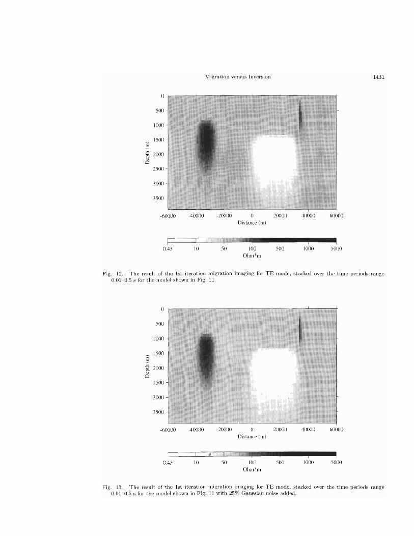
Figure 11 shows a mod el with one resistive (5000 Ohm-m ) prism atic insertion , and one conduct ive (0.5 Ohm-m) within a 250 Ohm-rn background . The syntheti c "observed field" components were ca lculate d using th e sa me P\V2D forward modeling code . The N = 121 observat ion points X i (i = 1,2 , .. . , N ) were located along the profile on th e eart h 's surface with the separation b.x = 1000 m. We have computed the elect ric: Ey and magneti c: H 2: fields for the periods 0.010.25 s. As we can see in Fig. 12, l st itera tion migration allows us to resolve both t he resistive and th e conduct ive objects. vVe have t he sa me result even if we add 25% Gaussian noise to t he observed data (Fig. 13).

So far , we have discussed results of applying migration imaging to 2-D mod els in TE mod e. However, we can re pea t for TM mod e as well all the derivations mad e above for TE mode. We thus obt ain th e following imaging condit ions for TM mod e data:

b.O"ma (x , z) = koRe 1H~ (:1: , z) H;-m (:1:, z) dio, (42) n

Thus, we can see that th e migration anomalous conduct ivity for TM mode is equal to t he integral over frequencies of the product of t he incident (background) magneti c field Ht and the migrated residual magneti c field H; TTl. Figure 14 presents t he 1st iteration migration results for TM mode data , calc ula ted for t he same mod el shown in Fig. 11. \Ve can sec that the migration image for T M mode is exact ly the same as for T E mode (Fig. 12).

We have also applied RRI method to inverse TE and TM dat a for the same model. The resul t s of inversion are shown in Figs. 15 and 16. T hese images are compat ible with those obtained

o I I!

500

1000

1500 E :5Co

2000 u

::::l

2500

3000

3500

-60000 -40000 -20()OO o 20000 40000 60000 Distance ( Ill)

1.0 10 50 100 500 1000 5000 Ohm*m

F ig. 11. 2-D resis tiv ity mod el wit h o ne resistive (5000 O hrn -rn ) prism atic insert ion , a nd one conductive (0.5 Ohrn-m) wit hin a 2.';0 O hm-rn back gr o und .


0

SOO

1000

ISOO

E t 2000

~"2500

3000

3S00

-60000 -40000 -20000 0 20()OO 40000 60000 Distance (m)

O,4S 10 SO 100 50() 1000 SOOO Oh III *III

F ig. 12. The res ult of the l st it erati on m igrati on im aging for T E mo d e , stacked over the t ime per iods range 0.01 -0.5 s for t he mod e l s how n in F ig. 11.

0

SOO

lOOO

ISOO

~

~ 2000

CI"2500

300 0

3S00 .. -60000 -40000 -20000 o 40000 60000

Distance (Ill)

20000

0,4 5 10 50 100 SOO 1000 SOOO Ohm *1l1

Fig . 13. The result. of t he l s t iterat ion mi gr at ion im agin g for T E mod e . stacked ove r the t ime peri od s ran ge 0 .01 -0.5 S for t he model s how n in Fi g. 11 wit h 25'7c Gaussian noise added .

1432 M. S. Z lIDANOV a nd P. T R.AY!'I:"

o I..... . .. • Of. lot. . • j

500 ·

1000

~ 1500 g E. 2000 <lJ

c 2500 ·

3000 ·

3500 ·

-60000 -40000 -20000 0 20000 40000 60000 Distance ( Ill)

• II I i 0.45 10 50 100 500 1000 5000

Oh111 *III

Fi g. 14. The res ult of t he 1st iterat ion migra t ion imaging for T N! mod e, stacked over t he ti me periods range 0.0 1- 0.5 s for t he same mod el shown in Fig. 11.

o I I

1000

2000 ·

3000

4000 -60000 -40000 -20000 0 20000 40000 60000

I I I I I i i 0 34 67 100 134 167 200

log(Ohm*m)

F ig. 15. The inverse mo del obt ained for the model shown in F ig. II usi ng Ra pid Relaxa tion Invers ion (R R I) code by Booker and Smit h (1991) for TE mode afte r 35 it era tion s.

1433 Migr ation versus In ver sion

o · 11=~__:-'-__--'- ...l......~_--..-.l~__....l....__--+

1000

2000

3000

4000 -60000 -40000 -20000 0 20000 40000 60000

,

i e ••II I I I I i 0 34 67 100 134 167 200

(Ohm*m)

Fig. 16. The inv erse model ob t ained for the mod el shown in F ig, 11 us ing Rapid Relaxa ti on Inv er sion (RR I) code by Booker and Smit h (199 1) for 'I' M mod e after :~5 ite ra t ions .

by migration. They produce better estimat ion of the depth of the resistive body. Meanwhile, the CPU time for run is ab ou t 35 Min for 1'E mod e and 29 Min for 1'1.1 mode, while in t he case of migration it too k only 23 s to act ually generate the image.

6. Conclusion

The resul ts of t heoretical ana lysis present ed in this pap er demonst rate that there is a very close connec t ion between th e method of E i'vl migration , developed in our ea rlier pap ers, and the solut ion of th e convent ional EM inverse problem. Actually, we can say now that migration is an approximate inversion. It realizes the first it eration in th e inversion algorit hm, based on the minimization of th e residual field energy flow through the profile of observations. This new theoretical result suggests a new imaging condition formul ation and indicat es a new approach to EM imaging , based on it erative migration. The iterative migra tion form s a prin cipally new method of interpreting EM data , which combines t he ideas of downward cont inuat ion and traditional inver sion . Numerical modeling demonstrates that migration generates reasonable images of the subs urface st ructures an order faster than rigorous inversion .

We also should notice in t ho conclusion th at there are some lim itations in using migration for interpretation of E~vl data . T he main problem is t hat the background cond uct ivity distribution used for migra tion should be known a pr iori, while in the case of convent iona l inversion it is usually genera ted in t he process of inverse problem solution. Different ways of solving this problem have been discussed in our paper (Zhdanov et 0,[ ., 1996).

Another problem is relat ed to the fact that the migration is based on the tran sformation of th e electric and magneti c fields observed on th e sur face of the eart h, and cannot handle the imp edances, which are usu ally record ed in t he case of magnet ot elluric observat ions. P ractical ap


plication of the migration would require implementation of a special observation system designed to obtain the synchronous distribution of electromagnetic field along the profiles on the earth's surface. It can be done by simultaneously using one moving observation and one fixed reference station and by applying transfer function technique to process these data. One can find more details about this technique in the book by Berdichevsky and Zhdanov (1984).

Financial support for this work was provided by the National Science Foundation under grant No. EAR-9403925.

We also thank the University of Utah Consortium of Electromagnetic Modeling and Inversion (CEMI), which includes CRA Exploration Ltd., Mindeco, MIM Exploration, Naval Research Laboratory, Newmont Exploration, Western Mining, Kennecott Exploration, Schlumberger-Doll Research, Shell International Exploration and Production, Western Atlas, Western Mining, the United States Geological Survey, Unocal Geothermal Corporation, and Zonge Engineering for providing additional support for this work.

We are thankful to the reviewers, Drs. C. Farquharson and D. Avdeev, for their helpful remarks.

Appendix A: Calculation of the First Variation of Electromagnetic Field

Perturbing Eq. (1) we obtain the equation for the first variation of the electric field:

n 2 "E . "E _ { -iw/-LobO"Ey, (x, z) E D (A.l)v u y +~w/-LoO"u y - 0, (x,z) ~ D

We now introduce the Green's function G er of the geoelectrical model with the conductivity 0" = O"(x,z). The Green's function depends on the position of the points (x,z) and (x',z') and is determined by the equation:

V 2G er (x, z lx', z') + iW/-LoO"Ger (x, z lx', z') = -b (x - x', z - z') , (A.2)

where 8 (x - x', z - z') is two-dimensional Dirac function. According to the Green's formula:

j, (abE yG - aG erst:y) dl = if (G V 28E - si:yV2G a ) ds (A.3)a a a y ,

L an n s

where n is the direction of the outer normal to L. Let us assume now that the region 8 is a big circle with the center inside domain D and of

radius R which is so big that D C 8. Taking into account Eqs. (A.l) and (A.2) the Eq. (A.3) can be rewritten as:

[ (iJ~:y c, - (:~: bEy) dl = fl (-iWlloGubuEy HEyb (x - x', z - z')) ds. (AA)

Let us expand the radius R of the circle L to infinity. Then the curvilinear integral will go to zero, because, due to the radiation conditions, functions bEy and Ger vanish rapidly at infinity, and we finally obtain:

bEy (x', z') = iW/-Lo fj~ Ger (:r - x', z - z') . bo (x, z) Ey (x, z) ds. (A.S)

The first variation of the magnetic field bHx can be calculated from bEy using Maxwell's equations:

" 1 abEy (x', z') if aG er (x - x', z - z')bHx(x,z)=--.- a' =- a' /jO"(x,z)Ey(x,z)ds, (A.6)

~W/-Lo z D z

where domain of integration changes from 8 to D because of Eq. (14).


Appendix B: Integral Representations for Electromagnetic Migration Field

Following our previous publications (Zhdanov and Keller, 1994; Zhdanov et al., 1996), we introduce the EM migration field as the solution of the boundary value problem for the adjoint Maxwell's equation. In the case of E-polarization and in the frequency domain, the E:;* component of the EM migration field satisfies the equation:

\72E ym* - iWIJt"'0 (JEY

m* = ° ,-z > ° (B.1)

everywhere in the lower half-plane, vanishes according to the radiation conditions at the infinity, and is equal to the observed field on the surface of observation z' = 0:

E:;* (x',z = O,w) = Ey (x',z = O,w),

(B.2)oE:;* (x', z', w) I = oEy (x', z', w) I ;:, , ;:, , ' uZ z'=O uZ z'=O

where asterisk * denotes complex conjugate values. We have the same conditions for the migrated residual field E~:

n2v E/).m* - iWIJt"'0 (JE/).m* ,_ Z > ° y Y = ° (B.3)

and

E;-m* (x',o,w) = E;- (x',o,w)

oE;-m* (x', z', w) I oE~ (x', z', w) I oz' oz'

z'=O z'=O

The complex conjugated Green's function C~b satisfies the following equation in the lower half-plane:

\72C;b (x, z [z', z') - iW/-LO(JC;b (x, z lx', z') = -/5 (x - x', z - z') . (B.4)

We can now apply Green's formula taking into account Eqs. (B.3) and (B.4) and repeating the derivations similar to the one described in Appendix A. As the result, we find the expression for the migrated residual electric field as an integral over the profile of observations, horizontal axis x, of the residual electric field:

+ CXl ( oE/). (x' z') nc: (x z lx' Z'))J C * ( I" ) y , - E/). (' ') , d ' o i, x, Z X , Z Bz' y x, z O"b'oz' x

-CXl z'=O = E~m* (x, z) . (B.5)

Taking complex conjugated values of the left-hand and right-hand parts of Eq. (B.5) we determine:

+ CXl ( oE/).* (x' z') ec ( I"))J " ) y , - E/).* (' ') O"b x, Z X , z d'C a i, (x, Z IX , Z ;:, , y x, z ;:, , x -CXl uZ uZ

= E~m (x, z) . (B.6)

The last two equations give the integral representations for the solution of the boundary value problem for the migrated residual field.

Appendix C: Definition of the Length of the Step ko

The optimal length of the step ko can be determined by minimization of the functional [O"b (x, z) - kol (x, z)] = (ko).

We denote by E~l), H~l) the EM field components corresponding to the geoelectrical model

with the conductivity distribution 0" = O"b (x, z) - kol (x, z). Let us substitute E~l), H~l) into Eq. (12) ,

 = ~ j'1+ 00

(E(l)6. H(l)6.* + E(l)6.* H(l)6.) dx'dw (C.1)4 y x y x , 12 -00

where E(l)6. = Eobs _ E(l) H(l)6. = Hobs - H(l) and the calculation of theoretical field E(l)y y y, x x x, y,

H~l) is linearized, using Born approximation (Berdichevsky and Zhdanov, 1984):

E~l) = E~l) (x', 0, w) ~ Et (x', 0, w) + iW/-Lo / Is CUb (x - x', z) DO" (x, z) Et (x, z) ds

Et (x',o,w) - koEt (x',o,w) , (C.2)

H~') = H~') (x', 0, w) '" H~ (x', 0, w) - / Is DCa, (x ~z~" z - z') I,'~o DO" (x, z) Et (x, z) ds

H~ (x',o,w) - koH~ (x',o,w), (C.3)

where DO" (x, z) = -kol(x, z) and Et, H~ are the fields, calculated using Born approximation for the model, perturbed in the gradient direction:

Et (x', 0, w) = iW/-Lo / Is CUb (x - x', z) l (x, z) Et (x, z) ds, (C.4)

I 1 oEtH =--- (C.5)

x iW/-Lo oz' .

Substituting Eqs. (C.2) and (C.3) into Eq. (C.1), we obtain:

00

~ 11+ (E(1)6.H(l)6.* + E(1)6.* H(l)6.) dx'd = 4 y x y x W 12 -00

~ 1,1:= {[E; HoE;] [H;' +koH;]'

+ [E~ + koEtJ * [H~ + koH~J } dx'dw. (C.6)

Now we can find the first variation of (ko) with respect to ko:

00

D. (k ) = ~Dk 11+ { [E 1H6.* + E6.H 1* + E 1*H6. + E6.*H1JkO 0 4 0 y x y x y x y x 12 -00

+2ko [EtH~* + E;* H~J } dx'dw. (C.7)

After some algebraic transformations, we obtain:

DkO (ko) = ~Dko { F" {Re [EtH~* + E~ H~*J + 2koRe [EtH~*J } dx'dw. (C.8)2 J12J- oo

The necessary condition for minimizing (ko) is:

6ko (ko) = O.

Therefore, we have:

l i:= {Rc [Et H;" + E~ H~'] + 2koRe [EtH~:]} dx'dw = 0

From the last equation we find at once:

Re r r: [El H6.* + E6.HI*] dx'dwIn -00 Y x Y xko (c.g)

2Re r J+oo El Hl*dx'dw In -00 Y x

REFERENCES

Berdichevsky, M. N. and M. S. Zhdanov, Advanced Theory of Deep Geomagnetic Sounding, 408 pp., Elsevier, Amsterdam, 1984.

Pankratov, O. V., D. B. Avdeev, and A. V. Kuvshinov, Scattering of electromagnetic field in inhomogeneous earth. Forward problem solution, Fizika Zemli, No.3, 17-25, 1995.

Smith, J. T. and J. R. Booker, Rapid inversion of two- and three-dimensional magnetotelluric data, J. Geophys. Res., 96, 3905-3922, 1991.

Stratton, J. A., Electromagnetic Theory, 615 pp., McGraw-Hill Book Company, New-York and London, 1941. Tarantola, A., Inverse Problem Theory, 613 pp., Springer-Verlag, Berlin, Heidelberg, New York, 1987. Wannamaker, P. E., J. A. Stodt, and L. Rijo, A stable finite element solution for two-dimensional magnetotelluric

modeling, Geoph. J. Roy. Astr. Soc., 88, 277-296, 1987. Zhdanov, M. S., Tutorial: Regularization in inversion theory, Colorado School of Mines, 1993. Zhdanov, M. S. and G. V. Keller, The Electromagnetic Methods in Geophysical Exploration, 873 pp., Elsevier,

Amsterdam, 1994. Zhdanov, M. S. and O. Portniaguine, Time domain electromagnetic migration in the solution of the inverse

problems, Geophys. J. Int., 1997 (in press). Zhdanov, M. S., P. Traynin, and O. Portniaguine, Resistivity imaging by time domain electromagnetic migration,

Explor. Geophys., 26, 186-194, 1995. Zhdanov, NI. S., P. Traynin, and J. Booker, Underground imaging by frequency domain electromagnetic migration,

Geophysics, 61, 3, 1996.

migration versus inversion in electromagnetic imaging

Documents