milgrom and roberts, “risk sharing and incentive contracts,”

RISK SHARING AND INCENTIVE CONTRACTS

ell, then, says 1, what's the use you learning to do right when it's troublesome to do right and ain't no trouble to do wrong, and the wages is just the same?

Huckleberry Finn'

In Chapter 6, we examined how insurance of various forms can combine with difficulties of monitoring actions or verifying information to blunt individual incentives. We also surveyed a number of responses to such moral hazard problems. Among these were incentive contracts, under which individual incentives are strengthened by holding people at least partially responsible for the results of their actions, even though doing so exposes them to risks that could be more easily borne by an insurance company. In this chapter, we develop a detailed theory of the nature and form of efficient incentive contracts in the presence of moral hazard, establishing a number of general principles that can be used to understand, evaluate, and design such contracts. Although we develop this theory largely in terms of employment contracting and performance pay, the principles are broadly applicable to a wide variety of institutional contexts.

INCENTIVE CONTRACTS AS A RESPONSE TO MORAL HAZARD

In both theory and practice, there are more options open to society than to insure a risk fully or not to insure it at all. Actual insurance contracts are also incentive

206 1 The Adventures of Huckleberry Finn, Mark Twain (1884).

207

contracts: They have provisions that restrict and condition claim payments in ways that provide better incentives than full insurance without removing the essential part of the insurance coverage. The deductible clause that is common in homeowners' fire and theft insurance policies requires the policyholders to bear the initial part of any loss they may incur while still protecting them against large financial losses. Health-insurance policies often require copayments, according to which the insurance pays only a fraction of the costs, with the rest being borne by the insured. Automobile insurance is experience rated, so that those who are responsible for traffic accidents pay higher rates. These features are designed to encourage the insureds to take care and to deter their excessive use of the insurance. For example, the copayments on emergency room visits are set so that, rather than automatically rushing to the emergency room, a patient will wait to be treated in the doctor's office for illnesses and injuries that are not extremely urgent. In this spirit, the policy may provide no coverage at all for treatments that are considered to be elective, such as cosmetic surgery other than that which is necessary to repair damage caused by an injury. As these examples make clear, insurance contracts are designed with profound attention for the need to reduce the waste caused by moral hazard.

Similar moral hazard issues must be faced when devising compensation contracts for employees in a firm. Here, too, there is a balance that needs to be struck between providing incentives and insulating people from risk. To provide incentives, it is desirable to hold employees responsible for their performance; this means that employees' compensation or future promotions should depend on how well they perform their assigned tasks. As we will see, however, holding employees responsible typically will involve subjecting them to risk in their current or future incomes. Because most people dislike bearing such risks and are often less well equipped to do so than are their employers, there is a cost in providing incentives. Efficient contracts balance the costs of risk bearing against the incentive gains that result.

Sources of Randomness If employees were always able to perform as required and if it were easy to determine precisely whether they have behaved as they were supposed to, having pay depend on performance would not generate any risk-bearing costs. An employee could choose whether to perform appropriately or not. Appropriate behavior would be compensated as agreed; inappropriate behavior would go uncompensated and might be penalized. Higher levels of required performance would be associated with higher pay to compensate for the additional effort that the employee is called upon to expend, but there would be no risk in the employee's pay because the outcome is completely under the employee's control.

In most real situations, however, attempts to impose responsibility on employees for their performance do expose them to risk because perfect measures of behavior are hardly ever available. For example, if the employee is expected to give expert advice on some matter, it may be impossible to determine whether the advice is based on the best available information and analysis and whether the recommendations are actually designed to promote the employer's interests, or whether the employee has acted selfishly or deceptively. When care and effort are wanted, it may equally be impossible to determine if employees are doing what they should or slacking off. In these kinds of situations, even though the quality of effort or the accuracy of information cannot itself be observed, something about it can frequently be inferred from observed results, and compensation based on results can be an effective way to provide incentives. Piece rates are a prime example: Rather than trying to monitor directly the effort that the employee provides, the employer simply pays for output.

However, results are frequently affected by things outside the employee's control

Risk Sharing and Incentive Contracts

208

Efficient that have nothing to do with how intelligently, honestly, and diligently the employee

incentive& has worked. Sales at a fast-food restaurant may be lower than expected due to the outlet

Contracts and manager's lack of creativity in devising promotional efforts or negligence in supervising Ownership the staff, but the low level may also be caused by other factors. Road construction could

have made the location less accessible to customers. The opening of a competing restaurant nearby could be to blame. Population growth may have been less than forecast. In the case of a franchise, the franchisor's failure to provide attractive menus or timely deliveries of food could be responsible. Or some combination of these and other factors might be at work. Similarly, if an aircraft crashes, pilot error may be to blame, or poor maintenance, or a design flaw in the craft itself, or a bolt of lightning, or an air traffic control error, and so on. When rewards are based on results, uncontrollable randomness in outcomes induces randomness in the employees' incomes.

A second source of randomness arises when the performance itself (rather than the result) is measured, but the performance evaluation measures include random or subjective elements. For example, the way an employee is evaluated may depend on his or her supervisor's subjective perception of the employee's attitude towards the job and behavior towards other workers. Employees may see this sort of evaluation as a source of risk because it is based partly on elements outside the employee's control. A worker's performance may be evaluated by sporadic monitoring, and these random observations may not give a perfect reflection of the actual quality of the work. In either case, the imperfect evaluation of performance induces randomness in rewards.

A third source of randomness comes from the possibility that outside events beyond the control of the employee may affect his or her ability to perform as contracted. Health problems may reduce the employee's strength and ability to work, concerns about family finances may make it impossible to concentrate effectively on the tasks at hand, or weather or traffic conditions may render meeting a regular schedule impossible. Thus, performance itself becomes random, and so too does performance-based compensation. Consequently, making employees responsible for performance subjects them to risk.

Balancing Risks and Incentives

It might be possible to insulate employees from these risks by making their compensation absolutely risk free and unrelated to performance or outcomes. In that case, however, the employees would have little direct incentive to perform in more than the most perfunctory fashion, because there are no rewards for good behavior or punishments for bad. As we will see, both here and in Chapter 12 (where we examine compensation issues more specifically) effective contracts balance the gains from providing incentives against the costs of forcing employees to bear risk.

The same considerations arise in many other business transactions. The size of the crop produced by a sharecropper is influenced by weather and pests as well as by the sharecropper's own skill and effort. Traditionally, landowners make part of the sharecropper's compensation proportional to the size of the crop. This arrangement provides helpful incentives that induce the sharecropper to plant drought- and pest-resistant varieties, to irrigate and care for the crops, and so on. However, it also exposes the sharecropper to the risks of a poor harvest—a risk that is at least partially outside his or her control. Similarly, in the United States, a lawyer who sues for damages on behalf of a client often receives a contingency fee (a percentage of the damage award or settlement). This system provides the litigator with an incentive to work hard on behalf of the client, but because the outcome of the lawsuit is not entirely under the litigator's control, both the litigator's income and the client's arc uncertain.

Although all of these cases share certain common features, the accuracy of the performance assessments that can be achieved and the need for and possibility of risk

209 sharing or insurance vary from case to case. Because of these differences, the Risk Sharing and institutions and practices that best balance risk and incentives also vary. Incentive Contracts

The conclusion that arrangements should vary from case to case is too vague to be of any use to managers or interest to economists. Fortunately, we can do better. The principles developed in this chapter make it possible to reach a relatively subtle understanding of how optimal practices can be designed that trade off the value of protecting people from risk against the need to provide them with incentives.

In order to analyze how rational people respond to incentives in insurance-like contracts, we must first examine how rational people behave and interact in risky situations. This involves three steps. The first is to describe the risks precisely, using the language of statistics. Then, we describe how rational people, acting individually, can choose consistently among risky choices and how varying individual attitudes toward risk taking can be incorporated into the analysis. Finally, we examine how groups of people can share risks and form insurance pools, being careful to quantify the benefits of insurance coverage. Given this background, we then examine how people respond to incentives in risky situations. This then allows us to develop the principles of efficiently designed incentive contracts.

DECISIONS UNDER UNCERTAINTY AND THE EVALUATION OF FINANCIAL RISKS

The first element we need is a theory of decisions under uncertainty. There are, in fact, a number of rich theories addressing this subject in great generality, but for our purposes it is enough to consider the special case in which the risks are financial. The first step is to describe the financial risk. We do this using two ideas familiar from statistical theory: the concepts of mean and variance. These terms are defined in the appendix to the chapter. Here, we illustrate their meaning by computing the mean and variance in an example.

Computing Means and Variances

Recall that the mean or expected value of a random income is simply the expected amount of income, computed as the weighted average of the possible values that income might take on, with the weight on each value being the probability of that value occurring. The relevant calculations are illustrated in Table 7.1.

The table shows a hypothetical situation in which there is an investment for which the returns are zero with probability one half, $3,000 with probability one third and $6,000 with probability one sixth. The mean or expected value of the return is 4($0) + ($3,000) + i($6,000) = $0 + $1,000 + $1,000 = $2,000. In the table, the calculation works by multiplying the entries in columns 1 and 2 to obtain column 3, and then summing the column. Having higher probabilities on higher values increases the mean.

The variance of income is a measure of its variability or randomness. It is computed in columns 4 and 5 of the table. In column 4, we take each possible value, subtract the mean (to get a measure of how far the particular value deviates from the expected value), and square the result (so that terms greater than the average that result from higher-than-expected incomes do not cancel out the negative terms that result when income is less than expected). In column 5, these squared variations are multiplied by the corresponding probability. Summing the column gives the variance. In the example, the variance is 4(0 — 2,000) 2 + (3,000 — 2,000)2 + i(6,000 — 2,000)2 = 4(4,000,000) + 4(1,000,000) + (16,000,000) = 5,000,000. (The units are "dollars squared.") If income is certain, then the variance is zero, because the income never deviates from its expected value. Increasing the probability of very high and very low values tends to increase the variance.

210 Table 7.1 Sample Computation of Mean and Variance Efficient

Incentives: Contracts and

Ownership 1 2 3 4 5 Probability Return (I) x (2) (Return — Mean)2 (1) x (4)

1/2 0 0 4,000,000 2,000,000 1/3 3,000 1,000 1,000,000 333,333 1/6 6,000 1,000 16,000,000 2,666,667

Mean 2,000 Variance = 5,000,000

Certainty Equivalents and Risk Premia

One of the main hypotheses we employ in this chapter is that most people are risk averse-, that is, they would prefer receiving a certain income of T to receiving a random income with expected value T. The amount the person would be willing to pay to make the switch is the risk premium associated with the random income. The magnitude of the risk premium depends on both the riskiness of the income and the individual person's degree of risk aversion. The amount that is left after the risk premium is paid is the certainty equivalent of the random income. It is the amount of income, payable for certain, that the person regards as equivalent in value to the original, random income.

One of the central results of decision theory is that the certainty equivalent can be estimated by a simple formula: T - ir(T)Var(I), where I and Var(I) are the mean and variance of the random variable I, and r(T) is a parameter of the decision maker's personal preferences called the coefficient of absolute risk aversion for gambles with mean T. The mean in this formula is the mean income, and the amount subtracted from it in the formula is the risk premium; it is equal to one-half times the coefficient of absolute risk aversion times the variance of the income. According to the formula, the risk premium is proportional to the coefficient of absolute risk aversion: People who are more risk averse according to this measure are willing to pay proportionately larger risk premiums to avoid a given risk. If the coefficient of absolute risk aversion is zero, then the person is unwilling to pay any premium to avoid the risk. Such a person is called risk neutral. A person is risk averse when the coefficient of absolute risk aversion is positive. The amount I — 4r(l )Var(1) that is left in expectation after the risk premium is deducted is called the person's certain equivalent income or the certainty equivalent of the random income I.

If there is no uncertainty regarding the level of income, then Var(I) = 0; the only value that income actually might take on is / = T. Then, the formula yields the sensible result that the person is as well off with the nonrandom income 1 as with a certain amount that is equal to I: The thing is as pod as itself. When I does vary (so Var(1) is positive) and the person is risk averse (so r(I)is also positive), the risk premium is positive. This means that he or she would be willing to accept a lower amount than T to avoid the risk. More precisely, the risk premium, ir(T)Var(I), is the amount that the person would pay to have the certain income 1 for sure rather than face the uncertainty in 1. 2

The estimate of the certainty equivalent given in this formula is good when the variance is not too large or the coefficient of risk aversion is small. In terms of the example in Table 7.1, where the mean income was $2,000 and the variance was 5,000,000, the formula becomes 2,000 — 2,500,0004). This approximation is reasonable only for values of r in the range of .00008 or less (corresponding to a risk premium of 200); when r .0008, it yields the nonsensical answer that the individual would be indifferent

211

Risk Premia and Value Maximization

Our analysis in this chapter uses the value maximization principle, which in the context of uncertainty asserts that an arrangement is efficient if and only if it maximizes the total certain equivalent wealth of all the parties involved. Recall from Chapter 2 that the premises needed to derive the principle are (1) that each person has enough wealth to make whatever payments might be called for under any relevant contract and (2) that each person has a well-defined willingness to pay for any given product or service and the amount of this monetary valuation does not depend on his or her income level. As discussed in Chapter 2, these are strong and often unrealistic assumptions, but they greatly simplify the analysis and enable us to separate analytically the effects of the level and variability of income from all other effects on the matters of interest. In the context of uncertain income, the second assumption is reduced to this: The risk premium that a person would pay to eliminate a given amount of variance must not depend on the expected level of income I. In view of the risk premium formula, this means that r(I) must not depend on I. Throu&hout the rest of this chapter, we make that assumption and write r instead of r(I). With this assumption, the crucial formulas become:

Expected Income = Risk Premium = frVar(1)

Certain Equivalent = 1 — frVar(I)

We use these formulas to calculate the benefits of insurance and the costs of the risk bearing that is required to provide incentives.

RISK SHARING AND INSURANCE

One of the most fundamental facts about the economics of risk is that when several people are facing statistically independent risks, then by sharing the risks among themselves they can greatly reduce the cost of risk bearing. Two risks are statistically independent if knowing the realized value of one risk gives you no information about the value that the other will achieve. For example, the amount you won or lost per dollar invested in the state lottery today does not give you any reason to change your estimates of the likely returns in the stock market tomorrow. In contrast, for risks that are not independent, knowledge of one is useful in predicting the other. For example, the prices of gold on the London and New York markets are both random, but they tend to move together under the influence of arbitrage (buying in one market and selling in another to make a riskless profit). Thus, knowing the price in London tells you something useful about what the New York price is likely to be, and so the two risks are not independent. This principle of risk sharing—that sharing independent risks reduces the aggregate cost of bearing them—is the basis of all financial insurance contracts.

How Insurance Reduces the Cost of Bearing Risk

In modern economies there are many kinds of institutions to assist people in sharing risks. One important group consists of the insurance companies. Having many policyholders, the insurance companies can spread risks very widely, enabling the companies to reduce individual risks greatly. If the risks are independent and the number of policyholders quite large, the risks are effectively eliminated and insurance works very well. For example, the risk that you will suffer an automobile accident is

between the gamble and getting a negative income for sure. In using the approximation, we thus assume that the variance of the uncertain income is not too large relative to the individual's risk aversion.


212 Efficient very nearly independent of the risk that any other particular person will do so, therefore

Incentive= automobile insurance is a feasible enterprise. Insurance companies specialize in Contracts and evaluating individual risks and, by pooling the risk-bearing capacity of policyholders

Ownership and (sometimes) shareholders, they reduce the cost of the risk bearing to negligible proportions. Pooling independent risks also has the additional advantage of making the insured losses statistically predictable. An insurance company can ask each insurance policyholder to pay a price for insurance equal to the expected amount of the loss, plus a margin for expenses and profit, and can be reasonably sure that the aggregate premium income together with a proportionately small reserve fund will enable it to pay for whatever losses may be suffered, even in a bad year.

Some kinds of risks, however, are so large and pervasive in their impact that they cannot be made negligible by sharing and they cannot be managed by traditional insurance arrangements. (Technically, the risks that people bear in this case are not statistically independent.) For example, an oil price increase would have such widespread effects, reducing the effective incomes of most people in oil-consuming countries, that no amount of risk sharing among those oil consumers can insulate them from the loss. Risks of this general kind are shared through other markets, especially the financial markets. By purchasing stock in companies that own oil reserves, for example, an investor who is especially vulnerable to oil price increases can arrange to have an offsetting profit if oil prices increase. Financial markets allocate many other kinds of risks, as well. For our purposes, an important example is the investment risks that are taken by firms, such as those associated with a new technology. The risk of failure of the technology is borne by shareholders in the company that develops it, and this capacity for risk sharing reduces the firm's cost of financing the investment, helping to promote technical change.

Efficient Risk Sharing: A Mathematical Example

Suppose that there are two people, A and B, each of whom has some risk associated with his or her income, where these risks are independent. Let and I. represent their random incomes, with means I A and 19 and variances Var(1 A ) and Var(1 a ), and let rA and r. denote their coefficients of absolute risk aversion. In view of our earlier assumption, the value maximization principle applies. Consequently, every efficient risk-sharing contract maximizes the total certain equivalent income of all the parties, and every such contract is an efficient one.

If the parties make no special arrangements, then the total cost they suffer on account of risk bearing, that is, the total risk premium, is ir AVar(IA) + which is the sum of the two individual risk premia. Suppose that the parties instead agree on a risk-sharing contract with party A receiving a fraction a of the income IA and B of the income i (and thus of the risks associated with the two uncertain incomes.) In addition, suppose A receives a cash transfer of -y for the risk-sharing services provided. (This transfer might be positive or negative, but it is independent of the actual, realized incomes.) Party B receives the remaining share of each risk and makes the cash payment -y. After this agreement, A's income will be ct1 A + B19 + and B's will be (1 — a)IA + (1 — B)19 — y. This is a feasible agreement because the total income each party receives always adds up to IA + 1, the amount available. With this agreement, the total risk premium of the two parties is:

Total Risk Premium = 4rAVar(tx1A + B/. + -y) + fr.Var((I — a)1A + (1 — 13)1 9 — (7.1)

Because the total certain equivalent income of the two parties is equal to the mean income, IA + I., minus the risk premium, the efficient arrangements are those that minimize Equation 7.1.

213

Using identities about variances (see Formula 7.18 in the appendix), Equation Risk Sharing and

7.1 is a quadratic function of a and B. The total risk premium is minimized when Incentive Contracts a./(1 — a) =- B1(1 — B) = TB/TA . For example, suppose rA = 2 and r5 = 4. The higher value for B's coefficient of absolute risk aversion indicates that B finds bearing risk more onerous than does A. Indeed, the risk premium that B attaches to any given risk is twice the amount A would pay to avoid the risk. In these circumstances, we might expect that A would bear more of the risk than would B. Evaluating the solution, we see that «1(1 — a) = — 13) = 2, so a = B = and (1 — a) = (1 — B) = I: A does in fact bear most of both risks. Moreover, A bears the same share (two thirds) of both.

To formulate the general principle that applies here, it is helpful to think in terms of different peoples' capacity to bear risk. We measure this by introducing the notion of risk tolerance. Someone with a coefficient of absolute risk aversion of r will be said to have risk tolerance of 1/r. Notice that in the preceding example, A's share of each risk is equal to A's share of the total risk tolerance = 41(1 + 1)).

These calculations actually reflect a general principle that can be shown to hold for any number of people and any number of financial risks: When risks are shared efficiently, the share that a party bears in each risk is the same and is equal to his or her share of the total risk tolerance of the group. Moreover, when risks are allocated efficiently, the total risk premium comes out to be:

Total Risk Premium = 1 Var(IA + IB)4R1/TA) ( 1 /r8)] (7.2)

Equation 7.2 resembles the formula for the risk premium charged by a single decision maker. It says that when risks are shared efficiently among a group of people, the total risk premium is the same as if the total risk were borne by a single decision maker whose risk tolerance is the sum of the members' individual risk tolerances. In the preceding numerical example, (1/r A)+(l/r0) 4 + L This formula, too, is general; it can be shown to hold for any number of people and any number of financial risks. With efficient risk sharing, the group is less risk averse than the people comprising it and so the costs of bearing risks can be reduced.

When individual risks are independent, these facts imply that sharing risks can be a very effective way to reduce the cost of risk bearing. For example, if there are n people, each with an income with variance v and each with the same coefficient of risk aversion r, and if each bears the income risk separately, then the risk premium will be try per person. If the people share the income risks efficiently, then each will have a 1/n share of the total risk. The variance of the total risk is V -= nv, so the variance of an individual 1/n share is Vitt' = yin (see Formula 7.18 in the appendix again). Therefore, by sharing risks, each person's risk premium is reduced from irv to Irvin. When n is large, even substantial financial losses can be reduced to economic insignificance by sharing them efficiently across the group.

Optimal Risk Sharing Ignoring Incentives For both insurance companies, with their wide base of policyholders, and publicly traded corporations, with their wide base of shareholders, it is reasonable to suppose as a first approximation that the total risk tolerance of the company is infinitely larger than the risk tolerance of any individual policyholder or employee. As we mentioned earlier, an institution or person with infinite risk tolerance is said to be risk neutral: The coefficient of absolute risk aversion is zero and so the risk premium for bearing any risk is also zero. Applying our general propositions to the case where risks are to be shared between a risk-neutral insurance company and a risk-averse insurance policyholder or between a large, risk-neutral employer and a risk-averse employee, we find that the optimal share of the risk to be borne by the insurance buyer or employee

214

cient is zero. Efficient risk sharing requires shifting all the risk onto the risk-neutral party, Effi

Incentives: who suffers no cost in bearing the risk. Contracts and This conclusion, however, depends on ignoring the incentive problems for

Ownership insurance and employment created by the condition of moral hazard.

PRINCIPLES OF INCENTIVE PAY

The general problem of motivating one person or organization to act on behalf of another is known among economists as the principal-agent problem. This problem encompasses not only the design of incentive pay but also issues in job design and the design of institutions to gather information, protect investments, allocate decision and ownership rights, and so on. However, we focus our discussion in this chapter principally on the issues surrounding incentive pay, and we set our discussion of incentives in the context of employment. The principal in this case is the employer, who wants the employee (the agent) to act on his or her behalf.

Basing Pay on Measured Performance

As we discussed in the introduction to this chapter, there are many situations in which providing incentives requires that employees' pay depend on their performance. Essentially, if the employees' direct provision of effort, intelligence, honesty, and imagination cannot be easily measured, then pay cannot be based on these and any financial incentives must come from basing compensation on performance. Efficient risk sharing, in contrast, requires that each person in society should bear only a tiny share of each risk, without regard to its source. In particular, individuals should be insulated against the randomness that would enter their pay by basing it on measured performance. Therefore, performance-based compensation systems cause a loss from inefficient risk sharing. The money value of the loss is equal to the risk premium associated with the actual compensation system minus the risk premium that would be associated with efficient risk sharing. Firms that use performance-based compensation hope to recoup this loss (and more) by eliciting better performance from their employees.

There are various reasons why incentives might be needed to elicit top-notch performance. Some employees may find their work distasteful and may neglect it unless they are held responsible for achieving results. Even when employees are hard workers who like their jobs, they may still have priorities that are different from those of their employer. For example, without compensating incentives, managers might be tempted to be too generous to their subordinates in granting raises and time off, or to hire the children of relatives and friends, to spend lavishly on a pleasant work environment or on fancy accommodations when traveling on business, to use company resources for community projects that raise their personal status, to devote excessive efforts to projects that advance their careers or that are especially interesting or pleasant, and so on.

To analyze these possibilities in a model, we suppose that the employee must exert an effort e at personal cost C(e) to serve the interests of the employer. The effort e represents any activity that the employee undertakes on behalf of the firm, and the cost C(e) can represent the unpleasantness of the task, foregone perquisites, lost status in the community, or anything else that the employee gives up to serve the employer's interests. For tasks that are pleasant, the "cost" can be zero or even negative.

The effort e is assumed to determine to the firm's profits: Profit P(e). It is sensible to assume that greater effort leads to higher profits. It is not necessary for the employer actually to know the functional relationship between effort and results; instead, the P function can be thought of as the employer's subjective estimate of the

215 productivity relationship. If the relationship between profits and effort is random, then P(e) should be thought of as the expected value of profits when effort level e is expended.

It may be impossible for anyone to observe an employee's direct effect on profits, but it is that effect, in principle, that the employer cares about. For example, the employee may be a sales representative whose efforts lead to no sales today but create a good impression that brings customers back in the future. The employer may care about the impression that is created, without actually being able to tell either how hard and how skillfully the employee has tried to impress customers or how many customers have actually been favorably impressed.

The general point here is that compensation can vary systematically only with things that the employer can observe. The employer cannot pay more to sales representatives who are particularly effective in creating a good impression if it is impossible to tell who they are. In addition, even some observable indicators may not be suitable bases for compensation. It may be possible, in principle, for the manager to photograph the faces of customers as they leave the store and pay compensation based on how many faces were smiling. What makes this possibility seem so absurd is its manifestly subjective nature. What is a "smiling" face? To-base - a compensation

_formula on something that is not objectively measurable is to invite disputes and ...unhappiness among employees..

A Model of Incentive Compensation For our first formal model of incentive compensation, we assume that the effort level e that the employee chooses can be understood to be a number—for example, energy expended or hours worked. As we have already noted, if e were directly observed, there would be no difficulty in providing adequate incentives; the employer could make pay contingent on satisfactory performance without exposing the employee to any risk. We therefore suppose that the effort e cannot be directly observed. We shall suppose, however, that the employer can observe some imperfect indicators of e, that is, indicators that provide some information about e but are contaminated by random events beyond the control of the agent. For example, measured output might provide such a signal: It is related to effort, but many influences beyond the employee's control also affect the realized output. In addition, the employer may be able to observe other indicators of factors, such as general economic conditions, that are not controlled by the employee but that do affect performance.

Suppose that the indicator of effort can be written in the form z = e + x, where x is a random variable, and that a second indicator is y, where y is not affected by the effort e but may be statistically related to x, the noise between e and the observed z. Note that e and x are not separately observed; only their sum, z, is observed, and many different combinations of e and x yield the same level of observed z. Thus, high effort might be offset by bad luck, or low effort might be masked by good fortune.

For example, if the employee is the sales manager for some product, z might be a measure of total sales for the product (which depends on sales effort, e, and random events, x, such as realized demands) and y might measure total industry demand, which is correlated with the potential demand in the markets where the employee manages sales and thus with realized sales. To keep our formulas as simple as possible, we suppose that x and y are each adjusted to have mean zero. Then, the expected level of sales is just the effort level. In terms of the example, instead of making y the industry demand, we could make it the amount by which industry demand differs from a forecast value.

The class of compensation rules that we study are those that are linear in the


216

Effi cient two observations, that is, ones that can be written in the following form, where w

Incentives: stands for wage:

Contracts and

Ownership w = a + B(e + x + 17) (7.3)

Compensation thus consists of a base amount, a, plus a portion that varies with the observed elements, z and y. We use 8 to measure the intensity of the incentives provided to the employee, so that one contract will be said to provide "stronger incentives' than another if the first contract specifies a higher value for B. The justification for this language is that if the employee increases his or her effort choice e by one unit, then according to Equation 7.3, expected compensation increases by

dollars, so higher levels of 8 bring greater returns to increased effort. The parameter -y indicates how much relative weight is given to the information

variable y (as compared to z = e + x) in determining compensation. If / is set at zero, then y is not used in determining compensation. Given any value for y, the term z + -yy gives an estimate of the unobservable e. One of the principle issues in contract design is to determine how much, if any, weight to give to y in this estimate, that is, to determine the level of /.

As an example of such a contract, suppose a is $10,000, B is $20 and / is 0.5. Then expected pay is $10,000 + $20e, because the expected values of x and y are zero. If the employee sets e equal to 100, the expected pay becomes $12,000 (= $10,000 + $2,000); if e is set at 200, the expected pay is $14,000. Unless there is no real uncertainty, however, x and y will often not take on their expected values, and so pay will deviate randomly from its expected level. If x is more favorable than expected, say taking on the value 100, whereas y is less favorable, taking on the value —400, then the observed values are z = e + 100 and y = —400. Now an effort level of e = 100 brings pay of $10,000 + $20(100 + 100 + 0.5( —400)) = $10,000, and an effort level of 200 brings pay of $12,000. Of course, if x and y take on different values than those just specified, the compensation again will differ. For example, with e = 100, x = —100 and y = 100, pay is $11,000, whereas effort of 200 with these same levels for the random factors brings an income of $12,000. Thus, pay varies not just with the employee's effort, but also with the random events represented by x and y, and this randomness imposes risk on the employee (unless 13 is zero).

THE LOCIC OF LINEAR COMPENSATION FORMULAS The restriction to linear compensa-tion formulas such as the one in Equation 7.3 is not always sensible. The ideal form of the compensation rule in any circumstance depends on the nature of the efforts required and on the available performance measures. Linear compensation formulas are quite popular, however, and so we take a brief diversion from our main analysis to consider when such schemes might work especially well. The considerations that arise in this discussion should serve as a reminder that incentive compensation issues are very complicated ones and not all of the relevant issues are represented in our simple mathematical models.

Linear compensation formulas are commonly observed in the form of commis-sions paid to sales agents, contingency fees paid to attorneys, piece rates paid to tree planters or knitters, crop shares paid to sharecropping farmers, and so on. Linear formulas are not the only ones used, however. For example, sales agents are sometimes paid a bonus for meeting a sales target. As compared to a system of sales commissions, a reward for meeting a sales target has the disadvantage that the sales representative loses any special incentive to make additional sales after the target is reached or after a poor start leaves the target hopelessly out of reach. Commission systems apply a uniform "incentive pressure" that makes the agent want to make additional sales regardless of how things have gone in the past. In selling, because incremental sales

217 are typically equally profitable for the firm after either a slow or a fast start, this uniform incentive pressure is appropriate (in fact, optimal).

Partly as a result of efforts by firms to avoid the problem iust described, when sales targets are used they are often set to cover short periods of time, so that the periods during which incentives are too low are not extended ones. This makes the compensation of additional sales efforts more nearly equal over time. The sales representatives themselves can be expected to respond to time-varying incentives by advancing or delaying the closing of sales until the period when the compensation rate is highest. To the extent that the sales representatives succeed, they have effectively arranged for all sales to be compensated equally, that is, they have converted what is nominally a sales target system into something closely resembling a system of commissions proportional to sales.

Beyond this, of course, linear systems have the advantage of being simple to understand and administer. A scheme that employees cannot understand or that cannot be administered as intended cannot provide the desired motivation.

TOTAL WEALTH UNDER A LINEAR CONTRACT An employee's ability to bear risk is negligible compared to the employer's whenever the employer is a large or medium size enterprise. For this reason, it would be optimal—incentive issues aside—for the employer to bear all financial risks, leaving the employees fully insured against all sources of fluctuation in their incomes. However, removing all compensation risk also removes all the employee's direct financial incentives to increase profits by providing effort. What is wanted is an employment contract that balances the need for risk sharing against the need to provide incentives.

Actual employment contracts involve a large number of terms, but we wish to focus on only those few dealing directly with incentive pay. Therefore, we will characterize a contract by a list of parameters (e, a, 13 , -y) that specify what level of effort e the employer expects to elicit and how the employee is to be compensated on the basis of performance. The employee's certain equivalent wealth from such a contract is the expected compensation paid minus the personal cost to the employee of supplying effort minus any risk premium: a + B(e + I + 31) — C(e) — irVar [a + 6(e + x + -yy)], where I and 51 are the mean levels of x and y and r is the employee's coefficient of absolute risk aversion. Recall that, to simplify formulas, we had assumed that both 7 and rare zero. Using the formulas about variances in the appendix, we find that the employee's certain equivalent income consists of expected income minus the cost of effort and minus a risk premium for the income risk the employee bears:

Employee's Certain Equivalent = a + Be — C(e) — 4rB2Var(x + -yy). (7.4)

The employer's certain equivalent consists of the expected gross profits minus the expected compensation paid:

Employer's Certain Equivalent = P(e) — (a + Be) (7.42)

Implicit in this is a hypothesis that the employer is approximately risk neutral Notice that the employee's certain equivalent consists of a plus a function of

the other variables (13, e) and the employer's consists of — a plus another function of those variables. That is, each party's equivalent wealth consists of a money term plus a term that depends on all the other aspects of the decision. By transferring money from one party to the other, one can raise one party's certain equivalent and reduce the other's by an equal amount. This is precisely the no wealth effects condition that we described in Chapter 2; we can therefore apply the value maximization principle. It follows that any efficient contract must specify the parameters so that


they maximize the sum of the certain equivalent incomes of the two parties. That sum is

Total Certain Equivalent = P(e) — C(e) — irinfar(x + yy) (7.4b)

Equation 7.4b specifies what is to be maximized.

INCENTIVES FOR EFFORT AND CONTRACT FEASIBILITY The next step is to specify which choices of contracts are feasible. After all, it would be ideal to ask the employee to work hard without having to provide any incentives or make the employee bear any riskl We require, however, that the employer be realistic: The level of effort the employer expects must be compatible with the incentives that are provided to the employee. Although the anticipated effort level of the employee is part of the contract, the actual effort level cannot be directly observed and is chosen later by the employee, with his or her own interests foremost in mind. To be realistic, we (and the employer) must therefore determine how the employee's choice of effort e will depend on the other parameters (a, B, y) of the contract.

Equation 7.4 provides the key to the answer. Suppose that the costs of providing effort vary smoothly with the level provided and that the cost of effort increases at an increasing rate or, in other words, the marginal cost of effort to the employee is rising. Then, the level of effort that maximizes the employee's certain equivalent income in Equation 7.4 is the level that makes the derivative of that expression equal to zero, that is,

B — Me) = 0 (7.5)

Equation 7.5 is called an incentive constraint and must be satisfied by any feasible employment contract. It says that employees will select their effort levels in such a way that in their marginal gains from more effort equal their marginal personal costs. The gain is the increased pay, and a unit increase in effort brings an expected increase in pay of B; the marginal cost is C', the rate at which the personal cost of effort increases as the level provided increases.

An employment contract is therefore efficient if and only if the choices (e, a, B, y) are ones that maximize the total certain equivalent in Equation 7.4b among all "incentive-compatible" contracts, that is, among all contracts that are consistent with Equation 7.5 and thus realizable or feasible. It is useful to solve problems of this kind in two steps. In the first step, we fix the effort e at some level and ask how the parameters a, B, and 7 are optimally chosen then. This is called the implementation problem of obtaining the specified level of effort in the most efficient fashion.

It is evident from Equation 7.5 that fixing e also amounts to fixing B at C'(e) if we are actually going to get the employees to provide the specified effort level. In Figure 7.1, to raise the effort level that the employee will choose to provide from e to F necessitates increasing the intensity of incentives from B to E .. The difference in the intensity of incentives needed can be computed as the difference in the desired effort levels times the slope of the marginal cost-of-effort curve, C'.

Also, from Equation 7.4b, we see that a does not affect the total certain equivalent at all (it determines only how the total is divided between the two parties). Thus, putting aside any requirement that both parties be willing to agree to the contract (which would limit the possible values of a to ensure that each's expected welfare was sufficiently high), we see that the efficiency of the contract does not depend on the choice of a. As for y, it is clear that the total certain equivalent is maximized when y is chosen to make Var(x + yy), the variance of the estimate of e, as small as possible because this minimizes the risk premium—the costs of imposing risks on the employees to generate incentives.

218

Efficient Incentives:

Contracts arid Ownership

Marainal Cost with

219


i Figure 7.1: Increasing effort provided from i e to i requires increasing B to 3, where

Effort 1 — B w (e — e)C"' .

The Informativeness Principle

This last result—that 7 should be chosen to minimize the variance of x + yy, the estimate of e—is a special case of a more general principle.

The Informativeness Principle. In designing compensation formulas, total value is always increased by factoring into the determinant of pay any performance measure that (with the appropriate weighting) allows reducing the error with which the agent's choices are estimated and by excluding performance measures that increase the error with which effort is estimated (for example, because they are solely reflective of random factors outside the agent's control).

As applied to our particular model, a measure with low error variance serves as a better basis of performance pay than a measure with higher variance. Thus, y should be included in the determinants of pay if and only if there is some value for -y that makes Var(x + 7y) smaller than Var(x), the estimate that results when y is ignored and -y is set at zero. The optimal value for 7 is determined by minimizing Var(x+

'lir).

Using appendix Equation 7.18, we see that Var(x + -yy) equals Var(x) + -y 2Var(y) + 2yCov(x, y), where Cov(x, y), the covariance of x and y, is a statistical measure of how x and y are related and vary together. Minimizing this expression with respect to 7 yields the result that 7 should optimally be set at —Cov(x, y)/Var(y).

If x and y are independent, then Cov(x, y) is zero. In this case, 7 is optimally set equal to zero. This reflects the fact that with x and y independent, knowing y tells us nothing about x and so gives us no better estimate of e: There is no point in simply adding noise to the performance measure. If x and y are positively related, as they might be if x reflects the conditions in a specific market and y is a measure of general market conditions, then Cov(x, y) is positive. Then -y should be negative. Good general market conditions (positive levels of y) likely mean that conditions were also good in the specific market (positive x). Therefore, a greater portion of any given level of the observed performance z = x + e is likely to reflect good luck (high x) rather than good effort (high e). Similarly, if y is low, x was also likely to be low, and a given z signals a higher level of effort e. A negative value for -y takes account of these likelihoods by increasing pay when general conditions are bad and decreasing it when they are good. Meanwhile, if x and y tend to move in opposite directions from one another, so that a low y is likely to correspond to a high x and vice versa, then Cov(x, y) is negative and 7 is optimally positive. A high y then signals that the given, observed

220


Contracts and Ownership

level of z was likely obtained despite a low level of x, and therefore a high y is evidence suggesting a high level of e, which is rewarded through a positive value for y.

Also note that as the variance of y increases, the magnitude of I optimally decreases. Larger values of Var(y) mean more "noise"—less reliable information—and the optimal choice of -y takes account of that by giving less weight to the signal. Even if y is an extremely unreliable measure, it will still optimally be used, but it will be given very little weight, affecting pay significantly only when it takes on an extremely large or small value.

APPLICATION- COMPARATIVE PERFORMANCE EVALUATION in applying the informativeness principle, consider the practice of comparative performance evaluation, according to which the compensation of an employee (typically a manager or executive) depends not just on his or her own performance but on the amount by which it exceeds or falls short of someone else's performance. Debates about this practice often revolve around the issue of controllability: As a matter of principle, it is argued, an employee's compensation should not depend on things outside the employee's control because that is perceived as unfair and because it appears to make the employee bear an unnecessary risk. So when is comparative performance evaluation a good idea? When would it be better to base the compensation of the employee only on his or her own performance?

To phrase this issue in the terms of our theory, suppose the measured performance of the employee depends on the employee's efforts, on random events that affect that employee only, and perhaps on other factors that affect all similarly situated employees. For example, the employee's measured performance might depend on the difficulty of the task, which is similar to that of the tasks assigned to other workers. Or, if the employee is a manager, the profitability of his or her unit might depend on what happens to oil prices, or interest rates, or the general level of demand in the industry. Each of these factors could be expected to have a similar effect on the profits earned by other similarly situated units.

To formalize all this, suppose there are two managers, A and B. Suppose the performance measure for manager A can be written in the form z = eA + x, where eA is the effort of manager A and x is the sum of two independent components: x = xA + xc. In this expression, x A is a random component that affects A's performance only and xc is a random component that affects both A's and B's performances. (The subscript C stands for this "common" source of randomness.) Similarly, B's performance measure takes the form y = eB + x3 + xc, where xA , x5, and xc are independent sources of randomness. Is it better to compensate manager A based on the absolute performance measure z = eA + xA + xc or on the relative performance measure z y, which is equal to eA es + zA —

The informativeness principle directs us to the error variances attached to each compensation scheme. The variance of the first (absolute) performance measure is Var(x A) + Var(k), whereas the variance of the second (relative) is Var(x A ) + Var(x B) (again, see the formulas in the appendix). The relative performance measure therefore has lower variance and is to be preferred if and only if Var(x 5) < Var(xc). In other words, if the randomness that affects performance is predominantly due to a common effect, such as oil price increases or the unknown difficulty of the task, and if the variation in performance due to random events that affects particular people is smaller than the variance of the common element, then comparative performance evaluation is better than individual performance evaluation because it enables the employer to eliminate the main source of randomness in evaluating performance. lithe reverse relation holds (Var(x c) < Var(x5)), however, that is, if common sources of randomness that affect both employees have smaller effects than does the randomness that affects

221 individual employees, then it is better to base compensation on an absolute standard Risk Sharing and of performance. Incentive Contracts

Of course, in general, neither purely absolute nor purely relative performance evaluation is most efficient. As the informativeness principle establishes, some mix of absolute and comparative performance evaluation is generally preferred to either extreme form. In fact the relative weights to be placed on e, + x, + xe and on y can be computed from the principle.

APPLICATION: DEDUCTIBLES AND COPAYMENTS IN INSURANCE In automobile insurance, collision coverage is insurance that pays the owner of an automobile when his or her own auto is damaged in a collision. Comprehensive damage coverage is insurance that pays for damage to the person's automobile when it is stolen or damaged by other means, such as by a falling tree in a storm. Both of these kinds of coverage usually work by specifying a deductible, which is the portion of the loss that the insured person must pay before any payment is due from the insurance company.

Suppose that the owner of the car can, by driving carefully, parking in a garage, keeping the car doors locked, and so on, reduce the probability that the car will be stolen or damaged. That is the kind of effort that the insurance company would want to elicit. In the case of a collision or a theft, however, the owner has no control over the size of the loss that would be suffered. In that case, the size of the loss provides no information about the care taken by the owner. Therefore, according to the informativeness principle, the owner's contribution toward any loss should not depend on the size of the loss but only on the most informative performance indicator, which is the fact that a loss has occurred. So, in an optimal insurance contract, the owner's contribution should not depend on the size of the loss but rather should be a fixed amount per accident, which is very nearly the terms of a standard auto insurance contract. (We say "very nearly" because if the loss is smaller than the deductible, then the amount the insured owner pays does depend on the size of the loss.)

It is helpful to contrast the practice in automobile insurance with the practice in health insurance and health-care plans, where it is common to require copayments from the consumer for any services used. A consumer's choices about when to visit the doctor, whether to seek urgent care or to wait for a regular appointment, and so on, are all choices that affect the total level of cost incurred. The total level of cost incurred therefore provides information about how effectively the agent—in this case the consumer—has conserved scarce health-provision resources. As the theory predicts, the payments made by a health-insurance consumer therefore varies directly with the cost incurred by the health care provider.

The Incentive - Intensity Principle

The next step in the general analysis of incentive contracts is to determine how intense the incentives should be. In this step, we fix the information weighting parameter -*/ at whatever level the contract specifies (whether optimal or not) and let V = Var(x + -yy).

The Incentive Intensity Principle. The optimal intensity of incentives depends on four factors: the incremental profits created by additional effort, the precision with which the desired activities are assessed, the agent's risk tolerance, and the agent's responsiveness to incentives. The formula for the optimal intensity is: fi = Pi(e)1[1 + TVC"(e)1.

According to the incentive intensity principle, there are four factors that interact to determine the appropriate intensity of incentives. The first is the profitability of incremental effort. There is no point incurring the costs of eliciting extra effort unless

222

Efficient the results are profitable. For example, it is counterproductive to use incentives to

Incentives: encourage production workers to work faster when they are already producing so much Contracts and that the next stage on the production line cannot use their output. According to the

Ownership incentive intensity principle, the optimal intensity is proportional to the profitability of incremental effort, provided the other three factors remain unchanged.

The second factor is the risk aversion of the agent. The less risk averse the agent, the lower the cost he or she incurs from bearing the risks that attend intense incentives. According to the incentive intensity principle, more risk averse agents ought to be provided with less intense incentives.

The third factor is the precision with which performance is measured. Low precision corresponds to high values of the variance V. which according to the formula means that only weak incentives should be used. It is futile to use wage incentives when performance measurement is highly imprecise, but strong incentives are likely to be optimal when good performance is easy to identify.

The final factor is the responsiveness of effort to incentives, which is inversely proportionhl to C"(e) (see Figure 7.1). For example, an employee working on a fixed rate production line cannot increase his or her own output in response to piece rate incentives. According to the incentive intensity principle, incentives should be most intense when agents are able most able to respond to them. Generally, this happens when they have discretion about more aspects of their work, including the pace of work, the tools and methods they use, and so on. An employee with wide discretion facing strong wage incentives may find innovative ways to increase his or her performance, resulting in significant increases in profits.

• Mathematical Derivaiion of the Optimal Incentive Intensity

Figure 7.2 illustrates the trade-offs that determine the optimal intensity. The intensity, B, is measured on the horizontal axis and its marginal benefits and costs on the vertical axis. The downward-sloping line records the net marginal benefit of increasing the intensity of incentives. The net marginal benefit of extra effort is P'(e) — C'(e). To determine the net marginal benefit of extra incentives, the marginal benefit of effort must be multiplied by the rate at which extra effort is supplied for each extra unit of intensity. That rate, as we have previously seen, is 1/C'(e). Since the agent will choose e so that 13 = Me), the net marginal benefit is (Me) — C'(e))IC"(e) = (F(e) — B)/C"(e), as shown in the Figure. The transaction cost associated with setting effort intensity B is the risk premium irV132, with associated marginal cost rV6, as plotted in the Figure. The optimal intensity of incentives occurs at the point where the marginal benefit and marginal cost are equal.

To find the optimal intensity by direct maximization, write the total certain equivalent for any fixed value of e and B as P(e) — C(e) — ir1W, by Equation 7.4b. From the incentive constraint of Equation 7.5, we know that B = Me), so the objective can be rewritten as:

Total Certain Equivalent = P(e) — C(e) — rC'(e)2V (7.6)

Equation 7.6 gives a clear picture of the benefits enjoyed and costs incurred for any given level of effort. The benefit term in this equation is just the profit P(e), but the cost has two components: the direct cost C(e) incurred by the agent plus the transaction cost iCt(e)2V of providing the requisite incentives.

The optimal level of effort e under the contract is found by differentiating the

223

Risk Sharing and incentive Contracts

L Marginal Net Benefit /

Marginal Transaction Cost = r1141

'eT) 0

••• _.•••

I I Figure 7.2: The optimal intensity of . . incentives balances the direct net marginal

t? 13' \ benefits of increasing 13 against the marginal

incentive intensity transaction cost.

total certain equivalent with respect to e and setting that derivative equal to zero: 0 = P'(e) — C'(e) — rVC(e)C 1(e). Using Equation 7.5 again, we can replace C'(e) by 13 in this expression to obtain: 0 = P'(e) — 13 — rVBC"(e). Solving this for B results in the formula given in the incentive intensity principle.

APPLICATION: INCENTIVES FOR JAPANESE SUBCONI RACTORS Two recent studies have been performed that compare the recommendations of the incentive intensity principle with the actual contractual practices used to compensate subcontractors who supply parts or components for large Japanese automobile and electronics firms. 3 In Japanese practice, the amount paid by a manufacturing firm for its inputs depends on the actual costs as measured in the supplier company's accounting records, rather than being a contractually fixed price. lithe target level of cost is I and the actual cost incurred is x, then the supplier is paid x + 13(1 — x). That is, the manufacturing firm pays the actual cost incurred plus a fraction of the difference between the target cost (which is negotiated to include an allowance for profit) and the realized cost. This adjustment is an incentive term. If the supplier's actual cost is less than the target, it gets to keep some of the savings. If its costs exceed the target level, then the manufacturing company absorbs some of the difference. Thus, if the actual cost x is less than the target, the subcontractor earns an extra profit of 13(7 — x); if it is more, then 13(1 — x) is negative, which means that the subcontractor pays a penalty for its poor performance.

To analyze this case, notice that an effort that reduces costs by 1 yen also adds 1 yen to the manufacturing firm's profit, so we may take P'(e) = 1. Consequently, the theory recommends that 8 = 1/(1 + rVC"). The researchers rearranged the terms in this equation to obtain 1/B — 1 = TVC'. Taking logarithms of both sides of the new equation leads to an equation that the researchers could test using linear regression analysis:

log( 1/B — 1) = log(r) + log(V) + log(C") (7.7)

The ideal would now be to use data on 13, r, V and C' from different contracts to estimate the empirical relationship among these variables. Then one could test statistically whether the empirical relationship was the one predicted by the theory.

' S. Kawasaki and J. McMillan, "The Design of Contracts: Evidence from Japanese Subcontracting,"

Journal of Japanese and International Economies, 1 (1987). 1327-49; and B. Asanuma and T. Kikutani,

"Risk Absorption in Japanese Subcontracting: A Microeconometric Study on the Automobile industry,"

forthcoming in the Journal of Japanese and International Economies (1991).

224

Efficient However, the available data did not provide direct information on all these variables.'

Incentives: In such a situation, the next best thing is to identify instruments for the theoretical

Contracts and variables of interest, which are log(r), log(V) and log(C*). An instrument for a variable

Ownership is another variable that (I) can be observed, (2) varies directly with the actual variable of interest, and (3) is uncorrelated with the other variables of interest.

To test Equation 7.7, the researchers first estimated 1 — 6 by dividing the variation in the supplier's profits over time by the variation in their costs. These estimates were then used to tabulate log(1/13 — 1) for the various firms in the sample. The risk aversion r was assumed to be inversely proportional to various measures of the size of the firm, such as the number of the firm's employees. Size variables therefore were used as instruments for log(r) in the equation. The variance V in costs was estimated by determining the trend in costs and then computing the variation in actual costs around the trend over time. In theory, Cs should be inversely proportional to the scope for performance improvement by the agent. The researchers supposed that the scope was proportional to the firm's value added in the production process (in the Kawasaki and McMillan analysis) or to the firm's responsibility under the contract for supplying technology and designing parts and production processes (in the Asanuma and Kikutani analysis). These value-added and responsibility measures were used as instruments for C" in the actual estimation. With only these instruments for the actual variables of interest, all that could be hoped for is that the signs of the coefficients in the estimated equations would be the same as predicted by the theory: The intensity of incentives B should be greater for firms with more employees, more value added, and less variability in year-to-year performance. The empirical findings were consistent with these predictions.

The tests we have described represent only weak evidence in support of the theory. The equation whose coefficients were finally estimated was not the exact one predicted by the theory, and the instruments used are not beyond criticism. Moreover, the estimation procedure did not test whether there were other variables affecting actual choices of B that were not predicted by the theory and, if so, how important those other variables were for understanding incentives. Nevertheless, the evidence obtained is consistent with the theory: Incentive contracts for Japanese suppliers do appear to depend on the considerations identified by the theory in the general way that the theory predicts.

APPLICATION iNGENTIVES IN OIL AND GAS TAX SHELTER Pli(X;RANIS Another study has tested the incentive-intensity principle in the context of the organization of oil and gas tax shelters in the United States in the early 1980s. At that time, many drilling operations were financed by limited partnerships. As you recall from Chapter 6, under the federal tax laws that then prevailed, the partners could often save on taxes if the limited partners paid all the costs of exploring for oil (which were tax deductible when the costs were incurred), whereas the general partner(s) paid the costs of completing wells in which oil was found (which were "capitalized costs" for tax reporting purposes). The general partner and the limited partners would then share any revenues enjoyed when oil was pumped from producing wells.

A problem with this tax-reduction scheme is that it created a difference in in-

Kawasaki and McMillan used data reported in Miff's Census of Manufacturers (The Firm Series) and Surveys of industries. Asanuma and Kikutani limited their attention to Japanese automobile manufacturers, from whom they could obtain somewhat more detailed information.

Mark Wolfson, "Empirical Evidence of Incentive Problems and Their Mitigation in Oil and Gas

Tax Shelter Programs," Principals and Agents: The Structure of Business, J. Pratt and R. bxkhauser, eds. (Boston: Harvard Business School Press, 1985), 101-27.

terests between the general partner, who controlled the partnership's activities, and the limited partners because each bore a different kind of expense. If a well were found to have oil, the general partner had to bear 100 percent of the cost of completing the well, but typically received only 25 percent of the oil revenues. Suppose that after the exploration costs have been sunk, a well were found to have only enough oil that the general partner would need to have a 50 percent share of revenues to recover the well-completion costs. Then, it would not be in his or her interest to complete the well, even though the full revenues would more than cover the completion costs.

Several of the prospectuses used by the general partners to attract investors described the problem quite candidly. According to one:

A situation may arise in which the completion of an initial well (the majority of the costs of which are capitalized costs) on a prospect would be more advantageous to the limited partners than to the general partners. The situation would arise where a completion attempt on an initial well, the majority of the costs of which are paid by the general partners, could apparently result in a marginal well which would return some but not all of the completion cost incurred by the general partners but would return revenue to the limited partners. 6

The conflict of interest described here is likely to be most severe when many of the wells being drilled are "marginal" prospects. If the well that is found is a gusher, then even the 25 percent of revenues accruing to the general partner would make completion of the well highly profitable. The general partner seen as the agent of the limited partners, therefore, is most likely to be responsive to completion incentives—to have his or her behavior positively affected by explicit incentives—when many of the wells to be completed are marginal ones. No explicit incentives for completing wells are necessary when they are very productive, and giving such incentives would not have much effect on the general partner's behavior. Economic theory predicts that the contracts that are actually used should be responsive to this difference in completion incentives.

To test this theory, the researcher divided drilling programs into three types; exploratory programs, developmental programs, and balanced programs. Exploratory drilling programs were ones in which wells were drilled in new areas, where the greatest likelihood was that no oil would be found but any wells that were found were unlikely to be marginal. In these programs, the conflict between the general and limited partners' interests in completing wells was likely to be small, and the general partners' completion decision was likely to be little affected by any special contractual incentives. Some 96 percent of the money invested in these exploratory drilling programs in the sample was in contracts that were designed to minimize taxes, with no special allowances to improve the general partners' completion incentives. Developmental drilling programs were ones in which all drilling occurred in an area that had been previously explored and where oil was known to be present, but where no more major finds were expected. Many developmental wells turn out to be marginal wells, so we should expect that the general partner would have been quite responsive to incentives to complete these wells. The researcher found that only 23 percent of the money invested in these programs was in contracts that provided no completion incentives. For balanced drilling programs, which contained a mix of exploratory and developmental wells, the corresponding figure was 37 percent.

This evidence provides a useful test of one aspect of the incentive-intensity

6 Prospectus of the Hilliard Fund (1982), 22, as quoted by Wolfson.

225


principle. The impact of any given monetary incentive on the agent's behavior varies with circumstances, and the principle predicts that incentives will be more intense and more often incorporated into contracts when the agent's responsiveness to them is high. The evidence in this case generally confirms the prediction of the principal-agent model: Incentives are provided when they are likely to make a difference.

The Monitoring Intensity Principle

So far, we have assumed that the measurement of performance is outside the scope of the model; that is, the variance V with which efforts are measured has been treated as outside the employer's control (other than through the determination of -y). Often, however, it is possible for an employer to improve measurement by devoting resources to that objective. For example, in a factory, the number of workers per supervisor could be reduced to allow closer monitoring, or more quality-control tests could be made. For service workers, customers could be interviewed to learn whether they were satisfied with the service. In a telephone ordering or service operation, call-counting and timing equipment could be installed or supervisors could listen in on incoming calls to see how well they are handled. All of these things are costly, but all improve the employer's information about how employees are performing.

To investigate how much should be spent on monitoring, suppose that the variance of the performance measure can be controlled at a cost. Let M(V) be the minimum amount that must be spent on monitoring needed to achieve an error variance as low as V. It is generally costly to reduce the error variance, so we suppose that M is a decreasing function—settling for a larger V entails lower monitoring costs. We also suppose that the marginal cost of variance reduction is a rising function, that is, M'(V) is increasing. Rewriting Equation 7.4b to include the cost of the resources that are spent on measurement, we have:

Total Certain Equivalent = P(e) — C(e) — 4rVB 2 — M(V) (7.8)

The relationship between e and B is still determined by the incentive constraint Equation 7.5, which is unaffected by the introduction of costly measurement. We may therefore hold e and B fixed and choose V to maximize the expression in Equation 7.4b. Taking the derivative of Equation 7.8 with respect to V leads to:

—4r132 — WV) = 0 (7.9)

According to this equation, the marginal cost of reducing V. which is — M'(V)--a positive number—must be equal to 4r6 2 at the efficient solution.

The Monitoring Intensity Principle: Comparing two situations, one with B set high and another with B set lower, we find that V is set lower and more resources are spent on measurement when B is higher: When the plan is to make the agent's pay very sensitive to performance, it will pay to measure that performance carefully.

The determination of V is illustrated in Figure 7.3. The downward sloping curve gives the marginal cost of reducing the variance with which performance is measured. Because the risk premium is i reN, the marginal cost of variance changes is depicted in the fiiure by a solid line at level 443 2. When the incentive intensity is reduced from B to B, the chosen level of V increases: Fewer resources are spent on measurement.

There may appear to be some circularity in our several observations. In the incentive-intensity principle, we claim that B should tend to be set large when V is low. In the last paragraph, we claim that firms should try to reduce V when B is large.

226



227


ro 2

1 2 •y fp

Variance

Figure 7.3: The optimal level of measurement equates the marginal cost and marginal benefit of variance reduction. Less intense incentives lead to higher V (less measurement).

Which causes which? Do intense incentives lead firms to careful measurement, or does careful measurement provide the justification for intense incentives?

The answer is that, in an optimally designed incentive system, the amount of measurement and the intensity of incentives are chosen together: Neither causes the other. However, setting intense incentives and measuring performance carefully are complementary activities in the sense described in Chapter 4; undertaking either activity tends to make the other more profitable.

Figure 7.4 illustrates the situation. The two solid lines in the figure depict the two relationships between measurement and incentive intensity just described. One of these lines specifies the optimal intensity of incentives B for any particular measurement variance; the other specifies the optimal variance for any particular intensity of incentives. Notice that both lines slope downward. According to the incentive-intensity principle, B falls when the variance V rises. Similarly, according to the monitoring intensity principle, V falls as B rises; it pays to measure more carefully (lower V) when incentives are intense. The point where the two lines cross determines the optimal combination; it is the point where V is chosen optimally for the given intensity of incentives and B is selected optimally for the given measurement error.

The dotted line in Figure 7.4 shows how B would depend on V in different circumstances, in which P' was higher or C" lower. According to the incentive-intensity principle, these changes would lead to higher levels of B for any fixed level of V. That change is represented in Figure 7.4 by the dotted line lying to the right

Optimal Intensity

V Optimal Variance

as

f, V'

0 0'

Incentive Intensity

Figure 7.4: An increase in F" or a fall in C."' leads to more intense incentives and more mea-surement (less variance).

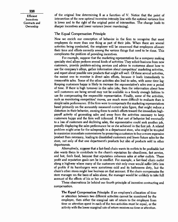
228



of the original line determining B as a function of V. Notice that the point of intersection of the new optimal incentive-intensity line with the optimal variance line is lower and to the right of the original point of intersection. The change leads to sharper incentives and lower variance (more monitoring).

The Equal Compensation Principle

Now we enrich our conception of behavior in the firm to recognize that most employees do more than one thing as part of their jobs. When there are several activities being conducted, the employer will be concerned that employees allocate their time and efforts correctly among the various things that need to be done. This complicates the problem of providing incentives.

For example, suppose that the marketing representatives for a company making specialty steel alloys perform several kinds of activities: They solicit business from new customers, provide problem-solving services and advice to customers about how to use the company's alloys, gather information about competitors' marketing activities, and report about possible new products that might sell well. Of these several activities, the easiest one to monitor is direct sales efforts, because it leads immediately to measurable sales. Some of the other activities also lead to sales, with some time lag: Keeping customers happy is likely to increase the representative's sales over a period of time. If there is high turnover in the sales jobs, then the information about how well customers are being served may not be available in a timely enough fashion to use for compensating the responsible representative. Finally, some of the activities, such as monitoring competitors' moves, are much more difficult to evaluate than is simple sales performance. If the firm were to compensate the marketing representatives based primarily on the accurately measured current sales figure, that might induce a distortion in their behavior, causing them to switch efforts toward the immediate high-payoff activity of generating sales and away from the activities necessary to keep customers happy and the firm well informed. If that sort of behavior led eventually to a loss of customers and declining sales, the representative could seek another job, proudly displaying the sales performance he or she achieved in the first job. A related problem might arise for the salespeople in a department store, who might be tempted to maximize immediate commissions by pressuring a customer to buy a more expensive product than necessary, leading to dissatisfied customers and lower future sales for the store, not only of that one department's products but also of products sold in other departments.

Alternatively, suppose that a fast-food chain wants its outlets to be profitable but also wants them to contribute to the chain's reputation for cleanliness, fast service, and hot, fresh food, because that reputation enhances sales at other outlets. These profit and reputation goals can be in conflict. For example, a fast-food chain outlet along a highway where many of the customers visit only once would suffer little loss of profits if its hamburgers were sometimes cold and its bathrooms dirty, but the chain's other stores might lose business on that account. If the chain compensates the store manager on the basis of sales alone, the manager would be unlikely to take full account of the effects of his or her actions.

These observations lie behind our fourth principle of incentive contracting and compensation.

The Equal Compensation Principle: If an employee's allocation of time or attention between two different activities cannot be monitored by the employer, then either the marginal rate of return to the employee from time or attention spent in each of the two activities must be equal, or the activity with the lower marginal rate of return receives no time or attention,

229

The equal compensation principle imposes a serious constraint on the incentive-compensation formulas that can be effective in practice. In particular, if an employee is expected to devote time and effort to some activity for which performance cannot be measured at all (V = co), then incentive pay cannot be effectively used for any other activities that the individual controls. The use of straight salary compensation for managers can often be justified on these grounds.

MATHEMATICS OF THE EQUAL COMPENSATION PRINCIPLE Suppose the employee does two different things, signified by levels of effort e l and e2 . We will think of these levels of effort as time devoted to two activities, and we assume that the cost incurred by the employee is an opportunity cost: It is time that becomes unavailable for other, more pleasant or rewarding activities. It then makes sense to write the cost as depending only on the total effort, not on its division between the two tasks: C(e l + e2). The employer measures performance by observing the indicators e i + xi and e2 + x2 , where x t and x2 have expected values of 1 1 and Iv

Suppose that the employer pays the employee according to a linear compensation formula based on the two indicators: The wage paid is then w = a + 13 1 (e1 + xi ) + B2(e2 +x2). How should a, B 1 , Bb e l , and e 2 be chosen?

To take incentives into account in the problem, we first examine the employee's objective given this compensation rule. A self-interested employee will choose e l and e2 to maximize his or her certain equivalent income:

Employee's Certain Equivalent = a + 81 (e 1 + + B 2(e2 + F2) — C(e i + ez ) rVar(B ix i + 132x2) (7.10)

For this problem, we suppose that the effort is restricted to a nonnegative number: e l , e2 0. If e l is strictly positive, then at the maximizing choice for the employee, the derivative of Equation 7.10 with respect to e l must be zero, so 13 1 = C'(e l + e2 ). Similarly, if e 2 is strictly positive, then B 2 = Ci(e i + e2). The analysis of the employee's incentives alone thus establishes that 13 1 must equal B2 if each tasks is to receive some attention.

APPLICATION: COST CENTERS AND PROFIT CENTERS As the models make clear, an important part of the problem of designing incentives is to determine what the employee will be responsible for, that is, what measures will be used to evaluate performance as a basis for compensation. As an example, consider the problem of providing incentives to the manager of a manufacturing facility. One approach might declare that the manager is responsible only for the costs incurred in the factory, on the theory that the manager has little control over revenues. In that case, we say that the factory is a cost center, and the accounting systems should be set up to assess accurately the costs attributable to the factory. Another approach declares that product quality and speed of delivery are important to sales, so that it is a mistake to encourage the manager to focus on cost control at the expense of these factors. Thus, sales performance might be given some weight in determining the manager's compensation.

To represent these issues in terms of our theory, suppose that the two activities to which the manager might contribute are cost reduction and revenue generation. If sales revenues are subject to random variations that are outside the manager's control and statistically independent of the randomness that affects costs, then the cost of providing incentives of strength 13 to the manager for revenue generation is the risk premium: 4 r13 2Var(Revenues). The equal compensation principle implies that if the factory manager is to be provided with sales-generation incentives at all, then it is futile to do that in a half-hearted way: The incentives need to be of the same strength as those for manufacturing cost control. If the B associated with cost control is to be large, then the 13 associated with revenue generation must be large as well, and


230

fficient therefore quite costly (in the sense of its leading to a large risk premium). Then, the E

Incentivm factory is a profit center, to which revenues and costs are both attributed in determining Contracts and performance.

Ownership Cost centers and profit centers are not the only alternatives, however, nor is either likely to be the best alternative in the situation we have described. The firm should actively seek ways to make production managers responsible for what they each control without making them responsible for the performance of the sales force, which they do not control. For example, if quality control and delays in the factory are the chief concerns, then the firm could devise new measures of manufacturing perfor-mance, such as the average time from order to delivery and the number of products returned as unsatisfactory. According to the informativeness principle, these measures are superior to measures based on dollar sales because they provide a more informative assessment of the manufacturing manager's actual contribution to the sales effort. As we observed earlier, the firm gains most by improving the measurement of variables that figure most heavily as a basis for compensation.

The equal compensation principle suggests another possibility as well: The manager could be paid a salary with no explicit incentive component. This would be a plausible course of action when manufacturing quality control is important but hard to assess accurately. Of course, the manager will still understand that promotions and pay increases will depend on how superiors assess his or her performance, but at least this solution avoids the distortions in allocation of time and effort and the randomness in compensation brought about by an incentive compensation plan based on arbitrary measures of performance.

This analysis of cost and profit centers focuses only on the issue of compensation. Before leaving this example, however, it is helpful to recall that the actual organization design problem is more involved than that. Managers who are given responsibility for profits, for example, are commonly given broader decision authority than those responsible just for costs or sales. Determining a manager's compensation amounts to deciding what he or she is responsible for, and that decision should be made together with decisions about the scope of the manager's authority.

APPLICATION: INCENTIVES FOR TEACI IERS The equal compensation principle can be applied to the recent public policy debate about whether it would be helpful to provide cash incentives for teachers to improve elementary and secondary education. Proponents of cash incentives argue that they would be helpful in focusing teachers on their tasks and motivating them to be innovative in the search for effective ways to train their students.

Opponents of the incentives for teachers, however, have a cogent response. The measures that have been used in the past to evaluate teaching performance for elementary school age children are tests of basic skills, and teaching these is just one part of a teacher's job. Children are also expected to learn social skills, oral expression, and creative thinking, and to build confidence that prepares them for the harder challenges to be faced in later years. Teachers who are compensated based on tests of basic skills alone would be tempted to neglect these other aspects of the job. They might also be led to teaching the most docile students, whose performance scores are easiest to improve, while neglecting students who have more trouble learning. In one instance in South Carolina in 1989, a teacher was caught teaching the answers to the actual test, a copy of which had been illicitly obtained. Compensating teachers based on test scores motivates teachers to help students test well, rather than to help students learn.

According to the equal compensation principle, if it is desirable to have teachers devote some efforts to each of several activities and if it is impossible to distinguish

efforts on the various different activities, then all these kinds of efforts must be compensated equally. If social development, oral expression, or creative thinking cannot be accurately measured, then the only realistic options are to remove the responsibility for teaching them from the teacher or to pay the teacher a fixed wage, with no element of incentives pay.

It is a good idea to remember that responsibilities and compensation should really be determined together. In the case of teachers, for example, one proposal is to install a system of specialist teachers who are compensated based on student test scores but who are not responsible for other aspects of student performance. 7 This would not, by itself, solve all the potential problems we have described, but it would allow performance incentives and still ensure that attention is paid to developing the very important "higher thinking skills" in young students. The general point to remember is that by determining the job design and the compensation together, one can sometimes solve problems that cannot be solved by compensation policy alone.

APPLICATION: ASSET OWNERSHIP The equal compensation principle also makes it possible to give a careful treatment of some important issues in the theory of employment and asset ownership. We represent ownership by supposing that at the end of a period of production, the owner of the asset may take it and employ it in other uses. For example, if the employer is the owner of a machine (the asset), he or she can assign the job of production and the use of the asset to another worker, whereas if the worker owns the asset then he or she can employ it on his or her own behalf or on behalf of another employer. What kind of incentives are optimal and who should own the asset?

Assets are notoriously hard to evaluate accurately and objectively. That is why accountants generally report adjusted historical cost figures for asset valuations rather than attempting to account for asset values on the basis of the asset's physical condition (unless deterioration is obvious), its fair market value, or its productivity. The value of a business automobile, for example, is accounted for by its purchase price less an allowance for depreciation, even though its actual value depends on its mileage, physical condition, and so on. Production machines are accounted for in a similar way, even if hard use or changes in production methods has made their actual value lower.

We represent the idea that assets are hard to value accurately in our model by the following assumption: Although the actual value of the asset, A(e l ) + xi , is an increasing function of the effort e l that the worker devotes to maintaining and improving the asset (and of random factors x i ), accounting measures of asset values do not reflect those efforts and so cannot be used to provide incentives. Only the direct output of the production process, which is e 2 + x2, is observed by the parties and can serve as a basis for compensation. Therefore, we may write the compensation paid to the worker in the form a + B(e 2 + x2).

Suppose that there is some level of total effort F that the employee is willing to provide even in the absence of any cash incentives, although this level might be lower than the employer would like to see provided. The efforts e, and e2 devoted to each of the two activities cannot be observed, however. Should the firm induce greater effort by setting B positive and thereby inducing more production effort e 2?

If the firm owns the asset, then the worker's certain equivalent compensation is + Be 2 — 4nVar(x 2) — C(e i + e2). If B is positive, the worker's optimal choice of

el is always zero. This is just an application of the equal compensation principle:

7 Jane Hannaway, "Higher Order Skills, Job Design, and Incentives: An Analysis and Proposal,' working paper, Stanford University, 1991.

231


232

Efficient Because the marginal return to the agent from efforts devoted to maintaining or

Incentives: increasing the asset's value is always zero, the worker will devote no efforts to that Contracts and act;vity (e l = 0) unless the returns to other activities are also zero. When the worker

Ownership is an employee and maintenance of the asset is important, we find (in this model) that it is optimal to pay a fixed wage with no incentives for output performance (13 = 0). Then the worker will set e l + e2 = I and presumably will be willing to allocate this total amount of effort as the firm directs.

The other possibility is that the worker may own the asset. In that case, the worker's certain equivalent compensation is the sum of the asset's expected value (which depends on e l ) and his or her expected compensation, less a risk premium that reflects both the uncertainty in the asset's value and that in the worker's pay, as well as the cost of effort: A(e l ) + a + Be2 — irVar(x 1 + Bx 2 ) — C(ei + ez ). As the owner, the worker has a built-in incentive to care for the asset; he or she keeps any value that is created when the asset is well cared for. In order to motivate the worker also to pay some attention to production, it is necessary to set 3 > 0. Then, with positive returns to both types of effort, the worker will choose to provide more total effort than I—the amount he or she would provide as an employee with no pay incentives for working harder.

■ To summarize, if it is important that time and effort be devoted to both /producing and maintaining the asset, then incentive pay should always be used for

workers who bring their own tools ("independent contractors"), but it should never be used for those who use the firm's tools ("employees"). In practice, incentives are used more extensively for independent contractors than for individual employees, as our analysis suggests they should be. The analysis also suggests that independent contractors will work harder than employees, devoting more effort both to caring for the asset and to being directly productive. They will also earn a higher average income to compensate for the extra work they do and the greater risk they bear.

Finally, we come to the question: Who should own the asset? A detailed study of asset ownership is contained in Chapter 9, so we are brief here. In the model just described, if the worker owns the asset, then the worker bears risk both from the randomness of asset returns and from the errors in performance measurement, which add 4r(132Var(x2) + Var(x 1 )) to the total risk premium. Against this must be weighed the fact that the ownership of the asset and increased incentives for the production activity will elicit a higher level of effort. A cost-benefit calculation that balances these considerations must be done to determine which arrangement is likely to be more successful. Certain genera] principles are evident, however. Increases in the worker's risk aversion or in the variance of asset returns or in the variance of performance estimates in the production task all add to the risk premium that is incurred when the employee owns the asset, making the ownership solution less valuable. If there are many ways to improve performance, then the employee's efforts are especially likely to be responsive to incentives (represented in our model by the assumption that C" is small). Increases in the worker's scope for action tend to favor having the worker own the asset. As we see later, there are a number of other considerations involved in assigning asset ownership efficiently that are not represented in this simple conceptual model.

milgrom and roberts, “risk sharing and incentive contracts,”

Documents