millennials: the housing edition

August 4, 2014

Thematic Research

Millennials: The Housing Edition

Equity Research

Out of basements and into homes

A Millennial refresh

Millennials are one of the biggest generations in US

history and are comprised of individuals born

between 1980 and 2000. Millennials are more

diverse, more educated, more in debt and more

likely to be in the South and West. The peak

millennial cohort is now only 23 years old. Because

housing consumption increases sharply from age 25

to 45, millennials will be an important factor for the

broader housing market going forward.

Large numbers will overpower restraints

While there are several impediments to

homeownership (tight credit, lack of affordable

inventory, elevated debt levels) we believe the

sheer size of the millennial cohort can drive

increased demand for housing.

Plans to marry, own and have kids

Generally, millennials want many of the same

things as previous generations. However, life

events such as marriage and having children are

being pushed back for this group.

Divergence of fortunes raises concerns

The biggest challenge faced by millennials is weak

income growth among those without college

degrees – a structural risk if not addressed. The

decline in interest rates over the past 30 years has

compensated for the decline in real income for

those without college degrees. However, if their

real income declines further or interest rates

increase, homeownership could become

increasingly unaffordable.

Prefer college even with some debt

We find it takes at least $50,000 in student debt or

student debt payments of at least 5% of income to

have a significant impact on homeownership.

While these buckets have been growing they still

represent a small share of the population.

Improvement in credit is key

There has been limited easing of credit standards.

Given that young adults tend to have the weakest

credit, opening of the credit box should have the

most positive impact on this group.

Eli Hackel, CFA

(212) 902-9672 [email protected] Goldman, Sachs & Co.

Hui Shan

(212) 902-4447 [email protected] Goldman, Sachs & Co.

Goldman Sachs does and seeks to do business with companies covered in its research reports. As a result, investors should be aware that the firm may have a conflict of interest that could affect the objectivity of this report. Investors should consider this report as only a single factor in making their investment decision.For Reg AC certification and other important disclosures, see the Disclosure Appendix, or go to www.gs.com/research/hedge.html. Analysts employed by non-US affiliates are not registered/qualified as research analysts with FINRA in the U.S.

The Goldman Sachs Group, Inc. Global Investment Research

August 4, 2014 Americas

Goldman Sachs Global Investment Research 2

Millennial’s housing demand on the rise, lack of income growth is our biggest concern

Millennials (born 1980-2000) are one of the biggest generations in U.S. history with 82 million born in the US during these years. As they move into a life cycle

stage when housing consumption increases sharply, their housing demand could be influential to the US housing outlook.

While the media inundates us with stories about ballooning student loans, recent college graduates having difficulties finding decent jobs, and young adults

living with their parents, we believe there should be increasing demand for housing from millennials. We show, even in a pessimistic scenario analysis, to

expect household formation of a minimum of 1mn, starts of at least 1.2mn/1.3mn, and new home sales climbing to 650K in the coming years. As a comparison,

GS baseline forecasts point to 1.5mn housing starts and 740K new home sales in 2017.

We use a framework where all relevant drivers are divided into internal factors—life cycle, income, personal finance, attitude and preferences—and external

factors—the availability of jobs, mortgages and affordable homes. We bring evidence from micro data and examine these drivers in turn.

Millennials demand for housing will increase even with constraints:

The biggest challenge faced by millennials, in our view, is weak income growth among those lacking college degrees. Declining mortgage interest rates

over the past three decades have offset the negative impact from falling income and rising house prices. But interest rates are more likely to rise than to

fall going forward (GS economics forecasts 10-year Treasury yields increase from 2.5% currently to 4.0% by the end of 2017), raising the question

whether this group will be able to afford buying homes if their income keeps declining and house prices continue to increase.

However, the sheer size of the millennial cohort compensates for the challenges faced by young adults. Even assuming no improvement in the headship

rate and homeownership rate among young adults, we still expect recovery, albeit a slower one, in the housing market. In addition, we expect continued

job growth and gradual easing of mortgage standards (GS economics projects the unemployment rate falls to 4.8% in 2017 from 6.2% currently), both of

which are positive forces for the housing market.

Key findings of our analysis:

Millennials marry and have children later in life than earlier generations, but they expect to eventually marry and have children (see pages 6-7 for more

detail).

We find little evidence that young renters do not want to be homeowners anymore post crisis. However, there is some evidence that young homeowners

increasingly prefer multi-family housing and living closer to work (see page 8 for more detail).

Median income hides the diverging fortunes of college graduates and the less well educated. Young individuals with high school degrees or less face

falling income and declining homeownership rate (see page 9 for more detail).

Borrowing money for college has costs and benefits when it comes to housing consumption. The benefits outweigh the costs as long as the debt burden

is not too large, the borrower finishes college, and the college degree offers better income prospects (see pages 12-13 for more detail).

Tight mortgage credit hurts young individuals the most as they are likely to have low credit scores. Fear of being turned down, many individuals with low

credit scores no longer apply for mortgages, which depresses housing demand (see page 14 for more detail).

House price appreciation has outpaced income growth over the past 15 years. The lack of affordable entry-level homes on the market is a headwind to

the millennials’ homeownership rate (see page 16 for more detail).

Labor market conditions continue to improve and wage inflation should slowly pick up. Young individuals are also more optimistic about future income

growth. These are positive signs for housing demand (see page 17 for more detail).



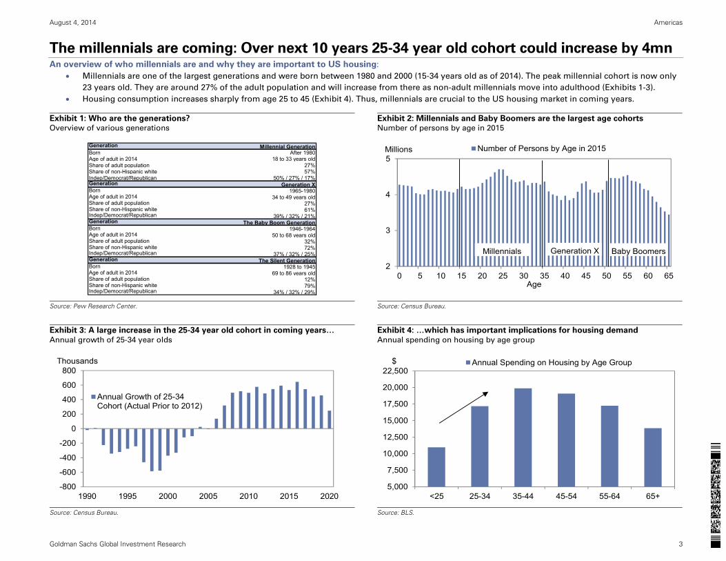
The millennials are coming: Over next 10 years 25-34 year old cohort could increase by 4mn An overview of who millennials are and why they are important to US housing:

Millennials are one of the largest generations and were born between 1980 and 2000 (15-34 years old as of 2014). The peak millennial cohort is now only

23 years old. They are around 27% of the adult population and will increase from there as non-adult millennials move into adulthood (Exhibits 1-3).

Housing consumption increases sharply from age 25 to 45 (Exhibit 4). Thus, millennials are crucial to the US housing market in coming years.

Exhibit 1: Who are the generations? Overview of various generations

Exhibit 2: Millennials and Baby Boomers are the largest age cohorts Number of persons by age in 2015

Source: Pew Research Center.

Source: Census Bureau.

Exhibit 3: A large increase in the 25-34 year old cohort in coming years…

Annual growth of 25-34 year olds

Exhibit 4: …which has important implications for housing demand

Annual spending on housing by age group

Source: Census Bureau.

Source: BLS.

Generation Millennial GenerationBorn After 1980Age of adult in 2014 18 to 33 years oldShare of adult population 27%Share of non-Hispanic white 57%Indep/Democrat/Republican 50% / 27% / 17%Generation Generation XBorn 1965-1980Age of adult in 2014 34 to 49 years oldShare of adult population 27%Share of non-Hispanic white 61%Indep/Democrat/Republican 39% / 32% / 21%Generation The Baby Boom GenerationBorn 1946-1964Age of adult in 2014 50 to 68 years oldShare of adult population 32%Share of non-Hispanic white 72%Indep/Democrat/Republican 37% / 32% / 25%Generation The Silent GenerationBorn 1928 to 1945Age of adult in 2014 69 to 86 years oldShare of adult population 12%Share of non-Hispanic white 79%Indep/Democrat/Republican 34% / 32% / 29%

2

3

4

5

0 5 10 15 20 25 30 35 40 45 50 55 60 65

Millions

Age

Number of Persons by Age in 2015

Millennials Baby BoomersGeneration X

-800

-600

-400

-200

0

200

400

600

800

1990 1995 2000 2005 2010 2015 2020

Thousands

Annual Growth of 25-34Cohort (Actual Prior to 2012)

5,000

7,500

10,000

12,500

15,000

17,500

20,000

22,500

<25 25-34 35-44 45-54 55-64 65+

$ Annual Spending on Housing by Age Group



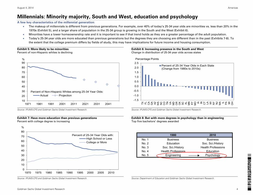
Millennials: Minority majority, South and West, education and psychology A few key characteristics of the millennial generation:

The makeup of millennials is different from previous generations. For example, over 40% of today’s 25-34 year olds are minorities vs. less than 20% in the

1970s (Exhibit 5), and a larger share of population in the 25-34 group is growing in the South and the West (Exhibit 6).

Minorities have a lower homeownership rate and it is important to see if that trend holds as they are a greater percentage of the adult population.

Today’s 25-34 year olds are more educated than previous generations but the degrees they are choosing are different than in the past (Exhibits 7-8). To

the extent that the college premium differs by fields of study, this may have implications for future income and housing consumption.

Exhibit 5: More likely to be minorities Percent of non-Hispanic whites is declining

Exhibit 6: Increasing presence in the South and West Change in distribution of 25-34 year olds across states

Source: IPUMS-CPS and Goldman Sachs Global Investment Research.


Exhibit 7: Have more education than previous generations Percent with college degree is increasing

Exhibit 8: But with more degrees in psychology than in engineering Top five bachelors’ degrees awarded


Source: Department of Education and Goldman Sachs Global Investment Research.

10

20

30

40

50

60

70

80

90

1971 1981 1991 2001 2011 2021 2031 2041

%

Actual ProjectionPercent of Non-Hispanic Whites among 25-34 Year Olds:

-1.5

-1.0

-0.5

0.0

0.5

1.0

1.5

2.0

2.5

TX FL CA

GA AZ WA

NC

CO TN VA MD

OR

OK

SC AL MN KY MO IA IN CT LA WI

NY NJ

MA IL PA MI

OH

Percent of 25-34 Year Olds in Each State(Change from 1980s to 2010s)

Percentage Points

0

10

20

30

40

50

60

70

80

1970 1975 1980 1985 1990 1995 2000 2005 2010

%

High School or LessCollege or More

Percent of 25-34 Year Olds with: 1980 2010No. 1 Business BusinessNo. 2 Education Soc. Sci./HistoryNo. 3 Soc. Sci./History Health ProfessionsNo. 4 Health Professions EducationNo. 5 Engineering Psychology



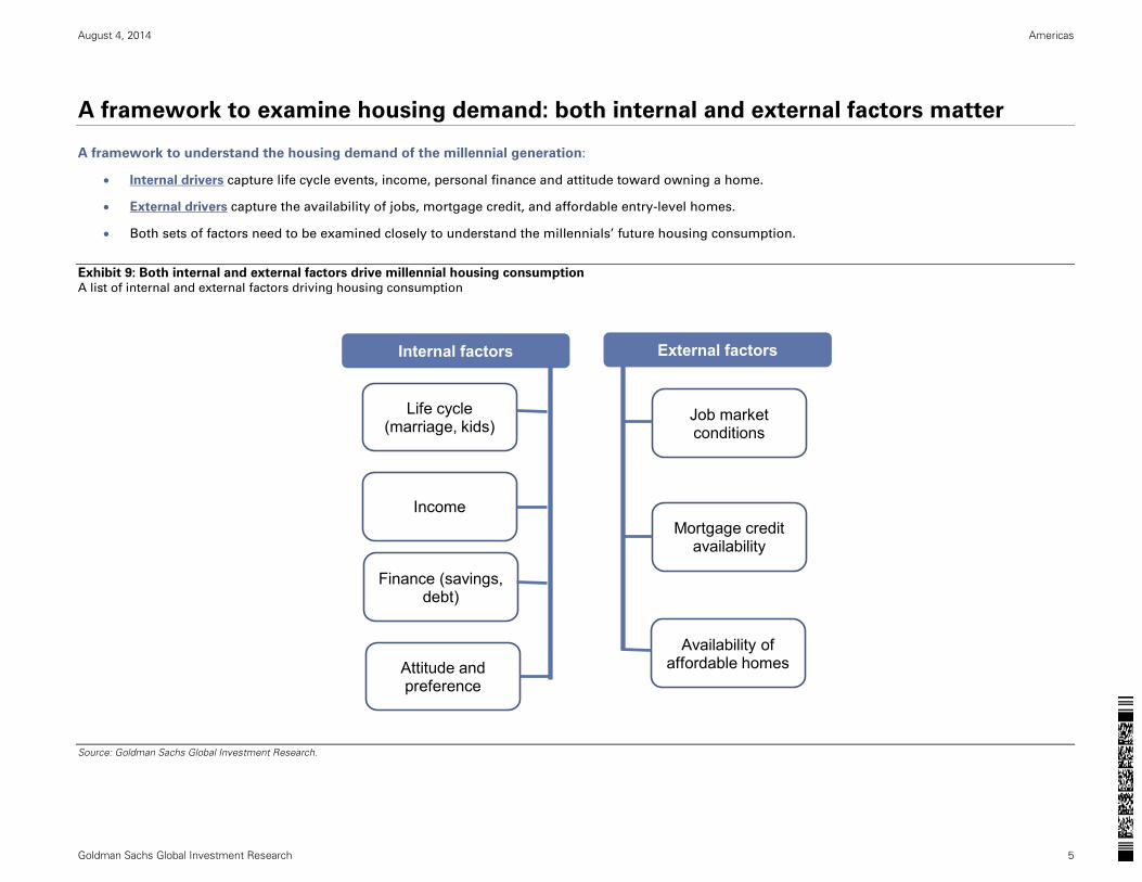
A framework to examine housing demand: both internal and external factors matter

A framework to understand the housing demand of the millennial generation:

Internal drivers capture life cycle events, income, personal finance and attitude toward owning a home.

External drivers capture the availability of jobs, mortgage credit, and affordable entry-level homes.

Both sets of factors need to be examined closely to understand the millennials’ future housing consumption.

Exhibit 9: Both internal and external factors drive millennial housing consumption A list of internal and external factors driving housing consumption

Source: Goldman Sachs Global Investment Research.

Internal factors

Life cycle (marriage, kids)

Income

Finance (savings, debt)

Attitude and preference

External factors

Job market conditions

Mortgage credit availability

Availability of affordable homes



A delayed life cycle is pushing back household formation and homeownership… Americans’ life cycle has been changing:

Individuals are getting married later, having children later, living with their parents for longer, and buying homes at an older age. For example, the

median marriage age has increased from 23 in the 1970s to 30 in the 2010s (Exhibits 10-13).

The recent weakness in household formation results from both secular trends and the lingering effect of the recession. We believe the latter should fade

over time. However, there could be changing preferences and increasing acceptance of living at home for longer.

Exhibit 10: Marriage age has been pushed back in the last few decades… Median marriage age increased from 23 in 1970s to 30 in 2010s

Exhibit 11: …and also child-bearing age Peak child-bearing age increased from 24 in 1970s to 28 in 2010s



Exhibit 12: Long trend of delaying independent living Fewer 25-34 year olds live independently over time

Exhibit 13: Homeownership is also delayed Median age when buying first home increased from 29 in 1970s to 33 in 2010s



0102030405060708090

15 25 35 45 55 65

%

1970s 1980s 1990s2000s 2010s

Age

Percent of Married Individuals by Age:

0

2

4

68

10

12

1416

15 20 25 30 35 40 45

%

1970s 1980s1990s 2000s2010s

Age

Percent of Women Having Children by Age:

0%10%20%30%40%50%60%70%80%90%

100%

1970s 1980s 1990s 2000s 2010s

Non-Relatives

Relatives

Parents

Self/Spouse

Fraction of 25-34 Year Olds

Living with:

102030405060708090

20 25 30 35 40 45 50 55 60

%

1970s 1980s 1990s2000s 2010s

Homeownership Rate by Age:

Age



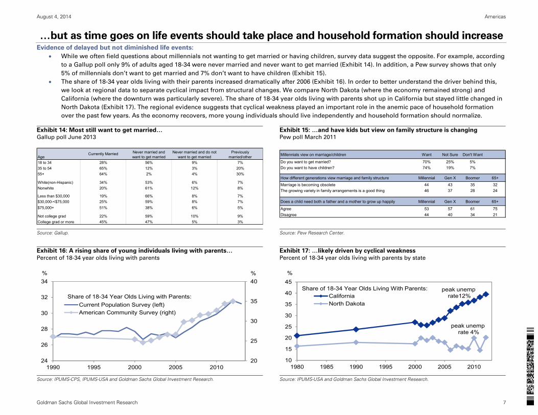
…but as time goes on life events should take place and household formation should increase Evidence of delayed but not diminished life events:

While we often field questions about millennials not wanting to get married or having children, survey data suggest the opposite. For example, according

to a Gallup poll only 9% of adults aged 18-34 were never married and never want to get married (Exhibit 14). In addition, a Pew survey shows that only

5% of millennials don’t want to get married and 7% don’t want to have children (Exhibit 15).

The share of 18-34 year olds living with their parents increased dramatically after 2006 (Exhibit 16). In order to better understand the driver behind this,

we look at regional data to separate cyclical impact from structural changes. We compare North Dakota (where the economy remained strong) and

California (where the downturn was particularly severe). The share of 18-34 year olds living with parents shot up in California but stayed little changed in

North Dakota (Exhibit 17). The regional evidence suggests that cyclical weakness played an important role in the anemic pace of household formation

over the past few years. As the economy recovers, more young individuals should live independently and household formation should normalize.

Exhibit 14: Most still want to get married… Gallup poll June 2013

Exhibit 15: …and have kids but view on family structure is changing Pew poll March 2011

Source: Gallup.

Source: Pew Research Center.

Exhibit 16: A rising share of young individuals living with parents…

Percent of 18-34 year olds living with parents

Exhibit 17: …likely driven by cyclical weakness

Percent of 18-34 year olds living with parents by state

Source: IPUMS-CPS, IPUMS-USA and Goldman Sachs Global Investment Research.

Source: IPUMS-USA and Goldman Sachs Global Investment Research.

Age18 to 34 28% 56% 9% 7%35 to 54 65% 12% 3% 20%55+ 64% 2% 4% 30%

White(non-Hispanic) 34% 53% 6% 7%Nonwhite 20% 61% 12% 8%

Less than $30,000 19% 66% 8% 7%$30,000-<$75,000 25% 59% 8% 7%$75,000+ 51% 38% 6% 5%

Not college grad 22% 59% 10% 9%College grad or more 45% 47% 5% 3%

Previously married/other

Currently Married Never married and want to get married

Never married and do not want to get married Millennials view on marriage/children Want Not Sure Don't Want

Do you want to get married? 70% 25% 5%Do you want to have children? 74% 19% 7%

How different generations view marriage and family structure Millennial Gen X Boomer 65+

Marriage is becoming obsolete 44 43 35 32The growing variety in family arrangements is a good thing 46 37 28 24

Does a child need both a father and a mother to grow up happily Millennial Gen X Boomer 65+

Agree 53 57 61 75Disagree 44 40 34 21

20

25

30

35

40

24

26

28

30

32

34

1990 1995 2000 2005 2010

%%

Current Population Survey (left)American Community Survey (right)

Share of 18-34 Year Olds Living with Parents:

10

15

20

25

30

35

40

45

1980 1985 1990 1995 2000 2005 2010

%

CaliforniaNorth Dakota

Share of 18-34 Year Olds Living With Parents: peak unemp rate12%

peak unemp rate 4%



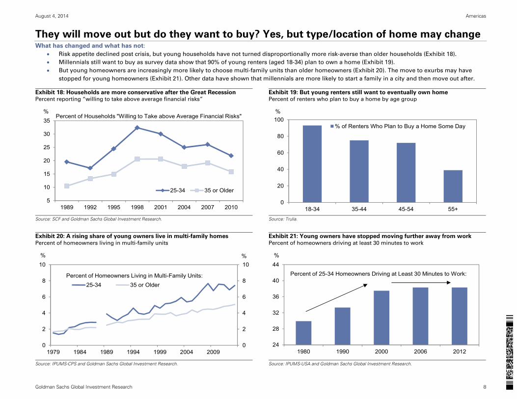
They will move out but do they want to buy? Yes, but type/location of home may change What has changed and what has not:

Risk appetite declined post crisis, but young households have not turned disproportionally more risk-averse than older households (Exhibit 18).

Millennials still want to buy as survey data show that 90% of young renters (aged 18-34) plan to own a home (Exhibit 19).

But young homeowners are increasingly more likely to choose multi-family units than older homeowners (Exhibit 20). The move to exurbs may have

stopped for young homeowners (Exhibit 21). Other data have shown that millennials are more likely to start a family in a city and then move out after.

Exhibit 18: Households are more conservative after the Great Recession Percent reporting “willing to take above average financial risks”

Exhibit 19: But young renters still want to eventually own home Percent of renters who plan to buy a home by age group

Source: SCF and Goldman Sachs Global Investment Research.

Source: Trulia.

Exhibit 20: A rising share of young owners live in multi-family homes Percent of homeowners living in multi-family units

Exhibit 21: Young owners have stopped moving further away from work Percent of homeowners driving at least 30 minutes to work



5

10

15

20

25

30

35

1989 1992 1995 1998 2001 2004 2007 2010

%

25-34 35 or Older

Percent of Households "Willing to Take above Average Financial Risks"

0

20

40

60

80

100

18-34 35-44 45-54 55+

%

% of Renters Who Plan to Buy a Home Some Day

0

2

4

6

8

10

0

2

4

6

8

10

1979 1984 1989 1994 1999 2004 2009

%%

25-34 35 or OlderPercent of Homeowners Living in Multi-Family Units:

24

28

32

36

40

44

1980 1990 2000 2006 2012

%

Percent of 25-34 Homeowners Driving at Least 30 Minutes to Work:



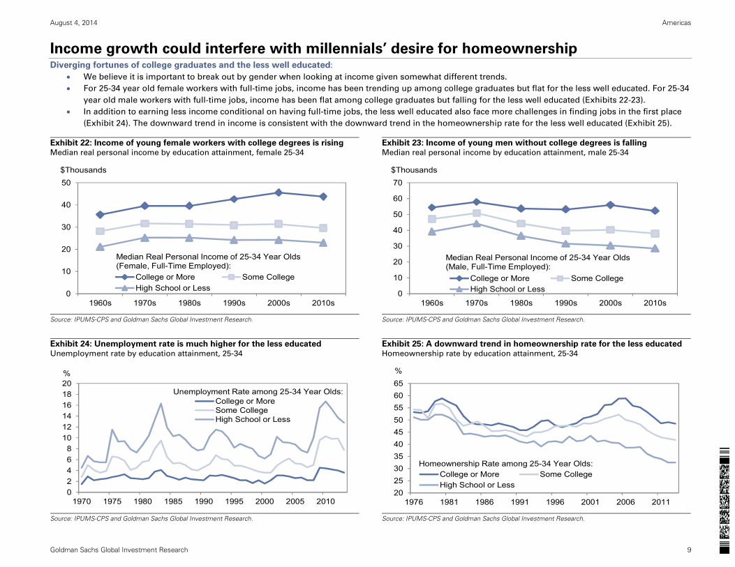
Income growth could interfere with millennials’ desire for homeownership Diverging fortunes of college graduates and the less well educated:

We believe it is important to break out by gender when looking at income given somewhat different trends.

For 25-34 year old female workers with full-time jobs, income has been trending up among college graduates but flat for the less well educated. For 25-34

year old male workers with full-time jobs, income has been flat among college graduates but falling for the less well educated (Exhibits 22-23).

In addition to earning less income conditional on having full-time jobs, the less well educated also face more challenges in finding jobs in the first place

(Exhibit 24). The downward trend in income is consistent with the downward trend in the homeownership rate for the less well educated (Exhibit 25).

Exhibit 22: Income of young female workers with college degrees is rising Median real personal income by education attainment, female 25-34

Exhibit 23: Income of young men without college degrees is falling Median real personal income by education attainment, male 25-34



Exhibit 24: Unemployment rate is much higher for the less educated Unemployment rate by education attainment, 25-34

Exhibit 25: A downward trend in homeownership rate for the less educated Homeownership rate by education attainment, 25-34



0

10

20

30

40

50

1960s 1970s 1980s 1990s 2000s 2010s

$Thousands

College or More Some CollegeHigh School or Less

Median Real Personal Income of 25-34 Year Olds(Female, Full-Time Employed):

0

10

20

30

40

50

60

70

1960s 1970s 1980s 1990s 2000s 2010s

$Thousands


Median Real Personal Income of 25-34 Year Olds(Male, Full-Time Employed):

02468

101214161820

1970 1975 1980 1985 1990 1995 2000 2005 2010

%

College or MoreSome CollegeHigh School or Less

Unemployment Rate among 25-34 Year Olds:

20253035404550556065

1976 1981 1986 1991 1996 2001 2006 2011

%


Homeownership Rate among 25-34 Year Olds:



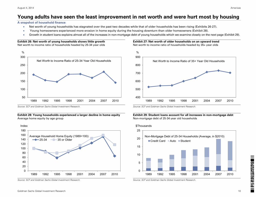
Young adults have seen the least improvement in net worth and were hurt most by housing A snapshot of household finance:

Net worth of young households has stagnated over the past two decades while that of older households has been rising (Exhibits 26-27).

Young homeowners experienced more erosion in home equity during the housing downturn than older homeowners (Exhibit 28).

Growth in student loans explains almost all of the increases in non-mortgage debt of young households which we examine closely on the next page (Exhibit 29).

Exhibit 26: Net worth of young households shows little growth Net worth to income ratio of households headed by 25-34 year olds

Exhibit 27: Net worth of older households on an upward trend Net worth to income ratio of households headed by 35+ year olds



Exhibit 28: Young households experienced a larger decline in home equity

Average home equity by age group

Exhibit 29: Student loans account for all increases in non-mortgage debt

Non-mortgage debt of 25-34 year old households



50

100

150

200

250

300

1989 1992 1995 1998 2001 2004 2007 2010

%

Net Worth to Income Ratio of 25-34 Year Old Households

400

500

600

700

800

900

1989 1992 1995 1998 2001 2004 2007 2010

%

Net Worth to Income Ratio of 35+ Year Old Households

020406080

100120140160180

1989 1992 1995 1998 2001 2004 2007 2010

Index

25-34 35 or OlderAverage Household Home Equity (1989=100):

0

5

10

15

20

25

1989 1992 1995 1998 2001 2004 2007 2010

$Thousands

Credit Card Auto StudentNon-Mortgage Debt of 25-34 Households (Average, in $2010)



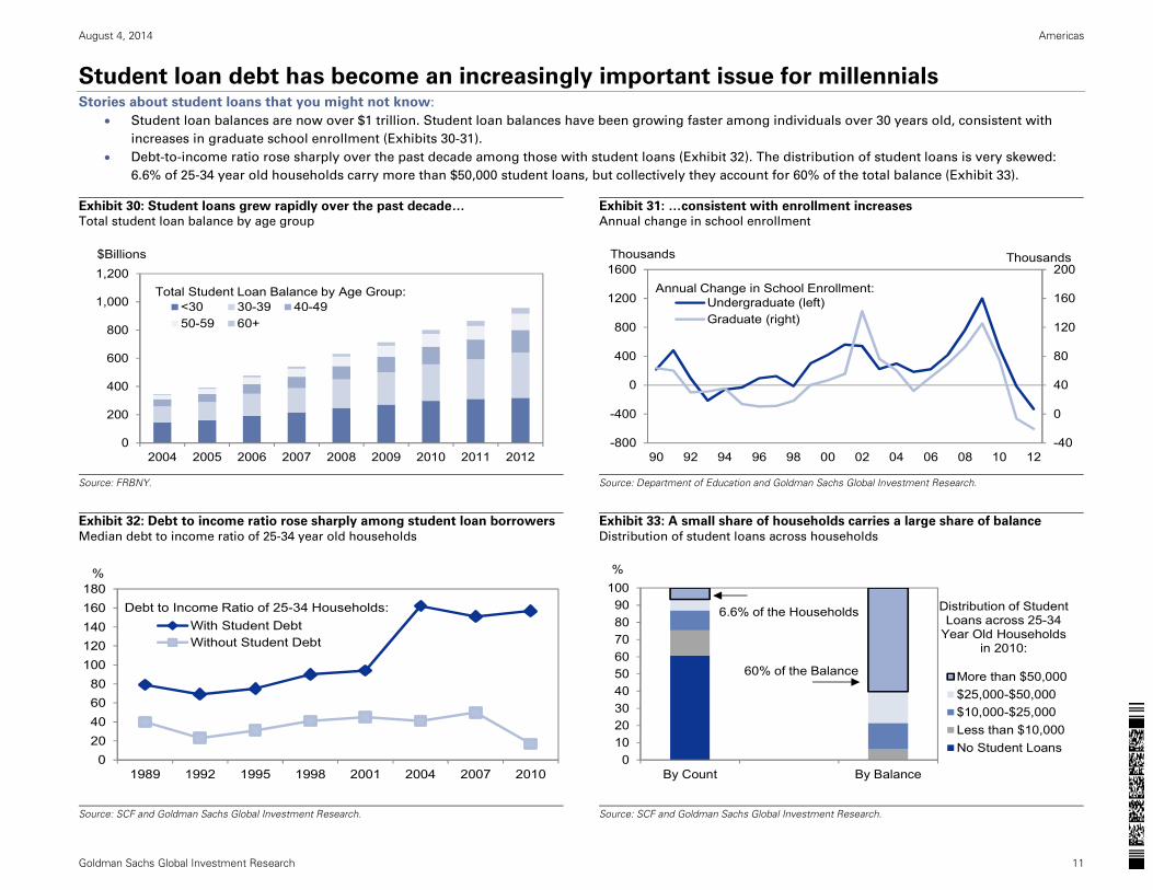
Student loan debt has become an increasingly important issue for millennials Stories about student loans that you might not know:

Student loan balances are now over $1 trillion. Student loan balances have been growing faster among individuals over 30 years old, consistent with

increases in graduate school enrollment (Exhibits 30-31).

Debt-to-income ratio rose sharply over the past decade among those with student loans (Exhibit 32). The distribution of student loans is very skewed:

6.6% of 25-34 year old households carry more than $50,000 student loans, but collectively they account for 60% of the total balance (Exhibit 33).

Exhibit 30: Student loans grew rapidly over the past decade… Total student loan balance by age group

Exhibit 31: …consistent with enrollment increases Annual change in school enrollment

Source: FRBNY.

Source: Department of Education and Goldman Sachs Global Investment Research.

Exhibit 32: Debt to income ratio rose sharply among student loan borrowers

Median debt to income ratio of 25-34 year old households

Exhibit 33: A small share of households carries a large share of balance

Distribution of student loans across households



0

200

400

600

800

1,000

1,200

2004 2005 2006 2007 2008 2009 2010 2011 2012

$Billions

<30 30-39 40-4950-59 60+

Total Student Loan Balance by Age Group:

-40

0

40

80

120

160

200

-800

-400

0

400

800

1200

1600

90 92 94 96 98 00 02 04 06 08 10 12

Thousands

Undergraduate (left)Graduate (right)

Annual Change in School Enrollment:

Thousands

020406080

100120140160180

1989 1992 1995 1998 2001 2004 2007 2010

%

With Student DebtWithout Student Debt

Debt to Income Ratio of 25-34 Households:

0102030405060708090

100

By Count By Balance

%

More than $50,000$25,000-$50,000$10,000-$25,000Less than $10,000No Student Loans

Distribution of StudentLoans across 25-34

Year Old Householdsin 2010:

6.6% of the Households

60% of the Balance



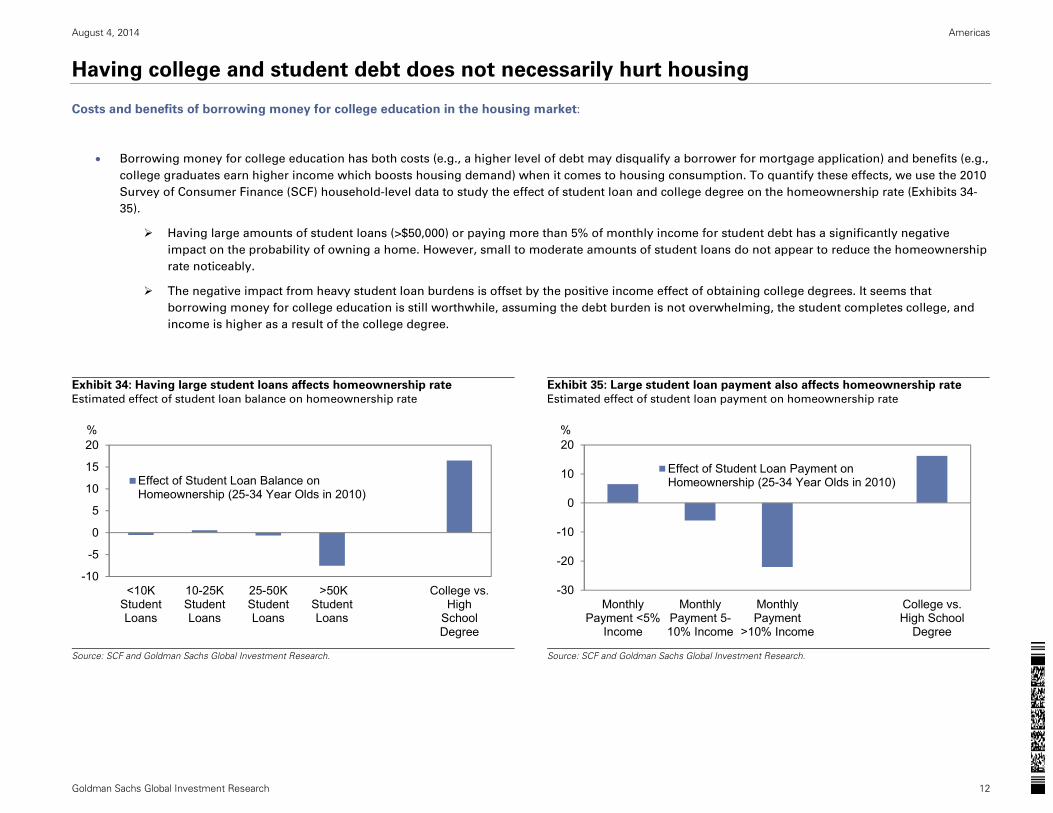
Having college and student debt does not necessarily hurt housing

Costs and benefits of borrowing money for college education in the housing market:

Borrowing money for college education has both costs (e.g., a higher level of debt may disqualify a borrower for mortgage application) and benefits (e.g.,

college graduates earn higher income which boosts housing demand) when it comes to housing consumption. To quantify these effects, we use the 2010

Survey of Consumer Finance (SCF) household-level data to study the effect of student loan and college degree on the homeownership rate (Exhibits 34-

35).

Having large amounts of student loans (>$50,000) or paying more than 5% of monthly income for student debt has a significantly negative

impact on the probability of owning a home. However, small to moderate amounts of student loans do not appear to reduce the homeownership

rate noticeably.

The negative impact from heavy student loan burdens is offset by the positive income effect of obtaining college degrees. It seems that

borrowing money for college education is still worthwhile, assuming the debt burden is not overwhelming, the student completes college, and

income is higher as a result of the college degree.

Exhibit 34: Having large student loans affects homeownership rate

Estimated effect of student loan balance on homeownership rate

Exhibit 35: Large student loan payment also affects homeownership rate

Estimated effect of student loan payment on homeownership rate



-10

-5

0

5

10

15

20

<10KStudentLoans

10-25KStudentLoans

25-50KStudentLoans

>50KStudentLoans

College vs.High

SchoolDegree

%

Effect of Student Loan Balance onHomeownership (25-34 Year Olds in 2010)

-30

-20

-10

0

10

20

MonthlyPayment <5%

Income

MonthlyPayment 5-10% Income

MonthlyPayment

>10% Income

College vs.High School

Degree

%

Effect of Student Loan Payment onHomeownership (25-34 Year Olds in 2010)



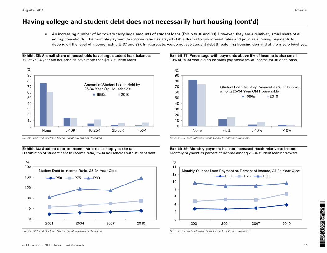
Having college and student debt does not necessarily hurt housing (cont’d)

An increasing number of borrowers carry large amounts of student loans (Exhibits 36 and 38). However, they are a relatively small share of all

young households. The monthly payment to income ratio has stayed stable thanks to low interest rates and policies allowing payments to

depend on the level of income (Exhibits 37 and 39). In aggregate, we do not see student debt threatening housing demand at the macro level yet.

Exhibit 36: A small share of households have large student loan balances 7% of 25-34 year old households have more than $50K student loans

Exhibit 37: Percentage with payments above 5% of income is also small 10% of 25-34 year old households pay above 5% of income for student loans



Exhibit 38: Student debt-to-income ratio rose sharply at the tail

Distribution of student debt to income ratio, 25-34 households with student debt

Exhibit 39: Monthly payment has not increased much relative to income

Monthly payment as percent of income among 25-34 student loan borrowers



0102030405060708090

None 0-10K 10-25K 25-50K >50K

%

1990s 2010

Amount of Student Loans Held by25-34 Year Old Households:

0102030405060708090

None <5% 5-10% >10%

%

1990s 2010

Student Loan Monthly Payment as % of Incomeamong 25-34 Year Old Households:

0

40

80

120

160

200

2001 2004 2007 2010

%

P50 P75 P90

Student Debt to Income Ratio, 25-34 Year Olds:

0

2

4

6

8

10

12

14

2001 2004 2007 2010

%

P50 P75 P90Monthly Student Loan Payment as Percent of Income, 25-34 Year Olds:



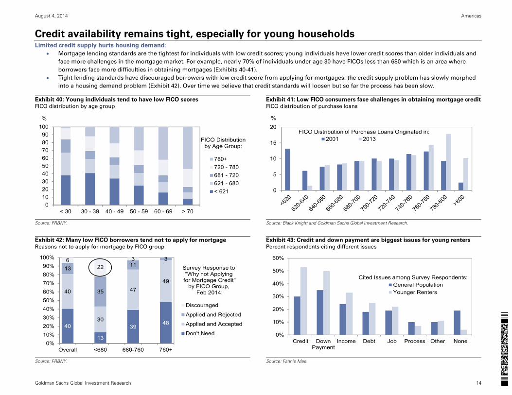
Credit availability remains tight, especially for young households Limited credit supply hurts housing demand:

Mortgage lending standards are the tightest for individuals with low credit scores; young individuals have lower credit scores than older individuals and

face more challenges in the mortgage market. For example, nearly 70% of individuals under age 30 have FICOs less than 680 which is an area where

borrowers face more difficulties in obtaining mortgages (Exhibits 40-41).

Tight lending standards have discouraged borrowers with low credit score from applying for mortgages: the credit supply problem has slowly morphed

into a housing demand problem (Exhibit 42). Over time we believe that credit standards will loosen but so far the process has been slow.

Exhibit 40: Young individuals tend to have low FICO scores FICO distribution by age group

Exhibit 41: Low FICO consumers face challenges in obtaining mortgage credit FICO distribution of purchase loans

Source: FRBNY.

Source: Black Knight and Goldman Sachs Global Investment Research.

Exhibit 42: Many low FICO borrowers tend not to apply for mortgage Reasons not to apply for mortgage by FICO group

Exhibit 43: Credit and down payment are biggest issues for young renters Percent respondents citing different issues

Source: FRBNY.

Source: Fannie Mae.

0102030405060708090

100

< 30 30 - 39 40 - 49 50 - 59 60 - 69 > 70

%

780+720 - 780681 - 720621 - 680< 621

FICO Distributionby Age Group:

0

5

10

15

20%

2001 2013FICO Distribution of Purchase Loans Originated in:

40

13

3948

40

30

4749

13

35

1136

223

0%10%20%30%40%50%60%70%80%90%

100%

Overall <680 680-760 760+

Discouraged

Applied and Rejected

Applied and Accepted

Don't Need

Survey Response to "Why not Applying

for Mortgage Credit"by FICO Group,

Feb 2014:

0%

10%

20%

30%

40%

50%

60%

Credit DownPayment

Income Debt Job Process Other None

General PopulationYounger Renters

Cited Issues among Survey Respondents:



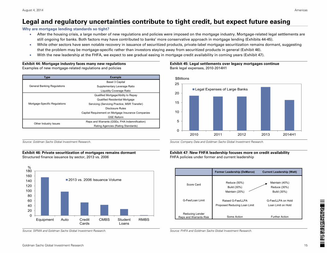
Legal and regulatory uncertainties contribute to tight credit, but expect future easing Why are mortgage lending standards so tight?

After the housing crisis, a large number of new regulations and policies were imposed on the mortgage industry. Mortgage-related legal settlements are

still ongoing for banks. Both factors may have contributed to banks’ more conservative approach in mortgage lending (Exhibits 44-45).

While other sectors have seen notable recovery in issuance of securitized products, private-label mortgage securitization remains dormant, suggesting

that the problem may be mortgage-specific rather than investors staying away from securitized products in general (Exhibit 46).

With the new leadership at the FHFA, we expect to see gradual easing in mortgage credit availability in coming years (Exhibit 47).

Exhibit 44: Mortgage industry faces many new regulations

Examples of new mortgage-related regulations and policies

Exhibit 45: Legal settlements over legacy mortgages continue

Bank legal expenses, 2010-2014H1


Source: Company Data and Goldman Sachs Global Investment Research.

Exhibit 46: Private securitization of mortgages remains dormant

Structured finance issuance by sector, 2013 vs. 2006

Exhibit 47: New FHFA leadership focuses more on credit availability

FHFA policies under former and current leadership

Source: SIFMA and Goldman Sachs Global Investment Research.

Source: FHFA and Goldman Sachs Global Investment Research.

Type Example

Basel 3 CapitalSupplementary Leverage Ratio

Liquidity Coverage RatioQualified Mortgage/Ability to Repay

Qualified Residential MortgageServicing (Servicing Practice, MSR Transfer)

Disclosure RulesCapital Requirement on Mortgage Insurance Companies

GSE ReformReps and Warrants (GSEs, FHA Indemnification)

Rating Agencies (Rating Standards)

General Banking Regulations

Mortgage-Specific Regulations

Other Industry Issues

0

5

10

15

20

25

2010 2011 2012 2013 2014H1

$Billions

Legal Expenses of Large Banks

020406080

100120140160180

Equipment Auto CreditCards

CMBS StudentLoans

RMBS

%

2013 vs. 2006 Issuance Volume

Former Leadership (DeMarco) Current Leadership (Watt)

Reduce (50%) Maintain (40%)Build (30%) Reduce (30%)

Maintain (20%) Build (30%)

Raised G-Fee/LLPA G-Fee/LLPA on HoldProposed Reducing Loan Limit Loan Limit on Hold

Reducing Lender Reps and Warrants Risk Some Action Further Action

Score Card

G-Fee/Loan Limit



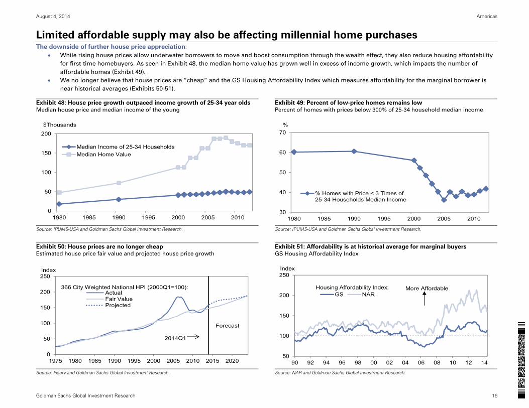
Limited affordable supply may also be affecting millennial home purchases The downside of further house price appreciation:

While rising house prices allow underwater borrowers to move and boost consumption through the wealth effect, they also reduce housing affordability

for first-time homebuyers. As seen in Exhibit 48, the median home value has grown well in excess of income growth, which impacts the number of

affordable homes (Exhibit 49).

We no longer believe that house prices are “cheap” and the GS Housing Affordability Index which measures affordability for the marginal borrower is

near historical averages (Exhibits 50-51).

Exhibit 48: House price growth outpaced income growth of 25-34 year olds

Median house price and median income of the young

Exhibit 49: Percent of low-price homes remains low

Percent of homes with prices below 300% of 25-34 household median income



Exhibit 50: House prices are no longer cheap Estimated house price fair value and projected house price growth

Exhibit 51: Affordability is at historical average for marginal buyers

GS Housing Affordability Index

Source: Fiserv and Goldman Sachs Global Investment Research.

Source: NAR and Goldman Sachs Global Investment Research.

0

50

100

150

200

1980 1985 1990 1995 2000 2005 2010

$Thousands

Median Income of 25-34 HouseholdsMedian Home Value

30

40

50

60

70

1980 1985 1990 1995 2000 2005 2010

%

% Homes with Price < 3 Times of25-34 Households Median Income

0

50

100

150

200

250

1975 1980 1985 1990 1995 2000 2005 2010 2015 2020

Index

ActualFair ValueProjected

366 City Weighted National HPI (2000Q1=100):

2014Q1

Forecast

50

100

150

200

250

90 92 94 96 98 00 02 04 06 08 10 12 14

Index

GS NARHousing Affordability Index: More Affordable



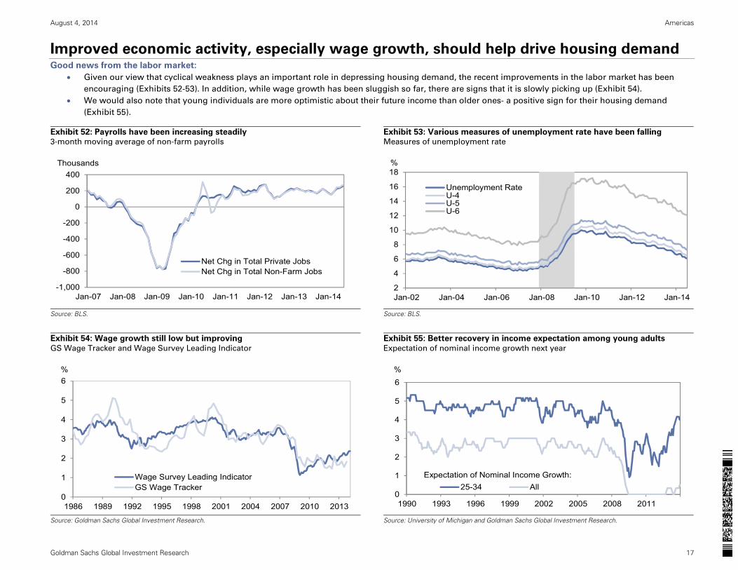
Improved economic activity, especially wage growth, should help drive housing demand Good news from the labor market:

Given our view that cyclical weakness plays an important role in depressing housing demand, the recent improvements in the labor market has been

encouraging (Exhibits 52-53). In addition, while wage growth has been sluggish so far, there are signs that it is slowly picking up (Exhibit 54).

We would also note that young individuals are more optimistic about their future income than older ones- a positive sign for their housing demand

(Exhibit 55).

Exhibit 52: Payrolls have been increasing steadily 3-month moving average of non-farm payrolls

Exhibit 53: Various measures of unemployment rate have been falling Measures of unemployment rate

Source: BLS.

Source: BLS.

Exhibit 54: Wage growth still low but improving

GS Wage Tracker and Wage Survey Leading Indicator

Exhibit 55: Better recovery in income expectation among young adults

Expectation of nominal income growth next year


Source: University of Michigan and Goldman Sachs Global Investment Research.

-1,000

-800

-600

-400

-200

0

200

400

Jan-07 Jan-08 Jan-09 Jan-10 Jan-11 Jan-12 Jan-13 Jan-14

Thousands

Net Chg in Total Private JobsNet Chg in Total Non-Farm Jobs

2

4

6

8

10

12

14

16

18

Jan-02 Jan-04 Jan-06 Jan-08 Jan-10 Jan-12 Jan-14

%

Unemployment RateU-4U-5U-6

0

1

2

3

4

5

6

1986 1989 1992 1995 1998 2001 2004 2007 2010 2013

%

Wage Survey Leading IndicatorGS Wage Tracker

0

1

2

3

4

5

6

1990 1993 1996 1999 2002 2005 2008 2011

%

25-34 AllExpectation of Nominal Income Growth:



Scenario analysis suggests recovery continues even in “stress test” scenario

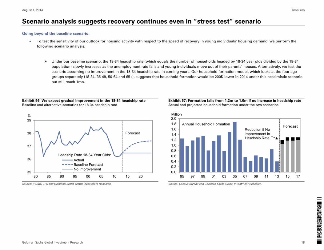
Going beyond the baseline scenario:

To test the sensitivity of our outlook for housing activity with respect to the speed of recovery in young individuals’ housing demand, we perform the

following scenario analysis.

Under our baseline scenario, the 18-34 headship rate (which equals the number of households headed by 18-34 year olds divided by the 18-34

population) slowly increases as the unemployment rate falls and young individuals move out of their parents’ houses. Alternatively, we test the

scenario assuming no improvement in the 18-34 headship rate in coming years. Our household formation model, which looks at the four age

groups separately (18-34, 35-49, 50-64 and 65+), suggests that household formation would be 200K lower in 2014 under this pessimistic scenario

but still reach 1mn.

Exhibit 56: We expect gradual improvement in the 18-34 headship rate Baseline and alternative scenarios for 18-34 headship rate

Exhibit 57: Formation falls from 1.2m to 1.0m if no increase in headship rateActual and projected household formation under the two scenarios


Source: Census Bureau and Goldman Sachs Global Investment Research.

35

36

37

38

39

80 85 90 95 00 05 10 15 20

%

ActualBaseline ForecastNo Improvement

Forecast

Headship Rate 18-34 Year Olds:

0.00.20.40.60.81.01.21.41.61.82.0

95 97 99 01 03 05 07 09 11 13 15 17

Million

Annual Household Formation ForecastReduction if No Improvement in Headship Rate



Scenario analysis suggests recovery continues even in “stress test” scenario (cont’d)

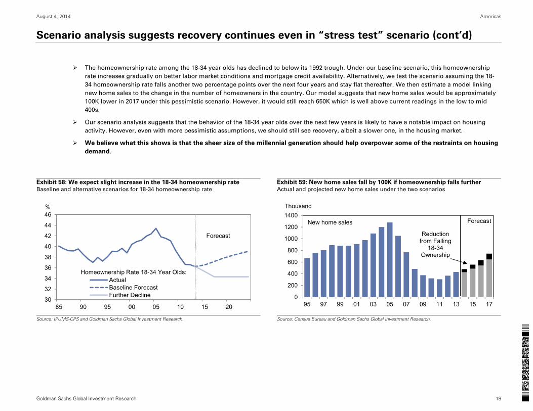
The homeownership rate among the 18-34 year olds has declined to below its 1992 trough. Under our baseline scenario, this homeownership

rate increases gradually on better labor market conditions and mortgage credit availability. Alternatively, we test the scenario assuming the 18-

34 homeownership rate falls another two percentage points over the next four years and stay flat thereafter. We then estimate a model linking

new home sales to the change in the number of homeowners in the country. Our model suggests that new home sales would be approximately

100K lower in 2017 under this pessimistic scenario. However, it would still reach 650K which is well above current readings in the low to mid

400s.

Our scenario analysis suggests that the behavior of the 18-34 year olds over the next few years is likely to have a notable impact on housing

activity. However, even with more pessimistic assumptions, we should still see recovery, albeit a slower one, in the housing market.

We believe what this shows is that the sheer size of the millennial generation should help overpower some of the restraints on housing

demand.

Exhibit 58: We expect slight increase in the 18-34 homeownership rate

Baseline and alternative scenarios for 18-34 homeownership rate

Exhibit 59: New home sales fall by 100K if homeownership falls further

Actual and projected new home sales under the two scenarios


Source: Census Bureau and Goldman Sachs Global Investment Research.

30

32

34

36

38

40

42

44

46

85 90 95 00 05 10 15 20

%

ActualBaseline ForecastFurther Decline

Forecast

Homeownership Rate 18-34 Year Olds:

0

200

400

600

800

1000

1200

1400

95 97 99 01 03 05 07 09 11 13 15 17

Thousand

New home sales

Reduction from Falling

18-34Ownership

Forecast



Taking a hard look at what young adults can buy today

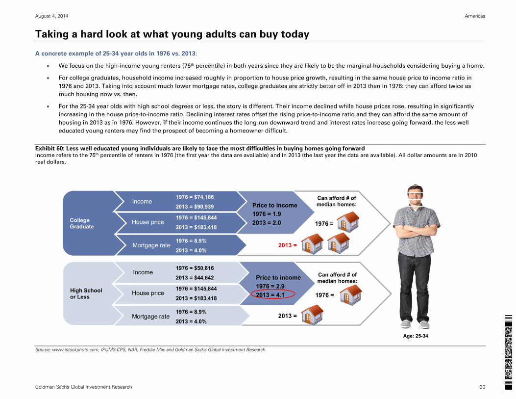
A concrete example of 25-34 year olds in 1976 vs. 2013:

We focus on the high-income young renters (75th percentile) in both years since they are likely to be the marginal households considering buying a home.

For college graduates, household income increased roughly in proportion to house price growth, resulting in the same house price to income ratio in

1976 and 2013. Taking into account much lower mortgage rates, college graduates are strictly better off in 2013 than in 1976: they can afford twice as

much housing now vs. then.

For the 25-34 year olds with high school degrees or less, the story is different. Their income declined while house prices rose, resulting in significantly

increasing in the house price-to-income ratio. Declining interest rates offset the rising price-to-income ratio and they can afford the same amount of

housing in 2013 as in 1976. However, if their income continues the long-run downward trend and interest rates increase going forward, the less well

educated young renters may find the prospect of becoming a homeowner difficult.

Exhibit 60: Less well educated young individuals are likely to face the most difficulties in buying homes going forward Income refers to the 75th percentile of renters in 1976 (the first year the data are available) and in 2013 (the last year the data are available). All dollar amounts are in 2010

real dollars.

Source: www.istockphoto.com, IPUMS-CPS, NAR, Freddie Mac and Goldman Sachs Global Investment Research.

Age: 25-34

√

Price to income1976 = 2.92013 = 4.1

Price to income1976 = 1.92013 = 2.0

High School or Less

College Graduate

Income

Mortgage rate

House price

Income

House price

Mortgage rate

1976 = $50,816

2013 = $44,642

1976 = $145,844

2013 = $183,418

1976 = 8.9%

2013 = 4.0%

1976 = $74,186

2013 = $90,939

1976 = $145,844

2013 = $183,418

1976 = 8.9%

2013 = 4.0%

Can afford # of median homes:

Can afford # of median homes:

2013 =

1976 =

2013 =

1976 =



Where does it leave us? Expect growth in housing demand but restraints hold us back

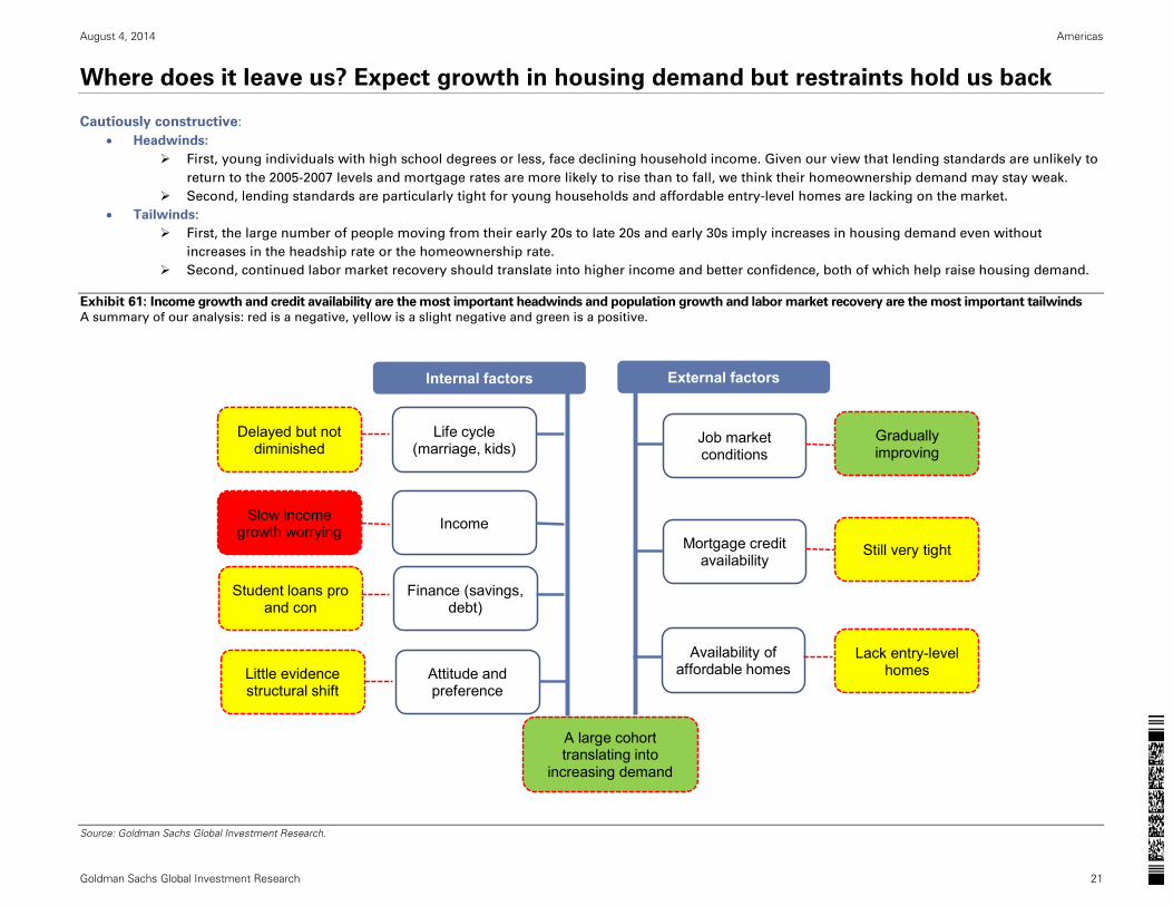
Cautiously constructive:

Headwinds:

First, young individuals with high school degrees or less, face declining household income. Given our view that lending standards are unlikely to

return to the 2005-2007 levels and mortgage rates are more likely to rise than to fall, we think their homeownership demand may stay weak.

Second, lending standards are particularly tight for young households and affordable entry-level homes are lacking on the market.

Tailwinds:

First, the large number of people moving from their early 20s to late 20s and early 30s imply increases in housing demand even without

increases in the headship rate or the homeownership rate.

Second, continued labor market recovery should translate into higher income and better confidence, both of which help raise housing demand.

Exhibit 61: Income growth and credit availability are the most important headwinds and population growth and labor market recovery are the most important tailwinds A summary of our analysis: red is a negative, yellow is a slight negative and green is a positive.


Internal factors

Life cycle (marriage, kids)

Income

Finance (savings, debt)

Attitude and preference

Delayed but notdiminished

Slow income growth worrying

Student loans pro and con

Little evidence structural shift

External factors

Job market conditions

Mortgage credit availability

Availability of affordable homes

Gradually improving

Still very tight

Lack entry-level homes

A large cohort translating into

increasing demand



Disclosure Appendix

Reg AC

We, Eli Hackel, CFA and Hui Shan, hereby certify that all of the views expressed in this report accurately reflect our personal views about the subject company or companies and its or their securities.

We also certify that no part of our compensation was, is or will be, directly or indirectly, related to the specific recommendations or views expressed in this report.

Investment Profile

The Goldman Sachs Investment Profile provides investment context for a security by comparing key attributes of that security to its peer group and market. The four key attributes depicted are: growth,

returns, multiple and volatility. Growth, returns and multiple are indexed based on composites of several methodologies to determine the stocks percentile ranking within the region's coverage

universe.

The precise calculation of each metric may vary depending on the fiscal year, industry and region but the standard approach is as follows:

Growth is a composite of next year's estimate over current year's estimate, e.g. EPS, EBITDA, Revenue. Return is a year one prospective aggregate of various return on capital measures, e.g. CROCI,

ROACE, and ROE. Multiple is a composite of one-year forward valuation ratios, e.g. P/E, dividend yield, EV/FCF, EV/EBITDA, EV/DACF, Price/Book. Volatility is measured as trailing twelve-month

volatility adjusted for dividends.

Quantum

Quantum is Goldman Sachs' proprietary database providing access to detailed financial statement histories, forecasts and ratios. It can be used for in-depth analysis of a single company, or to make

comparisons between companies in different sectors and markets.

GS SUSTAIN

GS SUSTAIN is a global investment strategy aimed at long-term, long-only performance with a low turnover of ideas. The GS SUSTAIN focus list includes leaders our analysis shows to be well

positioned to deliver long term outperformance through sustained competitive advantage and superior returns on capital relative to their global industry peers. Leaders are identified based on

quantifiable analysis of three aspects of corporate performance: cash return on cash invested, industry positioning and management quality (the effectiveness of companies' management of the

environmental, social and governance issues facing their industry).

Disclosures

Coverage group(s) of stocks by primary analyst(s)

Eli Hackel, CFA: America-Building Products, America-Homebuilders.

America-Building Products: Armstrong World Industries, Inc., Fortune Brands Home & Security, Inc., Masco Corporation, Mohawk Industries, Inc., Owens Corning, Ply Gem Holdings, Inc., USG

Corporation.

America-Homebuilders: Beazer Homes USA, Inc., D.R. Horton, Inc., Hovnanian Enterprises, Inc., KB Home, Lennar Corp., M.D.C. Holdings, Inc., Meritage Homes Corp., NVR, Inc., PulteGroup, Inc.,

Realogy Holdings Corp, Taylor Morrison Home Corp., The Ryland Group, Inc., Toll Brothers, Inc..

Distribution of ratings/investment banking relationships

Goldman Sachs Investment Research global coverage universe

Rating Distribution Investment Banking Relationships

Buy Hold Sell Buy Hold Sell

Global 32% 54% 14% 42% 36% 30%

As of July 1, 2014, Goldman Sachs Global Investment Research had investment ratings on 3,697 equity securities. Goldman Sachs assigns stocks as Buys and Sells on various regional Investment

Lists; stocks not so assigned are deemed Neutral. Such assignments equate to Buy, Hold and Sell for the purposes of the above disclosure required by NASD/NYSE rules. See 'Ratings, Coverage

groups and views and related definitions' below.

Regulatory disclosures

Disclosures required by United States laws and regulations

See company-specific regulatory disclosures above for any of the following disclosures required as to companies referred to in this report: manager or co-manager in a pending transaction; 1% or

other ownership; compensation for certain services; types of client relationships; managed/co-managed public offerings in prior periods; directorships; for equity securities, market making and/or

specialist role. Goldman Sachs usually makes a market in fixed income securities of issuers discussed in this report and usually deals as a principal in these securities.



The following are additional required disclosures: Ownership and material conflicts of interest: Goldman Sachs policy prohibits its analysts, professionals reporting to analysts and members of their

households from owning securities of any company in the analyst's area of coverage. Analyst compensation: Analysts are paid in part based on the profitability of Goldman Sachs, which includes

investment banking revenues. Analyst as officer or director: Goldman Sachs policy prohibits its analysts, persons reporting to analysts or members of their households from serving as an officer,

director, advisory board member or employee of any company in the analyst's area of coverage. Non-U.S. Analysts: Non-U.S. analysts may not be associated persons of Goldman, Sachs & Co. and

therefore may not be subject to NASD Rule 2711/NYSE Rules 472 restrictions on communications with subject company, public appearances and trading securities held by the analysts.

Distribution of ratings: See the distribution of ratings disclosure above. Price chart: See the price chart, with changes of ratings and price targets in prior periods, above, or, if electronic format or if

with respect to multiple companies which are the subject of this report, on the Goldman Sachs website at http://www.gs.com/research/hedge.html.

Additional disclosures required under the laws and regulations of jurisdictions other than the United States

The following disclosures are those required by the jurisdiction indicated, except to the extent already made above pursuant to United States laws and regulations. Australia: Goldman Sachs Australia

Pty Ltd and its affiliates are not authorised deposit-taking institutions (as that term is defined in the Banking Act 1959 (Cth)) in Australia and do not provide banking services, nor carry on a banking

business, in Australia. This research, and any access to it, is intended only for "wholesale clients" within the meaning of the Australian Corporations Act, unless otherwise agreed by Goldman Sachs. In

producing research reports, members of the Global Investment Research Division of Goldman Sachs Australia may attend site visits and other meetings hosted by the issuers the subject of its research

reports. In some instances the costs of such site visits or meetings may be met in part or in whole by the issuers concerned if Goldman Sachs Australia considers it is appropriate and reasonable in the

specific circumstances relating to the site visit or meeting. Brazil: Disclosure information in relation to CVM Instruction 483 is available at http://www.gs.com/worldwide/brazil/area/gir/index.html.

Where applicable, the Brazil-registered analyst primarily responsible for the content of this research report, as defined in Article 16 of CVM Instruction 483, is the first author named at the beginning of

this report, unless indicated otherwise at the end of the text. Canada: Goldman Sachs Canada Inc. is an affiliate of The Goldman Sachs Group Inc. and therefore is included in the company specific

disclosures relating to Goldman Sachs (as defined above). Goldman Sachs Canada Inc. has approved of, and agreed to take responsibility for, this research report in Canada if and to the extent that

Goldman Sachs Canada Inc. disseminates this research report to its clients. Hong Kong: Further information on the securities of covered companies referred to in this research may be obtained on

request from Goldman Sachs (Asia) L.L.C. India: Further information on the subject company or companies referred to in this research may be obtained from Goldman Sachs (India) Securities Private

Limited. Japan: See below. Korea: Further information on the subject company or companies referred to in this research may be obtained from Goldman Sachs (Asia) L.L.C., Seoul Branch. New Zealand: Goldman Sachs New Zealand Limited and its affiliates are neither "registered banks" nor "deposit takers" (as defined in the Reserve Bank of New Zealand Act 1989) in New Zealand. This

research, and any access to it, is intended for "wholesale clients" (as defined in the Financial Advisers Act 2008) unless otherwise agreed by Goldman Sachs. Russia: Research reports distributed in the

Russian Federation are not advertising as defined in the Russian legislation, but are information and analysis not having product promotion as their main purpose and do not provide appraisal within

the meaning of the Russian legislation on appraisal activity. Singapore: Further information on the covered companies referred to in this research may be obtained from Goldman Sachs (Singapore)

Pte. (Company Number: 198602165W). Taiwan: This material is for reference only and must not be reprinted without permission. Investors should carefully consider their own investment risk.

Investment results are the responsibility of the individual investor. United Kingdom: Persons who would be categorized as retail clients in the United Kingdom, as such term is defined in the rules of

the Financial Conduct Authority, should read this research in conjunction with prior Goldman Sachs research on the covered companies referred to herein and should refer to the risk warnings that

have been sent to them by Goldman Sachs International. A copy of these risks warnings, and a glossary of certain financial terms used in this report, are available from Goldman Sachs International

on request.

European Union: Disclosure information in relation to Article 4 (1) (d) and Article 6 (2) of the European Commission Directive 2003/126/EC is available at

http://www.gs.com/disclosures/europeanpolicy.html which states the European Policy for Managing Conflicts of Interest in Connection with Investment Research.

Japan: Goldman Sachs Japan Co., Ltd. is a Financial Instrument Dealer registered with the Kanto Financial Bureau under registration number Kinsho 69, and a member of Japan Securities Dealers

Association, Financial Futures Association of Japan and Type II Financial Instruments Firms Association. Sales and purchase of equities are subject to commission pre-determined with clients plus

consumption tax. See company-specific disclosures as to any applicable disclosures required by Japanese stock exchanges, the Japanese Securities Dealers Association or the Japanese Securities

Finance Company.

Ratings, coverage groups and views and related definitions

Buy (B), Neutral (N), Sell (S) -Analysts recommend stocks as Buys or Sells for inclusion on various regional Investment Lists. Being assigned a Buy or Sell on an Investment List is determined by a

stock's return potential relative to its coverage group as described below. Any stock not assigned as a Buy or a Sell on an Investment List is deemed Neutral. Each regional Investment Review

Committee manages various regional Investment Lists to a global guideline of 25%-35% of stocks as Buy and 10%-15% of stocks as Sell; however, the distribution of Buys and Sells in any particular

coverage group may vary as determined by the regional Investment Review Committee. Regional Conviction Buy and Sell lists represent investment recommendations focused on either the size of the

potential return or the likelihood of the realization of the return.

Return potential represents the price differential between the current share price and the price target expected during the time horizon associated with the price target. Price targets are required for all

covered stocks. The return potential, price target and associated time horizon are stated in each report adding or reiterating an Investment List membership.

Coverage groups and views: A list of all stocks in each coverage group is available by primary analyst, stock and coverage group at http://www.gs.com/research/hedge.html. The analyst assigns one

of the following coverage views which represents the analyst's investment outlook on the coverage group relative to the group's historical fundamentals and/or valuation. Attractive (A). The

investment outlook over the following 12 months is favorable relative to the coverage group's historical fundamentals and/or valuation. Neutral (N). The investment outlook over the following 12

months is neutral relative to the coverage group's historical fundamentals and/or valuation. Cautious (C). The investment outlook over the following 12 months is unfavorable relative to the coverage

group's historical fundamentals and/or valuation.

Not Rated (NR). The investment rating and target price have been removed pursuant to Goldman Sachs policy when Goldman Sachs is acting in an advisory capacity in a merger or strategic

transaction involving this company and in certain other circumstances. Rating Suspended (RS). Goldman Sachs Research has suspended the investment rating and price target for this stock, because

there is not a sufficient fundamental basis for determining, or there are legal, regulatory or policy constraints around publishing, an investment rating or target. The previous investment rating and

price target, if any, are no longer in effect for this stock and should not be relied upon. Coverage Suspended (CS). Goldman Sachs has suspended coverage of this company. Not



Covered (NC). Goldman Sachs does not cover this company. Not Available or Not Applicable (NA). The information is not available for display or is not applicable. Not Meaningful (NM). The

information is not meaningful and is therefore excluded.

Global product; distributing entities

The Global Investment Research Division of Goldman Sachs produces and distributes research products for clients of Goldman Sachs on a global basis. Analysts based in Goldman Sachs offices

around the world produce equity research on industries and companies, and research on macroeconomics, currencies, commodities and portfolio strategy. This research is disseminated in Australia

by Goldman Sachs Australia Pty Ltd (ABN 21 006 797 897); in Brazil by Goldman Sachs do Brasil Corretora de Títulos e Valores Mobiliários S.A.; in Canada by either Goldman Sachs Canada Inc. or

Goldman, Sachs & Co.; in Hong Kong by Goldman Sachs (Asia) L.L.C.; in India by Goldman Sachs (India) Securities Private Ltd.; in Japan by Goldman Sachs Japan Co., Ltd.; in the Republic of Korea by

Goldman Sachs (Asia) L.L.C., Seoul Branch; in New Zealand by Goldman Sachs New Zealand Limited; in Russia by OOO Goldman Sachs; in Singapore by Goldman Sachs (Singapore) Pte. (Company

Number: 198602165W); and in the United States of America by Goldman, Sachs & Co. Goldman Sachs International has approved this research in connection with its distribution in the United

Kingdom and European Union.

European Union: Goldman Sachs International authorised by the Prudential Regulation Authority and regulated by the Financial Conduct Authority and the Prudential Regulation Authority, has

approved this research in connection with its distribution in the European Union and United Kingdom; Goldman Sachs AG and Goldman Sachs International Zweigniederlassung Frankfurt, regulated

by the Bundesanstalt für Finanzdienstleistungsaufsicht, may also distribute research in Germany.

General disclosures

This research is for our clients only. Other than disclosures relating to Goldman Sachs, this research is based on current public information that we consider reliable, but we do not represent it is

accurate or complete, and it should not be relied on as such. We seek to update our research as appropriate, but various regulations may prevent us from doing so. Other than certain industry reports

published on a periodic basis, the large majority of reports are published at irregular intervals as appropriate in the analyst's judgment.

Goldman Sachs conducts a global full-service, integrated investment banking, investment management, and brokerage business. We have investment banking and other business relationships with a

substantial percentage of the companies covered by our Global Investment Research Division. Goldman, Sachs & Co., the United States broker dealer, is a member of SIPC (http://www.sipc.org).

Our salespeople, traders, and other professionals may provide oral or written market commentary or trading strategies to our clients and our proprietary trading desks that reflect opinions that are

contrary to the opinions expressed in this research. Our asset management area, our proprietary trading desks and investing businesses may make investment decisions that are inconsistent with the

recommendations or views expressed in this research.

The analysts named in this report may have from time to time discussed with our clients, including Goldman Sachs salespersons and traders, or may discuss in this report, trading strategies that

reference catalysts or events that may have a near-term impact on the market price of the equity securities discussed in this report, which impact may be directionally counter to the analyst's published

price target expectations for such stocks. Any such trading strategies are distinct from and do not affect the analyst's fundamental equity rating for such stocks, which rating reflects a stock's return

potential relative to its coverage group as described herein.

We and our affiliates, officers, directors, and employees, excluding equity and credit analysts, will from time to time have long or short positions in, act as principal in, and buy or sell, the securities or

derivatives, if any, referred to in this research.

The views attributed to third party presenters at Goldman Sachs arranged conferences, including individuals from other parts of Goldman Sachs, do not necessarily reflect those of Global Investment

Research and are not an official view of Goldman Sachs.

Any third party referenced herein, including any salespeople, traders and other professionals or members of their household, may have positions in the products mentioned that are inconsistent with

the views expressed by analysts named in this report.

This research is not an offer to sell or the solicitation of an offer to buy any security in any jurisdiction where such an offer or solicitation would be illegal. It does not constitute a personal

recommendation or take into account the particular investment objectives, financial situations, or needs of individual clients. Clients should consider whether any advice or recommendation in this

research is suitable for their particular circumstances and, if appropriate, seek professional advice, including tax advice. The price and value of investments referred to in this research and the income

from them may fluctuate. Past performance is not a guide to future performance, future returns are not guaranteed, and a loss of original capital may occur. Fluctuations in exchange rates could have

adverse effects on the value or price of, or income derived from, certain investments.

Certain transactions, including those involving futures, options, and other derivatives, give rise to substantial risk and are not suitable for all investors. Investors should review current options

disclosure documents which are available from Goldman Sachs sales representatives or at http://www.theocc.com/about/publications/character-risks.jsp. Transaction costs may be significant in option

strategies calling for multiple purchase and sales of options such as spreads. Supporting documentation will be supplied upon request.

All research reports are disseminated and available to all clients simultaneously through electronic publication to our internal client websites. Not all research content is redistributed to our clients or

available to third-party aggregators, nor is Goldman Sachs responsible for the redistribution of our research by third party aggregators. For research, models or other data available on a particular

security, please contact your sales representative or go to http://360.gs.com.

Disclosure information is also available at http://www.gs.com/research/hedge.html or from Research Compliance, 200 West Street, New York, NY 10282.

© 2014 Goldman Sachs.

No part of this material may be (i) copied, photocopied or duplicated in any form by any means or (ii) redistributed without the prior written consent of The Goldman Sachs Group, Inc.

millennials: the housing edition

Documents