mimicking short-term memory in shape- reconstruction task ... using fuzzy t2.pdf · abstract— the...
TRANSCRIPT
Page 1 of 29
Abstract— The paper attempts to model short-term memory (STM) for shape-reconstruction tasks by
employing a 4-stage deep brain leaning network (DBLN), where the first 2 stages are built with Hebbian
learning and the last 2 stages with Type-2 Fuzzy logic. The model is trained stage-wise independently with
visual stimulus of the object-geometry as the input of the first stage, EEG acquired from different cortical
regions as input and output of respective intermediate stages, and recalled object-geometry as the output of
the last stage. Two error feedback loops are employed to train the proposed DBLN. The inner loop adapts the
weights of the STM based on a measure of error in model-predicted response with respect to the object-shape
recalled by the subject. The outer loop adapts the weights of the iconic (visual) memory based on a measure of
error of the model predicted response with respect to the desired object-shape. In the test phase, the DBLN
model reproduces the recalled object shape from the given input object geometry.
The motivation of the paper is to test the consistency in STM encoding (in terms of similarity in network
weights) for repeated visual stimulation with the same geometric object. Experiments undertaken on healthy
subjects, yield high similarity in network weights, whereas patients with pre-frontal lobe Amnesia yield
significant discrepancy in the trained weights for any two trials with the same training object. This justifies
the importance of the proposed DBLN model in automated diagnosis of patients with learning difficulty. The
novelty of the paper lies in the overall design of the DBLN model with special emphasis to the last 2 stages of
the network, built with vertical slice based type-2 fuzzy logic, to handle uncertainty in function approximation
(with noisy EEG data). The proposed technique outperforms the state-of-the-art functional mapping
algorithms with respect to the (pre-defined outer loop) error metric, computational complexity and runtime.
Index Terms— Short-term memory, iconic memory, Hebbian learning, type-2 fuzzy set, shape reconstruction,
memory failure and N400.
I. INTRODUCTION
The human memory is distributed across the brain with functionally pronounced active regions located in the medial
temporal lobe, called Hippocampus, for use as the Long-Term Memory (LTM) and the pre-frontal lobe for use as the
Short-Term Memory (STM) [1-5]. Although very little of the encoding and recall processes of human memory
system is known till this date [6-7], strong evidences of having two distinct cortical pathways for STM and LTM
recalls for visuo-spatial object-recognition tasks exist in the literature [8-11]. While for the STM-recall, the occipito-
parietal pathway [8-9] is primarily responsible, the occipito-temporal pathway is used for the LTM-recall [10-11].
Neuro-physiological support of the above evidences also is reported in quite a few interesting scientific treaties [12-
16]. The current research on cognitive neuroscience further reveals that the STM encoding and recall for object-shape
recognition task is performed in the Gamma frequency band (30-100 Hz) [8], [17-19]. There also exist evidences of
related brain activities, including visual perception and object recognition in the Gamma band [2], [20-21].
The paper aims at developing one computational model of the STM for use in the shape-reconstruction task with
the motivation to determine the degradation in recall-performance of the memory using electroencephalographic
(EEG) signatures of the selected brain lobes. Unfortunately, the memory models [22-29] available in the current
literature are mostly philosophical in nature, with minimal scope of use for diagnostic and therapeutic applications.
Although traces of STM analysis using EEG signal exist in the literature [30-44], there is a void of research on STM
modeling using EEG. This void has inspired the present research group to model STM using EEG signatures. As the
encoding and the recall pathways of memory involve other brain modules, modeling of memory independently is not
Mimicking Short-Term Memory in Shape-
Reconstruction Task Using an EEG-Induced
Type-2 Fuzzy Deep Brain Learning Network
Lidia Ghosh, Amit Konar, Pratyusha Rakshit, and Atulya K. Nagar

Page 2 of 29
easy. In fact, memory modeling requires an integrated approach with a mission to study the stimulus-response pairs
of the relevant brain modules lying on the encoding and the recall pathways [8-11].
EEG provides an interesting means to detect old/new-effect [74] of memory by utilizing one well-known brain
signal, called N400 [73]. The N400 signal exhibits a negative peak in response to new (unknown) visual input
stimulus. It is usually observed that the negativity of N400 gradually diminishes, as the subject becomes more
familiar with the object [74]. This particular characteristic of N400 signal is used here to determine the STM
performance in 2-dimensional object shape-reconstruction task.
Deep Learning (DL) [54] is currently gaining increasing interest from diverse research community for its efficient
performance in classification [87-89] and functional mapping [90-91] problems from raw data. Deep learning
algorithms differ from conventional neural network algorithms for having exceedingly large number of layers to
extract high level features/attributes from low level raw data. For example, in Convolutional Neural Net (CNN) [68]
based Deep Learning, the motivation is to extract features of objects from a large pool of object-dataset. In CNN,
during the recall phase, layers occupying the later stages offer more refined object features than the preceding layers.
Generally, extracts of the penultimate layer often are regarded as object-features, while the last layer provides the
class information in a multi-class classification problem.
Although conventional deep learning algorithms aim at imitating the behavioral mechanism of learning in the
brain [92-93], they hardly realize the cognitive functionalities of the individual brain modules [95] involved in the
learning process. This paper makes an honest attempt to synthesize functionality of different brain modules by
distinctive layers with suitable non-linearity in the context of STM encoding and recall. It introduces a novel
technique of STM-modeling in the settings of deep brain learning, where the individual brain functions involved in
STM encoding and recall cycles are modeled by developing the functional mapping from the input to the output.
During the STM encoding and recall phases (of the shape-reconstruction experiments), four distinct functional
mappings are extracted from the EEG signals acquired from the occipital, pre-frontal and parietal lobes. The first
functional mapping is developed from the input visual stimuli and the occipital EEG response to the stimuli. The
second functional mapping refers to the interdependence between the EEG signals acquired from the occipital and
the pre-frontal lobes during the shape-encoding phase. This mapping is useful to predict pre-frontal response from the
occipital response in the recall cycle later. The third mapping refers to pre-frontal to parietal mapping, resembling the
functionality of the parietal lobe. This mapping helps in determining the parietal response, if the pre-frontal response
is known during the recall phase. The last mapping between the parietal responses to the geometric features of the
reconstructed (hand-drawn) object-shape indicates the parietal and motor cortex behavior jointly.
Machine learning models have successfully been used in Brain-Computer Interfaces (BCI) to handle two
fundamental problems: i) classification of brain signals for different cognitive activities/malfunctioning [52], [82-84]
and ii) synthesis of the functional mapping of the active brain lobes from their measured input-output [77]. This
paper aims at serving the second problem. Although the functional mapping can be realized by a number of ways,
here the mapping of the first 2-stages is realized by Hebbian learning [45], while that of the third and the fourth
stages is designed by Type-2 Fuzzy logic. The choice of Hebbian learning appears from the fundamental basis of
Hebb’s principle of an excited neuron’s natural tendency to stimulate a neighborhood neuron [46-48]. The Hebbian
learning, being unsupervised, fits well for signal transduction at low level (early stage of) neural processing [81]. On
Actual object
geometry
Input object geometry to
Iconic Memory mapping
realized with feed-forward
neural network
Iconic Memory to STM
mapping realized with
feed-forward neural
network
STM to parietal
lobe mapping
realized with
T2FS
Parietal lobe to hand-
drawn object
geometry mapping
realized with T2FS
Input
object
geometry
Model-
produced object
geometry
Iconic memory
response STM
response
Parietal lobe
response
+ -
STM weight
adaptation using Perceptron-Like
learning
Hand-drawn object
geometry
+ -
Iconic memory
weight adaptation
using Perceptron-
Like learning
Change in Iconic
Memory
weight
Change in STM
weight
Fig. 1.(a) General Block-diagram of the proposed DBLN describing 4-stage functional mapping with feedback for STM and Iconic Memory weight
adaptation

Page 3 of 29
the other hand, at higher level (later stage of) neural signal transduction [60], supervised learning is employed to
quantize the neural signals to converge to fixed points, representing object classes in the recognition problem, and the
desired output level in the functional mapping problems. Further, due to asynchronous firing of neurons in different
brain lobes, noise is introduced in the signaling pathways, causing undesirable changes in the outputs. The advent of
fuzzy sets, in particular its type-2 counterpart has immense potential in approximate reasoning, which is expected to
play a vital role in the neural quantization process in presence of noise [77]. Thus type-2 fuzzy logic is expected to
serve well in functional mapping at higher level neural learning.
Two distinct varieties of type-2 fuzzy sets are widely being used in the literature [50-53], [65-66]. They are well-
known as Interval Type-2 Fuzzy Sets (IT2FS) [50] and General Type-2 Fuzzy Sets (GT2FS) [51]. In classical fuzzy
sets, the membership function of a linguistic variable lying in [0,1] is crisp, whereas in type-2 fuzzy set, the
corresponding (primary) membership is fuzzy, as the linguistic variable at a given linguistic value has a wide range
of primary membership in [0,1]. GT2FS fundamentally differs from IT2FS with respect to secondary (type-2)
Membership Function (MF). In GT2FS, the secondary membership function takes any value in [0, 1], whereas in
IT2FS the secondary membership function is considered 1 for all feasible primary memberships lying within a
region, referred to as Footprint of Uncertainty (FOU), and is zero elsewhere. Because of its representational
advantages, GT2FS can capture higher degrees of uncertainty [52], however at the cost of additional computational
overhead. Here, a special type of GT2FS, called vertical slice [53], is used to design a novel algorithm for functional
mapping between pre-frontal to parietal lobe and parietal lobe to hand-drawn object-geometry.
The paper is divided into seven sections. Section II provides the system overview. In Section III, principles and
methodology are covered in brief. Section-IV deals with experiments and results. Biological implications of the
experimental results are summarized in Section V. Performance analysis by statistical tests is undertaken in Section
VI. Conclusions are listed in Section VII.
II. SYSTEM OVERVIEW
This section provides an overview of the proposed type-2 fuzzy deep brain learning network (DBLN), containing
four stages of functional mapping, shown in Fig. 1 (a). The input-output layers of each functional mapping module
are explicitly indicated in Fig. 1(b). The geometric features of an object, to be reconstructed, are assigned at the first
Fig. 1.(b) The Model used in 4-stage mapping of the DBLN, explicitly showing the input and the output features of each module
Iconic memory
response
(Occipital EEG
features)
STM response (Pre-
frontal
EEG features)
W G
Pre-trained
T2FS1
Pre-trained T2FS2
Iconic Memory Weight Adaptation
+
-
Original object
shape
Input
Shape
Parietal EEG
features Iconic Memory
Model
STM Model
a1
a2
a3
a4
a5
a6
W
+ -
G
.
.
.
.
.
.
c1
c2
c3
c16
b1
b2
b3
b4
b5
b6
d1
d2
d3
d4
d5
d6
c'1
c'2
c'3
c'16
.
.
.
.
.
.
If E>1 , then adapt
ijiaEg ..
,
Object geometric
features
Model-produced Object
geometric features
If ,2
E then adapt
lilcEw .. '
,
Reproduced
object shape at the end
of each learning epoch
][
lc
16
1
' )(l
ll ccE
][l
c
][l
c
)ˆ(16
1
l
ll ccE
Model produced
object shape
][l
c
STM Weight Adaptation

Page 4 of 29
(input) layer of the proposed feed-forward network architecture (Fig. 1(b)). These features are obtained from the gray
scale image of the object by the following steps: i) Gaussian filtering with user defined standard deviation to smooth
the raw gray scale image, ii) Edge detection and thinning by non-maximal suppression [85], here realized with Canny
edge detection [85], iii) Line parameters (perpendicular distance of the line from the origin, , and the angle
between the above perpendicular line with the x-axis) detection by Hough Transform [86], iv) Evaluation of line end
point coordinates, line length and adjacent sides of the polygon having common vertices and v) computation of the
angle between each two adjacent lines. The steps are illustrated in the Appendix. The length of the straight line edges
and angles between adjacent edges are used as the geometric features of the object.
The weight matrixnpil
w
2,
][W between the first and the second layers represents the weighted connectivity
between the geometric feature lc of the visually perceived object and the iconic memory response ai, where p denotes
the number of vertices of the perceived object, and n denotes the number of electrodes placed on the occipital lobe
(Fig. 1(b)). The second layer (the first hidden layer), thus contains the iconic memory response. The weight matrix
nnjig ][ ,G between the second and the third layers represents the connectivity weights between the iconic memory
response ai and STM response ,jb where i, j{1, n}(Fig. 1(b)). The third (the second hidden) layer thus contains STM
response ,jb j = 1 to n.
The parietal lobe used for smart movement-related planning is modeled here by type-2 fuzzy logic for its inherent
benefit of approximate reasoning (here, functional mapping) in presence of noisy input/output training samples. In
absence of fuzzy functional mapping, noise present in the training samples acquired from the EEG electrodes, might
result in unexpected changes in function approximation. Let }1:{ njbj
and }1:{ nkdk
be the one dimensional
EEG features (average Gamma power) extracted from the pre-frontal and the parietal lobes respectively during the
STM recall phase of the shape-recognition task. The functional mapping: b1, b2, …,bn dk for all k is developed
using type-2 Fuzzy sets. Thus the fourth (the third hidden) layer embedded in the DBLN takes care of noisy EEG
data acquired from the parietal lobe response dk, k = 1 to n. The parietal lobe response to geometric features of the
recalled/reconstructed hand-drawn object is represented here by one additional module of type-2 fuzzy reasoning.
The choice of fuzzy mapping here too is ascertained to avoid possible creeping of noise in the mapping function. The
last (output) layer, thus, contains the geometric features lc of the reconstructed object.
The following 3 issues need special mention while undertaking training of the proposed feed-forward architecture.
1. First, each stage of the proposed functional mapping is trained independently with acquired input and output
instances of the corresponding layer. The input instance of the first layer is obtained from the object geometry, while
the same for other layers is obtained from EEG data. The output instance of all excluding the last layer is obtained
from EEG data, while that of the last layer is obtained from subject-produced drawing of the recalled object.
2. The training instances of the first two stages of functional mapping are obtained from the EEG signals acquired
during the phase of memory encoding. On the other hand, the training instances of the last 2 stages are generated
from the acquired EEG, during the memory recall phase of the subject.
3. After the training of 4 individual stages of mapping is over, two error feedback loops are employed in the model,
where the inner loop adapts the weights of the short-term memory based on a measure of error in model-predicted
response with respect to object-shape recalled/drawn by the subject. The outer loop adapts the weights of the iconic
(visual) memory based on a measure of error of the model predicted response with respect to the desired object-
shape.
It is important to mention here that during the encoding of iconic memory and the STM, the subject observes a 2-
dimensional planer object of asymmetric shape (with linear boundaries) for 10 seconds with an intension to
remember the 2-dimensional geometry of the object for subsequent participation in the memory recall phase. On the
other hand, during the memory recall phase, the subject recollects the 2-D planar object from his/her memory and
draws the object on a piece of paper. A brief overview of the layer-wise training of individual stages of Fig. 1 is
given below.
1. For iconic memory encoding, the geometric features of the object (extracted by Hough transform) and average
Gamma power [20] of the EEG signals acquired from the occipital lobe are used as the input and output respectively
Page 5 of 29
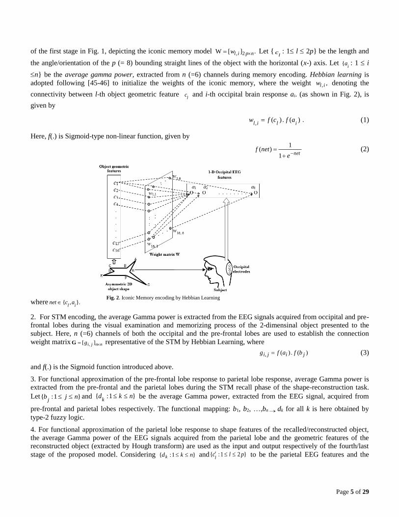
of the first stage in Fig. 1, depicting the iconic memory model , 2W [ ] .l i p nw Let {l
c : 1 l 2p} be the length and
the angle/orientation of the p (= 8) bounding straight lines of the object with the horizontal (x-) axis. Let i
a{ : 1 i
n} be the average gamma power, extracted from n (=6) channels during memory encoding. Hebbian learning is
adopted following [45-46] to initialize the weights of the iconic memory, where the weight , ,l iw denoting the
connectivity between l-th object geometric feature lc and i-th occipital brain response ai. (as shown in Fig. 2), is
given by
.)(.)(, ilil
afcfw (1)
Here, f(.) is Sigmoid-type non-linear function, given by
netenetf
1
1)( (2)
where }.,{il
acnet
2. For STM encoding, the average Gamma power is extracted from the EEG signals acquired from occipital and pre-
frontal lobes during the visual examination and memorizing process of the 2-dimensinal object presented to the
subject. Here, n (=6) channels of both the occipital and the pre-frontal lobes are used to establish the connection
weight matrix nnjig ][ ,G representative of the STM by Hebbian Learning, where
)(.)(, jiji bfafg (3)
and f(.) is the Sigmoid function introduced above.
3. For functional approximation of the pre-frontal lobe response to parietal lobe response, average Gamma power is
extracted from the pre-frontal and the parietal lobes during the STM recall phase of the shape-reconstruction task.
Let }1:{ njbj
and }1:{ nkdk
be the average Gamma power, extracted from the EEG signal, acquired from
pre-frontal and parietal lobes respectively. The functional mapping: b1, b2, …,bn dk for all k is here obtained by
type-2 fuzzy logic.
4. For functional approximation of the parietal lobe response to shape features of the recalled/reconstructed object,
the average Gamma power of the EEG signals acquired from the parietal lobe and the geometric features of the
reconstructed object (extracted by Hough transform) are used as the input and output respectively of the fourth/last
stage of the proposed model. Considering }1:{ nkdk and }21:{ plcl
to be the parietal EEG features and the
Fig. 2. Iconic Memory encoding by Hebbian Learning

Page 6 of 29
parameters of the drawn object respectively, a type-2 fuzzy mapping is employed to obtain the required mapping: d1,
d2, …, dnl
c for all l.
The training phase of the proposed DBLN system (Fig. 1) constitutes two fundamental steps: i) encoding of W
and G matrices along with construction of functional mappings: b1, b2, …, bn dk and d1, d2, …, dn lc for all k
and l, and ii) adaptation of W and G matrices by supervised learning. Here, W and G matrices are first encoded using
Hebbian learning. The functional mappings indicated above are constructed using type-2 fuzzy sets and the
adaptation of W and G matrices are performed using Perceptron-like learning equation [46].
III. BRAIN FUNCTIONAL MAPPING USING TYPE-2 FUZZY DBLN
Principles of brain functional mapping introduced in Section II is realized here using type-2 fuzzy DBLN with
feedback loops realized with Perceptron-like learning equation. The section has 5 parts. In Section A, a brief
overview of IT2FS and GT2FS is given. Section B introduces the realization of functional mappings of i) prefrontal
to parietal lobe and ii) parietal lobe to object-shape-geometry by a novel type-2 fuzzy vertical slice approach. In
Section C, the weight adaptation of W and G matrices is carried out by perceptron-like learning. The training and
testing of the proposed fuzzy neural architecture are presented in Section D and E respectively.
A. Overview of Type-2 Fuzzy Sets
Definition 1: A type-1(T1)/classical fuzzy set A [49] is an ordered pairs of a linguistic variable x and its membership
value ( )A x in A, given by
{( , ( )) | }AA x x x X (4)
where, X is the universe of discourse. Usually, )(xA is a crisp number, lying in [0, 1] for any .Xx
Definition 2: A General Type-2 Fuzzy Set A~
is given by ]},1,0[,|)),(),,{((~
~ uXxuxuxAA
where x is a linguistic
variable defined on a universe of discourse X, u [0,1] is the primary membership and ( , )A
x u is a secondary MF,
given by the mapping ( , )A
x u where ( , )A
x u too lies in [0, 1] [51], [76].
Definition 3: For a given value of x, say ,xx the 2D plane comprising u and ( )( )
A xu is called a vertical slice of
the GT2FS [53].
Definition 4: An Interval Type-2 Fuzzy Set (IT2FS) [51] is a special form of GT2FS with ),(~ uxA
= 1, for x X and
u[0, 1]. A closed IT2FS (CIT2FS) is one form of IT2FS where { [0,1] | ( , ) 1}x AI u x u is a closed interval for
every x X [76]. Here, CIT2FS is used throughout the paper. All IT2FS mentioned in this paper are CIT2FS.
However, they are referred to as IT2FS as done in most of the literature [76].
Definition 5: The Footprint of Uncertainty (FOU) of a type-2 Fuzzy set (T2FS) A~
is defined as the union of all its
primary memberships [76]. The mathematical representation of FOU is
Xx
xJA
)~
(FOU (5)
where, }.0),(],1,0[|),{( ~ uxuuxJAx FOU is a bounded region, which represents the uncertainty in the primary
memberships of the T2FS.
Definition 6: An embedded fuzzy set Ae(x) is an arbitrarily selected type-1 MF lying in the FOU,
i.e., .,)( XxJxAxe
Definition 7: The embedded fuzzy set, representing the upper bound of FOU( A~
) is called the upper membership
function (UMF) and it is denoted by FOU( )A (or ( ))A
x , Xx [76]. Similarly, the embedded fuzzy set, representing
the lower bound of FOU( A~
), is called the lower membership function (LMF) and is denoted as FOU( )A (or ( ))A
x ,
Xx . More precisely,

Page 7 of 29
):)(()~
(FOU)()~
(UMF ~ XxxAMaxAxAeA
(6)
and ):)(()~
(FOU)()~
(LMF ~ XxxAMinAxAeA
(7)
B. Type-2 Fuzzy Mapping and Parameter Adaptation by Perceptron-like Learning
This section attempts to construct the functional mappings for i)prefrontal to parietal and ii) parietal to object-shape
geometry using the acquired EEG signals from the selected brain lobes. The EEG signals acquired are usually found
to be contaminated with stochastic noise due to non-voluntary motor actions like eye-blinking and artifacts due to
simultaneous brain activation for concurrent thoughts [58]. Very often the noise and the desired brain signals have
overlapped frequency spectra, thereby making filtering algorithms inefficient for the targeted application. Naturally,
the superimposed stochastic noise yields erroneous results in mapping, if realized with classical mapping techniques,
such as neural functional approximation [55-56], nonlinear regression [57] and the like. Fuzzy logic has shown
promising performance in functional mapping in presence of noisy measurements because of their inherent
nonlinearity in the MFs (Gaussian/Triangular) [78]. The effect of measurement noise in functional mapping is
reduced further in T2FS [77] because of its characteristic to handle intra-personal level uncertainty due to the
presence of stochastic noise. These works inspired the authors to realize the brain mapping functions using IT2FS
and one vertical slice approach [53] of GT2FS. In addition to type-2 fuzzy mapping, parameter adaptation of the
mapping function is also needed to attain optimal performance.
B.1 Construction of the Proposed Interval Type-2 Fuzzy Membership Function (IT2MF): Let U and V be the 2 brain
signals, acquired from two distinct brain lobes, during the memory recall phase. Considering a time-duration of 30
seconds for drawing the object from the STM, and a sampling rate of EEG = 5000 samples/second, the total number
of EEG samples acquired from each brain region = 5000 × 30 = 1,50,000. These total number of samples (i.e.,
1,50,000 samples), obtained over the duration of 30 seconds, are divided into 30 time-slots of equal length of 5000
samples each. The Power Spectral Density (PSD) in gamma frequency band (30-100 Hz) is then extracted for each
time slot. The PSD over a slot is then described by a Gaussian MF: Ԍ (μ, σ2) with μ and σ2 representing the mean and
variance of the PSD of 5000 samples over the slot. The MF: ),(xiA where Ai = Close-to-center of the support [49] of
the MF and x = PSD, represents that power is close to mean value of the PSD over 5000 samples. Thus for 30 time-
slots, 30 type-1 Gaussian MFs: A1, A2, …,A30 are obtained. The following 2 steps are performed to construct the
IT2FS (Fig. 3(b)) [ ( ), ( )]AA
A x x from the 30 type-1 Gaussian MFs.
xxxxMinx AAAA )],(...,),(),([)(
3021~ (8)
xxxxMaxx AAAA )],(...,),(),([)(
3021~ (9)
where, ( )A
x and ( )A
x respectively denote the LMF and the UMF of the said IT2FS x is .A In order to maintain the
convexity criterion [59] of IT2FS, the peaks of the Type-1 MFs are joined with a straight line of zero slope, resulting
in a flat-top approximated IT2FS (see Fig. 3(c)).
B.2 Construction of IT2FS induced Mapping Function: To design the mapping function between 2 brain lobes, the
EEG signal is acquired from both the lobes simultaneously during a learning epoch. Let ),(1 tx ),(2 tx …, )(txn and
),(1 ty ),(2 ty …, )(tyn be the gamma power extracted from n electrodes of a source lobe and n electrodes of a
destination lobe respectively during the learning epoch. The IT2MFs ix is iA~
for i = 1 to n and jy is ,~
jB for j = 1 to
n (see Fig. 4) are obtained by the technique introduced in section B.1.
Fig. 3. Computation of flat-top IT2FS: (a) type-1 MFs, (b) IT2FS
representation of the type-1 MFs, (c) Flat-topped IT2FS
)(~ iiA
x
ix ix
1 1
)(~ iiA
x
ix
)(~ iiA
x
UMF
LMF
1
LMF
UMF
(a) (b) (c)

Page 8 of 29
Now let ii xx for i = 1 to n be a sample measurement (here, average Gamma power). To map ,11 xx ,22 xx
…, nn xx to ,jj
yy the following transformation is used.
)(t...t)(t)( ~22
~11
~ nnAAA
xxxSUF (10)
)(t...t)(t)( ~22
~11
~ nnAAA
xxxSLF (11)
where, )(~ ijA
x and )(~ ijA
x are the upper membership function (UMF) and lower membership function (LMF) of
)(~ iiA
x at .ii
xx In (10) and (11), the t-norms [49] are computed sequentially in order of their appearance from
the left to the right. To control the area under the IT2FS ,~
jB the following transformations are used.
, for 1 to .j jUFS UFS j n (12)
.to1for, n jSLFLFS jj (13)
Here, jUFS and jLFS are the firing strength of the selected rule, and j and j are two control parameters used to
adapt the area under the consequent membership function (MF) jy is .~
jB The IT2 inference is obtained as
jjjBjj
jByyUFSy
),()( ~~ (14)
and .),()( ~~jj
jBjjjB
yyLFSy
(15)
The IT2FS consequent ,~
jB represented by )](),([ ~~j
jBjjB
yy is next defuzzified by a proposed Average (Av.)
Defuzzification Algorithm to obtain the centroid C, given by
.~ofUMFtheofSupport
~consequenttheofArea
j
j
B
BC
(16)
),( 1~1,
uxjA
Av. Defuzzification
Fig. 4. Adaptation of the IT2FS induced mapping function by Perceptron-like learning
1x 1x
),(,
~ uxnA nj
... ...
j
t-norm SUF
t-norm SLF
)(~ jjB
y
/ ( )jB jy
jUFS
jLFS
y
nx nx
j
IT2 inference
generation
C
j
jy
Perceptron-like
Learning
If ,0j
.| | . ;j j UFS j j j
.| | . ;jjLFS jjj
If ,0j
;.. SUFjj
jjj
;.. SLFjj
jjj
- +
jy

Page 9 of 29
Let, .Cy j Also, let jy be the desired value. The following steps are used next to adapt the control parameters
j and j to control the area under the FOU of the inference.
Let, ,jjj
yy (17)
For ,0j
| | , where ,
| | , where ,j j j j j
jj j j j
UFS
LFS
(18)
For ,0j
, where ,
, where ,j j j j j
jj j j j
UFS
LFS
(19)
where 0 1. The adaptation of j
and j is done in the training phase. After the training with known ]...,,,[21 n
xxx
and ]...,,,[ 21 nyyy vectors is over, the weights j
and j are fixed forever and may directly be used in the test
phase.
)()1(1,
~ uxjA
u
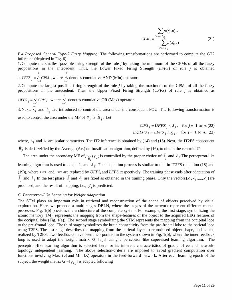
Fig. 6. GT2FS based mapping adapted with Perceptron-like learning
Cumulative OR operation
i
n
ij CPMUFFS
1
j
… … …
… ..
)()(,
~ unxnjA
1x
u
… …
j
j
u
nx
0
u
jLFFS
jUFFS
1x
n
x
/ ( )jB jy
jLFS
jUFS
( )jB
y
y
Computation of CPM1 Computation of CPMn
… …
Cumulative AND operation
i
n
ij CPMLFFS
1
Perceptron-like
Learning
jy
- +
jy
( )jB
y
If ,0j
.| | . ;j j jUFFS j j j
.| | . ;j jjLFFS jjj
If ,0j
;..jjj
UFFS jjj
;..jjj
LFFS jjj
Av. Defuzzification
C
IT2 inference
generation
0

Page 10 of 29
B.3 Secondary Membership Function Computation of
Proposed GT2FS: Consider the rule: If 1x is 1
~A and 2x is
2~A and … and nx is
nA~ Then jy is .
~jB Here, ix is iA
~for
i= 1 to n are GT2FS-induced propositions and jy is jB~
denotes an IT2FS consequent MF. Here, the secondary MFs
with respect to the primary memberships at given ii xx of the GT2FS proposition are represented by a vertical slice
[53]. Let )()(
~ uixiA
be the secondary MF for the ith antecedent proposition ix is .~
iA Given the measurements ii xx
for i = 1 to n, the vertical planes representing secondary memberships )()(
~ uixiA
at ii xx are identified. Let the
primary membership u at ii xx is spatially sampled as u1, u2, …, um. Given the contributory primary memberships,
which jointly comprise the FOU, the secondary MF at a given value of the linguistic variable ii xx is computed
using the following steps.
1. Divide the interval [0, ]mu at ii xx into equal sized intervals ,u such that each interval contains at least one type-
1 primary membership (see Fig. 5).
2. Count the number of primary memberships that cross the intervals ,011 uu ,122 uuu …,
1 mmm uuu at .ii xx Let 1 2, ,..., mv v v be the respective counts for the intervals ....,,, 21 muuu
3. Obtain the secondary MF at the mid-points of the intervals:21
rr
uu
by using (20) for r =1 to m.
}to1:{Max21)(~
mrv
vuu
r
rrr
ixA
(20)
This is illustrated in Fig. 5, where the numbers of type-1 memberships that cross the intervals 654
and, uuu for
instances at ixix respectively are 1, 3 and 4. Therefore, ,25.04
1
2
43)(
~
uu
ixA
75.0
4
3
2
54)(
~
uu
ixA
and
.14
4
2
65)(
~
uu
ixA
4. Compute the centroid of the vertical slice by using the centre of gravity method and declare it as the contribution
of the primary membership (CPM) of the fuzzy proposition: i
x is ,~iA in the firing strength computation of the rule.
The CPMi for i
x is Aiis obtained as
1
Fig. 5. Secondary Membership Assignment in the proposed GT2FS based
mapping technique
)()(,
~ uixijA
ix
u
ix
2u
3u
4u
6u
5u
6u
1u
1
0
Page 11 of 29
ix
ix
Ju
i
Ju
i
iux
uux
CPM),(
).,(
(21)
B.4 Proposed General Type-2 Fuzzy Mapping: The following transformations are performed to compute the GT2
inference (depicted in Fig. 6):
1. Compute the smallest possible firing strength of the rule j by taking the minimum of the CPMs of all the fuzzy
propositions in the antecedent. Thus, the Lower Fixed Firing Strength (LFFS) of rule j is obtained
as ,1
i
n
ij CPMLFFS
where
n
i 1 denotes cumulative AND (Min) operator.
2. Compute the largest possible firing strength of the rule j by taking the maximum of the CPMs of all the fuzzy
propositions in the antecedent. Thus, the Upper Fixed Firing Strength (UFFS) of rule j is obtained as
,1
i
n
ij CPMUFFS
where
n
i 1 denotes cumulative OR (Max) operator.
3. Next, j and j are introduced to control the area under the consequent FOU. The following transformation is
used to control the area under the MF of jy is .
~j
B Let
.to1for, n jUFFSUFS jjj (22)
and .to1for, n jLFFSLFS jjj (23)
where, j and j are scalar parameters. The IT2 inference is obtained by (14) and (15). Next, the IT2FS consequent
jB ~
is de-fuzzified by the Average (Av.) de-fuzzification algorithm, defined by (16), to obtain the centroid C.
The area under the secondary MF of )('~ jjB
y is controlled by the proper choice of j
and .j The perceptron-like
learning algorithm is used to adapt j
and .j The adaptation process is similar to that in IT2FS (equation (18) and
(19)), where SUF and SLF are replaced by UFFSj and LFFSj respectively. The training phase ends after adaptation of
j and .j In the test phase,
j and j
are fixed as obtained in the training phase. Only the vectors ]....,,,[21 n
xxx are
produced, and the result of mapping, i.e., j
y is predicted.
C. Perceptron-Like Learning for Weight Adaptation
The STM plays an important role in retrieval and reconstruction of the shape of objects perceived by visual
exploration. Here, we propose a multi-stages DBLN, where the stages of the network represent different mental
processes. Fig. 1(b) provides the architecture of the complete system. For example, the first stage, symbolizing the
iconic memory (IM), represents the mapping from the shape-features of the object to the acquired EEG features of
the occipital lobe (Fig. 1(a)). The second stage symbolizing the STM represents the mapping from the occipital lobe
to the pre-frontal lobe. The third stage symbolizes the brain connectivity from the pre-frontal lobe to the parietal lobe
using T2FS. The last stage describes the mapping from the parietal layer to reproduced object shape, and is also
realized by T2FS. Two feedbacks have been incorporated in the system shown in Fig. 1(b), where the inner feedback
loop is used to adapt the weight matrix ][ , jigG using a perceptron-like supervised learning algorithm. The
perceptron-like learning algorithm is selected here for its inherent characteristics of gradient-free and network-
topology independent learning. The above selection-criteria are imposed to avoid gradient computation over
functions involving Max ( ) and Min () operators in the feed-forward network. After each learning epoch of the
subject, the weight matrix G = ][, ji
g is adapted following
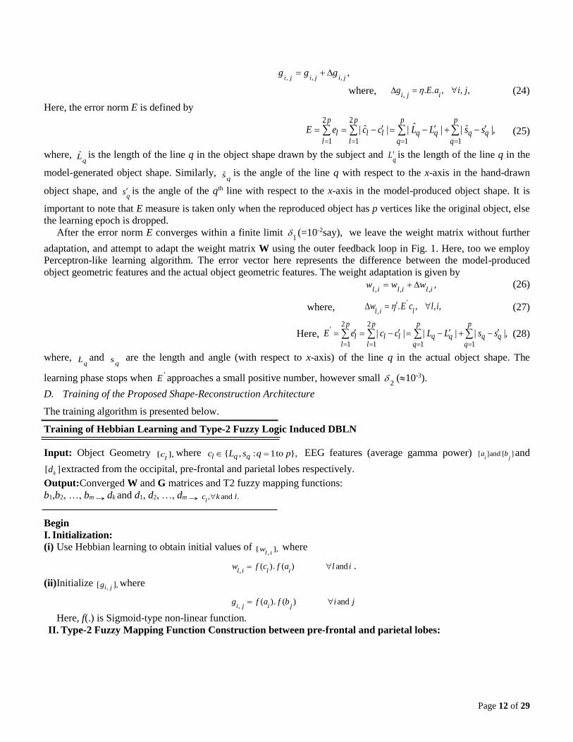
Page 12 of 29
,,,, jijiji
ggg
where, ,,,..,
jiaEgiji
(24)
Here, the error norm E is defined by
|,ˆ||ˆ||ˆ|11
2
1
2
1q
p
qqq
p
p
lll
p
ll ssLLcceE
(25)
where, q
L is the length of the line q in the object shape drawn by the subject and q
L is the length of the line q in the
model-generated object shape. Similarly, q
s is the angle of the line q with respect to the x-axis in the hand-drawn
object shape, and q
s is the angle of the qth line with respect to the x-axis in the model-produced object shape. It is
important to note that E measure is taken only when the reproduced object has p vertices like the original object, else
the learning epoch is dropped.
After the error norm E converges within a finite limit 1
(=10-2say), we leave the weight matrix without further
adaptation, and attempt to adapt the weight matrix W using the outer feedback loop in Fig. 1. Here, too we employ
Perceptron-like learning algorithm. The error vector here represents the difference between the model-produced
object geometric features and the actual object geometric features. The weight adaptation is given by
,,,, ililil
www (26)
where, ,,,. '
,ilcEw
lil (27)
Here, |,|||||11
2
1
2
1
'q
p
qqq
p
p
lll
p
ll ssLLcceE
(28)
where, q
L and q
s are the length and angle (with respect to x-axis) of the line q in the actual object shape. The
learning phase stops when 'E approaches a small positive number, however small 2
(10-3).
D. Training of the Proposed Shape-Reconstruction Architecture
The training algorithm is presented below.
Training of Hebbian Learning and Type-2 Fuzzy Logic Induced DBLN
Input: Object Geometry ],[l
c where { , : 1to },l q qc L s q p EEG features (average gamma power) ][and][ji
ba and
[ ]kd extracted from the occipital, pre-frontal and parietal lobes respectively.
Output:Converged W and G matrices and T2 fuzzy mapping functions:
b1,b2, …, bm dk and d1, d2, …, dm .and, lkcl
Begin
I. Initialization:
(i) Use Hebbian learning to obtain initial values of ],[, il
w where
ilafcfwilil
and)(.)(,
.
(ii) Initialize ,[ ],i jg where
jibfafgjiji
and)(.)(,
Here, f(.) is Sigmoid-type non-linear function.
II. Type-2 Fuzzy Mapping Function Construction between pre-frontal and parietal lobes:

Page 13 of 29
Construct IT2/GT2 mapping function b1,b2, …,bm dk for k to realize pre-frontal to parietal functional
connectivity. Given kd as the target feature, compare error ,kkk dd and adapt parameters k and k using (18)-
(19) until k andk are less than predefined real value (=10-2).
III.Type-2 Fuzzy Mapping Function Construction between parietal lobe features and reproduced object
shape geometric features:
Construct IT2/GT2 mapping function d1, d2, …,dn lcl, for to realize parietal to reproduced object shape
geometry functional connectivity. Given l
c as the target feature, compare l by (17) and adapt parameters l and
l using (18)-(19), until l and l are less than predefined real value (=10-2).
IV. G matrix Adaptation:
This step involves a) computation of ,l
c b) Computation of error E, and c) adaptation of G matrix using the error E.
Let ]ˆ[l
c and ][l
c be the geometric features of the reproduced and model-produced object geometric features
respectively.
a) Compute l
c by the following steps.
i) Compute iconic memory response i
a from the object-shape parameters l
c for l= 1 to 2p by the following
transformations:
(1 ) 1 2 2[ ] [ ] . ,i n l p ( p n)a c W
.to1for)( niafaii
ii) Compute Pre-frontal response ,j
b j = 1 to n, by the following transformations:
(1 ) 1[ ] [ ] . ,( )
Gj n i n n nb a
.to1for)( njbfbjj
iii) Compute parietal response k
d for k = 1 to m from the computed prefrontal response by IT2/GT2 fuzzy
mapping, introduced in section III.
iv) Compute predicted object-shape parameter l
c for l=1 to 2p by IT2/GT2 fuzzy mapping, introduced in section
III.
a) Compute error lll
cce ˆ for l= 1 to 2p.
b) Use Perceptron-like learning algorithm to adjust weights ji
g,
by the following steps.
i) .,,..,
jiaEgiji
ii) .,,,,,
jigggjijiji
iii) Repeat from step (i) until ,1E for some small positive real number .
1
Here, the sign of E determines the increase/decrease in ij
g as desired.
V) W-matrix Adaptation
Let [ ]lc and [ ]lc be the geometric features of the original and model-produced object geometric features respectively.
Compute l l le c c and use perceptron-like learning given by ,. '
, lilcEw for all l and i. The sign of 'E determines
increase/decrease in il
w,
as desired. Continue il
w,
adaptation until 'E is less than a predefined threshold δ2.
b) Return npil
w
2,
][W ,l i and ,[ ]G i j n ng , .i j
End.

Page 14 of 29
To confirm that the brain response obtained is due to neurons participating as memory, the negativity of N400 [73] is
checked after each learning epoch. It is important to mention here that the decreasing negativity of N400 is observed
with increasing learning epochs for the same training object. Details of N400 signal processing is available in [61].
E. The Test Phase of the Memory Model
Once the training phase is over, the network may be used for reproduction of the model-generated object shape for a
given input object shape. Here, the geometric features [cl] for l= 1 to 2p for integer p, and the converged W matrix,
G matrix and pre-constructed Type-2 Mapping function are used as input of the algorithm. The algorithm returns
computed geometric features [ ]lc of the object presented to the subject for visual inspection. The steps (i) to (iv) under
step IV.a) of the training algorithm are executed to obtain [ ]lc from [cl] for l= 1 to 2p.
IV. EXPERIMENTS AND RESULTS
A. Experimental Set-up
A 21-channel EEG system manufactured by Nihon Kohden has been employed for the present experiments. Here,
earlobe electrodes A1 and A2 are used as the reference and the Fpz electrode as the ground. Further, 6 electrodes are
selected from each of the occipital, pre-frontal and the parietal lobes to test the mapping of EEG features from the
occipital to the pre-frontal lobe during STM encoding and later from the pre-frontal to the parietal lobes during the
memory recall phase. The 10-20 electrode placement [62] (Fig. 7) is used in the present experimental set-ups, and the
PSD in the gamma band (30-100 Hz), called gamma power [20], is used as the feature for each channel. All
experiments are performed using MATLAB-16b toolbox running under Windows-10 operating system on Intel
Octacore processor with clock speed 2 GHz and RAM 64 GB.
Fig. 7. 10-20 electrode placement system (only the blue circled
electrodes are used for the present experiment)
Fig. 8. Stimulus preparation
First Trial
+ IM
Encoding STM
Encoding
10s 2s
STM
Recall
STM to
Parietal
Mapping
Parietal to Desired
Object Shape
Mapping
Error norm
(E and E’)
Computation
50s 50s
STM
Encoding STM
Recall
Second Trial
Error norm
(E and E’)
Computation
10s
Rest
60s
Repeated Trials
+ STM
Encoding
50s 10s
STM
Recall
2s 2s
+ Error norm
(E and E’)
Computation

Page 15 of 29
Experiments are undertaken on 35 subjects in the age group 20-30 years. 30 of the 35 members are healthy, while
the remaining 5 are suffering from memory impairment (2 suffering from temporal lobe epilepsy and 3 suffering
from Alzheimer’s disease with pre-frontal lobe amnesia). Each subject is advised to take a comfortable resting
position with arms on the armrest to avoid possible pick-ups of muscle artifacts. During the encoding phase, objects
of asymmetric shapes, similar to the one shown in Fig. 1, are used as visual stimuli for the STM of the subject. The
subject is advised to remember the object-shape, presented to him/her as a visual stimulus for 10 seconds (Fig. 8).
The EEG signals are acquired from the occipital and the pre-frontal lobes at the end of this 10 seconds interval. Next,
during the recall phase, the subject is asked to draw the object-shape from his STM. EEG is then acquired from all
the electrodes, and common average referencing [80] is performed to eliminate the artifacts due to hand movements
in drawing. In order to examine the effect of repeated STM learning, the same visual stimulus is presented after a
time-delay of 60 seconds (Fig. 8). The STM learning is repeated -times ( ≥1) until the learnt object shape matches
with the sample object. The steps narrated above are performed repeatedly for 10 different asymmetric object shapes
(as shown in Fig. 9), for each of the 35 subjects. The object shapes are presented in the Fig. 9 with increasing shape
complexity.
B. Experiment 1 (Validation of the STM model with respect to error metric ξ)
The motivation of this experiment is to compare the model-produced G matrices over successive trials with the same
object-shape on the same subject. An error metric ξ is introduced to measure the relative difference between the G
matrices of successive trials, where ξ is computed by
,),(
||
,,
,,
i j jiji
jiji
ggMax
gg (29)
where, jig , and jig , are the STM weights obtained from two successive learning trials. The reproduced object-shape
after each trial and the corresponding error metric are given in Table-I for one healthy subject S3 with the best STM
performance.
TABLE I. VALIDATION OF THE STM MODEL WITH RESPECT TO ξFOR 2 OBJECTS
Original
2D object
shape
Reproduced object shapes with the
evaluated
Trial 1 Trial 2 Trial 3
( = 3.91)
( = 1.91) ( =
0.13)
( = 2.62)
( = 1.18)
( =
0.02)
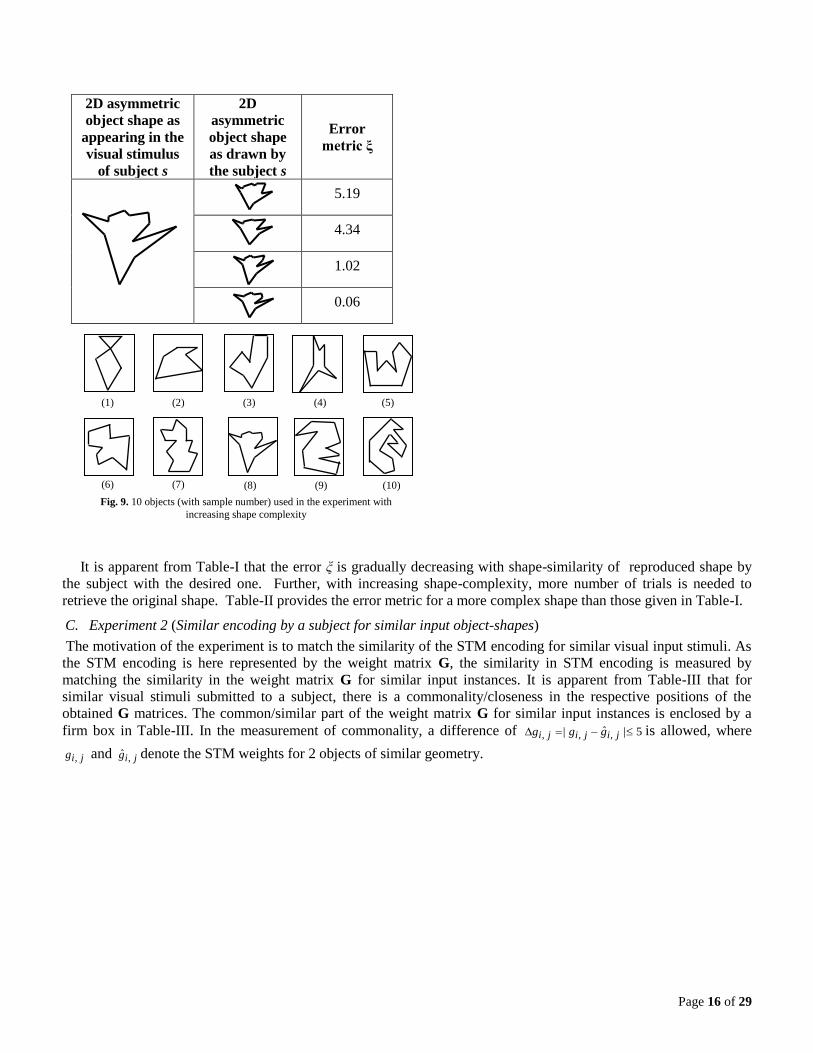
TABLE II. ERROR METRIC ξ FOR MORE COMPLEX SHAPE
Page 16 of 29
2D asymmetric
object shape as
appearing in the
visual stimulus
of subject s
2D
asymmetric
object shape
as drawn by
the subject s
Error
metric ξ
5.19
4.34
1.02
0.06
It is apparent from Table-I that the error ξ is gradually decreasing with shape-similarity of reproduced shape by
the subject with the desired one. Further, with increasing shape-complexity, more number of trials is needed to
retrieve the original shape. Table-II provides the error metric for a more complex shape than those given in Table-I.
C. Experiment 2 (Similar encoding by a subject for similar input object-shapes)
The motivation of the experiment is to match the similarity of the STM encoding for similar visual input stimuli. As
the STM encoding is here represented by the weight matrix G, the similarity in STM encoding is measured by
matching the similarity in the weight matrix G for similar input instances. It is apparent from Table-III that for
similar visual stimuli submitted to a subject, there is a commonality/closeness in the respective positions of the
obtained G matrices. The common/similar part of the weight matrix G for similar input instances is enclosed by a
firm box in Table-III. In the measurement of commonality, a difference of 5|ˆ| ,,, jijiji ggg is allowed, where
jig , and jig ,ˆ denote the STM weights for 2 objects of similar geometry.
(1) (2) (3) (4) (5)
(6) (7) (8) (9) (10)
Fig. 9. 10 objects (with sample number) used in the experiment with
increasing shape complexity
Page 17 of 29
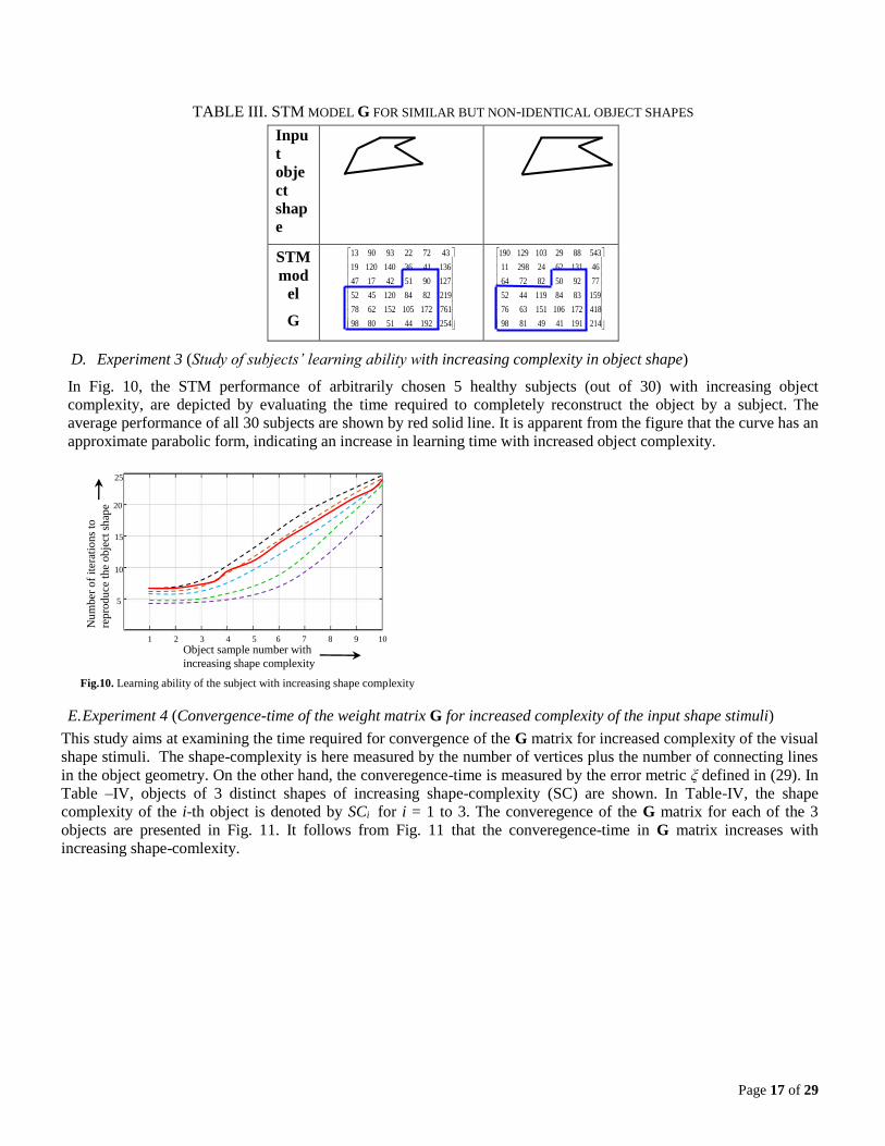
TABLE III. STM MODEL G FOR SIMILAR BUT NON-IDENTICAL OBJECT SHAPES
Inpu
t
obje
ct
shap
e
STM
mod
el
G
25419244518098
7611721051526278
21982841204552
1279051421747
136413614012019
437222939013
21419141498198
4181721061516376
15983841194452
779250827264
46131622429811
5438829103129190
D. Experiment 3 (Study of subjects’ learning ability with increasing complexity in object shape)
In Fig. 10, the STM performance of arbitrarily chosen 5 healthy subjects (out of 30) with increasing object
complexity, are depicted by evaluating the time required to completely reconstruct the object by a subject. The
average performance of all 30 subjects are shown by red solid line. It is apparent from the figure that the curve has an
approximate parabolic form, indicating an increase in learning time with increased object complexity.
E. Experiment 4 (Convergence-time of the weight matrix G for increased complexity of the input shape stimuli)
This study aims at examining the time required for convergence of the G matrix for increased complexity of the visual
shape stimuli. The shape-complexity is here measured by the number of vertices plus the number of connecting lines
in the object geometry. On the other hand, the converegence-time is measured by the error metric ξ defined in (29). In
Table –IV, objects of 3 distinct shapes of increasing shape-complexity (SC) are shown. In Table-IV, the shape
complexity of the i-th object is denoted by SCi for i = 1 to 3. The converegence of the G matrix for each of the 3
objects are presented in Fig. 11. It follows from Fig. 11 that the converegence-time in G matrix increases with
increasing shape-comlexity.
1 2 3 4 5 6 7 8 9 10
5
10
15
20
25
Object sample number with
increasing shape complexity
Nu
mber
of
iter
atio
ns
to
rep
rodu
ce t
he
ob
ject
sh
ape
Fig.10. Learning ability of the subject with increasing shape complexity

Page 18 of 29
TABLE IV. OBJECT SHAPES ACCORDING TO THE INCREASED SHAPE COMPLEXITY (SC1 < SC2< SC3 )
Shape
Comple
xity
SC1 SC2 SC3
2D
asymme
tric
object
shapes
F. Experiment 5 (Abnormality in G matrix for the subjects with brain impairment)
Here, the experiment is performed on 2 groups of subjects: people with i)temporal lobe epilepsy (Fig. 12(a)),
ii)Alzheimer’s disease/amnesia with impairment in pre-frontal regions (Fig. 12(b)). Here, the same input shape-
stimulus is submitted to the subject in 3 separate experiments performed on 3 different dates with a gap of 10 days
between 2 consecutive experiments, and the convergence in G matrix is determined in terms of the error metric .'E
A similarity measure in the G matrix after convergence for the above 3 experiments on the same subject is
ascertained. It is observed from Fig. 12(b) that the G matrices obtained after convergence have least similarity for
people with Alzheimer’s diesease with pre-frontal impairment. However, people with temporal lobe epilepsy have
similarity in the converged G matrices for 3 experiments (Fig. 12(b)), as happens to be for normal/healthy subjects.
The G matrices for two persons (one with prefrontal lobe Amnesia, and one with temporal lobe eplilepsy), obtained
after converegence of 3 experiments are illustrated in Fig. 12(a) and (b), where the regions (area) of converegence in
the G matrices for 3 experiments are indicated by hatched lines. It is apparent from Fig. 12(a) that the commonality
in the converged areas in G matrix for patients with Prefrontal lobe Amnesia is insignificantly small. The
dissimilarity in the G matrix (represented in blue) may be used as a measure of degree of STM impairment.
V. BIOLOGICAL IMPLICATIONS
To compute the intra-cortical distribution of the electric activity from the surface EEG data, a special software, called
eLORETA (exact Low Resolution brain Electromagnetic TomogrAphy) [63] is employed. The eLORETA is a linear
(a)
(b)
Experimental
Day1
Experimental
Day 2
Experimental
Day 3
Experimental
Day1
Experimental
Day 2
Experimental
Day 3
Fig. 12. Dissimilar Region of the G matrix in successive trials obtained for (a) a patient with pre-frontal lobe amnesia and (b) a patient with temporal
lobe epilepsy
Fig.11. Convergence of the error metric ξ (and weight matrix G) over time
with increased shape complexity
Erro
r M
etr
ic ξ
Number of trials 0 3 6 9 12 15 18 21

Page 19 of 29
inverse solution method capable of reconstructing cortical electrical activity with correct localization from the scalp
EEG data even in the presence of structured noise [64]. For the present experiment, the selected artifact-free EEG
segments are used to evaluate the eLORETA intracranial spectral density in the frequency range 0-30 Hz with a
resolution of 1 Hz. As indicated in Fig. 8, the entire experiment for a single trial is performed in 60 seconds (60,000
ms), comprising 10 seconds for memory encoding and 50 seconds for memory recall. The 60 seconds interval is
divided into 600 time-frames of equal length (100ms) by the e-LORETA software. In addition, the negativity of
N400 [73] is checked after each learning epoch to confirm that the brain response obtained is due to neurons
participating in STM learning.
The following biological implications directly follow from the eLORETA solutions and the negativity of the
N400 signal.
1. Fig. 13 provides the eLORETA solutions for the source localization problem during memory encoding and recall
phases. It is observed from the eLORETA scalp map (Fig. 13) that the electric neuronal activity is higher in the
occipital region for the first two time frames, demonstrating the iconic memory (IM) encoding of the visually
perceived object-shape for approximately 200 ms duration. For the next 90 time-frames (9000 milliseconds), the pre-
frontal cortex remains highly active, revealing the STM encoding during this interval of time. In the remaining time
frames, a significant increase in current density is observed in the pre-frontal and parietal cortex bilaterally, which
signifies the involvement of these two lobes in task-planning for the hand-drawing.
2. To check the N400 Repetition effect [74] during
STM learning, each subject is elicited with the same
object-shape repetitively until she learns to reproduce the
original shape presented to her, and the N400 pattern is
observed during each learning stage. It is observed that the
N400 response to the first trial exhibits the largest
negative peak with decreasing negativity in successive
trials. Fig. 14 represents the N400 dynamics over
repetitive trials for the same subject stimulated with the
same stimulus. Simultaneously, the eLORETA solutions,
represented by topographic maps in Fig. 14, indicate the
increasing neuronal activity in the pre-frontal cortex during the learning phase.
3. The N400 negativity with increased complexity in shape learning, also increases at a given learning epoch. The
increased negativity in N400 for the shapes listed in Table-IV are shown in Fig. 15.
Fig. 14. N400 repetition effects along with eLORETA solutions for successive trials: (a) trial 1 (b) trial 2 and (c) trial 3
A: Anterior
B: Middle
C: Posterior
A: Anterior
B: Middle
C: Posterior
Fig. 13. eLORETA tomography based on the current electric density (activity) at cortical voxels

Page 20 of 29
VI. PERFORMANCE ANALYSIS
This section provides an experimental basis for performance analysis and comparison of the proposed Type 2 Fuzzy
Set (T2FS) induced mapping techniques with the traditional/existing ones. Here too the performance of the proposed
and the state-of-the-art algorithms have been analyzed using MATLAB-16b toolbox, running under Windows-10 on
Intel Octacore processor with clock speed 2 GHz and 64 GB RAM.
TABLE V. COMPARISON OF'E OBTAINED BY THE PROPOSED MAPPING METHODS AGAINST STANDARD MAPPING
TECHNIQUES
Mapping
technique used in
the last 2 stages
of the Training
Network
'E
Run-time of the
Training
algorithm in a
IBM PC Dual-core
Machine
Proposed GT2FS 0.033 92.15milliseconds
Proposed IT2FS 0.062 34.23 milliseconds
Vertical slice
GT2FS [53] 0.081 94.62 milliseconds
Z slice GT2FS [51] 1.00 95.17 milliseconds
Z slice GT2FS [52] 1.001 95.51 milliseconds
SA-GT2FGG [65] 0.98 95.97 milliseconds
GT2FS [66] 1.40 96.87 milliseconds
IT2FS [66] 2.59 37.66 milliseconds
Type-1 Fuzzy Sets 7.62 36.34 milliseconds
LSTM [67] 4.59 120 milliseconds
CNN [68] 4.70 114 milliseconds
Polynomial
Regression
of order 10
4.95 101.40milliseconds
Polynomial
Regression
of order 20
4.70 101.30milliseconds
Polynomial
Regression
of order 25
4.00 120.20milliseconds
SVM with
polynomial Kernel 3.21 54.23 milliseconds
SVM with
Gaussian Kernel 3.001 53.87 milliseconds
BPNN 4.011 65.33 milliseconds
Fig. 15. Increasing N400 negativity with increasing shape complexity
Time in ms
Am
pli
tud
e in
µv
SC1 < SC2< SC3

Page 21 of 29
A. Performance Analysis of the proposed T2FS methods
To study the relative performance of the proposed Type-2 fuzzy mapping techniques with the existing methods, the
error metric 'E and runtime of the training algorithm are used for comparison. During comparison, the type-2 fuzzy
model present in the last 2 stages of the training and the test model only are replaced by existing deep learning or
other models. The rest of training and testing are similar to the present work. Table-V includes the results of 'E obtained by the 2 proposed T2FS based mapping techniques against traditional type-1 and type-2 fuzzy [51-
53],[65-66] algorithms, standard deep learning algorithms, including Long Short-Term Memory (LSTM) [67] and
Convolutional Neural Network (CNN) [68], and traditional non-fuzzy mapping algorithms including N-th order
Polynomial regression [75] of the form:1
Ni
ii
P q z
for real iq , Support Vector Machine (SVM) with polynomial
Kernel [69], SVM with Gaussian Kernel [70] and the Back Propagation Neural Network (BPNN) [71], realized and
tested for the present application. The experiment was performed on 35 subjects, each participating in 10 learning
sessions, comprising 10 stimuli, covering 35 ×10 ×10 = 3500 learning instances. It is observed from Table-V that the
proposed GT2FS based mapping technique outperforms its nearest competitors by an 'E of ~ 1.5%. In Table-V, we
also observe that the IT2FS based mapping technique takes the smallest run- time (~34 ms), when compared with the
other mapping methods. In addition, the proposed GT2FS-based method requires 92.15 ms, which is comparable to
the run-time of most of the T2FS techniques.
B. Computational Performance Analysis of the proposed T2FSmethods
Computational performance of T2FS induced mapping techniques is generally determined by the total number of t-
norm and s-norm computations [65]. In the computational complexity analysis, given in Table VI, the order of
complexity of each technique is listed, where n is the number of GT2FSs (i.e., number of features), M is the number
of discretization in the y axis and I is the number of z-slices (considered only in the existing z-slice based
approaches).
TABLE VI. ORDER OF COMPLEXITY OF THE PROPOSED T2FS ALGORITHMS AND OTHER COMPETITIVE MAPPING
TECHNIQUES
T2FS based Mapping
Algorithms
Order of
Complexity
Proposed IT2FS O(n)
Proposed GT2FS O(M.n)
Vertical slice GT2FS [53] O( nM )
Z slice GT2FS [51] O(M.n.I)
Z slice GT2FS [52] O(M.n.I)
C.Statistical Validation using Wilcoxon signed-rank test
A non-parametric Wilcoxon signed-rank test [72] is employed to statistically validate the proposed mapping
techniques using 'E as a metric on a single database, prepared at Artificial intelligence Laboratory of Jadavpur
University. Let, Ho be the null hypothesis, indicating identical performance of a given algorithm-B with respect to a
reference algorithm-A. Here, A = any one of the two proposed type-2 fuzzy mapping techniques and B = any one of
the 7 algorithms listed in Table VII. To statistically validate the null hypothesis Ho, we evaluate the test statistic W by
].)[sgn(1
,, i
rT
iiBiA rEEW
(30)
where iAE , and iBE , are the values of ,'E obtained by algorithms A and B respectively at i-th experimental instance. Tr
is the total number of experimental instances and ri denotes the rank of the pairs at i-th experimental instance, starting
with the smallest as 1.

Page 22 of 29
TABLE VII. RESULTS OF STATISTICAL VALIDATION WITH THE PROPOSED METHODS AS REFERENCE, ONE AT A TIME
Existing Methods
Reference method
Proposed
IT2FS
Proposed
GT2FS
Proposed IT2FS -
Proposed GT2FS -
Vertical slice
GT2FS [53] -
+
Z slice GT2FS
[51]
- +
Z slice GT2FS
[52]
- +
SA-GT2FGG [65] + +
GT2FS [66] + +
IT2FS [66] + +
Type-1 Fuzzy Sets + +
Table VII is aimed at reporting the results of the Wilcoxon signed-rank test, considering either of the proposed
IT2FS and GT2FS as the reference algorithm. The plus (minus) sign in Table VII represents that the W values (i.e.,
the difference in errors) of an individual method with the proposed method as reference is significant (not
significant). Here, 95% confidence level is achieved with the degree of freedom 1, studied at p-value greater than
0.05.
D. Optimal Parameter Selection and Robustness Study
For robustness study, the parameters used in the proposed training algorithm are optimized with respect to a
judiciously selected objective function. Since E represents the error metric at the last trial, one possible objective
measure could be
| | .J E (31)
where E indirectly involves the following parameter set: = ,{ , , }.1 Since J is not a direct function of the
above parameters, traditional derivative-based optimization is not feasible. Any meta-heuristic algorithm, however,
can serve the purpose well. Differential Evolution (DE) algorithm has been chosen here for its small code-length, low
run-time complexity, good computational accuracy, and above all the authors’ familiarity with it for several years
[79], [96].
DE maintains a fixed population-size of parameter vectors (trial solutions) over the iterations. The components of
the parameter vectors are initialized in a uniformly random manner over user-defined individual parametric space.
The parameter vectors of the DE-target-to-best algorithm employed are evolved through a process of mutation with
scale factor F = 0.8 and binomial crossover/recombination with crossover rate CR = 0.7 in two successive steps. The
resulting vectors obtained after recombination are referred to as Target vectors. For each parameter vector, one target
vector is obtained. Next, the fitness of the evolved target vector and the corresponding trial solution are measured and
the member with better fitness is redefined as the resulting parameter vector for the next step of evolution. The
evolution of trial solutions is continued until the algorithm converges with a predefined error-limit of 0.001, where
the error-limit represents the absolute difference of fitness measure of the best-fit solution of the last and the current
generations. Fig. 16 provides a schematic overview of optimal parameter selection using DE.
Page 23 of 29
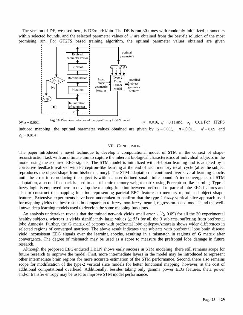
The version of DE, we used here, is DE/rand/1/bin. The DE is run 30 times with randomly initialized parameters
within selected bounds, and the selected parameter values of are obtained from the best-fit solution of the most
promising run. For GT2FS based training algorithm, the optimal parameter values obtained are given
by 0.002, ,016.0 0.11 and 1 0.01. For IT2FS
induced mapping, the optimal parameter values obtained are given by 0.003, ,011.0 0.09 and
014.01 .
VII. CONCLUSIONS
The paper introduced a novel technique to develop a computational model of STM in the context of shape-
reconstruction task with an ultimate aim to capture the inherent biological characteristics of individual subjects in the
model using the acquired EEG signals. The STM model is initialized with Hebbian learning and is adapted by a
corrective feedback realized with Perceptron-like learning at the end of each memory recall cycle (after the subject
reproduces the object-shape from his/her memory). The STM adaptation is continued over several learning epochs
until the error in reproducing the object is within a user-defined small finite bound. After convergence of STM
adaptation, a second feedback is used to adapt iconic memory weight matrix using Perceptron-like learning. Type-2
fuzzy logic is employed here to develop the mapping function between prefrontal to parietal lobe EEG features and
also to construct the mapping function representing parietal EEG features to memory-reproduced object shape-
features. Extensive experiments have been undertaken to confirm that the type-2 fuzzy vertical slice approach used
for mapping yields the best results in comparison to fuzzy, non-fuzzy, neural, regression-based models and the well-
known deep learning models used to develop the same mapping functions.
An analysis undertaken reveals that the trained network yields small error 'E (≤ 0.09) for all the 30 experimental
healthy subjects, whereas it yields significantly large values (≥ 53) for all the 3 subjects, suffering from prefrontal
lobe Amnesia. Further, the G matrix of persons with prefrontal lobe epilepsy/Amnesia shows wider differences in
selected regions of converged matrices. The above result indicates that subjects with prefrontal lobe brain disease
yield inconsistent EEG signals over the learning epochs, resulting in a mismatch in regions of G matrix after
convergence. The degree of mismatch may be used as a score to measure the prefrontal lobe damage in future
research.
Although the proposed EEG-induced DBLN shows early success in STM modeling, there still remains scope for
future research to improve the model. First, more intermediate layers in the model may be introduced to represent
other intermediate brain regions for more accurate estimation of the STM performance. Second, there also remains
scope for modification of the type-2 vertical slice models for better functional mapping, however, at the cost of
additional computational overhead. Additionally, besides taking only gamma power EEG features, theta power
and/or transfer entropy may be used to improve STM model performance.
Fig. 16. Parameter Selection of the type-2 fuzzy DBLN model
Recalled
object
geometric
features
Stop
Type-2
Fuzzy DBLN
Model
'E
Input object
geometric
features
Initialization of parameter
Mutation
Recombination E’< δ2
No
1 Selection
Evolved
parameter vector
optimal
parameters
DE

Page 24 of 29
Acknowledgment The authors gratefully acknowledge the funding they received from the UPE-II Project in Cognitive Science offered by University Grants Commission (UGC) to Jadavpur University.

Page 25 of 29
APPENDIX
This Appendix provides the simulation results of geometric feature extraction introduced in Section-II.
Gaussian filtering
Canny edge detection
Grayscale image of
the input object shape
Lengths: ,402,246,114,304,289 EFDECDBCAB
268,438,554 HAGHFG
Angles: ,13,307,34,215,29 EDCBA
.262,5.13,209 HGF
Computation of line length and
angle between adjacent sides
A (697,
53)
(455, 211)
B (151, 211)
C (246, 275) D E (14,
356)
F
(414,
320) (920, 546)
G
H (567, 287)
Line End Point co-ordinate
determination
Line parameter (ρ, α)
evaluation by Hough transform

Page 26 of 29
REFERENCES
[1] M. Mishkin, and T. Appenzeller, The anatomy of memory. Scientific American, Incorporated, 1987. [2] A. Baddeley, “Working memory and conscious awareness,” Theories of Memory, pp. 11-20, 1992. [3] A. Mollet, "Fundamentals of human neuropsychology." J. of Undergraduate Neuroscience Education, vol. 6, p:
2, 2008. [4] N. M. Van Strien, N. L. M. Cappaert, and M. P. Witter. "The anatomy of memory: an interactive overview of
the parahippocampal-hippocampal network." Nature reviews. Neuroscience 10, vol.4, p: 272, 2009. [5] J. Ward, The student's guide to cognitive neuroscience. Psychology Press, 2015. [6] W. R . Klemm, Atoms of Mind: The" ghost in the Machine" Materializes. Springer Science & Business Media,
2011. [7] W. R. Klemm, "The Quest." Atoms of Mind. Springer Netherlands, pp. 1-17, 2011. [8] K. Numata, Y. Nakajima, T. Shibata, and S. Shimizu, "EEG Gamma Band Is Asymmetrically Activated by
Location and Shape Memory Tasks in Humans." J. of the Japanese Physical Therapy Association, vol. 5, pp. 1-5, 2002.
[9] T. J. Lloyd-Jones, M. V. Roberts, E. C. Leek, N. C. Fouquet andE. G. Truchanowicz, “The time course of activation of object shape and shapeþcolour representations during memory retrieval.” PloS One, vol. 7, 2012.
[10] J. M. Fuster, R. H. Bauer, and J.P. Jervery, “Functional interactions between inferotemporal and prefrontal cortex in a cognitive task”. Brain research 330. Vol. 2, pp. 299-307, 1985.
[11] J. Quintana, J. M. Fuster, and Y. Javier "Effects of cooling parietal cortex on prefrontal units in delay tasks." Brain research 503. Vol. 1 pp. 100-110, 1989.
[12] S. Zeki, and S. Shipp, "The functional logic of cortical connections." Nature 335. pp. 311-317, 1988. [13] M. Mesulam, "A cortical network for directed attention and unilateral neglect." Annals of neurology 10. Vol. 4,
pp. 309-325, 1981. [14] W. B. Barr, "Examining the right temporal lobe's role in nonverbal memory." Brain and cognition 35. Vol. 1
pp.26-41, 1997. [15] M. Corbetta, F. M. Miezin, S. Dobmeyer, G. L. Shulman, and S. E. Petersen, "Selective and divided attention
during visual discriminations of shape, color, and speed: functional anatomy by positron emission tomography." J. of neuroscience. Vol. 8, pp. 2383-2402, 1991.
[16] S. C. Baker, C. D. Frith, S. J. Frackowiak, and R. J. Dolan, "Active representation of shape and spatial location in man." Cerebral Cortex. Vol. 4, pp. 612-619, 1996.
[17] K. H. Lee, L. M. Williams, M. Breakspear, and E.Gordon, "Synchronous gamma activity: a review and contribution to an integrative neuroscience model of schizophrenia." Brain Research Reviews. Vol. 1, pp. 57-78, 2003.
[18] J. R. Vidal, M. Chaumon, J. K. O'Regan, and C.Tallon-Baudry, "Visual grouping and the focusing of attention induce gamma-band oscillations at different frequencies in human magnetoencephalogram signals." J. of Cognitive Neuroscience. Vol. 11, pp. 1850-1862, 2006.
[19] D. Senkowski, and C. S. Herrmann. "Effects of task difficulty on evoked gamma activity and ERPs in a visual discrimination task." Clinical Neurophysiology . Vol. 11, pp. 1742-1753, 2002.
[20] M. K. Rieder, B. Rahm, J. D. Williams, and J. Kaiser, "Human gamma-band activity and behavior." International Journal of Psychophysiology 79.1 (2011): 39-48.
[21] P. J. Uhlhaas, and W. Singer, "Neural synchrony in brain disorders: relevance for cognitive dysfunctions and pathophysiology." Neuron 52.1 (2006): 155-168.
[22] W. Ross Ashby, Design for a brain: The origin of Adaptive Behaviour, John Wiley and Sons, 1954. [23] R. C. Atkinson, and R. M. Shiffrin, “Human memory: A proposed system and its control processes,” Psychology
of Learning and Motivation, vol. 2, pp. 89-195, 1968. [24] E. Tulving, and J. Psotka, “Retroactive inhibition in free recall: Inaccessibility of information available in the
memory store,” J. of Experimental Psychology, vol. 87, pp. 1-8, 1971. [25] M. A. Conway, Cognitive models of memory, MIT Press, 1997. [26] A. D. Baddeley, Essentials of human memory, Psychology Press, 1999. [27] A. Baddeley, "The episodic buffer: a new component of working memory?,” Trends in Cognitive Sciences, vol.
4, pp. 417-423, 2000. [28] B. J. Baars, and S. Franklin, “How conscious experience and working memory interact,” Trends in Cognitive
Sciences, vol. 7, pp. 166-172, 2003. [29] D. Vernon, Artificial Cognitive Systems, MIT Press, Cambridge, 2014. [30] C. Başar-Eroglu, D.Strüber, M. Schürmann, M. Stadler, & E.Başar, "Gamma-band responses in the brain: a short
review of psychophysiological correlates and functional significance." Int. J. of Psychophysiology. Vol. 1, pp. 101-112, 1996.
[31] C. T. Baudry, and O. Bertrand, "Oscillatory gamma activity in humans and its role in object representation." Trends in cognitive sciences, vol. 4, pp. 151-162 1999.
[32] W. Klimesch, "EEG alpha and theta oscillations reflect cognitive and memory performance: a review and analysis." Brain research reviews, vol. 2, pp. 169-195, 1999.

Page 27 of 29
[33] C. S. Herrmann, M. H. J. Munk, and A. K. Engel, "Cognitive functions of gamma-band activity: memory match and utilization." Trends in cognitive sciences, vol. 8,pp. 347-355, 2004.
[34] P. Sauseng, W. Klimesch, M. Schabus and M.Doppelmayr, "Fronto-parietal EEG coherence in theta and upper alpha reflect central executive functions of working memory." Int. J. of Psychophysiology. Vol. 2 pp. 97-103, 2005.
[35] W. Klimesch, P. Sauseng, and S. Hanslmayr, "EEG alpha oscillations: the inhibition–timing hypothesis." Brain research reviews. Vol. 1, pp. 63-88, 2007.
[36] N. Kopell, M. A. Whittington, and M. A. Kramer. "Neuronal assembly dynamics in the beta1 frequency range permits short-term memory." In theProc. of the National Academy of Sciences, pp. 3779-3784, 2011.
[37] R. Van den Berg, H. Shin, W. C. Chou, R. George, and W. J.Ma, “Variability in encoding precision accounts for visual short-term memory limitations." In the Proc. of the National Academy of Sciences, pp. 8780-8785, 2012.
[38] W. Nan, J. P. Rodrigues, J. Ma, X. Qu, F. Wan, P. I. Mak, and A. Rosa, "Individual alpha neurofeedback training effect on short term memory." Int. J. of psychophysiology. Vol. 1, pp. 83-87, 2012.
[39] J. J. LaRocque, J. A. Lewis-Peacock, A. T. Drysdale, K. Oberauer, and B. R.Postle, "Decoding attended information in short-term memory: an EEG study." J. of Cognitive Neuroscience. vol. 1 , pp. 127-142, 2013.
[40] R. N. Roy, S. Bonnet, S. Charbonnier and A.Campagne, "Mental fatigue and working memory load estimation: interaction and implications for EEG-based passive BCI." In the Proc. of Int. Conf. on Engineering in Medicine and Biology Society (EMBC), IEEE, 2013.
[41] G. Luksys, M. Fastenrath, D. Coynel, V. Freytag, L. Gschwind, A. Heck, and M. Scherer, "Computational dissection of human episodic memory reveals mental process-specific genetic profiles." In theProc. of the National Academy of Sciences35, pp. E4939-E4948, 2015.
[42] M. Ono, H. Furusho, and K. Iramina. "Analysis of the complexity of EEG during the short-term memory task." In the Proc. of Biomedical Engineering Int. Conference (BMEiCON), 2015 8th, IEEE, 2015.
[43] Y. Singh, J. Singh, R. Sharma, and A.Talwar, "FFT transformed quantitative EEG analysis of short term memory load." Annals of neurosciences. Vol. 3, p : 176, 2015.
[44] S. Slotnick, "Frontal-occipital interactions during visual memory." file:///G:/phd%20work/SSCI/iconic%20memory%20at%20occipital%20lobe/Frontaloccipital%20interactions%20during%20visual%20memory.html.
[45] W. Gerstner, “Hebbian Learning and Plasticity”, From neuron to Cognition via Computational Neuroscience, MIT Press, Cambridge, Chapter 9, 2011.
[46] A. Konar, Computational intelligence: principles, techniques and applications. Springer, 2006. [47] R. C. O'Reilly and K. A. Norman. "Hippocampal and neocortical contributions to memory: Advances in the
complementary learning systems framework." Trends in cognitive sciences, vol. 6, pp. 505-510, 2002. [48] S. E. Hyman, R. C. Malenka, and E. J. Nestler. "Neural mechanisms of addiction: the role of reward-related
learning and memory." Annu. Rev. Neurosci., vol. 29, pp. 565-598, 2006. [49] G. J. Klir and B. Yuan, Fuzzy Sets and Fuzzy Logic: Theory and Applications, Pretice-Hall, 1997. [50] J. Mendel, and D. Wu, Perceptual computing: Aiding people in making subjective judgments. vol. 13, John
Wiley & Sons, 2010. [51] J. M. Mendel, "General type-2 fuzzy logic systems made simple: a tutorial." IEEE Trans. Fuzzy Systems 22, vol.
5, pp. 1162-1182, 2014. [52] C. Wagner, and H. Hagras, "Toward general type-2 fuzzy logic systems based on zSlices." IEEE Trans. Fuzzy
Systems 18, vol. 4 pp: 637-660, 2010. [53] J. M. Mendel and R. I B. John, "Type-2 fuzzy sets made simple." IEEE Trans. Fuzzy Systems 10, vol. 2, pp: 117-
127, 2002. [54] I. Goodfellow, Y. Bengio, A. Courville, and Y. Bengio. Deep learning. Vol. 1. Cambridge: MIT press, 2016. [55] J. B. Scarborough, Numerical Mathematical. Oxford and IBH Publishing, 1955. [56] S. Haykin, Neural networks: a comprehensive foundation. Prentice Hall PTR, 1994. [57] C. Werner, U. Wegmuller, T. Strozzi, and A. Wiesmann. "Interferometric point target analysis for deformation
mapping." In the proc. of Geoscience and Remote Sensing Symposium, vol. 7, pp. 4362-4364. IEEE, 2003. [58] S. L. Kappel, D. Looney, D. P. Mandic, and P. Kidmose. "Physiological artifacts in scalp EEG and ear-
EEG." Biomedical Engg. online 16, p:103, 2017. [59] D. Wu, “A Constraint Representation Theorem for Interval Type-2 Fuzzy Sets Using Convex and Normal
Embedded Type-1 Fuzzy Sets, and Its Application to Centroid Computation”, in: Proceedings of World Conference on Soft Computing, San Francisco, CA, May 2011.
[60] R. C. Malenka, ed., Intercellular Communication in the Nervous System, Academic Press, 2009. [61] L. Ghosh, A. Konar, P. Rakshit, S. Parui, A. L. Ralescu, A. K. Nagar, “P-300 and N-400 induced decoding of
learning skill of driving learners using Type-2 Fuzzy Sets”, in the Proc. of Int. IEEE conf. on Fuzzy Systems (Fuzz-IEEE), pp. 1-8, 2018.
[62] G. H. Klem, H. O. Luders, H. H. Jasper and C. Elger, “The ten-twenty electrode system of the International Federation”, Electroencephalogr Clin Neurophysiol, vol. 52, pp. 3-6, 1999.
[63] R. D. Pascual-Marqui, D. Lehmann, M. Koukkou, K. Kochi, P. Anderer, et al.“Assessing interactions in the brain with exact low resolution electromagnetic tomography”. Phil Trans R Soc A 369: 3768–3784, 2011.
Page 28 of 29
[64] R. D. Pascual-Marqui, “Discrete, 3D distributed, linear imaging methods of electric neuronal activity. Part 1: exact, zero error localization”, arXiv:0710.3341[math-ph]. Arxiv website. Available: http://arxiv.org/pdf/0710.3341, 2007.
[65] J. Andreu-Perez, F. Cao, H. Hagras and G. Z. Yang, “A Self-Adaptive Online Brain Machine Interface of a Humanoid Robot through a General Type-2 Fuzzy Inference System,” IEEE Trans. on Fuzzy Systems, vol. 9, 2016.
[66] A. Saha, A. Konar, and A. K. Nagar. "EEG Analysis for Cognitive Failure Detection in Driving Using Type-2 Fuzzy Classifiers." IEEE Trans. on Emerging Topics in Comp. Int., pp: 437-453, 2017.
[67] S. Hochreiter and J. Schmidhuber. "Long short-term memory." Neural computation, vol. 8, pp. 1735-1780, 1997. [68] K.Simonyan and A. Zisserman. "Very deep convolutional networks for large-scale image recognition." arXiv
preprint arXiv, pp. 1409-1556, 2014. [69] Y. W. Chang, C. J. Hsieh, K. W. Chang, M. Ringgaard and C. J. Lin. "Training and testing low-degree
polynomial data mappings via linear SVM." Journal of Machine Learning Research, vol. 11, pp. 1471-1490, 2010.
[70] B. Scholkopf, K. Sung, C. JC Burges, F. Girosi, P. Niyogi, T. Poggio, and V. Vapnik. "Comparing support vector machines with Gaussian kernels to radial basis function classifiers." IEEE trans. on Signal Processing, vol. 11, pp: 2758-2765, 1997.
[71] Z.Waszczyszyn and L. Ziemiański. "Neural networks in mechanics of structures and materials–new results and prospects of applications." Computers & Structures, vol. 79, pp: 2261-2276, 2001.
[72] F. Wilcoxon, S. K. Katti, and R. A. Wilcox. "Critical values and probability levels for the Wilcoxon rank sum test and the Wilcoxon signed rank test." Selected tables in mathematical statistics, vol.1, pp.171-259, 1970.
[73] M. Kutas and K. D. Federmeier, “N400”, Scholerpedia, 4(10)2009,7790. [74] M. D. Rugg, “Event-related brain potentials dissociate repetition effects of high- and low-frequency words”.
Memory and Cognition, 18(4), 367-379, 1990. [75] C. L. Goodale, J. D. Aber and S. V. Ollinger. "Mapping monthly precipitation, temperature, and solar radiation
for Ireland with polynomial regression and a digital elevation model." Climate Research, vol. 1, pp: 35-49, 1998. [76] J. M. Mendel, M. R. Rajati and P. Sussner, “On clarifying some definitions and notations used for type-2 fuzzy
sets as well as some recommended changes”, Information Sciences, pp. 337-345 , 2016. [77] A. Khasnobish, A. Konar, D. N. Tibarewala, and A. K. Nagar. "Bypassing the natural visual-motor pathway to
execute complex movement related tasks using interval type-2 fuzzy sets." IEEE Trans. on Neural Sys. and Rehabilitation Engg., vol. 1,pp.91-105, 2017.
[78] D. Bhattacharya, A. Konar, and P. Das. "Secondary factor induced stock index time-series prediction using self-adaptive interval type-2 fuzzy sets." Neurocomputing, vol. 171, pp. 551-568, 2016.
[79] P. Rakshit, A. Konar, P. Bhowmik, I. Goswami, S. Das, L. C. Jain and A. K. Nagar, "Realization of an adaptive memetic algorithm using differential evolution and q-learning: a case study in multirobot path planning." IEEE Trans. Systems, Man, and Cybernetics: Systems 43, vol. no. 4, pp: 814-831, 2013.
[80] K. A. Ludwig, R. M. Miriani, N. B. Langhals, M. D. Joseph, D. J. Anderson, and D. R. Kipke. "Using a common average reference to improve cortical neuron recordings from microelectrode arrays." J. of neurophysiology, vol. 3, p: 1679, 2009.
[81] L. R. Squire, D. Berg, F.E. Bloom, S. D. Lac, A. Ghosh, N. C. Spitzer, Fundamental Neuroscience, Academic Press, Fourth Edition, 2013.
[82] Y. Jiang, D. Wu, Z. Deng, P. Qian, J. Wang, G. Wang, F.L. Chung, K.S. Choi, and S. Wang, "Seizure Classification from EEG Signals using Transfer Learning, Semi-Supervised Learning and TSK Fuzzy System." IEEE Trans. on Neural Sys. & Rehab. Engg., vol.12, pp.2270 – 2284, 2017.
[83] Y. Jiang, Z. Deng, F.L. Chung, G. Wang, P. Qian, K.S. Choi, and S. Wang, "Recognition of Epileptic EEG Signals Using a Novel Multiview TSK Fuzzy System," IEEE Trans. on Fuzzy Sys., vol. 25, pp.3-20, 2017.
[84] D. Wu, "Online and Offline Domain Adaptation for Reducing BCI Calibration Effort," IEEE Trans. on Human-Machine Sys., vol. 47, pp. 550-563, 2017.
[85] B. Green, "Canny edge detection tutorial." Retrieved: March6 (2002): 2005. [86] L. Xu, and E. Oja. "Randomized Hough transform (RHT): basic mechanisms, algorithms, and computational
complexities." CVGIP: Image understanding 57, no. 2, pp.131-154, 1993. [87] Y. Chen, Z. Lin, X. Zhao, G. Wang, and Y. Gu. "Deep learning-based classification of hyperspectral data." IEEE
J. of Selected topics in applied earth observations and remote sensing 7, vol. 6, pp: 2094-2107, 2014. [88] X. An, D. Kuang, X. Guo, Y. Zhao, and L. He. "A deep learning method for classification of EEG data based on
motor imagery." In Int. Conf. on Intelligent Computing, pp. 203-210. Springer, Cham, 2014. [89] S. Jirayucharoensak, S. Pan-Ngum, and P. Israsena. "EEG-based emotion recognition using deep learning
network with principal component based covariate shift adaptation." The Scientific World J., vol. 1, pp. 1-10, 2014.
[90] P. Bashivan, I. Rish, M. Yeasin, and N. Codella. "Learning representations from EEG with deep recurrent-convolutional neural networks." In the Proc. of Int. Conf. on Learning Representations, pp. 1- 15, 2015.
[91] P. Mehta, and D. J. Schwab. "An exact mapping between the variational renormalization group and deep learning." In the Proc. of Int. Conf. on Learning Representations, pp. 1- 8, 2014.

Page 29 of 29
[92] S. Fan, “Do Our Brains Use Deep Learning to Make sense of the World?”, https://singularityhub.com/2017/12/20/life-imitates-art-is-the-human-brain-also-running-deep-learning/#sm.0000f74204d3wdqrw591mrmxr5tqq.
[93] V. Mnih, K. Kavukcuoglu, D. Silver, A. A. Rusu, J. Veness, M. G. Bellemare, A. Graves et al. "Human-level control through deep reinforcement learning." Nature, vol. 518, pp: 529-533, 2015.
[94] Y. Sengupta, “Deep Learning and the Human Brain: Inspiration, Not Imitation”, https://dzone.com/articles/deep-learning-and-the-human-brain-inspiration-not, May, 2019.
[95] F. Chollet, Deep Learning mit Python und Keras: Das Praxis-Handbuch vom Entwickler der Keras-Bibliothek. MITP-Verlags GmbH & Co. KG, 2018.
[96] S. Das, A. Abraham, and A. Konar. "Automatic clustering using an improved differential evolution algorithm" IEEE Trans. on sys., man, and cybernetics-Part A: Systems and Humans, vol. 1, pp.:218-237, 2008.
Lidia Ghosh received her B.Tech. degree in Electronics and Tele-Communication Engineering from Bengal Institute of Technology, Techno India College in 2011, and her M. Tech. degree in Intelligent Automation and Robotics (IAR) from the department of Electronics and Tele-Communication Engineering, Jadavpur University, Kolkata in 2015. She was awarded Gold Medals for securing the highest percentage of marks in M. Tech in IAR in 2015. She is currently pursuing her Ph.D. in Cognitive Intelligence in Jadavpur University under the guidance of Prof. Amit Konar and Dr. Pratyusha Rakshit. Her current research interest includes deep learning, type-2 fuzzy sets, human memory formation, short and long term memory interactions, and biological basis of perception and scientific creativity.
Amit Konar (SM’ 2010) is currently a Professor in the department of Electronics and Tele-Communication Engineering, Jadavpur University, Kolkata, India. He earned his B.E. degree from Bengal Engineering College, Sibpur in 1983, and his M.E., M. Phil. and Ph.D. degrees, all from Jadavpur University in 1985, 1988 and 2004 respectively. Dr. Konar has published 15 books and over 350 research papers in leading international journals and conference proceeding. He has supervised 28 PhD theses and 262 Masters’ theses. He is a recipient of AICTE-accredited Career Award for Young Teachers for the period: 1997-2000. He is nominated as a Fellow of West Bengal Academy of Science and Engineering in 2010 and (Indian) National Academy of Engineering in 2015. Dr. Konar has been serving as an Associate Editor of several international journals, including
IEEE Transactions of Fuzzy Systems and IEEE Transactions of Emerging Trends in Computational Intelligence. His current research interest includes Cognitive Neuroscience, Brain-Computer Interfaces, Type-2 Fuzzy Sets and Multi-agent Systems.
Pratyusha Rakshit received the B. Tech. degree in Electronics and Communication Engineering (ECE) from Institute of Engineering and Management, India, and M.E. degree in Control Engineering from Electronics and Telecommunication Engineering (ETCE) Department, Jadavpur University, India in 2010 and 2012 respectively. She was awarded her Ph.D. (Engineering) degree from Jadavpur University, India in 2016. From August 2015 to November 2015, she was an Assistant Professor in ETCE Department, Indian Institute of Engineering Science and Technology, India. She is currently an Assistant Professor in ETCE Department, Jadavpur University. She was awarded Gold Medals for securing the highest percentage of marks in B. Tech. in ECE and among all the courses of M.E. respectively in 2010 and 2012. She was the recipient of CSIR Senior
Research Fellowship, INSPIRE Fellowship and UGC UPE-II Junior Research Fellowship. Her principal research interests include artificial and computational intelligence, evolutionary computation, robotics, bioinformatics, pattern recognition, fuzzy logic, cognitive science and human-computer interaction. She is an author of over 50 papers published in top international journals and conference proceedings. She serves as a reviewer in IEEE-TFS, IEEE-SMC: Systems, Neurocomputing, Information Sciences, and Applied Soft Computing.
Atulya K. Nagar received the D.Phil. degree in applied nonlinear mathematics from the University of York, York, U.K., in 1996. He is a Professor of mathematical sciences at Liverpool Hope University, Liverpool, U.K., where he is the Dean of the Faculty of Science. He received a prestigious Commonwealth Fellowship for the D.Phil. degree. His research interests include nonlinear mathematics, natural computing, and systems engineering. He is the Editor-in-Chief of International Journal of Artificial Intelligence and Soft Computing and serves on the editorial boards for a number of prestigious journals, including the Journal of Universal Computer Science. He was the Conference General Chair and member of the International Program Committee for several international conferences and was invited to deliver keynote lectures at a number of such
forums.