Mind the Gap: Disentangling Credit and Liquidity in Risk Spreads

Krista Schwarz* The Wharton School

University of Pennsylvania

October 27, 2017

Abstract

Wide and volatile interest rate spreads in the 2007-2009 financial crisis could represent concerns over asset liquidity or issuer solvency. To precisely identify the contribution of these two effects on interest rates, I propose a model-free measure of market liquidity, and use it to decompose euro-area sovereign bond and interbank spreads. Relating the measure to rates across countries reveals that German bonds benefit disproportionately from deteriorating liquidity. Additionally, cross-country bond return variation gives evidence of large and significant liquidity risk premia, the possibility that liquidity could be negatively correlated with marginal utility, something not captured by instantaneous liquidity measures.

JEL Classification: E44, G01, G12, G15 Keywords: market liquidity, interbank credit, liquidity risk, money markets, interest rates, financial crisis.

* Department of Finance, The Wharton School, University of Pennsylvania, 3620 Locust Walk, Philadelphia, PA 19104. Tel. 215-898-6087. E-mail: kschwarz@wharton.upenn.edu. I am grateful to an anonymous referee, Heitor Almeida, Andrew Ang, Charles Calomiris, Larry Glosten, Charles Jones, Ahn Le, Francis Longstaff and Suresh Sundaresan for their extremely helpful comments on this work, to the Department of Economics and Finance at Columbia Business School for funding the MTS data used in this paper, and to e-MID for generously sharing their data with me. I thank conference participants at the NBER Asset Pricing Meeting, Duke/UNC Asset Pricing, MTS, FIRS, and FRIAS. I also thank Sally Chen, Nicholas Hyde, Paola Ripamonti, and Ernie Vogt for valuable discussions about institutional detail and market functioning. All errors and omissions are my own.

1

Mind the Gap: Disentangling Credit and Liquidity in Risk Spreads

October 27, 2017

Abstract

Wide and volatile interest rate spreads in the 2007-2009 financial crisis could represent concerns over asset liquidity or issuer solvency. To precisely identify the contribution of these two effects on interest rates, I propose a model-free measure of market liquidity, and use it to decompose euro-area sovereign bond and interbank spreads. Relating the measure to rates across countries reveals that German bonds benefit disproportionately from deteriorating liquidity. Additionally, cross-country bond return variation gives evidence of large and significant liquidity risk premia, the possibility that liquidity could be negatively correlated with marginal utility, something not captured by instantaneous liquidity measures.

JEL Classification: E44, G01, G12, G15 Keywords: market liquidity, interbank credit, liquidity risk, money markets, interest rates, financial crisis.

2

The 2007-2009 financial crisis was marked by extraordinary interest rate spread widening

and heightened volatility in asset prices. One example is the increase in euro-area government

bond yields, which spiked to levels not seen since the introduction of the common currency in

1999. In the money market, spreads between unsecured interbank borrowing rates (EURIBOR)

and overnight-indexed swap (OIS) rates of comparable maturities reached their widest levels since

the inception of the OIS market, dramatically tightening financial conditions. Despite the

magnitude of these unusual interest rate movements, there has been a lack of consensus on the

dominant driver. One hurdle to identification is the difficulty in precisely capturing the risk

components in prices. This paper proposes a model-free measure of market liquidity formed

directly from asset prices, and uses it to parse these historic movements in interest rate spreads,

identifying a large role for liquidity.

Beyond the expected path of future short-horizon interest rates, it is difficult to empricially

determine what drives sovereign bond yields or interbank rates, especially at times of market

stress. Two possible influences that are explored in this paper are credit, reflecting compensation

for heightened default risk (Afonso, Kovner and Schoar (2011), Filipović and Trolle (2013),

Taylor and Williams (2009), Beber, Brandt and Kavajecz (2009), and McAndrews, Sarkar and

Wang (2008)), and market liquidity, reflecting trading conditions in asset markets (Michaud and

Upper (2008), Acharya and Skeie (2011)). The models of Heider and Hoerova (2009) and Heider,

Hoerova and Holthausen (2015) also discuss the role of these two risk components in interest rates.

Identifying the default and liquidity components in interest rates is important for portfolio

allocation and policy decisions. Investors with the longest investment horizons should prefer to

hold higher yielding assets if the elevated yields represent compensation for deteriorating market

conditions, but not necessarily if they represent a greater risk of loss due to default. From the

3

perspective of policymakers, efforts to improve market functioning could help to dampen the

effects of poor asset market liquidity on yields. For example, an exchange of more-liquid for less-

liquid bonds (such as in the Federal Reserve’s securities lending facility) could reduce liquidity

premia. On the other hand, if higher yields are attributable to a credit shock, then this argues for

addressing solvency.

This paper makes three contributions in the decomposition of interest rates into liquidity

and credit components. The first is a new market liquidity measure that captures liquidity broadly

by recovering all of the information embedded in yields that is not related to default risk. A

growing literature argues that model-driven liquidity indicators (e.g. bid-ask spreads) and liquidity

characteristics of assets (e.g. trading volume) do not capture all liquidity channels. For instance, a

bond could have low transactions costs and/or high volume today, but still have high liquidity risk.

Jankowitsch, Mösenbacher and Pichler (2006) find that conventional liquidity measures do not

adequately capture liquidity risk in the euro-area sovereign bond market. See also Friewald,

Jankowitsch and Subrahmanyam (2012) and Dick-Nielsen, Feldhütter and Lando (2012) in the

corporate bond market.

The proposed liquidity measure is model-free – it does not rely on single interpretation of

liquidity frictions. The measure is constructed directly from asset prices, and is defined as the

difference in yields between two duration-matched bonds that share an identical credit guarantee

from the German federal government, but differ in market liquidity. Specifically, the measure

compares the German federal government bond yield to that of its less-liquid agency counterpart,

KfW (Kreditanstalt für Wiederaufbau). This liquidity yield differential is referred to as the K-

spread. The K-spread therefore identifies any deviation in an asset’s price from its hold-to-maturity

value, fully capturing liquidity and liquidity risk effects impounded in prices. It is also tradable in

4

that an investor can form a portfolio comprised of a long KfW bond position and a corresponding

short German federal bond position. This position earns the “liquidity spread” and hedges against

credit fluctuations.

The second contribution is to use the K-spread as a common liquidity factor to parse the

components of rates for the euro-area sovereign bond and interbank markets. Researchers have

proposed theoretical models in which liquidity can have an important effect on bond yields,

especially during a crisis; Acharya and Skeie (2011), Favero, Pagano and von Thadden (2010) and

Manganelli and Wolswijk (2009). In the decomposition of sovereign bond yields, the K-spread is

used to identify liquidity effects in the cross section of euro-area countries, and so identification

relies on commonality in market liquidity. Chordia, Sarkar and Subrahmanyam (2005) and

Brunnermeier and Pedersen (2009) show that common factors drive liquidity premia across

various markets. Indeed, the K-spread explains more variation across different euro-area country

yields than several country-specific liquidity measures capture jointly. I find there is large variation

in the relative role of credit and liquidity by country, and that the liquidity effect varies in sign. In

particular, German bonds benefit disproportionately from a negative shock to euro-area liquidity.

I use the K-spread to decompose euro-area unsecured interbank rates in order to assess a

possible link between aggregate bond liquidity and money markets.1 Brunnermeier and Pedersen

(2009) and Bolton, Santos and Scheinkman (2011), model the relationship between aggregate

market liquidity and idiosyncratic funding liquidity to explain market features seen in the early

stages of the 2007-2009 financial crisis. To estimate this liquidity channel, I first obtain a novel

dataset of interbank transactions, with which I form a new bank-tiering credit measure and several

microstructure liquidity measures. The K-spread’s large role in interbank rates after controlling

1 Unsecured interbank rates, considered in this paper, are a close substitute to secured interbank rates (repo funding), which are directly affected by the liquidity premia of assets used as collateral.

5

for all interbank credit and liquidity measures gives strong empirical evidence for the general

equilibrium relationship between bond and funding markets.

The final contribution of this paper is to explicitly test the pricing of liquidity risk, in order

to better understand the nature of the large role for liquidity identified in interest rates over the

crisis. Liquidity risk is a forward-looking component of market liquidity that is not captured by

traditional measures. The concept of liquidity risk is proposed in the theoretical models of Acharya

and Pedersen (2005), Pastor and Stambaugh (2003) and Vayanos (2004), representing the

possibility that liquidity will dry up in the future at exactly the time when investors’ marginal

utility is at its highest. However, empirically, there are differing views on the importance of this

liquidity risk relative to the level of liquidity per se. In corporate bond markets, Lin, Wang and

Wu (2011) find that liquidity risk premia can help to explain corporate bond returns, whereas

Bongaerts, de Jong, and Driessen (2013) find that liquidity risk is priced in equity markets but not

in corporate bond markets.

Empirically, liquidity risk is defined as the covariance of government bond returns with

changes in market liquidity. The rich cross section and time series of euro-area sovereign bond

data makes it ideally suited to this estimation. Applying a two-step Fama MacBeth procedure, I

find a systematic relationship between liquidity factor sensitivity in bonds and their expected

returns across countries and maturities. Large and significant euro-area liquidity risk premia help

to explain the sizeable overall liquidity effect in interest rates in the 2007-2009 financial crisis.

The plan for the remainder of this paper is as follows. Section 1 introduces the framework

that underlies the empirical analysis. Section 2 introduces the data. Section 3 constructs the K-

spread liquidity measure and parses the relative euro-area sovereign bond yields into liquidity and

credit components. Section 4 identifies liquidity and credit effects in interbank interest rates.

6

Section 5 tests the pricing of liquidity risk premia in the euro-area sovereign bond market. Section

6 concludes with the paper’s contributions and implications.

1. A Simple Framework

This section introduces the particular euro-area interest rates considered, and describes a

simple structural model that isolates the risk component in these rates.

1.1 The Common Component in Euro-Area Interest Rates

Upon the introduction of the single euro currency in 1999, the European Central Bank

(ECB) became independently responsible for managing the common path of short-term interest

rates that are now shared by all euro-area member countries. The expected future path of euro-area

monetary policy anchors the hypothetical riskfree term structure of euro-denominated rates, in the

absence of liquidity effects, but this hypothetical yield curve is not directly observable. The focus

of this paper is to explain the variation in rates that is unrelated to the riskfree term structure.

During normal times, limited variation in the risk components of rates can make identification

challenging. However, substantial crisis-driven movement in market liquidity (the ease with which

a security is traded) and credit (the possibility that a financial instrument pays off below its face

value) presents a unique opportunity to cleanly identify their separate effects in interest rates.

There are two classes of interest rates that I aim to parse: (1) euro-area sovereign bond

yields, and (2) euro interbank borrowing rates (EURIBOR). Both classes of rates share a common

euro-area term structure. EURIBOR is the reference rate for large euro-area banks borrowing some

notional amount of euro currency from one another, uncollateralized, for a specified term.2 Euro-

2 EURIBOR is a survey rate of unsecured interbank euro borrowing rates compiled by the European Money Markets Institution (formerly the European Banking Federation) for eight maturities, from overnight- to one-year. LIBOR, also

7

area sovereign debt has a well-defined cross section of individual country bond yields, without a

single reference rate.

1.2 Isolating the Risk Component in Sovereign Bond Yields

First, to isolate the risk component in the sovereign bond market, consider a model in which

sovereign yields are expressed as a function of three components: the riskfree rate, expected

default and market liquidity.3 Specific measures of liquidity and credit will be proposed in Sections

2 and 3. The model relates individual country yields at each maturity to credit and liquidity as:

1 2cmt mt cm mt m cmt cmty r d (1)

where cmty is the sovereign bond yield for country c at maturity point m and time t, mtr is the

riskfree rate at maturity m, mt represents a single market liquidity factor and cmtd is the sovereign

default risk premium for country c. There is a single market liquidity factor and a common riskfree

rate across countries, and so these variables vary over time and by maturity but not by country,

reflected in the absence of a c subscript. The model’s representation is consistent with the euro-

area’s framework as a single currency union with an institutionally integrated secondary market.

Monetary union has prompted much market harmonization, such as the concentration of euro-

denominated sovereign debt transactions on a few dedicated platforms. Allowing the bonds of

different countries to load on a common liquidity factor leaves scope for divergent responses to an

aggregate liquidity shock. For instance, a flight-to-liquidity may support sovereign bonds that

already enjoy a relatively high level of liquidity as market participants concurrently shun less-

a survey of interbank borrowing, has been widely cited as manipulated to some degree by the contributing banks. To the extent that manipulation may have occurred in the EURIBOR survey, it is unlikely that the effect would be systematically related to the measures used in this paper, none of which settle to EURIBOR. If there were a systematic relationship, it is not clear in which direction this might shift the relative breakdown of liquidity versus credit. 3 Market liquidity is broadly defined as any influence on asset prices outside of credit.

8

liquid markets, thus increasing the liquidity discount in the less-liquid bond yields. In contrast,

default risk is idiosyncratic according to each country’s fiscal position, distinctly increasing for a

country as its federal budget deteriorates. For robustness, the decomposition in Section 3 also

includes an augmented model that allows for country-specific liquidity.

To measure each country’s relative sovereign yield premium within the model, without

taking a stance on the level of the unobserved riskfree rate, we can consider a yield spread for each

country-maturity pair. The yield spread is the difference between each country’s sovereign yield

and the euro-area weighted average yield.4 The weights are defined as 11

1

,cmcm

c mc

Qw

Q

where cm

Q is

the quantity of debt outstanding for each country c, at each maturity point m and c is a counter

variable indexing each of the countries for the purpose of computing the euro-area weighted

average.5 From Equation (1) we can deduce that:

' ' 1 ' 1 ' 2 ' ' ' '11 11 11 11

' 1 ' 1 ' 1 ' 1( ( ))cmt c m c mt cm c m c m mt m cmt c m c mt cmt c m c mtc c c cy w y w d w d w , (2)

which can be written more concisely as:

1 2cmt cm mt m cmt cmty d (3)

where cmty is the sovereign yield spread for country c, at the m-year maturity point, on day t.6

4 Correlations of euro-area bond yield levels rose around the time of monetary union and were high from then until the European debt crisis -- see Ehrmann, Fratzscher, Gürkaynak and Swanson (2011) -- largely reflecting the common component influenced by the state of euro-area monetary policy. 5 The maturity buckets comprise the total amount of debt outstanding for securities in the following duration ranges: 1-year bucket = 0.5 to 1.5, 2-year bucket = 1.5 to 2.5, 3-year = 2.5 to 3.5, 4-year bucket = 3.5 to 4.5, 5-year bucket = 4.5 to 6.5, 7-year bucket = 6.5 to 8.5, and 10-year bucket = 8.5 to 10.5. The quantities are averaged over all days in the sample period. The seven maturities are chosen in order to match the particular maturities of the credit default swaps introduced later in this section. The weights do not vary over the sample, because there is little change in relative debt quantities outstanding during this short period. 6 The pattern in sovereign yield spread widening, shown in Figure 1 Panel B, suggests that the weights provide a reasonable anchor to the spreads; the spreads of small countries would likely be the widest if the weights of large countries had a disproportionate influence on the spreads. For instance, the yield spreads of Finland and Austria are very close to the 11-country average over the sample, even though these countries jointly have a weight of less than 5 percent at any maturity point.

9

1.3 Isolating the Risk Component in Interbank Interest Rates

The interbank counterpart to Equation (1) describes EURIBOR as a function of the riskfree

rate, expected default and market liquidity, without the country subscript c, which gives:

1 2mt mt m mt m mt mty r d (4)

where mty is the unsecured interbank rate at maturity point m and time t , rmt is the riskfree rate,

and mt and dmt denote liquidity and credit factors, respectively. The credit factor, dmt, represents

the aggregate likelihood of repayment by euro-area banks borrowing from one another. The

liquidity factor, mt , represents the effect of aggregate sovereign bond market liquidity in interbank

rates. One possible transmission channel is through the use of sovereign bonds as collateral in

funding markets, such as in the ECB’s massive repo operations with banks.7

Since there is no distinct cross section of interbank rates by country, the unobservable

riskfree interest rate cannot be eliminated by subtracting the euro-area average rate, as in the

sovereign bond market in Equation (2). So, the riskfree rate in the interbank market is proxied by

the euro overnight-index swap (OIS) rate. An OIS is a money market instrument with a payoff

determined by the future path of overnight interest rates plus a pure term premium.8 The difference

in the EURIBOR rate and the same-maturity OIS rate at a given point in time, mt mty r , gives the

risk component in interbank rates, represented as mty in the model:

7 Haircuts on ECB collateral differ by credit category and maturity of a security. 8 Default and liquidity premia in OIS rates are negligible (Brunnermeier (2009) and Packer and Baba (2009)), minimizing a possible risk premium effect. The default premia are negligible because the OIS rate reflects a sequence of refreshed overnight bank credits, no matter how long the term of the swap. The liquidity component of OIS rates should be negligible for a number of reasons. First, market liquidity premia in the cash bond market will drive LIBOR rates higher via the repo market, because unsecured funding is a close substitute for repo funding. Meanwhile, OIS is not a proxy for repo funding. Also, an OIS is a derivative in zero net supply. As such, it is unclear whether a liquidity premium would be demanded by the payer of the fixed rate or the receiver of the fixed rate. Empirically, the depth of the OIS market far exceeds that of the interbank cash market.

10

1 2mt m mt m mt mty d (5)

Section 4 shows an augmented specification that includes interbank market liquidity.

2. Data

The sample period for this paper is January 1, 2007 through September 30, 2009, which

captures the nascent financial crisis in the summer of 2007, the height of asset price volatility

following Lehman Brothers’ bankruptcy, and the broad reversal in asset prices in the spring and

summer of 2009. This section describes the construction of the EURIBOR-OIS and euro-area

sovereign debt spreads, and discusses the data used to construct the risk measures.

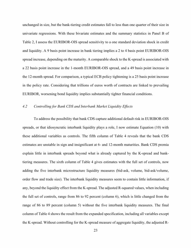
2.1 Sovereign Bond Yield Spreads

Starting with the sovereign bond market, the data sample includes 77 country-maturity

pairs: the government debt securities for 11 euro-area member countries (Austria, Belgium,

Finland, France, Germany, Greece, Ireland, Italy, the Netherlands, Portugal, and Spain) at seven

specific sovereign bond maturity points (1, 2, 3, 4, 5, 7, and 10 years). To precisely compare these

yields, I estimate a smoothed zero-coupon sovereign yield curve, for each maturity m, each country

c, and each day t, by applying the six-parameter model of Svensson (1994) to the prices of all euro-

denominated nominal coupon sovereign debt securities, using bond prices from Bloomberg.9

Figure 1 compares the movements in sovereign bond yields (Equation (1), Panel A) and

yield spreads (Equation (3), Panel B), respectively, for each of the countries in the sample. The

yields mostly decline over the sample, but the yield spreads widen dramatically for several

countries. Figure 1 shows that the five-year spread ranges from -23 to 55 basis points. Other

9 See Gürkaynak, Sack, and Wright (2006) for a discussion of the methodology: http://www.federalreserve.gov/pubs/feds/2006/200628/200628abs.html.

11

horizons show similar widening, as reported in the sovereign bond summary statistics in Table 1.

2.2 Interbank Interest Rate Spreads

In the money market, I consider the 1-, 3-, 6-, and 12-month-maturity EURIBOR-OIS

interest rate spreads. These are EURIBOR maturities commonly referenced in financial contracts.

Panel A of Figure 2 illustrates an even steeper decline in EURIBOR levels than those of sovereign

bonds over the same period (Figure 1, Panel A). The roughly 450 basis point drop in short-term

rates over the sample is largely driven by the ECB’s crisis-driven monetary policy easing in 2008

and 2009, and thus a lower riskfree rate. On the other hand, Panel B shows that the spread between

EURIBOR and OIS rates spikes higher, first in August 2007, and then most dramatically following

Lehman’s Brothers’ bankruptcy in the fall of 2008. The 1-month EURIBOR-OIS spread (which is

always positive) has a standard deviation of 30 basis points, the same as its sample average level,

as shown in Panel A of Table 2. The rise in short-term spreads in 2007 and 2008 received

considerable attention in the press and from policymakers. Widening spreads mean less

accommodative financial conditions ceteris paribus, since many private lending rates are tied to

term interbank rates.10 EURIBOR and OIS rates are obtained from Bloomberg.

2.3 Market Microstructure Liquidity Measures

In order to compare the proposed K-spread liquidity measure with traditional euro-area

sovereign bond liquidity measures, and to allow for country-specific liquidity effects, I obtain

transaction data from MTS, a large electronic European bond trading platform, aggregated to a

10 Swap rates, forward rate agreements, interest rate futures contracts, and many mortgage rates in the euro area reference EURIBOR.

12

daily frequency.11 With these data, I construct five microstructure liquidity measures for each of

the 77 country-maturity pairs: average trade size, total trading volume, the average bid-ask spread,

order flow, and the bid-ask spread scaled by trading volume (Bollen and Whaley (1998) liquidity

index), each aggregated to the daily frequency. Let cmtX be a vector of the five microstructure

liquidity measures for country, c, at maturity m, on day t, and let ' '11

' 1 c m c mtc w X be the sovereign

debt-weighted euro-area average of these liquidity measures at maturity m, where w is the set of

weights used in Equation (2), and c is a counter variable indexing each of the countries. The

microstructure liquidity measure for each country-maturity pair is defined as:

' '

11' 1cmt cmt c m c mtcX X w X (6)

Table 1 reports the country-level summary statistics for the microstructure liquidity

measures, defined as deviations from the weighted average as in Equation (6), showing that each

measure gives a different perspective on liquidity. For instance, the German sample average bid-

ask spread is 7.9 basis points below the euro-area average, at the 10-year maturity, the largest of

all of the country deviations from average. Meanwhile, Italian bonds are traded far more frequently

than those of the other euro-area countries. This suggests that German and Italian bonds enjoy

relatively high liquidity. However, trade sizes are smallest for Italian bonds at each maturity point.

The interbank market uses a parallel set of the five microstructure liquidity measures,

formed directly from unsecured overnight interbank borrowing transactions, data that are

notoriously opaque and difficult to obtain. The measures are denoted mtX , as they are euro-area

aggregates. The transaction data are sourced from e-MID, a large electronic euro-area interbank

11 MTS is an acronym for Mercato dei Titoli di Stato (Market for Sovereign Bonds). MTS is the largest inter-dealer European sovereign bond market platform, comprising an estimated 80 percent of electronic inter-dealer transactions (Euroweek special report, May 2007).

13

trading platform.12 Euro interbank transactions are concentrated at the very shortest maturities;

more than 90 percent of unsecured interbank borrowing is for a horizon of less than one month.13

Because of sparse observations at other horizons, the microstructure measures are formed with

overnight transactions. Table 2 summarizes statistics and correlations among the interbank

microstructure liquidity measures. In Panel B, the average level of the interbank bid-ask spread is

only a few basis points, 4.5. Sample average daily transaction volume captured by the e-MID

platform is €11 billion, and the average trade size is €33 million

2.4 Credit Risk Measures

To identify the credit factor in sovereign bond yields, I collect the sovereign credit default

swap (CDS) premium separately for the 77 country-maturity pairs considered. I treat the CDS

spread as a directly observable credit measure, denoted, cmtd , in Equation (1). I then subtract the

sovereign debt-weighted euro-area average CDS premium from each sovereign CDS premium,

notated as ' '11

' 1cmt c m c mtcd w d in Equation (2), giving cmtd in Equation (3).

Measuring interbank credit risk with bank CDS premia faces the challenge that EURIBOR-

OIS spreads reflect short-horizon risk, while CDS issuance is concentrated at the 5-year maturity.

Very short- (or long-) maturity CDS contracts are less likely to be precise measures of default risk

due to possible liquidity premia, as per Pan and Singleton (2008). Motivated by the default-horizon

mismatch of CDS, I propose a new short-horizon measure of interbank credit risk. The measure is

the dispersion of rates paid by different borrowers in the overnight interbank market, and it is

12 e-MID is an acronym for Elettronica Mercato Interbancario dei Depositi (Electronic Interbank Deposit Market). Transactions on this platform comprise roughly 20 percent of all unsecured euro-denominated interbank transactions over the sample period. 98 percent of the unsecured interbank e-MID sample is comprised of overnight transactions. 13 The ECB’s annual euro money market reports give detailed statistics on borrowing and lending each year. The maturity distribution has consistently shown that the largest share of transactions occurs at the overnight maturity.

14

formed directly from transactions executed on the e-MID trading platform (described earlier in

this section). The use of this credit-tiering indicator is motivated by an assumption that the

dispersion and level of credit risk are proportional. This idea has been used by several researchers

to explain events in the financial crisis. For example, Heider, Hoerova, and Holthausen (2015)

model this relationship specifically in interbank markets. Gorton and Ordoñoz (2014) use variation

in the cross section of stock returns as a proxy for the level of perceived collateral value. The

proposed bank-tiering measure is the baseline credit factor representation, mtd in Equation (5).

Appendix I describes the bank-tiering measure and its construction in detail.

For comparison with the bank-tiering measure, I also consider bank CDS premia. In order

to precisely capture the credit risk that is impounded in EURIBOR, I obtain the 1-year CDS premia

for each EURIBOR participant bank.14 Then, I use the simple average of these banks’ CDS premia

on each day. All CDS data are obtained from Markit. Figure 4 illustrates a large spike in both

measures of bank credit over the sample. However the bank-tiering measure reaches its highest

level in the fall of 2008 (Panel A), whereas the bank CDS premium peaks in early 2009 (Panel B).

3. Credit versus Liquidity in Euro-Area Sovereign Bond Spreads

This section describes the proposed liquidity measure, and then uses it to empirically

determine whether – and to what extent – credit and liquidity potentially drive the unprecedented

cross-sectional variation in euro-area sovereign yield spreads during the sample period.

14 EURIBOR is a trimmed arithmetic average of interbank survey rates collected from a particular set of banks. The 22 EURIBOR survey banks are: Banco Bilbao Vizcaya Argentaria (BBVA), Banco Santander SA, Barclays, Bank of Tokyo Mitsubishi, BNP Paribas, Caiza General de Depositos, Citibank, Credit Agricole, Credit Suisse First Boston (CSFB), Danske Bank, Deutsche Bank, DZ Bank, HSBC, ING, Intesa San Paolo, JP Morgan Chase, Mizuho, Monte dei Paschi di Siena, Lloyds, National Bank of Greece, Natixis, Nordea, Pohjola, Rabobank, Royal Bank of Scotland, Societe Generale, and Unicredit. I do not trim the bank CDS premia before averaging them, because it is not clear that the same banks would be trimmed from the EURIBOR survey as those trimmed according to the distribution of bank CDS premia.

15

3.1 The K-spread Measure of Market Liquidity

Market liquidity is the premium demanded for buying or selling a large quantity of an asset,

such as a sovereign bond, with immediacy.15 Measuring this empirically is challenging. To identify

the liquidity component of euro-area interest rate spreads, I form a new measure of market liquidity

that is constructed entirely from observed bond prices. Identification is not limited to any single

model of liquidity frictions (e.g. asymmetric information). The measure reflects all information

impounded in bond yields, including forward-looking information about future liquidity

conditions, which is a potentially large dimension of liquidity not captured by market

microstructure or transaction-based liquidity measures. Credit and asset characteristics are entirely

controlled for by the nature of the measure’s construction, as described below.

The new measure compares the yields of German government bonds with German agency

bonds, at specific maturities. German government bonds are highly liquid euro-area securities,

backed by the full faith and credit of the German federal government. Their less-liquid counterparts

are bonds issued by the German federal government-owned development bank, KfW, which was

founded in 1948 to facilitate post-war reconstruction. A key feature of the KfW agency bonds,

which safeguards the new liquidity measure against any credit effects, is that the German federal

government has an explicit iron-clad guarantee – written into the German constitution – for all of

KfW’s current and future obligations, equally and without any difference in priority relative to the

federal government bond issues. Since default risk is identical for the two categories of bonds,

market liquidity is the only substantive difference reflected in their yield spread. KfW and federal

15 An important but conceptually distinct type of liquidity is funding liquidity, an institution’s precautionary demand for term funding so as to have liquid assets on its balance sheet. In the interbank market, precautionary demand for funding is closely tied to market participant’s creditworthiness. Credit and funding liquidity are thus particularly hard to disentangle and I do not attempt to do so; in this paper, credit incorporates both default risk and associated funding liquidity.

16

government bonds also have identical tax treatment (Germany does not have a class of tax-exempt

bonds as in the U.S.), and both classes of bonds have an identical zero risk weight for determining

Basel II capital ratios.

To precisely compare the two classes of German yields, I first estimate a smoothed zero-

coupon yield curve for the KfW bonds, on each day, using the same methodology as described for

the sovereign yield curves in subsection 2.1. I then take the zero-coupon yield spread between the

KfW bond and the corresponding German federal government bond at each of the seven maturity

points considered. The m-year K-spread is defined as:

,mt mt Germany mtKfW Y (7)

where mtKfW and ,Germany mtY denote the m-year zero-coupon yields for the KfW agency and German

government bonds, respectively. The K-spread, denoted mt in Equations (1) through (5), is treated

as a directly observable liquidity measure. Its identifying assumption is that German sovereign and

KfW yields have identical credit but that they load differently on the common liquidity factor.

Time series variation in interest rates that comes from market liquidity will load on the K-spread,

but variation due to default will not. Hence, the spread between KfW and German sovereign yields

allows for recovery of that liquidity factor.

Panel A of Figure 3 plots the K-spread for the 1- and 5-year maturities over the sample.

The spread is always positive, reflecting the relative ease with which the federal government debt

is traded as compared to the agency debt. The measure rises most substantially in the second half

of the sample, reaching a local peak of 47 basis points around the collapse of Bear Stearns in March

2008, at the 5-year maturity, and a global peak of 90 basis points following Lehman Brothers’

bankruptcy in the fall of 2008.

There are some institutional differences between KfW and German federal government

17

bonds that could contribute to their liquidity differential. Although they share the same

creditworthiness, the KfW and German federal government bonds are not fungible, even in the

absence of any difference in characteristics. For instance, there is an active futures market for

German 2-, 5- and 10-year federal government bonds, but the comparable-maturity KfW securities

cannot be delivered into these futures contracts.16 Federal government bond issuance is also larger

and trading volume is higher than for KfW securities.17 Moreover, euro repo funding rates are

consistently slightly higher for KfW collateral than for German federal government collateral,

reflecting the relative attractiveness of the federal government securities as collateral in funding

markets.18 The financing rate differential could be both a cause and a consequence of their greater

liquidity (Brunnermeier and Pedersen (2009) and Gorton and Metrick (2012)). The K-spread is

similar in spirit to the measure proposed by Longstaff (2004), who uses the yield spread between

Refcorp (Resolution Funding Corporation) and U.S. Treasury bonds to proxy liquidity premia in

U.S. Treasury markets. But, the K-spread is constructed in the euro-area market, and I directly

apply it to quantify the aggregate bond market liquidity effects in different euro-area country bond

yields and interbank rates.

3.2 The Independent Component of Credit versus Liquidity in Yield Spreads

To investigate the drivers of sovereign yield spreads, I match each of the seven sovereign

16 The existence of futures markets enhances the liquidity of Treasury securities in the U.S. (Fleming (1997), allowing an investor to hedge a position in the underlying security. 17 In 2008, gross annual issuance was €216 billion in federal government debt versus €74 billion for KfW, and the size of government debt was about 8 times that of KfW agency debt. Issue sizes outstanding at the time were around €20 billion for benchmark federal debt issues versus €5 billion for benchmark KfW issues. Nonetheless, KfW is the 4th largest euro-area debt issuer by volume, after the sovereigns of Germany, France and Italy. Trading volume for the federal government debt is roughly 10 times higher than that of the agency market (a daily average of €443 million versus €42 million, respectively), on the MTS platform, over the sample period. 18 KfW bonds may not be used as collateral in federal government repo agreements and vice versa. However, both securities are actively used for funding purposes; they each have centrally cleared general collateral repo markets, and the settlement convention is the same: three days following trade execution (t+3).

18

maturities with the corresponding-maturity K-spread; the 2-year Italian yield spread is

decomposed with the 2-year K-spread, and so on. Similarly, I match the sovereign CDS spread

maturities, and since the CDS are also country-specific, I additionally match these for each country

in the sample. At each maturity point, Equation (3) is then fit as a separate seemingly unrelated

regression (SUR). This allows for the restriction that 2m is the same across countries, and

accounts for contemporaneous cross-equation error correlation. The coefficient 1cm represents the

intertemporal sensitivity of sovereign yield spreads to a common euro-area liquidity factor, directly

measured by the K-spread, for each of the 77 country-maturity pairs. The coefficient 2m measures

the common loading across different country default premia, measured by country CDS spreads,

at each of the seven maturities. An increase in the K-spread or the sovereign CDS spread means a

deterioration in liquidity and credit, respectively.

Table 3 reports the sovereign bond spread estimation at the 2-, 5-, and 10-year maturities

in Panels A, B and C, respectively, with the univariate results in the first four columns of each

panel.19 Market liquidity and credit are independently significantly related to sovereign yield

spreads at each maturity. The estimates for the regressions onto the K-spread alone are highly

significant for 31 out of 33 country-maturity pairs, and a test of the hypothesis that 1 0cm for all

countries jointly is strongly rejected, supporting the idea that the measure identifies commonality

in liquidity.

In a joint regression of sovereign yield spreads onto credit and liquidity together, both

variables remain highly significant (Column 5), giving additional evidence that these two variables

are independently important. Further, an average of the adjusted R-squared values by maturity in

19 Results across the other eight maturities are similar, and detailed in a web appendix (http://finance.wharton.upenn.edu/~kschwarz/Mind%20the%20Gap%20Web%20Appendix.pdf).

19

Column 6, shows that credit and liquidity together explain 80 to 85 percent of the variation in

sovereign bond yield spreads. This is substantially more than is explained by either variable alone.

For liquidity, the average univariate R-squared values range from 61 to 68 percent, depending on

the maturity, and for credit, the univariate R-squared values range from 21 to 40 percent.

3.3 The Relative Role of the K-spread versus Sovereign CDS Spreads

To assess each country’s relative sensitivity to liquidity versus credit, I consider the change

in the sovereign bond yield spread associated with a one standard deviation shock to liquidity and

a comparable shock to credit, using the coefficients estimated jointly in Column 5 of Table 3. The

bond summary statistics in Table 1 are used for calibration; a one standard deviation deterioration

in market liquidity corresponds to an 18 to 25 basis point increase in the K-spread (Panel C),

depending on the maturity, and a comparable credit shock corresponds to a 5 to 66 basis point

increase in the CDS spread (Panel A), depending on the country-maturity combination. Figure 5

summarizes these responses, comparing each country’s yield spread sensitivity in basis points,

averaged over maturities, to a one standard deviation credit (x axis) versus liquidity (y axis)

worsening.

For countries in the upper right quadrant of Figure 5, such as Greece and Ireland, a negative

shock to either credit or liquidity is associated with a higher spread. For those in the lower right

quadrant, a negative liquidity shock has a spread-narrowing effect. German sovereign spreads

show the greatest benefit from worsening liquidity, narrowing by 13 basis points, on average. In

comparison, a one standard deviation deterioration in credit widens average German spreads by

only 5 basis points. So, a concurrent and comparable deterioration in credit and liquidity would

leave German sovereign spreads narrower on net, by 8 basis points. This dynamic is suggestive of

a liquidity feedback effect in the euro-area sovereign debt market, whereby the most liquid

20

securities become more liquid and conversely for the least liquid securities (Amihud and

Mendelson (1986), Dow (2004), Musto, Nini, and Schwarz (2017)). It is also consistent with

Germany’s anecdotal reputation as a euro-area liquidity haven, similar to the documented liquidity

concentration in on-the-run U.S. Treasury securities (Krishnamurthy, 2002).

The two countries furthest from the origin in Figure 5 are clearly Greece and Ireland,

showing the largest absolute sensitivity to both types of shocks. Irish bond sensitivity tilts toward

credit, which may not be surprising since the Irish government explicitly raised its default risk by

guaranteeing the debt of its private banks in 2008 to prevent their collapse. A country close to the

default boundary would naturally be sensitive to further credit shocks. Greek bonds, on the other

hand, are more than twice as sensitive to liquidity as compared to credit, on average. The Greek

debt crisis had not yet taken hold during the sample period, though Greece’s fiscal position was

already the weakest in the euro area.

3.4 Controlling for Country-Specific Liquidity

To compare the K-spread with traditional liquidity measures, and to addresses the potential

concern that a measure with German origins may not fully capture other countries’ liquidity

effects, Equation (3) is now expanded to contain the five country-specific market microstructure

liquidity measures cmtX , as defined in Section 2:

1 2 3cmt cm mt m cmt cmtm cmty d X (9)

The coefficient 3m measures yield spread sensitivity to the additional liquidity measures at each

maturity point. For two of the microstructure measures, the bid-ask spread and the Bollen-Whaley

index, a higher value indicates deteriorating liquidity. For the remaining three measures (volume,

trade size and order flow), a higher value denotes improving liquidity.

21

The two right-most columns of Table 3 show the expanded SUR results. A joint hypothesis

test of the null that 3 0m , for all five market microstructure liquidity measures, is strongly

rejected. However, no single microstructure measure is significant at all maturities, and the

estimates are unstable in sign, except for trade size. The country CDS and the K-spread estimates

remain highly significant and remarkably close to their values in the bivariate case. A comparison

of the R-squared values for the different specifications shows little incremental benefit to adding

the microstructure measures; averaged across countries and maturities, the adjusted R-squared is

83 percent with only sovereign CDS and the K-spread as explanatory variables, compared to 85

percent with the full specification.

The relatively small role for microstructure measures of liquidity is consistent with Beber,

Brandt and Kavajecz (2009), who found that credit (measured with sovereign CDS spreads) was

far more important than microstructure liquidity variables for euro-area sovereign yields over 2003

and 2004. In a calibration of the estimates from Equation (9) with the summary statistics in Table

1, a one standard deviation shock to the microstructure liquidity measures is associated with an

average of less than 1 basis point change in sovereign yield spreads. Despite the empirical

advantage of the microstructure measures in relating distinctly to each country’s sovereign bond

yield spreads, the K-spread and CDS remain paramount in explaining sovereign spreads. Section

5 sheds light on the nature of the liquidity effect – does it represent the manifestation of poor

liquidity or the risk of worsening liquidity?

4. The Role of Aggregate Bond Market Liquidity in Euro-Area Interbank Spreads

The models of Brunnermeier and Pedersen (2009) and Bolton, Santos and Scheinkman

(2011) describe a close relationship between bond and funding markets. This section empirically

22

assesses the effect of aggregate bond liquidity in the funding market by using the K-spread to parse

interbank rates.

4.1 Aggregate Bond Market Liquidity and Bank-Tiering Credit in Interbank Interest Rates

To estimate risk effects in euro-area interbank rates, I conduct a time-series regression

corresponding to the framework set out in Equation (5). The specification is:

1 2 3 4cds

mt m t m t m t m t mty d d X (10)

where mty denotes the EURIBOR minus OIS spread at maturity m on day t, t is the K-Spread

measure of euro-area sovereign bond market liquidity20, td is the bank-tiering measure of credit

risk, cdstd is the average EURIBOR bank CDS premium and tX is a vector containing the interbank

market microstructure liquidity measures. Separate regressions are run for the 1-, 3-, 6- and 12-

month EURIBOR-OIS maturities.

Table 4 shows the estimation results for Equation (10) in Panels A through D, at each of

the four maturity points. Univariate regression estimates, reported in the first three columns of

each panel, show that the K-spread, the bank-tiering credit measure, and the bank CDS premia, are

each independently significant at the 1 percent level. The estimates are all positive, consistent with

the intuition that a deterioration in either credit or aggregate market liquidity conditions would

lead banks to charge one another a higher borrowing premium.

The fourth column of each panel in Table 4 shows the joint effect of credit and liquidity,

estimated with a regression of EURIBOR-OIS spreads onto both the K-spread and the bank-tiering

credit measure. In comparison to the univariate case, the K-spread coefficient estimates are nearly

20 Results are reported when using the one-year maturity K-spread measure for the analysis of interbank spreads, but the estimation is not sensitive to the choice of maturity.

23

unchanged in size, but the bank-tiering credit estimates fall to less than one quarter of their size in

univariate regressions. With these bivariate estimates and the summary statistics in Panel B of

Table 2, I assess the EURIBOR-OIS spread sensitivity to a one standard deviation shock in credit

and liquidity. A 9 basis point increase in bank tiering implies a 2 to 4 basis point EURIBOR-OIS

spread increase, depending on the maturity. A comparable shock to the K-spread is associated with

a 22 basis point increase in the 1-month EURIBOR-OIS spread, and a 49 basis point increase in

the 12-month spread. For comparison, a typical ECB policy tightening is a 25 basis point increase

in the policy rate. Considering that trillions of euros worth of contracts are linked to prevailing

EURIBOR, worsening bond liquidity implies substantially tighter financial conditions.

4.2 Controlling for Bank CDS and Interbank Market Liquidity Effects

To address the possibility that bank CDS capture additional default risk in EURIBOR-OIS

spreads, or that idiosyncratic interbank liquidity plays a role, I now estimate Equation (10) with

these additional variables as controls. The fifth column of Table 4 reveals that the bank CDS

estimates are unstable in sign and insignificant at 6- and 12-month maturities. Bank CDS premia

explain little in interbank spreads beyond what is already captured by the K-spread and bank-

tiering measures. The sixth column of Table 4 gives estimates with the full set of controls, now

adding the five interbank microstructure liquidity measures (bid-ask, volume, bid-ask/volume,

order flow and trade size). The interbank liquidity measures seem to contain little information, if

any, beyond the liquidity effect from the K-spread. The adjusted R-squared values, when including

the full set of controls, range from 86 to 92 percent (column 6), which is little changed from the

range of 86 to 89 percent (column 5) without the five interbank liquidity measures. The final

column of Table 4 shows the result from the expanded specification, including all variables except

the K-spread. Without controlling for the K-spread measure of aggregate liquidity, the adjusted R-

24

Squared value falls by more than one-quarter (column 7).

The estimation results in Table 4 suggest that steps to improve market liquidity could

narrow interbank spreads substantially, independent of any credit effect. In the fall of 2008,

EURIBOR-OIS spreads rose from less than 10 basis points to 150 and 240 basis points at the 1-

and 12-month maturities, respectively. Now, consider an extreme hypothetical counterfactual

scenario in which all assets are made equally liquid. The K-spread would then be zero (below even

the small positive spread prior to the crisis). Judging from the bivariate regression results in the

fourth column of Table 4, this would narrow the sample average EURIBOR-OIS spread to 6 basis

points at the 1-month maturity and 20 basis points at the 12-month maturity, closely approximating

the narrowness of pre-crisis interbank spreads (illustrated in Figure 2, Panel B).21 The other

regression specifications give similar implications.

The relatively small role for credit risk in the euro-area interbank market may seem

surprising at first, but it could partly stem from a belief that government intervention would prevent

near-term bank defaults, especially for the large banks that comprise the EURIBOR survey.

Beginning in August 2007, U.S. and European central banks took many operational measures to

target general funding pressures.22 Though such measures may mitigate default risk in the short

run, they could exacerbate risk in the long run if the extraordinary measures taken are not

sustainable. The importance of liquidity in interbank spreads is broadly consistent with the results

21 The sample average EURIBOR-OIS spread is 30.4 and 75.1 basis points at the 1- and 12-month maturities, respectively (Table 2, Panel A), and the K-spread is 26.4 basis points on average over the sample (Table 2, Panel B). At the 1-month maturity, the K-spread equal to 0 implies a decline in the 1-month EURIBOR-OIS spread to 0.94×26.4=24.8 basis points, and 2.08×26.4=54.9 basis points at the 12-month maturity. Subtracting these from the sample-average OIS spreads gives 1- and 12-month EURIBOR-OIS spreads of 30.4-24.8=6 and 75.1-54.9=20 basis points, respectively. 22 These measures include massive overnight funds injections, loosening the terms of standard funds injections (such as accepting a broader range of collateral), relaxing the terms of emergency lending facilities (such as widening the base of eligible counterparties), and introducing new dollar swap, term funds lending, and securities lending facilities. See Brunnermeier (2009) for a detailed account of liquidity and credit events over this period.

25

of Gefang, Koop and Potter (2011) who find that a liquidity factor helps explain much of the

variation in a panel dataset of LIBOR-OIS spreads. The large role for the K-spread suggests that

it may capture a channel that is missed by the other liquidity measures considered. The pricing of

liquidity risk will be directly tested for in the next section.

5. Pricing Liquidity Risk

Liquidity risk, defined as the covariance of sovereign bond returns with changes in market

liquidity, is a forward-looking manifestation of market liquidity. Liquidity characteristics, such as

trading volume, or model-based measures, such as the bid-ask spread, gauge prevailing market

conditions. To the extent that the liquidity risk dimension matters, the effect of liquidity captured

by instantaneous measures alone will be underestimated. The liquidity risk channel could help to

explain the relatively small role for the traditional microstructure liquidity measures in euro-area

interest rate spreads, as compared to the proposed K-spread liquidity measure that contains the risk

information embedded in bond yields (Sections 3 and 4).

5.2 Estimating Each Country’s Bond Return Sensitivity to Liquidity

The rich cross section of bond returns across countries and maturities in the euro-area is an

ideal setting in which to directly test the pricing of liquidity risk.23 I employ a two-step Fama

MacBeth procedure to estimate liquidity risk premia. In the first step of the estimation, I assess the

factor sensitivity of each country’s sovereign bonds to changes in the K-spread by running a

separate time series regression for each country-maturity combination, as follows:24

1 1( )Liq

cmt cmt cm cm mt mt cmty y (11)

23 The EURIBOR-OIS spread does not have the same cross-country variation needed for liquidity risk identification. 24 The excess return is approximately the negative change in yield, multiplied by the duration.

26

where 1cmt cmty y denotes the change in the country-maturity yield spread, relative to the

corresponding 11-country average, from day t-1 to day t, and 1mt mt denotes the corresponding

change in the K-spread. I estimate Liqcm for each of the 77 country-maturity pairs, which identifies

each country-maturity pair’s sensitivity in sovereign bond returns to changes in aggregate market

liquidity. An asset with a negative Liqcm is a good hedge because it has high returns (narrowing

yield spreads) when liquidity worsens, whereas an asset with a very positive Liqcm has relatively

low returns when aggregate liquidity deteriorates. The Liqcm estimates range from -0.31 for

Germany to 0.38 for Greece, both at the 5-year maturity, and the standard deviation of Liqcm is 0.17.

Variation in Liqcm helps to precisely identify the price of liquidity risk in the next stage.

5.1 A Systematic Relationship Between Country Sensitivity to Liquidity and Yield Spreads

In the second stage of the Fama MacBeth procedure, I relate the cross-sectional variation

in Liqcm to the cross section of average yield spreads. In this step, to control for effects that are

separate from liquidity risk, I include the sovereign CDS spreads and microstructure liquidity

measures as considered in the sovereign decomposition in Section 3. The second stage cross-

sectional regression is:

0 1 2

ˆ Liqcm c m ccm my X (12)

where cmy is the sample average sovereign yield spread (relative to the euro-area average) for

country c, at maturity m, ˆ Liqcm is the coefficient estimate on the K-spread in the time series

regression from Equation (11), and cmX represents the CDS and microstructure liquidity

27

controls.25 In this regression, 1 gives the market pricing of liquidity risk and 2 gives the direct

effects of CDS spreads and liquidity characteristics on yield spreads. In the context of the liquidity

controls, the coefficients 1 and 2 can be thought of as a liquidity factor and a liquidity

characteristic, respectively, in the terminology of Daniel and Titman (1997).

The results in Table 5 show that liquidity risk is priced in sovereign bond markets, with or

without including the control variables. The coefficient estimate, 1 , is highly significant and

positive, in all specifications, reflecting the premium demanded by investors for the risk that bonds

will become less liquid in the future. An investor demands a higher yield on bonds that are risky

in the sense of offering lower returns when aggregate liquidity is poor. The coefficient estimate on

sovereign CDS spreads, 2 , shown in the second and third columns of Table 5, is also highly

significant and positive, consistent with the important role shown for credit in the sovereign yield

spread estimation in Section 3. However, the incremental role of liquidity characteristics, as

represented by the microstructure liquidity variables, is small once controlling for liquidity betas.

The adjusted R-squared value from a regression onto ˆ Liqcm and CDS alone is 87 percent, and this

increases to 89 percent when including all of the liquidity characteristics.

Using the second stage regression estimates that include all controls (column 3 of Table 5),

Figure 7 plots the average basis point effect of liquidity risk priced into country sovereign bond

yield spreads, by maturity. Perhaps unsurprisingly, liquidity risk tends to play the smallest role in

short-maturity bonds. German bonds benefit more from their potential to hedge worsening

liquidity than any of the other euro-area country bonds. Because of this, German yields are 12

basis points lower on average over the sample. Italian and Greek sovereign bonds, on the other

25 The strategy is similar in spirit to Calomiris, Love, and Peria (2012), who consider a cross-sectional regression of firms’ average stock returns onto their time series betas with respect to crisis shocks.

28

hand, show sample average yields that are 13 and 14 basis points higher, respectively, due to

liquidity risk premia. These bonds suffer most from the perceived risk of low returns in times of

poor liquidity.

The results in this section evidence the large role of liquidity risk premia in euro-area yields

over the crisis period, a channel of market liquidity that is not captured by traditional measures.

6. Conclusion

Beginning in August 2007, interest rate spreads across markets widened dramatically,

threatening the stability of the financial system and the broader economy. There are two primary

factors behind these movements: (1) a higher likelihood of default, and (2) market liquidity effects,

separate from default risk. Policy prescriptions for addressing risk conditions differ, depending on

the primary driver of interest rate spread widening. If the chief component is default, then only

actions to improve the solvency of the issuer are likely to be successful. On the other hand, if the

main driver is market liquidity, then measures to improve market functioning are the most

appropriate. From a practitioner standpoint, a disruption to market liquidity may represent an

attractive opportunity for a long-horizon investor to exploit, whereas deteriorating credit risk

would not.

The first contribution of this paper is to construct a new measure of market liquidity from

asset prices that does not rely on any single model of market liquidity. The measure is the

difference in yields between two bonds that have identical credit risk but differing market liquidity:

German KfW-agency bonds and their federal government counterparts. This spread, the K-spread

liquidity measure, recovers all information in bond yields that is not related to default risk.

Second, the K-spread liquidity measures is used to estimate the precise contribution of

credit and market liquidity risks, independent from one another, in explaining euro-area sovereign

29

bond and EURIBOR-OIS spreads during the 2007-2009 financial crisis. The K-spread shows a

substantially larger role for market liquidity than traditional microstructure measures.

Additionally, relating the K-spread measure to interbank rates gives empirical evidence of the large

and significant influence of aggregate bond market liquidity on interbank rates, supporting the idea

of a general equilibrium relationship between asset markets and funding markets.

Finally, through dispersion in return sensitivities over time, countries and maturities, I find

large and highly significant liquidity factor risk premia in bonds over the crisis sample period.

These risk premia represent compensation demanded by investors for the possibility that liquidity

will worsen in the future at precisely the time when they most want to transact. The K-spread

liquidity measure includes this liquidity risk channel because of its construction from forward-

looking bond yields. In contrast, transaction-based measures of instantaneous liquidity will tend

to understate the contribution of liquidity to interest rates by missing liquidity risk premia. This

underestimation is most critical in times of market stress when risk premia play an important role.

The results in this paper have implications for policymakers and for the portfolio choices

of investors. For practitioners, a long/short position mimicking the K-spread can hedge against

credit fluctuations. The measure itself can gauge real-time pricing of market liquidity risk, helping

to inform investment decisions. For policymakers, the results imply that measures to improve

market functioning, or even an action that addresses risk perceptions alone, could be effective in

bringing down risk spreads. Importantly, such measures can help to avoid the risk of an adverse

feedback loop between the liquidity of asset markets and the liquidity of funding markets, and in

turn the state of the economy.

30

REFERENCES

Acharya, Viral V. and Lasse H. Pedersen, 2005, Asset Pricing with Liquidity Risk, Journal of

Financial Economics, 77: 375-410. Acharya, Viral V. and David Skeie, 2011, A Model of Liquidity Hoarding and Term Premia in

Inter-Bank Markets, Journal of Monetary Economics, 58 (5): 436-447. Afonso, Gara, Anna Kovner and Antoinette Schoar, 2011, Stressed Not Frozen: The Federal Funds

Market in the Financial Crisis, Journal of Finance, 66 (4): 1109-1139. Amihud, Yakov and Haim Mendelson, 1986, Asset Pricing and the Bid-Ask Spread, Journal of

Financial Economics, 17: 223-249. Bao, Jack, Jun Pan and Jiang Wang, 2011, The Illiquidity of Corporate Bonds, Journal of Finance,

66 (3): 911-946. Beber, Alessandro, Brandt, Michael W. and Kavajecz, Kenneth A., 2009, Flight-to-Quality or

Flight-to-Liquidity? Evidence from the Euro-Area Bond Market, Review of Financial Studies, 22: 925-957.

Bollen, Nicholas P.B. and Robert E. Whaley, 1998, Are Teenies Better? Journal of Portfolio

Management, 25: 10-24. Bolton, Patrick, Santos, Tano and Jose A. Scheinkman, 2011, Outside and Inside Liquidity,

Quarterly Journal of Economics, 126(1): 259-321. Bongaerts, Dion, Frank de Jong and Joost Driessen, 2013, An Asset Pricing Approach to Liquidity

Effects in Corporate Bond Markets, Working Paper. Bongaerts, Dion, Frank de Jong and Joost Driessen, 2011, Derivative Pricing with Liquidity Risk:

Theory and Evidence from the Credit Default Swap Market, Journal of Finance, 66 (1): 203-240.

Brunnermeier, Markus K., 2009, Deciphering the 2007-08 Liquidity and Credit Crunch, Journal

of Economic Perspectives, 23: 77-100. Brunnermeier, Markus K. and Lasse H. Pedersen, 2009, Market Liquidity and Funding Liquidity,

Review of Financial Studies, 22: 2201-2238. Calomaris, Charles W., Inessa Love and Maria Soledad Martinez Peria, 2012, Stock returns’

sensitivities to crisis shocks: Evidence from developed and emerging markets, Journal of International Money and Finance, 31: 743-765.

Chordia, Tarun, Sarkar, Asani and Avanidhar Subrahmanyam, 2005, An Empirical Analysis of

31

Stock and Bond Market Liquidity, Review of Financial Studies, 18: 85-129. Daniel, Kent and Sheridan Titman, 1997, Evidence on the Characteristics of Cross-Sectional

Variation in Stock Returns, 52(1): 1-33. Dick-Nielsen, Jens, Peter Feldhütter and David Lando, 2012, Corporate Bond Liquidity Before

and After the Onset of the Subprime Crisis, Journal of Financial Economics, 103 (3): 471-492.

Dow, James 2004. Is Liquidity Self‐Fulfilling? The Journal of Business, 77(4), 895-908. Ehrmann, Michael, Marcel Fratzscher, Refet S. Gürkaynak and Eric T. Swanson, 2011,

Convergence and Anchoring of Yield Curves in the Euro Area, Review of Economics and Statistics, 93 (1): 350-364.

Favero, Carlo, Marco Pagano and Ernst-Ludwig von Thadden, 2010, How Does Liquidity Affect

Sovereign Bond Yields, Journal of Financial and Quantitative Analysis, 45: 107-134. Filipović, Damir and Anders B. Trolle, 2013, The Term Structure of Interbank Risk, Journal of

Financial Economics, 109 (3): 707-733. Fleming, Michael J., 1997, The Round-the-Clock Market for U.S. Treasury Securities, Economic

Policy Review, 3: 9-32. Friewald, Nils, Rainer Jankowitsch and Marti G. Subrahmanyam, 2012, Illiquidity or Credit

Deterioration: A Study of Liquidity in the U.S. Corporate Bond Market during Financial Crises, Journal of Financial Economics, 105: 18-36.

Gefang, Deborah, Gary Koop and Simon Potter, 2011, Understanding Liquidity and Credit Risks

in the Financial Crisis, Journal of Empirical Finance, 18: 903-914. Gorton, Gary and Andrew Metrick, 2012, Securitized Banking and the Run on Repo, Journal of

Financial Economics, 104 (3): 425-451. Gorton, Gary, Andrew Metrick and Lei Xie, 2015, The Flight from Maturity, NBER Working

Paper, 20027. Gorton, Gary and Guillermo Ordoñez, 2014, Collateral Crises, American Economic Review, 104

(2): 343-378. Gürkaynak, Refet S., Brian Sack and Jonathan H. Wright, 2006, The U.S. Treasury Yield Curve:

1961 to the Present, Finance and Economics Discussion Series 2006-28. Heider, Florian and Marie Hoerova, 2009, Interbank Lending, Credit Risk Premia and Collateral,

International Journal of Central Banking, 5: 1-39.

32

Heider, Florian, Marie Hoerova and Cornelia Holthausen, 2015, Liquidity Hoarding and Interbank Market Spreads: The Role of Counterparty Risk, Journal of Financial Economics, forthcoming.

Jankowitsch, Rainer, Hannes Mösenbacher and Stefan Pichler, 2006, Measuring the Liquidity

Impact on EMU Sovereign Bond Prices, European Journal of Finance, 12: 153-169. Kuo, Dennis, David Skeie and James Vickery, 2012, A Comparison of LIBOR to Other Measures

of Bank Borrowing Costs, Federal Reserve Bank of New York Working Paper. Krishnamurthy, Arvind, 2002. The Bond/Old-Bond Spread. Journal of Financial Economics, 66,

463-506. Lin, Hai, Junbo Wang and Chunchi Wu, 2011, Liquidity Risk and Expected Corporate Bond

Returns, I, 99 (3): 628-650. Longstaff, Francis A., 2004, The Flight-to-Liquidity Premium in U.S. Treasury Bond Prices,

Journal of Business, 77: 511-526. Longstaff, Francis A., 2009, Portfolio Claustrophobia: Asset Pricing in Markets with Illiquid

Assets, American Economic Review, 99 (4): 1119-44. Manganelli, Simone and Guido Wolswijk, 2009, What Drives Spreads in the Euro Area Sovereign

Bond Market? Economic Policy, 24: 191-240. McAndrews, James, Asani Sarkar and Zhenyu Wang, 2008, The Effect of the Term Auction

Facility on the London Inter-Bank Offered Rate, Federal Reserve Bank of New York Staff Report, 335.

Merton, Robert C., 1974, On the Pricing of Corporate Debt, The Risk Structure of Interest Rates,

Journal of Finance, 29: 449-470. Michaud, Francois-Louis and Christian Upper, 2008, What Drives Interbank Rates? Evidence

from the Libor Panel, BIS Quarterly Review: 47-58. Musto, David, Greg Nini and Krista Schwarz, 2015, Notes on Bonds: Liquidity at All Costs in the

Great Recession, Working Paper. Pan, Jun and Kenneth J. Singleton, 2008, Default and Recovery Implicit in the Term Structure of

Sovereign CDS Spreads, Journal of Finance, 63 (5): 2345-2384. Packer, Frank and Naohiko Baba, 2009, From Turmoil to Crisis: Dislocations in the FX Swap

Market before and after the Failure of Lehman Brothers, Journal of International Money and Finance, 28 (8): 1350-1374.

Pastor, Lubos and Robert Stambaugh, 2003, Liquidity Risk and Expected Stock Returns, Journal

33

of Political Economy, 111: 642-685. Shleifer, Andrei and Robert W. Vishny, 1997, The Limits of Arbitrage, Journal of Finance, 52:

35-55. Svensson, Lars E. O., 1994, Estimating and Interpreting Forward Rates: Sweden 1992-4, NBER

Working Paper, 4871. Taylor, John B. and John C. Williams, 2009, A Black Swan in the Money Market, American

Economic Journal, Macroeconomics, 1: 58-83. Vayanos, Dimitri, 2004, Flight to Quality, Flight to Liquidity, and the Pricing of Risk, NBER

Working Paper, 10327.

34

Appendix I

Bank Credit Tiering Measure Estimation

Default risk premia in unsecured interbank interest rates are unobservable, But, the

difference in interbank borrowing rates at the same point in time controls for the common

component and isolates the difference in risk premia between these borrowers.26 The new bank-

tiering credit measure takes the difference between two contemporaneous unsecured borrowing

rates: the daily-average rate paid by banks in the highest quintile of credit and the daily-average

rate paid by banks in the lowest quintile of credit. Considering only the spread between the two

rates removes the common risks and market conditions that are faced by all market participants on

the e-MID platform. The bank-tiering credit measure, td , driven by the relative credit premia of

the two bank types, is defined as follows:

, ,t t High t Lowd r r (13)

where ,t Highr and ,t Lowr denote the average unsecured interbank borrowing rates paid by the banks

in the highest and lowest risk quintiles, respectively, on day t.

To motivate this approach, suppose that the spread between the interest rate that bank

has to pay on day and the hypothetical risk-free interest rate is multiplicative of the form

where is a bank fixed effect and is a time fixed effect. Normalize the average to one and

let the cross-sectional dispersion of be θ. Then the average credit premium on any day is and

the dispersion across banks on any day is . The average credit premium on day t is thus

26 In the unsecured interbank market, the lender is fully exposed to the credit risk of the borrower, and this is the only credit risk that the lender faces. The interbank rate thus prices the likelihood of repayment by the borrower.

j

t j tb r

jb tr jb

jb tr

tr

35

proportional to the dispersion in rates. 27 In this model, as the default risk of low credit institutions

worsens, that of high credit institutions worsens proportionately more, and so an increase in the

average rate difference between these two tiers of borrowers reflects an increase in the overall

level of credit. The intuition is consistent with that of structural credit models. For instance,

Merton’s 1974 model predicts that the credit premium is approximately proportional to rate

volatility. It is also consistent with the idea that credit is largely driven by a systemic factor

(Longstaff, Pan, Pedersen and Singleton (2011)).

To operationalize this bank-tiering measure, I use the unique database of signed interbank

transactions from e-MID, an electronic interbank trading platform. These data show the negotiated

rate and bank identities of the borrower and lender for each individual trade that takes place over

the sample, plus the time stamp, maturity, volume, and the initiating side of each trade.28 There

are two key features of the e-MID platform that are important to the interpretation of the transaction

rates. First, the lender in a trade is fully exposed to the default risk of a borrower in these trades

that are facilitated but not backed by e-MID. This contrasts with trades in centrally cleared markets,

such as futures, where the clearinghouse effectively becomes the counterparty to each trade.

Second, e-MID transactions are identity-transparent; a participant can view all limit orders posted

by platform participants, alongside of their respective bank identities, and can choose to take the

other side of any order that is posted.29 A bank will initiate a market order to lend only if the posted

27 A simple example illustrates the model’s multiplicative assumption. Suppose on a day with low credit and

on a day with high credit, and suppose for the best credit bank and for the worst credit bank.

Then credit tiering on a good credit day would be and credit tiering on a bad credit day would be

. 28 One distinct advantage of the new credit measure is that it is constructed from rates on actual unsecured interbank transactions and thus reflects true borrowing costs, whereas survey-derived rates such as LIBOR may be affected by manipulation. A comparison of LIBOR and other measures of bank borrowing costs is reported in Kuo, Skeie and Vickery (2012). 29 In contrast, the MTS bond trading platform follows conventional price-time priority; trades are matched automatically based on the most attractive quote submitted, with priority given to the earliest submission. The

1tr

5tr 0.5jb 1.5jb

1low worst low bestr b r b 5high worst high bestr b r b

36

borrowing rate sufficiently compensates the lender for the risk of the trade. It follows that the

credit-relevant information on e-MID comes from the rates on limit orders to borrow (or

equivalently market orders to lend), where trades are agreed to with the foreknowledge of the

borrower’s identity.30

I use the rate and borrower identity information in e-MID limit order data to form a bank-

tiering measure of credit, in the following 3 steps.

1. First, to estimate banks’ credit quality, I run the following pooled regression: 31

1 1 1, , , 1 1, 1 2, 1 3, , , ,

m n Th i j t h h h j j j t t t i h j tr T B D

(14)

where , , ,h i j tr denotes the unsecured interbank rate paid by borrower j in its ith transaction on

day t in hour h. denotes the time-of-day indicator variable for each hour, h, denotes the

indicator variable for bank borrower j, and denotes the indicator variable for day t. The day

and time indicators control for effects common to all rates, including interbank market-wide

liquidity shocks.32 The bank dummy coefficient, 2, j , estimates the average credit quality of

each bank.33 Considering only the borrowing side of the quote avoids any contribution of noise

counterparty’s identity is revealed only after the trade is agreed to, which eliminates counterparty risk effects from bond trades on the MTS platform. 30 The intuition behind an identity-transparent platform for interbank markets is that the interbank loan is effectively the equivalent to the traded asset in an asset market. Just as a bond market participant would find it difficult to price a bond without knowing the identity of the bond issuer, an interbank market participant would be reluctant to lend unsecured funds to a mystery borrower. The relationship between counterparty default risk and the credit of an interbank trade is precisely what drives the transparent information structure of the e-MID platform. The importance of the borrower’s identity is evident; 81 percent of interbank lending volume in the sample is via market order. Following the crisis, e-MID introduced a parallel platform where identities were not revealed, but there was very little market interest to transact “confidentially.” 31 Estimation is necessary because each bank in the sample has a unique but generic identifier that does not reveal the bank’s actual identity. A priori, I cannot tell which banks are good/bad credits from their e-MID identifiers alone. 32 Controlling for the day effect in Equation (14) is important as the overall level of rates changed over the sample. The ECB raised its policy rate by 25 basis points on March 14, 2007 and again on June 13, 2007. Another way to isolate the credit component of interbank rates is to subtract the daily GC repo rate from the left-hand side of Equation (14). However, this approach confounds the credit component with repo market seasonality. 33 There is no way to insure against the default of interbank deposits. In principal, a CDS contract could be entered into each day with the counterparty’s debt as the reference obligation, but transactions costs would be prohibitive. In

hT jB

tD

37

to the measure from the bid-ask bounce. I re-estimate the banks’ creditworthiness each day,

using the past 30 days of transactions, updating each banks’ relative ranking based on its most

recent borrowing rates.

2. Next, I sort borrowers into credit quintiles according to their 2, j credit coefficient estimates;

the top quintile represents banks that paid the highest average rates, and are thus perceived as

the worst credits.34 Each quintile contains the same number of banks. For an apples-to-apples

comparison, I use only maturity-matched trades.35 To mitigate any survivorship bias, I only

use rates of banks transacting in both the first and last quarters of the sample, reducing the

bank sample to 135.

In the third and final step, I define the bank-tiering credit measure. Let ,t Highr and ,t Lowr denote

the average rates paid by the banks in the highest and lowest risk quintiles, respectively, on

day t (averaged across all hours on each day). The bank-tiering credit measure is then simply

, ,t High t Lowr r as in equation (13).

Figure 4, Panel A plots the new bank-tiering credit measure, showing that it peaks at 63 basis

points in October 2008. This compares a less-than 5 basis point difference in average rates paid by

the best- versus worst-credit banks in normal times.

practice, these loans are not resold. Novation requests, or third party risk assumption for a transaction, occurred during the crisis. But, this was motivated by risk reduction of outstanding obligations, not to insure new transactions. 34 To check whether I have captured the difference between rates paid by high credit and low credit institutions, I consider the propensity to borrow via limit order versus market order for different credit quintiles. Low credit banks should prefer to borrow via limit order so that their identity is factored into the counterparty’s lending rate; the lending bank will know that the borrower is low risk and will thus agree to a relatively low rate. It turns out that borrowing via market order as a fraction of total borrowing is 92 percent in the best credit quintile, compared to 57 percent in the lowest credit quintile. In fact, the propensity to borrow via limit order is monotonically increasing in credit quintile, supporting the idea that the grouping of banks by quintile has indeed separated the good credit banks from the bad credit banks. 35 In the sample, 91 percent of transaction volume is agreed to for maturity on the following business day. This is comparable to the interbank market as a whole, in which the vast majority of transactions are overnight, to help banks meet day-to-day fluctuations in their funding needs.

38

Table 1. Sovereign Bond Market  

PanelA:SovereignYieldSpreads,SovereignCDSSpreads,andMicrostructureLiquidityMeasures(Deviationsfrom11‐Country€ Average)SovereignYieldSpreadc SovereignCDSc Bid‐AskC VolumeC TradeSizeC OrderFlowC BWIndexC

(bps) (bps) (bps) (€bn) (€mn) (€bn) (ratio)Mean StDev Mean StDev Mean StDev Mean StDev Mean StDev Mean StDev Mean StDev

2‐YearMaturityAustria 1.83 7.09 10.63 23.19 0.29 0.91 ‐0.11 0.09 1.39 1.91 ‐0.01 0.26 0.05 0.21Belgium 4.49 5.26 ‐2.33 4.95 0.75 0.75 ‐0.09 0.09 1.02 2.13 ‐0.08 0.39 0.01 0.30Germany ‐14.97 16.52 ‐12.85 15.34 ‐0.19 0.36 ‐0.07 0.08 ‐0.01 1.88 0.02 0.18 0.08 0.26Spain 5.07 6.76 5.96 6.69 0.62 0.64 ‐0.10 0.08 1.07 2.52 0.00 0.26 0.05 0.22Finland ‐7.42 7.62 ‐11.98 14.37 ‐0.28 1.02 ‐0.12 0.09 ‐0.60 2.76 0.00 0.21 0.18 0.31France ‐7.50 9.34 ‐11.63 13.60 0.39 0.52 ‐0.08 0.08 0.62 2.13 ‐0.04 0.21 0.03 0.21Greece 42.60 47.52 32.90 40.47 0.29 0.93 ‐0.11 0.08 ‐0.69 2.37 0.02 0.22 0.11 0.28Ireland 17.14 33.27 44.74 65.60 ‐0.75 1.09 ‐0.12 0.09 1.40 2.06 0.14 0.20 ‐0.09 0.21Italy 14.54 16.37 15.35 18.15 ‐0.55 0.37 0.26 0.20 ‐2.02 1.30 0.02 0.24 ‐0.13 0.15Netherlands ‐9.75 10.48 ‐4.77 4.63 0.01 0.62 ‐0.09 0.14 2.39 4.74 0.03 0.63 ‐0.03 0.20Portugal 14.00 13.73 4.39 5.57 ‐0.34 1.21 ‐0.07 0.09 1.24 1.81 0.02 0.44 ‐0.11 0.21

5‐YearMaturityAustria 1.25 7.48 10.00 26.10 0.47 2.20 ‐0.05 0.07 0.90 2.33 ‐0.03 0.25 0.09 0.74Belgium 7.33 7.99 ‐2.31 4.86 1.38 1.38 ‐0.01 0.08 0.55 1.96 ‐0.05 0.28 0.05 0.72Germany ‐23.37 22.26 ‐17.68 17.07 ‐2.18 1.70 ‐0.04 0.06 ‐0.55 1.81 0.00 0.17 0.07 0.64Spain 4.33 7.16 10.17 8.26 1.26 2.40 ‐0.03 0.07 1.16 2.44 0.02 0.24 0.09 0.96Finland ‐3.34 4.24 ‐16.35 15.65 ‐0.15 2.08 ‐0.03 0.07 1.65 1.80 ‐0.12 0.36 ‐0.12 0.56France ‐8.52 9.74 ‐14.88 14.77 1.26 1.20 ‐0.04 0.06 ‐0.20 1.90 ‐0.01 0.16 0.15 0.60Greece 54.94 59.45 41.69 43.41 0.41 1.84 ‐0.04 0.06 ‐0.42 2.01 0.00 0.16 0.20 0.68Ireland 35.76 54.79 44.41 63.10 ‐0.44 1.78 ‐0.05 0.06 0.73 2.47 ‐0.01 0.27 ‐0.24 0.56Italy 15.66 13.41 21.09 18.96 ‐0.74 1.25 0.16 0.19 ‐1.60 1.14 0.03 0.31 ‐0.27 0.46Netherlands ‐4.29 3.76 ‐9.20 6.46 ‐0.64 1.97 ‐0.03 0.12 2.35 2.64 0.04 0.51 ‐0.17 0.52Portugal 16.09 15.69 7.32 6.73 0.52 2.14 ‐0.01 0.09 1.12 2.03 0.01 0.36 ‐0.14 0.47

10‐YearMaturityAustria ‐2.36 6.47 5.55 23.04 ‐0.16 3.79 ‐0.03 0.06 1.18 2.35 ‐0.02 0.22 ‐0.38 1.46Belgium ‐0.29 4.48 ‐5.13 6.45 1.30 3.97 ‐0.03 0.06 2.15 2.13 0.04 0.23 ‐0.27 1.37Germany ‐26.76 22.33 ‐21.73 19.15 ‐7.93 4.72 ‐0.02 0.06 1.21 2.15 ‐0.06 0.25 ‐0.99 1.34Spain 1.44 6.56 9.07 7.79 0.79 4.50 ‐0.03 0.06 2.26 2.18 ‐0.03 0.20 ‐0.16 1.70Finland ‐13.19 7.27 ‐19.40 16.57 ‐2.89 4.91 ‐0.01 0.08 2.74 1.68 ‐0.19 0.47 ‐0.89 1.30France ‐13.43 12.75 ‐18.29 16.30 2.70 3.18 ‐0.03 0.06 ‐0.59 1.68 0.02 0.14 0.59 1.46Greece 50.20 46.18 40.85 37.37 2.61 4.67 ‐0.02 0.06 ‐0.06 2.58 0.02 0.17 0.42 1.52Ireland 34.64 55.50 39.14 56.05 ‐0.19 3.03 ‐0.03 0.06 0.97 2.68 ‐0.01 0.18 ‐0.08 1.57Italy 20.93 13.44 21.37 15.44 ‐0.28 3.00 0.08 0.15 ‐1.96 1.04 0.02 0.19 0.02 1.40Netherlands ‐11.74 8.91 ‐12.79 8.06 3.40 6.50 ‐0.02 0.15 0.91 2.80 0.06 0.72 0.38 2.15Portugal 11.27 10.14 6.13 8.95 ‐0.27 5.24 0.01 0.09 0.23 2.08 ‐0.04 0.44 ‐0.30 1.77

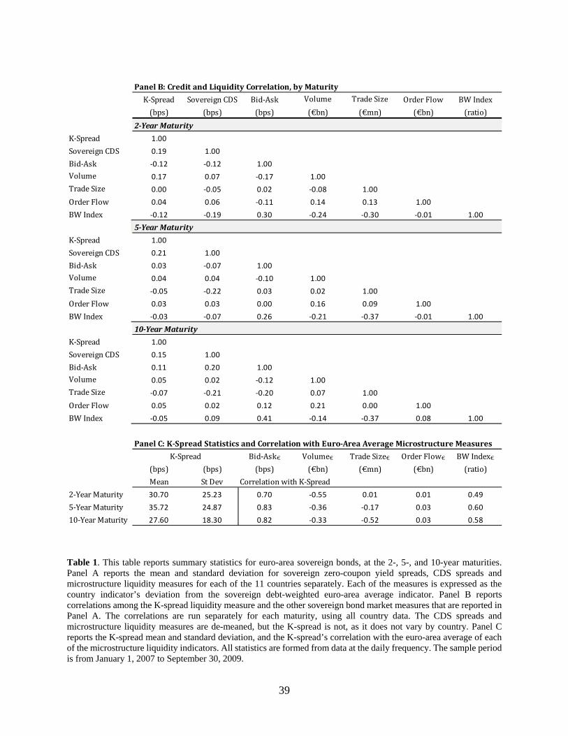
39

 

 

Table 1. This table reports summary statistics for euro-area sovereign bonds, at the 2-, 5-, and 10-year maturities. Panel A reports the mean and standard deviation for sovereign zero-coupon yield spreads, CDS spreads and microstructure liquidity measures for each of the 11 countries separately. Each of the measures is expressed as the country indicator’s deviation from the sovereign debt-weighted euro-area average indicator. Panel B reports correlations among the K-spread liquidity measure and the other sovereign bond market measures that are reported in Panel A. The correlations are run separately for each maturity, using all country data. The CDS spreads and microstructure liquidity measures are de-meaned, but the K-spread is not, as it does not vary by country. Panel C reports the K-spread mean and standard deviation, and the K-spread’s correlation with the euro-area average of each of the microstructure liquidity indicators. All statistics are formed from data at the daily frequency. The sample period is from January 1, 2007 to September 30, 2009.

PanelB:CreditandLiquidityCorrelation,byMaturityK‐Spread SovereignCDS Bid‐Ask Volume TradeSize OrderFlow BWIndex

(bps) (bps) (bps) (€bn) (€mn) (€bn) (ratio)

2‐YearMaturityK‐Spread 1.00SovereignCDS 0.19 1.00Bid‐Ask ‐0.12 ‐0.12 1.00Volume 0.17 0.07 ‐0.17 1.00TradeSize 0.00 ‐0.05 0.02 ‐0.08 1.00OrderFlow 0.04 0.06 ‐0.11 0.14 0.13 1.00BWIndex ‐0.12 ‐0.19 0.30 ‐0.24 ‐0.30 ‐0.01 1.00

5‐YearMaturityK‐Spread 1.00SovereignCDS 0.21 1.00Bid‐Ask 0.03 ‐0.07 1.00Volume 0.04 0.04 ‐0.10 1.00TradeSize ‐0.05 ‐0.22 0.03 0.02 1.00OrderFlow 0.03 0.03 0.00 0.16 0.09 1.00BWIndex ‐0.03 ‐0.07 0.26 ‐0.21 ‐0.37 ‐0.01 1.00

10‐YearMaturityK‐Spread 1.00SovereignCDS 0.15 1.00Bid‐Ask 0.11 0.20 1.00Volume 0.05 0.02 ‐0.12 1.00TradeSize ‐0.07 ‐0.21 ‐0.20 0.07 1.00OrderFlow 0.05 0.02 0.12 0.21 0.00 1.00BWIndex ‐0.05 0.09 0.41 ‐0.14 ‐0.37 0.08 1.00

PanelC:K‐SpreadStatisticsandCorrelationwithEuro‐AreaAverageMicrostructureMeasuresK‐Spread Bid‐Ask€ Volume€ TradeSize€ OrderFlow€ BWIndex€

(bps) (bps) (bps) (€bn) (€mn) (€bn) (ratio)

Mean StDev CorrelationwithK‐Spread

2‐YearMaturity 30.70 25.23 0.70 ‐0.55 0.01 0.01 0.495‐YearMaturity 35.72 24.87 0.83 ‐0.36 ‐0.17 0.03 0.6010‐YearMaturity 27.60 18.30 0.82 ‐0.33 ‐0.52 0.03 0.58

40

Table 2. Interbank Money Market

 

Table 2. This table reports summary statistics for euro-area interbank money markets. Panel A reports the mean and standard deviation of the EURIBOR and OIS rates and spreads at 1-, 3-, 6-, and 12-month maturities. Panel B reports the mean and standard deviation for the one-year maturity K-spread liquidity measure, the overnight bank-tiering credit measure, the overnight interbank market microstructure liquidity measures and the one-year euro-area average bank CDS premia. Correlations among these indicators are also reported. The K-spread is constructed as the one-year KfW yield minus the one-year German federal government yield. The bank-tiering credit measure is formed as the difference in average unsecured interbank borrowing rates paid by the banks in the highest and lowest risk quintiles (estimated in Appendix 1) on each day, using data on overnight interbank borrowing transactions from a large electronic trading platform, e-MID. The market microstructure liquidity measures are also formed with the overnight interbank data. The bank CDS measure is the simple average of the EURIBOR panel banks’ one-year CDS premia on each day. The sample period is from January 1, 2007 to September 30, 2009.

PanelA:InterestRatesandSpreadsbyMaturityEURIBOR OIS EURIBOR‐OIS

(pctpts) (pctpts) (bps)Mean StDev Mean StDev Mean StDev

1‐MonthMaturity 3.33 1.47 3.02 1.45 30.41 29.543‐MonthMaturity 3.63 1.45 3.02 1.48 60.04 42.336‐MonthMaturity 3.73 1.40 3.04 1.51 69.05 48.1912‐MonthMaturity 3.84 1.37 3.09 1.48 75.06 53.88

PanelB:CreditandLiquidityIndicatorsK‐Spread Bank‐Tiering BankCDS Bid‐Ask Volume TradeSize OrderFlow BWIndex

(bps) (bps) (bps) (bps) (€bn) (€mn) (€bn) (ratio)

Mean 26.40 8.27 59.26 4.52 11.29 33.35 ‐7.40 1.01Std.Dev. 23.57 9.03 56.79 6.28 6.15 14.12 4.66 1.91

CorrelationK‐Spread 1.00Bank‐Tiering 0.74 1.00BankCDS 0.69 0.59 1.00Bid‐Ask 0.19 0.39 0.58 1.00Volume ‐0.56 0.22 ‐0.69 ‐0.61 1.00TradeSize ‐0.52 0.37 0.54 0.51 0.15 1.00OrderFlow 0.42 ‐0.48 ‐0.60 ‐0.55 ‐0.58 ‐0.12 1.00BWIndex 0.06 ‐0.44 0.41 0.92 ‐0.90 ‐0.51 0.50 1.00

41

Table 3. Credit versus Liquidity in the Bond Market

      

DependentVariable:SovereignYieldSpreadcmtPanelA:2‐YearMaturityCountry Est. Adj.R2 Est. Adj.R2 Est. Adj.R2 Est. Adj.R2

(SE) (SE) (SE) (SE)

K‐Spread Austria 0.00 0.00 ‐0.10*** 0.47 ‐0.09*** 0.59(0.03) (0.01) (0.01)

Belgium 0.18*** 0.72 0.18*** 0.83 0.18*** 0.86(0.01) (0.00) (0.00)

Finland ‐0.26*** 0.76 ‐0.13*** 0.89 ‐0.15*** 0.92(0.01) (0.00) (0.00)

France ‐0.32*** 0.73 ‐0.15*** 0.96 ‐0.17*** 0.97(0.02) (0.00) (0.00)

Germany ‐0.62*** 0.90 ‐0.40*** 0.98 ‐0.42*** 0.98(0.03) (0.00) (0.00)

Greece 1.60*** 0.72 1.12*** 0.97 1.16*** 0.98(0.13) (0.01) (0.01)

Ireland 1.00*** 0.58 0.28*** 0.75 0.32*** 0.80(0.10) (0.02) (0.02)

Italy 0.59*** 0.83 0.35*** 0.95 0.38*** 0.96(0.02) (0.01) (0.01)

Netherlands ‐0.31*** 0.57 ‐0.28*** 0.78 ‐0.28*** 0.81(0.02) (0.01) (0.01)

Portugal 0.50*** 0.86 0.44*** 0.94 0.44*** 0.94(0.03) (0.00) (0.00)

Spain 0.23*** 0.76 0.15*** 0.83 0.15*** 0.85(0.02) (0.00) (0.00)

SovereignCDSc Joint 0.42*** 0.30 0.31*** 0.27***(0.00) (0.00) (0.00)

Bid‐Askc Joint ‐0.21***(0.05)

Volumec Joint ‐3.96***(0.37)

TradeSizec Joint ‐0.02(0.02)

OrderFlowc Joint 0.27**(0.13)

BWIndexc Joint ‐0.27(0.17)

HypothesisTestsF‐Statistic F‐Statistic F‐Statistic

H0:=0 9244.36*** 2940.57*** 5128.03***H0:=0 4962.43*** 2299.94***H0:=0 16.71***

1cm

2m3m

PanelB:5‐YearMaturityCountry Est. Adj.R2 Est. Adj.R2 Est. Adj.R2 Est. Adj.R2

(SE) (SE) (SE) (SE)

K‐Spread Austria 0.14*** 0.23 ‐0.06*** 0.81 ‐0.06*** 0.82(0.03) (0.00) (0.00)

Belgium 0.29*** 0.84 0.25*** 0.89 0.25*** 0.91(0.01) (0.00) (0.00)

Finland ‐0.08*** 0.23 0.06*** 0.54 0.07*** 0.62(0.01) (0.00) (0.00)

France ‐0.34*** 0.77 ‐0.13*** 0.93 ‐0.13*** 0.94(0.02) (0.00) (0.00)

Germany ‐0.85*** 0.91 ‐0.55*** 0.98 ‐0.55*** 0.99(0.03) (0.00) (0.00)

Greece 2.11*** 0.78 1.32*** 0.94 1.32*** 0.95(0.13) (0.02) (0.02)

Ireland 1.49*** 0.46 0.71*** 0.94 0.69*** 0.94(0.19) (0.02) (0.02)

Italy 0.48*** 0.79 0.26*** 0.93 0.25*** 0.93(0.04) (0.01) (0.01)

Netherlands ‐0.09*** 0.33 ‐0.04*** 0.71 ‐0.03*** 0.74(0.01) (0.00) (0.00)

Portugal 0.56*** 0.79 0.44*** 0.93 0.44*** 0.93(0.03) (0.01) (0.01)

Spain 0.22*** 0.56 0.07*** 0.63 0.07*** 0.64(0.02) (0.00) (0.00)

SovereignCDSc Joint 0.31*** 0.40 0.31*** 0.32***(0.00) (0.00) (0.00)

Bid‐Askc Joint ‐0.03(0.02)

Volumec Joint ‐3.02***(0.49)

TradeSizec Joint ‐0.07***(0.02)

OrderFlowc Joint 0.04(0.13)

BWIndexc Joint ‐0.38***(0.07)

HypothesisTestsF‐Statistic F‐Statistic F‐Statistic

H0:=0 9244.36*** 4969.22*** 4550.69***H0:=0 4345.31*** 4563.43***H0:=0 10.89***

1cm2m3m

1cm

2m3m

42

 

Table 3. This table reports the coefficient estimates from the estimation of equation (3) regressions of yield spreads onto the K-spread liquidity measure alone and on the sovereign CDS spreads alone. The fifth and sixth columns report the results of regressions of yield spreads onto the K-spread and sovereign CDS spreads jointly. The final two columns augment these regressions with sovereign bond market microstructure liquidity measures, as in equation (9). All equations are estimated at the daily frequency over the sample period from January 1, 2007 to September 30, 2009 using seemingly unrelated regressions for each maturity point separately. Newey-West standard errors are in parentheses with the Newey (1994) lag length. One, two and three asterisks denote statistical significance at the 10, 5 and 1, percent levels, respectively. *** indicates significance at the 1 percent level, ** at the 5 percent level, and * at the 10 percent level.

PanelC:10‐YearMaturityCountry Est. Adj.R2 Est. Adj.R2 Est. Adj.R2 Est. Adj.R2

(SE) (SE) (SE) (SE)

K‐Spread Austria 0.15*** 0.19 ‐0.14*** 0.64 ‐0.12*** 0.64(0.04) (0.01) (0.01)

Belgium 0.04 0.02 0.06*** 0.37 0.06*** 0.43(0.03) (0.00) (0.00)

Finland ‐0.35*** 0.76 ‐0.22*** 0.93 ‐0.21*** 0.95(0.02) (0.01) (0.01)

France ‐0.64*** 0.85 ‐0.33*** 0.97 ‐0.34*** 0.97(0.03) (0.00) (0.01)

Germany ‐1.16*** 0.90 ‐0.78*** 0.98 ‐0.77*** 0.98(0.04) (0.01) (0.01)

Greece 2.35*** 0.87 1.52*** 0.94 1.53*** 0.95(0.10) (0.02) (0.02)

Ireland 2.32*** 0.59 1.07*** 0.94 1.09*** 0.94(0.20) (0.02) (0.02)

Italy 0.67*** 0.84 0.51*** 0.97 0.51*** 0.98(0.04) (0.01) (0.01)

Netherlands ‐0.45*** 0.84 ‐0.31*** 0.95 ‐0.32*** 0.96(0.01) (0.00) (0.00)

Portugal 0.43*** 0.59 0.38*** 0.82 0.38*** 0.83(0.06) (0.01) (0.01)

Spain 0.23*** 0.41 0.03*** 0.29 0.05*** 0.42(0.04) (0.01) (0.01)

SovereignCDSc Joint 0.39*** 0.21 0.29*** 0.28***(0.00) (0.00) (0.00)

Bid‐Askc Joint 0.04***(0.01)

Volumec Joint 0.97*(0.50)

TradeSizec Joint ‐0.13***(0.02)

OrderFlowc Joint ‐0.19*(0.10)

BWIndexc Joint 0.19***(0.03)

HypothesisTestsF‐Statistic F‐Statistic F‐Statistic

H0:=0 9244.36*** 3362.65*** 1946.88***H0:=0 1808.37*** 2274.84***H0:=0 39.85***

1cm

2m

3m

1cm

2m3m

43

Table 4. Credit versus Liquidity in the Money Market

DependentVariable:EURIBOR‐OISSpreadm,tRegressionsontoK‐Spreadt,BankTieringCreditMeasuret,BankCDSPremiat,andMicrostructureLiquidityMeasurestPanelA:1‐MonthMaturity PanelB:3‐MonthMaturity

K‐Spread 1.08***   0.94*** 1.23*** 1.29*** 1.67*** 1.61*** 1.78*** 1.76***(0.07) (0.07) (0.05) (0.06) (0.07) (0.08) (0.08) (0.09)

Bank‐Tiering 2.32*** 0.49** 0.74*** 0.58*** 2.31*** 3.30*** 0.20 0.34** 0.14 2.51***(0.20) (0.24) (0.11) (0.12) (0.20) (0.31) (0.22) (0.16) (0.16) (0.27)

BankCDS 0.21*** ‐0.21*** ‐0.25*** ‐0.01 0.42*** ‐0.12*** ‐0.24*** 0.09*(0.04) (0.02) (0.03) (0.04) (0.06) (0.03) (0.03) (0.05)

Bid‐Ask 0.94*** ‐1.46*** 1.39*** ‐1.88***(0.26) (0.51) (0.35) (0.69)

Volume 0.01 ‐1.93** ‐1.22** ‐3.93***(0.33) (0.77) (0.55) (1.07)

TradeSize ‐0.07 ‐0.18 ‐0.14 ‐0.26(0.14) (0.22) (0.14) (0.25)

OrderFlow ‐0.17 ‐1.29*** ‐0.20 ‐1.83***(0.16) (0.41) (0.40) (0.67)

BWIndex ‐1.93** ‐1.17 ‐4.18*** ‐3.07(0.79) (1.49) (1.11) (1.98)

R2‐Adjusted(%) 75.81 50.27 16.08 76.81 85.51 85.87 59.93 86.31 49.53 31.07 86.38 87.76 89.55 66.49

PanelC:6‐MonthMaturity PanelD:12‐MonthMaturityK‐Spread 1.92*** 1.81*** 1.84*** 1.86*** 2.14*** 2.08*** 2.16*** 2.13***

(0.08) (0.09) (0.10) (0.10) (0.09) (0.11) (0.12) (0.12)Bank‐Tiering 3.88*** 0.41** 0.44** 0.20 2.69*** 4.21*** 0.20 0.26 0.06 2.91***

(0.36) (0.20) (0.20) (0.19) (0.30) (0.39) (0.26) (0.25) (0.23) (0.35)BankCDS 0.54*** ‐0.03 ‐0.19*** 0.15*** 0.59*** ‐0.05 ‐0.23*** 0.17**

(0.06) (0.04) (0.04) (0.05) (0.07) (0.05) (0.05) (0.07)Bid‐Ask 1.20*** ‐2.23*** 1.20*** ‐2.74***

(0.31) (0.68) (0.45) (0.86)Volume ‐2.55*** ‐5.40*** ‐3.38*** ‐6.65***

(0.58) (1.03) (0.76) (1.18)TradeSize 0.12 ‐0.01 0.27 0.12

(0.13) (0.22) (0.17) (0.25)OrderFlow ‐0.66* ‐2.37*** ‐1.00** ‐2.96***

(0.39) (0.65) (0.44) (0.72)BWIndex ‐2.67*** ‐1.50 ‐3.31*** ‐1.97

(0.94) (1.81) (1.23) (2.23)R2‐Adjusted(%) 88.39 52.89 40.52 88.64 88.67 91.63 71.92 87.62 49.65 38.03 87.65 87.80 90.49 69.71

44

Table 4. This table reports the results from regressing the EURIBOR-OIS spread at different maturities onto the one-year K-spread liquidity measure, the proposed overnight bank-tiering credit measure, the one-year bank CDS premia, and overnight interbank market microstructure liquidity measures, as in equation (10). The equation is estimated at the daily frequency, over the sample period from January 1, 2007 to September 30, 2009. Newey-West standard errors are in parentheses with the Newey (1994) lag length. *** indicates significance at the 1 percent level, ** at the 5 percent level, and * at the 10 percent level.

   

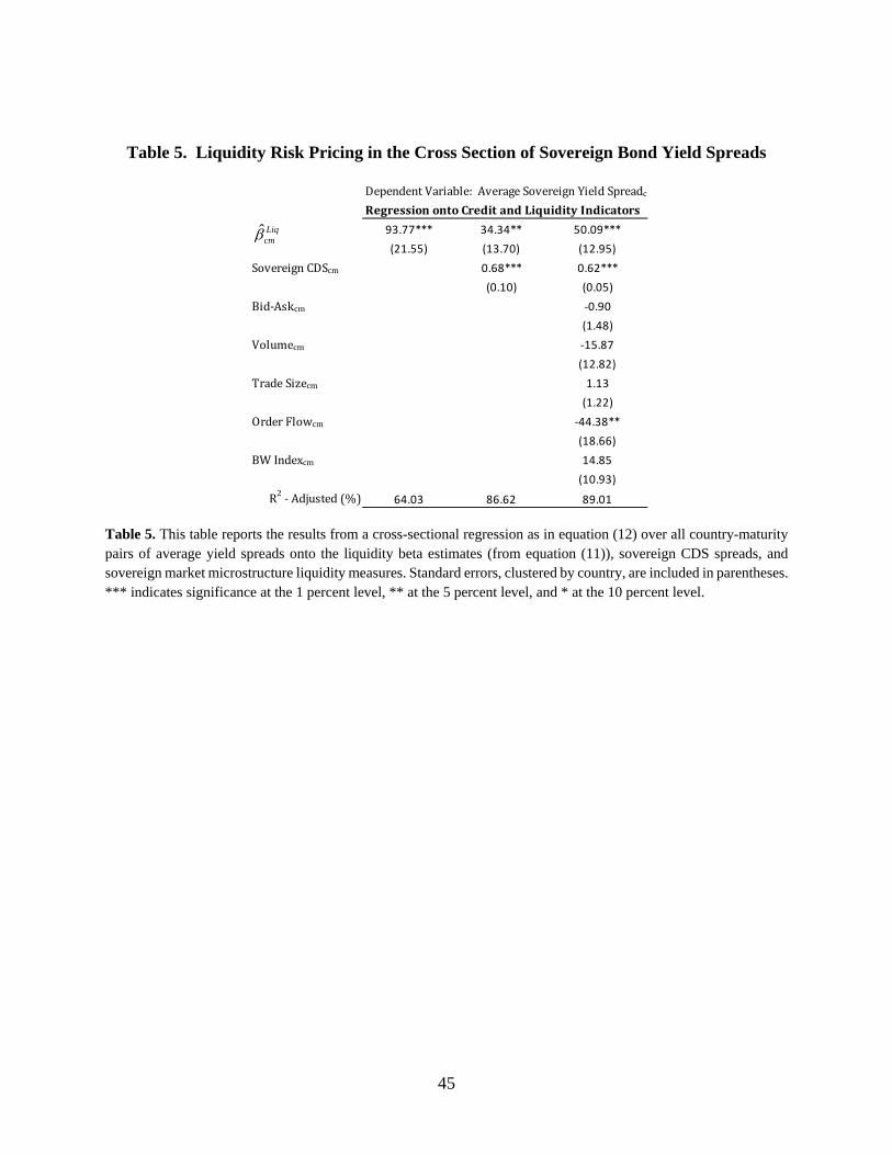
45

 

Table 5. Liquidity Risk Pricing in the Cross Section of Sovereign Bond Yield Spreads

   

Table 5. This table reports the results from a cross-sectional regression as in equation (12) over all country-maturity pairs of average yield spreads onto the liquidity beta estimates (from equation (11)), sovereign CDS spreads, and sovereign market microstructure liquidity measures. Standard errors, clustered by country, are included in parentheses. *** indicates significance at the 1 percent level, ** at the 5 percent level, and * at the 10 percent level.

DependentVariable:AverageSovereignYieldSpreadcmRegressionontoCreditandLiquidityIndicators

93.77*** 34.34** 50.09***(21.55) (13.70) (12.95)

SovereignCDScm 0.68*** 0.62***(0.10) (0.05)

Bid‐Askcm ‐0.90(1.48)

Volumecm ‐15.87(12.82)

TradeSizecm 1.13(1.22)

OrderFlowcm ‐44.38**(18.66)

BWIndexcm 14.85(10.93)

R2‐Adjusted(%) 64.03 86.62 89.01

ˆ Liqcm

46

Figure 1. Euro-Area Government Bond Market  

Panel A:  Country Yields 

5‐Year Maturity 

 

Panel B:  Country Yields minus 11‐Country Average Yield 

5‐Year Maturity 

Figure 1. This figure shows government debt yields (Panel A) and spreads (Panel B) for each of the 11 euro-area countries in the sample, at the 5-year maturity, at a daily frequency. The yield spread is defined as ' '

11' 1cmt cmt c m c mtcy y w y , where

cmty is the sovereign yield spread for country c, at the m-year maturity point,

on day t, minus the euro-area weighted-average yield, as in Equations (2) and (3). The weights are defined as 11

1

,cmcm

c mc

Qw

Q

where cmQ is the quantity of debt

outstanding for each country, c, at each maturity point m and c is a counter variable indexing each of the countries for the purpose of computing the euro-area weighted average. These are based on zero-coupon yields, formed from smoothed curves fitted to all coupon securities, estimated separately for each country and each day.

47

Figure 2. Euro-Area Money Market 

 

Panel A:  EURIBOR Rates 

1‐, 3‐, 6‐, 12‐Month Maturities 

 

   

Panel B:  EURIBOR minus OIS Interest Rate Spreads 

1‐, 3‐, 6‐, 12‐Month Maturities 

  Figure 2. This figure shows interest rate levels (Panel A) and spreads (Panel B) for euro-area interbank money markets for the 1-, 3- , 6- and 12-month maturities, at a daily frequency. Panel A shows the level of EURIBOR rates. Panel B shows the EURIBOR-OIS interest rate spread, defined as the EURIBOR rate minus the comparable-maturity OIS rate.

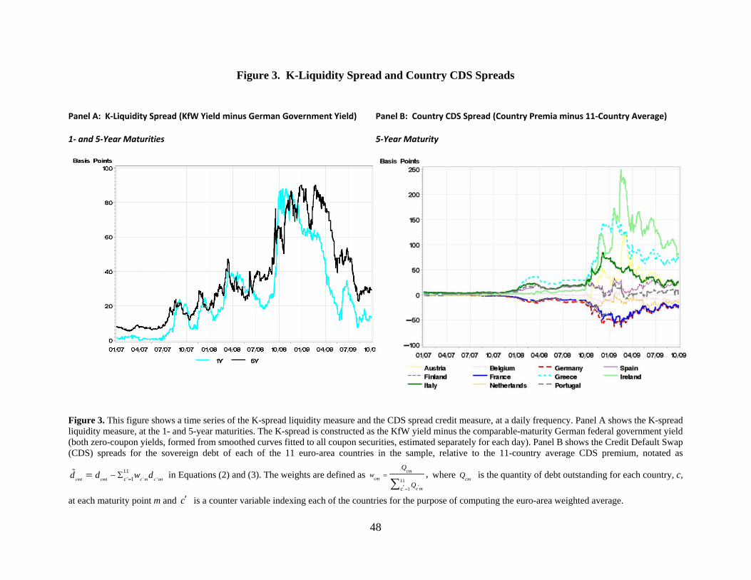
48

Figure 3. K-Liquidity Spread and Country CDS Spreads

 

Panel A:  K‐Liquidity Spread (KfW Yield minus German Government Yield) 

1‐ and 5‐Year Maturities 

 

 

 

Panel B:  Country CDS Spread (Country Premia minus 11‐Country Average) 

5‐Year Maturity 

Figure 3. This figure shows a time series of the K-spread liquidity measure and the CDS spread credit measure, at a daily frequency. Panel A shows the K-spread liquidity measure, at the 1- and 5-year maturities. The K-spread is constructed as the KfW yield minus the comparable-maturity German federal government yield (both zero-coupon yields, formed from smoothed curves fitted to all coupon securities, estimated separately for each day). Panel B shows the Credit Default Swap (CDS) spreads for the sovereign debt of each of the 11 euro-area countries in the sample, relative to the 11-country average CDS premium, notated as

' '

11' 1cmt cmt c m c mtcd d w d in Equations (2) and (3). The weights are defined as

11

1

,cmcm

c mc

Qw

Q

where cmQ is the quantity of debt outstanding for each country, c,

at each maturity point m and c is a counter variable indexing each of the countries for the purpose of computing the euro-area weighted average.

49

Figure 4. Money Market Credit Measures

 

Panel A:  Bank‐Tiering Credit Spread  

1‐Day Maturity 

 

 

Panel B:  Average EURIBOR‐Panel Bank CDS Premia  

1‐Year Maturity 

Figure 4. This figure plots the time series of the two credit measures used to decompose interbank money market spreads at a daily frequency. Panel A shows the overnight bank-tiering credit measure, which is formed as the difference in average unsecured interbank borrowing rates paid by the banks in the highest and lowest risk quintiles (estimated in Appendix 1) on each day. Panel B shows the one-year bank CDS measure, which is the simple average of the EURIBOR panel banks’ one-year CDS premia on each day.

50

Figure 5. Basis Point Change in Sovereign Bond Yield Spreads Explained by One Standard Deviation Shocks to Credit and Liquidity

All Countries (Maturity-Averaged)

 

Figure 5. This figure plots the basis point change in country sovereign bond yield spreads (averaged across maturities) associated with a one standard deviation increase in the country CDS spread (x axis) versus a one standard deviation increase in the K-spread (y axis). The plotted values are based on coefficient estimates from a regression of sovereign bond yield spreads onto the K-spread and the country sovereign CDS spreads, shown in column 5 of Table 3. The country sovereign CDS spread and the K-spread standard deviations are shown in Panels A and C of Table 1.

 

 

51

Figure 6. Basis Point Change in EURIBOR-OIS Spreads Explained by One Standard Deviation Shocks to Credit and Liquidity

  

Figure 6. This figure plots the basis point change in EURIBOR-OIS spreads, by maturity, associated with a one standard deviation increase in the country bank-tiering credit measure (x axis) versus a one standard deviation increase in the K-spread (y axis). The plotted values are based on coefficient estimates from a regression of EURIBOR-OIS spreads onto the K-spread and the bank-tiering credit measure jointly, shown in column 4 in Panels A through D of Table 4. The bank-tiering credit measure and the K-spread standard deviation are shown in Panel B of Table 2.

52

Figure 7. The Sensitivity of Government Bond Yields to Liquidity Risk  

Figure 7. This figure plots the sample-average basis point effect of liquidity risk on sovereign yield spreads, as

estimated in Equation (12), including all controls: 1ˆ Liq

cm . The values are estimated at each maturity point for each

country.