mind the gap - education resources information center · policy information report mind the gap 20...
TRANSCRIPT

POLICY INFORMATION REPORT
MIND THE GAP20 Years of Progress and Retrenchment in School Funding and Achievement Gaps
By Bruce D. Baker, Danielle Farrie and David G. Sciarra
ETS RR-16-15

This Policy Information Report was written by:
Bruce D. BakerRutgers University, New Brunswick, NJ
Danielle Farrie & David G. SciarraEducation Law Center, Newark, NJ
Policy Information CenterMail Stop 19-REducational Testing ServiceRosedale Road Princeton, NJ 08541-0001(609) [email protected]
Copies can be downloaded from:www.ets.org/research/pic
The views expressed in this report are those of the author and do not necessarily reflect the views of the officers andtrustees of Educational Testing Service.
About ETS
At ETS, we advance quality and equity in education for people worldwide by creating assessments based on rigorousresearch. ETS serves individuals, educational institutions and government agencies by providing customized solutionsfor teacher certification, English language learning, and elementary, secondary and postsecondary education, and by con-ducting education research, analysis and policy studies. Founded as a nonprofit in 1947, ETS develops, administers andscores more than 50 million tests annually — including the TOEFL® and TOEIC® tests, the GRE® tests and The PraxisSeries® assessments — in more than 180 countries, at over 9,000 locations worldwide.

Policy Information Report and ETS Research Report Series ISSN 2330-8516
R E S E A R C H R E P O R T
Mind the Gap: 20 Years of Progress and Retrenchment inSchool Funding and Achievement Gaps
Bruce D. Baker,1 Danielle Farrie,2 & David G. Sciarra2
1 Rutgers University, New Brunswick, NJ2 Education Law Center, Newark, NJ
Although there has been significant progress in the long term, achievement gaps among the nation’s students persist. Many factors havecontributed to the disparities in outcomes, and societal changes can explain progress, or lack thereof, over the past few decades. This iswell documented in the 2010 Educational Testing Service (ETS) report Black–White Achievement Gaps: When Progress Stopped, whichexplored achievement gap trends and identified the changing conditions that may have influenced those trends. In this report, we extendthat work by focusing on the relationship between school funding, resource allocation, and achievement among students from low-income families. We tackle the assumption that greater resources, delivered through fair and equitable school funding systems, couldhelp raise academic outcomes and reduce the achievement gap. The goal is to provide convincing evidence that state finance policieshave consequences in terms of the level and distribution of resources, here limited to staffing characteristics, and that the resultingallocation of resources is also associated with changes in both the level of academic achievement and achievement gaps between low-income children and their peers. Using more than 20 years of revenue and expenditure data for schools, we empirically test the ideathat increasing investments in schools generally is associated with greater access to resources as measured by staffing ratios, class sizes,and the competitiveness of teacher wages. When the findings presented here are considered with the strong body of academic literatureon the positive relationship between substantive and sustained state school finance reforms and improved student outcomes, a strongcase can be made that state and federal policy focused on improving state finance systems to ensure equitable funding and improvingaccess to resources for children from low-income families is a key strategy to improve outcomes and close achievement gaps.
Keywords school funding; school finance; funding equity; funding fairness; achievement gap; teacher compensation; class size;school quality; school poverty
doi:10.1002/ets2.12098
In 2010, Educational Testing Service (ETS) released The Black–White Achievement Gap: When Progress Stopped, a reportby Barton and Coley (2010) in which the authors explored the Black–White achievement gap from the 1970s to recentyears. The goal of that report was to explore trends in Black–White achievement gaps and changing conditions that mayexplain those trends. Barton and Coley explained that “from the early 1970s until the late 1980s, a very large narrowing ofthe gap occurred in both reading and mathematics, with the size of the reduction depending on the subject and age groupexamined” (p. 7). Reductions to achievement gaps were particularly large in reading among 13- and 17-year-olds, whilestill significant in mathematics. However, “during the 1990s, the gap narrowing generally halted, and actually began toincrease in some cases” (p. 7). The authors noted some additional gap narrowing from 1999 to 2004 and mixed findingsfrom 2004 to 2008. Rothstein (2011) showed that, even during the period from 1990 to 2008, achievement gains forBlack fourth- and eighth-grade students have been substantial in mathematics in particular and that these students haveoutpaced their White peers.1
Barton and Coley (2010) offered some broad hypotheses as to policy and contextual changes that may partly explainthe faster rate of gap reduction that occurred during the earlier periods. For example, the authors noted that the pastseveral decades have been a time of increased investment in early education programs made available to low-income andminority children; reduction in racially disparate tracking in America’s middle and high schools; class size and pupil-to-teacher ratio reduction; desegregation; and increased emphasis on testing and accountability, including a focus on racialachievement gaps.
Other recent reports have focused more broadly on trends in income and racial inequality among children in theUnited States over recent decades (Coley & Baker, 2013; Reardon, 2011). Specifically, there has been increased emphasis
Corresponding author: B. D. Baker, E-mail: [email protected]
Policy Information Report and ETS Research Report Series No. RR-16-15. © 2016 Educational Testing Service 1

B. D. Baker et al. 20 Years of Progress in School Funding
on income inequality built on assertions that income-based achievement gaps now far surpass racially based achievementgaps. For example, Reardon noted that “the achievement gap between children from high- and low-income families isroughly 30 to 40 percent larger among children born in 2001 than among those born twenty-five years earlier” (p. 1).Furthermore,
the income achievement gap (defined here as the average achievement difference between a child from a family at the90th percentile of the family income distribution and a child from a family at the 10th percentile) is now nearly twiceas large as the Black–White achievement gap. (p. 1)
This report builds on the earlier work of Barton and Coley (2010) by longitudinally tracking achievement gaps andpotential factors explaining both the ebbs and flows of those gaps and cross-state variation in those gaps over time. But, likeReardon (2011) and Coley and Baker (2013), we focus on income inequality—specifically child poverty—in evaluatinggaps in both available educational resources and measured educational outcomes. We focus on the distribution of childrenliving in poverty and below various low-income thresholds across U.S. public schools, differences in resources availableto those children, and differences in measured outcomes of children falling under various income thresholds. AppendixA provides a brief explanation of the relationship between income-based and racially based achievement gaps.
We begin with a review of the literature on how and why money matters, focusing on equitable and adequate funding,class sizes and teacher salaries, and the role of state school finance systems in ensuring equal educational opportunity. Thisis followed by an examination of trends in school revenues, staffing, and wages over time to demonstrate the relationshipbetween increased funding and the availability of resources, particularly for children from low-income families. Under-standing that school funding and resource distribution vary widely by state as a function of the dominance of state andlocal financing of U.S. public schools; we focus our analyses at the state level. The time period of the analysis also allowsfor some speculation on the consequences of the Great Recession for school funding fairness and resource equity. Finally,we show that the level and distribution of resources relative to poverty are associated with higher academic outcomes forchildren from low-income families and a narrowing of achievement gaps by income.
How and Why Money Matters in Schools
Expanding on Barton and Coley’s (2010) exploration of potential factors explaining achievement gap reduction, we focusherein on measures of funding and key resources available to children’s schools and how those resources have been dis-tributed with respect to low-income populations over time. Our emphasis on funding and related resources warrants somejustification. In a comprehensive review of literature addressing the question “Does money matter in education?” Baker(2012) concluded,
To be blunt, money does matter. Schools and districts with more money clearly have greater ability to providehigher-quality, broader, and deeper educational opportunities to the children they serve. Furthermore, in theabsence of money, or in the aftermath of deep cuts to existing funding, schools are unable to do many of the thingsthey need to do in order to maintain quality educational opportunities. Without funding, efficiency tradeoffs andinnovations being broadly endorsed are suspect. One cannot tradeoff spending money on class size reductionsagainst increasing teacher salaries to improve teacher quality if funding is not there for either—if class sizes arealready large and teacher salaries non-competitive. While these are not the conditions faced by all districts, they arefaced by many. (p. 18)
Building on the findings and justifications Baker (2012) provided, we offer Figure 1 as a simple model of the relationshipof schooling resources to children’s measurable school achievement outcomes. First, the fiscal capacity of states—theirwealth and income—does affect their ability to finance public education systems. But, as we have shown in relatedresearch, on which we expand herein, the effort put forth in state and local tax policy plays an equal role (Baker, Farrie, &Sciarra, 2010).
The amount of state and local revenue raised drives the majority of current spending of local public school districts,because federal aid constitutes such a relatively small share. Furthermore, the amount of money a district is able spend oncurrent operations determines the staffing ratios, class sizes, and wages a local public school district is able to pay. Indeed,
2 Policy Information Report and ETS Research Report Series No. RR-16-15. © 2016 Educational Testing Service

B. D. Baker et al. 20 Years of Progress in School Funding
State & Local Fiscal Effort
State & Local Wealth & Income
State & Local
Revenue
Current Operating
Expenditure
Staffing Quantities (Pupil to Teacher Ratio
& Class Size)
Staffing Quality (Competitive
Wage)
Student Outcomes
Figure 1 Conceptual map of the relationship of schooling resources to children’s measurable school achievement outcomes.
there are trade-offs to be made between staffing ratios and wage levels. Finally, a sizable body of research has illustratedthe connection between staffing qualities and quantities and student outcomes (see Baker, 2012).
The connections laid out in this model appear rather obvious. How much you raise dictates how much you can spend.How much you spend in a labor-intensive industry dictates how many individuals you can employ, the wage you can paythem, and in turn the quality of individuals you can recruit and retain. But in this modern era of resource-free schoolreforms, the connections between revenue, spending, and real, tangible resources are often ignored or, worse, argued tobe irrelevant. A common theme advanced in modern political discourse is that all schools and districts already have morethan enough money to get the job done. They simply need to use it more wisely and adjust to the new normal (Baker &Welner, 2012).
But, on closer inspection of the levels of funding available across states and local public school districts within states,this argument rings hollow. To illustrate, a significant portion of this report statistically documents these connections.First, we take a quick look at existing literature on the relevance of state school finance systems and on the reform of thosesystems for improving the level and distribution of student outcomes as well as literature on the importance of class sizesand teacher wages for improving school quality as measured by student outcomes.
Equitable and Adequate Funding
An increasing body of evidence suggests that substantive and sustained state school finance reforms matter for improvingboth the level and distribution of short-term and long-run student outcomes. A few studies have attempted to tackleschool finance reforms broadly by applying multistate analyses over time. Card and Payne (2002) found “evidence thatequalization of spending levels leads to a narrowing of test score outcomes across family background groups” (p. 49).Most recently, Jackson, Johnson, and Persico (2015) evaluated long-term outcomes of children exposed to court-orderedschool finance reforms, finding that
a 10 percent increase in per-pupil spending each year for all twelve years of public school leads to 0.27 morecompleted years of education, 7.25 percent higher wages, and a 3.67 percentage-point reduction in the annualincidence of adult poverty; effects are much more pronounced for children from low-income families. (p. 1)
Numerous other researchers have explored the effects of specific state school finance reforms over time.2 Several suchstudies have provided compelling evidence of the potential positive effects of school finance reforms. Studies of Michiganschool finance reforms in the 1990s have shown positive effects on student performance in both the previously lowestspending districts (Roy, 2011)3 and previously lower performing districts (Papke, 2005). Similarly, a study of Kansas schoolfinance reforms in the 1990s, which also involved primarily a leveling up of low-spending districts, found that a 20%increase in spending was associated with a 5% increase in the likelihood of students going on to postsecondary education(Deke, 2003).
Three studies of Massachusetts school finance reforms from the 1990s found similar results. The first, by Downes,Zabel, and Ansel (2009), found that the combination of funding and accountability reforms “has been successful in raising
Policy Information Report and ETS Research Report Series No. RR-16-15. © 2016 Educational Testing Service 3

B. D. Baker et al. 20 Years of Progress in School Funding
the achievement of students in the previously low-spending districts” (p. 5). The second found that increases in per pupilspending led to significant increases in mathematics, reading, science, and social studies test scores for fourth- and eighth-grade students (Guryan, 2001).4 The most recent of the three found that “changes in the state education aid following theeducation reform resulted in significantly higher student performance” (Nguyen-Hoang & Yinger, 2014, p. 297). Suchfindings have been replicated in other states, including Vermont.5
On balance, it is safe to say that a sizable and growing body of rigorous empirical literature has validated that state schoolfinance reforms can have substantive, positive effects on student outcomes, including reductions in outcome disparitiesor increases in overall outcome levels.6
Class Sizes and Teacher Salaries
The premise that money matters for improving school quality is grounded in the assumption that having more moneyprovides schools and districts the opportunity to improve the qualities and quantities of real resources. Jackson et al.(2015) explained that the spending increases they found to be associated with long-term benefits “were associated withsizable improvements in measured school quality, including reductions in student-to-teacher ratios, increases in teachersalaries, and longer school years” (p. 1).
The primary resources involved in the production of schooling outcomes are human resources—or quantities andqualities of teachers, administrators, support, and other staff in schools. Quantities of school staff are reflected in pupil-to-teacher ratios and average class sizes. Reduction of class sizes or reductions of overall pupil-to-staff ratios requireadditional staff, thus additional money, assuming the wages and benefits for additional staff remain constant. Qualities ofschool staff depend in part on the compensation available to recruit and retain the staff—specifically salaries and benefits,in addition to working conditions. Notably, working conditions may be reflected in part through measures of workload,such as average class sizes, as well as the composition of the student population.
A substantial body of literature has accumulated to validate the conclusion that teachers’ overall wages and relativewages affect the quality of those who choose to enter the teaching profession—and whether they stay once they get in.For example, Murnane and Olsen (1989) found that salaries affect the decision to enter teaching and the duration of theteaching career, whereas Figlio (1997, 2002) and Ferguson (1991) concluded that higher salaries are associated with morequalified teachers. In addition, more recent studies have tackled the specific issues of relative pay noted earlier. Loeb andPage (2000) showed that
once we adjust for labor market factors, we estimate that raising teacher wages by 10 percent reduces high schooldropout rates by 3 percent to 4 percent. Our findings suggest that previous studies have failed to produce robustestimates because they lack adequate controls for non-wage aspects of teaching and market differences in alternativeoccupational opportunities. (p. 393)
In short, although salaries are not the only factor involved, they do affect the quality of the teaching workforce, whichin turn affects student outcomes. A permanent upward shift in the competitiveness of teacher wages may substantivelyimprove the quality of the teacher workforce and, ultimately, student outcomes.
Research on the flip side of this issue—evaluating spending constraints or reductions—has revealed the potentialharm to teaching quality that flows from leveling down or reducing spending. For example, Figlio and Rueben (2001)noted that “using data from the National Center for Education Statistics we find that tax limits systematically reduce theaverage quality of education majors, as well as new public school teachers in states that have passed these limits” (p. 1; seealso Downes & Figlio, 1999).
Salaries also play a potentially important role in improving the equity of student outcomes. Although several studieshave shown that higher salaries relative to labor market norms can draw higher quality candidates into teaching, theevidence also indicates that relative teacher salaries across schools and districts may influence the distribution of teachingquality. For example, Ondrich, Pas, and Yinger (2008) found
that teachers in districts with higher salaries relative to non-teaching salaries in the same county are less likely toleave teaching and that a teacher is less likely to change districts when he or she teaches in a district near the top ofthe teacher salary distribution in that county. (p. 112)
4 Policy Information Report and ETS Research Report Series No. RR-16-15. © 2016 Educational Testing Service
B. D. Baker et al. 20 Years of Progress in School Funding
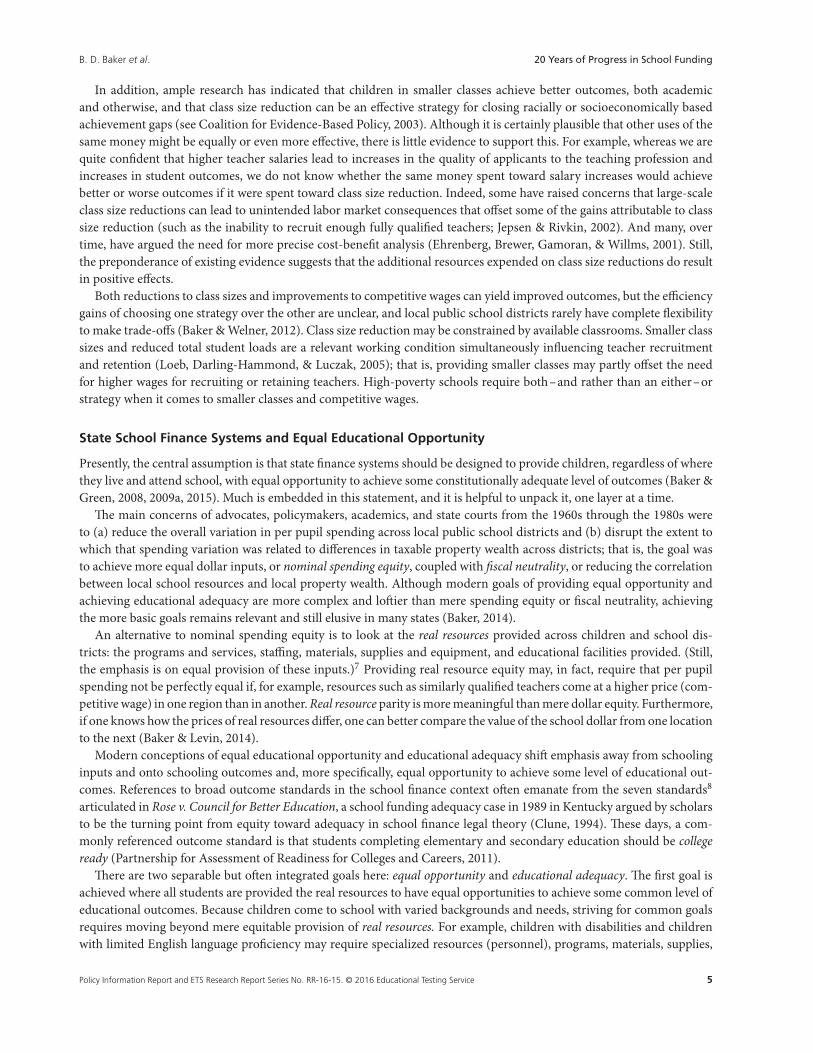
In addition, ample research has indicated that children in smaller classes achieve better outcomes, both academicand otherwise, and that class size reduction can be an effective strategy for closing racially or socioeconomically basedachievement gaps (see Coalition for Evidence-Based Policy, 2003). Although it is certainly plausible that other uses of thesame money might be equally or even more effective, there is little evidence to support this. For example, whereas we arequite confident that higher teacher salaries lead to increases in the quality of applicants to the teaching profession andincreases in student outcomes, we do not know whether the same money spent toward salary increases would achievebetter or worse outcomes if it were spent toward class size reduction. Indeed, some have raised concerns that large-scaleclass size reductions can lead to unintended labor market consequences that offset some of the gains attributable to classsize reduction (such as the inability to recruit enough fully qualified teachers; Jepsen & Rivkin, 2002). And many, overtime, have argued the need for more precise cost-benefit analysis (Ehrenberg, Brewer, Gamoran, & Willms, 2001). Still,the preponderance of existing evidence suggests that the additional resources expended on class size reductions do resultin positive effects.
Both reductions to class sizes and improvements to competitive wages can yield improved outcomes, but the efficiencygains of choosing one strategy over the other are unclear, and local public school districts rarely have complete flexibilityto make trade-offs (Baker & Welner, 2012). Class size reduction may be constrained by available classrooms. Smaller classsizes and reduced total student loads are a relevant working condition simultaneously influencing teacher recruitmentand retention (Loeb, Darling-Hammond, & Luczak, 2005); that is, providing smaller classes may partly offset the needfor higher wages for recruiting or retaining teachers. High-poverty schools require both–and rather than an either–orstrategy when it comes to smaller classes and competitive wages.
State School Finance Systems and Equal Educational Opportunity
Presently, the central assumption is that state finance systems should be designed to provide children, regardless of wherethey live and attend school, with equal opportunity to achieve some constitutionally adequate level of outcomes (Baker &Green, 2008, 2009a, 2015). Much is embedded in this statement, and it is helpful to unpack it, one layer at a time.
The main concerns of advocates, policymakers, academics, and state courts from the 1960s through the 1980s wereto (a) reduce the overall variation in per pupil spending across local public school districts and (b) disrupt the extent towhich that spending variation was related to differences in taxable property wealth across districts; that is, the goal wasto achieve more equal dollar inputs, or nominal spending equity, coupled with fiscal neutrality, or reducing the correlationbetween local school resources and local property wealth. Although modern goals of providing equal opportunity andachieving educational adequacy are more complex and loftier than mere spending equity or fiscal neutrality, achievingthe more basic goals remains relevant and still elusive in many states (Baker, 2014).
An alternative to nominal spending equity is to look at the real resources provided across children and school dis-tricts: the programs and services, staffing, materials, supplies and equipment, and educational facilities provided. (Still,the emphasis is on equal provision of these inputs.)7 Providing real resource equity may, in fact, require that per pupilspending not be perfectly equal if, for example, resources such as similarly qualified teachers come at a higher price (com-petitive wage) in one region than in another. Real resource parity is more meaningful than mere dollar equity. Furthermore,if one knows how the prices of real resources differ, one can better compare the value of the school dollar from one locationto the next (Baker & Levin, 2014).
Modern conceptions of equal educational opportunity and educational adequacy shift emphasis away from schoolinginputs and onto schooling outcomes and, more specifically, equal opportunity to achieve some level of educational out-comes. References to broad outcome standards in the school finance context often emanate from the seven standards8
articulated in Rose v. Council for Better Education, a school funding adequacy case in 1989 in Kentucky argued by scholarsto be the turning point from equity toward adequacy in school finance legal theory (Clune, 1994). These days, a com-monly referenced outcome standard is that students completing elementary and secondary education should be collegeready (Partnership for Assessment of Readiness for Colleges and Careers, 2011).
There are two separable but often integrated goals here: equal opportunity and educational adequacy. The first goal isachieved where all students are provided the real resources to have equal opportunities to achieve some common level ofeducational outcomes. Because children come to school with varied backgrounds and needs, striving for common goalsrequires moving beyond mere equitable provision of real resources. For example, children with disabilities and childrenwith limited English language proficiency may require specialized resources (personnel), programs, materials, supplies,
Policy Information Report and ETS Research Report Series No. RR-16-15. © 2016 Educational Testing Service 5

B. D. Baker et al. 20 Years of Progress in School Funding
and equipment. Schools and districts serving larger shares of these children may require substantively more fundingto provide these resources. Furthermore, where poverty is highly concentrated, smaller class sizes and other resource-intensive interventions may be required to strive for those outcomes commonly achieved by the state’s average child.
Meanwhile, conceptions of educational adequacy require that policymakers determine the desired level of outcometo be achieved. It may well be that the outcomes achieved by the average child are deemed to be sufficient. But it mayalso be the case that the preferences of policymakers or a specific legal mandate are somewhat higher (or lower) than theoutcomes achieved by the average child. Essentially, adequacy conceptions attach a “level” of outcome expectation to theequal educational opportunity concept.
Modern state school finance formulas—aid distribution formulas—strive to achieve two simultaneous objectives:(a) accounting for differences in the costs of achieving equal educational opportunity across schools and districts and(b) accounting for differences in the ability of local public school districts to cover those costs. Local district ability toraise revenues might be a function of either or both local taxable property wealth and the incomes of local propertyowners, thus their ability to pay taxes on their properties.
In a typical state school finance formula, it is implied that some basic funding level should be sufficient for producing agiven level of student outcomes in an average school district. It is then assumed that if one wishes to produce a higher levelof outcomes, the foundation level should be increased. In short, it costs more to achieve higher outcomes (Duncombe &Yinger, 1999), and the foundation level in a state school finance formula is the tool used for determining the overall levelof support to be provided.
Furthermore, it is assumed that resource levels may be adjusted to permit districts in different parts of a state to recruitand retain teachers of comparable quality; that is, the wages paid to teachers affect who will be willing to work in any givenschool. In other words, teacher wages affect teacher quality, and in turn, they affect school quality and student outcomes.This is plain common sense, and this teacher wage effect operates at two levels. First, in general, teacher wages must besufficiently competitive with other career opportunities for similarly educated individuals. The overall competitiveness ofteacher wages affects the overall academic quality of those who choose to enter teaching (Allegretto, Corcoran, & Mishel,2008; Ferguson, 1991; Figlio, 1997, 2002; Figlio & Rueben, 2001; Loeb & Page, 2000; Murnane & Olsen, 1989). Second, therelative wages for teachers across local public school districts determine the distribution of teaching quality (Clotfelter,Glennie, Ladd, & Vigdor, 2008; Clotfelter, Ladd, & Vigdor, 2011; Lankford, Loeb, & Wyckoff, 2002; Ondrich et al., 2008).Districts with more favorable working conditions (more desirable facilities, fewer students from low-income families andminority students) can pay a lower wage and attract the same teacher.
Finally, student need adjustments in state school finance formulas assume that the additional resources can be leveragedto improve outcomes for students from low-income families or students with limited English language proficiency. First,note that some share of the additional resources is needed in higher poverty settings simply to provide for “real resource”equity—or to pay the wage premium for doing the more complicated job, under less desirable working conditions. Sec-ond, resource-intensive strategies such as reduced class sizes in the early grades, high-quality (using qualified teachingstaff; Barnett, 2003) early childhood programs, intensive tutoring, and extended learning time programs may significantlyimprove outcomes of students from low-income families. And these strategies all come with significant additional costs.
As such, as a rule of thumb, for a state school finance system to provide equal educational opportunity, that system mustensure sufficiently higher resources in higher need (higher poverty) settings than in lower need settings. We characterizesuch a system herein as progressive. By contrast, many state school finance systems barely achieve “flat” funding betweenhigh- and low-need settings, and still others remain regressive.
Tracking Indicators of Funding, Key Resources, and Outcomes
In this section, we explore 20 years of changes in school funding across states in relation to specific educational resourcesand student outcomes. Table 1 summarizes the indicators we explore herein, each intended to illustrate the linkages in ourconceptual map from state financing to student outcomes. We begin with financial indicators, establishing the connectionbetween state and local revenues per pupil and current operating spending per pupil. Data sources are elaborated inAppendix B.
In each case where we measure revenues or expenditures, our data are annual from 1993 to 2012 and are at the levelof the local public school district. Our intent is, to the extent possible, to create an equated dollar value across settings.We use statistical models fit to our district-level data to predict the level of funding available in a K–12 district enrolling
6 Policy Information Report and ETS Research Report Series No. RR-16-15. © 2016 Educational Testing Service

B. D. Baker et al. 20 Years of Progress in School Funding
Table 1 Indicators
Indicator type Levels and adequacy Distribution and equity
Financial inputs Fiscal Indicator 1: Local revenue perpupil for a K–12 district with 10%Census poverty, 2,000 or morestudents, in an average wage labormarket.
Fiscal Indicator 2: State aid per pupil fora K–12 district with 10% Censuspoverty, 2,000 or more students, in anaverage wage labor market.
Fiscal Indicator 3: Federal aid per pupilfor a K–12 district with 10% Censuspoverty, 2,000 or more students, in anaverage wage labor market.
Fiscal Indicator 4: Current spending perpupil for a K–12 district with 10%Census poverty, 2,000 or morestudents, in an average wage labormarket.
Input Equity Indicator 1: Current spending fairness ratio.Predicted current spending per pupil for a district with 30%poverty divided by predicted current spending per pupil fora district with 0% poverty, for K–12 districts with 2,000 ormore students, in an average wage labor market.
• Current spending fairness ratio of 1.2 indicates that ahigh-poverty district is expected to have 20% higher perpupil spending than a low-poverty district, and the system isprogressive.
• Current spending fairness ratio of 0.80 indicates that ahigh-poverty district is expected to have only 80% of thespending of a low-poverty district, and the system isregressive.
Input Equity Indicator 2: State and local revenue fairness ratio.Predicted state and local revenue per pupil for a district with30% poverty divided by predicted state and local revenue perpupil for a district with 0% poverty, for K–12 districts with2,000 or more students, in an average wage labor market.
• State and local revenue fairness ratio of 1.2 indicates that ahigh-poverty district is expected to have 20% higher perpupil revenue than a low-poverty district, and the system isprogressive.
• State and local revenue fairness ratio of 0.80 indicates that ahigh-poverty district is expected to have only 80% of therevenue of a low-poverty district, and the system isregressive.
Real resources Resource Input 1: Teachers per 100 pupilsfor a K–12 district with 10% Censuspoverty, 2,000 or more students, in anaverage wage labor market.
Resource Input 2: Competitive wageratio. Predicted wage of elementaryand secondary teachers divided bypredicted wage of nonteachersworking in the same state, withmaster’s degree, at specific ages.
Input Equity Indicator 3: Teachers per 100 pupils fairness ratio.Predicted teachers per 100 pupils for a district with 30%poverty divided by predicted teachers per 100 pupils for adistrict with 0% poverty, for K–12 districts with 2,000 ormore students, in an average wage labor market.
• Teachers per 100 pupils fairness ratio of 0.80 indicates that ahigh-poverty district is expected to have 80% of the teachersper 100 pupils of a low-poverty district, and the system isregressive.
• Teachers per 100 pupils fairness ratio of 1.2 indicates that ahigh-poverty district is expected to have 20% higher teachersper 100 pupils than a low-poverty district, and the system isprogressive.
Outcomes Outcome Level Indicator 1: Low-incomestudents’ performance level.Standardized difference betweenactual and expected NAEP scalescore for students from low-incomefamilies (given mean income oflow-income families).
Outcome Gap Indicator 1: Low-income achievement gap.Standardized difference in NAEP mean scale scores ofchildren from low-income families (children with free lunch)versus children from non-low-income families, corrected fordifferences in the mean income levels of the two groups.
Outcome Gap Indicator 2: Income achievement effect. Statisticalrelationship across schools within states between school-levelconcentration of children from low-income families andschool-level expected NAEP mean scale score.
Note. NAEP=National Assessment of Educational Progress.
Policy Information Report and ETS Research Report Series No. RR-16-15. © 2016 Educational Testing Service 7
B. D. Baker et al. 20 Years of Progress in School Funding
at least 2,000 pupils, in an average competitive wage (national mean) labor market and at varied levels of child povertyconcentration. Our goals are twofold: (a) to have comparable predicted resource measures across states at fixed povertyrates and (b) to have indicators of the extent to which funding varies across districts by poverty concentration withinstates. Statistical models are presented in Appendix C. All of our fiscal input indicators apply the same approach.
Next we move to real resource indicators. The first real resource indicator we explore is a staffing quantity measure:numbers of teaching staff per 100 pupils. We opt for this measure in place of the more common pupil-to-teacher ratio (itsinverse) because this measure moves in the same direction as our other measures—wherein higher levels on the measureindicate more resources per pupil. Our staffing quantity indicators are constructed by the same method as our financialindicators: Using annual district-level data, we predict teachers per 100 pupils across states at a fixed district poverty rateand within states at varied district poverty rates.
We also explore the relative competitiveness of teacher wages across states using U.S. Census data on individuals holdinga bachelor’s or master’s degree and between the ages of 25 and 45 years. We use these data to estimate the relative annualwage of elementary and secondary teachers to nonteachers, at constant age and degree level. This indicator serves asa measure of the relative adequacy of teacher wages across states. We can expect, for example, that in states in whichteacher wages are more comparable to other employment options, individuals may be more likely to choose teaching asa career. But, because we do not know the school districts in which these individuals teach, we are unable to evaluate thedistribution of teacher wages with respect to school district child poverty concentration.
Finally, for our outcome measures, we rely on the National Assessment of Educational Progress (NAEP). For stateperformance levels, we focus specifically on the mean performance of children from low-income families. But, becausethe mean performance of children from low-income families varies with respect to the income levels of children fromlow-income families across states, we re-express NAEP average performance to account for these differences. That is, theincome level of low-income families varies by state. In states where that income level is higher, NAEP tends to be higher,and vice versa. We condition the average performance on the average income levels of students from low-income familiesin the state and express performance levels as standardized differences between the expected performance level (givenincome levels) and actual performance levels (see Appendix C for more information on variable construction).
We make similar adjustments to our achievement gap measures; that is, we start with a simple measure of the achieve-ment gap—mean performance difference—between children from families who do not qualify for free lunch and childrenfrom families who do qualify for free lunch. But the income gap between these groups varies by state. Furthermore,states with bigger income gaps between low-income and non-low-income families tend to have bigger performance gapsbetween these same groups (correlations in Appendix D). Our approach is to condition our achievement gap measures onthe income gap and express achievement gaps as standardized differences between the expected achievement gap (givenincome gap) and actual achievement gap.9
Public School Revenues Over Time
We begin by exploring local public school district revenues over time, tracking the following indicators:
Fiscal Indicator 1: Local revenue per pupil for a K–12 district with 10% Census poverty and 2,000 or more students, inan average wage labor market.Fiscal Indicator 2: State aid per pupil for a K–12 district with 10% Census poverty and 2,000 or more students, in anaverage wage labor market.Fiscal Indicator 3: Federal aid per pupil for a K–12 district with 10% Census poverty and 2,000 or more students, in anaverage wage labor market.Fiscal Indicator 4: Current spending per pupil for a K–12 district with 10% Census poverty and 2,000 or morestudents, in an average wage labor market.
Figure 2 presents the national averages of current spending per pupil and state and local revenues per pupil, adjusted forchanges in labor costs by dividing each district’s revenue or spending figure by the comparable wage index for that district.Both revenues and spending are included to illustrate how the two largely move together over time, as one would expect.The Education Comparable Wage Index adjusts for both regional variation in labor costs (input prices) and inflationarychange in labor costs. Figure 2 shows that, on average, using district-level data weighted by student enrollments, state and
8 Policy Information Report and ETS Research Report Series No. RR-16-15. © 2016 Educational Testing Service

B. D. Baker et al. 20 Years of Progress in School Funding
$0
$1,000
$2,000
$3,000
$4,000
$5,000
$6,000
$7,000
$8,000
$9,000
19
92
19
94
19
96
19
98
20
00
20
02
20
04
20
06
20
08
20
10
20
12
Ad
just
ed p
er P
up
il ($
1999
)
Year
Current Spending (adj.) State & Local Revenue (Adj.)
Figure 2 Input price-adjusted revenue and spending. Data are from current spending per pupil and state and local revenue per pupilfrom the U.S. Census Fiscal Survey of Local Governments (U.S. Census Bureau, n.d.-a), adjusted by dividing by Education ComparableWage Index (Taylor, 2014).
local revenues, and per pupil spending is up approximately 4.5–5.5% over the period, reaching a high in approximately2008 and returning to levels comparable to 2000 by 2012.
Figure 3 tracks the local, state, and federal revenues per pupil (predicted from our model for a district of constantcharacteristics) for each state from 1993 to 2012. In most cases, federal revenue remains relatively trivial, revealing onlya small temporary bump when federal stimulus funds flowed in 2010–2011. State and local revenues tend to play coun-terbalancing roles, most noticeable in states such as New Jersey, New York, and Texas. When state aid is increased,pressure is taken off local revenue sources, but when state aid is cut, local revenues are increased by many districts tooffset their losses. However, with increased dependence on local revenue often comes increased inequity based on vari-ations in local wealth. In many states in Figure 3, state aid cuts in the recent recession were substantial and have notrebounded.
In some states, abrupt policy changes, such as reclassification, recapture, and distribution of property tax revenues,lead to abrupt switches in state and local roles. In Vermont and New Hampshire, a share of property tax revenues wasreclassified as state revenues and redistributed. In Michigan, state sales and sin taxes were dramatically increased in the1990s to substitute for property taxes.
Tracking School Staffing Over Time
Next we track predicted teachers per 100 pupils over time by state:
Resource Input 1: Teachers per 100 pupils for a K–12 district with 10% Census poverty and 2,000 or more students, inan average wage labor market.
It is broadly acknowledged that over the past several decades, nationally, pupil-to-teacher ratios have declined, andthus numbers of teachers per 100 pupils have climbed (Kena et al., 2015). But there has been little attention to morerecent trends or how those trends vary by state. Figure 4 presents national trends for all local public school districts, andthen for K–12 unified school districts and sufficiently large (>2,000 students) K–12 unified districts. Indeed, numbers ofteachers per 100 pupils are higher than they were in the early 1990s. But since 2008, there has been a significant downturnin staffing, which, by 2012, was on average lower than 12 years earlier (in 2000).
Of course, overall levels and trends in staffing per pupil vary by state. State-level patterns do include some unexplainedvolatility in specific years, but overall patterns are consistent with national averages, wherein staffing per pupil generallyincreased since the early 1990s and has declined in recent years. Some states, such as New Jersey, already had relativelyhigh staffing per pupil, whereas others, such as Pennsylvania, did not. Despite national trends, many states, including Wis-consin, Idaho, Oregon, Washington, Colorado, Montana, Utah, and Oklahoma, never experienced substantive increasesin staffing ratios.
Policy Information Report and ETS Research Report Series No. RR-16-15. © 2016 Educational Testing Service 9

B. D. Baker et al. 20 Years of Progress in School Funding
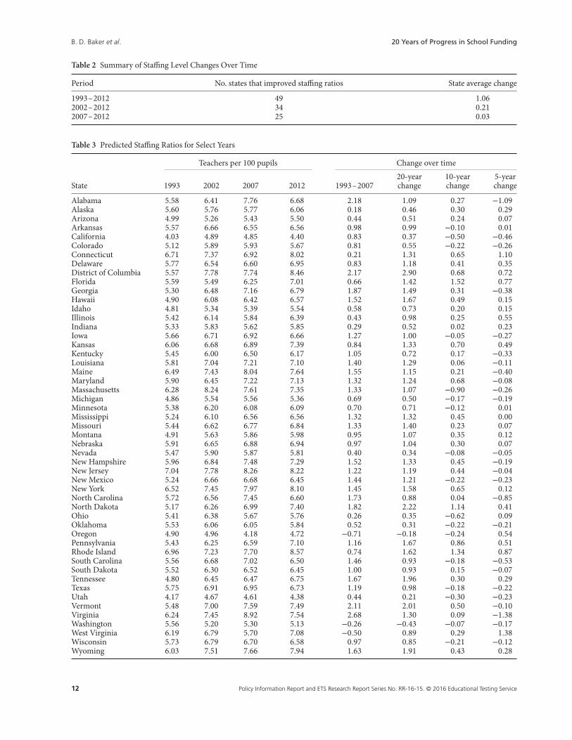
Table 2 summarizes changes to the numbers of teachers per 100 pupils over time. Over the entire 20-year period, nearlyall states increased numbers of staff per 100 pupils. The state average (unweighted) increase was approximately 1 additionalteacher per 100 pupils, moving from approximately 5.5 to approximately 6.5 total teachers per 100 pupils. Most of thosegains occurred prior to 2002. Over the past 10 years, state average staffing increases have been much more modest, andover the past 5 years, they have been nonexistent.
Table 3 displays state-by-state ratios of teachers per 100 pupils and changes in those ratios. States, includingAlabama and Virginia, appear to have reduced the number of teachers per 100 pupils by more than 1.0 (or by
0
5000
10000
0
5000
10000
1990 2000 2010 2020
1990 2000 2010 2020 1990 2000 2010 2020
Delaware Maryland New Jersey
New York Pennsylvania
State Aid Local Revenue
Federal Aid
year
Graphs by state_name0
2000
4000
6000
02000
4000
6000
1990 2000 2010 2020 1990 2000 2010 2020
Alabama Louisiana
Mississippi Texas
State Aid Local Revenue
Federal Aid
year
Graphs by state_name
0
5000
10000
0
5000
10000
1990 2000 2010 2020 1990 2000 2010 2020 1990 2000 2010 2020
Illinois Indiana Michigan
Minnesota Ohio Wisconsin
State Aid Local Revenue
Federal Aid
year
Graphs by state_name
05000
10000
15000
05000
10000
15000
1990 2000 2010 2020 1990 2000 2010 2020 1990 2000 2010 2020
Connecticut Maine Massachusetts
New Hampshire Rhode Island Vermont
State Aid Local Revenue
Federal Aid
year
Graphs by state_name
02000
4000
6000
8000
02000
4000
6000
8000
1990 2000 2010 2020
1990 2000 2010 2020
Idaho Oregon
Washington
State Aid Local Revenue
Federal Aid
year
Graphs by state_name
02000
4000
6000
8000
02000
4000
6000
8000
1990 2000 2010 2020 1990 2000 2010 2020 1990 2000 2010 2020
Iowa Kansas Missouri
Nebraska North Dakota South Dakota
State Aid Local Revenue
Federal Aid
year
Graphs by state_name
Figure 3 State revenue trends (excludes Alaska, Hawaii, and Nevada).
10 Policy Information Report and ETS Research Report Series No. RR-16-15. © 2016 Educational Testing Service

B. D. Baker et al. 20 Years of Progress in School Funding
05
00
01
00
00
05
00
01
00
00
1990 2000 2010 20201990 2000 2010 2020
Colorado Montana
Utah Wyoming
State Aid Local Revenue
Federal Aid
year
Graphs by state_name
05
00
01
00
00
05
00
01
00
00
1990 2000 2010 2020
1990 2000 2010 20201990 2000 2010 2020
Arkansas Kentucky Oklahoma
Tennessee West Virginia
State Aid Local Revenue
Federal Aid
year
Graphs by state_name
02
00
04
00
06
00
00
20
00
40
00
60
00
1990 2000 2010 2020
1990 2000 2010 20201990 2000 2010 2020
Florida Georgia North Carolina
South Carolina Virginia
State Aid Local Revenue
Federal Aid
year
Graphs by state_name
05
00
01
00
00
05
00
01
00
00
1990 2000 2010 2020
1990 2000 2010 2020
Arizona California
New Mexico
State Aid Local Revenue
Federal Aid
year
Graphs by state_name
Figure 3 Continued
5.50
5.60
5.70
5.80
5.90
6.00
6.10
6.20
6.30
6.40
6.50
6.60
Teac
her
s p
er 1
00 P
up
ils
Year
All Districts
K-12 Districts
K-12 Districs >2,000 Pupils
Figure 4 Teachers per 100 pupils over time.
approximately 13–16%) in recent years (2007–2012). Approximately half of states continued to increase numbersof teaching staff per 100 pupils over this time period. Notably, these figures change over time as a function of bothchanging numbers of staff and changing numbers of pupils. States with constant staffing but declining enrollments willshow increasing staffing ratios; states with increasing enrollment but no additional staff will show decreasing staffingratios.
Policy Information Report and ETS Research Report Series No. RR-16-15. © 2016 Educational Testing Service 11
B. D. Baker et al. 20 Years of Progress in School Funding
Table 2 Summary of Staffing Level Changes Over Time
Period No. states that improved staffing ratios State average change
1993–2012 49 1.062002–2012 34 0.212007–2012 25 0.03
Table 3 Predicted Staffing Ratios for Select Years
Teachers per 100 pupils Change over time
State 1993 2002 2007 2012 1993–200720-yearchange
10-yearchange
5-yearchange
Alabama 5.58 6.41 7.76 6.68 2.18 1.09 0.27 −1.09Alaska 5.60 5.76 5.77 6.06 0.18 0.46 0.30 0.29Arizona 4.99 5.26 5.43 5.50 0.44 0.51 0.24 0.07Arkansas 5.57 6.66 6.55 6.56 0.98 0.99 −0.10 0.01California 4.03 4.89 4.85 4.40 0.83 0.37 −0.50 −0.46Colorado 5.12 5.89 5.93 5.67 0.81 0.55 −0.22 −0.26Connecticut 6.71 7.37 6.92 8.02 0.21 1.31 0.65 1.10Delaware 5.77 6.54 6.60 6.95 0.83 1.18 0.41 0.35District of Columbia 5.57 7.78 7.74 8.46 2.17 2.90 0.68 0.72Florida 5.59 5.49 6.25 7.01 0.66 1.42 1.52 0.77Georgia 5.30 6.48 7.16 6.79 1.87 1.49 0.31 −0.38Hawaii 4.90 6.08 6.42 6.57 1.52 1.67 0.49 0.15Idaho 4.81 5.34 5.39 5.54 0.58 0.73 0.20 0.15Illinois 5.42 6.14 5.84 6.39 0.43 0.98 0.25 0.55Indiana 5.33 5.83 5.62 5.85 0.29 0.52 0.02 0.23Iowa 5.66 6.71 6.92 6.66 1.27 1.00 −0.05 −0.27Kansas 6.06 6.68 6.89 7.39 0.84 1.33 0.70 0.49Kentucky 5.45 6.00 6.50 6.17 1.05 0.72 0.17 −0.33Louisiana 5.81 7.04 7.21 7.10 1.40 1.29 0.06 −0.11Maine 6.49 7.43 8.04 7.64 1.55 1.15 0.21 −0.40Maryland 5.90 6.45 7.22 7.13 1.32 1.24 0.68 −0.08Massachusetts 6.28 8.24 7.61 7.35 1.33 1.07 −0.90 −0.26Michigan 4.86 5.54 5.56 5.36 0.69 0.50 −0.17 −0.19Minnesota 5.38 6.20 6.08 6.09 0.70 0.71 −0.12 0.01Mississippi 5.24 6.10 6.56 6.56 1.32 1.32 0.45 0.00Missouri 5.44 6.62 6.77 6.84 1.33 1.40 0.23 0.07Montana 4.91 5.63 5.86 5.98 0.95 1.07 0.35 0.12Nebraska 5.91 6.65 6.88 6.94 0.97 1.04 0.30 0.07Nevada 5.47 5.90 5.87 5.81 0.40 0.34 −0.08 −0.05New Hampshire 5.96 6.84 7.48 7.29 1.52 1.33 0.45 −0.19New Jersey 7.04 7.78 8.26 8.22 1.22 1.19 0.44 −0.04New Mexico 5.24 6.66 6.68 6.45 1.44 1.21 −0.22 −0.23New York 6.52 7.45 7.97 8.10 1.45 1.58 0.65 0.12North Carolina 5.72 6.56 7.45 6.60 1.73 0.88 0.04 −0.85North Dakota 5.17 6.26 6.99 7.40 1.82 2.22 1.14 0.41Ohio 5.41 6.38 5.67 5.76 0.26 0.35 −0.62 0.09Oklahoma 5.53 6.06 6.05 5.84 0.52 0.31 −0.22 −0.21Oregon 4.90 4.96 4.18 4.72 −0.71 −0.18 −0.24 0.54Pennsylvania 5.43 6.25 6.59 7.10 1.16 1.67 0.86 0.51Rhode Island 6.96 7.23 7.70 8.57 0.74 1.62 1.34 0.87South Carolina 5.56 6.68 7.02 6.50 1.46 0.93 −0.18 −0.53South Dakota 5.52 6.30 6.52 6.45 1.00 0.93 0.15 −0.07Tennessee 4.80 6.45 6.47 6.75 1.67 1.96 0.30 0.29Texas 5.75 6.91 6.95 6.73 1.19 0.98 −0.18 −0.22Utah 4.17 4.67 4.61 4.38 0.44 0.21 −0.30 −0.23Vermont 5.48 7.00 7.59 7.49 2.11 2.01 0.50 −0.10Virginia 6.24 7.45 8.92 7.54 2.68 1.30 0.09 −1.38Washington 5.56 5.20 5.30 5.13 −0.26 −0.43 −0.07 −0.17West Virginia 6.19 6.79 5.70 7.08 −0.50 0.89 0.29 1.38Wisconsin 5.73 6.79 6.70 6.58 0.97 0.85 −0.21 −0.12Wyoming 6.03 7.51 7.66 7.94 1.63 1.91 0.43 0.28
12 Policy Information Report and ETS Research Report Series No. RR-16-15. © 2016 Educational Testing Service

B. D. Baker et al. 20 Years of Progress in School Funding
AL
AK
AZ
AR
CA
CO
CT
DE
DC
FL
GA
HI
ID
IL
IN
IA
KS
KY
LA
ME
MD
MA
MI
MN
MS
MO
MT
NE
NV
NH
NJ
NM
NY
NC
ND
OHOK
OR
PA
RI
SCSD
TNTX
UT
VTVA
WA
WV
WI
WY
R2 = 0.4852
4
4.5
5
5.5
6
6.5
7
7.5
8
8.5
9
4000 6000 8000 10000 12000 14000 16000 18000
Tea
cher
s p
er 1
00 P
up
ils
Current Spending per Pupil (Constant 1999)
Spending Levels and Staffing Levels 2011-12
Figure 5 Spending levels and staffing levels, 2011–2012, showing line of best fit.
Table 4 Summary of Changes in Wage Competitiveness
Period No. states that increased wage competitiveness State mean change (%)
2000–2012 1 −122000–2007 3 −92007–2012 1 −8
The Relationship Between Staffing Levels and Funding Levels
As one might assume, more staffing per pupil requires more spending per pupil (unless, of course, wages are cut sub-stantially). Figure 5 conveys that states with higher per pupil spending tend, on average, to have more teachers per 100pupils; that is, on balance, across states, higher spending on schools is leveraged to increase staffing quantities. Perhapsmore important, however, is whether these increased overall staffing quantities translate into decreased class sizes, whereresearch literature has tended to point to more positive effects on student outcomes (see Baker, 2012; Schanzenbach, 2014).
Competitive Teacher Wages Over Time
Next, we summarize our competitive wage index over time for each state for 25- and 45-year-olds. Our index measuresthe ratio of predicted teacher wages to nonteacher wages for each state at constant age and degree level. Focusing on ages25 and 45 years allows us to examine the competitiveness of wages for those just entering the profession and again atmid-career.
Resource Input 2: Competitive wage ratio. Predicted annual wage of elementary and secondary teachers divided bypredicted wage of nonteachers working in the same state, with master’s degree, at specific ages.
Table 4 summarizes changes to the state average competitiveness of teacher wages over the past 12 years, and then forthe most recent 5 years. Wage competitiveness is expressed as a ratio of teacher wage to nonteacher wages. A ratio less than1.0 means that teachers earn less than comparable nonteachers. It is important to understand in this case that there are twomoving parts: teacher wages and nonteacher wages. Teacher wages can become more competitive if they remain relativelyconstant, but wages of others (at the same age and education level) decline. Teacher wages can become less competitiveeven if they appear to grow, but grow more slowly than wages in other sectors. Put simply, it is all relative, but it is therelative wage that matters.
Policy Information Report and ETS Research Report Series No. RR-16-15. © 2016 Educational Testing Service 13

B. D. Baker et al. 20 Years of Progress in School Funding
From 2000 to 2012, teacher wages in every state became less competitive based on our model, a finding that is consistentwith similar work by Allegretto, Corcoran, and Mishel (2011). It would appear that over the last 5 years, only in Iowa didteacher wages become marginally more competitive. Over the 12-year period, the state average (unweighted) reduction inwage competitiveness was 12%. Over the period from 2007 to 2012, the state average reduction in wage competitivenesswas 8%.
But, as can be seen in Table 5, these estimates tend to jump around, especially in low-population states such as Alaska.States with persistently noncompetitive teacher wages include Colorado and Arizona. Teacher wages have tended overtime to be more competitive in rural states (where nonteacher wages are not as high), including Montana and Wyoming.Average teacher wages in New York and Rhode Island have also tended to be more competitive.
Relationship Between Teacher Wages and Funding Levels
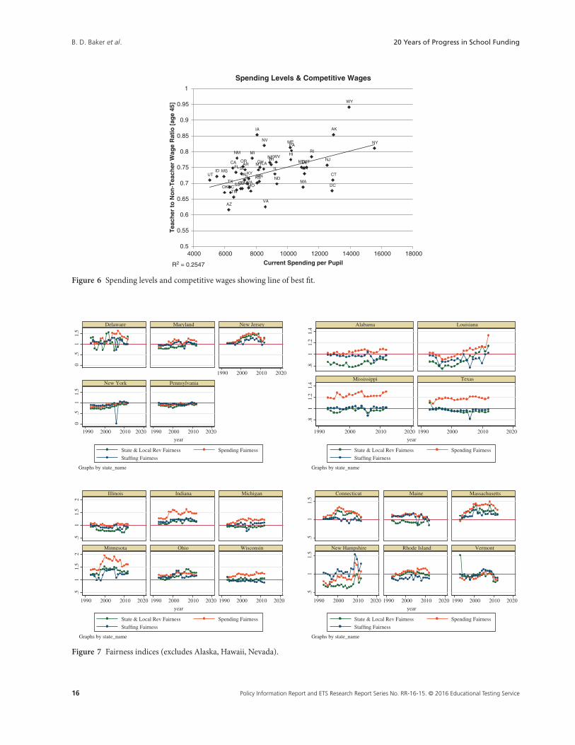
Figure 6 shows that, on average, states with higher current operating spending tend to have more competitive teacherwages. Coupled with previous analyses, this figure affirms the assumption that where current spending per pupil is higher,school districts have more competitively compensated staff. States including Utah, California, and Arizona suffer frompersistently low spending, leading to a combination of low staffing ratios and less competitive teacher wages. By contrast,higher spending states such as New York, New Jersey, and Wyoming tend to have both more competitive teacher wagesand higher staffing ratios. Again, these are state averages, which do not speak to whether money, teachers, or their wagesare distributed equitably across children in these states.
Spending and Staffing Fairness Over Time
Here, we begin exploring within-state distributions of resources across local public school districts by the concentrationof child poverty in those school districts. We explore our fairness ratio indicators:
Input Equity Indicator 1: Current spending fairness ratio. Predicted current spending per pupil for a district with 30%poverty divided by predicted current spending per pupil for a district with 0% poverty, for K–12 districts with 2,000or more students, in an average wage labor market.
• A current spending fairness ratio of 1.2 indicates that a high-poverty district is expected to have 20% higher perpupil spending than a low-poverty district, and the system is progressive.
• A current spending fairness ratio of 0.80 indicates that a high-poverty district is expected to have only 80% of thespending of a low-poverty district, and the system is regressive.
Input Equity Indicator 2: State and local revenue fairness ratio. Predicted state and local revenue per pupil for adistrict with 30% poverty divided by predicted state and local revenue per pupil for a district with 0% poverty,for K–12 districts with 2,000 or more students, in an average wage labor market.
• A state and local revenue fairness ratio of 1.2 indicates that a high-poverty district is expected to have 20% higherper pupil revenue than a low-poverty district, and the system is progressive.
• A state and local revenue fairness ratio of 0.80 indicates that a high-poverty district is expected to have only 80% ofthe revenue of a low-poverty district, and the system is regressive.
Input Equity Indicator 3: Staffing ratio (teachers per 100 pupils) fairness. Predicted staffing ratio for a district with30% poverty divided by predicted staffing ratio for a district with 0% poverty, for K–12 districts with 2,000 ormore students, in an average wage labor market
• A staffing ratio fairness ratio of 1.2 indicates that a high-poverty district is expected to have a 20% higher staffingratio than a low-poverty district, and the system is progressive.
• A staffing ratio fairness ratio of 0.80 indicates that a high-poverty district is expected to have 80% of the staffingratio of a low-poverty district, and the system is regressive.
Figure 7 tracks, side by side, the fairness indexes for (a) state and local revenue per pupil, (b) current spending perpupil, and (c) staffing ratios. When the revenue or spending fairness index is at the horizontal line (1.0), a local public
14 Policy Information Report and ETS Research Report Series No. RR-16-15. © 2016 Educational Testing Service

B. D. Baker et al. 20 Years of Progress in School Funding
Table 5 Teacher/Nonteacher Wage Ratios for Select Years
Wage competitivenessratio (teacher/nonteacher; %) Change over time (%)
State 2000 2002 2007 201212-yearchange
10-yearchange
5-yearchange
Alabama 83 83 77 71 −12 −12 −6Alaska 89 104 118 85 −4 −19 −33Arizona 79 74 70 62 −18 −13 −9Arkansas 82 84 82 74 −7 −10 −8California 79 82 82 75 −5 −7 −7Colorado 81 75 70 68 −13 −6 −2Connecticut 78 82 76 71 −7 −11 −5Delaware 82 87 83 75 −7 −13 −9District of Columbia 74 85 74 68 −7 −18 −6Florida 85 82 80 73 −11 −8 −6Georgia 76 76 74 68 −8 −8 −5Hawaii 95 83 81 77 −17 −6 −4Idaho 93 92 86 72 −21 −20 −13Illinois 77 78 79 73 −4 −5 −6Indiana 87 85 80 70 −17 −15 −10Iowa 86 87 83 85 −1 −2 3Kansas 87 80 77 70 −17 −10 −7Kentucky 84 80 78 71 −13 −9 −7Louisiana 78 78 79 75 −4 −3 −5Maine 90 79 90 81 −9 2 −9Maryland 80 77 78 75 −4 −2 −3Massachusetts 77 72 77 69 −8 −3 −8Michigan 93 88 94 78 −15 −10 −16Minnesota 84 80 75 71 −13 −10 −5Mississippi 86 81 78 72 −13 −9 −6Missouri 83 76 78 68 −16 −9 −11Montana 100 98 93 74 −26 −24 −19Nebraska 86 82 78 77 −10 −6 −2Nevada 93 85 84 82 −11 −3 −3New Hampshire 78 82 75 73 −5 −9 −2New Jersey 86 81 82 76 −10 −5 −6New Mexico 77 82 85 78 1 −4 −7New York 83 80 82 81 −2 1 −1North Carolina 80 79 75 67 −13 −12 −8North Dakota 87 86 77 70 −17 −17 −7Ohio 80 79 82 75 −5 −4 −7Oklahoma 80 78 76 67 −13 −11 −9Oregon 93 82 86 75 −17 −7 −11Pennsylvania 94 92 85 80 −13 −12 −5Rhode Island 92 87 94 78 −13 −8 −16South Carolina 86 89 77 73 −13 −16 −4South Dakota 82 88 78 68 −15 −21 −10Tennessee 86 74 76 66 −20 −9 −10Texas 77 78 73 69 −8 −9 −4Utah 99 93 79 71 −28 −22 −8Vermont 90 91 95 75 −15 −16 −20Virginia 76 75 72 63 −14 −12 −10Washington 79 78 74 69 −11 −9 −5West Virginia 89 79 79 77 −12 −3 −2Wisconsin 94 88 84 76 −18 −12 −8Wyoming 106 91 99 94 −12 3 −5
Policy Information Report and ETS Research Report Series No. RR-16-15. © 2016 Educational Testing Service 15
B. D. Baker et al. 20 Years of Progress in School Funding
AL
AK
AZ
ARCA
CO
CT
DE
DC
FL
GA
HI
IDIL
IN
IA
KSKY
LA
ME
MD
MA
MI
MNMS
MO
MT
NE
NV
NH
NJ
NM
NY
NC
ND
OH
OK
OR
PA
RI
SC
SD
TN
TX
UT
VT
VA
WA
WVWI
WY
R2 = 0.2547
0.5
0.55
0.6
0.65
0.7
0.75
0.8
0.85
0.9
0.95
1
4000 6000 8000 10000 12000 14000 16000 18000
Tea
cher
to
No
n-T
each
er W
age
Rat
io [
age
45]
Current Spending per Pupil
Spending Levels & Competitive Wages
Figure 6 Spending levels and competitive wages showing line of best fit.
0.5
11.5
0.5
11.5
1990 2000 2010 2020
1990 2000 2010 2020 1990 2000 2010 2020
Delaware Maryland New Jersey
New York Pennsylvania
State & Local Rev Fairness Spending Fairness
Staffing Fairness
year
Graphs by state_name
.81
1.2
1.4
.81
1.2
1.4
1990 2000 2010 2020 1990 2000 2010 2020
Alabama Louisiana
Mississippi Texas
State & Local Rev Fairness Spending Fairness
Staffing Fairness
year
Graphs by state_name
.51
1.5
2.5
11.5
2
1990 2000 2010 2020 1990 2000 2010 2020 1990 2000 2010 2020
Illinois Indiana Michigan
Minnesota Ohio Wisconsin
State & Local Rev Fairness Spending Fairness
Staffing Fairness
year
Graphs by state_name
.51
1.5
.51
1.5
1990 2000 2010 2020 1990 2000 2010 2020 1990 2000 2010 2020
Connecticut Maine Massachusetts
New Hampshire Rhode Island Vermont
State & Local Rev Fairness Spending Fairness
Staffing Fairness
year
Graphs by state_name
Figure 7 Fairness indices (excludes Alaska, Hawaii, Nevada).
16 Policy Information Report and ETS Research Report Series No. RR-16-15. © 2016 Educational Testing Service

B. D. Baker et al. 20 Years of Progress in School Funding
.81
1.2
1.4
1.6
.81
1.2
1.4
1.6
1990 2000 2010 2020
1990 2000 2010 2020
Idaho Oregon
Washington
State & Local Rev Fairness Spending FairnessStaffing Fairness
year
Graphs by state_name
.51
1.5
2.5
11.
52
1990 2000 2010 2020 1990 2000 2010 2020 1990 2000 2010 2020
Iowa Kansas Missouri
Nebraska North Dakota South Dakota
State & Local Rev Fairness Spending FairnessStaffing Fairness
year
Graphs by state_name
.51
1.5
2.5
11.
52
1990 2000 2010 2020 1990 2000 2010 2020
Colorado Montana
Utah Wyoming
State & Local Rev Fairness Spending FairnessStaffing Fairness
year
Graphs by state_name
.81
1.2
1.4
.81
1.2
1.4
1990 2000 2010 2020
1990 2000 2010 2020 1990 2000 2010 2020
Arkansas Kentucky Oklahoma
Tennessee West Virginia
State & Local Rev Fairness Spending FairnessStaffing Fairness
year
Graphs by state_name
.51
1.5
.51
1.5
1990 2000 2010 2020
1990 2000 2010 2020 1990 2000 2010 2020
Florida Georgia North Carolina
South Carolina Virginia
State & Local Rev Fairness Spending Fairness
Staffing Fairness
year
Graphs by state_name
.81
1.2
1.4
.81
1.2
1.4
1990 2000 2010 2020
1990 2000 2010 2020
Arizona California
New Mexico
State & Local Rev Fairness Spending Fairness
Staffing Fairness
year
Graphs by state_name
Figure 7 Continued
school district serving a high-poverty population would be expected to have comparable funding to a district serving alow-poverty population. When the revenue or spending fairness index rises above 1.0, higher poverty districts can beexpected to have more funding than lower poverty ones.
Figure 7 shows, for example, for New Jersey, that revenue and spending fairness climbed from approximately 1998to 2006, then leveled off and, more recently, plummeted back to a near-flat distribution. During that same time period,staffing ratio fairness also improved but has since regressed. The profile over time for Massachusetts is similar to thatof New Jersey but does not climb as high or fall as far. A state that has made significant gains, from regressive to pro-gressive, over time is Louisiana, with dramatically scaled-up funding to New Orleans area schools following HurricaneKatrina. By contrast, states including Pennsylvania and Illinois display persistently regressive patterns over the 20-yearperiod.
Policy Information Report and ETS Research Report Series No. RR-16-15. © 2016 Educational Testing Service 17

B. D. Baker et al. 20 Years of Progress in School Funding
Table 6 States Improving Funding Fairness
Initial fairness ratioamong improved states
PeriodNo. states that
improved fairness <0.95 0.95–1.05 >1.05
1993–2012 33 4 9 202002–2012 23 3 3 172007–2012 21 2 4 15
AL
AK
AZ
AR
CA
CO
CTDEDC
FL
GA
HI
ID
IL
IN
IA
KS
KY LA
MEMD
MAMI
MN
MSMO
MT
NE
NH
NJNM
NY
NC
ND
OH
OK
OR
PA
RI
SC
SD
TN
TX
UT
VT
VA
WAWV
WI
WY
R2 = 0.3633
0.8
0.9
1
1.1
1.2
1.3
1.4
1.5
1.6
0.8 1 1.2 1.4 1.6 1.8 2
Current Spending per Pupil Fairness Ratio
Spending Fairness & Staffing Fairness 2011-12
Tea
cher
s p
er 1
00 P
up
ils F
airn
ess
Rat
io
Figure 8 Spending fairness and staffing fairness, 2011–2012, showing line of best fit.
Numbers of Winners and Losers Over Time
So what, then, have been the consequences of the economic downturn for school spending fairness across states? That is,how have higher poverty districts been differentially affected when compared with lower poverty ones? Table 6 summa-rizes numbers of states where funding fairness improved over specific time periods over the past 20 years. Again, a fundingfairness ratio of 0.95 means that the district with 30% children in poverty10 has only 95% of the funding of a district with0% children in poverty. A fairness ratio of 1.05 indicates that a district with 30% poverty has 5% greater funding than adistrict with 0% poverty.
From 1993 to 2007 in particular, 40 states experienced increased funding levels in higher poverty districts relative tolower poverty ones. But in the 5 years that followed, 30 states reduced funding fairness, with some of the greatest reductionscoming in states that had previously experienced the greatest improvements, including New Jersey.
The Relationship Between Spending Fairness and Staffing Fairness
Figure 8 shows that, in 2012, states with more progressive distribution of current spending also had more progressivedistribution of staffing; that is, in states where higher poverty districts are able to spend more per pupil than lower povertydistricts, those higher poverty districts are able to leverage that spending to have more teaching staff per pupil than lowerpoverty districts.
Tables 7 and 8 clarify the connections from revenue to spending and spending to staffing ratios. Specifically, thelinear regression models in Table 7 ask whether changes to the level and distribution of state, local, and federalrevenues (a) are associated with differences across states and over time in spending fairness and (b) are associated
18 Policy Information Report and ETS Research Report Series No. RR-16-15. © 2016 Educational Testing Service

B. D. Baker et al. 20 Years of Progress in School Funding
Table 7 Cross-State Differences and Within-State Changes in Funding Fairness Translated to Spending Fairness
Within states, overtime (fixed effects)
Across and within states,over time (random effects)
Coefficient S.E. Coefficient S.E.
Fairness ratiosState 0.000 0.000 0.000 0.000Local 0.077 0.019* 0.080 0.019*
Federal 0.022 0.001* 0.022 0.001*
Revenue levels (ln)State 0.037 0.014* 0.033 0.014*
Local 0.003 0.015 −0.004 0.014Federal 0.063 0.014* 0.069 0.013*
Intercept 0.325 0.130* 0.371 0.130*
R2
Within 0.403 0.403Between 0.342 0.358Overall 0.311 0.320
*p< .05.
Table 8 Cross-State Differences and Within-State Changes in Spending Fairness Translated to Pupil/Teacher Ratio Fairness
Within states, overtime (fixed effects)
Across and within states,over time (random effects)
Coefficient S.E. Coefficient S.E.
Spending measuresSpending fairness 0.417 0.022* 0.432 0.020*
Constant 0.564 0.026* 0.546 0.026*
R2
Within 0.278 0.278Between 0.694 0.694Overall 0.572 0.572
Note. N = 50× 20 years.*p< .01.
specifically with changes over time in spending fairness (see Appendix C for model specification). Table 7 showsthat
• the level (amount) of state aid provided per pupil positively influences the fairness of current spending per pupil,• the fairness of local revenue (or degree of unfairness) influences the fairness of current spending per pupil, where
local revenues are less regressively distributed, current spending variation tends to be less regressive,• the level (amount) and fairness of federal revenues provided positively influence the fairness of current spending
per pupil.
In other words, as one might expect, state aid and federal revenue can improve the progressiveness of current spendingacross districts within states. These relationships hold not only across states but also over time. When state aid and federalaid are increased, fairness generally increases. But the degrees of disparity in local revenue raising still make a difference.
Table 8 provides additional evidence that the resulting differences in current spending fairness identified in Table 7lead to changes to the distribution of staffing. Like Table 7, Table 8 shows variations both across states and over time.Table 8 shows that as the spending fairness index rises over time, the staffing fairness index rises. Within states, over time,a 1.0 increase in spending fairness (which would involve doubling the ratio of spending in the highest poverty districtscompared to the lowest poverty ones) results, on average, in a 0.417 increase in the staffing ratio fairness index.
In other words, 20 years of data on all states (and all districts in them) validate that increased targeted funding to andspending in high-poverty districts within states lead to substantive increases in staffing ratios in those same districts,leading to more progressive state educational systems in terms of both funding and staffing. Notably, these relationshipswork in both directions.
Policy Information Report and ETS Research Report Series No. RR-16-15. © 2016 Educational Testing Service 19

B. D. Baker et al. 20 Years of Progress in School Funding
If increased targeted funding leads to increase targeted staffing, then so too does decreased targeted funding lead todecrease targeted staffing. As discussed earlier, over the past 5 years, and even 10, years, decreases, not increases, havebeen the norm. States have reduced targeted funding to high-need districts and thus reduced targeted staffing to thosesame districts.
Outcome Gaps Over Time
Finally, in this section, we begin exploring achievement gaps with respect to household income. Specifically, we exploreachievement gaps between children from low-income families and children from non-low-income families on the NAEP.But, as explained subsequently, we condition those achievement gaps on the income gaps between the two groups. Also,as a second indicator, we explore the “regressiveness” of NAEP score distributions across schools within states, that is, towhat extent are NAEP scores sensitive to differences in school-level child poverty?
Outcome Gap Indicator 1: Low-income achievement gap. Standardized difference in NAEP mean performance ofchildren from low-income families (children with free lunch) versus children from non-low-income families,corrected for differences in the mean income levels of the two groups.Outcome Gap Indicator 2: Income achievement effect. Statistical relationship across schools within states betweenschool-level concentration of children from low-income families (standardized within state) and school-levelexpected NAEP mean performance (conditioned on the average income of the families of students from low-incomefamilies in each state).11
A central assumption here is that states that have done a better job of targeting funding, and thus real resources, tohigher poverty settings over time would be more likely to show a reduction in achievement gaps by children’s familyincome status and reduction of the sensitivity of achievement measures to differences in school-level poverty; that is,more progressive resource allocation should lead to less regressive outcome distribution.
Numerous caveats are in order, and we attempt to address a few common concerns. First, achievement levels of childrenfrom low-income and non-low-income families across states depend on the income levels of these families, and so, too,do the gaps. As explained previously, we correct the achievement gaps for differences in income gaps. In some analyses,in which we focus specifically on achievement levels of low-income families, we correct those levels for income levels.A second set of concerns is more difficult to address: We have no way of knowing whether children from low-incomefamilies in the NAEP samples within states over time are attending predominantly low-income school districts in generalor more specifically high-poverty school districts as measured in our funding distribution measures. That is, if fundingdistributions are considered a “treatment” that might affect outcomes, we are not able, with NAEP outcome data, to identifyclearly the same “treatment” group.
We attempt to resolve this problem partially with our second approach to outcome disparity measurement, in whichwe relate school-level low-income concentrations with school-level outcomes. But even then, we do not know that thehigher and lower poverty schools are clearly aligned with higher and lower poverty districts (though the likelihood is inour favor). Finally, our NAEP data are generally biennial, not annual, and span the period from 1998 to 2013, making itharder to track changes over time, especially because we do not yet understand well the lag periods over which resourcechanges take hold and reveal themselves in student outcome changes.
Thus, as is the case with The Black–White Achievement Gap: When Progress Stopped (Barton & Coley, 2010), we areonly able herein to hypothesize about the connection between state policy contexts, resource distributions, and outcomedistributions, using scatterplots and regression analyses as descriptive tools to characterize relationships between inputsand outcomes across states. Unlike The Black–White Achievement Gap: When Progress Stopped, which focused only onnational average trends, by focusing on states over time, we are able to take more thorough steps to establish statisticalrelationships between state policy conditions—distributions of resources—and student outcome measures.
Figure 9 presents plots of our standardized adjusted outcome gap measures over time for all states. Among Mid-Atlanticstates, outcome gaps appear to decline in all but Pennsylvania, where outcome gaps remain larger than expected, givenincome gaps (above the red horizontal line). Notably, Pennsylvania does have the most persistently regressive funding dur-ing this period. In Gulf Coast states, outcome gaps decline in Louisiana, and initially in Texas, but remain flat and generallygreater than expected in the other states. Some states have consistently larger than expected achievement gaps, including
20 Policy Information Report and ETS Research Report Series No. RR-16-15. © 2016 Educational Testing Service

B. D. Baker et al. 20 Years of Progress in School Funding
Alabama, Illinois, and Wisconsin, whereas others have consistently smaller gaps, including Maine, North Dakota, andWest Virginia.
Resource Levels and Outcome Levels
Our big question is whether these gaps bear any relation to resource distribution differences across states. Figure 10 showsthe relationship between predicted staffing ratios by state and performance of children from low-income families (relativeto expectations, given their family income level) in Grade 4 for all states and all years; that is, this figure includes eachstate in each year. The figure shows a small positive correlation (see Figure 16) wherein states (by year) with higher staffingratios tend to have higher adjusted scale scores for fourth graders. What we cannot tell in Figure 10 is the extent to whichthe pattern is driven by (a) differences across states or (b) changes within states over time. Notably, because we have onlybiennial data for just longer than a decade, we simply do not have enough points within states over time to reveal clearpatterns or trends.
Figure 11 explores this same relationship using data from 2011 (the final matched year of NAEP and fiscal data as ofthe preparation of this report). Figure 11 shows similar relationships wherein states with higher staffing ratios do tendto have higher performance for children from low-income families. Using this approach, however, we cannot rule outthe possibility that state economic conditions provide simultaneously the opportunity to increase staffing ratios and theconditions that tend to lead to higher student outcomes; that is, some other contextual factors might be driving bothmeasures.
Figure 12 explores the cross-state (all years) relationship between relative competitive wages and low-income NAEPperformance. This relationship is somewhat weaker than the pupil-to-teacher ratio relationship, but perhaps not entirelyinconsequential. More competitive teacher wage states generally do not fall in the lower performance range. Figure 13shows this pattern across states for 2011 only, revealing little correlation.
-20
24
-20
24
1995 2000 2005 2010 2015
1995 2000 2005 2010 20151995 2000 2005 2010 2015
Delaware Maryland New Jersey
New York Pennsylvania
Adj. Gap Math 4 Adj. Gap Math 8
Adj. Gap Reading 4 Adj. Gap Reading 8
year
Graphs by state_name
-10
12
-10
12
1995 2000 2005 2010 20151995 2000 2005 2010 2015
Alabama Louisiana
Mississippi Texas
Adj. Gap Math 4 Adj. Gap Math 8
Adj. Gap Reading 4 Adj. Gap Reading 8
year
Graphs by state_name
-4-2
02
-4-2
02
1995 2000 2005 2010 20151995 2000 2005 2010 20151995 2000 2005 2010 2015
Illinois Indiana Michigan
Minnesota Ohio Wisconsin
Adj. Gap Math 4 Adj. Gap Math 8
Adj. Gap Reading 4 Adj. Gap Reading 8
year
Graphs by state_name
-4-2
02
-4-2
02
1995 2000 2005 2010 20151995 2000 2005 2010 20151995 2000 2005 2010 2015
Connecticut Maine Massachusetts
New Hampshire Rhode Island Vermont
Adj. Gap Math 4 Adj. Gap Math 8
Adj. Gap Reading 4 Adj. Gap Reading 8
year
Graphs by state_name
Figure 9 State trends in adjusted outcome gap measures.
Policy Information Report and ETS Research Report Series No. RR-16-15. © 2016 Educational Testing Service 21

B. D. Baker et al. 20 Years of Progress in School Funding
-20
24
-20
24
1995 2000 2005 2010 20151995 2000 2005 2010 2015
Alaska Idaho
Oregon Washington
Adj. Gap Math 4 Adj. Gap Math 8
Adj. Gap Reading 4 Adj. Gap Reading 8
year
Graphs by state_name
-20
2-2
02
1995 2000 2005 2010 20151995 2000 2005 2010 20151995 2000 2005 2010 2015
Iowa Kansas Missouri
Nebraska North Dakota South Dakota
Adj. Gap Math 4 Adj. Gap Math 8
Adj. Gap Reading 4 Adj. Gap Reading 8
year
Graphs by state_name
-2-1
01
2-2
-10
12
1995 2000 2005 2010 20151995 2000 2005 2010 2015
Colorado Montana
Utah Wyoming
Adj. Gap Math 4 Adj. Gap Math 8
Adj. Gap Reading 4 Adj. Gap Reading 8
year
Graphs by state_name
-4-2
02
-4-2
02
1995 2000 2005 2010 2015
1995 2000 2005 2010 20151995 2000 2005 2010 2015
Arkansas Kentucky Oklahoma
Tennessee West Virginia
Adj. Gap Math 4 Adj. Gap Math 8
Adj. Gap Reading 4 Adj. Gap Reading 8
year
Graphs by state_name
-2-1
01
2-2
-10
12
1995 2000 2005 2010 2015
1995 2000 2005 2010 20151995 2000 2005 2010 2015
Florida Georgia North Carolina
South Carolina Virginia
Adj. Gap Math 4 Adj. Gap Math 8
Adj. Gap Reading 4 Adj. Gap Reading 8
year
Graphs by state_name
-20
2-2
02
1995 2000 2005 2010 20151995 2000 2005 2010 2015
Arizona California
Nevada New Mexico
Adj. Gap Math 4 Adj. Gap Math 8
Adj. Gap Reading 4 Adj. Gap Reading 8
year
Graphs by state_name
Figure 9 Continued
Resource Distributions and Outcome Distributions
Here, we move from looking at resources and the level of performance of children from low-income families to resourcedistributions and achievement gaps. Again, the assumption is that states in which staffing ratios are significantly higher(progressive) in higher poverty settings may be more likely to show smaller income-based achievement gaps, after adjust-ing for income gaps; that is, targeted staffing increases can help reduce achievement gaps. Figure 14 provides evidence ofsome pattern across all states over all years. States with higher staffing ratio fairness indexes, indicating that staffing ratiostend to be higher in higher poverty districts, also tend to have lower than expected NAEP achievement gaps in Grade 8.Figure 15 tells a similar story for Grade 4.
22 Policy Information Report and ETS Research Report Series No. RR-16-15. © 2016 Educational Testing Service

B. D. Baker et al. 20 Years of Progress in School Funding
-4-2
02
4
4 6 8 10
Teachers per 100 Pupils
Adj. Math 4 Low Income Adj. Reading 4 Low Income
All Years
Teachers per 100 Level & Adj. NAEP Low Income
Ad
j.N
AE
P -
Lo
w I
nco
me
Figure 10 Teachers per 100 level and adjusted National Assessment of Educational Progress low income, all years. Correlation(Math= .24, Reading= .25).
AL
NC
AR
CT
MDTX
AZ
MA
NE
RI
OK
MI
VT
MO
VA
IDSD
FL
SC
NDIN KS
MN
UT
DE
MT
KY WY
NJ
NM
IA
PA
LA
NY
OH
NH
GA
HI TN
WA
IL
MS
COWI
OR
ME
WV
CA
ALNCAR
CT
MD
TX
AZ
MA
NE
RIOK
MI
VT
MO
VAID
SD
FL
SC
ND
INKS
MN
UT
DEMT
KY
WYNJ
NM
IA
PA
LA
NYOH
NH
GA
HI
TNWA IL
MS
CO
WIOR
ME
WV
CA
-2-1
01
2
Ad
j. N
AE
P -
Lo
w I
nco
me
4 5 6 7 8Teachers per 100 Pupils
Adj. Math 4 Low Income Adj. Reading 4 Low Income
2011
Teachers per 100 Level & Adj. NAEP Low Income
Figure 11 Teachers per 100 level and adjacent National Assessment of Educational Progress low income, 2011. Correlation (Math= .30,Reading= .44).
Figure 16 summarizes the correlations of our outcome measures for all grades and subjects with our salary paritymeasures (a level indicator) and for our staffing ratio level and fairness (distribution) measures. Again, our outcomemeasures include the following:
Outcome Level Indicator 1: Low-income students’ performance level. State average performance of children from lowincome families (receiving free lunch), conditioned on the average income levels of students from low-incomefamilies in the state and expressed as standardized differences between the expected performance level (given incomelevels) and actual performance levels.Outcome Gap Indicator 1: Low-income achievement gap. State average achievement gaps between children fromlow-income families and children from non-low-income families adjusted for the difference (gap) in income betweenfamilies of low income and non-low income and expressed as standardized differences between the expectedachievement gap and the actual gap.Outcome Gap Indicator 2: Income achievement effect. Within-state ratio of expected NAEP performance inhigh-poverty school (+2 S.D.) to low-poverty school (−2 S.D.), adjusted for the difference (gap) in income betweenfamilies of low income and non-low income (see note 11).
Policy Information Report and ETS Research Report Series No. RR-16-15. © 2016 Educational Testing Service 23

B. D. Baker et al. 20 Years of Progress in School Funding
-4-2
02
4
Ad
j. N
AE
P -
Lo
w I
nco
me
.7 .8 .9 1 1.1 1.2
Wage Parity at 25
Adj. Math 8 Low Income Adj. Reading 8 Low Income
All Years
Teacher Wages & Adj. NAEP Low Income
Figure 12 Teacher wages and adjusted National Assessment of Educational Progress low income, all years. Correlation (Math= .12,Reading= .16).
AL
NC
AR
CT
MD
TX
AZ
MA
NE
RI
OK
MI
VT
MO
VA
ID
SD
FL
SC
ND
INKSMN
UT
DE
MT
KYWY
NJ
NM
IA
PALANY
OHNH
GA
HITN
WA IL
MS
CO
WI
OR
ME
WV
CA
AL
NC
AR
CT
MD
TX
AZ
MA
NERI
OKMI
VT
MO
VA
ID
SD
FL
SC
ND
INKS
MN
UT
DE
MTKY
WY
NJ
NM
IA
PA
LA
NY
OH
NH
GA
HI
TN
WAIL
MS
CO
WI
OR
ME
WV
CA
-2-1
01
2
Adj.
NA
EP
- L
ow
Incom
e
.7 .8 .9 1
Wage Parity at 25
Adj. Math 8 Low Income Adj. Reading 8 Low Income
2011
Teacher Wages & Adj. NAEP Low Income
Figure 13 Teacher wages and adjusted National Assessment of Educational Progress low income, 2011. Correlation (Math= .15, Read-ing= .15).
All correlations, except those shaded more lightly, are statistically significant, p< .05. Blue bars show the correlationsbetween our staffing ratio level indicator and outcome measures (levels and gaps). That indicator has a small to no cor-relation (nonsignificant shaded bars) with our achievement gap measures but does have a consistently modest positivecorrelation with our low-family-income students’ achievement level indicator. Staffing levels also have modest positiverelationships with our achievement progressiveness measures, where higher staffing levels are associated with higher ratiosof performance in low-income schools to that of higher income schools; that is, in states where staffing ratios are higher,lower-family-income students tend to be performing better.
The red bars indicate the relationship between our staffing ratio fairness indicators and each outcome measure. Here,we see that the staffing fairness ratio is modestly negatively correlated with our achievement gap measure; that is, wherestaffing ratios are higher in higher poverty settings, achievement gaps are lower. The inverse is also true: Where staffing fair-ness wanes, achievement gaps are larger. Correlations tend to be strongest between staffing fairness and outcome fairness,using our outcome regressiveness ratio.
Green bars show correlations for salary parity indexes for 45-year-olds. Again, this is a level indicator, indicating therelative competitiveness of teacher salaries to the salaries of similarly educated, same-age nonteachers working in thesame state. The correlations, though smaller in magnitude, do fall in the expected direction. States with more competitiveteacher wages have (a) smaller achievement gaps (than expected) and (b) higher mean scale scores (than expected) for
24 Policy Information Report and ETS Research Report Series No. RR-16-15. © 2016 Educational Testing Service
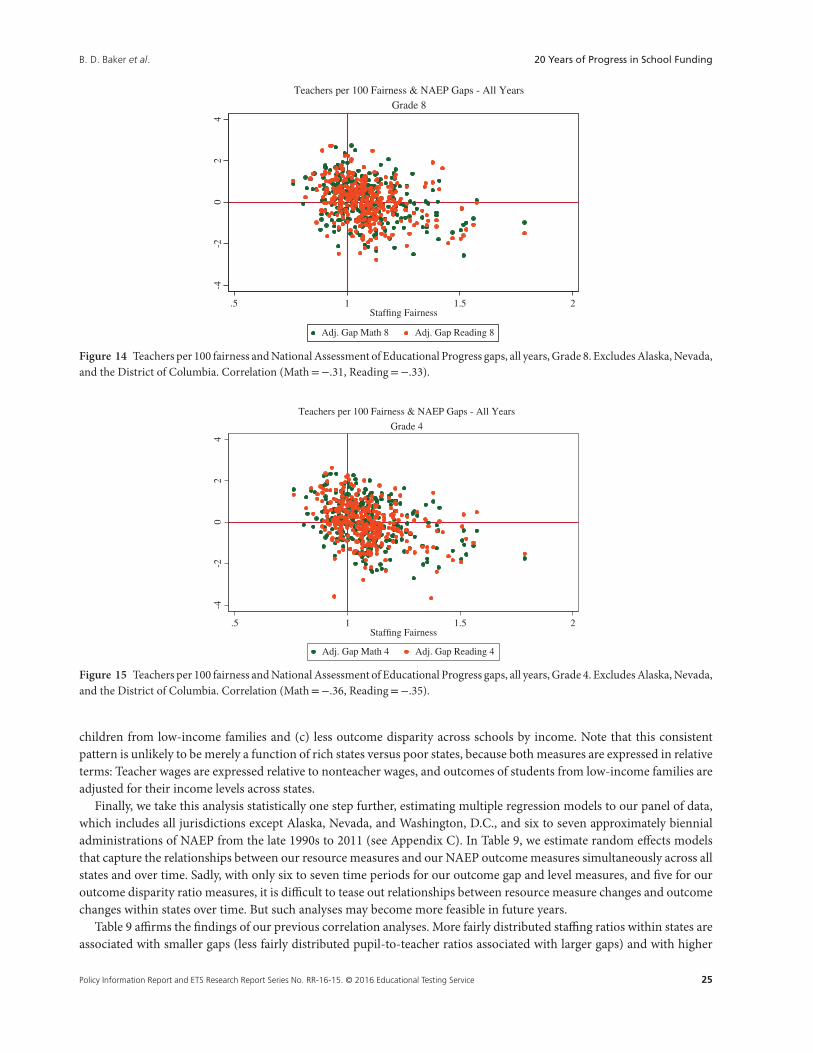
B. D. Baker et al. 20 Years of Progress in School Funding
-4-2
02
4
.5 1 1.5 2Staffing Fairness
Adj. Gap Math 8 Adj. Gap Reading 8
Grade 8
Teachers per 100 Fairness & NAEP Gaps - All Years
Figure 14 Teachers per 100 fairness and National Assessment of Educational Progress gaps, all years, Grade 8. Excludes Alaska, Nevada,and the District of Columbia. Correlation (Math=−.31, Reading=−.33).
-4-2
02
4
.5 1 1.5 2Staffing Fairness
Adj. Gap Math 4 Adj. Gap Reading 4
Grade 4
Teachers per 100 Fairness & NAEP Gaps - All Years
Figure 15 Teachers per 100 fairness and National Assessment of Educational Progress gaps, all years, Grade 4. Excludes Alaska, Nevada,and the District of Columbia. Correlation (Math=−.36, Reading=−.35).
children from low-income families and (c) less outcome disparity across schools by income. Note that this consistentpattern is unlikely to be merely a function of rich states versus poor states, because both measures are expressed in relativeterms: Teacher wages are expressed relative to nonteacher wages, and outcomes of students from low-income families areadjusted for their income levels across states.
Finally, we take this analysis statistically one step further, estimating multiple regression models to our panel of data,which includes all jurisdictions except Alaska, Nevada, and Washington, D.C., and six to seven approximately biennialadministrations of NAEP from the late 1990s to 2011 (see Appendix C). In Table 9, we estimate random effects modelsthat capture the relationships between our resource measures and our NAEP outcome measures simultaneously across allstates and over time. Sadly, with only six to seven time periods for our outcome gap and level measures, and five for ouroutcome disparity ratio measures, it is difficult to tease out relationships between resource measure changes and outcomechanges within states over time. But such analyses may become more feasible in future years.
Table 9 affirms the findings of our previous correlation analyses. More fairly distributed staffing ratios within states areassociated with smaller gaps (less fairly distributed pupil-to-teacher ratios associated with larger gaps) and with higher
Policy Information Report and ETS Research Report Series No. RR-16-15. © 2016 Educational Testing Service 25

B. D. Baker et al. 20 Years of Progress in School Funding
0.2
5
0.0
5
0.2
4
0.0
4
(0.1
8)
(0.0
2)
(0.1
4)
0.0
4
0.2
8
0.2
0
0.2
5
0.1
7
0.3
3
0.2
4
0.3
9
0.2
9
(0.3
5)
(0.3
3)
(0.3
6)
(0.3
1)
0.3
8
0.4
3
0.3
7
0.4
3
0.1
1
0.0
1
0.1
4
0.0
4
(0.1
2)
(0.1
4)
(0.0
9)
(0.1
6)
0.1
3
0.1
6
0.0
8
0.1
2
Readin
g 4
Readin
g 8
Math
4
Math
8
Readin
g 4
Readin
g 8
Math
4
Math
8
Readin
g 4
Readin
g 8
Math
4
Math
8
Low Inc. Performance Level Low Inc. Achievement Gap Income Achievement Effect
Teachers per 100 Pupils Teachers per 100 Pupils Fairness Salary Parity (45)
Figure 16 Correlations between resource measures and adjusted National Assessment of Educational Progress measures (all statesand all years). Performance for children qualified for free lunch (<130% income threshold for poverty), adjusted for income differencesacross states, and gap between scale scores for children not qualified for free lunch (>130% income threshold for poverty) and childrenqualified for free lunch (<130% income threshold for poverty), adjusted for differences in income gaps across states. Excludes Alaska,Nevada, and the District of Columbia.
scores for children from low-income families. These patterns are relatively consistent across tests (except for eighth-grademathematics on our alternative outcome disparity measure). In fourth-grade reading, higher staffing levels are also asso-ciated with smaller achievement gaps.
Linkages between competitive wage levels, low-income performance levels, and achievement gaps are less clearwhen similar regression models are estimated. All coefficients are in the expected direction, and some are statisticallysignificant at various thresholds. Competitive wages for 25-year-old teachers are positively associated with (a) low-income fourth-grade mathematics achievement, p< .10; (b) low-income fourth-grade reading achievement, p< .05;(c) low-income eighth-grade mathematics achievement, p< .05; and (d) low-income eighth-grade reading achievement(ns). More competitive wages for 25-year-old teachers are associated with smaller achievement gaps for (a) fourth-grade mathematics (ns); (b) fourth-grade reading (ns); (c) eighth-grade mathematics, p< .10; and (d) eighth-gradereading (ns).
What Does It All Mean?
The analyses presented here validate the conclusion that variations in available revenues and expenditures are associatedwith variations in children’s access to real resources, as measured by the competitiveness of the wages paid to their teachersand by pupil-to-teacher ratios and class sizes. Variations in the levels and distributions of real resources are, in turn,associated with the levels and distributions of student outcomes across states:
• States that apply more effort—spending a greater share of their fiscal capacity on schools—spend more generallyon schools.
• These higher spending levels translate into higher statewide staffing levels—more teaching staff per pupil.• These higher spending levels translate into more competitive statewide teacher wages.
26 Policy Information Report and ETS Research Report Series No. RR-16-15. © 2016 Educational Testing Service
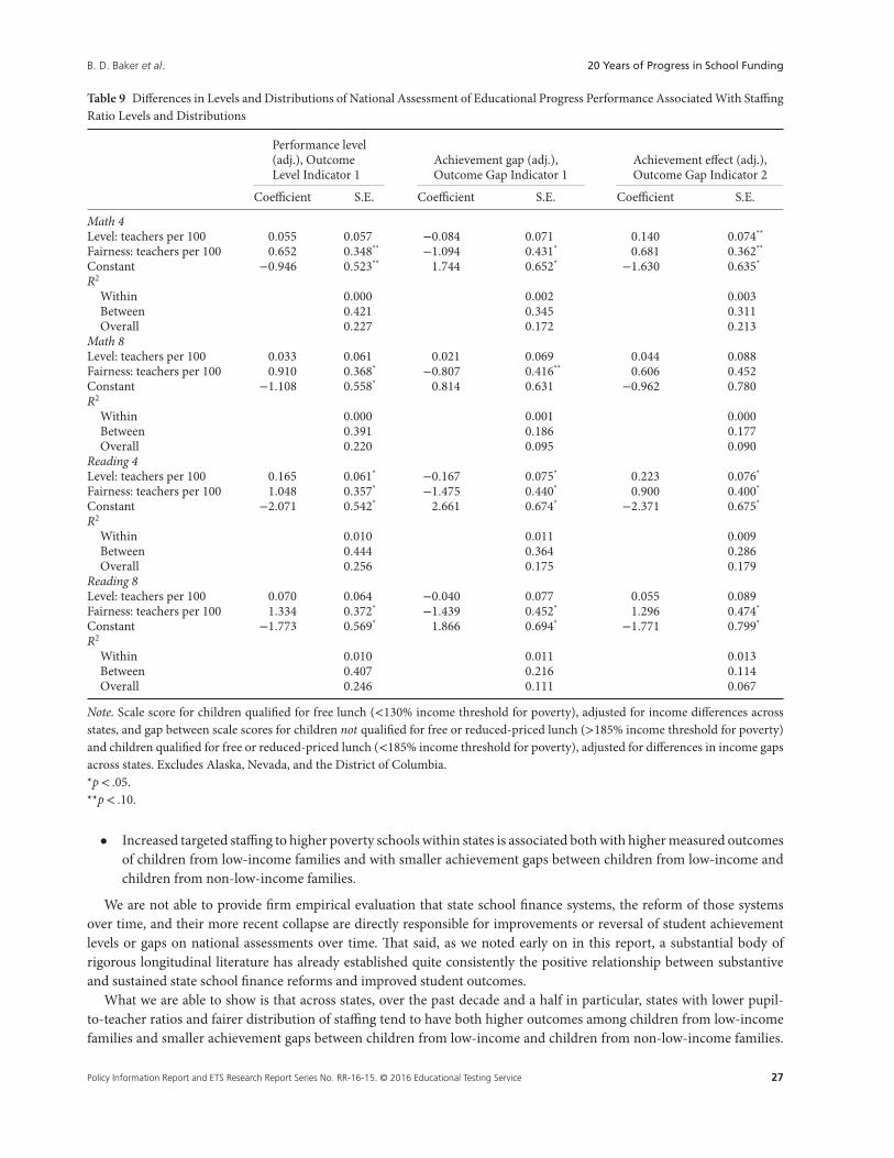
B. D. Baker et al. 20 Years of Progress in School Funding
Table 9 Differences in Levels and Distributions of National Assessment of Educational Progress Performance Associated With StaffingRatio Levels and Distributions
Performance level(adj.), OutcomeLevel Indicator 1
Achievement gap (adj.),Outcome Gap Indicator 1
Achievement effect (adj.),Outcome Gap Indicator 2
Coefficient S.E. Coefficient S.E. Coefficient S.E.
Math 4Level: teachers per 100 0.055 0.057 −0.084 0.071 0.140 0.074**
Fairness: teachers per 100 0.652 0.348** −1.094 0.431* 0.681 0.362**
Constant −0.946 0.523** 1.744 0.652* −1.630 0.635*
R2
Within 0.000 0.002 0.003Between 0.421 0.345 0.311Overall 0.227 0.172 0.213
Math 8Level: teachers per 100 0.033 0.061 0.021 0.069 0.044 0.088Fairness: teachers per 100 0.910 0.368* −0.807 0.416** 0.606 0.452Constant −1.108 0.558* 0.814 0.631 −0.962 0.780R2
Within 0.000 0.001 0.000Between 0.391 0.186 0.177Overall 0.220 0.095 0.090
Reading 4Level: teachers per 100 0.165 0.061* −0.167 0.075* 0.223 0.076*
Fairness: teachers per 100 1.048 0.357* −1.475 0.440* 0.900 0.400*
Constant −2.071 0.542* 2.661 0.674* −2.371 0.675*
R2
Within 0.010 0.011 0.009Between 0.444 0.364 0.286Overall 0.256 0.175 0.179
Reading 8Level: teachers per 100 0.070 0.064 −0.040 0.077 0.055 0.089Fairness: teachers per 100 1.334 0.372* −1.439 0.452* 1.296 0.474*
Constant −1.773 0.569* 1.866 0.694* −1.771 0.799*
R2
Within 0.010 0.011 0.013Between 0.407 0.216 0.114Overall 0.246 0.111 0.067
Note. Scale score for children qualified for free lunch (<130% income threshold for poverty), adjusted for income differences acrossstates, and gap between scale scores for children not qualified for free or reduced-priced lunch (>185% income threshold for poverty)and children qualified for free or reduced-priced lunch (<185% income threshold for poverty), adjusted for differences in income gapsacross states. Excludes Alaska, Nevada, and the District of Columbia.*p< .05.**p< .10.
• Increased targeted staffing to higher poverty schools within states is associated both with higher measured outcomesof children from low-income families and with smaller achievement gaps between children from low-income andchildren from non-low-income families.
We are not able to provide firm empirical evaluation that state school finance systems, the reform of those systemsover time, and their more recent collapse are directly responsible for improvements or reversal of student achievementlevels or gaps on national assessments over time. That said, as we noted early on in this report, a substantial body ofrigorous longitudinal literature has already established quite consistently the positive relationship between substantiveand sustained state school finance reforms and improved student outcomes.
What we are able to show is that across states, over the past decade and a half in particular, states with lower pupil-to-teacher ratios and fairer distribution of staffing tend to have both higher outcomes among children from low-incomefamilies and smaller achievement gaps between children from low-income and children from non-low-income families.
Policy Information Report and ETS Research Report Series No. RR-16-15. © 2016 Educational Testing Service 27
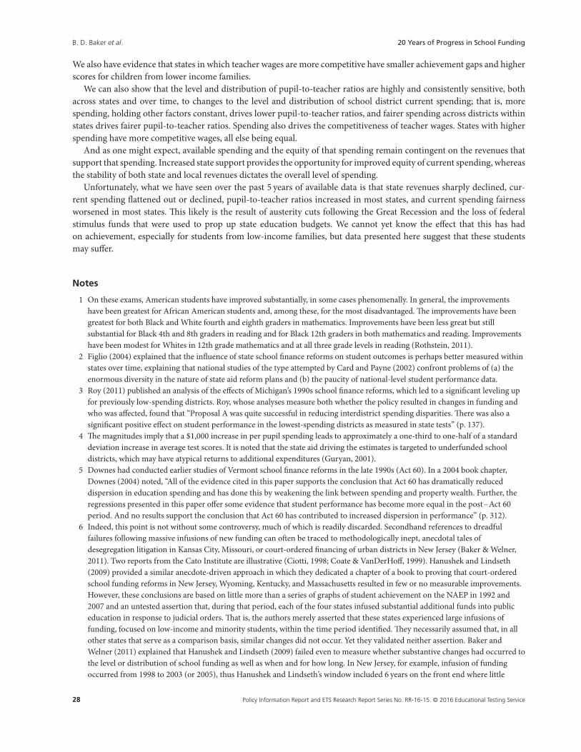
B. D. Baker et al. 20 Years of Progress in School Funding
We also have evidence that states in which teacher wages are more competitive have smaller achievement gaps and higherscores for children from lower income families.
We can also show that the level and distribution of pupil-to-teacher ratios are highly and consistently sensitive, bothacross states and over time, to changes to the level and distribution of school district current spending; that is, morespending, holding other factors constant, drives lower pupil-to-teacher ratios, and fairer spending across districts withinstates drives fairer pupil-to-teacher ratios. Spending also drives the competitiveness of teacher wages. States with higherspending have more competitive wages, all else being equal.
And as one might expect, available spending and the equity of that spending remain contingent on the revenues thatsupport that spending. Increased state support provides the opportunity for improved equity of current spending, whereasthe stability of both state and local revenues dictates the overall level of spending.
Unfortunately, what we have seen over the past 5 years of available data is that state revenues sharply declined, cur-rent spending flattened out or declined, pupil-to-teacher ratios increased in most states, and current spending fairnessworsened in most states. This likely is the result of austerity cuts following the Great Recession and the loss of federalstimulus funds that were used to prop up state education budgets. We cannot yet know the effect that this has hadon achievement, especially for students from low-income families, but data presented here suggest that these studentsmay suffer.
Notes
1 On these exams, American students have improved substantially, in some cases phenomenally. In general, the improvementshave been greatest for African American students and, among these, for the most disadvantaged. The improvements have beengreatest for both Black and White fourth and eighth graders in mathematics. Improvements have been less great but stillsubstantial for Black 4th and 8th graders in reading and for Black 12th graders in both mathematics and reading. Improvementshave been modest for Whites in 12th grade mathematics and at all three grade levels in reading (Rothstein, 2011).
2 Figlio (2004) explained that the influence of state school finance reforms on student outcomes is perhaps better measured withinstates over time, explaining that national studies of the type attempted by Card and Payne (2002) confront problems of (a) theenormous diversity in the nature of state aid reform plans and (b) the paucity of national-level student performance data.
3 Roy (2011) published an analysis of the effects of Michigan’s 1990s school finance reforms, which led to a significant leveling upfor previously low-spending districts. Roy, whose analyses measure both whether the policy resulted in changes in funding andwho was affected, found that “Proposal A was quite successful in reducing interdistrict spending disparities. There was also asignificant positive effect on student performance in the lowest-spending districts as measured in state tests” (p. 137).
4 The magnitudes imply that a $1,000 increase in per pupil spending leads to approximately a one-third to one-half of a standarddeviation increase in average test scores. It is noted that the state aid driving the estimates is targeted to underfunded schooldistricts, which may have atypical returns to additional expenditures (Guryan, 2001).
5 Downes had conducted earlier studies of Vermont school finance reforms in the late 1990s (Act 60). In a 2004 book chapter,Downes (2004) noted, “All of the evidence cited in this paper supports the conclusion that Act 60 has dramatically reduceddispersion in education spending and has done this by weakening the link between spending and property wealth. Further, theregressions presented in this paper offer some evidence that student performance has become more equal in the post–Act 60period. And no results support the conclusion that Act 60 has contributed to increased dispersion in performance” (p. 312).
6 Indeed, this point is not without some controversy, much of which is readily discarded. Secondhand references to dreadfulfailures following massive infusions of new funding can often be traced to methodologically inept, anecdotal tales ofdesegregation litigation in Kansas City, Missouri, or court-ordered financing of urban districts in New Jersey (Baker & Welner,2011). Two reports from the Cato Institute are illustrative (Ciotti, 1998; Coate & VanDerHoff, 1999). Hanushek and Lindseth(2009) provided a similar anecdote-driven approach in which they dedicated a chapter of a book to proving that court-orderedschool funding reforms in New Jersey, Wyoming, Kentucky, and Massachusetts resulted in few or no measurable improvements.However, these conclusions are based on little more than a series of graphs of student achievement on the NAEP in 1992 and2007 and an untested assertion that, during that period, each of the four states infused substantial additional funds into publiceducation in response to judicial orders. That is, the authors merely asserted that these states experienced large infusions offunding, focused on low-income and minority students, within the time period identified. They necessarily assumed that, in allother states that serve as a comparison basis, similar changes did not occur. Yet they validated neither assertion. Baker andWelner (2011) explained that Hanushek and Lindseth (2009) failed even to measure whether substantive changes had occurred tothe level or distribution of school funding as well as when and for how long. In New Jersey, for example, infusion of fundingoccurred from 1998 to 2003 (or 2005), thus Hanushek and Lindseth’s window included 6 years on the front end where little
28 Policy Information Report and ETS Research Report Series No. RR-16-15. © 2016 Educational Testing Service

B. D. Baker et al. 20 Years of Progress in School Funding
change occurred. Kentucky reforms had largely faded by the mid to late 1990s, yet Hanushek and Lindseth measured postreformeffects in 2007. Furthermore, in New Jersey, funding was infused into approximately 30 specific districts, but Hanushek andLindseth explored overall changes to outcomes among low-income children and minorities using NAEP data, where some ofthese children attended the districts receiving additional support, but many did not. In short, the slipshod comparisonsHanushek and Lindseth made provided no reasonable basis for asserting either the success or failure of state school financereforms. Hanushek (2006) went so far as to title the book Courting Failure: How School Finance Lawsuits Exploit Judges’ GoodIntentions and Harm Our Children. The premise that additional funding for schools often leveraged toward class size reduction,additional course offerings, or increased teacher salaries causes harm to children is, on its face, absurd. And the book, whichimplies as much in its title, never once validated that such reforms ever do cause harm. Rather, the title is little more than amanipulative attempt to convince the noncritical spectator who never gets past the book’s cover to fear that school financereforms might somehow harm children. The book also included two examples of a type of analysis that occurred with somefrequency in the mid-2000s that also had the intent of showing that school funding does not matter. These studies wouldcherry-pick anecdotal information on either or both (a) poorly funded schools that have high outcomes or (b) well-fundedschools that have low outcomes (see Evers & Clopton, 2006; Walberg, 2006). In an equally problematic analysis, Neymotin (2010)set out to show that massive court-ordered infusions of funding in Kansas following Montoy v. Kansas led to no substantiveimprovements in student outcomes. However, Neymotin evaluated changes in school funding from 1997 to 2006, but the firstadditional funding infused following the January 2005 Supreme Court decision occurred in the 2005–2006 school year, the endpoint of Neymotin’s outcome data. Greene and Trivitt (2008) presented a study in which they claimed to show thatcourt-ordered school finance reforms led to no substantive improvements in student outcomes. However, the authors tested onlywhether the presence of a court order is associated with changes in outcomes and never once measured whether substantiveschool finance reforms followed the court order, but they still expressed the conclusion that court-ordered funding increases haveno effect.
7 Although often treated as a newer approach to equity analysis than measuring pure fiscal inputs, equity evaluations of realresources predate modern school finance equity, often being used, for example, to evaluate the uniformity of segregated Blackand White schools operating in the pre-Brown, separate-but-equal era (Baker & Green, 2009b).
8 As per the court’s declaration in Rose v. Council for Better Educ., Inc. (1989), “an efficient system of education must have as its goalto provide each and every child with at least the seven following capacities: (i) sufficient oral and written communication skills toenable students to function in a complex and rapidly changing civilization; (ii) sufficient knowledge of economic, social, andpolitical systems to enable the student to make informed choices; (iii) sufficient understanding of governmental processes toenable the student to understand the issues that affect his or her community, state, and nation; (iv) sufficient self-knowledge andknowledge of his or her mental and physical wellness; (v) sufficient grounding in the arts to enable each student to appreciate hisor her cultural and historical heritage; (vi) sufficient training or preparation for advanced training in either academic orvocational fields so as to enable each child to choose and pursue life work intelligently; and (vii) sufficient levels of academic orvocational skills to enable public school students to compete favorably with their counterparts in surrounding states, inacademics or in the job market.” See also Thro (2009).
9 Where our standardized, expected gap measure is the standardized residual of the regression NAEP Income AchievementGapst = b0 + b1ACS Income Gapst + b2Year+ e for each state (s) in year (t).
10 Census poverty rate, where 30% rate is equivalent to approximately 80% free or reduced-priced lunch.11 Here, we take the standardized (z-score) NAEP estimate for each school (standardized around state mean) and standardized
low-income share for each school (z-score around state mean) and estimate the following regression: NAEP SchoolStandardized= b0 + b1Poverty Standardized+ b2State+ b3State×Poverty Standardized+ e. Next, we use this regression togenerate predicted values of NAEP for high-poverty (2 S.D.s above state mean) and low-poverty (2 S.D.s below state mean)schools in each state and year. We then calculate the ratio of the NAEP for high-poverty to low-poverty schools. Thesevalues are invariably below 1.0, and positive change in this value indicates reduction income-related disparity in NAEP acrossschools.
References
Allegretto, S. A., Corcoran, S. P., & Mishel, L. R. (2008). The teaching penalty: Teacher pay losing ground. Washington, DC: EconomicPolicy Institute.
Allegretto, S. A., Corcoran, S. P., & Mishel, L. (2011). The teaching penalty: An update through 2010 (EPI Issue Brief No. 298). Washing-ton, DC: Economic Policy Institute.
American Institutes for Research. (n.d.). National longitudinal school-level state assessment score database [Data set]. Retrieved fromhttp://www.schooldata.org/DataFiles/tabid/65/Default.aspx
Policy Information Report and ETS Research Report Series No. RR-16-15. © 2016 Educational Testing Service 29
B. D. Baker et al. 20 Years of Progress in School Funding
Baker, B. D. (2012). Revisiting the age-old question: Does money matter in education? Washington, DC: Albert Shanker Institute.Baker, B. D. (2014). Evaluating the recession’s impact on equity and adequacy of state school finance systems. Education Policy Analysis
Archives, 22(91), 1–33. Retrieved from http://epaa.asu.edu/ojs/article/view/1590Baker, B. D., Farrie, D., & Sciarra, D. G. (2010). Is school funding fair? A national report card. Newark, NJ: Education Law Center of New
Jersey. Retrieved from http://schoolfundingfairness.org/National_Report_Card_2010.pdfBaker, B., & Green, P. (2008). Conceptions of equity and adequacy in school finance. In H. F. Ladd & E. D. Fiske (Eds.), Handbook of
research in education finance and policy (pp. 203–221). New York, NY: Routledge.Baker, B. D., & Green, P. C. (2009a). Conceptions, measurement and application of educational adequacy standards. In G. Sykes, B.
Schneider, & D. N. Plank (Eds.), AERA handbook on education policy research (pp. 438–452). New York, NY: Routledge.Baker, B. D., & Green, P. C. (2009b). Does increased state involvement in public schooling necessarily increase equality of educational
opportunity? In B. C. Fusarelli & B. S. Cooper (Eds.), The rising state: How state power is transforming our nation’s schools (pp.133–150). Albany, NY: SUNY Press.
Baker, B., & Green, P. (2015). Conceptions of equity and adequacy in school finance. In H. F. Ladd & M. E. Goertz (Eds.), Handbook ofresearch in education finance and policy (2nd ed., pp. 231–243). New York, NY: Routledge.
Baker, B. D., & Levin, J. (2014). Educational equity, adequacy, and equal opportunity in the commonwealth: An evaluation of Penn-sylvania’s school finance system. Retrieved from http://www.air.org/sites/default/files/downloads/report/AIR-EEAEO%20in%20the%20Commonwealth%20-%20Full%20Report%2010-09-14.pdf
Baker, B. D., Taylor, L., Levin, J., Chambers, J., & Blankenship, C. (2013). Funding adjusted poverty measures and the distribution ofTitle I aid: Does Title I really make the rich states richer? Education Finance and Policy, 8(3), 394–417.
Baker, B. D., & Welner, K. G. (2011). School finance and courts: Does reform matter, and how can we tell. Teachers College Record,113(11), 2374–2414.
Baker, B., & Welner, K. G. (2012). Evidence and rigor scrutinizing the rhetorical embrace of evidence-based decision making. Educa-tional Researcher, 41(3), 98–101.
Barnett, W. S. (2003). Better teachers, better preschools: Student achievement linked to teacher qualifications (Preschool Policy MattersNo. 2). New Brunswick, NJ: NIEER. Retrieved from http://nieer.org/resources/policybriefs/2.pdf
Barton, P. E., & Coley, R. J. (2010). The Black–White achievement gap: When progress stopped (Policy Information Report). Princeton,NJ: Educational Testing Service.
Card, D., & Payne, A. A. (2002). School finance reform, the distribution of school spending, and the distribution of student test scores.Journal of Public Economics, 83(1), 49–82.
Ciotti, P. (1998). Money and school performance: Lessons from the Kansas City desegregations experience (Cato Policy Analysis No. 298).Retrieved from http://www.cato.org/pubs/pas/pa-298.html
Clotfelter, C. T., Glennie, E., Ladd, H. F., & Vigdor, J. L. (2008). Would higher salaries keep teachers in high-poverty schools? Evidencefrom a policy intervention in North Carolina. Journal of Public Economics, 92, 1352–1370.
Clotfelter, C., Ladd, H. F., & Vigdor, J. (2011). Teacher mobility, school segregation and pay based policies to level the playing field.Education Finance and Policy, 6, 399–438.
Clune, W. H. (1994). The shift from equity to adequacy in school finance. Educational Policy, 8, 376–394.Coalition for Evidence-Based Policy. (2003). Identifying and implementing educational practices supported by rigorous evidence: A user
friendly guide. Retrieved from http://www2.ed.gov/rschstat/research/pubs/rigorousevid/rigorousevid.pdfCoate, D., & VanDerHoff, J. (1999). Public school spending and student achievement: The case of New Jersey. Cato Journal, 19, 85–99.Coley, R. J., & Baker, B. (2013). Poverty and education: Finding the way forward. Princeton, NJ: Educational Testing Service.Deke, J. (2003). A study of the impact of public school spending on postsecondary educational attainment using statewide school district
refinancing in Kansas. Economics of Education Review, 22, 275–284.Downes, T. A. (2004). School finance reform and school quality: Lessons from Vermont. In J. Yinger (Ed.), Helping children left behind:
State aid and the pursuit of educational equity (pp. 283–313). Cambridge, MA: MIT Press.Downes, T. A., & Figlio, D. N. (1999). Do tax and expenditure limits provide a free lunch? Evidence on the link between limits and
public sector service quality. National Tax Journal, 52, 113–128.Downes, T. A., Zabel, J., & Ansel, D. (2009). Incomplete grade: Massachusetts education reform at 15. Boston, MA: MassINC.Duncombe, W., & Yinger, J. M. (1999). Performance standards and education cost indexes: You can’t have one without the other. In H.
F. Ladd, R. Chalk, & J. S. Hansen (Eds.), Equity and adequacy in education finance: Issues and perspectives (pp. 260–297). Washington,DC: National Academy Press.
Ehrenberg, R. G., Brewer, D., Gamoran, A., & Willms, J. D. (2001). Class size and student achievement. Psychological Science in thePublic Interest, 2, 1–30.
Evers, W. M., & Clopton, P. (2006). High-spending, low-performing school districts. In E. A. Hanushek (Ed.), Courting failure: Howschool finance lawsuits exploit judges’ good intentions and harm our children (pp. 103–194). Palo Alto, CA: Hoover Institution Press.
30 Policy Information Report and ETS Research Report Series No. RR-16-15. © 2016 Educational Testing Service

B. D. Baker et al. 20 Years of Progress in School Funding
Ferguson, R. (1991). Paying for public education: New evidence on how and why money matters. Harvard Journal on Legislation, 28,465–498.
Figlio, D. N. (1997). Teacher salaries and teacher quality. Economics Letters, 55, 267–271.Figlio, D. N. (2002). Can public schools buy better-qualified teachers? Industrial and Labor Relations Review, 55, 686–699.Figlio, D. N. (2004). Funding and accountability: Some conceptual and technical issues in state aid reform. In J. Yinger (Ed.), Helping
children left behind: State aid and the pursuit of educational equity (pp. 87–111). Cambridge, MA: MIT Press.Figlio, D. N., & Rueben, K. (2001). Tax limits and the qualifications of new teachers. Journal of Public Economics, 80(1), 49–71.Global Report Card [data file]. (n.d.). Retrieved from http://globalreportcard.org/docs/Global-Report-Card-Data-11.14.12.xlsxGreene, J. P., & Trivitt, J. R. (2008). Can judges improve academic achievement? Peabody Journal of Education, 83, 224–237. Retrieved
from 10.1080/01619560801997010Guryan, J. (2001). Does money matter? Regression-discontinuity estimates from education finance reform in Massachusetts (Working
Paper No. 8269). Cambridge, MA: National Bureau of Economic Research.Hanushek, E. A. (Ed.). (2006). Courting failure: How school finance lawsuits exploit judges’ good intentions and harm our children. Palo
Alto, CA: Hoover Institution Press.Hanushek, E. A., & Lindseth, A. (2009). Schoolhouses, courthouses and statehouses. Princeton, NJ: Princeton University Press.Jackson, C. K., Johnson, R., & Persico, C. (2015). The effects of school spending on educational and economic outcomes: Evidence from
school finance reforms (NBER Working Paper No. 20847). Cambridge, MA: National Bureau of Economic Research.Jepsen, C., & Rivkin, S. (2002). What is the tradeoff between smaller classes and teacher quality? (NBER Working Paper No. 9205).
Cambridge, MA: National Bureau of Economic Research.Kena, G., Musu-Gillette, L., Robinson, J., Wang, X., Rathbun, A., Zhang, J., … Dunlop Velez, E. (2015). The condition of education
2015 (NCES Report No. 2015–144). Washington, DC: National Center for Education Statistics.Lankford, H., Loeb, S., & Wyckoff, J. (2002). Teacher sorting and the plight of urban schools. Educational Evaluation and Policy Analysis,
24(1), 37–62.Loeb, S., Darling-Hammond, L., & Luczak, J. (2005). How teaching conditions predict teacher turnover in California schools. Peabody
Journal of Education, 80, 44–70.Loeb, S., & Page, M. (2000). Examining the link between teacher wages and student outcomes: The importance of alternative labor
market opportunities and non-pecuniary variation. The Review of Economics and Statistics, 82, 393–408.Murnane, R. J., & Olsen, R. (1989). The effects of salaries and opportunity costs on length of state in teaching: Evidence from Michigan.
The Review of Economics and Statistics, 71, 347–352.National Center for Education Statistics. (n.d.-a). Common core of data [Data set]. Retrieved from http://nces.ed.gov/ccd/ccddata.aspNational Center for Education Statistics. (n.d.-b). NAEP data explorer [Data set]. Retrieved from http://nces.ed.gov/nationsreportcard/
naepdata/dataset.aspxNational Center for Education Statistics. (n.d.-c). Schools and staffing survey (SASS) [Data set]. Retrieved from http://nces.ed.gov/
surveys/sass/New America Foundation. (n.d.). Federal Education Budget Project: PreK–12 district level data [Data set]. Retrieved from http://febp
.newamerica.net/data/k12_district-data-13.csvNeymotin, F. (2010). The relationship between school funding and student achievement in Kansas public schools. The Journal of Edu-
cation Finance, 36, 88–108.Nguyen-Hoang, P., & Yinger, J. (2014). Education finance reform, local behavior, and student performance in Massachusetts. The Journal
of Education Finance, 39, 297–322.Ondrich, J., Pas, E., & Yinger, J. (2008). The determinants of teacher attrition in upstate New York. Public Finance Review, 36, 112–144.Papke, L. (2005). The effects of spending on test pass rates: Evidence from Michigan. Journal of Public Economics, 89, 821–839.Partnership for Assessment of Readiness for Colleges and Careers. (2011). Pennsylvania. Retrieved from http://www.parcconline.org/
pennsylvaniaReardon, S. F. (2011). The widening academic achievement gap between the rich and the poor: New evidence and possible explanations.
In G. J. Duncan & R. J. Murnane (Eds.), Whither opportunity? Rising inequality, schools, and children’s life chances (pp. 91–116). NewYork, NY: Russell Sage Foundation.
Rose v. Council for Better Educ., Inc., 790 S.W.2d 186, 212 (Ky. 1989).Rothstein, R. (2011). Fact-challenged policy (EPI Policy Memorandum No. 182). Washington, DC: Economic Policy Institute.Roy, J. (2011). Impact of school finance reform on resource equalization and academic performance: Evidence from Michigan. Educa-
tion Finance and Policy, 6, 137–167.Ruggles, S. J., Alexander, T., Genadek, K., Goeken, R., Schroeder, M. B., & Sobek, M. (2011). Integrated public use microdata series:
Version 5.0 [Machine-readable database]. Minneapolis, MN: Minnesota Population Center.Schanzenbach, D. W. (2014). Does class size matter? Boulder, CO: National Education Policy Center.Taylor, L. (2014). Extending the NCES CWI [Data set]. Retrieved from http://bush.tamu.edu/research/faculty/taylor_CWI/
Policy Information Report and ETS Research Report Series No. RR-16-15. © 2016 Educational Testing Service 31

B. D. Baker et al. 20 Years of Progress in School Funding
Thro, W. E. (2009). Judicial humility: The enduring legacy of Rose v. Council for Better Education. Retrieved from http://law-apache.uky.edu/wordpress/wp-content/uploads/2012/06/Thro-II.pdf
U.S. Census Bureau. (n.d.-a). Public school system finances: Public elementary-secondary education finance data. Retrieved from http://www.census.gov/govs/school/
U.S. Census Bureau. (n.d.-b). Small area income and poverty estimates: School district data files. Retrieved from http://www.census.gov/did/www/saipe/data/schools/data/index.html
Walberg, H. (2006). High poverty, high performance schools, districts and states. In E. A. Hanushek (Ed.), Courting failure: How schoolfinance lawsuits exploit judges’ good intentions and harm our children (pp. 79–102). Palo Alto, CA: Hoover Institution Press.
Appendix A
Relating Black–White Achievement Gaps to Income Achievement Gaps
Although we do not address racially based achievement gaps specifically herein, we would be remiss to ignore theintersection of race and income among school-aged children in the United States. Reardon’s (2011) comparison of anincome achievement gap between the 90th and 10th percentile family income to the Black–White achievement gap isdeceptive. One would expect the achievement gap among children from the highest and lowest income groups to belarger than the achievement gap between Black and White children if the income gap between families at the 90th and10th percentiles is larger than the family income gap between Black and White children. Furthermore, achievementgaps at the income extremes would be expected to grow more quickly to the extent that income gaps at the extremes aregrowing more quickly than Black–White income gaps. Figure A1 shows that the income gap at the poles is clearly muchlarger and growing more quickly than the income gap between Blacks and Whites.
Not surprisingly, income gaps matter for explaining achievement gaps: Where income gaps are larger, so too tend tobe outcome gaps. The same is true at the intersection of income and race. Where the income gap between Blacks andWhites is larger, the racial achievement gap is larger. For example, Figure A2 shows that in 2011, states with larger incomegaps between families of Black and White children had larger test score gaps between those children. States with very largeincome gaps between Black and White families, such as Connecticut, Wisconsin, and Pennsylvania, had large achievement
Figure A1 Family incomes for families of 5- to 17-year-old children. Income gaps are calculated using data from the American Com-munity Survey and Decennial Census (Ruggles et al., 2011) for White to Black families for Black and White children and for thoseabove the 90th percentile and below the 10th percentile household income.
32 Policy Information Report and ETS Research Report Series No. RR-16-15. © 2016 Educational Testing Service

B. D. Baker et al. 20 Years of Progress in School Funding
AL
AKAZ
AR
CA
CO
CT
DE
FLGA
HI
IL
INIA
KSKY LAME
MD MAMI
MNMSMO
NE
NV
NJ
NM
NYNC
OH
OK
OR
PA
RISC
SD
TN
TX VA
WA
WV
WI
510
1520
2530
Sca
le S
core
Gap
.5 1 1.5 2 2.5Black-White Income Gap
Reading Grade 8 Gap Trendline
Correlation=.66
Black White Income Gap & Grade 8 Reading Gap
Figure A2 Black–White income gap and Grade 8 reading gap. Income gaps are calculated using data from the American Commu-nity Survey (Ruggles et al., 2011). State-level income gaps are the ratio of household income for White to Black families for publicschool–enrolled Black and White children. National Assessment for Educational Progress achievement gaps are drawn from NationalCenter for Education Statistics (NCES; n.d.-b).
Figure A3 Family income for families of 5- to 17-year-old children. Income gaps are calculated using data from the Amer-ican Community Survey and Decennial Census (Ruggles et al., 2011) for White to Black families for Black and White chil-dren and for those above and below specified thresholds using the poverty index (where 100% indicates income at the federalpoverty level).
gaps, and states with smaller income gaps, such as West Virginia, had smaller achievement gaps between Black and Whitechildren. Similar patterns hold for different assessments and in different years.
More similar though still larger in magnitude to Black–White gaps are the income gaps between children fromfamilies falling above and below commonly employed low-income classifications used in our educational systems:children qualifying for the National School Lunch Program (NSLP), for either free lunch (<130% income thresholdfor poverty) or reduced-price lunch (<185% income threshold for poverty). Figure A3 shows the income gaps betweenBlack and White children’s families and the income gaps between families above and below the NSLP poverty thresholds.A notable feature of Figure A3 is that mean income levels of non-low-income families have grown faster than incomelevels of Whites, leading to a widening of income gaps, but not necessarily of the income gaps between Black and Whitechildren’s families.
Policy Information Report and ETS Research Report Series No. RR-16-15. © 2016 Educational Testing Service 33

B. D. Baker et al. 20 Years of Progress in School Funding
Appendix B
Data Sources
Data element Unit of analysis Data source Years available Years imputed*
District-level fiscal measures (U.S. CensusBureau, n.d.-a)
Per pupil spending District F-33 1993–2011State revenue District F-33 1993–2011Local revenue District F-33 1993–2011Federal revenue District F-33 1993–2011
District characteristics (NCES, n.d.-a)Enrollment District CCD 1993–2011Grade ranges District CCD 1993–2011Pupil/teacher ratios District CCD 1993–2011
Regional cost variationEducation comparable wage index District Texas A&M (Taylor, 2014) 1997–2011 1993–1996
Population needs/characteristicsChild poverty (Baker, Taylor, Levin,
Chambers, & Blankenship, 2013)District U.S. Census small area
income and povertyestimates (U.S. CensusBureau, )
1995, 1997, 1999, 2000–2011 1993–1994,1996, 1998
Family and household income State Census ACS (IPUMS)a 1990, 2000–2011 1990–1999[used 1996,1998]
Teacher characteristicsWages/compensation Teacher linked to
school/district(sample)
NCES schools and staffingsurveyb
1993–1994, 1999–2000,2003–2004, 2007–2008,2011–1012
Class size School (sample) NCES Schools and StaffingSurvey
1993–1994, 1999–2000,2003–2004, 2007–2008,2011–2012
Student outcomesMath/reading outcomes by subsidized
lunch statusState NAEPc Reading 4 (1998, 2002, 2003,
2005, 2007, 2009, 2011);Math 4 (1996, 2000, 2003,2005, 2007, 2009, 2011);Reading 8 (1998, 2002,2003, 2005, 2007, 2009,2011); Math 8 (1996, 2000,2003, 2005, 2007, 2009,2011)
Standardized math and reading outcomes District State assessment systems(AIRd and Global ReportCarde)
2004–2009 2006
State math and reading proficiency rates District state assessment systems(New AmericaFoundation)f
2005–2011 (Grade 4);2006–2011 (Grade 8)
Note. ACS=American Community Survey; AIR=American Institutes for Research; CCD=Common Core of Data; F-33= Fiscal Survey of LocalGovernments; IPUMS= Integrated Public Use Microdata Series; NAEP=National Assessment of Educational Progress; NCES=National Center forEducation Statistics.aRuggles et al. (2011).bNCES (n.d.-c).cNCES (n.d.-b).dAmerican Institutes for Research (n.d.).eGlobal Report Card (n.d.).fNew American Foundation (n.d.).
34 Policy Information Report and ETS Research Report Series No. RR-16-15. © 2016 Educational Testing Service

B. D. Baker et al. 20 Years of Progress in School Funding
Appendix C
Methodological Appendix
Financial Inputs
Fiscal Indicator 1
Local revenue per pupil (LRPP) for a K–12 district with 10% Census poverty and 2,000 or more students, in an averagewage labor market:
lnLRPPdy = f (State×Povertydy, Education Comparable Wage Index (ECWI)dy, Enrollmentdy),
with lnLRPP predicted at 10% poverty, 1.0 ECWI, and Enrollment>2,000.
Fiscal Indicator 2
State aid per pupil (SAPP) for a K–12 district with 10% Census poverty and 2,000 or more students, in an average wagelabor market:
lnSAPPdy = f (State×Povertydy, ECWIdy, Enrollmentdy),
with lnSAPP predicted at 10% poverty, 1.0 ECWI, and Enrollment>2,000.
Fiscal Indicator 3
Federal aid per pupil (FAPP) for a K–12 district with 10% Census poverty and 2,000 or more students, in an average wagelabor market:
lnFAPPdy = f (State×Povertydy, ECWIdy, Enrollmentdy),
with lnFAPP predicted at 10% poverty, 1.0 ECWI, and Enrollment>2,000.
Fiscal Indicator 4
Per pupil current spending (PPCSTOT) for a K–12 district with 10% Census poverty and 2,000 or more students, in anaverage wage labor market:
lnPPCSTOTdy = f (State×Povertydy, ECWIdy, Enrollmentdy),
with lnPPCSTOT predicted at 10% poverty, 1.0 ECWI, and Enrollment>2,000.
Real Resources
Resource Input 1
Staffing ratio (SR) for a K–12 district with 10% Census poverty and 2,000 or more students, in an average wage labormarket:
lnSRdy = f (State×Povertydy, ECWIdy, Enrollmentdy),
with SR predicted at 10% poverty, 1.0 ECWI, and Enrollment>2,000.
Resource Input 2
Competitive wage ratio (INCWAGE), or predicted wage of elementary and secondary teachers divided by predicted wageof nonteachers working in the same state, with a master’s degree, at specific ages:
lnINCWAGE= f (State×K–12 Teacher, Age, Degree, Hours per Week, Weeks per Year).
Equity Indicators
Input Equity Indicator 1
Current spending fairness ratio, or predicted current spending per pupil (PPCSTOT) for a district with 30% povertydivided by predicted current spending per pupil for a district with 0% poverty, for K–12 districts with 2,000 or morestudents, in an average wage labor market:
lnPPCSTOTdy = f (State×Povertydy, ECWIdy, Enrollmentdy),
Policy Information Report and ETS Research Report Series No. RR-16-15. © 2016 Educational Testing Service 35

B. D. Baker et al. 20 Years of Progress in School Funding
with PPCSTOT predicted at 30% poverty, 1.0 ECWI, and Enrollment>2,000; PPCSTOT predicted at 0% poverty, 1.0ECWI, and Enrollment>2,000; and fairness index=PPCSTOT predicted at 30% poverty/PPCSTOT predicted at 0%poverty.
Input Equity Indicator 2
State and local revenue fairness ratio, or predicted state and local revenue per pupil (SLOCREVPP) for a district with 30%poverty divided by predicted state and local revenue per pupil for a district with 0% poverty, for K–12 districts with 2,000or more students, in an average wage labor market:
lnSLOCREVPPdy = f (State×Povertydy, ECWIdy, Enrollmentdy),with SLOCREVPP predicted at 30% poverty, 1.0 ECWI, and Enrollment>2,000; SLOCREVPP predicted at 0% poverty,1.0 ECWI, and Enrollment>2,000; and fairness index= SLOCREVPP predicted at 30% poverty/SLOCREVPP predictedat 0% poverty.
Input Equity Indicator 3
Staffing ratio (teachers per 100 pupils; SR) fairness, or predicted staffing ratio for a district with 30% poverty divided bypredicted staffing ratio for a district with 0% poverty, for K–12 districts with 2,000 or more students, in an average wagelabor market:
lnSRdy = f (State×Povertydy, ECWIdy, Enrollmentdy),with SR predicted at 30% poverty, 1.0 ECWI; and Enrollment>2,000; SR predicted at 0% poverty, 1.0 ECWI, and Enroll-ment>2,000; and fairness index= SR predicted at 30% poverty/SR predicted at 0% poverty.
Outcomes
Outcome Level Indicator 1
Low-income students performance level, or standardized difference between actual and expected NAEP scale score forstudents from low-income families (given mean income of low-income families):
NAEP Free Lunch Scale Score Mean= f (State Mean Family Income Free Lunch)Adj. NAEP Scale Score= Standardized Residual.
Outcome Gap Indicator 1
Low-income achievement gap, or standardized difference in NAEP mean scale scores of students from low-income fami-lies (students with free lunch) versus students from non-low-income families, corrected for differences in the mean incomelevels of the two groups:
NAEP Free Lunch Gap=NAEP Non-Free-Lunch Scale Score−NAEP Free Lunch Scale Score,Income Gap Ratio=ACS Income for Families Over 130% Poverty/ACS Income for FamiliesUnder 130% Poverty,NAEP Free Lunch Gap= f (Income Gap Ratio),Adj. NAEP Free Lunch Gap= Standardized Residual.
Outcome Gap Indicator 2
Income achievement effect, or statistical relationship across schools within states between school-level concentration ofchildren from low-income families and school-level expected NAEP mean scale score—here we take the standardized(z-score) NAEP estimate for each school (standardized around state mean) and standardized low-income share for eachschool (z-score around state mean) and estimate the following regression:
NAEP School Standardized= b0 + b1Poverty Standardized+ b2State+ b3State×Poverty Standardized+ e.Next, we use this regression to generate predicted values of NAEP for high-poverty (2 S.D.s above state mean) and
low-poverty (2 S.D.s below state mean) schools in each state and year. We then calculate the ratio of the NAEP for high-poverty to low-poverty schools. These values are invariably below 1.0, and positive change in this value indicates reductionin income-related disparity in NAEP across schools.
36 Policy Information Report and ETS Research Report Series No. RR-16-15. © 2016 Educational Testing Service

B. D. Baker et al. 20 Years of Progress in School Funding
Multiple Regression Models
1. Cross-state differences and within-state changes in funding fairness translate into spending fairness:Spending Fairness Ratiost = f (Revenue Levelst, Revenue Fairnessst),
for each state s in year t, estimated as both random effects (averaging within state over time with between-state effects)model and fixed effects (within state over time) with robust standard errors (clustering on state) to account for repeatedmeasures (states over time).
2. Cross-state differences and within-state changes in spending fairness translate into pupil-to-teacher ratio fairness:Staffing Fairness Ratiost = f (Spending Levelst, Spending Fairnessst),
for each state s in year t, estimated as both random effects (averaging within state over time with between-state effects)model and fixed effects (within state over time) with robust standard errors (clustering on state) to account for repeatedmeasures (states over time).
3. Cross-state differences in levels and distributions of NAEP scores are associated with staffing ratio levels and distri-butions:
Outcome Measurest = f (Teachers per 100 Pupilsst, Fairness Ratio Teachers per 100 Pupilsst),for each state s in year t, estimated as a random effects (averaging within state over time with between-state effects) modelwith robust standard errors (clustering on state) to account for repeated measures (states over time).
Appendix D
Correlations Between State Income Gaps and State Achievement Gaps
In this report, we create adjusted achievement gap measures by relating achievement gaps (state level) to income gapsbetween families above and below the free lunch income threshold (130% poverty). We have found previously that stateswith larger income gaps tend to have larger outcome gaps. Thus, we adjust. Table D1 shows the cross-state correlations,by year, of the relationship between income gaps and outcome gaps that serve as the basis for our adjustment strategy.
Table D1 Cross-State Correlations, by Year, of the Relationship Between Income Gaps and Outcome Gaps
Year Math 4 Reading 4 Math 8 Reading 8
1996 0.646 – 0.391 –1998 – 0.432 – 0.4242000 0.597 – 0.523 –2002 – 0.407 – 0.3222003 0.510 0.418 0.431 0.4622005 0.550 0.494 0.549 0.5202007 0.372 0.490 0.443 0.3952009 0.535 0.453 0.436 0.3952011 0.578 0.518 0.422 0.4522013 0.619 0.499 0.558 0.555
Suggested citation:
Baker, B. D., Farrie, D., & Sciarra, D. G. (2016). Mind the gap: 20 years of progress and retrenchment in school funding and achievementgaps (Research Report No. RR-16-15). Princeton, NJ: Educational Testing Service. http://dx.doi.org/10.1002/ets2.12098
Action Editor: James Carlson
Reviewers: Debra Ackerman and Alexis Lopez
ETS and the ETS logo are registered trademarks of Educational Testing Service (ETS). MEASURING THE POWER OF LEARNING is atrademark of ETS. All other trademarks are property of their respective owners.
Find other ETS-published reports by searching the ETS ReSEARCHER database at http://search.ets.org/researcher/
Policy Information Report and ETS Research Report Series No. RR-16-15. © 2016 Educational Testing Service 37