mine landform design using natural analogues
TRANSCRIPT

Mine landform design using natural analogues
Ian Douglas Hollingsworth
Dip.App.Sci.Agr-Hawkesbury Agricultural College
Dip.Agr.Sci-University of New England
M.Rur.Sci.-University of New England
A thesis submitted in fulfilment of the requirements
for the degree of Doctor of Philosophy
Faculty of Agriculture, Food and Natural Resources
The University of Sydney
New South Wales
Australia
MMX

CERTIFICATE OF ORIGINALITY
The text of this thesis contains no material which has been accepted as part of the
requirements for any other degree or diploma at any University of any material previously
published or written, unless due reference to the material has been made.
Ian Douglas Hollingsworth

Ian D. Hollingsworth – Mine landform design using natural analogues
i
ABSTRACT
Current practice for landscape reconstruction following opencast mining relies on topographic reconstruction, adaptive land management and botanical characterisation. Environmental processes may be altered where reconstructed landforms have significant relief. Consequently, environmental outcomes in cases where there is large scale land forming are unpredictable. Moreover, landscape restoration lacks an integrated methodology, and while many mine closures have detailed ecosystem and biodiversity objectives based on natural analogue areas there has been no reliable way to design these objectives into mine landforms. The methods used in landscape restorations to describe reference conditions are based on generalised environmental factors using regional information and incorporating conceptual models. Such models lack the precision and accuracy required to understand and restore hillslope environmental pattern at mine sites.
However, methodological integration and statistical inference models underpinning the spatial inference methods in conservation and landscape ecology, and pedology may be applied to solve this problem. These inference models utilise digital terrain models as the core environmental data incorporating ecological theory to predict biodiversity and species distribution. Also, numerical mass balance models such as water and solute balance, which have been applied to understand environmental processes in landscapes, can be used to assess mine landform design. The objective of the work reported here was to investigate environmental variation, with sufficient accuracy and precision, in natural landscapes to design mature mine landforms and to demonstrate the capacity to predict ecological outcomes. This would extend current best practice - designing mine landforms with predictable hydrological and geotechnical outcomes needed to protect off-site environmental conditions – to the on-site environment after closure.
The specific aims of this thesis were to: (i) evaluate the predictability of ecosystems based on regional ecological mapping: (ii) develop and evaluate quantitative, site specific environmental mapping and natural analogue selection methodology; (iii) evaluate a trial final landform cover (reconstructed soil) using water balance, water chemistry monitoring; (iv) design and evaluate a conceptual mine landform through the assessment of environmental processes in natural analogue areas; and (v) make valid predictions of revegetation outcomes on the conceptual landform. In meeting these aims, links between ecological theory, landscape analysis and the current practice in mine landform design were identified.
The first phase of the thesis involved environmental investigations and surveys of extensive savanna environments on the Tiwi Islands (7320 km-2) and similar environments in the vicinity of Ranger uranium mine (150 km-2) in northern Australia. This first phase, reported in Chapter 3, investigated the reliability of conceptual landscape models used in regional ecological mapping in predicting ecological patterns in terms of vegetation and soil. The Tiwi Islands was selected

Ian D. Hollingsworth – Mine landform design using natural analogues
ii
because of the relatively uniform parent material and its simplified climate. This allowed the study of physiographic control of soil and vegetation patterns. The results identified correlations between vegetation pattern and landform that were confounded by a subjective and complex land unit model of ecosystems. This investigation enabled the development methodological approach to analogue selection and ecological modelling at Ranger uranium mine – a site that will require a restoration approach so as to meet environmental closure objectives.
The second phase is the methodological development – involving an initial reconnaissance, is presented in Chapter 4. This phase was aimed at selecting natural analogue areas for mined land restoration. Environmental pattern recognition involving classification, ordination and network analysis was implemented based on methods of conservation ecology. This led to quantitative landscape model to identify natural analogue areas and design ecosystem surveys. This quantitative landscape model incorporated a grid survey of vegetation and soil variation into a nearby analogue landform that matched the area of mine disturbance. This analogue landform encapsulates the entire ecosystem types observed on rocky substrates in the broader reconnaissance survey. The natural analogue selection incorporated a combination of digital terrain analysis and k-means clustering of primary and secondary terrain variables to classify habitat variation on hillslopes. Landscapes with similar extent to the mine landscape were identified from numerical similarity measures (Bray-Curtis) of fine grained habitat variation and summarised using a dendrogram. The range in hillslope ecosystem types were described from stratified environmental surveys of vegetation and soils along environmental gradients in selected analogue landforms.
The results show that the mapped environmental factors in close correlation with water and sediment distribution were strongly associated with observed vegetation patterns in analogue areas at Ranger uranium mine. Environmental grain size and landform extent concepts were therefore introduced using landscape ecology theory to integrate different scales of environmental variation in a way that provides direct context with the area impacted by mining. Fine-grained environmental terrain attributes that describe runoff, erosion and sediment deposition were derived from a digital elevation model and classified using non-hierarchical multivariate methods to create a habitat class map. Patch analysis was used to aggregate this fine-grained environmental pattern into a grid that matched the scale of the mine landform. The objective was to identify landforms that were similar in extent to the reconstructed mine landscape. Ecosystem support depends on soil as well as geomorphic factors.
An investigation into critical environmental processes, water balance and solute balance, on a waste rock landform at Ranger uranium mine is presented in Chapter 5 to characterise waste rock soils and investigate cover design options that affect environmental support. This involved monitoring of water balance of a reconstructed soil cover on a waste rock landform for four years and the solute loads for two years. A one dimensional water balance model was parameterised and run based on 21 years of rainfall records so as to assess the long-term effects of varying cover thickness and surface compactness on cover performance. The

Ian D. Hollingsworth – Mine landform design using natural analogues
iii
results show that the quality of runoff and seepage water did not improve substantially after two years as large amount of dissolved metal loads persisted. Also, tree roots interacted with the subsoil drainage-limiting layer at one metre below the land surface in just over two years - and thus altering the hydraulic properties of the layer. Further, the results of water balance simulations indicate that increasing the depth to, and thickness of, the drainage-limiting layer would reduce drainage flux. Increasing layer thickness could also limit tree root penetration. It was also found that surface compaction was the most effective means of limiting deep drainage, which contained high concentrations of dissolved metals. However, surface compaction creates an ecological desert. Therefore long-term rehabilitation of the cover will be required to allow water to infiltrate for it to be available for ecosystems. A cover that can store and release sufficient water to support native savanna eucalypt woodland may need to be three to five metres deep, including a drainage limiting layer at depth so as to slow vertical water movement and comprise a well graded mix of hard rock and weathered rock to provide water storage and erosion resistance. The resulting waste rock soils would be similar, morphologically to the gradational, gravelly soils found in natural analogue areas.
The study then shifted from mined land back to a selected natural analogue landscape at Ranger mine in Chapter 6. The fine grained variation in terrain attributes is described to support a landform design that allowed for mine plan estimates of waste rock volumes and pit void volumes. A process of developing and evaluating the landform design was put forward, in the case of Ranger, that begins with key stakeholder consultation, followed by an independent scientific validation using published landform evolution and integrated, surface-groundwater water balance modelling. The natural analogue and draft final landforms were compared in terms of terrain attributes, landform evolution and eco-hydrological processes to identify where improvements could be required. The results of the independent design reviews are contained in confidential reports to Ranger mine and in conference proceedings that are referenced in Chapter 6. Independent validation will be a key element of an ecological landform design process and the application of published eco-hydrological and landform evolution models at the Ranger mine case study site are presented as an example of current best practice. Also, detailed assessment was made of environmental variation and soil and geomorphic range in the selected analogue landscape to support the landform design process with the mining department.
Ecological modelling of the distributions of framework species in the reconstructed landscape is proposed as an additional assessment tool in this thesis to validate an ecological landform design methodology. To this end, a detailed environmental survey is presented in Chapter 6 of the soils and vegetation in a selected natural analogue area of Ranger mine to identify common and abundant plant species and their distribution in a similar landscape context to the mined land. This work supported ecological modelling of species distributions in reconstructed and natural landscapes in the following chapter.

Ian D. Hollingsworth – Mine landform design using natural analogues
iv
The results of species distribution models for reconstructed and natural landscapes at the Ranger mine site are reported in Chapter 7. The aim was to predict the distribution of common and abundant native woodland species across a landscape comprising a sculpted, post mining landform within a natural landscape. Species distribution models were developed from observations of species presence-absence at 102 sites in the grid survey of the natural analogue area that was reported in Chapter 6. Issues related to optimising predictor selection and the range of environmental support were investigated by introducing survey sites from the broad area reconnaissance survey reported in Chapter 4. Added to these are the published species abundance data from an independent regional biodiversity survey of rocky, well drained eucalypt woodlands, used as analogues of mined land. Plant species responses to continuous and discrete measures of environmental variation were then analysed using multivariate detrended correspondence analysis and canonical correspondence analysis to select independent variables and assess the relative merits of abundance versus presence absence observations of species. Then, generalised additive statistical methods were used to predict species distributions from primary and secondary terrain variables across the natural analogue area and a reconstructed post-mining landform. This analysis was completed with an assessment of the effect that survey support has on model formulation and accuracy. The scale of the mine landscape was found to provide important context for the stratified environmental surveys needed to support predictive modelling. Extending the geographic range of survey support did not improve model performance, while survey sites remote from the mine introduced some degree of spatial autocorrelation that could reduce the prediction accuracy of species distributions in the mine landscape. Further work is needed to address uncommon species or species with highly constrained environmental ranges and aspects of landform cover design and land management that affect woodland type and vigour.
The combined studies reported in this thesis show that the predictability of mine land restorations is dependent on the landscape models used to characterise the natural analogue areas. It is demonstrated that conceptual ecological models developed for regional land resources survey, commonly used to select natural analogue areas, are subjective, complex and unreliable predictors of vegetation and soil patterns in hillslope environments at particular sites. It was recognised that environmental patterns are subject to terrain and hillslope environmental variation across an extensive areas. The landform model for selecting natural analogues was refined by introducing grain size and ecological extent concepts, used to describe ecological scale in landscape ecology, to address these effects. These refined concepts were adapted to define environmental variation in the context of natural analogue selection for mining restoration, rather than home range habitat conditions for native animals as was their original purpose. It is demonstrated here that the grain size and extent of environmental variation in the natural landscape can be used to select natural analogue landforms, develop ecological design criteria and design field surveys that support the capacity to predict the distributions of common and abundant woodland species in a reconstructed landscape.

Ian D. Hollingsworth – Mine landform design using natural analogues
v
In conclusion, it is worth noting that an integrated ecological approach to landscape design can be applied to closure planning at mine sites where cultural and ecological objectives are critical to the success of the mine rehabilitation. Furthermore final landform trials could be used to support a restoration approach — providing an understanding of the interactions between critical physical and ecological processes in the soil layers and environmental processes at catchment scales. The accuracy of the inferences made is dependent on the understanding of hydrological processes in natural and constructed landforms. However, the natural analogue approach provides a clear landscape context for these trials. In a world where species extinction resulting from habitat loss is one of the most important global ecological issues, mine rehabilitation offers unique experimental opportunities to develop capability in ecosystem rehabilitation.

Ian D. Hollingsworth – Mine landform design using natural analogues
vi
ACKNOWLEDGMENTS
I need to thank Associate Professor Inakwu Odeh for his supervision and advice and Drs
John Ludwig and Elisabeth Bui for their suggestions and constructive supervision, which
has greatly improved the quality of this work. I also express my gratitude to my wonderful
wife Amanda and family for their tolerance and support and my parents Peter and Margaret
Hollingsworth for their encouragement. I acknowledge EWL Sciences and ERA Ranger
uranium mine, which supported the work financially. Dr Tony Milnes and Dr Laurie
Corbett at EWL Sciences provided many valuable ecological insights.
The Tiwi Islands land unit survey presented in Chapter 3 was funded by the Northern
Territory Government and supported in the field by Phil MacLeod, one of their senior land
evaluation staff. The efforts of Kate Haddon at the Tiwi Land Council made this work
possible. The ecosystem surveys presented in Chapter 4 and Chapter 6 could not have been
done without the botanical skills of Anja Zimmermann and Ingrid Meek and encouraging
support from the Gundjehmi Aboriginal Corporation, representing the traditional owners of
the Ranger mine lease. The landscape evaluations presented in Chapter 6, namely landform
evolution modelling and eco-hydrological modelling were performed independently by
John Lowry at the Environmental Research Institute of the Supervising Scientist and James
Croton from Water & Environmental Consultants. Their professionalism is gratefully
acknowledged. I am also grateful to Geff Cramb, formerly with EWL Sciences, who
worked on the field instrumentation, surveys and sampling and is a good friend.
Finally, I would like to thank my mother and my grandmother, who lived many years ago
nearby the University of Sydney in Balmain.

Ian D. Hollingsworth – Mine landform design using natural analogues
vii
TABLE OF CONTENTS
CHAPTER 1 GENERAL INTRODUCTION .................................................................................................... 1
1.1 INTRODUCTION AND PROBLEM DEFINITION .................................................................................................. 1
1.2 MINING CONTEXT ......................................................................................................................................... 5
1.3 GENERAL HYPOTHESIS.................................................................................................................................. 8
1.3.1 Aims ...................................................................................................................................................... 9
CHAPTER 2 LITERATURE REVIEW – LANDSCAPE DESIGN FOR ECOSYSTEM RECONSTRUCTION, A SYNTHESIS ........................................................................................................... 12
2.1 OVERVIEW .................................................................................................................................................. 12
2.2 GOAL DEFINITION ....................................................................................................................................... 15
2.2.1 Ecological engineering ...................................................................................................................... 15
2.2.2 Restoration ecology ........................................................................................................................... 17
2.2.3 Landscape ecology ............................................................................................................................. 19
2.2.4 Geomorphology ................................................................................................................................. 20
2.2.5 Soil: pedological and edaphological considerations ........................................................................ 21
2.2.6 Conservation ecology ........................................................................................................................ 22
2.3 NATURAL LANDFORM ANALOGUES FOR LANDSCAPE RESTORATION ......................................................... 23
2.3.1 Reference ecosystems......................................................................................................................... 23
2.3.2 The land unit ecological model ......................................................................................................... 24
2.3.3 Continuous environmental variation ................................................................................................. 26
2.3.4 Digital mapping methods .................................................................................................................. 26
2.4 LANDFORM COVER DESIGN AND SOIL RECONSTRUCTION .......................................................................... 27
2.5 VALIDATION OF ECOLOGICAL DESIGN ........................................................................................................ 29
2.5.1 Geomorphic reconstruction ............................................................................................................... 29
2.5.2 Erosion and sedimentation ................................................................................................................ 29
2.5.3 Eco-hydrology .................................................................................................................................... 30
2.6 PREDICTIVE ECOLOGICAL MODELLING ....................................................................................................... 31
2.6.1 Static vegetation distribution modelling methods ............................................................................. 33
2.6.2 Ecological data models ..................................................................................................................... 36
2.6.3 Biotic response data .......................................................................................................................... 37
2.6.4 Environmental predictors .................................................................................................................. 37
2.6.5 Autocorrelation .................................................................................................................................. 38
2.7 SYNTHESIS .................................................................................................................................................. 39
2.7.1 Research priorities ............................................................................................................................. 40
CHAPTER 3 RULE-BASED LAND UNIT MAPPING OF THE TIWI ISLANDS ................................... 41
3.1 INTRODUCTION ........................................................................................................................................... 41
3.1.1 Background ........................................................................................................................................ 41
3.2 MATERIALS AND METHODS ........................................................................................................................ 44
3.2.1 Environment ....................................................................................................................................... 44
3.2.2 Definition of land units ...................................................................................................................... 45
3.2.3 Digital elevation modelling ............................................................................................................... 45
3.2.4 Digital terrain analysis ...................................................................................................................... 45
3.2.5 Survey design ..................................................................................................................................... 48
3.2.6 Survey analysis .................................................................................................................................. 48
3.3 RESULTS ..................................................................................................................................................... 50
3.4 DISCUSSION AND CONCLUSIONS ................................................................................................................. 52
CHAPTER 4 NATURAL ANALOGUE LANDFORM SELECTION FOR PLANNING MINE LANDSCAPE RESTORATION ....................................................................................................................... 56
4.1 INTRODUCTION ........................................................................................................................................... 56

Ian D. Hollingsworth – Mine landform design using natural analogues
viii
4.1.1 Landform scale .................................................................................................................................. 57
4.1.2 Habitat concepts ................................................................................................................................ 59
4.1.3 Patch analysis .................................................................................................................................... 60
4.1.4 Environmental Factors ...................................................................................................................... 61
4.1.5 Statistical methods ............................................................................................................................. 62
4.1.5.1 Cluster analysis .......................................................................................................................... 62
4.1.5.2 Gradient analysis........................................................................................................................ 63
4.1.6 The way forward from thematic landscape models .......................................................................... 64
4.2 METHODS .................................................................................................................................................... 65
4.2.1 Study area location ............................................................................................................................ 65
4.2.2 Vegetation .......................................................................................................................................... 66
4.2.3 Geology, geomorphology and soils ................................................................................................... 66
4.2.4 Fire environment................................................................................................................................ 67
4.2.5 Terrain analysis ................................................................................................................................. 68
4.2.6 Habitat class mapping ....................................................................................................................... 69
4.2.7 Natural analogue selection ................................................................................................................ 72
4.2.8 Fire environment................................................................................................................................ 72
4.2.9 Environmental survey design ............................................................................................................ 72
4.2.10 Indirect gradient analysis of environmental variation ................................................................... 73
4.2.10.1 Classification ........................................................................................................................... 73
4.2.10.2 Ordination ................................................................................................................................ 74
4.3 RESULTS ..................................................................................................................................................... 74
4.3.1 Terrain modelling and habitat class maps ........................................................................................ 74
4.3.2 Landscape classification natural analogue selection ....................................................................... 77
4.3.3 Fire environment................................................................................................................................ 79
4.3.4 Vegetation patterns ............................................................................................................................ 79
4.4 DISCUSSION ................................................................................................................................................ 86
4.5 CONCLUSIONS AND FURTHER STUDIES ....................................................................................................... 90
4.5.1 Conclusions ........................................................................................................................................ 90
4.5.2 Further studies ................................................................................................................................... 91
CHAPTER 5 MINE LANDFORM COVER DESIGN AND ENVIRONMENTAL EVALUATION ...... 92
5.1 INTRODUCTION ........................................................................................................................................... 92
5.1.1 Background ........................................................................................................................................ 92
5.1.2 Cover design assessment ................................................................................................................... 94
5.1.2.1 Water balance ............................................................................................................................ 95
5.1.2.2 Evapotranspiration and soil water storage ................................................................................ 96
5.1.2.3 Temporal changes ...................................................................................................................... 97
5.1.3 Ranger waste rock ............................................................................................................................. 98
5.1.4 Objectives ......................................................................................................................................... 101
5.2 METHODS .................................................................................................................................................. 101
5.2.1 Waste rock stockpile construction ................................................................................................... 101
5.2.2 Environmental monitoring ............................................................................................................... 102
5.2.2.1 Cover characterisation ............................................................................................................. 103
5.2.2.2 Climate and soil profile monitoring ........................................................................................ 104
5.2.2.3 Modelling scenarios ................................................................................................................. 109
5.2.3 Measuring temporal changes in water retention characteristics ................................................... 110
5.2.3.1 Stream flow monitoring ........................................................................................................... 110
5.3 RESULTS ................................................................................................................................................... 111
5.3.1 Climate ............................................................................................................................................. 111
5.3.2 Cover characterisation .................................................................................................................... 112
5.3.3 Water balance .................................................................................................................................. 113
5.3.4 Water chemistry ............................................................................................................................... 116
5.3.5 Soil profile monitoring ..................................................................................................................... 118

Ian D. Hollingsworth – Mine landform design using natural analogues
ix
5.3.6 Temporal change in water retention ............................................................................................... 124
5.3.6.1 Drainage Flux .......................................................................................................................... 128
5.4 DISCUSSION .............................................................................................................................................. 130
5.4.1 Cover characterisation .................................................................................................................... 130
5.4.2 Water quality .................................................................................................................................... 130
5.4.3 Water balance .................................................................................................................................. 131
5.4.4 Environmental support .................................................................................................................... 132
5.5 CONCLUSIONS ........................................................................................................................................... 133
5.5.1 Further studies ................................................................................................................................. 134
CHAPTER 6 ANALOGUE LANDFORM ENVIRONMENTAL SURVEY, DESIGN CRITERIA AND EVALUATION ................................................................................................................................................. 135
6.1 INTRODUCTION ......................................................................................................................................... 135
6.1.1 Background ...................................................................................................................................... 135
6.1.2 Landscape design ............................................................................................................................. 136
6.1.3 Soils on waste rock and natural analogues..................................................................................... 137
6.1.4 Eco-hydrology .................................................................................................................................. 138
6.1.5 Ecosystem survey support ................................................................................................................ 140
6.1.6 Erosion ............................................................................................................................................. 140
6.2 METHODS .................................................................................................................................................. 141
6.2.1 Ranger mine landscape ................................................................................................................... 141
6.2.2 Landform design .............................................................................................................................. 143
6.2.3 The natural analogue areas ............................................................................................................. 143
6.2.4 Topographic reconstruction ............................................................................................................ 144
6.2.5 Terrain analysis ............................................................................................................................... 145
6.2.6 Environmental evaluation of the reconstructed landform .............................................................. 146
6.2.6.1 Terrain evaluation .................................................................................................................... 146
6.2.6.2 Landform evolution ................................................................................................................. 146
6.2.6.3 Ecohydrological evaluation ..................................................................................................... 147
6.2.7 Environmental surveys .................................................................................................................... 149
6.3 RESULTS ................................................................................................................................................... 151
6.3.1 Landform design .............................................................................................................................. 151
6.3.2 Design evaluation ............................................................................................................................ 152
6.3.2.1 Landform evolution ................................................................................................................. 156
6.3.2.2 Eco-hydrology ......................................................................................................................... 156
6.3.3 Environmental surveys .................................................................................................................... 166
6.3.3.1 Soil properties .......................................................................................................................... 166
6.3.3.2 Vegetation ................................................................................................................................ 169
6.4 DISCUSSION AND CONCLUSIONS ............................................................................................................... 175
6.4.1 Landform design .............................................................................................................................. 175
6.4.2 Environmental evaluation ............................................................................................................... 176
6.4.3 Environmental surveys .................................................................................................................... 177
6.4.4 Further work .................................................................................................................................... 178
CHAPTER 7 ECOLOGICAL MODELLING FOR LANDSCAPE RECONSTRUCTION ................... 180
7.1 INTRODUCTION ......................................................................................................................................... 180
7.1.1 Background ...................................................................................................................................... 180
7.1.2 Ecological modelling ....................................................................................................................... 181
7.1.3 Statistical method ............................................................................................................................. 181
7.1.4 Data model ....................................................................................................................................... 182
7.1.5 Objectives ......................................................................................................................................... 183
7.2 METHODS .................................................................................................................................................. 184
7.2.1 Field survey data ............................................................................................................................. 184
7.2.2 Terrain analysis ............................................................................................................................... 185
7.2.3 Multivariate analysis ....................................................................................................................... 188

Ian D. Hollingsworth – Mine landform design using natural analogues
x
7.2.4 Modelling experiments .................................................................................................................... 189
7.2.5 Validation ......................................................................................................................................... 192
7.3 RESULTS ................................................................................................................................................... 193
7.3.1 Multivariate environmental response.............................................................................................. 193
7.3.2 Univariate data models ................................................................................................................... 197
7.3.3 Species models ................................................................................................................................. 201
7.4 DISCUSSION .............................................................................................................................................. 203
7.4.1 Key predictors of species distribution ............................................................................................. 203
7.4.2 What model? .................................................................................................................................... 203
7.4.3 Species prediction ............................................................................................................................ 205
7.4.4 Landform design and revegetation planning .................................................................................. 206
7.5 CONCLUSIONS ........................................................................................................................................... 207
CHAPTER 8 GENERAL DISCUSSION, CONCLUSIONS AND FUTURE RESEARCH .................... 210
8.1 GENERAL DISCUSSION .............................................................................................................................. 210
8.2 GENERAL CONCLUSIONS ........................................................................................................................... 213
8.3 FUTURE RESEARCH ................................................................................................................................... 214
BIBLIOGRAPHY .............................................................................................................................................. 217

Ian D. Hollingsworth – Mine landform design using natural analogues
xi
LIST OF FIGURES
Figure 1-1 Active mining and exploration overlaid on areas of high conservation value ................................................. 2
Figure 1-2 Industry waste rock and ore tonnages ....................................................................................................................... 7
Figure 2-1 Conceptual framework and structure of this review ............................................................................................ 14
Figure 3-1 Location of the Tiwi Islands in Australia ................................................................................................................ 43
Figure 3-2 Static soil wetness index derived from 50 m DEM and classified into six quantiles .................................... 47
Figure 3-3 Five landform pattern classes over the Tiwi Islands indicated by shaded 100 hectare hexagons ............. 49
Figure 3-4 Survey site location showing training and test sites .............................................................................................. 49
Figure 4-1 Ranger location map .................................................................................................................................................... 65
Figure 4-2 Continuous environmental surfaces for elevation, slope, soil wetness index, erosion/deposition index, and derived (k-means clustering) habiat type map with a hexagon (500 ha) outlining the Ranger landform ............................................................................................................................................................................................. 70
Figure 4-3 (a) Habitat classes in three-dimensional view, showing the extent of the Ranger final landform (10 x vertical exaggeration); (b) colour coded landscape classification in three-dimensional perspective view. Analogous landform polygons are tan coloured ..................................................................................................... 75
Figure 4-4 Box plots showing the range in environmental attributes for each habitat class mapped. The inner quartile range shown by the boxes highlights differences between the classes. Whiskers indicate outer quartile range and points indicate outliers. ................................................................................................................ 76
Figure 4-5 (a) Dendrogram showing linkages between 500 hectare hexagons representing landscape structural extent (observations, horizontal cut line for 6 groups); (b) detailed dendrogram for Cluster 3 comprising the Ranger mine and similar areas .............................................................................................................................. 78
Figure 4-6 KNP habitat mapping units (Schodde, 1987) represented in analogue areas with fire frequency mapping showing detail in the Georgetown area ..................................................................................................................... 80
Figure 4-7 Scattergrams from ordination showing strongly correlated environmental variables .................................. 85
Figure 4-8 Minimum spanning tree depicted as a ball and stick model of ecological groups in ordination space, with vectors indicating directions and strength of environmental correlation with principle components ............................................................................................................................................................................................. 86
Figure 5-1 Schematic illustration of the base method cover system and variations of the base method (O'Kane et al., 2003) ............................................................................................................................................................................ 93
Figure 5-2 Changes in annual U load normalised with respect to total rainfall (mm) and waste rock storage (m3) in stockpile seepage over time ........................................................................................................................................ 100
Figure 5-3 Landform cover trial area viewed from the north showing the monitoring sites and the catchment area (CASD – catchment area seepage drain monitoring point; CARD – catchment area runoff drain monitoring point; CAPR – catchment area profile monitoring and weather station) .................................. 102
Figure 5-4 Daily rainfall 2001 to 2005 ....................................................................................................................................... 112
Figure 5-5 Average annual drainage flux showing 95% confidence intervals for different cover design configurations ................................................................................................................................................................ 115
Figure 5-6 Soil water content and water potential monitoring for horizon 1 (0-0.5 m) ................................................ 120
Figure 5-7 Soil water content and water potential monitoring for horizon 2 (0.5 – 1.0 m) .......................................... 121
Figure 5-8 Soil water content and water potential monitoring for horizon 3 (1.0 – 1.5 m) .......................................... 122
Figure 5-9 Soil water content and water potential monitoring for horizon 4 (1.5 – 2.0 m) .......................................... 123
Figure 5-10 Water retention curves for horizon 2 .................................................................................................................. 125
Figure 5-11 Water retention curves for horizon 3 .................................................................................................................. 126
Figure 5-12 Main effects plot for the Campbell water retention coefficient, b (horizon 1, 0 - 0.3 m) ....................... 127
Figure 5-13 Main effects plot for Campbell equation parameter, b (horizon 3, 0.8 – 1.5 m) ....................................... 127
Figure 5-14 Daily drainage flux (black) and daily rainfall (grey) for bare and vegetated waste rock ........................... 128
Figure 6-1 Landform design process, numbered circles indicate consultation points ................................................... 135
Figure 6-2 Three dimensional perspective views of terrain properties highlighting analogue area ranges ................ 153
Figure 6-3 Areas of potential erosion — deposition after 1000 years using (a) batter/mulch hydrology parameters; and (b) natural hydrology parameters ...................................................................................................................... 157
Figure 6-4 Assumed equivalent LAI distribution through the year with average monthly rainfall plotted for comparison ..................................................................................................................................................................... 158
Figure 6-5 Ranger mine catchment used in the WEC-C 3D model ................................................................................... 158
Figure 6-6 Daily simulated runoff distributions on 2nd, 3rd and 4th January 1997 ....................................................... 165

Ian D. Hollingsworth – Mine landform design using natural analogues
xii
Figure 6-7 Simulated groundwater depths for 16th May 2003 ............................................................................................ 166
Figure 6-8 Range (boxes) and central tendency (median line) of soil morphological properties measured from 100 sites in the Georgetown analogue area .................................................................................................................... 167
Figure 6-9 Sand and clay content with profile depth ............................................................................................................. 169
Figure 6-10 Major nutrient and cation exchange capacity profiles for analogue soils .................................................... 170
Figure 6-11 Total carbon and micronutrient profiles for analogue soils ........................................................................... 171
Figure 6-12 Ranges in overstorey and understorey parameters each ecosystem type and grouped woodland ........ 174
Figure 7-1 Sites in analogue areas on the Ranger lease surveyed for species presence-absence .................................. 186
Figure 7-2 Species response (GAM) to 1st Ordination axis ................................................................................................ 194
Figure 7-3 Histogram showing environmental response for Eucalyptus tetrodonta and Melaleuca viridiflora .................. 198
Figure 7-4 Receiver operating characteristic (ROC); cross-validated ROC (CVROC); explained deviance (D2) and residual degrees of freedom (RDF) for (a) models in experiments E1; E3-E4; (b) E1; E5-E7 ................. 199
Figure 7-5 Predicted species distributions for Eucalyptus tetrodonta, Melaleuca viridiflora, Corymbia foelscheana, Eucalyptus tectifica ............................................................................................................................................................................... 204

Ian D. Hollingsworth – Mine landform design using natural analogues
xiii
LIST OF TABLES
Table 3-1 Land unit, vegetation and soil classes........................................................................................................................ 46
Table 3-2 Land unit classification tree evaluation ..................................................................................................................... 51
Table 3-3 Soil classification tree evaluation ................................................................................................................................ 52
Table 3-4 Vegetation classification tree evaluation ................................................................................................................... 54
Table 4-1 Environmental attributes calculated by terrain analysis from DEM data......................................................... 69
Table 4-2 Environmental attributes and codes used in the analysis ..................................................................................... 71
Table 4-3 Geomorphic description of habitat classes .............................................................................................................. 77
Table 4-4 Common analogues area species — names, abbreviations, group classification and frequency ................ 81
Table 4-5 Two-way table of sites groups (rows) verses vegetation species groups (columns) with notable species-site associations highlighted by shading ..................................................................................................................... 83
Table 5-1 Particle size analyses for horizon 3 .......................................................................................................................... 112
Table 5-2 Physical and hydraulic property measurements .................................................................................................... 113
Table 5-3 Runoff coefficients for 2001 and 2002 seasons .................................................................................................... 114
Table 5-4 SWIMv2.1 hydrological input parameters ............................................................................................................. 114
Table 5-5 Major ions and general parameters in runoff and seepage water ..................................................................... 116
Table 5-6 Trace metals and nutrient concentrations in runoff and seepage ..................................................................... 117
Table 5-7 Suspended sediment chemistry................................................................................................................................. 118
Table 5-8 Solute loads in runoff and seepage in 2001 and 2002 ......................................................................................... 119
Table 5-9 Annual drainage as a proportion of rainfall for bare and vegetated plots ...................................................... 129
Table 6-1 Comparison of water balance estimates at Howard Creek reported by (Cook et al., 1998) and (Hutley et al., 2000) .......................................................................................................................................................................... 139
Table 6-2 Parameters for the base-case 1-D model ............................................................................................................... 148
Table 6-3 Six vegetation communities on schist derived substrates in the Georgetown analogue area .................... 149
Table 6-4 Analogue soil sampling and analysis plan .............................................................................................................. 151
Table 6-5 Descriptive statistics for terrain properties in the Georgetown analogue area ............................................. 152
Table 6-6 Landform design criteria ............................................................................................................................................ 152
Table 6-7 Comparison of observed and simulated annual stream flows for Corridor Creek. The runoff coefficient is based on observed flows. Average rainfall was 1,681 mm/yr ........................................................................ 159
Table 6-8 Simulated annual ET components for Corridor Creek ...................................................................................... 159
Table 6-9 Layering and parameters for the 3D mine model ................................................................................................ 160
Table 6-10 γ-θ and θ-K relations used for the various soils in the simulations. Units are mm of water for θ and mm/day for K ............................................................................................................................................................... 161
Table 6-11 Average runoff, groundwater recharge and transpiration ratio for the 1D model for different cover scenarios .......................................................................................................................................................................... 162
Table 6-12 Average runoff, groundwater recharge and transpiration ratio for the 1D model for the four cover scenarios. All cases use base-case soil values unless stated otherwise .............................................................. 163
Table 6-13 Summary statistics for soil physical and hydraulic properties ......................................................................... 168
Table 6-14 Framework species in overstorey and midstorey strata for each vegetation community type ................ 175
Table 7-1 Selected common and abundant species in the overstorey and midstorey across analogue areas............ 185
Table 7-2 Environmental factors in the vegetation model ................................................................................................... 187
Table 7-3 Topographic variables used for environmental prediction ................................................................................ 188
Table 7-4 Environmental covariates .......................................................................................................................................... 189
Table 7-5 Modelling experiments conducted on analogue site data ................................................................................... 191
Table 7-6 Summary of multivariate analysis ............................................................................................................................. 195
Table 7-7 Summary of Monte Carlo test of CCA ordination .............................................................................................. 195
Table 7-8 Conditional Effects on species presence-absence in CCA ................................................................................ 196
Table 7-9 Conditional effects on species abundance in CCA .............................................................................................. 196
Table 7-10 Significance of the Wilcoxon signed-rank test (n.s., >0.1; *, <0.1; **, <0.05; ***, <0.01) based on receiver operating characteristic (ROC), cross-validated ROC (CVROC)) .................................................... 200
Table 7-11 Validation statistics for selected species distribution models .......................................................................... 201
Table 7-12 Environmental predictors included in selected SDMs (Y) indicating the significance of sequential removal from the model based on a chi-squared test statistic ........................................................................... 202

Ian D. Hollingsworth – Mine landform design using natural analogues
xiv
LIST OF PLATES
Plate 1-1 Rehabilitated waste stockpile and pit lakes at Rum Jungle mine (Pidsley, 2002) ............................................... 5
Plate 1-2 Images of Nabarlek mine before and after rehabilitation (Klessa, 2000)............................................................. 6
Plate 3-1 Soil mapping – reddish colours indicating Oxisols, grey Ultisols and blues Aquic soils ................................ 53
Plate 5-1 (a) gypsum block field station; (b) light and heavy gypsum blocks; (c) installation hole; (d) installation at site CAPR, (e) soil moisture (Theta) probe, (f) weather station; (g) Parshall flume installation monitoring runoff at site CAPR; (h) V-notch weir ..................................................................................................................... 107
Plate 6-1 Oblique air photo of the Ranger site to the south before mining began ......................................................... 142
Plate 6-2 Oblique air photo of the Ranger site to the north in 2001 .................................................................................. 143
Plate 6-3 Ranger mine area air photo before (top) and after (bottom) computer simulated view .............................. 154
Plate 6-4 Ranger mine in 2001 (top) and reconstructed landscape visualisation (bottom) ........................................... 155
Plate 6-5 Ecosystem photos at vegetation plot survey sites ................................................................................................. 173

Ian D. Hollingsworth – Mine landform design using natural analogues
xv
PARTS OF THIS THESIS HAVE BEEN PUBLISHED OR SUBMITTED FOR PUBLICATION
IN VARIOUS FORMS AS JOURNAL ARTICLES OR BOOK CHAPTERS
Chapter 3 – Published as a book chapter in
Hollingsworth, I., Odeh, I., Bui, E. and MacLeod, P., 2007. Rule Based Land Unit
Mapping. In: P. Lagacherie, A.B. McBratney and M. Voltz (Editors), Digital Soil Mapping:
an introductory perspective Chapter 29. Developments in Soil Science. Elsevier,
Amsterdam, pp. 404-414.

Ian D. Hollingsworth – Mine landform design using natural analogues
xvi
Lines Composed a Few Miles above Tintern Abbey
Five years have past; five summers, with the length
Of five long winters! and again I hear
These waters, rolling from their mountain-springs
With a soft inland murmur. — Once again
Do I behold these steep and lofty cliffs,
That on a wild secluded scene impress
Thoughts of more deep seclusion; and connect
The landscape with the quiet of the sky.
William Wordsworth, July 13, 1798

Chapter 1 General introduction
1
Chapter 1 General introduction
1.1 Introduction and problem definition
Worldwide mining and quarrying move over 57 billion tonnes of rock and earth per
year, a figure that rivals natural, geomorphic processes of earthmoving (Douglas and
Lawson, 2000). Surface mining damages 2-11 times more land than with underground
mining (Miao et al., 2000) leading to extensive areas of degraded landscape within and in
the vicinity of the mine site. Typically a mine degraded landscape comprises: stripped areas
(59%), open-pit mines (20%), tailings dams (13%), waste tips (5%) and land affected by
mining subsidence (3%). The direct effects of mining activities can be an unsightly
landscape, loss of cultivated land, forest and pasture land, and the overall loss of
production. The indirect effects can be multiple, such as soil erosion, air and water
pollution, toxicity, geo-environmental disasters, loss of biodiversity, and ultimately loss of
economic wealth.
Historically mining and mineral processing have relied upon the capacity of the
environment for dispersing and assimilating wastes. It is only since the latter part of the
twentieth century that environmental problems associated with mining have been
understood chiefly in terms of effects on the receiving environment outside of the mine site
(Bridge, 2004). These effects have become more significant through a massive expansion
of mineral production, driven by increased demands for raw materials and narrowing cost-
price differentials (Mudd, 2007). These demands have led to exploitation of ever decreasing
ore grades and larger scale opencast mining leading to ever increasing footprints on the
landscape.
By 2004, in tropical areas with high levels of biodiversity, 75% of active mines and
exploration areas overlapped with global areas of high conservation value (Figure 1-1) and
areas of watershed stress (Warhurst, 2002). Nearly one third of all active mines and
exploration sites were located within intact ecosystems of high conservation value (Miranda
et al., 2004). This geographical shift in the location of mining since the late twentieth
century has intensified long-standing concerns about the impact of mining on global
biodiversity and critical ecosystems (Bridge, 2004).

Chapter 1 General introduction
2
Figure 1-1 Active mining and exploration overlaid on
areas of high conservation value
Because mines occupy a relatively small land area compared to other land uses like forestry
or agriculture, the effects on the environment tend to be localized. Mining occupies
considerably less than 1% of the world’s terrestrial land surface. Estimates for the United
States—a country with an extensive mining history—indicate that mineral extraction
occupies only 0.25% of the land area (and only 0.025% for metal mining) in comparison
with 3% for urban areas and 70% for agriculture (Hodges, 1995). In Australia, a principal
raw materials supplier, coal, gold, bauxite, iron ore, base metal and mineral sand operations
are spread across most of the nation’s biogeographic zones. In spite of this wide
distribution, the collective area disturbed by mining and mineral processing is less than
0.05% of the land surface and the mining sector makes the largest contribution to national
exports (Bell, 2001).
Nriagu (1996) challenged this view of discrete, localized impacts by identifying that
mining and minerals processing were the primary contributors of anthropogenic releases for
most metals. Mining and minerals processing activities discharge pollutants into waterways

Chapter 1 General introduction
3
and the atmosphere (Archer et al., 2005; Martinez-Sanchez et al., 2008; Moore and Luoma,
1990; Ripley et al., 1996). Nriagu (1996) concluded that industrial releases of heavy metals
into our environment have overwhelmed the natural biogeochemical cycles of metals in
many ecosystems. Consequently, direct regulation of contamination to the receiving
environment in terms of water, soil contamination, radiological impact and loss of
biodiversity has been the dominant approach to address environmental impacts associated
with mining (Bridge, 2004).
However, the focus of environmental concern is shifting from off-site to on-site
environmental impact. Mine restoration legislation in the USA provides for the
reconstruction of the original topography (Toy and Chuse, 2005) and for restoring hydraulic
and erosional stability to the mined landscapes. Instead of engineered slope designs for safe
hydraulic management of water movement, this legislation prescribes that natural slope and
catchment conformations are incorporated into the mined landscape. Requirements for
landscape reconstruction and stabilisation after mining are increasing elsewhere — in South
America (Griffith and Toy, 2001), Europe (Nicolau, 2003), Australia (Riley, 1995a) and
China (Li, 2006). In Australia, international obligations, agreements and guidelines have
guided the joint development of rehabilitation standards applied by the Commonwealth and
States and Territories (Anon, 2006; ANZMEC, 2000). The approach to mine remediation is
self–regulated by industry codes of conduct (Soloman et al., 2006). State and Territory
legislation sets standards for closure planning, which increasingly refer to Commonwealth
legislation (such as the Environment Protection and Biodiversity Conservation Act, 1999),
and national water quality and contaminated land guidelines (ANZECC, 2002) to set
acceptable levels of protection for the receiving environment once mining operations have
ceased. Also, mine closure goals have shifted from restoring agricultural land capability to
the introduction of indigenous plant species found in local native ecosystems (Grant and
Koch, 2007).
The methodologies needed to provide acceptable outcomes have not been developed for
native ecosystem restoration (Ehrenfeld and Toth, 1997). Where the closure objective is to
restore analogous native ecosystems in the post-mining landscape, the link between the
reconstructed topographies, analogue soil conditions and vegetation has not been addressed
explicitly. As a consequence there is no assurance of ecological outcomes (Nicolau, 2003;
Toy and Chuse, 2005). At the same time mining companies are becoming increasingly

Chapter 1 General introduction
4
accountable for environmental costs after closure (Miller, 2006), due in part to declining
community tolerance of poor outcomes (Soloman et al., 2006). Jurisdictions around the
world (including Australia) have strengthened the requirement for financial assurance in
recent years (Miller, 2006) and the mining industry has developed generic guidelines for
mine closure planning and rehabilitation (Anon, 2008). The task is now to develop site
specific methodology for restoration design at mine sites where the topographic is to be
reconstructed.
Natural analogue or reference sites that represent relatively intact ecosystems are used to set
objectives and develop strategies to restore land degraded by mining and other human
activity (Palik et al., 2000; White and Walker, 1997). Using a landscape approach to select
reference sites embraces spatial heterogeneity and identifies appropriate configurations of
restored elements to facilitate recruitment of flora and fauna (Bell et al., 1997). However,
methods for matching native plant species to land in ecosystem restoration tend to be based
on general principles (Ehrenfeld, 2000; Holl et al., 2003) and the attention paid to local
context in terms of geomorphology and edaphic factors at the landform design stage is
rudimentary (Nicolau, 2003). While landform is an important factor driving biodiversity
(Lawler and Edwards, 2002; Palik et al., 2000; Sklenicka and Lhota, 2002; Steiner and
Kohler, 2003; Wardell-Johnson and Horwitz, 1996) and affecting the success of many
restoration projects (Chapman and Underwood, 2000) there is no reliable methodology for
ecological landscape design. Some assurance is needed that natural ecosystems, in context
with the surrounding natural landscape, are being restored. Waste rock landforms designed
for geotechnical stability and hydraulic performance according to engineering principles
(Hancock, 2004) may lack context in natural landscapes. Also, ecosystems can be complex
and demonstrating the same level of confidence in theoretical ecological models of
landscape restoration as there is in hydraulic and erosion models is some way off (Nicolau,
2003).
In summary, government policy and community’s views on post-mining land use have
caused the minerals industry in Australia and overseas to shift closure objectives from
agricultural land values to re-establishing native ecosystems. In this case landform re-
construction is a critical first step in any restoration project. However, landform design and
evaluation methods based on ecological as well as physical principles are required to
provide assurance that key ecological values can be reinstated ab initio into the mine

Chapter 1 General introduction
5
landforms. The challenge for landscape restoration following opencast mining is to provide
both general guidance and more context sensitive landscape design methods that are
relevant to particular ecosystem types found in specific situations.
1.2 Mining context
Typically, post-mining landforms comprise open pits and above grade waste rock
landforms (Plate 1.1) that have been engineered (based on hydraulic design parameters) and
constructed to a particular failure risk profile.
Plate 1-1 Rehabilitated waste stockpile and pit lakes at
Rum Jungle mine (Pidsley, 2002)
Where the objective is to restore natural topography and vegetation, pits are backfilled and
waste rock stockpiles reshaped to resemble natural landscapes (Plate 1-2).
The cost of earth moving for the rehabilitation of opencast mining can be economically
prohibitive. Earth moving operations for opencast mining involve much larger amounts of
waste rock material per unit of ore compared to underground or strip mining techniques

Chapter 1 General introduction
6
(Figure 1-2). The amount, and distance that material needs to be moved, and the
requirements to contain reactive and mineralised waste materials, are of primary
consideration (Anon, 2008). Any additional requirements to restore ecological properties in
the post mining landform need to be quantitative, cost effective, practical and able to be
validated.
Plate 1-2 Images of Nabarlek mine before and after
rehabilitation (Klessa, 2000)
Natural analogues have been used with limited success to design reconstructed natural
landscapes following open cast mining (Ehrenfeld and Toth, 1997; Holl et al., 2003; Klessa,
2000; Nicolau, 2003). Deterministic modelling of ecosystem development as a function of
topography, soils and management factors is an alternative to using natural analogues but
its application is some way off (Austin, 2007). However, natural analogue selection in
ecosystem restoration is a poorly defined process and failures may be attributed to
inaccurate specification that may be addressed by realigning it with ecological theory
(Ehrenfeld and Toth, 1997; Jim, 2001).

Chapter 1 General introduction
7
Figure 1-2 Industry waste rock and ore tonnages1
1 Cartographer: Philippe Rekacewicz, Mining waste rock. (2004). In UNEP/GRID-Arendal
Maps and Graphics Library. Retrieved 06:19, September 24, 2006 from http://maps.grida.no/go/graphic/mining_waste_rock.
Million tonnes

Chapter 1 General introduction
8
1.3 General hypothesis
The broad objective of this thesis was to test the hypothesis that natural analogue
landscapes can be used to develop practical ecological design and evaluation methodologies
for restoring landscapes constructed from waste rock following opencast mining. The
predictability of key species across mine and natural landscapes is used to test the
hypothesis on two study areas in savanna woodland environments, namely the Tiwi Islands
and Ranger uranium mine in the Top End of Northern Australia.
It was assumed that suitably stable analogue landforms exist and are amenable to
developing methodologies based on quantitative techniques in landscape and conservation
ecology. The method developed here is limited to extending topographic design for
opencast mine landforms based on natural analogue landscapes (Toy and Chuse, 2005) to
include explicit ecological design parameters and modelling methods. Ultimately,
ecological outcomes may be predictable from deterministic modelling. While there has
been recent development in modelling soil formation in hillslopes (Minasny et al., 2008),
the capacity to reconstruct soil profiles to satisfactorily recreate natural edaphic conditions
and to manage revegetation to achieve reliable outcomes is largely implied at this stage of
simulation modelling.
Hobbs & McIntyre (2005) recommended using regional environmental and thematic
mapping to select suitable analogue or reference sites for ecosystem reconstruction
following mining. The regional environmental mapping of the Tiwi Islands was used to test
the predictability of natural environmental variation as a function of a land unit
classification and terrain. A broad range of low relief hill slope landforms (in context with
mined landscapes) occur on the Tiwi Islands, characterised by low gradients in other
environmental factors such as parent material and climate that affect species distribution.
The choice of the Ranger uranium mine to develop and evaluate ecological landform design
methods was due to its proximity to a world heritage area (Kakadu National Park) and
because its restoration has spurred developments in landform evaluation using landform
evolution modelling (Willgoose and Riley, 1998).

Chapter 1 General introduction
9
1.3.1 Aims
The specific aims of this thesis were:
i. to evaluate the predictability of ecosystems as a function of regional ecosystem
mapping based on land units, an information format commonly used to select
analogue or reference sites for planning mine rehabilitation
ii. to develop and evaluate a quantitative environmental mapping and natural analogue
selection method to support a landscape restoration approach using Ranger uranium
mine as a case study site
iii. to evaluate a trial final landform cover (reconstructed soil) from water balance, water
chemistry monitoring and water balance simulations to assess soil reconstruction
options
iv. to propose an ecological landform design and evaluation process that is based on a
consultative approach and an understanding of critical environmental processes in
natural analogue areas
v. to make valid predictions of revegetation outcomes from a landform design.
This thesis constitutes several chapters. An overview of the literature on ecological methods
and their application to restoring opencast mine sites is provided in Chapter 2. This presents
the impetus to develop and implement the research needed to address the aims listed above.
The variation in soil and vegetation community related to landforms on the Tiwi Islands
(7 320 km2) is investigated in Chapter 3. The relatively uniform, climate and geology
across the Tiwi Islands (Nott, 1994b) suggests that underlying environmental effects of
landform variation on vegetation pattern are easier to understand. This chapter also
describes how ecological models based on land units can be assessed using quantitative
landscape analysis. From this analysis the limitations of using the land unit model for
representing ecosystem variation are identified and an alternative quantitative approach,
using environmental grain size and extent concepts of ecological scale from landscape
ecology are introduced to target analogue landforms for guiding open cast mine restoration.
In Chapter 4, the first analogue stage of ecological design that involves analogue selection
and ecosystem characterisation is presented. Terrain analysis and multivariate methods that

Chapter 1 General introduction
10
were developed in conservation and landscape ecology were applied to select natural
analogue landscapes and analyse environmental variation in a case study at the Ranger
uranium mine. This analysis identified key soil and landscape variables affecting plant
community variation and recommended where more detailed environmental surveys of
selected analogue landforms is needed to support predictive modelling of species
distribution. However, the level of environmental support in the near surface of waste rock
landscape also needs to be understood to understand what the critical soil reconstruction
issues are in the restoration design.
In Chapter 5, a mass balance approach is used to evaluate the environmental performance
of a trial waste rock landform that incorporated a layered cover (soil zone) intended to
isolate radioactive waste rock and support vegetation at Ranger mine. A one dimensional
water balance model is used to assess the effect of varying layer thicknesses in the cover
construction on deep drainage. The analysis gives a practical insight into the design and
construction of a mine cover and the implications of cover design, or soil reconstruction, for
ecosystem reconstruction and drainage water quality controls that affect off-site
environmental impact.
The investigation moves back to the natural landscape in Chapter 6. A conceptual landform
design at Ranger uranium mine is developed from the fine-grained terrain variation of
terrain attributes in a selected natural analogue area (from Chapter 4) and evaluated with
reference to the properties of a natural analogue landform. The evaluation incorporates:
• comparative geomorphic analysis with a natural analogue area
• independent one– and three–dimensional water balance assessment for ecosystem
support and catchment water balance
• independent landform evolution modelling
• compliance with the expectations of the Mirrar Traditional Owners of the Ranger
lease.
A second stage of ecological design (following on from Chapter 4) involving detailed soil
and vegetation survey of a selected natural analogue area is presented in Chapter 6. The
level of support required to develop reliable statistical models of the distributions of
common and abundant framework species is presented. Application of species distribution

Chapter 1 General introduction
11
modelling to open-cast mine landform design is the main methodological development in
this thesis. The objective is to improve the reliability of ecosystem reconstruction by
introducing an account of ecosystem outcomes at the mine landform design stage, in the
same sense that erosion, slope stability and hydraulic performance are currently evaluated
in the environmental design.
In Chapter 7, quantitative ecological modelling methods are applied to predict species
distribution using survey support for the Ranger case study site. Survey design and
ecological modelling parameters were assessed with the aim of adapting established
methods from conservation ecology to ecosystem restoration at a mine site. The validation
of species distribution models presented in this chapter is the test of the ecological landform
design method. This assumes that other factors such as soil reconstruction and revegetation
management can be addressed.
A discussion about ecosystem restoration of opencast mine sites based on natural analogues
is provided in Chapter 8. It concludes by pointing out the inevitability of a shift in mine
rehabilitation paradigm away from revegetation of landforms designed from environmental
engineering principles to ecologically engineered landforms that support local context in
biodiversity and cultural amenity. This subtle shift requires the development of quantitative
ecological models with acceptable accuracy and reliability and comparative analysis of
analogue and mine landscapes to validate landform design variables.

Chapter 2 Literature review – landscape design for ecosystem reconstruction, a synthesis
12
Chapter 2 Literature review – landscape design for ecosystem
reconstruction, a synthesis
Restore vb. (tr.) 5. to reconstruct (an extinct animal, former
landscape, etc.)
(Collins English Dictionary)
2.1 Overview
Landscape reconstruction is focussed on restoring physical landscape properties such
as natural basin morphology (Toy and Chuse, 2005) and natural relief profiles (Hancock et
al., 2003) using topographic design principles and three dimensional models developed
from the natural landscape surrounding a mine (Hancock, 2004; Nicolau, 2003).
Topographic design principles are aimed at restoring natural levels of erosion and
sedimentation, ensuring effective containment of waste and managing off-site effects (East
et al., 1994; Evans and Willgoose, 2000; Hancock et al., 2006). Revegetation planning
follows topographic construction. However, links between the geomorphic, soil and
vegetation factors that determine ecosystem pattern in the landscape are not made.
Currently, ecological outcomes from topographic reconstruction are unreliable for those
situations where there is a high level of landscape disruption (Toy and Chuse, 2005). To
extend topographic design to reconstructing particular ecosystems requires the inclusion of
ecological theory. The outcome to predict the spatial distribution of ecosystems to a similar
capacity as is evident in erosion and deposition modelling methods, and the ability to assess
whether ecological outcomes are consistent with defined goals need to be demonstrated.
Nicolau (2003) considered the critical ecological issue to be integrating geomorphology
with the soil and vegetation, so as to describe the formation of functional, self-sustaining
ecosystems. This conclusion is repeated elsewhere (Brown, 2005; Duque et al., 1998;
Ehrenfeld and Toth, 1997; Holl et al., 2003; Jim, 2001; Wang et al., 2001) and is
considered to be a major factor limiting the success of rehabilitation programs in open cast
mining (Johnson and Miyanishi, 2008).

Chapter 2 Literature review – landscape design for ecosystem reconstruction, a synthesis
13
There are some methodological and theoretical hurdles to this integrated approach to
landscape restoration. Holl (2003) opined that landscape level restoration lacked a
methodology. Other authors considered that landscape restoration works lacked a basis in
ecology (Lipsey and Child, 2007; Temperton, 2007; van Diggelen et al., 2001). However,
unless substrate conditions are extreme, ecosystems on mine sites function similarly (over
time) to comparable ecosystems on adjacent unmined analogue sites (Huttl and Bradshaw,
2001).
Consequently, analogous natural landscapes have been used to guide ecosystem restoration
strategies for mine landforms — by providing some capacity to identify long term
outcomes and accelerate natural remediation processes (Bradshaw and Huttl, 2001; Wang
et al., 2001). Although, inaccurate representation of water, nutrient, erosion and sediment
distribution processes in mine and natural landscapes has lead to poorly defined or
unrealistic ecological goals (Bell et al., 1997; Choi, 2007; Ehrenfeld, 2000; Ehrenfeld and
Toth, 1997). The main focus has been on managing the revegetation process (Hobbs, 2007;
Holl and Crone, 2004) rather than designing landforms to support biodiversity. Addressing
this gap would conceivably improve mine rehabilitation from an ecosystem perspective and
have broader application to restoring landscape degradation more generally.
The projected climate trends for the 21st century, which point to the prospects of future
climate states that may produce different analogues to the present one and the
disappearance of some extant climates (Williams et al., 2007) could compromise an
analogue approach. It is likely that future 21st-century climates may promote formation of
new species associations with concomitant increased risk of extinction for species with
narrow geographic or climatic distributions resulting in disruption of existing communities.
Consequently, reliable definitions of natural analogues may only apply to extensive habitat
types and associations with relatively common species in many instances.
This review aims to provide some discourse on divergent ecological perspectives and
explore an ecological design methodology based on natural analogues. Analogue selection
is critical to this process and to developing reasonable design criteria. Methods to validate
ecological designs are also reviewed. The themes covered in this review are outlined in
Figure 2-1.

Chapter 2 Literature review – landscape design for ecosystem reconstruction, a synthesis
14
Figure 2-1 Conceptual framework and structure of this
review

Chapter 2 Literature review – landscape design for ecosystem reconstruction, a synthesis
15
2.2 Goal definition
The main problem for ecological restoration may be goal definition, whether
individual species, whole ecosystems or landscapes, or ecosystem functions are to be
restored (Ehrenfeld, 2000). As a consequence, ecosystem reconstruction in open cast mine
landform design lacks a clear methodology, and in situations where the community places a
high value on indigenous ecosystems and the natural landscape, not much assurance can be
given regarding the outcomes. Clear representation of the critical environmental processes
that constrain developing ecosystems in the soil landscape continuum is best practice
(Cairns, 1994). However, the range of technical perspectives involved in mine rehabilitation
creates a diversity of goals and objectives that require synthesis to support an integrated
ecological design approach.
Ecosystem perspectives in mine rehabilitation originated out of the Australian industry and
have been used in other countries (Bell, 2001). These ecosystem perspectives are diverse, in
contrast to well integrated physical process approaches to developing and evaluating mine
landform designs (Nicolau, 2003). In the latter case, relief can either be designed with the
idea of maximizing the viability of the ecosystem to be restored (on-site effects), or the
relief is designed to export the smallest possible quantity of runoff and sediments to water
bodies downstream to avoid any off-site effects and to conserve basic ecosystem services
related to water quality (Ehrenfeld, 2000). This second approach is the most developed,
both conceptually and methodologically. The first approach is the subject of the following
review leading to research into an ecologically engineered approach to landscape
restoration.
2.2.1 Ecological engineering
Ecological engineering operates on the principle of self-organising systems that
perpetuate themselves (Allen et al., 2003). Ecologically-engineered systems seek to account
for the environmental processes in appropriate natural landscapes (Odum and Odum, 2003)
implying that the environmental factors causing diversity are known and are built ab initio
into the design. Relief is a key parameter that sets the potential energy level of the
landscape — driving biodiversity that is related to landscape heterogeneity, or patchiness,
in mined landscapes where the original ecosystems have been totally destroyed
(Hollingsworth and Spain, 2000; Sklenicka and Lhota, 2002) and also in natural landscapes
(Hobbs and Cramer, 2003; Ludwig and Tongway, 2000; Ludwig et al., 1997).

Chapter 2 Literature review – landscape design for ecosystem reconstruction, a synthesis
16
Consequently, with the increased focus on environmental objectives the trend in the design
and construction of hill slope landforms in mine rehabilitation is moving away from
platform-bank designs based on civil, environmental engineering principles of hydraulic
and geotechnical stability to an ecologically engineering approach of restoring catchments
characterised by analogous relief to a natural landscape (Nicolau, 2003). This is evident in
the geomorphic approach to topographic reconstruction developed in the USA (Toy and
Chuse, 2005). Previously, Willgoose (1998) suggested an analogue approach for designing
natural two-dimensional basin forms from digital terrain analysis. Later, Hancock (2003)
demonstrated that the concave slope profile designs based on natural slope properties could
reduce, by half, the estimated sediment loss in comparison with linear slope designs.
However, these ecological approaches to mine landform design measure success in terms of
geotechnical and hydraulic performance criteria and, while some principles have been
developed, the relationships between landform design and natural revegetation outcomes
have not been demonstrated.
Toy & Chuse (2005) initiated a detailed topographic restoration approach that would
support clearer specification of ecological goals. They proposed that drainage-basin area,
weighted mean slope, and drainage density for the pre-disturbed or analogue landscape
could closely be replicated in a reconstructed topography. They used digital terrain analysis
and computer aided design techniques to create “steady state” landscape configurations
typical of mature natural landforms. There is sufficient detail in this design process to begin
defining specific target habitats and ecosystems in the natural environment, thus enabling
the design envelope to be extended to ecosystem objectives.
Nicolau (2003) opined that the drainage-basin restoration concept will continue to underpin
developments in the field. He recommended design evaluation based on erosion (Renard et
al., 1997) or landscape evolution models (Hancock et al., 2008; Willgoose and Riley,
1998). However, Nicolau (2003) overlooked the use of eco-hydrological models to validate
landscape designs (Beverly and Croton, 2002; Croton and Reed, 2007) and restoration
strategies (Bonell and Molicova, 2003). Catchment reconstruction with a view to restoring
natural patterns of water and sediment movement, including interactions between
groundwater and surface water, is a fundamental design principle linked to restoring natural
vegetation patterns. Feedback relationships between landforms, geomorphic processes and
plant communities have been known for a considerable time (Wondzell et al., 1996).

Chapter 2 Literature review – landscape design for ecosystem reconstruction, a synthesis
17
Specification of target habitats and ecosystems in the landscape design would be a
development of the drainage-basin area methodology whereby ecological outcomes as well
as erosion rate and receiving water quality requirements could be addressed. This approach
is akin to bio-geomorphic reconstruction of catchments (Hupp et al., 1995 ), with emphasis
shifted to hill slope processes supporting woodland rather from fluvial processes and
interactions between organisms and riparian habitat. To be successful, concepts and
methods from the ecological literature need to be drawn into the landscape design process
to predict ecological outcomes.
2.2.2 Restoration ecology
Rehabilitation strategies for mined land can be categorised as passive or active
(Bradshaw, 2000). Passive strategies rely on natural colonisation and succession (Tischew
and Kirmer, 2007). They are underpinned by careful management of natural propagules
(Kirmer and Mahn, 2001; Koch et al., 1996) and planned intervention according to
successional status (Grant, 2006; Jochimsen, 2001), strategic monitoring (Wassenaar et al.,
2007), and ameliorating metal toxicity (Li, 2006) and fertility problems (Short et al., 2000).
In Europe, time sequences extend back to the Middle Ages (Pelka-Gosciniak, 2006; Trpak
et al., 2006). However, passive strategies have performed well, albeit slowly, in North
America where industrial time sequences are more recent (Huttl and Weber, 2001; Pensa et
al., 2004; Rayfield et al., 2005; Wiegleb and Felinks, 2001). Where natural propagules are
not carefully managed acceptable results may not be achieved by passive methods in a
reasonable time period.
An active, or interventionist approach relies on engineering, geochemical and agronomic
intervention to produce natural landforms, to ameliorate metal toxicity and acidity, and to
provide suitable root zone characteristics in mine waste materials (Burke, 2003; Huttl and
Gerwin, 2003; Kramer et al., 2000; Maiti and Ghose, 2005). A key objective is to re-
establish natural ecosystems by planting vegetation identified from analogue studies (Guo
et al., 2007) or observations of pioneering (Guevara et al., 2005) and climax species (Pelka-
Gosciniak, 2006) that self-establish on mine waste. However, despite its meticulous
approach to mined land restoration, there may be problems with arrested succession and
moreover, broad landscape scale impacts can detract from public perceptions of restoration
success (Brown, 2005).

Chapter 2 Literature review – landscape design for ecosystem reconstruction, a synthesis
18
Current active rehabilitation practices as applied to strip mining (Grant 2006) involve a
conceptual framework of “adaptive management” based on a state and transition model
proposed by Hobbs and Norton (1996) and applied at a range of bauxite and sand mining
sites (Cummings et al., 2005; Grant and Loneragan, 2001). Success is measured with
respect to analogue or reference sites according to diversity and community structural
measures (Araujo et al., 2006; Rayfield et al., 2005), resilience to environmental stressors
(Grant, 2006) and indicators of functioning ecosystems (Andersen et al., 2004; Brennan et
al., 2003; Davis et al., 2002; Ferreira and Aarde, 1997; Hoffmann and Andersen, 2003;
Paschke et al., 2003). The natural complexity of local soil and geomorphic factors affecting
ecosystem variation are considered distracting to clear communication (Hobbs, 1997;
Hobbs and McIntyre, 2005). However, there is a need for developing links between spatial
pattern, environmental process and landscape function in order to extend restoration
methods to waste rock landscapes where the topography is reconstructed.
Hobbs & McIntyre (2005) identified the need for adaptive management to prevent
rehabilitation from transitioning to an unacceptable state. An example is the acacia-grass
fire succession in which aggressive acacias and annual sorghum seeds re-establish after hot
fires burn a rehabilitated site where adaptive management is used to restore transition to
stable native ecosystems based on eucalypts (Andersen et al., 2003). Restoration practices
in an adaptive management approach produce ecological outcomes that are in transition
between different states. A range of vegetation community types are used as analogues to
define, in broad terms, the possible end results of restoration (Brown, 1994; Cummings et
al., 2005; Filet, 1994; Gillson, 2004; Guo et al., 2007; Li, 2002; Meurk and Swaffield,
2000; Westoby et al., 1989). It is assumed that these transitions can be managed without
reference to landscape design.
The assumption that local landscape processes can be ignored in open cast mine
rehabilitation is difficult to support. Understanding the effects of landscape on vegetation
pattern is a crucial issue for restoration practices (Lindenmayer et al., 2008). Landscape
classification is recognised as fundamental to assessing rehabilitation success, for instance
Aronson (1996b) defined vital landscape attributes to evaluate the results of ecological
restoration or rehabilitation undertaken with a landscape perspective. However, landscape
classification methods used to assess ecosystem restorations do not address the need to
improve outcomes by creating landform conditions that would support particular

Chapter 2 Literature review – landscape design for ecosystem reconstruction, a synthesis
19
ecosystems. A coupling of ecological theory and restoration practices has been
recommended to improve the scientific benefits of restoration projects and restoration
outcomes (Choi, 2007; Palmer et al., 1997). A landscape focussed ecological perspective on
landscape reconstruction needs to be included in mined land rehabilitation.
2.2.3 Landscape ecology
The lack of consideration of spatial scale and structure in adaptive management
methods contrasts with the literature in landscape ecology (Ben Wu and Archer, 2005;
Ludwig et al., 2002; Ludwig and Tongway, 1995; Rempel and Kushneriuk, 2003; Tongway
and Ludwig, 1997; Urban et al., 2002; Wu and Hobbs, 2002). Bell (1997) recommended
incorporating spatial assessment methods embedded in landscape ecology to represent the
scale and pattern of environmental processes causing ecosystem variation in restored
landscapes. This development would associate the topographic, soil and vegetation
properties of natural analogue areas to provide the basis for describing what Nicolau (2003)
identified as ecosystem function in reconstructed landscapes.
The concept of patchiness in landscape ecology (spatial diversity in two dimensions) is a
beneficial attribute of the natural landscape in terms of ecological resilience and species
diversity (Lawler and Edwards, 2002; Ludwig et al., 2002; Ludwig et al., 2004; Tongway
and Ludwig, 1997). Patch arrangement in the landscape as well as patch type can be linked
to landscape function in terms of how water and nutrients are retained and used for plant
production (Ben Wu and Archer, 2005; Ludwig et al., 1999). The geomorphic properties
that distribute water and nutrients in the landscape exert obvious control over how
vegetation is patterned (Bastin et al., 2002; Ludwig et al., 2002; Williams et al., 1996).
The concept of ecosystem function was developed in landscape ecology to describe
resource use in rangeland ecosystems (Ludwig et al., 2004; Ludwig et al., 1997; Tongway
and Ludwig, 1997). Ecosystem function varies from highly functional to very dysfunctional
at hill slope scales in terms of nutrient and water retention. This is because environmental
processes linked to topography at hill slope scales distribute, or make available, primary
resources (such as water and nutrients) that affect ecosystem function. The concept
envisages that toposequences in hillslope landforms are described in enough detail to reveal
nutrient and water cycling patterns.

Chapter 2 Literature review – landscape design for ecosystem reconstruction, a synthesis
20
The environmental processes contributing to ecosystem function are generally linked to the
spatial resolution used in data models and two-dimension geometric measures of landscape
structure. Geometric measures of landscape organisation or patch metrics (McGarigal and
Marks, 1995) lend themselves to quantitative landscape and habitat analysis. The patch
metrics vary in their utility to describe aspects of landscape function (Appelberg and
Svenson, 2001; Marsden et al., 2002; Pearson, 2002). For rangelands and savanna
woodlands in northern Australia, the metrics that reflect the hill slope hydrology are
robustly correlated with landscape function and the ability to retain material resources to
support perennial vegetation (Bastin et al., 2002). Also, landscape metrics related to class
area could be characterized by strong relationships with species dispersal (Neel et al.,
2004).
Extending current landscape ecological methods using physically based patch metrics
derived from terrain attributes to design natural landscapes appears to be a reasonable
development. There is the potential to incorporate the patch metric derived from digital
terrain analysis (Wilson and Gallant, 2000b) with functional analysis (Ludwig et al., 2003),
an interdisciplinary development that would give a physical basis to landscape ecological
analysis of natural and disturbed landscapes that would be relevant to topographic
reconstruction. This development would link ecological pattern to geomorphology and
address the perception that landscape ecological methods had limited application to
ecosystem restoration in degraded landscapes (Wu and Hobbs, 2002).
2.2.4 Geomorphology
The spatial pattern of water infiltration, erosion and sedimentation processes that
underpin ecosystem function can be described using a digital elevation model (DEM).
Geomorphic properties of slope length, gradient and curvature have a measurable effect on
water distribution, erosion and sediment delivery (East et al., 1994; Hancock et al., 2003;
Loch, 1998). Digital terrain analysis using raster data at an appropriate resolution are ideal
for analysing the fine pattern and scale of habitat variation in the hill slope environments
(Busby, 1991; Moore et al., 1991). Software developed for this express purpose (Gallant
and Wilson, 1996; Moore et al., 1993) has been applied to a range of ecological mapping
and conservation tasks (Coops and Catling, 2002; Mackey et al., 2000; Moore et al., 1993).

Chapter 2 Literature review – landscape design for ecosystem reconstruction, a synthesis
21
Accurate representation of water movement in the landscape is a pre-requisite for realistic
habitat assessment. The surface splining method implemented in the ANUDEM software
package (Hutchinson and Gallant, 2000) generates a DEM that respects observed drainage
pattern from contour, spot height and surface drainage data that has set the standard for
environmental and topographic modelling. The appropriate grid resolution for DTM
required for environmental modelling depends on landform morphology. On relatively flat
alluvial landscapes sub-metre contours may be required (McKenzie and Austin, 1993). In
an undulating to rolling terrain a grid resolution of approximately 50-metres is required
(Gessler et al., 1995; McKenzie and Austin, 1993). As a rule of thumb, the grid resolution
that can be derived is equivalent to 1 millimetre of the published map scale (Hutchinson
and Gallant, 2000). For example a 50-metre grid would be a reasonable from 1: 50 000
topographic maps to standard specifications.
2.2.5 Soil: pedological and edaphological considerations
Jenny’s model of soil formation (Jenny, 1941) provides the unifying ecological
concept used in formulating soil landscape mapping models and in understanding factors
affecting soil development,
( ) ( ),...,,,, tprocfsS =
(equation 2-1)
,where S is the soil, s any soil property and the notations in parentheses on the right hand
side are the climatic, biotic, topographic, parent material and time factors respectively. The
model is impossible to solve in a general way because of interactions between factors
(Phillips, 1989). A modified factor model has been proposed to map soil using digital data
that incorporates geographic determinism (spatial component) from survey data
(McBratney et al., 2003). The modification is based on a generalisation of Jenny’s five
factors, namely: (1) s: soil, other or previously measured attributes of the soil at a point; (2)
c: climate, climatic properties of the environment at a point; (3) o: organisms, including
land cover and natural vegetation; (4) r: topography, including terrain attributes and classes;
(5) p: parent material, including lithology; (6) a: age, the time factor; (7) n: space, spatial or
geographic position.
Relationships between soil and topography are easily quantifiable but there is evidence of
quantitative relationships with the other soil forming factors (McBratney et al., 2003).

Chapter 2 Literature review – landscape design for ecosystem reconstruction, a synthesis
22
Functional relationships have been established using linear models (Webster and Oliver,
1990), generalised linear models (Lane, 2002), generalised additive models (Odeh, 1997),
tree models (Bui et al., 1999; Lagacherie and Holmes, 1997), neural networks (Minasny
and McBratney, 2002) and fuzzy systems (McBratney et al., 2002; Zhu, 1997).
Classification and regression trees perform well and provide rules which are relatively easy
to interpret and extend soil survey information (Bui and Moran, 2003).
A wide range of statistical and geostatistical techniques have been developed or adapted, on
their own or in combination with classical models of soil formation, to map soil properties
or soil classes as functions of secondary topographic variables (Wilson and Gallant, 2000a)
derived from a DEM, along with other spatially dense environmental data such as imagery
(McBratney et al., 2000). Digital terrain analysis has been particularly useful in soil
property mapping (Bui et al., 1999; Bui and Moran, 2000; Bui and Moran, 2001; Gessler et
al., 1995; McBratney, 2004; McKenzie and Ryan, 1999; Odeh et al., 1991; Odeh et al.,
1994; Odeh et al., 1995), which traditionally relies on a hill slope model to describe soil
variation in many situations. Quantitative pedological models (based on terrain analysis) are
matched by those used in conservation ecology where the focus has been on selecting
reserves to conserve core habitats and maintain species diversity over regional extents.
2.2.6 Conservation ecology
Topographic variables derived from DEMs are used in almost every published
example of predictive mapping of terrestrial vegetation at the regional scale (Guisan and
Zimmermann, 2000). While this may be a gross simplification for rare and endangered
species (Williams et al., 2007) it justifiable for common species with extensive habitats.
Ecological models based on environmental correlation with topography could be used to
predict the realized (ecological) niche; assuming that the vegetation is in equilibrium with
the current environment in altered landscapes or environments.
Ecological theory holds that plant communities tend to change continuously along
environment gradients (Austin and Gaywood, 1994) and the relationships between species
and environment tend to be either linear or unimodal depending on the environmental range
over which samples were taken (Guisan and Zimmermann, 2000). Skewed unimodal
distributions with implications for the type of analysis used are also common (Austin,
2002b). The association of a particular species with the physical environment is defined as
Chapter 2 Literature review – landscape design for ecosystem reconstruction, a synthesis
23
its habitat. The literature on prediction of biodiversity and species distribution in the
landscape supports regional reserve selection strategies (Austin, 2007; Guisan et al., 2006;
Guisan and Thuiller, 2005; Margules and Austin, 1991; McKenzie et al., 1989) for regional
habitat conservation rather than the specific habitat reconstruction task in mine landscape
design.
Habitat patterns in landscapes can be complex because organisms respond to their
surroundings at multiple spatial scales, along multiple environmental gradients and
different organisms respond differently to the same environment. Fischer (2004)
conceptualized landscapes as overlaid species-specific habitat contour maps. Habitat
contour modelling requires corroboration from field investigations stratified on the basis of
ecological gradients other than human-defined patches and patch boundaries. This approach
is similar to that being used in ecological modelling to predict individual species
distributions and less commonly plant community distribution (Ferrier and Guisan, 2006)
and is different from patch based habitat models that rely on land units or other thematic
landscape classifications.
The habitat contour approach bridges the gap perceived between pattern and process in
landscape ecology (Hobbs, 1997). The data models that support this approach are stratified
according to gradients in ecological or environmental variables, which also links to
quantitative soil survey methods (McKenzie and Ryan, 1999). These data models have a lot
to recommend them over broad regional and unstructured patch based survey designs to
support an ecological design methodology for topographic reconstruction.
2.3 Natural landform analogues for landscape restoration
2.3.1 Reference ecosystems
Approximating and understanding ecological variation with respect to reference
conditions requires a clear context with the landscape that is being restored (White and
Walker, 1997). Soils and geomorphology exert a high degree of control over ecosystem
identity (Palik et al., 2000), although local management regimes can control ecosystem
quality or condition (Holl and Crone, 2004). Consequently, to set regional landscape
restoration objectives reference sites are chosen that represent ranges in disturbance within
different plant community types (Shinneman et al., 2008) and terrain types (Gibbons et al.,
2008; Palik et al., 2000). This produces complex and demanding survey designs that extend

Chapter 2 Literature review – landscape design for ecosystem reconstruction, a synthesis
24
beyond the scope of the rehabilitation objectives for particular mine sites. Selecting the
reference ecosystem types that represent relatively pristine habitats of target species, or
desirable, restoration outcomes implies that the spatial scale and extent of environmental
processes to be restored (critical to the selection and description of these reference
ecosystems) is understood.
Finding a close match with the various dimensions of ecological variation can be difficult
(White and Walker, 1997). Stratified sampling and multivariate analytical methods are
required to ensure that survey and analysis programs assess the environmental range
(Gibbons et al., 2008; Rempel and Kushneriuk, 2003). Statistical methods can then be used
to incorporate topographic variables in a GIS framework that predicts vegetation type and
condition by interpolation (Gibbons et al., 2008; Palik et al., 2000). Where there is
regionally extensive survey support, extrapolation from areas of remnant vegetation can be
used to predict pre-clearing vegetation patterns (Accad and Neil, 2006) and guide landscape
restoration efforts. However, extrapolated prediction assumes (often incorrectly) that all of
the environmental gradients are understood.
In summary, regional conservation strategies have driven quantitative methods for selecting
and characterising reference ecosystems. This has resulted in strategies that focus on
characterising ecosystem variation and condition by key species (often with high
conservation value) and a regional landscape context to restore natural vegetation patterns
in cleared or degraded landscapes. However, in mined land restoration, the landscape model
is not regional but local and refers to the mine landscape. Also, the key species may be
those that are critical to ecosystem function rather than rare and threatened species with
high conservation values.
2.3.2 The land unit ecological model
In Australia, thematic soil mapping at the regional scale was the mainstay of
environmental analysis up until the emergence of satellite data and DEMs. Thematic maps
were, and are used to plan development (Atega, 1992; Kiesel et al., 1985; Wood and Wells,
1979), to design and stratify environment for sampling (Wood and Wells, 1979) and to
identify natural analogues for mined land restoration (Brennan, 2005; East et al., 1994).
However, the resolution and validity of regional thematic environmental mapping and the

Chapter 2 Literature review – landscape design for ecosystem reconstruction, a synthesis
25
conceptual models on which they are based may limit their predictive capacity and
accuracy.
The land unit concept was developed to map regional soil and land resources as unique
classes of soil, landform and vegetation (Christian and Stewart, 1964). Land units are
derived from air photo interpretation and ground truth data collected using free survey
methods with sampling biased to higher land capability values and more accessible areas.
The definition of land units emphasises detailed description rather than quantitative
measurement or a sampling strategy that would support accurate prediction (McKenzie and
Austin, 1993). Consequently, sampling and classification strategies in land unit mapping
tend to confirm and extend concepts that are rarely tested. Land unit, patch-based landscape
classification, is routinely used to select natural analogue, or reference sites, to plan
restoration in mined land rehabilitation (Aronson and LeFloch, 1996a; Brennan, 2005;
Riley, 1995a).
Land unit mapping has been fundamental to identifying natural analogues for landscape
restoration (Aronson and LeFloch, 1996b; Zonneveld, 1989). For example, land units were
used to develop design criteria for landscape restoration at the Nabarlek (Riley, 1995a) and
Ranger uranium mines (Riley and Rich, 1998), both in East Arnhem Land in the Top End
of Australia. The critical issues at these sites were ensuring long-term containment of
radioactive waste and restoring natural woodland environment to the satisfaction of the
traditional aboriginal owners of the land (RUEI, 1977).
The work influenced mine landform design generally (Nicolau, 2003; Toy and Chuse,
2005) and promoted the use of quantitative landform evolution models to assess failure
risks for natural slope profiles that were constructed in place of engineered platform-bench
slope profiles (Hancock, 2004). The Nabarlek site has since been rehabilitated and while
containment criteria have been met (Hancock et al., 2006), the revegetation did not meet
objectives for restoring native eucalypt woodland environments (Klessa, 2000). The
unsatisfactory revegetation may arise from an imprecise definition of natural analogues and
the inaccurate assessment of the landform design factors that determine long term
ecological outcomes. Continuous, rather than patch based models of environmental
variation in landscapes offer an alternative to land unit mapping for selecting analogues and
analysing the factors that affect ecosystem variation in the landscape.

Chapter 2 Literature review – landscape design for ecosystem reconstruction, a synthesis
26
2.3.3 Continuous environmental variation
The concept of environmental variation along a continuum is central to predicting
species distribution along environmental gradients (Austin, 2002a). Catenary concepts of
continuous landform, parent material and soil pattern along toposequences in hill slope
environments have been used to describe ecosystem diversity at hill slope scales (Ben Wu
and Archer, 2005; Hobbs and Cramer, 2003; Ludwig et al., 1999) as an alternative to patch
based land unit classification of landscapes. The catenary concept of continuous
environmental variation is consistent with the habitat contour model proposed by Fischer
(2004) and toposequence studies used in landscape function analysis (Ludwig et al., 2004).
Landscape models representing gradient and scale dependent phenomena may be the key to
better identification of landscape processes associated with ecological complexity.
Wu & Hobbs (2002) argued that landscape ecologists who focus on discrete patterns have
developed only a limited capacity to understand ecological processes. Similarly, studies on
direct rehabilitation processes have had only limited success in their applications to real
landscapes. The choice of landscape model is critical to linking pattern and process in
landscape ecology (Fischer et al., 2004). Quantitative landscape models are based on
continuous variation in environmental variables that account for environmental processes at
a hill slope scale (Ben Wu and Archer, 2005; Wilson and Gallant, 2000b). Such models
could be used to link pattern and process description in natural (Fischer and Lindenmayer,
2007) and reconstructed landscapes. This would provide enhanced knowledge of
environmental variation in natural landscapes, which could then be applied to designing
mine landscapes.
2.3.4 Digital mapping methods
The availability of digital elevation models and continuous environmental variables
from remote sensing has provided continuous environmental surfaces that have promoted
the development of quantitative spatial prediction methods in pedology (McBratney et al.,
2003), conservation biology (Austin, 2002b; Guisan and Zimmermann, 2000) and
landscape ecology (Ludwig and Tongway, 1995; McGarigal and Marks, 1995). Digital
mapping methods for spatial inference of soil properties have progressed to the extent that
environmental factor models based on continuous variables are replacing thematic, patch
Chapter 2 Literature review – landscape design for ecosystem reconstruction, a synthesis
27
based classifications such as land units (Lagacherie, 2008) and are underpinning
mechanistic modelling of soil formation (Minasny et al., 2008).
Peneplanated landscapes represent a challenge to selecting analogues using digital terrain
analysis to guide landscape restoration following mining (Russell-Smith, 1995; Wardell-
Johnson and Horwitz, 1996). Wardell-Johnson and Horwitz (1996) concluded that mining
produced subtle changes in water distribution that are related to landscape, which could
have significant effects on biodiversity values in the temperate, high rainfall zone jarrah
woodlands of south Western Australia. Accurate representation of water movement in the
landscape from a DEM is a pre-requisite for using terrain analysis techniques in habitat
assessment and the basis for advances in the biogeographical description of landscapes
(Mackey et al., 2008). Accuracy in the terrain information needed to model water
movement realistically over a disturbed mine site has hitherto been difficult to demonstrate
(Nichols et al., 1985). Consequently, while land management factors may be well defined
in a given restoration approach (Grant, 2006), the local spatial environmental context
incorporating hillslope landforms tends to be overlooked (Hobbs and McIntyre, 2005).
Also, the restoration of natural soil processes, which is important for ecosystem
reconstruction (Bradshaw, 2004; Nicolau, 2003) is often overlooked.
2.4 Landform cover design and soil reconstruction
The surface cover, or reconstructed soil, is primarily intended as a physical or
drainage barrier (Gatzweiler et al., 2001; Leoni et al., 2004; O'Kane et al., 2003; O’Kane
and Wels, 2003; Williams et al., 2003a) where the aim is to isolate potential contaminants
such as metals (Carlsson and Buchel, 2005) and radioactive materials (Bollhöfer et al.,
2008; Lottermoser and Ashley, 2006) and to minimise erosion and sedimentation (Johnson,
2002; Simon-Coinason et al., 2003). Although, the engineering and ecological disciplines
that dominate mine rehabilitation tend to overlook soil science (Callaham et al., 2008;
Heneghan et al., 2008), restoring environmental processes is also an important factor that
determines rehabilitation success (Koch and Hobbs, 2007; Roux, 2002). Restoring soil
quality amounts to restoring the capacity to function within ecosystem boundaries, to
sustain biological productivity, maintain environmental quality and promote plant and
animal health (Doran and Parkin, 1994).

Chapter 2 Literature review – landscape design for ecosystem reconstruction, a synthesis
28
Soil conditions in rehabilitated landscapes can be critical to ecological outcomes (Croton
and Ainsworth, 2007; Parrotta and Knowles, 2001; Szota et al., 2007). Consequently,
management interventions such as deep ripping to ameliorate soil compaction and allow
roots to exploit the subsoil water store may be critical for restoring ecological processes
following mining in seasonally dry environments (Szota et al., 2007). Restoring landscapes
so that vegetation has access to water is a key factor in restoring ecosystem function.
Mine soils are heterogeneous and characterised by the lack of clear links between mine soil
chemistry and morphology and analogous natural soils (Huttl and Bradshaw, 2001).
However, environmental processes such as nutrient dynamics (Vitousek and Farrington,
1997) moderated by the accumulation of organic carbon are soil factors that have been
linked to ecosystem development in mine soils (Koch and Hobbs, 2007; Smith et al., 1997;
Walker et al., 1996). Soil nutrient status (Bradshaw, 1997; Bradshaw, 2004; Huttl and
Weber, 2001; Li, 2006; Short et al., 2000) and water relations (Jim, 2001) are particularly
important for mine rehabilitation. Sustainable soil nutrition and moisture conditions require
the establishment of organic carbon pools as well as vital soil fauna and flora for the
successful rehabilitation of mine soils (Huttl and Gerwin, 2005; Koch and Hobbs, 2007).
Altered soil properties and landscape positions can also affect the distribution of
revegetation types (Wiegleb and Felinks, 2001).
The most limiting factor often determines environmental outcomes (Koerselman and
Meuleman, 1996). Where waste material properties are different to the native soils then
demonstrating the long-term success of ecosystem restoration should rely on quantifying
ecosystem support processes such as water and nutrient cycling rather than endemic species
occurrence or soil properties post-rehabilitation (Knoche et al., 2002). Although there are
complex issues of measurement scale, accuracy and uncertainty to be addressed (Beven,
1997), deterministic, mass balance models of land cover and landform design interactions
with vegetation, runoff and groundwater can be developed (Croton and Bari, 2001; Croton
and Reed, 2007).
Species selection for revegetation is an issue that is usually based on the perception that
they are endemic (Roux, 2002; Sarrailh, 2002). Selecting endemic species may not account
for edaphic changes (Paschke et al., 2003) or common and abundant local species (Brown,
2005). The success of the reconstructed soil zone to support canopy leaf areas that are
similar to natural woodland vegetation are critical to restoring landscape hydrological

Chapter 2 Literature review – landscape design for ecosystem reconstruction, a synthesis
29
processes (Coops et al., 2004; Hutley et al., 2000; Leuning et al., 2005). Therefore the
design should focus on restoring natural levels of plant available water in the reconstructed
soil required to restore similar canopy structures, evapotranspiration rates and natural
hydrological processes.
2.5 Validation of ecological design
2.5.1 Geomorphic reconstruction
Relief is a key ecological design parameter to consider in reconstructing the
landscape (Nicolau, 2003). The landscape relief defines the potential energy and determines
a range of flux conditions for sediment, surface and groundwater flow (Ehrenfeld and Toth,
1997). Starting conditions in the natural landscape are thought to control soil development
(Phillips, 2001) and fine perturbations in initial relief could introduce significant variability
in soil formation (Minasny and McBratney, 2001). Consequently, predicting the dynamics
of soil (Minasny et al., 2008) and ecosystem (Austin, 2007) development presents some
problems.
Landform and the type and variety of available waste material provide the framework for
restoring the ecosystems (Brown, 2005; Miao et al., 2000; Nicolau, 2003; Toy and Black,
2000), while erosion and sedimentation processes affect how mine landscapes evolve. Mine
landform reconstruction that conforms to pre-existing catchment boundaries and drainage
densities has been recommended (Toy and Chuse, 2005). Designing hill slopes with
curvature can also restore natural patterns of water and sediment distribution (East and Cull,
1988; Hancock et al., 2003). Geomorphic processes in natural analogue areas will need to
match with those in the mine landscape, indicating that catchment geometry is also a key
design parameter.
2.5.2 Erosion and sedimentation
Soil erosion reduces the viability of vegetation on slopes (Holl, 2002; Ludwig et al.,
2002). Loch (1997) reported that, in environments which suffer intensive water erosive
precipitation, plant growth and rainfall erosion risk are closely linked. In another study by
Nicolau and Asenio (2000) they opined that environments where water deficit is the main
limiting factor for plants it is frequently associated with intense water erosion of the soil
surface. As a consequence there is a decrease in water availability caused by a decrease in

Chapter 2 Literature review – landscape design for ecosystem reconstruction, a synthesis
30
soil depth (diminishing water storage capacity) and by crusting of the surface (reducing
infiltration capacity) of soils with low plant cover. Geomorphology influences the stability
and diversity of restored ecosystems because it is the key to the supply of water to plants
and it determines the local intensity of soil erosion, which can hold back ecological
succession (Tischew and Kirmer, 2007).
Erosion and sedimentation patterns in landscapes can be assessed using empirical (Renard
et al., 1997; Wilson and Gallant, 1996) or deterministic models (Hancock et al., 2008).
Transport limited erosion processes are readily modelled and the choice of flow routing
algorithm can affect the results. The Terrain Analysis Package for the Environmental
Sciences, TAPES-G, (Wilson and Gallant, 1996) has a range of flow routing options
including demon (Costa-Cabral and Burges, 1994) and FRho8 (Moore et al., 1993) that
perform well on a range of surfaces. Simpler flow routing methods such as d8 (O'Callaghan
and Mark, 1984) are more generally used but are inappropriate to model flow dispersion on
convex surfaces or flat areas and do not perform well on artificial landscapes.
The weakest point in applying erosion models to ecological design is assigning a value of
maximum tolerable erosion. Alternatively, ecological models that assume non-linear
relationships between vegetation and erosion and which incorporate feedback systems
between them could be developed (Chartier and Rostagno, 2006). Furthermore, erosion
rates in the mined landform could be expected to conform to similar natural analogue
landforms (Evans, 2000; Lowry et al., 2006; Moliere et al., 2002), while sediment delivery
rates would need to comply with preserving the receiving environment (Hancock et al.,
2006).
2.5.3 Eco-hydrology
Maintaining plant available water store in the soil zone at pre-mining levels is
important for restoring pre-mining vegetation type and structure. This is particularly so in
seasonally dry environments where water supply and drainage constrain plant growth
(Bowman et al., 1993; Williams et al., 1996). Hill slope curvature also affects the way that
water and sediment are redistributed to support ecosystem function (Ludwig et al., 2002;
Ludwig et al., 1999) that affects the plant community distribution in the natural landscape
(Ben Wu and Archer, 2005). However, mining may cause hydrological perturbations within
catchments that are difficult to rectify. Groundwater-dependant ecosystems are particularly

Chapter 2 Literature review – landscape design for ecosystem reconstruction, a synthesis
31
vulnerable to altered water balance conditions (Eamus and Froend, 2006; Johnson and
Miyanishi, 2008). Additionally, where the hydrological and hydrogeochemical changes are
severe, revegetation alone may not be effective and engineered systems may be needed
(Hatton et al., 2003).
Deep tillage can be used to remove root barriers and compacted layers in truncated soil
profiles in mined areas (Kew et al., 2007). Tillage can increase the depth of tree water use
(Szota et al., 2007) and thus help restore catchment hydrological balance (Croton and Reed,
2007). Water supply and drainage are key environmental factors in landscape or ecosystem
restoration.
There exist spatially distributed water balance models that address plant water use in detail
and better represent the mined and natural landscape hydrology in three dimensions (Croton
and Reed, 2007); these models have been used to validate ecosystem restoration strategies
(Beverly and Croton, 2002). This methodology could be used to augment recommended
landform validation using erosion and landscape evolution models (Nicolau, 2003).
Assuming that natural catchment processes can be restored, the distribution of key species
across the mine landscape needs to be a predictable function of landform in context with
natural analogue areas.
2.6 Predictive ecological modelling
Statistical methods that use environmental correlation to predict target soil or
ecological variables rely on an accurate description of environmental space (Guisan et al.,
2002; McBratney et al., 2000). Conceptual landscape models using unstructured surveys
may include theoretical assumptions that compromise reliable prediction (Austin, 2002b;
Guisan and Harrell, 2000; Margules et al., 1987). Consequently, statistical models that
require the environmental range to be adequately sampled (Austin and Gaywood, 1994)
have largely replaced conceptual models that produce environmental patterns such as land
units (Aronson and LeFloch, 1996a; Zonneveld, 1989) from thematic information and
unstructured survey observations. The reliability of statistical methods is explicit during
model selection and calibration.
Ecosystems are highly multidimensional. Species diversity and community structure can
vary in response to multiple environmental gradients (exogenous) as well as proximal

Chapter 2 Literature review – landscape design for ecosystem reconstruction, a synthesis
32
(endogenous) factors, which can compromise statistical inference methods (Wagner and
Fortin, 2005). To further complicate this, different environmental variables may act over
different ranges (White and Walker, 1997). Consequently, while detailed representation of
environmental surfaces underpins quantitative methods in ecological modelling, a level of
regionalisation in environmental domains (to a landscape or bioregion as well as proximal
variation) is a factor in designing surveys to elucidate environmental and identify habitat
pattern (Wu and Levin, 1997; Wu and Hobbs, 2002).
Species distribution models can be categorised into two types: (i) static or equilibrium
models and (ii) dynamic models. The relationship between vegetation distribution and
environmental variables modelled with sampled observations is assumed to extend
throughout the study area (Franklin, 1995). Static vegetation models (SVM) are based on
simplifying assumptions such as vegetation distribution being in temporary (or pseudo-)
equilibrium with the environment. Static models do not directly consider dynamic
ecological processes such as competition, predation and disturbance, all of which can affect
the spatial arrangement. Although SVMs developed for individual species are more robust
than those developed for plant communities and can account for dynamic processes such as
climate change (Ferrier and Guisan, 2006). Individual species SVMs can be combined to
describe the pattern of plant community variation (Austin, 2007).
Alternatively, dynamic vegetation models (DVM) seek to predict vegetation distribution
based on dynamic processes such as climate, eco-disturbances, and soil. These processes
can be far more complex and difficult to validate in space and time (Austin, 2007; Ferrier
and Guisan, 2006; Guisan and Thuiller, 2005). Transition between phases or central
tendencies (such as grassland and woodland) mediated by disturbance above a threshold by
fire (Gillson, 2004) or erosion (Chartier and Rostagno, 2006) can represent temporal
perturbations in the ecosystems. The state and transition models applied by Grant (2006) to
assess and manage eucalypt woodland revegetation at mine sites with respect to
revegetation endpoint criteria in the natural landscape are an example. Generally, in DVMs
the complexities mean that the temporal and spatial components are not explicitly
addressed.
Ecological modelling to validate design for biodiversity in a mine landform requires an
explicit and quantitative understanding of the effects of spatial distribution of
environmental factors on revegetation endpoints. Consequently, a static or “equilibrium”

Chapter 2 Literature review – landscape design for ecosystem reconstruction, a synthesis
33
modelling approach, based on data from stable analogue ecosystems is preferable to
dynamic modelling at this point in time. The next sub-section describes the methods
involved with SVM within a spatially distributed environmental framework.
2.6.1 Static vegetation distribution modelling methods
To use static vegetation models of species distribution with environment in mined
landscape restoration the working assumption is that stable natural ecosystems exist that are
analogous to those that will develop in the reconstructed mine landscape and that dynamic
ecological processes, particularly during ecosystem establishment, can be managed. The
validity of these assumptions varies between sites and comparative analysis of the
environmental factors across a broad range of restoration sites could explain variable
outcomes (Aronson and LeFloch, 1996b; Holl et al., 2003). However, methodological
papers in the restoration ecology literature report that identifying the ecological endpoints,
in terms of the dominant overstorey native species in local ecosystems, are the key to
successful ecosystem reconstruction (Grant, 2006; Holl, 2002; Holl and Crone, 2004).
While environmental and physiological constraints are known by conservation ecologists to
limit species distribution in hillslope landscapes along environmental gradients (Austin,
1987).
Most SVMs are empirical and the species relationships with environmental gradients are
fitted statistically (Guisan and Thuiller, 2005). Austin & Heyligers (1989) categorized
ecological gradients into three types, namely resource, direct, and indirect gradients.
Resource gradients are used to quantify matter and energy fluxes that are consumed by
plants or animals (nutrients, water, and light for plants, food, and water for animals). Direct
gradients are environmental parameters of physiological importance, which are not
consumed (temperature, pH). Indirect gradients have no direct physiological relevance for a
species’ performance (slope, aspect, elevation, topographic position, habitat type, geology).
Indirect gradients of environmental variables usually represent the combined effects of
different resource and direct gradients in a simple way. The environmental gradient
classification may not be exclusive, for example water can be a resource gradient under
conditions of low availability and an indirect gradient when it is sufficiently abundant to
cause anaerobic conditions due to waterlogging. Consequently, indirect variables may be
the best predictors for modelling at small spatial scales and in complex topography, but the

Chapter 2 Literature review – landscape design for ecosystem reconstruction, a synthesis
34
species response models based on them often fail to extrapolate to landscapes beyond the
geographic range of survey support (Austin et al., 2006). However, indirect environmental
gradients are most easily measured in the field, can be derived from digital elevation
models and often correlate well with observed species patterns (Guisan et al., 1999).
Where indirect environmental gradients are measured, which are effective through
correlation with the direct and resource gradients, modelling results are particularly
sensitive to variable selection. Adequate sampling of the environmental range and selecting
highly correlated and independent environmental variables are important to ensure accurate
predictions of species distribution from indirect variables. Quantitative models should be fit
with the least number of parameters (Guisan et al., 2002; McBratney et al., 2003) so as to
avoid collinearity between environmental predictors – a situation that invalidates regression
models. Restricted sampling reduces the combinations of environmental variables under
which a model is calibrated and consequently reduces the reliability of predictions that are
made (Thuiller et al., 2004). In this situation, a broad range of environmental parameters
need to be reviewed to select the best. Independent predictors of species response and
multivariate analysis are suited to high-dimensional problems.
Hybrid gradient analysis and indirect gradient analysis refer to the two general classes of
multivariate gradient analysis and the way that environmental variables are handled can
affect results. Hybrid gradient methods, based on constrained ordination such as CCA
(Canonical Correspondence Analysis) have been popular for modelling species response to
environment (Leps and Smilauer, 2003). A weakness of the multivariate analysis methods
such as CCA that purport to directly relate plant community variation to environmental
gradients is that they ignore community structure that is unrelated to the environmental
variables. In contrast, in multivariate analysis methods that assess gradients indirectly an
ordination is performed on just the community data, and then secondarily relates the
ordination to the environmental variables, allowing an expression of pure community
gradients, followed by an independent assessment of the importance of the measured
environmental variables. CCA combines a multivariate ordination of species occurrence
data with a regression constrained to maximise the linear correlation between the species
ordination axes and selected environmental variables. The assumed linearity of response is
often invalid (Bio et al., 1998) and the principle components analysis (PCA) technique used
Chapter 2 Literature review – landscape design for ecosystem reconstruction, a synthesis
35
to generate the axes produces methodological artefacts by compressing either end of the
range in highly dimensional data.
Indirect gradient analysis on the other hand involves initial ordination and then rotation in
ordination space to maximise correlation with independent environmental variables to focus
on significant environmental variables. Indirect gradient techniques are particularly
effective when nonmetric multidimensional scaling (NMS) methods are used for
ordination. NMS avoids assumptions of linear relationships among variables and performs
well in highly dimensional data sets (Minchin, 1987a). Such unconstrained ordination often
results in lower correlation between key environmental variables and ordination scores but
provides a better representation of the overall community structure (McCune and Grace,
2002; Minchin, 1987b).
Multivariate ordination regression (direct gradient methods) such as CCA have value as
exploratory overview of plant community trends with environmental variation and to
identify and exclude collinear environmental predictors (Guisan and Harrell, 2000).
Although, multivariate methods of indirect gradient analysis such as NMS are less prone to
misinterpreting highly dimensional data and where there are non-linear community trends
with environment are used as a precursor to quantitative prediction by univariate statistical
methods (Urban et al., 2002). Indirect gradient analysis using non-metric multidimensional
scaling ordinations methods avoid distortions in species space produced by PCA in hybrid
gradient methods (Minchin, 1987a).
CCA also assumes that unimodal or bell shaped curves describe species distribution in
response to the underlying environmental gradients as specified by the ordination axes.
Species interactions (competition) may change the response shape even if the fundamental
response was symmetrical (Minchin, 1987a). Also, the relationships between species
response and environmental factors in CCA are described by straight lines, whereas in
reality these relationships are more often more complex (Bio et al., 1998). Generalised
linear models GLMs, more especially the generalised additive models (GAMs), are an
improvement over multivariate, hybrid gradient analysis using CCA for species specific
modelling in most situations (Bio et al., 1998) where interspecies competition for resources
plays a significant part in determining asymmetrical habitat responses (Austin, 2007;
Heikkinen and Makipaa, 2010). GAMs provide probabilistic predictions and are more
theoretically valid in most situations than CCA (Austin, 2002b).
Chapter 2 Literature review – landscape design for ecosystem reconstruction, a synthesis
36
The choice of environmental parameters needs to be considered. SVMs fitted using GAM
techniques and based on indirect environmental parameters (such as topographic variables)
of environmental gradients perform as well as SVMs that use direct measures of
environment, such as radiation and temperature (Austin et al., 2006). Classification and
regression tree techniques (CART) are another approach that has been used for predicting
species distributions (Accad and Neil, 2006) and to detect species interactions (Franklin et
al., 2000). Although CART functions are discontinuous when a continuous function may be
more appropriate (Austin, 1987; Austin and Smith, 1989). The best practice may be to
include species interaction using CART combined with autocorrelation in GAM models
(Austin, 2002b). Lehmann et al. (2003) implemented this in a statistical software package
called Generalised Regression Analysis Species Prediction (GRASP) implemented in
SPLUS 2000.
2.6.2 Ecological data models
The scale and purpose of a given project determine the data model to be adopted
(Austin, 2007). Two important aspects of scale are extent and resolution (Guisan and
Thuiller, 2005). While extent refers to the area over which a study is carried out, resolution
is the size of the sampling unit at which the data are recorded or interpolated. Data
availability may severely restrict the purposes for which the data can be used or place
caveats on the usefulness of the results for the intended purpose. If the purpose is to
investigate the environmentally realized niche of a species then the extent of the study
should range beyond the observed environmental limits of the species (Austin et al., 1990).
If this is not the case, then the species responses are truncated and the actual shape of the
species distribution function cannot be determined.
The spatial resolution of a sampling unit governs what variables can be measured and what
processes can be considered to operate in determining species distribution and abundance.
For instance, Leathwick & Austin (2001) found that differences in measurement plot size
between 0.4 and 0.1 hectares limited the generalisations that could be made about inter-
species competition in New Zealand. Species competition may occur at a different scale to
edaphic variation and redistribution of water in the landscape. Also, Ben Wu and
Archer (2005) found that topographic effects on runoff and runon at hill slope scales
overrode finer scale effects of soil texture on vegetation pattern in woodland savanna

Chapter 2 Literature review – landscape design for ecosystem reconstruction, a synthesis
37
ecosystems. Consequently, digital terrain data may describe vegetation pattern more
accurately than detailed site based observations of soil properties.
2.6.3 Biotic response data
Biotic response data can be used to assess whether mine landforms will support
similar levels of biodiversity that exist in natural landscapes. There are three types of biotic
data usually considered in spatial prediction: (i) abundance in various forms; (ii) presence–
absence data; and (iii) presence-only data. The development of GLM and GAM statistical
methods has enabled the incorporation of nominal data on abundance and binary presence–
absence data (Guisan and Zimmermann, 2000). In applying the response data coded as
abundance or presence–absence the strength of species-environment relationships can be
affected (Cushman and McGarigal, 2004b). However, for species distribution modelling,
there is no disadvantage in using species presence–absence data (Guisan et al., 2006).
However, abundance data are essential for describing species dynamics (Austin, 2007).
2.6.4 Environmental predictors
In many cases the main prerequisite for survey design and prediction using
environmental correlations is the DEM (Guisan and Zimmermann, 2000). Biophysical data
required for spatially explicit predictive ecological models are derived from DEMs using
digital terrain analysis to produce spatially distributed high resolution environmental
metrics (Wilson and Gallant 1996). The value of landscape metrics in terms of surrogacy to
water balance, radiation balance, erosion and deposition depends on using a resolution
appropriate to describe the variation in hill slope environments and natural drainage
geometry (Gallant and Wilson, 1996). Also, surrogacy limits the extent of the
environmental conditions for which metrics can be used to areas where the links to
environmental process are understood.
Modelling biotic response using environmental predictors has advantages over purely
spatial modelling methods based on geographic correlation (Guisan and Zimmermann,
2000). Geographic correlation (autocorrelation) may violate assumptions of non-stationarity
in the data that are implied in regression modelling (Guisan et al., 2002) and incorporate
process knowledge that is outside of the static ecological model. As well, autocorrelation
implies that the ecological model could be better defined (Austin, 2007). It is therefore

Chapter 2 Literature review – landscape design for ecosystem reconstruction, a synthesis
38
important to design sampling strategy that minimise spatial autocorrelation (Guisan and
Zimmermann, 2000). The context of landscape design requires predicting a biotic response
from the environmental factors that are believed to be the causal, driving forces for their
distribution and abundance.
2.6.5 Autocorrelation
Autocorrelation, the cornerstone of spatially explicit predictive modelling, implies
that places close to one another in time or space tend to have similar values, whereas ones
that are farther apart differ more on average. Guisan (2006) and Guisan & Thuiller (2005)
reviewed modelling approaches developed to take into account environmental interactions
and spatial autocorrelation. Autocorrelated variation can account for biological processes
associated with species dispersal ability, historical disturbance or physical dispersal barriers
if they are not accounted for in presence–absence measures of species distribution.
Quantifying the spatial autocorrelation at the scale of interest has been used to minimize
and estimate errors in models that rely on environmental correlation (Bishop and
McBratney, 2001; Dormann, 2007; Maggini et al., 2006; Zhang and Gove, 2005; Zhang et
al., 2005).
Miller & Franklin (2002) used indicator kriging with presence–absence data to assess
spatial autocorrelation in CART and GAM models of species distribution and found that the
spatial parameter was usually highly significant and related to the way the model had been
specified. Spatial autocorrelation in ecological data can inflate Type I errors (where the null
hypothesis is falsely rejected) in statistical analyses (Lichstein et al., 2002). These errors
may be due to poorly specified models (Austin, 2007), missing covariates (Barry and Elith,
2006) or spatially biased sampling strategies (Hawkins et al., 2007).
Miller et al. (2007) reviewed methods of incorporating spatial dependence in vegetation
models and identified that geostatistical methods such as indicator kriging were the most
appropriate for species presence–absence data at landscape scales. Earlier, Pfeffer (2003)
used universal kriging to interpolate detrended correspondence analysis (DCA) scores in
ordinations of alpine vegetation where the trend was a linear function of topographic
variables. However, incorporating autocorrelation without considering the processes that
underlie species distributions could lead to less than adequate ecological models (Austin,
2002b). The extent to which vegetation is in equilibrium with environment is at the root of

Chapter 2 Literature review – landscape design for ecosystem reconstruction, a synthesis
39
the issue. Consequently, autocorrelation will be a critical factor in modelling ecosystem
restoration following disturbance, and in identifying where dynamics that need further
investigation occur in natural analogue vegetation types.
2.7 Synthesis
Ecosystem restoration criteria and revegetation plans still follow the landform design
process rather than contribute to it, which reflects the lack of ecological specification in the
current design paradigm. The current ecological design principles are framed in two
dimensional plan and profile properties of landscapes. A capacity to quantify ecological
outcomes as functions of landform design is needed before revegetation specifications can
also be considered in the landform design process along with erosion and hydraulic
performance. A clear understanding of the salient environmental processes in the soil
landscape continuum will underpin the solution to landform design problems. Ecological
engineering methods that need to be developed to restore habitats in landscapes that are
reconstructed from waste rock will be based on extending plant community models from
natural landscapes to mine landforms.
The critical issue for designing biodiversity into opencast mine landforms successfully is
understanding control of species distribution and diversity in analogue natural landscapes.
Initially, this requires selecting natural analogues that cover the expected range of
environmental outcomes in the mine landform. Secondly, ecological outcomes in the post
mining landscape need to be predictable functions of quantitative parameters that can be
built into mine landscapes.
Without understanding how to re-create physical and ecological processes there is limited
capacity for ecosystem restoration and no capacity for design validation. In such a situation
the focus of reclamation may miss several key processes, such as biogeochemistry, the loss
of, or dramatic shallowing of soils, and linkages among ecosystems. However, conceptual
tools for structuring and evaluating landscape restorations can be developed from
environmental processes and properties of mine landform analogues in the natural
landscape. Analysis of the extent and environmental grain size attributes of ecological scale
in the natural and the mine landform to resolve hill slope environmental variation is needed.
Also, the results need to be qualified by assumptions about the effects of predicted changes
in climate on current habitats and ecosystem distributions.
Chapter 2 Literature review – landscape design for ecosystem reconstruction, a synthesis
40
2.7.1 Research priorities
An ecological design capacity with predictable outcomes needs to be developed to
restore mined landscapes after opencast mining. To this end, ecological engineering
methodologies based on topographic reconstruction could be extended to address
restoration of endemic natural ecosystems by: (i) including quantitative methods to select
natural environmental ranges as analogues to the restored landscape; and (ii) providing
predictive capacity at the landform design stage to quantify species and biodiversity
outcomes so that these aspects of the landform design can be evaluated. There is a disjunct
between landscape ecology and ecosystem restoration that needs to be addressed to
implement ecological methodologies in landscape design.
The landform model that is used is also a critical issue for communication between
ecological and engineering disciplines and for extending ecological principles into mine
landform engineering. Using quantitative ecological and ecohydrological models to bridge
these gaps could potentially improve mine rehabilitation outcomes and test and improve the
theoretical understanding of disturbed ecosystems. Therefore, the investigations that follow
in this thesis are concerned with: (i) testing land unit models and establishing predictive
relationships between landforms in hill slope environments and ecosystem variation; (ii)
developing a quantitative approach to selecting natural analogues to represent the
environmental range for ecological design of mine landforms; (iii) assessing a constructed
mine landform trial in terms of the water balance support for ecosystems; (iv) validating
environmental performance of a draft landform design; and (v) predicting vegetation
species distributions across a post mining landscape terrain model. This final investigation
is the capability that is required to demonstrate ecological principals are incorporated in
landscape reconstruction.
Chapter 3 Rule-based land unit mapping of the Tiwi Islands
41
Chapter 3 Rule-based land unit mapping of the Tiwi Islands2
3.1 Introduction
3.1.1 Background
The working hypothesis for designing ecosystem restorations and predicting
revegetation outcomes is that regional land and ecological surveys using conceptual
ecological models can be used with adaptive ecosystem management to identify targets and
predict revegetation outcomes (Hobbs and McIntyre, 2005; Lindenmayer et al., 2008;
White and Walker, 1997). The Tiwi Islands mapping project was an opportunity to test how
well land unit classes predict vegetation distribution in situations where landform was the
main factor affecting environmental pattern — such as occurs in many land forming
operations at mine sites. Hence, the inclusion of the Tiwi Islands survey in a thesis that
investigates using analogous natural landforms to design for biodiversity in mine
landforms.
Land units are an ecological concept that was developed for qualitative mapping of regional
land resources (Hewitt et al., 2008). Land unit mapping represents soil, landform and
habitat diversity in a landscape where the native vegetation is largely intact. The map
product of this process is widely used for development, conservation planning and
identifying environmental analogues for landscape restoration (Aronson and LeFloch,
1996b; Brennan, 2005; Riley, 1995a; White and Walker, 1997; Zonneveld, 1989). Land
units, as described in the Northern Territory land resources survey, represent unique sub-
class combinations of geomorphic unit, lithology, vegetation and soil classification which
occur as a repetitive pattern within broader land systems (Christian and Stewart, 1964).
Land units are an attractive model for ecological survey and analysis because of their
holistic conceptualisation of landscape (Zonneveld, 1989) and because the information is
widely available from government agencies (Hobbs and McIntyre, 2005). Land units model
soil variation according to the environmental factor model of soil formation (Jenny, 1941)
that was discussed in Section 2.2.5 and are a complex classification of landforms,
delineated from stereographic air photo interpretation of physiography, vegetation pattern
2 This chapter was accepted for publication as: Hollingsworth, I., Odeh, I., Bui, E. and MacLeod, P., 2007.
Rule Based Land Unit Mapping. In: P. Lagacherie, A.B. McBratney and M. Voltz (Editors), Digital Soil
Mapping: an Introductory perspective Chapter 29. Developments in Soil Science. Elsevier, Amsterdam, pp.
404-414.

Chapter 3 Rule-based land unit mapping of the Tiwi Islands
42
and land surface type. Uniform units are described following overlay of geological and air
photo mapping and field survey based typically on 1:100 000 scale topographic maps. The
complexity of the unit concept and the subjectivity of sub-class definitions in different
surveys may lead to disparity in the quality and types of unit being used.
Digital Soil Mapping (DSM) methods have been used to assess and improve the quality and
extent of thematic land resource mapping (Lagacherie, 2008). Guisan & Zimmermann
(2000) described a broad range of applications using this technique, with Digital Elevation
Models (DEMs) and a range of terrain variables derived from them as the core
environmental data, for quantitative modelling of ecosystem variation. The effectiveness of
environmental mapping using digital terrain attributes is sensitive to the scale of the base
mapping and the resolution of the DEM that can be derived (Gallant and Hutchinson,
1997). Studies of the sensitivity of mapping reliability to DEM resolution in southern
Australia (Gessler et al., 1995) found that 30 to 50 metre grid resolution was effective for
representing hillslope variation in undulating to rolling landscapes. As a rule of thumb, a 50
metre grid can be derived from 1:50 000 topographic base data (Gallant and Hutchinson,
1997). Lower relief landscapes may require higher resolution, and therefore more accurate
base data (McKenzie et al., 2000). Different environmental processes operate at different
scales in landscapes (Ben Wu and Archer, 2005). Consequently, improved vegetation or
soil mapping performance doesn’t necessarily follow from higher resolution data. However,
a grid resolution that is some fraction of the hillslope length is needed to resolve the
processes that affect vegetation and soil properties.
A most relevant DSM technique is Decision Tree Analysis (DTA), which can generate rule
based mapping, analogous to expert systems used by traditional land resource surveyors,
from continuous and discreet environmental predictors. DTA has been applied extensively
to map vegetation properties (Franklin et al., 2000), to predict habitat distribution(Guisan
and Zimmermann, 2000; Sesnie et al., 2008), to extract soil mapping rules from extensive
geology and DEM-derived attributes (Bui et al., 1999) and to produce continuous soil
property maps from disparate soil survey data (Bui and Henderson, 2003; Henderson et al.,
2005). However, DTA is prone to error when extrapolated to unfamiliar landscapes
(Gahegan, 2000).
Technical developments with remote sensing have replaced thematic environmental
information with continuous environmental layers in the definition of land units. For

Chapter 3 Rule-based land unit mapping of the Tiwi Islands
43
instance, the thematic geological layer in the land unit delineation can be replaced with
continuous data surfaces from multispectral remote sensing — using band ratios that reflect
differences in surface soil mineralogy (Laffan and Lees, 2004) — or where high resolution
airborne radiometric data is available the Uranium, Potassium and Thorium bands can be
correlated with surface soil mineralogy with less interference from vegetation cover
(Wilford, 1992; Wilford, 2006).
The main aim of the work reported here was to apply a land unit model to an extensive area
of savanna woodland, the Tiwi Islands (7 320 km2), with relatively little variation in parent
material and climate to identify physiographic effects on ecological pattern. The Islands are
located in tropics at 120 S, 130
0 E (Figure 3-1). Land unit maps had been created over some
parts in the 1970’s to assess land capability for forestry and agriculture (Olsen, 1980; Van
Cuylenburg and Dunlop, 1973; Wells and Cuylenburg, 1978; Wells et al., 1978). Since this
time, digital 1:50 000 topographic mapping (capable of deriving a 50 metre DEM with ± 2
m vertical accuracy) over the Tiwi Islands has become available.
Figure 3-1 Location of the Tiwi Islands in Australia

Chapter 3 Rule-based land unit mapping of the Tiwi Islands
44
An application of digital soil mapping (DSM) is presented that substitutes a DEM and
terrain analysis for airphoto interpretation and uses statistical inference in place of expert
judgement to map a land unit legend compiled from historical surveys across the Tiwi
Islands — an extensive landscape with variable relief and relatively uniform geology and
climate. There were gaps and inconsistencies in the existing land unit maps that needed to
be filled or corrected. To do this, DTM methods were used to correlate land unit classes
with environmental data surfaces. The predictability of land units and their component
vegetation and soil types from environmental data is used to assess the land unit concept as
a tool for identifying natural analogues in mined land restorations.
3.2 Materials and methods
The work reported here makes a continuous and consistent assessment of land
resources of the Tiwi Islands, comprising Bathurst and Melville Islands, which was
subsequently used for land capability assessment and strategic development planning. The
DTA mapping method made use of legacy soil survey data, digital topographic mapping
and Landsat TM data. Because climate and lithology are relatively uniform across Tiwi
Islands (Nott, 1994a) the sampling design focussed on physiographic factors that are known
to control soils and land unit diversity.
3.2.1 Environment
The Tiwi Islands have an equatorial savanna climate that is dominated by northwest
monsoon and the southeast trade weather patterns. The islands experience seasonal drought
during the southeast trade season between May and September. The surface hydrology
exerts considerable control over habitat diversity in this climate because water supply is a
limiting factor for plant growth (Eamus, 2003).
The geology consists of Quaternary alluvium, flat bedded, Tertiary Van Diemen Sandstone
and the underlying Cretaceous Mookinu mudstone and Wangarlu Mudstone members of
the Bathurst Island Formation. The Tertiary Van Diemen Sandstone is fine- to medium-
grained quartzose sandstone of fluvial and partly littoral origin. The sandstone covers most
of Melville and Bathurst Islands and varies in thickness to a maximum of 80 meters and
dips gently to the northwest. The origin of the clastic sediments is the sandstone in the
highlands, located to the south of the Tiwi islands during the Tertiary Age (Nott, 1994a).

Chapter 3 Rule-based land unit mapping of the Tiwi Islands
45
Dissected plateau remnants 150 metres high form the current highlands in the centre of the
islands, which are fringed by coastal mangroves and cheniers. Soils on sandstone are
typically Oxisols (Ustoxs) with deep sandy to sandy loam surface horizons. Soils
originating from mudstone are typically Ultisols (Ustults) with strongly acid subsoils
overlain with a layer of pisolithic gravel.
3.2.2 Definition of land units
Historical soil and vegetation survey reports of the Tiwi Islands were correlated to
produce a legend of 27 land units describing 10 soil family classes and 26 plant community
types (Brocklehurst, 1998; Olsen, 1980; Wells and Cuylenburg, 1978; Wells et al., 1978) an
excerpt of which is produced in Table 3-1. Soils were classified according to the soil family
system used in the original land unit survey reports of the Tiwi Islands. Also, soil orders
from the USDA Soil Taxonomy are used to facilitate communication of general soil
properties.
3.2.3 Digital elevation modelling
A 50-metre grid digital elevation model (DEM) was generated using the ANUDEM
program, which fitted a spline to a 5-metre contoured elevation surface (1:50 000 digital
topographic mapping) interspersed with spot heights and tied to the 1:50 000 drainage
network and coastline data provided by the Defence Imagery and Geospatial Organisation.
Positional accuracy of the raw data was consistent with 1:500 000 topographic mapping
standards (±0.5 m horizontal accuracy and ±2 m vertical accuracy. The raw drainage data
was pre-processed to identify flow direction and discontinuous drainage was edited to an
integrated network to ensure that the statistically fitted surface respected the natural
drainage system (Hutchinson, 1997).
3.2.4 Digital terrain analysis
Slope, steady state wetness index and a sediment–erosion index were derived using
the TAPESG program to characterise the spatial distribution of a steady state soil wetness
index and erosion–deposition processes (Wilson and Gallant, 2000b).

Chapter 3 Rule-based land unit mapping of the Tiwi Islands
46
Table 3-1 Land unit, vegetation and soil classes
Mapped
Land
Unit
Land unit
code
Landform
element
Mapped
Vegetation Unit
Described Vegetation
community
Soil family
(a): 85 Gec084 foot slopes (a): Eucalypt forest
1a: E. miniata, E. tetrodonta & E. nesophila open-forest with Chrysopogon fallax grassland understorey
K11 Koolpinyah: deep, gravelly, imperfectly drained, yellow sandy loam over sandy clay loam
Gaq085 hill crests (a): Eucalypt forest
1a: E. miniata, E. tetrodonta & E. nesophila open-forest
K9 Hotham: deep, gravelly, well drained, red, sandy loam over sandy clay
Gfc085 slopes (a): Eucalypt forest
1a: E. miniata, E. tetrodonta & E. nesophila open-forest
K9 Hotham: deep, gravelly, well drained, red, sandy loam over sandy clay
Udf085 slopes (a): Eucalypt forest
1a: E. miniata, E. tetrodonta & E. nesophila open-forest
K9 Hotham: deep, gravelly, well drained, red, sandy loam over sandy clay
(b): 86 Gaq086 summit surfaces (a): Eucalypt forest
1b: E. miniata & E. tetrodonta open forest/woodland
K8 Berrimah: very deep, well drained, red, sandy loam over acidic, sandy clay
Laq086 summit surfaces (a): Eucalypt forest
1b: E. miniata & E. tetrodonta open forest/woodland
K7 Berrimah: deep, slightly or non-gravelly, well drained, red, sandy loam over sandy clay loam
(c): 88 Lfc087 plains (a): Eucalypt forest
1b: E. miniata & E. tetrodonta open forest/woodland
K8 Berrimah: very deep, well drained, red, sandy loam over acidic, sandy clay
Gec088 fan (a): Eucalypt forest
1b: E. miniata & E. tetrodonta open forest/woodland
T6 Cockatoo: deep, non-gravelly, well drained, red sandy
Uec088 fan (a): Eucalypt forest
1b: E. miniata & E. tetrodonta open forest/woodland
T6 Cockatoo: deep, non-gravelly, well drained, red sandy soils
The steady state wetness index (ω) is used as a surrogate for sub-surface flow in a humid
environment (Troch et al., 1993) and can be defined as:
=
βω
tanln sA
(equation 3-1)
, where As is the specific catchment area (catchment area draining across a unit width of
contour; m2/m), and b is the slope angle (in degrees). This index is similar to the specific
catchment area, or upslope area per width of contour used widely in soil property mapping

Chapter 3 Rule-based land unit mapping of the Tiwi Islands
47
from digital terrain data (Wilson and Gallant, 2000b). The wetness index was divided into
six quantiles to represent the distribution of runon and runoff elements in the landscape
(Figure 3-2). The visual assessment of the distribution of wetness index quantiles in the
landscape indicated a close association between surface drainage and hill slope topography.
Figure 3-2 Static soil wetness index derived from 50
m DEM and classified into six quantiles
The erosion-deposition index (∆Tc), a dimensionless sediment transport capacity, was also
computed using TAPESG as a non-linear function of specific discharge and slope,
expressed as:
( ) ( )[ ]n
j
m
sj
n
j
m
sjcj AAT ββφ sinsin −=∆ −− (equation 3-2)
,where β is the slope (in degrees) and As is the specific catchment area, or the drainage area
per unit width orthogonal to a flow line (m2/m). ∆Tc represents the change in sediment
transport capacity across a grid cell, and can be used as a measure of the erosion or
deposition potential in each grid cell (Wilson and Gallant, 2000a). Uniform rainfall excess
conditions were assumed.
Chapter 3 Rule-based land unit mapping of the Tiwi Islands
48
A clay index calculated as a ratio of LANDSAT TM bands 5 and 7 was used to assess the
variation in lithology (Laffan and Lees, 2004). Vegetation cover was assessed from the
vegetation layer in the 1:50 000 digital topographic map. The mapped classes were:
medium density woodland, scattered woodland, saline coastal flats and marine swamps,
pine plantation, dense vegetation, mangrove, inland water, inter-tidal flat foreshore, bare
areas, lakes, dunes and cheniers.
3.2.5 Survey design
The stratified survey design of 129 sites included 4 replicate observations in each of 6
elements of 5 landscape patterns. Variation in landform element and landform pattern
(Speight, 2009) was pre-mapped using classification of the static soil wetness index at fine
(50-metre grid) and coarse levels (100 hectare) of resolution. To represent landform pattern,
a network of regular 100 hectare hexagons was overlaid on the wetness class grid and the
areas of each wetness index class were cross tabulated for each hexagon. Five landform
classes representing coarse (100 hectare resolution) landform pattern variation were created
using an agglomerative, k-means classification, ALOC, in the PATN software program
(Belbin, 1987). The landscape pattern classification is depicted in Figure 3-3 and the survey
site coverage in Figure 3-4.
Prior to field work, replicate survey site locations were selected in elements identified with
the six wetness index classes (landform elements) in each landscape pattern (five classes).
Access considerations, element size and overall coverage of the islands also influenced
where survey sites were placed.
3.2.6 Survey analysis
DTA models were fitted using the See5 program (http://www.rulequest.com/). DTA
models were fitted to predict land units, and their component soil family and vegetation
classes from latitude, longitude, elevation, slope, wetness index, wetness class, landform
class, erosion–deposition index, vegetation cover, and clay index. To restrict the size of the
tree that was generated, at least four observations were required for each DTA leaf (final
node). DTA models were developed on a training data set (129 sites in the recent survey)
and tested on historical survey data (108 sites) that had been collected in the south east of
Bathurst Island and the western end of Melville Island in the 1970’s to support forestry

Chapter 3 Rule-based land unit mapping of the Tiwi Islands
49
development projects. The quality of the resulting maps was assessed from the frequency of
correct and incorrect allocations to classes.
Figure 3-3 Five landform pattern classes over the Tiwi
Islands indicated by shaded 100 hectare hexagons
Figure 3-4 Survey site location showing training and
test sites

Chapter 3 Rule-based land unit mapping of the Tiwi Islands
50
3.3 Results
A selection of the resulting land unit classes, vegetation classes and soil classes was
presented in Table 3-1 along with the more detailed classifications that were extracted from
historical survey legends. The 9 aggregated classes, extracted from 27 land unit classes
obtained from historical survey reports, exhibited a reasonable mapping result (Tables 3-2
to 3-4). A simplified vegetation classification (7 classes instead of 26) was used to achieve
generalization in this case.
The tabulated results for training and test data sets for selecting land unit classes (Table 3-
2), soil classes (Table 3-3) and vegetation classes (Table 3-4) all showed considerable
increase in prediction errors between the training data and the test data. This is because the
test data selected from historical surveys were less accurately located (± 100 metres
compared with ± 10 metres) and were concentrated in a part of the islands not well
represented in the training data set, thus adding to errors in prediction. For example, in the
test survey area, land unit 109 comprised undulating landscapes with underlying cretaceous
clay sediments, which were misclassified as the more extensive land unit 88, a similar
landscape but underlain with unconsolidated sandstone and sand colluvium. These
misclassifications were manually corrected in the map so as to agree with site observations.
Deep Ustoxs that occur on flat to undulating terrain occur in land units 85, 86, 88 and 90
showed surface horizon texture variation from sandy (Kiluppa) to sandy loam (Berrimah)
and gravel content variation from non-gravelly (Berrimah) to gravelly (Hotham). The
Hotham, Berrimah and Kiluppa soils mapped relatively consistently with most of the miss-
classifications arising from confusion between each of the land units listed above.
The soil mapping result is depicted in Plate 3-1. The red and orange colours indicate
extensive areas of Ustoxs. The soil prediction model could not distinguish between gravelly
and non-gravelly phases of the soils (described as Hotham and Berrimah soil families in the
previous land unit mapping). The grey colours represent Ustults and the blue colours Aquic
soils. The mapping model did not distinguish Ustox formed in residual sandstone from
Ustults formed in cretaceous clay sediments in a reliable way. These inaccuracies in the
mapping were ascribed to shortcomings in the ability to discern lithological boundaries
using the clay index imagery or regional geological mapping. Woodland vegetation with a
thick understorey and grass cover would have obscured soil spectral signature where land
had not been recently burnt.
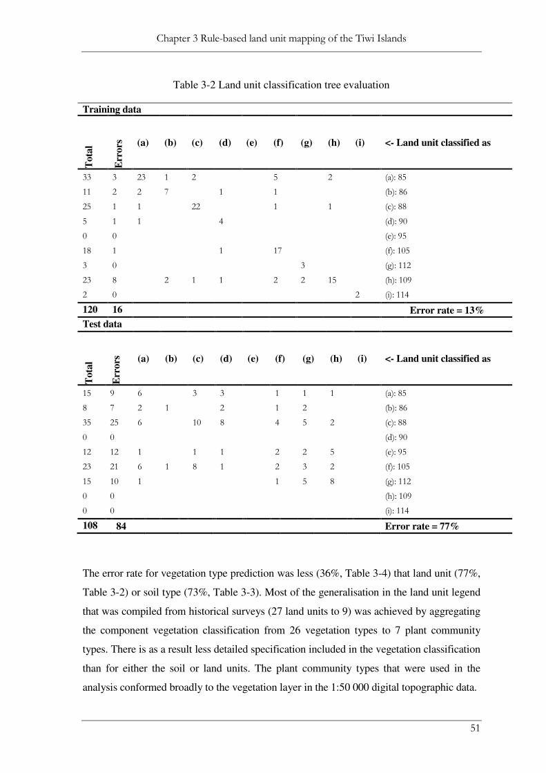
Chapter 3 Rule-based land unit mapping of the Tiwi Islands
51
Table 3-2 Land unit classification tree evaluation
Training data
Tota
l
Err
ors
(a) (b) (c) (d) (e) (f) (g) (h) (i) <- Land unit classified as
33 3 23 1 2 5 2 (a): 85
11 2 2 7 1 1 (b): 86
25 1 1 22 1 1 (c): 88
5 1 1 4 (d): 90
0 0 (e): 95
18 1 1 17 (f): 105
3 0 3 (g): 112
23 8 2 1 1 2 2 15 (h): 109
2 0 2 (i): 114
120 16 Error rate = 13%
Test data
Tota
l
Err
ors
(a) (b) (c) (d) (e) (f) (g) (h) (i) <- Land unit classified as
15 9 6 3 3 1 1 1 (a): 85
8 7 2 1 2 1 2 (b): 86
35 25 6 10 8 4 5 2 (c): 88
0 0 (d): 90
12 12 1 1 1 2 2 5 (e): 95
23 21 6 1 8 1 2 3 2 (f): 105
15 10 1 1 5 8 (g): 112
0 0 (h): 109
0 0 (i): 114
108 84 Error rate = 77%
The error rate for vegetation type prediction was less (36%, Table 3-4) that land unit (77%,
Table 3-2) or soil type (73%, Table 3-3). Most of the generalisation in the land unit legend
that was compiled from historical surveys (27 land units to 9) was achieved by aggregating
the component vegetation classification from 26 vegetation types to 7 plant community
types. There is as a result less detailed specification included in the vegetation classification
than for either the soil or land units. The plant community types that were used in the
analysis conformed broadly to the vegetation layer in the 1:50 000 digital topographic data.

Chapter 3 Rule-based land unit mapping of the Tiwi Islands
52
Table 3-3 Soil classification tree evaluation
Training data T
ota
l
Err
ors
(a) (b) (c) (d) (e) (f) (g) (h) (i) (j)
<- Soil family
classified as
34 11 22 9 1 1 1 (a): Hotham
44 9 4 35 1 4 (b): Berrimah
9 1 1 8 (c): Mirrikau
9 3 1 6 2 (d): Ramil
2 2 2 (e): Irgil
6 3 2 3 1 (f): Kiluppa
3 0 3 (g): Wangitti
2 2 1 1 (h): Rinnamatta
10 5 1 2 1 1 5 (i): Marrakai
1 1 1 (j): Koolpinyah
120 37 32 50 13 13 0 5 7 0 9 0 Error rate = 31%
Test data
Tota
l
Err
ors
(a) (b) (c) (d) (e) (f) (g) (h) (i) (j) <- Soil family
classified as
11 7 3 3 4 1 (a): Hotham
28 10 7 14 1 2 2 2 (b): Berrimah
13 12 4 1 1 0 7 (c): Mirrikau
14 13 5 3 1 1 1 3 (d): Ramil
2 2 1 1 0 (e): Irgil
14 13 6 4 1 1 1 0 1 (f): Kiluppa
1 0 1 (g): Wangitti
1 2 1 0 (h): Rinnamatta
13 9 6 2 1 4 (i): Marrakai
11 11 6 4 1 (j): Koolpinyah
108 79 13 32 8 4 0 1 6 0 4 0 Error rate = 73%
3.4 Discussion and conclusions
Land unit surveys have a tendency to over–specify land unit classes in relation to the
field survey data sets, even in low relief landscapes with fairly monotonous lithology such
as the Tiwi Islands. This has also been identified as a map quality issue in Australian land
resources mapping (McKenzie and Austin, 1993). Consequently, the expectations of end

Chapter 3 Rule-based land unit mapping of the Tiwi Islands
53
users of land unit mapping need to be attuned to the need for further field survey work to
meet specific information requirements.
The traditional land resources survey method produces a knowledge base that is expressed
in soil map legends and can be formalized in terms of sets of mapping rules based on
distributed environmental attributes (Bui, 2004). DTA produces sets of rules that are
analogous to traditional survey methods. However, with this digital soil mapping technique
it is possible to upgrade the mapping, or knowledge base, in a way that is consistent with
current soil and land survey practice as more field survey data become available. In the
Tiwi Islands mapping, additional surveys were environmentally stratified according to
landform pattern and landform element classes, in the same way as traditional soil
resources surveys are designed (Speight, 2009). The main innovation is in substituting
digital terrain analysis for physiographic interpretation from aerial photography.
Plate 3-1 Soil mapping – reddish colours indicating
Oxisols, grey Ultisols and blues Aquic soils
A general finding was that there is less error in the test and training data sets for vegetation
class predictions than for soil and land unit class predictions (Tables 3-2 and 3-3). Plant
communities tend to compensate for edaphic variation by changing their topographic
positions (Guisan and Zimmermann, 2000) and the responses to landscape variation may

Chapter 3 Rule-based land unit mapping of the Tiwi Islands
54
not be consistent with soil patterns. Reducing the vegetation classes from 26 to 7 was made
to rationalise land unit definitions. The general classification of vegetation communities
that was produced is clearly more amenable to prediction from the data that was available.
Some factor information could be improved as new environmental layers for geology based
on gamma-radiometric mapping have become available that reveals the distribution of
bedrock and regolith materials with sufficient detail to show variations at local scales
(Minty et al., 2009).
Table 3-4 Vegetation classification tree evaluation
Training data
Tota
l
Err
ors
(a) (b) (c) (d) (e) (f) (g) (h) (i) (j) <- Vegetation classified
as
92 2 90 2 (a): Eucalypt forest
7 6 2 1 1 3 (b): Melaleuca forest
6 2 2 4 (c): Mangrove forest
10 0 10 (d): Vine Forest
0 0 (e): Sparse woodland
4 0 4 (f): Grassland/sedge
1 1 1 (g): Coastal woodland
120 11 Error rate = 9%
Test data
Tota
l
Err
ors
(a) (b) (c) (d) (e) (f) (g) <- Vegetation classified
as
81 14 67 3 11 (a): Eucalypt forest
14 14 11 1 2 (b): Melaleuca forest
0 0 (c): Mangrove forest
9 7 7 2 (d): Vine Forest
3 3 2 1 (e): Sparse woodland
0 0 (f): Grassland/sedge
1 1 1 (g): Beaches/cheniers
108 39 Error rate = 36%
The simplification of the land unit classification that were needed to apply digital soil
mapping techniques to land unit mapping on the Tiwi Islands demonstrate the level of
inference that can be drawn reliably from land unit survey information. The mapping

Chapter 3 Rule-based land unit mapping of the Tiwi Islands
55
legend derived in this study is more general than the land unit classification obtained from
legacy soil surveys. It is likely that land unit map legends contain inaccuracies, often
associated with duplication, derived from mapping by different soil surveyors and tend to
overstate the environmental inferences that can be made, particularly in regard to vegetation
communities. However, a digital soil mapping approach to updating legacy soil survey data
and mapping would appear to have many advantages in the digital age not the least being
the ability to integrate new knowledge with the knowledge accumulated over the years. Our
test data set comprised site information extracted from legacy soil surveys conducted 20 to
30 years ago. The inaccurate location of legacy soil survey data is an issue when this data is
used to develop and test predictive models (Bui and Moran, 2001).
Issues associated with the inaccuracy of legacy land resource survey data and the
complexity of the land unit model limit its value and reliability for selecting natural
analogue areas to guide landscape restoration and conservation strategies. Consequently,
test area surveys are needed to check and develop environmental inferences that will
support reliable interpolation of soil and vegetation properties across the landscape.
Significant landform effects on vegetation communities were identified using a DSM
methodology based on the land unit concept. However, a high level of survey support will
be needed to predict species distributions. Focussing this survey support in landscapes that
are analogous to the restoration goals of mine rehabilitation rather than distributing them to
assess the broad range of regional environmental variation will simplify the ecological
modelling and improve the reliability of the predictions that are made.

Chapter 4 Natural analogue landform selection for planning mine landscape restoration
56
Chapter 4 Natural analogue landform selection for planning
mine landscape restoration
4.1 Introduction
It was recognised from the regional mapping of land units using digital soil mapping
methods reported in Chapter 3 that focussing environmental surveys on analogous areas of
natural landscapes was likely to produce more reliable statistical predictions of vegetation
pattern. Also, it was recognised that the reliability of the inferences that could be made
from regional ecological mapping such as land units was low, due to the lack of sufficient
survey support for a complex conceptual model. Consequently, staged ecosystem survey
approach that has a stronger basis in ecological theory is now developed. A landscape
classification and natural analogue selection method is developed in this chapter that
applies extent and grain size concepts used in habitat classification in landscape ecology.
This approach relates the extent of mining disturbance and the grain size of hillslope
environmental processes to the type and range of habitats that open cast mining impacts
upon at a particular site. The approach is staged from broad reconnaissance in this chapter
to detailed survey (reported in Chapter 6) to focus survey efforts in order to support
accurate inference.
Environmental investigations at the Ranger case study site are presented in Chapters 4 to7
that support an ecological design approach using natural analogues. This approach could be
extended where a restoration approach to rehabilitation is required. In Chapter 5, the soil
profile in a constructed waste rock landform at Ranger uranium mine is characterised and
water and solute balance investigated and compared with published information on natural
soils.
In Chapter 6, an ecological landform design based on the geomorphic properties of a
natural analogue area is independently assessed using deterministic modelling methods and
a detailed, second stage investigation of soil and plant community patterns that leads
directly on from Chapter 4 is reported on. In Chapter 7, species distribution modelling that
used survey support from Chapter 6 is undertaken so as to test whether mine landform
design could be expected to create similar vegetation patterns found in an analogous natural
landscape. Because of the low level of predictability of vegetation and soils reported in

Chapter 4 Natural analogue landform selection for planning mine landscape restoration
57
Chapter 3 from land unit mapping, the work reported in Chapter 7 was the key development
from this thesis.
In the current chapter, natural analogue areas and environmental correlation of landform
with plant community and soil morphological properties is investigated using digital terrain
analysis and patch analysis methods that reflect environmental grain size and extent
properties of habitats in hill slope environments.
4.1.1 Landform scale
Scale has been described as the fundamental conceptual problem in ecology (Levin,
1992) that is reflected in the spatial dependence of vegetation pattern on landform (Miller et
al., 2007). Since digital raster analysis methods were introduced to landscape ecology, scale
has been conceptualised in terms of grain size and extent (Wu et al., 2002) rather than as a
map scale. A similar conceptual change, albeit with different terminology, is repeated in
other landscape sciences such as digital soil mapping (McBratney et al., 2003). This has
happened in response to high resolution raster, environmental data becoming available over
extensive areas as an improvement on thematic information.
However, in spite of this conceptual development in gridded landscape models, analogue or
reference ecosystem selection for mine rehabilitation is typically qualitative and subjective,
and based on thematic land unit mapping (Zonneveld, 1989) or other regional
environmental information (Hobbs and McIntyre, 2005). For example, natural analogue
selection to set mine rehabilitation objectives at the Ranger case study site initially focussed
on similarities in surface geology (Uren, 1992), geochemical factors (Riley and Rich, 1998)
and rocky habitats represented in land units with regional context (Brennan, 2005). This has
happened although local gradients in plant available water supply and soil drainage are
known to affect short range ecosystem variation (Williams et al., 1996) and would be better
represented in terms of grain size and extent properties of analogous natural landscapes.
In the context of Ranger mine, the environmental range that was sampled by Brennan
(2005) to identify analogues was limited to well drained eucalypt woodland habitats 100
hectares in extent on land units with rocky substrates. The environmental properties
associated with landform extent and relief at vegetation plot survey sites was overlooked
and hill slope environmental gradients in water supply and drainage were not considered in

Chapter 4 Natural analogue landform selection for planning mine landscape restoration
58
the survey design. The very detailed vegetation information produced from plot studies
without a detailed landscape context comparable to the mine landscape may lead to
unforeseeable outcomes in the rehabilitation design.
For instance, where an analogue selection approach based on land units was used at the
now closed Nabarlek uranium mine (150 kilometres to the north east of Ranger mine),
Klessa (2000) reported that native woodland failed to establish on the reconstructed
landscape. Unexpected ecological outcomes such as this are common on mined land
restoration projects (Nicolau, 2003) and may be due to neglecting the extent of mining
impacts in selecting the analogue area(s) and the grain size of hillslope environmental
processes that affect the vegetation patterns to be restored, and failing to design landforms
that accommodate this pattern.
The landscape model used affects the analogue selection process (Fischer et al., 2004;
Lindenmayer et al., 2008). However, the topographic detail relevant to site restorations has
been difficult to identify and factor into environmental restoration plans for a number of
reasons outlined in Hobbs & McIntyre (2005). Landscape environmental variation is
complex and crosses different dimensions that affect species distributions at local and broad
regional landform scales. For instance, hillslope curvature affects concentrated water flow
and distribution locally, while aspect and landform relief influence the radiant energy
environment affecting vegetation growth and potential energy driving geomorphic
processes over broader landform patterns, lands systems and bioregions (Franklin et al.,
2000; Gessler et al., 2000; Nelson et al., 2007; Urban et al., 2002; Wilson and Gallant,
2000b). To address this landscape scale is considered in standard methods of soil and
landscape assessment (Speight, 2009) and the local and regional factors in landscape
classification and habitat variation are reflected in hierarchical habitat classification systems
(Cushman and McGarigal, 2002; Mackey et al., 2008).
The natural ecosystem variation that results from landform variation is typically patchy,
combining both discrete and continuous variation resulting from endogenous ecological
processes as well as environmental heterogeneity related to landscape. The stochastic
nature of ecological processes requires a statistical approach to survey design, comprising
replication and environmental stratification across local landscapes. However, landscape
characteristics need to be determined in an ecologically meaningful and methodologically
sound way (Wagner and Fortin, 2005). To accomplish this, landscape ecologists have used

Chapter 4 Natural analogue landform selection for planning mine landscape restoration
59
different patch based metrics depending on landscape scale (extent and grain size) to
develop environmental associations to characterise habitat variation (Neel et al., 2004; Wu
and Levin, 1997; Wu et al., 2002).
A key concern in applying patch analysis methods is that the grain size and patch metrics
need to link with underlying hillslope environmental processes (Bowman and Minchin,
1987; Ludwig et al., 2002; Ludwig et al., 2000b; Wu and Archer, 2005) to be of practical
value for landscape restoration (Li and Wu, 2004). Also a level, or levels, of regionalisation
is required to address questions of landscape utility, i.e. in the case of this study what part,
or parts, of the natural landscape reflect the habitat type range that applies to restoring a
mined, waste rock landscape. However, it must be recognised that landscapes function in an
environmentally integrated way. Consequently, the analogue selection process that is most
likely to reflect this will include an interconnected range of habitats found in natural
hillslope environments that match the extent of mined landscape restoration task.
When conceptual ecological mapping frameworks (such as land units) are used as a
regionalising factor to landform in habitat analysis, hillslope topographic details are
overlooked and subjective and sometimes arbitrary boundaries are introduced (see Chapter
3). Alternatively, grid overlays have been used to represent the extent of landscape utility
with respect to foraging animal range (Rempel and Kaufmann) or soil property mapping
(Hollingsworth et al., 2007; McBratney et al., 2003) in quantitative landscape analysis.
Selecting a particular landform extent, as well as environmentally appropriate patch
metrics, is a key consideration in answering the ecological questions being asked in mine
restoration based on natural analogues. It is proposed that localised mining activity is
analogous to foraging animal range in the way that the extent of landscape utility is defined.
However, the habitat concepts being applied in mined land restoration may not be linked to
the range of any particular species, but rather the distribution of plant communities in local
hillslope environments. These habitat concepts need to be defined and this is done in the
next section.
4.1.2 Habitat concepts
There are two meanings of the term habitat in use, one that is organism specific and
another that is land based and it is important to distinguish how the term is being applied

Chapter 4 Natural analogue landform selection for planning mine landscape restoration
60
(Miller and Hobbs, 2007). In the first instance, habitat is typically defined as an area
containing the particular combination of resources and environmental conditions that are
required by individuals of a given species or group of species to carry out life processes.
Odum (1971) provided an alternative, broader definition of habitat as “The area or
environment where an organism or ecological community normally lives or occurs”. In this
case, an ecosystem is a community of interacting organisms and their physical environment
while habitat refers specifically to the physical environment in which they live.
An extension of the second usage of the term, the concept of habitat types, provides a
general framework for understanding the ecological processes that operate at landscape
scales. The composition of habitat types in a landscape and the physiognomic or spatial
arrangement of those habitats are the two essential features that are required in an
ecological description of any landscape (Dunning et al., 1992). Since digital terrain analysis
underpins current methods in species and plant community distribution modelling (Austin,
2007; Guisan and Zimmermann, 2000), extending the concept of habitat type in this thesis
to include patterns derived from digital terrain variables that represent environmental
variation across landscapes (Wilson and Gallant, 2000a) is reasonable. Using digital terrain
analysis to develop habitat type classifications advances the procedure of identifying
natural analogue landscapes to represent restoration objectives for mine landscape
reconstruction.
4.1.3 Patch analysis
Multivariate classification of fine grained environmental surfaces is the basis of
habitat type classification used in this approach (McGarigal et al., 2009). The approach
termed patch analysis averages variation in habitat type, described by cluster analysis of
continuous fine grained environmental surfaces, into patches and derives ecologically
meaningful patch metrics, according to the extent of a dependant variable, or object of
interest across an extensive landscape (Wagner and Fortin, 2005). In this method, a
hexagonal grid, or tessellation, is overlaid on the patch mosaic to represent the extent of
local landscape structure that can be related to habitat use (Rempel and Kaufmann). Other
grid shapes could be used, but hexagonal grids stack well, project onto the spherical surface
of the earth with minimal distortion and are more representative of average conditions
(because the perimeter is more or less equidistant from the centre) than rectangular grids for
spatial averaging (Sahr et al., 2003). The extent of the grid elements used varies with the

Chapter 4 Natural analogue landform selection for planning mine landscape restoration
61
context of the study in relation to species foraging range (Rempel and Kushneriuk, 2003;
Rempel and Kaufmann, 2003).
Patch metrics based on vegetation pattern and land use have been criticised as lacking
ecological significance, which limits the understanding of underlying environmental
process that can be derived (Li and Wu, 2004; Miller and Hobbs, 2007). Surface metrics
derived from terrain and image analysis have been used that address this shortcoming,
(Cushman and McGarigal, 2004a; Cushman and McGarigal, 2004b; McGarigal et al., 2009;
Neel et al., 2004). Patch area metrics have been found to be relatively robust across a range
of landscape structural extents (McGarigal et al., 2009; Wagner and Fortin, 2005). Also,
landscape metrics related to class area may have strong relationships with species dispersal
(Neel et al., 2004). Although, the links between the landscape gradients being measured by
surface metrics and ecological consequences still need to be understood.
Similarity (or dissimilarity) may be assessed at sequentially higher levels in the patch
analysis process — starting with classification of continuous fine grained environmental
surface properties into a range of habitat types, followed by classifying landscape structural
extents on the basis of contained habitat types so as to select natural landscapes analogous
to an object of interest. Ecological surveys designed to assess the environmental factors that
drive landscape environmental variation, represented by surface metrics, are required (Li
and Wu, 2004). However, landscapes of similar extent with similar patch metrics are
assumed to represent a similar habitat range. Consequently, the analogue selection process
leads into reconnaissance ecological surveys that are structured around inferred
environmental variations and are aimed at confirming the selection process and identifying
environmental processes that affect species composition and community variation in
analogue areas. This approach assumes that the habitat type classification can be related to
measured ecosystem variation and that the direct impact from a mined landscape is
analogous to foraging animal range.
4.1.4 Environmental Factors
In hillslope situations, where physiography exerts strong control over vegetation
patterns (Bowman and Minchin, 1987; Ludwig et al., 2002; Wu and Archer, 2005) terrain
properties connected to environmental processes such as water balance, drainage,
sedimentation and erosion are correlated with plant community variation (Franklin et al.,

Chapter 4 Natural analogue landform selection for planning mine landscape restoration
62
2000). Fire frequency and intensity can also determine suitable conditions for a given
species in seasonally dry savannah woodlands such as those that occur across much of
northern Australia (Williams et al., 2003b). Although Bowman & Minchin (1987)
concluded that the edaphically determined vegetation controlled fire regime rather than the
converse. This study identified strong topographic control between Melaleuca communities
from those dominated by eucalypts in a very gently undulating landscape with subtle
topographic variation.
Bowman & Minchin (1987) used indirect gradient analysis of vegetation survey data in the
Australian monsoon tropics near Darwin to reveal strong relationships between the
vegetation pattern and edaphic variables that reflected two aspects of the moisture regime –
water availability during the dry season and the degree of inundation during the wet season.
Moisture availability was determined by topographic position, through its relationship with
soil texture and water table depth. Poor drainage during the wet season separated Melaleuca
communities in drainage lines from eucalypt communities on slopes, while shrubby and
grassy open forests were differentiated by the intensity of the winter drought. There is an
alternative point of view that fire can affect vegetation pattern rather than the reverse
(Fensham, 1990; Gill et al., 2003; Grant and Loneragan, 2001). Also gradient analysis
methods that directly constrain the ordination by environmental factors (Leps and Smilauer,
2003) are popular for environmental analysis of species distribution, although underlying
assumptions of linearity are not robust and can artificially distort the results (McCune and
Grace, 2002).
4.1.5 Statistical methods
4.1.5.1 Cluster analysis
Cluster analysis for groupings of similar sample sites identifies discontinuity and can
be used in combination with gradient analysis and network analysis (connecting groups
based on similarity) for comprehensive multivariate evaluation of ecological pattern in field
survey data (Margules and Austin, 1991). Clustering can imply a simple partitioning (a set
of non-overlapping clusters) or a more complex hierarchical pattern. A general form of
hierarchical clustering based on the Bray Curtis measure of dissimilarity (Bray and Curtis,
1957) and UPGMA (group average) called flexible UPGMA allows the variation of a
dilation parameter, β, that influences success in cluster recovery. Flexible UPGMA with a

Chapter 4 Natural analogue landform selection for planning mine landscape restoration
63
small negative β value has been shown to recover cluster structure well from noisy data
(Belbin and McDonald, 1993).
While some hierarchical algorithms may be robust for ecological survey data, all of these
methods are limited in terms of the number of sites that can be analysed, because a matrix
of all pair-wise dissimilarities among sites must be calculated. For large data sets (1000
objects or more) such as remote sensing, extensive digital elevation models and their
derivatives, non-hierarchical methods that search directly for a fixed number of groups,
e.g., k-means clustering are more effective and reliable (Belbin, 1987; Bui and Moran,
2001).
4.1.5.2 Gradient analysis
Several environmental factors can determine species and plant community
distribution in any particular situation and either direct (Austin, 2002a; Oksanen and
Minchin, 2002) or indirect (Margules and Austin, 1991; McCune and Grace, 2002) gradient
analysis methods have been developed to investigate relationships in community and
landscape ecology. With direct gradient analysis sample sites are positioned according to
measured environmental factors to elucidate species response to specific gradients of
interest. Univariate response can be measured by regression (Austin, 2002b; Guisan et al.,
1999) and multivariate responses are measured in terms of the statistical significance of
ordination scores and correlations between axis scores and external environmental variables
(Margules and Austin, 1991; McCune and Grace, 2002).
In contrast, indirect gradient analysis that ordinates survey sites according to covariance
and association among species, with the benefit of reflecting the environmental space the
way the biotic community interprets, is widely accepted (Austin, 1987; Austin, 2002a;
Belbin, 1995; Ben Wu and Archer, 2005; Bio et al., 1998; Bowman and Minchin, 1987;
Mackey et al., 2008; Margules et al., 1987; McCune and Grace, 2002; Minchin, 1987a).
Ordination is first performed on just the community data, and then secondarily related to
the ordination of the environmental variables, followed by an independent assessment of
the importance of the environmental variables. Although quantitative relationships are not
produced, indirect gradient analysis using nonmetric multidimensional scaling (NMS) it
considered to accurately represent species space (Margules and Austin, 1991; McCune and
Grace, 2002).

Chapter 4 Natural analogue landform selection for planning mine landscape restoration
64
Indirect analysis of multivariate gradients is, however, difficult to visualise. Consequently,
hybrid methods (Leps and Smilauer, 2003) particularly canonical correspondence analysis
(CCA) that constrain the ordination in species space by correlations with environmental
variables are popular in community ecology (Grant and Loneragan, 2001; Rayfield et al.,
2005; ter Braak, 1996; Zhu et al., 2005).
The assumptions of simple linear relationships between species and environmental space
used in hybrid analysis are often questioned and the methods themselves can create
distortion (McCune and Grace, 2002; Minchin, 1987a). While detrending can be used to
remove distortions (Enright et al., 1994) this may also confound clear interpretation
(McCune and Grace, 2002). Hybrid ordination methods also ignore community structure
that is unrelated to the environmental variables and the results can be unreliable as a
consequence (Guisan et al., 1999). In general, direct gradient methods provide better
species specific-models; hybrid methods such as CCA may provide a broader overview of
multiple species, while indirect gradient analysis best represents species space and
subjectively assesses environmental gradients.
Gradient analysis is highly sensitive to survey design (Austin and Meyers, 1996).
Stratification that takes into account both the grain and extent of the pattern of patches
across the landscape and replicated sampling of environmental factors across the habitat
range of interest is needed to support statistical evaluation of environmental variation
(Cushman and McGarigal, 2002; Fischer et al., 2004; McKenzie and Ryan, 1999;
McKenzie et al., 1989).
4.1.6 The way forward from thematic landscape models
Understanding the landscape characteristics that underlie environmental processes
and determine environmental heterogeneity in natural landscapes underlies a more reasoned
approach to analogue area selection to for landscape restoration (Holl et al., 2003; Palik et
al., 2000). Although, species responses depend on the resolution and choice of response
variables and patch arrangement in the landscape (Ben Wu and Archer, 2005; Ludwig et
al., 1999) quantitative landscape models have been used to map soils (McBratney et al.,
2003), habitats (Austin, 2002b; Li et al., 2001) and species distribution (Guisan and
Zimmermann, 2000) that rely on continuous, high resolution environmental information
from remote sensing and digital terrain analysis (Wilson and Gallant, 2000b).

Chapter 4 Natural analogue landform selection for planning mine landscape restoration
65
4.2 Methods
A first stage, reconnaissance investigation is presented designed to identify
appropriate natural analogue landforms for planning landscape reconstruction at the Ranger
uranium mine case study site in the Top End of the Northern Territory of Australia.
4.2.1 Study area location
Ranger uranium mine is located in the Ranger project area (79 km2 in area) at 12⁰ 41’
Lat 132⁰ 55’ Long, 250 km east of Darwin and is surrounded by 19 803 km2 of coastal
plain and escarpment conserved in the world heritage listed Kakadu National Park (Figure
4-1).
Figure 4-1 Ranger location map
The climate of the region is monsoonal with a wet season from October to March during
which 95% of the annual rainfall occurs (mean 1700 mm), followed by a prolonged dry
season characterised by little or no rainfall (Heerdegen and Cook, 1999; Taylor and
Tulloch, 1985). Low plant available water supply and impaired soil drainage affect short
TIWI ISLANDS

Chapter 4 Natural analogue landform selection for planning mine landscape restoration
66
range ecosystem variation in a local climatic environment that is marked by seasonal
drought (Williams et al., 1996). The climate is similar to that of the Tiwi Islands described
in Chapter 3.
4.2.2 Vegetation
Savanna communities dominate the region. A discontinuous tree canopy layer with a
seasonal understorey of grasses characterises these communities. Eucalyptus miniata-E.
tetrodonta savannas form the framework within which other important vegetation
communities occur (Schodde et al., 1987). Savanna vegetation type is associated with
lateritic peneplains in undulating terrain where soils are typically deep, well-drained and
light textured. In the vicinity of Ranger Mine, this vegetation occurs over deeply weathered
metamorphic rocks and granite. On rises and upper slopes where soils are shallow and more
gravely, rusty-barked bloodwood (Eucalyptus bleeseri) is a major component. On gentle
slopes in the undulating lowlands over metamorphic rocks, granite and dolerite Eucalyptus
tectifica- E. latifolia savannas are the most widespread vegetation, except on very poorly
drained soils. Soils tend to be heavier textured loams and clay loams, shallower, and less
well drained.
4.2.3 Geology, geomorphology and soils
Kombolgie Formation Sandstone, Nanambu Formation gneisses and schists, and
Cahill Formation schists and quartzites crop out in the area (Needham, 1988). Extensive
coastal alluvial sediments are associated with a backswamp of the East Alligator River (the
Magela Plain). Freshwater sediments are associated with the tributary creeks, and sandy,
colluvial sheet wash fans radiate out from the base of the Arnhem Plateau and the Jabiluka
outlier in the north, east and south and cover low lying parts of the landscape. A lateritised
surface, known as the Koolpinyah Surface (Nott, 1994b) extends to the south of the
Jabiluka outlier of the Arnhem Plateau, and relatively small areas of ferruginized sandstone
occur on the outlier itself.
The Koolpinyah Surface can have a thick, weathered (ferruginized) zone that may extend
up to 60 m into the bedrock below the present soil cover. The unit includes gradational and
uniform Red and Yellow Earth soils on lateritic remnants with minor skeletal and
gradational Yellow Earths on slopes. Dissected, lateritised remnants of the lowland

Chapter 4 Natural analogue landform selection for planning mine landscape restoration
67
Koolpinyah Surface are also associated with scree slopes and outwash fans at the base of
the plateau outlier between 20 and 50m elevation (Hollingsworth et al., 1998).
The Supervising Scientist for the Alligator Rivers Region (Wasson, 1992) undertook
detailed geomorphic and pedological study of the Magela Creek Plain. They described acid
peats overlying clays of estuarine origin and interpreted the evolution of the plain and the
implications for contaminant management. White and Gigliotti (1982) and (Morley et al.,
1985) measured detailed chemistry on profiles of selected soils in association with the
Pancontinental proposal to mine the Jabiluka deposit. Their work also concentrated on the
Magela floodplain. Hollingsworth et.al. (1998) described components of the Swift Creek
alluvial system, and the Jabiluka system comprising the sheet wash fans from the plateau
surfaces, and the peneplain of lateritised schists, or Koolpinyah system that extends south
of the Jabiluka outlier, and the Magela Plain to the Ranger mine.
The soils in the Swift Creek and Jabiluka land systems are sandy throughout and show
minimal soil profile development apart from organic matter accumulation at the surface and
iron oxide accumulation in the sub-soil. The soils in the Koolpinyah land system have
profiles with clay accumulation in the sub-soil and typically have an iron cemented
(ferricrete) pan within 1 meter of the surface. The soils in the Magela land system are very
poorly drained and have sulfidic and sulfuric horizons, commonly within 1 meter of the
surface. The limited soil development is related to the siliceous nature of the parent
materials, the lack of weatherable minerals and the erosivity and high drainage flux
associated with the monsoonal rainfall environment (Duggan, 1991). Although it seems
incongruous, the residual soils have formed in a stable environment over a long period of
time (Nanson et al., 1993; Nott, 1994a).
4.2.4 Fire environment
Fire frequency and intensity is also an important environmental factor in these
ecosystems. Eucalypt dominant woodlands tend to be fire resistant (Andersen et al., 2005)
and frequent, high intensity fires produced by late dry season burning reduce biodiversity,
principally in the understorey and groundcover (Bowman et al., 2003; Russell-Smith et al.,
2003; Williams et al., 2003b). Consequently, differences in fire frequency and intensity
between analogue areas and surrounding national park could produce differences in
vegetation pattern that may be unrelated to topographic variation.

Chapter 4 Natural analogue landform selection for planning mine landscape restoration
68
4.2.5 Terrain analysis
The process was used to construct the DEM of the Ranger site and it’s surrounds was
the same as that used for the Tiwi Islands study (described in Section 3.2.2), except that
more accurate contour data (1 metre versus 5 metre) derived from corrected and contoured
laser altimetry data was available from mapping contractors for ERA Ranger mine. This
potentially improved the resolution of the DEM. A DEM extending northwards from the
Ranger site in a swath approximately 6 kilometres wide and 25 kilometres long was created
using ANUDEM 4.6 software (Hutchinson, 1997). Drainage lines mapped at 1:50 000 were
overlaid with contour lines and spot heights from orthophoto mapping at 1: 10 000
standards of accuracy and a splined elevation surface was generated by ANUDEM that
respected the natural surface drainage. The model included a topographically reconstructed
mine landform that respected the original relief and drainage density. The model was
checked for sinks, which were filled.
The higher resolution contour data and increased spatial resolution for the Ranger elevation
data lead to a preliminary assessment of the optimum DEM resolution to be used in the
analysis that follows. The effects of DEM resolution on the ability to make environmental
inference has been studied elsewhere (Gallant and Hutchinson, 1997; McBratney, 2004;
Wilson and Gallant, 2000b). The optimum resolution may vary with landscape relief to
some extent (McKenzie et al., 2000) and can be estimated from the minimum root mean
square (RMS) slope of all DEM points associated with the elevation data (Kienzle, 2004;
Wilson and Gallant, 2000b). RMS analysis for the Ranger data indicated that the optimum
DEM resolution was 10 metres in high relief plateau and escarpment landscapes and was
something greater than this (approximately 30 metres) for low relief. The 20 metre grid
resolution used to fit the terrain model was within the capability of the source data and able
to resolve hill slope variation in low relief landscapes.
The suite of terrain attributes shown in Table 4-1 were generated using TAPESG (Gallant
and Wilson, 1996) and have been hypothesised to be important determinants of the
distribution of plants and ecological communities (Parker and Bendix, 1996). Newer terrain
analysis software such as SAGA (Cimmery, 2007) provide graphical user interfaces, can
generate wider range of secondary terrain attributes and are able to process laser altimetry
(Lidar) data rather than contours (Ryan and Boyd, 2002). New terrain attributes have been

Chapter 4 Natural analogue landform selection for planning mine landscape restoration
69
specifically developed that describe flow patterns more accurately in low relief landscapes
(Gallant and Dowling, 2003) but these are not critical for representing flow in hillslopes.
In TAPESG, different options are provided for determining flow direction (D8, Rho8, or
Frho8), flow accumulation (D8, multiple flow paths, and Costa-Cabral' method), and slope
gradient (D8 or finite difference). Other related programs in the bundle include DYNWET
for calculating wetness index, EROS for soil loss and erosion and deposition potential,
SRAD for estimating solar radiation. In summary, TAPESG is still one of the more
versatile software packages available in terms of flow routing algorithms that can be used
on different surfaces and the environmental attributes that are generated in hillslope
environments are still valid (Nelson et al., 2007).
Table 4-1 Environmental attributes calculated by
terrain analysis from DEM data
Attribute Module Environmental interpretation
primary terrain attribute
elevation TAPESG climate, vegetation, potential energy, geomorphology
slope TAPESG overland and subsurface flow velocity and runoff rate, precipitation, vegetation, geomorphology
aspect TAPESG solar insolation, flora and fauna distribution, evapotranspiration
profile curvature TAPESG flow acceleration, erosion/deposition rate, geomorphology
plan curvature TAPESG converging/diverging flow, soil water content, soil characteristics
secondary terrain attribute
erosion–deposition index EROS erosion/sedimentation rate, nutrient supply, landscape function, vegetation, soil depth and texture
static topographic wetness index
DYNWETG plant available water, soil drainage status, vegetation, groundwater dependant ecosystems
4.2.6 Habitat class mapping
Continuous surfaces for slope, elevation, wetness index, and erosion/deposition index
at 20 metre grid resolution were output from terrain analysis (422 892 grid cells in each
environmental layer) representing the grain of environmental variation across an extensive
lowland and highland landscape (Figure 4-2).

Chapter 4 Natural analogue landform selection for planning mine landscape restoration
70
Figure 4-2 Continuous environmental surfaces for
elevation, slope, soil wetness index,
erosion/deposition index, and derived (k-means
clustering) habiat type map with a hexagon (500 ha)
outlining the Ranger landform
Habitat was classified from this data, using a non-hierarchical, k-means, classification
strategy (Mackey et al., 2008; Mackey et al., 1988) in the PATN 3.03 (Belbin, 2008)
software package to produce more than the desired number of classes. Hierarchical
classification routines in PATN were used to evaluate structure in the initial classification
to identify a desirable number of classes from the shape of the dendrogram before
rerunning the non-hierarchical classification (Belbin, 1991). 11 habitat classes were
classified from the environmental layers. The functions within PATN facilitate multivariate
pattern analysis on large and complex data sets. The parameter values for the classifications
are provided in Table 4-2.

Chapter 4 Natural analogue landform selection for planning mine landscape restoration
71
Table 4-2 Environmental attributes and codes used in
the analysis
No. Attribute Attribute codes
Land surface
1 drainage 1=very poor 2=poor 3=imperfect 4=moderate 5=well 6=rapid
2 runoff 0=none 1=very slow 2=slow 3=moderate 4=rapid 5=very rapid
3 permeability 1=very slow 2=slow 3=moderate 4=high
Substrate
4 substrate depth in metres
5 substrate lithology 1=colluvium(CL) 2=ferricrete(FC) 3=schist(ST) 4=sandstone(SA) 5=alluvium(AL)
Soil classification
6 soil order 1=kandosol(KA) 2=hydrosol(HY) 3=rudosol(RU) 4=tenosol(TE)
7 soil sub-order 1=red(AA) 2=orthic(DS) 3=oxyaquic(DT) 4=brown(AB) 5=leptic(CY) 6=yellow(AC) 7=redoxic(ED) 8=stratic(ER)
8 soil great group 1=regolithic(GF) 2=petroferric(EA) 3=mesotrophic(AG) 4=paralithic(DU) 5=dystrophic(AF)
9 soil sub-group 1=basic(AR) 2=ferric(BU) 3=melanic(DK) 4=rendic(EF) 5=haplic(CD) 6=mottled(DQ) 7=bleached(AT)
Soil morphology
10 A horizon thickness 1=thin(A) 2=medium(B) 3=thick(C)
11 surface gravel 1=none(E) 2=slight(F) 3=common(G) 4=moderate(H) 5=very(I)
12 A horizon texture 1=sandy(K) 2=loamy(L) 3=clay loamy(M)
13 B horizon texture 1=sandy(K) 2=loamy(L) 3=clay loamy(M) 4=clayey(O)
14 soil depth 1=very shallow(T) 2=shallow(U) 3=moderate(V) 4=deep(W)
Digital terrain analysis
15 aspect TAPESG, octant coded for slopes greater than 0.5%
16 wetness TAPESG (DYNWETG) dynamic wetness index
17 elevation tapesg (m)
18 slope tapesg (%)
19 erosion TAPESG (EROS) erosion/sedimentation index
20 easting E location of site from SW origin
21 northing N location of site from SW origin
Landform description
22 landform element 1=crest(HCR) 2=drainage depression(DDE) 3=swamp(SWP) 4=slope(HSL) 5=talus(TAL) 6=valley flat(VLF) 7=bench(BEN)
23 slope morphology 1=crest(C) 2=lower slope(L) 3=flat(F) 4=vale(V) 5=upper slope(U) 6=mid slope(M)
PATN calculates a measure of the dissimilarity in the association metric used between a set
of objects based on the values for the variables used to describe the objects. Each
environmental variable was standardised, prior to classification, dividing by its range to
remove bias due to differences in the units of measurement. In this case, the objects were

Chapter 4 Natural analogue landform selection for planning mine landscape restoration
72
20 metre grid cells and the variables were several environmental variables. The output was
a habitat class map. Following field ecological surveys this could be considered to be a
habitat type map.
4.2.7 Natural analogue selection
A hexagonal mesh of 500-hectare polygons was overlaid on the habitat class map to
constrain the analogue landform selection process to natural landforms similar in extent to
the mine landform. One element of the mesh covered the Ranger mine landscape. The
habitat class map was intersected with the 500-hectare mesh and the areas of each habitat
class were summed in each mesh element. The landscape classification derived in this way
identified two landforms of the same extent as the mine landform and with a similar range
and proportion of habitat classes. These landforms were assumed to support similar levels
of ecosystem variation, which was assessed from subsequent field surveys described below
in Section 4.2.9.
4.2.8 Fire environment
Fire frequency and intensity in the analogue areas was compared with surrounding
areas of Kakadu National Park using publicly available, time series remote sensing. The
monthly fire scar maps, derived from MODIS satellite data for the Northern Territory from
January 1996 until July 2003 were acquired from the West Australian Department of Land
Information web site (Marsden, 2003). Fires prior to 1 August were classified as less
intense early fires and those after were categorized as more intense late fires. The fire
frequencies were normalised (years in 10) for early and late fires and an analogue area was
compared to similar habitats elsewhere in KNP (Schodde et al., 1987) to check whether
there were likely to be obvious differences in the fire environment between the analogue
area and other areas surrounding the mine.
4.2.9 Environmental survey design
A stratified survey design (Austin and Heyligers, 1989) with three replicate transects
at two toposequence sites in the each of two selected analogue landforms was applied to
describe soil, land surface and plant species presence-absence according to standard
reconnaissance survey methods (McDonald et al., 2009). Sites were selected along each

Chapter 4 Natural analogue landform selection for planning mine landscape restoration
73
toposequence to sample different mapped habitat classes from the crests to the valley flats.
The patterns in the field survey data were initially evaluated using indirect gradient
methods including multivariate classification, ordination and network analysis methods in
the PATN program.
4.2.10 Indirect gradient analysis of environmental variation
4.2.10.1 Classification
Two site data sets were input separately into PATN: (i) vegetation data as defined by
species presence–absence and, (ii) environmental data derived from the terrain analysis and
derived from soil and landscape descriptions taken during the field survey work. Species
presence–absence was scored for each site in a species data matrix of 1’s and 0’s. Species
that occurred only once were masked out of the analysis. Species that are this sparsely
distributed do not add information to a classification process based on pair-wise
dissimilarity measures and classification improves if they are removed. Initially there were
123 species recorded at 35 sites. Masking out species with single occurrences left 79
species with multiple occurrences. The environmental data set contained a mixture of ratio,
ordinal and nominal observations recorded at each site. The nominal and ordinal variables
were coded to integer values to facilitate numerical analysis. The environmental attributes
and coding used are shown in Table 4-2.
The association measure used was the Czekanowski coefficient. This is the presence-
absence equivalent of the measure attributed to Bray and Curtis (1957). The values range
from ‘0’ meaning identical to ‘1’ inferring that the two sites have no species in common.
This measure has been shown to be appropriate for the type of data being analysed here
(Faith et al., 1987). Hierarchical polythetic clustering based on the association measure
(Czekanowski) was used to fuse sites into groups. The unweighted pair-group method
(UPGMA) from Sneath and Sokal (1973) was used to provide a best fit between the input
association measures and what is termed the ultrametric distances implied from the
dendrogram. The flexible version of the UPGMA implemented in PATN incorporates a
variable (β=-0.1) that allows for a slight dilation in the fusion strategy, adjusting for
insensitivity that occurs when sites have few of no species in common.
The site group definitions were copied from the species to the environmental dataset and
Significant environmental differences between site groups were identified by the Kruskal-

Chapter 4 Natural analogue landform selection for planning mine landscape restoration
74
Wallis statistic. The sites and then species were clustered to define site by species
groupings in a two–way table. The data file for species presence–absence data file was
edited to mask out singular species occurrences that did not add information to the pairwise
association measure.
The species data matrix was then transposed to classify the species on the basis of where
they occurred. This revealed species that tended to occur together. A two-step association
measure was applied to account for the lack of ‘duality’ in the site as by species
classification process (Belbin, 1991). The site and species classifications were then imposed
on the data matrix to create a two-way table. This imposed the dendrogram ordering, with
the defined groups, back on the raw data and was a useful check of the results of the
classification process.
4.2.10.2 Ordination
Overall trends are more identifiable using ordination than classification. Non-metric
multi-dimensional scaling was used because it is well suited to data that are non-normal, or
are on arbitrary, discontinuous scales and is the method of choice for ecological community
data (Margules and Austin, 1991; McCune and Grace, 2002; Minchin, 1987a). Ordination
placed the sites in a reduced number of dimensions that reflected the Bray Curtis measures
of association. Multiple linear regressions of the environmental variables on the ordination
vectors were performed to determine vectors of maximum environmental correlation with
ordination space. Visual confirmation of the relationships between groups and
environmental vectors was obtained by presenting the data in a minimum spanning tree of
site classes in ordination space.
4.3 Results
4.3.1 Terrain modelling and habitat class maps
The terrain modelling results, and the combined habitat class map that was derived
from these results was depicted in Figure 4-2. Typically slopes were less than 3% and the
erosion/deposition index varied between -1 and 1 typical of low relief, water shedding
surfaces. However, upland plateau landform dominated the landscape to the north and west
of the study area. The upland plateau was associated with the Arnhem Land escarpment and
contrasted with the lowland peneplain on which the mine site was located. A three
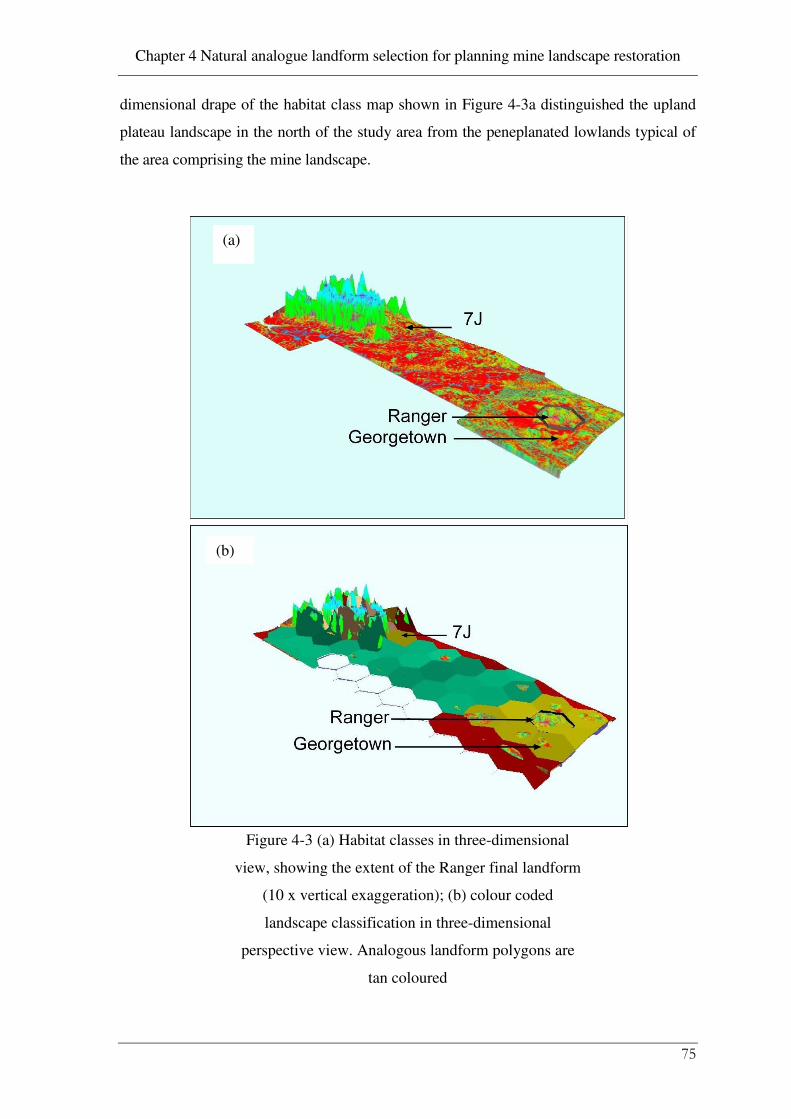
Chapter 4 Natural analogue landform selection for planning mine landscape restoration
75
dimensional drape of the habitat class map shown in Figure 4-3a distinguished the upland
plateau landscape in the north of the study area from the peneplanated lowlands typical of
the area comprising the mine landscape.
Figure 4-3 (a) Habitat classes in three-dimensional
view, showing the extent of the Ranger final landform
(10 x vertical exaggeration); (b) colour coded
landscape classification in three-dimensional
perspective view. Analogous landform polygons are
tan coloured
(a)
(b)

Chapter 4 Natural analogue landform selection for planning mine landscape restoration
76
Significant differences occurred between median values of slope, elevation, wetness index
and erosion–deposition index between habitat classes. These are highlighted using box
plots of the range in significantly different (according to the Kruskal Wallace statistic)
terrain parameters for each habitat class in Figure 4-4.
The interpreted geomorphic process in each of the 11 habitat classes is given in Table 4-3.
Habitat classes 2, 3 and 10 were likely to be aggraded by sediment according to their
geomorphic attributes and erosion-deposition index. Habitat classes 1, 3, 8 and 11 were
likely to be wetter than other classes according to wetness index ranges.
Figure 4-4 Box plots showing the range in
environmental attributes for each habitat class
mapped. The inner quartile range shown by the boxes
highlights differences between the classes. Whiskers
indicate outer quartile range and points indicate
outliers.

Chapter 4 Natural analogue landform selection for planning mine landscape restoration
77
Table 4-3 Geomorphic description of habitat classes
Habita
t class
Slope
(%)
Geomorphic
environment
Land surface Wetness Landform
Description
1 low erosional lowland not inundated crests
2 gentle erosional lowland not inundated slopes
3 gentle
depositional lowland seasonally inundated
lower slope
4 gentle
erosional lowland not inundated shoulder slopes
5 steep erosional upland not inundated plateau escarpment
6 gentle
erosional lowland not inundated crests of low hills
7 steep erosional upland not inundated upper slopes
8 gentle
depositional lowland regularly inundated
drainage depressions
9 gentle to moderate
deposition and erosion are active
upland not inundated plateau surface
10 moderate to steep
depositional upland seasonal inundation
talus slopes and fans
11 moderate to steep erosional lowland and upland
inundated stream channels
4.3.2 Landscape classification natural analogue selection
The landscape classification was made based on the relative areas of each of the 11
habitat classes described above in each 500 hectare tile (64 covering the study area)
representing landscape structure. The dendrogram of the association matrix was assessed
visually and a cut was made into 9 groups (Figure 4-5a). The part of the dendrogram
showing linkages between the Ranger mine and similar landscape areas (Cluster 3) is
shown in Figure 4-5b. The Ranger mine are and landscapes of the same extent that were
similar to it in terms of habitat mix comprised the most extensive part of the overall
landscape (27 observations/hexagons). The choice of two prospective natural analogue
areas – Georgetown and 7J, as indicated on Figure 4-3b, reflects their close linkage to the
habitat properties of the Ranger mine area, based on the association measures that are used.
Other reasons were that the 7J area is physically remote from the Ranger site while the
Georgetown area is adjacent to the mine. Both areas have similar underlying parent
materials to the mine according to regional geological mapping (Needham, 1988). The
depiction of the proposed analogue areas on Figure 4-3a, b indicates their geographic
separation by approximately 10 kilometres.

Chapter 4 Natural analogue landform selection for planning mine landscape restoration
78
Figure 4-5 (a) Dendrogram showing linkages between
500 hectare hexagons representing landscape
structural extent (observations, horizontal cut line for
6 groups); (b) detailed dendrogram for Cluster 3
comprising the Ranger mine and similar areas
(a)
(b)
Cluster 3
Ran
ger
7 J
Geo
rgeto
wn

Chapter 4 Natural analogue landform selection for planning mine landscape restoration
79
Geographic separation was identified as an issue that determined some properties of these
areas in the subsequent environmental survey and analysis. Both of the selected landforms
were observed to be rocky rises, similar in scale and topography to the Ranger site. The 7J
analogue area abutted a high relief plateau 10-km to the north of the study area while the
Georgetown area was immediately adjacent to Ranger mine. The most extensive landscape
component in the selected landform patterns were the gently sloping erosional surfaces.
4.3.3 Fire environment
There were three habitat types that were defined by regional (KNP) habitat mapping
(Schodde et al., 1987), represented in the analogue landforms (Figure 4-6). Brighter hues in
Figure 4-6 indicated less frequent fires. Less frequent early dry season fires and more
frequent late dry season fires occurred in the analogue area than in the surrounding parts of
KNP.
The total dry season fire frequency was similar in the analogue area and selected habitats in
KNP. In summary, late dry season fires were more frequent in the analogue area than in
similar habitats in KNP, but the fire environments and habitat range were similar.
4.3.4 Vegetation patterns
123 species were recorded in the environmental survey. After masking out singular
observations (90% annuals) that occurred once, the remaining 79 species were used in the
analysis (Table 4-4). Multivariate classification distinguished nine site groups shown in
Table 4-5. Site groups 2 and 5 were represented by one site each on sandy outwash fans in
the 7J analogue area. Classifying the transposed sites by species table produced six groups
of species that commonly coexisted shown in Table 4-5.
The common or extensive plant community types such as species group 1 occurred in all
site groups except site group 2 (Table 4-5). Other species groups were well-represented in
particular environments. Matrix cells with notable species-site associations in Table 4-5 are
highlighted by shading. Species group 3 was well represented in site group 1, which were
all on sandy substrates. Species group 4 was well represented on the wet sandy substrates in
site group 2. Species group 6 was well represented in poorly drained areas with ferruginous
subsoil horizons in site groups 4 and 6. Apart from their absence in site group 1 (sandy
substrates) the pattern of site distributions for species groups 2 and 5 was indistinct, i.e.

Chapter 4 Natural analogue landform selection for planning mine landscape restoration
80
they were poorly defined by the habitat variation that was sampled. Otherwise dense
localised patterns of species and site groups in the two-way table indicated that the analysis
was robust.
Figure 4-6 KNP habitat mapping units (Schodde,
1987) represented in analogue areas with fire
frequency mapping showing detail in the Georgetown
area
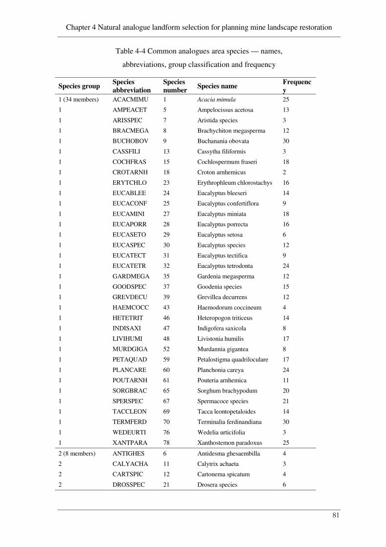
Chapter 4 Natural analogue landform selection for planning mine landscape restoration
81
Table 4-4 Common analogues area species — names,
abbreviations, group classification and frequency
Species group Species
abbreviation
Species
number Species name
Frequenc
y
1 (34 members) ACACMIMU 1 Acacia mimula 25
1 AMPEACET 5 Ampelocissus acetosa 13
1 ARISSPEC 7 Aristida species 3
1 BRACMEGA 8 Brachychiton megasperma 12
1 BUCHOBOV 9 Buchanania obovata 30
1 CASSFILI 13 Cassytha filiformis 3
1 COCHFRAS 15 Cochlospermum fraseri 18
1 CROTARNH 18 Croton arnhemicus 2
1 ERYTCHLO 23 Erythrophleum chlorostachys 16
1 EUCABLEE 24 Eucalyptus bleeseri 14
1 EUCACONF 25 Eucalyptus confertiflora 9
1 EUCAMINI 27 Eucalyptus miniata 18
1 EUCAPORR 28 Eucalyptus porrecta 16
1 EUCASETO 29 Eucalyptus setosa 6
1 EUCASPEC 30 Eucalyptus species 12
1 EUCATECT 31 Eucalyptus tectifica 9
1 EUCATETR 32 Eucalyptus tetrodonta 24
1 GARDMEGA 35 Gardenia megasperma 12
1 GOODSPEC 37 Goodenia species 15
1 GREVDECU 39 Grevillea decurrens 12
1 HAEMCOCC 43 Haemodorum coccineum 4
1 HETETRIT 46 Heteropogon triticeus 14
1 INDISAXI 47 Indigofera saxicola 8
1 LIVIHUMI 48 Livistonia humilis 17
1 MURDGIGA 52 Murdannia gigantea 8
1 PETAQUAD 59 Petalostigma quadriloculare 17
1 PLANCARE 60 Planchonia careya 24
1 POUTARNH 61 Pouteria arnhemica 11
1 SORGBRAC 65 Sorghum brachypodum 20
1 SPERSPEC 67 Spermacoce species 21
1 TACCLEON 69 Tacca leontopetaloides 14
1 TERMFERD 70 Terminalia ferdinandiana 30
1 WEDEURTI 76 Wedelia urticifolia 3
1 XANTPARA 78 Xanthostemon paradoxus 25
2 (8 members) ANTIGHES 6 Antidesma ghesaembilla 4
2 CALYACHA 11 Calytrix achaeta 3
2 CARTSPIC 12 Cartonema spicatum 4
2 DROSSPEC 21 Drosera species 6

Chapter 4 Natural analogue landform selection for planning mine landscape restoration
82
Table 4-4 continued
Species group Species
abbreviation
Species
number Species name
Frequenc
y
2 ERIAOBTU 22 Eriachne obtusa 3
2 GRASSPEC 38 Grass species 5
2 PAVEBROW 56 Pavetta brownie 2
2 SOWEALLI 66 Sowerbaea alliaceae 6
3 (15 members) ACACONCI 2 Acacia oncinocarpa 4
3 ALLOSEMI 4 Alloteropsis semialata 2
3 COLERETI 16 Coleospermum reticulatum 5
3 COMMENSI 17 Commelina ensifolia 5
3 DENHOBSC 19 Denhamia obscura 4
3 DOLIFILI 20 Dolichandrone filiformis 9
3 GARDSCHW 36 Gardenia schwarzii 4
3 GREVGOOD 40 Grevillea goodii 3
3 HETECONT 45 Heteropogon contortus 3
3 OWENSPEC 53 Owenia species 4
3 PACHJUNC 54 Pachynema junceum 5
3 PERSFALC 57 Persoonia falcata 6
3 PETAPUBE 58 Petalostigma pubescens 13
3 SETAAPIC 64 Setaria apiculata 3
3 THECPUNI 73 Thecanthes punicea 8
4 (6 members) CLEOSPEC 14 Cleome species 2
4 GARDRESI 34 Gardenia resinosa 2
4 GREVPTER 42 Grevillea pteridifolia 2
4 LOPHLACT 49 Lophostemon lactifluus 2
4 MELANERV 50 Melaleuca nervosa 3
4 VERTCUNN 75 Verticordia cunninghamii 2
5 (6 members) ACACSPEC 3 Acacia species 7
5 CALYEXST 10 Calytrix exstipulata 7
5 EUCALATI 26 Eucalyptus latifolia 6
5 RHYNLONG 62 Rhynchospora longisetis 2
5 SYZYEUCA 68 Syzygium eucalyptoides 2
5 TERMPTER 72 Terminalia pterocarya 8
6 (10 members) FICUOPPO 33 Ficus opposita 2
6 GREVMIMO 41 Grevillea mimosoides 3
6 HAKEARBO 44 Hakea arborescens 4
6 MELAVIRI 51 Melaleuca viridifolia 8
6 PANDSPIR 55 Pandanus spiralis 5
6 SEDGSPEC 63 Sedge species 3
6 TERMGRAN 71 Terminalia grandiflora 2
6 UTRISPEC 74 Utricularia species 2
6 WRIGSALI 77 Wrightia saligna 11
6 XYRISPEC 79 Xyris species 2

Chapter 4 Natural analogue landform selection for planning mine landscape restoration
83
Table 4-5 Two-way table of sites groups (rows) verses
vegetation species groups (columns) with notable
species-site associations highlighted by shading
AAABBCCCEEEEEEEEEGGGHHILMPPPSSTTWX|ACCDEGPS|AACCDDGGHOPPPST|CGGLMV|ACERST|FGHMPSTUWX
CMRRUAORRUUUUUUUUAORAENIUELOOPAEEA|NAARRRAO|CLOOEOAREWAEEEH|LAROEE|CAUHYE|IRAEAEETRY
APIACSCOYCCCCCCCCROEETDVRTAURECRDN|TLROIAVW|ALLMNLRETECRTTE|EREPLR|ALCYZR|CEKLNDRRIR
CESCHSHTTAAAAAAAADDVMEIIDANTGRCMET|IYTSASEE|COEMHIDVENHSAAC|ODVHAT|CYANYM|UVEADGMIGI
MASMOFFACBCMPSSTTMSDCTSHGQCABSLFUP|GASSOSBA|OSREOFSGSSJFPAP|SRPLNC|SELLEP|OMAVSSGSSS
ICPEBIRRHLOIOEPEEEPEORAUIUARRPEERA|HCPPBPRL|NEENBICOPPUAUPU|PETAEU|PXAOUT|PIRIPPRPAP
MEEGOLANLENNRTECTGECCIXMGARNAEORTR|EHIETEOL|CMTSSLHOEENLBIN|ESECRN|ESTNCE|PMBRIEAELE
UTCAVISHOEFIROCTRACUCTIIADEHCCNDIA|SACCUCWI|IIIICIWDCCCCECI|CIRTVN|CTIGAR|OOOIRCNCIC
| | | | |
B1 * ** * * * * ** * | | * * *| | |
B3 * *** * * * * * | | * ** ** * | | |
C1 * * * * * * * * ** *** | |* ****** ******| | |
C2 * * * * * * * * ** *** | |* ****** ******| | |
C3 * * * * * * * * ** *** | |* ****** ******| | |
C4 * * * * * * * | |* * * | *| | *
----------------------------------+--------+---------------+------+------+----------
B4 | * *| * |******| |
----------------------------------+--------+---------------+------+------+----------
D1 ** * *** ** * ** **** ** *| | * * | | |*
D2 ** ** ** * ** ** * * * ***** *| * | * *| | | *
D3 ** * * * ** ** * * * ***** *| | | | |
E1 * * * ** * **** ** ** * * *| | | |** *|
E2 * * * * * **** ** ** * * *| | | |* *|
F1 ** ** * ** ** * * * **** *| | * *| |* |
F3 ** ** * * *** ** * * ** *| | * * | | * | *
F4 * * * * ** * * ** ***** * *| * | | * |* * |
K2 ** * *** * * ********* *| * * | *| |* *|
K3 * * **** * ** **** * *| | * | | |
----------------------------------+--------+---------------+------+------+----------
D4 * * * * * * |* * *| * * | | | ***** *
K4 * * ** * *| *| | | *| *** **
L4 * * * * * | * *| | * | * | ** **
----------------------------------+--------+---------------+------+------+----------
E3 * * *** * * ** * ** * | *******| * | * | * *| **
----------------------------------+--------+---------------+------+------+----------
H1 ** * * * * *** * * ** *** * *| | * | | |
H2 * * ** * * * * * * * *|* * | * | | |
H3 ** * * ** * ** * * * * * * * *|* | | | |
M2 ** * ******** **** ** ** * *| * | * | | | *
M3 ** ** * * * ****** * ** ******| * ** | * * | | * |
----------------------------------+--------+---------------+------+------+----------
K1 * * * * ***** ** * ** * *| | *| | * |
L1 * * *** * ** ** * *| | * * | | | *
L2 * * * ** *** * * *| * | * | | ** | *
M1 * ***** **** * *** ***** * ***| | * | | * | *
----------------------------------+--------+---------------+------+------+----------
E4 * * * * * * ** *** *|* ** * *| * | | *| *
K5 ** * ** * * * ** * *| * | * | * |******| *
L3 * ** * * * * * *** *| * | * | * |* * **| **
----------------------------------+--------+---------------+------+------+----------
L5 * ** * * ** **** *| | * |* | * |***** * **
M4 * **** * * ** * * * ** * ****| | * | | | ** *

Chapter 4 Natural analogue landform selection for planning mine landscape restoration
84
Best fit attributes and corresponding correlations (according to vector lengths) were
identified by displaying the fit of environmental factors to NMDS plots for axis 2 versus
axis 1 (Figure 4-7a) and axis 3 versus axis 1 (Figure 4-7b). Soil texture (A and B horizon),
drainage class, soil great group, soil permeability class, substrate depth, runoff rate and
wetness index were all highly correlated with species ordination space.
A- and B-horizon texture, drainage status and runoff rate were prominent in the left-bottom
quadrant of the ordination plot (Figure 4-7a). Groups 3 and 6 were the most extensive site
groups in this quadrant and occurred on slopes and crests of low rise landforms where the
soils were well drained. Wetness index and substrate depth, acted in the top-right quadrant
of the ordination plot (Figure 4-7b). Groups 1, 2, 4 and 8 sites populated this quadrant.
Group 2 is a single site group occurring in the swamps located on deep colluvial sands.
However, group 1 sites were better drained on the same sandy colluvium. Group 4 occurred
on the lower slopes of the low rises formed in deeply weathered mica schist, while group 8
occurred on alluvial valley flats. Groups 7 and 5 sites populated the north east quadrant of
the ordination. No strong environmental associations were evident in this quadrant. Group 9
occurred in the south west quadrant and occurred in level or very gently sloping landform
elements with a cemented ferricrete layer between 0.5 and 1.0 m depth. Ferricrete substrate
occurred at both group 9 and group 5 sites.
The minimum spanning tree network (Figure 4-8) showed site group linkages and the
directions of strong environmental gradients in the ordination space, highlighting similar
ecological groups and environmental driving factors. The minimum spanning tree
accurately represents the distance between close objects, a slightly different focus to
ordination. Group 2 was very distinct, although quite similar to group 5. Both these groups
occurred in poorly drained locations on sandy colluvial substrate. Group 5 occurred on a
transition between sandy colluvium and rocky rises with lateritised substrate rocks of mica
schist. Consequently, group 5 was linked to group 3, which was the most extensive
environment type surveyed.
Group 3 occurred in both analogue survey areas on slopes and crests of rises formed in
weathered mica schist. Group 3 was linked to groups 6, 1 and 8 (Figure 4-8). The linkage
was closest with group 6, predominantly on gentle to moderately rocky slopes. Group 1 is
distinctly different from the rest of the groups and occurred on crests and slopes on the
sandy colluvial landforms.

Chapter 4 Natural analogue landform selection for planning mine landscape restoration
85
Figure 4-7 Scattergrams from ordination showing
strongly correlated environmental variables
Axis 1
Axis
2
a)
wetness
A texture
drainage
runoff
perm
eabi
litygreat g
roup
-
-
-
-
-
.
.. .
. .
.
. .
.
.
+
+.
..
+
+ +
. ..
... . +
...
...
.. ..
.. .
....
-
-
-
-
-
--
- - - - - - - -
---- -- - -
A textur
e
B texture
dra
inage
depth
gre
at goup
perm
eabili
ty
wetness
Axis
3
Axis 1
-
-
-
-
-
-
-
-
-
-
-
-
-
..
.
.
. ......
...
.
.
.
.
..
.
.
++
++
+
+ ..
.
..
.
....
....
.
..
-
- - - - -
---------
--- -
b)
0
-1
-5 -4 -3 -2 -1 1 2 3
-
-5 -4 -3 -2 -1 1 2 3
1
2
3
4
0
-1
1
2
3
4
-2
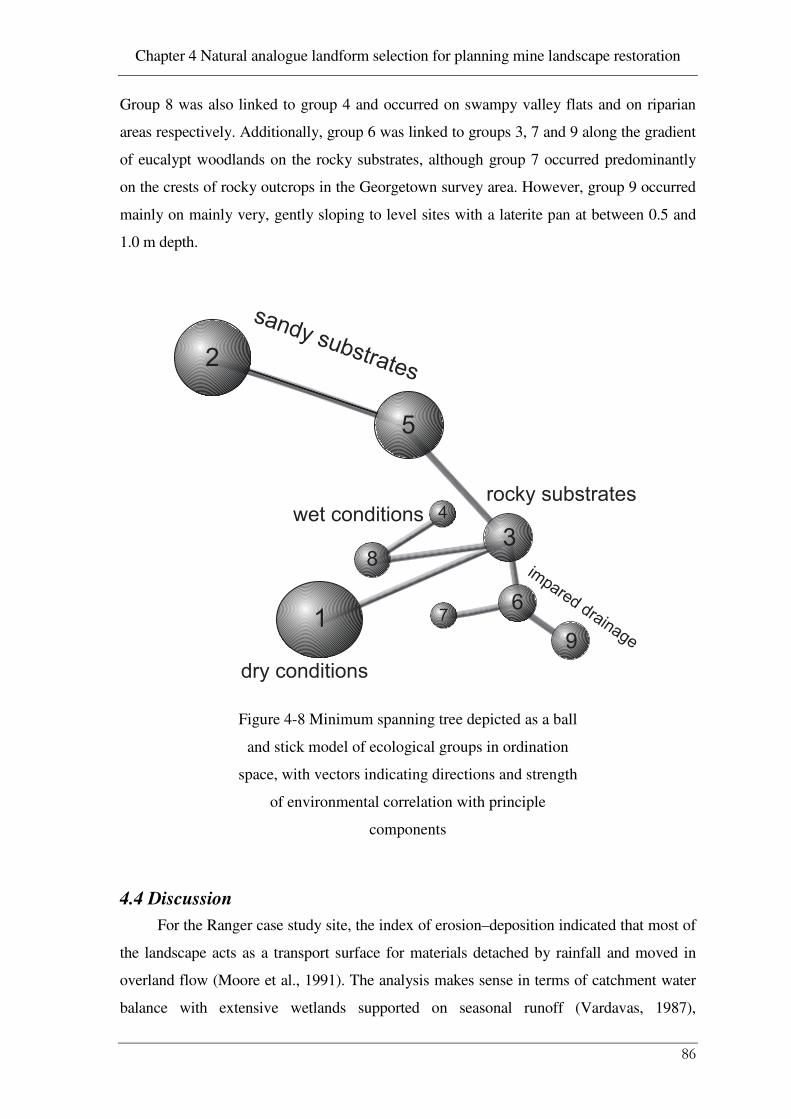
Chapter 4 Natural analogue landform selection for planning mine landscape restoration
86
Group 8 was also linked to group 4 and occurred on swampy valley flats and on riparian
areas respectively. Additionally, group 6 was linked to groups 3, 7 and 9 along the gradient
of eucalypt woodlands on the rocky substrates, although group 7 occurred predominantly
on the crests of rocky outcrops in the Georgetown survey area. However, group 9 occurred
mainly on mainly very, gently sloping to level sites with a laterite pan at between 0.5 and
1.0 m depth.
Figure 4-8 Minimum spanning tree depicted as a ball
and stick model of ecological groups in ordination
space, with vectors indicating directions and strength
of environmental correlation with principle
components
4.4 Discussion
For the Ranger case study site, the index of erosion–deposition indicated that most of
the landscape acts as a transport surface for materials detached by rainfall and moved in
overland flow (Moore et al., 1991). The analysis makes sense in terms of catchment water
balance with extensive wetlands supported on seasonal runoff (Vardavas, 1987),
2
5
1
83
4
76
9
rocky substrates
sandy substrates
impared drainage
wet conditions
dry conditions

Chapter 4 Natural analogue landform selection for planning mine landscape restoration
87
environmental processes related to the energy environment (Odum and Odum, 2003) and
local variation in landscape ecology (Ludwig et al., 2002).
Environmental processes that underlie ecological pattern are resolved and then aggregated
to a scale that represents the system being studied. The high resolution landscape metrics
that reflect the hill slope hydrology are robustly correlated with landscape function and the
ability to retain material resources. This is supported elsewhere for perennial vegetation in
Australian rangelands and savanna woodlands (Bastin et al., 2002; Bowman and Minchin,
1987). Applied at a high enough resolution to identify environmental range in hill slope
environments and aggregated to describe ecological systems that are in context with the
mine landscape, these methods could be adapted from a broad regional context to
quantifying local environmental variation specific to mining disturbance and selecting
natural analogues for mine restoration planning.
Analogue areas comprised broad variation in habitat class across hill slope environments.
Environmental properties of sites in habitat classes in selected analogue areas varied in
plant community (used to represent ecosystem type), soil drainage and substrate properties
such as texture and gravel content that directly relate to plant available water storage. This
corroborates the intuitive understanding of vegetation patterns in the savanna woodland
environments in KNP (Wilson et al., 1991) related to water and sediment balance (Bowman
et al., 1993).
All of the extensive savanna communities in the larger KNP area (Schodde et al., 1987)
were represented in the reconnaissance survey. Out of the nine site groups (used to
represent ecosystem type) five were broadly categorised as lowland eucalypt woodland and
mixed eucalypt woodland and a sixth (group 4) as myrtle-pandanus savanna (sensu
Schodde 1987). Three groups (groups 1, 2 and 5) were associated with sandy sheet wash
fans emanating from the base of the upland Arnhem Plateau in the 7J analogue area, while
all of the measured environmental range on weathered schist substrates was present in the
Georgetown analogue area. This gives confidence in focussing environmental surveys on
the Georgetown analogue area. The environmental range represented in this analogue
landform was wider than that sampled in previous analogue surveys for Ranger mine over a
wider geographic extent (Brennan, 2005).

Chapter 4 Natural analogue landform selection for planning mine landscape restoration
88
These findings emphasise the importance of including hill slope variation in selecting an
analogue landform for the purpose of providing environmental support for restoring mined
landscapes. The approach addresses the requirement expressed by Bell (1997) that
landscape structures need to be introduced as a central theme in environmental variation to
aid restoration efforts. Also required is the appropriate landscape context that is essential
for selecting natural analogues. The importance of a landscape context has been recognised
before (Duque et al., 1998; Ehrenfeld and Toth, 1997; Hobbs and McIntyre, 2005; Holl et
al., 2003; Huttl and Bradshaw, 2001). However, this study presents more robust analogue
selection methods that were focussed on the mined landscape rather than regional
conservation objectives, which would have confounded rather than completed the picture of
restoration objectives.
The concept of similar areas, identified from multivariate analysis of continuous
environmental data derived from a DEM (Bryan, 2003; McGarigal and Marks, 1995) is
adapted to specify the environmental pattern within at the scale of the mine landscape that
needs to be restored. Understanding environmental pattern and scale is a central problem
where basic ecology needs to be applied to describe phenomena that vary in space and time
(Levin, 1992). In landscape restoration, the function of the larger landscape assemblage
depends on patchiness in the distribution of resources in smaller units (Ludwig et al., 2004).
Landscape assembly and linkage is intrinsic to the methodology used here. The range of
analogue ecosystems was physically linked in a functioning landscape and based on
detailed (20-m grid) environmental data. For instance the wetland and riparian sites were
successfully discriminated from the woodlands on rock outcrops and mixed eucalypt
woodland sites that were contiguous on hill slopes. These hill slope environmental features
have been overlooked in past analogue studies focussed on a regional context (Brennan,
2005; Grant, 2006; Hobbs and McIntyre, 2005). Although these features are known to be
important (Bowman et al., 1993; Russell-Smith, 1995; Wardell-Johnson and Horwitz,
1996) they have been difficult to assess (Dirnbock et al., 2002).
The current study also identified environmental gradients that are more important in a
regional rather than local landscape context. For instance an analogue area, 10 kilometres
away from the mine, had more extensive areas of vegetation communities in which
Corymbia bleeserii is common. This woodland species is associated with relatively drier
conditions (Williams et al., 1996) and its prevalence may be due to local rain shadow

Chapter 4 Natural analogue landform selection for planning mine landscape restoration
89
effects from surrounding plateau areas. Consequently, analogue data from areas that are
remote from the mine site may introduce some complexities into the analysis and
quantitative assessment based on environmental correlation and regression (Austin, 2002b).
Care must be taken to exclude extraneous environmental gradients if regional
environmental surveys are used to select analogues.
The frequent late dry season fires in the analogue and surrounding areas of KNP are a
common feature of savanna woodland environments in the Top End dominated by eucalypt
woodland (Andersen et al., 2005). The management of fire frequency and intensity is likely
to have profound effect on the survival of eucalypt species early in the revegetation
program (Williams et al., 1999). However, similarities in fire environment in analogue
areas and surrounding areas of KNP (based on the review of fire frequency in Section 4.3.2)
influence similar mature woodland communities in terms of species distribution and
community structure.
The selected natural analogues areas are representatives of lowland environmental variation
in context with the mine landform — without sacrificing environmental variation found
over an extensive area. This is a very useful result considering the fact that previous
analogue surveys were far more extensive and covered a narrower environmental range
(Humphrey et al., 2005). Appreciating the connectedness of landscape is important, as
upland landforms can exert strong localised influences on soils, vegetation and probably
local climate in surrounding lowlands. The approach developed here preserved the context
of hill slope environmental variation at the mine scale and carefully excluded extraneous
escarpment environments that fringe upland plateau landscapes.
Inappropriate analogues or reference sites associated with broader landscape diversity can
be identified and avoided by ensuring that the reconnaissance environmental survey
sampled each habitat class to provide a clear focus on the environmental range relevant to
the mine area. Generalising environmental variation using regional topographic references
as proposed by Hobbs & McIntyre (2005) would not have provided an accurate context for
selecting analogue areas in this instance.

Chapter 4 Natural analogue landform selection for planning mine landscape restoration
90
4.5 Conclusions and further studies
4.5.1 Conclusions
Terrain analysis resolved patterns of hill slope environmental variation in low relief
landscapes and identified extensive water shedding surfaces and wetter run-on areas.
However, variation in substrate properties was linked to colluvial geomorphic processes in
the surrounding landscapes. Using a landform extent and patch metrics based on the
component areas of different habitat types answered the key question of what part, or parts
of the natural landscape were appropriate to the mine restoration task. In this respect,
localised mining activity was considered to be analogous to foraging animal range in the
way that the extent of landscape utility is defined. The habitat concepts being applied were
not linked to the range of any particular species, but rather the distribution of plant
communities in local hillslope environments – particularly between Melaleuca and eucalypt
woodland communities and discriminated environmental gradients in eucalypt woodland
type that were related to soil and landscape properties reflecting plant water supply and
drainage.
Landscape factors related to water and sediment distribution, drainage and plant available
water supply in the soil exerted significant control over the distribution of vegetation types
in seasonally dry savannah environments. Individual natural analogue landforms may
contain a wide range of ecosystem types, representing the environmental range that occurs
on hill slopes over a much more extensive area. Selecting analogues using a combination of
terrain analysis, multivariate landscape classification and structured environmental surveys
is a practical approach. This set of procedures is structured to provide a clear context with
the scale of a mine landform and high resolution of environmental variation based on a
DEM. Other environmental data sets can be introduced as required. For instance substrate
mineralogy may be an issue that can be described from remotely sensed passive radiometric
data (Bollhöfer et al., 2008). Multi-spectral and hyper-spectral data also have potential
application for assessing a range of environmental factors (Ustin et al., 2004).
However, understanding factors that affect ecosystem variation within hill slope
environments appears from this analysis to be more appropriate for planning landscape
restorations following opencast mining than geochemical, geological or regional context.
Landscape structural extent and environmental grain size are useful concepts – replacing
concepts of map scale and resolution from thematic mapping – to develop landscape
Chapter 4 Natural analogue landform selection for planning mine landscape restoration
91
models for environmental analysis and analogue selection. Also, the proximity of natural
analogue areas to the site to be restored may be a consideration in cases where there are
steep rainfall and climatic gradients.
A quantitative approach to selecting analogue landforms is developed here that is based on
multivariate statistical and patch analysis methods that are in general use in conservation
and landscape ecology. Continuous surfaces of high resolution environmental information
and multivariate analysis methods that were developed to select reserve habitats for
conservation and landscape planning (Bryan, 2003; Margules and Austin, 1991; McGarigal
and Marks, 1995; Rempel and Kushneriuk, 2003; Rempel and Kaufmann, 2003) could be
applied to select natural analogue areas. Although, the resolution and scale used to describe
ecosystem variation will be critical to adapting the method to the particular application
(Levin, 1992).
4.5.2 Further studies
The analogue selection approach and multivariate analysis of environmental pattern
presented in this chapter leads to more detailed survey supporting direct gradient analysis in
Chapter 7. However, the natural analogue approach that has been presented implies that the
properties of the surface cover in the mine landform can resemble the range of natural soils.
Restoring comparable plant available water storage and drainage conditions in the
constructed mine soils appears to be particularly important to demonstrate support for
comparable woodland communities. The implications of land surface and landform cover
construction on soil properties and revegetation response are investigated in Chapter 5.

Chapter 5 Mine landform cover design and environmental evaluation
92
Chapter 5 Mine landform cover design and environmental
evaluation
5.1 Introduction
5.1.1 Background
Some physical aspects of landform cover design and soil reconstruction that relate to
ecosystem reconstruction are required to identify an appropriate waste rock landform for
mine site reconstruction. This chapter presents a common situation — whereby the
operational nature of mineralised waste rock stockpiling and cover may limit the
applicability of ecological research to documenting environmental processes rather than
influence the design. Thus, operational constraints and critical factors other than ecosystem
restoration may be influential on the design and construction outcomes. Restoring the
capacity of the soil zone to support natural ecosystems is an important aspect of ecosystem
reconstruction (Callaham et al., 2008; Heneghan et al., 2008). However, the work reported
in this chapter highlights the constraints that operational decisions may impose on similar
restoration projects and identify where a different approach may be required to support the
endemic flora and biodiversity found in natural analogue landscapes.
Some background information is required to establish the practical context of landform
cover design and to identify the critical issues in regard to ecosystem reconstruction. The
objectives for designing landform cover systems can include control of dust and water
erosion, chemical stabilisation of acid-forming mine drainage (through control of oxygen
ingress), contaminant release control (through control of infiltration) and providing a
growth medium for vegetation establishment (O’Kane and Wels, 2003). The last objective
is perhaps the most important one for meeting the broad range of environmental objectives
at closure. However, environmental restoration (if required) is one of a number of
secondary design considerations.
There are several variations on the base method cover system design shown in Figure 5-1
that typically aim to limit deep drainage. “Barren waste” in typical cover configurations
shown in Figure 5-1 is non-reactive waste rock or tailings produced and stockpiled from the
mining operation. Barren waste is a logical cover material source available to most mine
sites. “Oxidized waste cover material” is near surface barren waste rock that is relatively

Chapter 5 Mine
free of reactive minerals and weathering products through natural weathering over
geological time.
Figure 5
cover system and variations of the base method
While vegetation type and form is known to depend on the growth medium properti
cover design guidelines (O'Kane et al., 2003)
restrict tee root penetration so as to limit deep drainage
al., 2003). Water that percolates through mineralised waste tends to contain high
concentrations of solutes
usually prescribe conservative design approaches with performance criteria based on a
single factor such as drainage flux
practice maintains cover integrity against biological intrusion rather than provide support
for appropriate ecosystems. These two aims may not be mutually exclusive if the cover has
the range of appropriate drain
ecosystems.
Mine landform cover design and environmental evaluation
free of reactive minerals and weathering products through natural weathering over
5-1 Schematic illustration of the base method
cover system and variations of the base method
(O'Kane et al., 2003)
While vegetation type and form is known to depend on the growth medium properti
(O'Kane et al., 2003) aim to constrain revegetation outcomes and
restrict tee root penetration so as to limit deep drainage (Gatzweiler et al
. Water that percolates through mineralised waste tends to contain high
concentrations of solutes (Morin and Hutt, 2001). Consequently, regulatory authorities
usually prescribe conservative design approaches with performance criteria based on a
single factor such as drainage flux (O’Kane and Wels, 2003). Thus, established design
practice maintains cover integrity against biological intrusion rather than provide support
for appropriate ecosystems. These two aims may not be mutually exclusive if the cover has
the range of appropriate drainage and water retention properties required to support selected
design and environmental evaluation
93
free of reactive minerals and weathering products through natural weathering over
Schematic illustration of the base method
While vegetation type and form is known to depend on the growth medium properties,
aim to constrain revegetation outcomes and
(Gatzweiler et al., 2001; Taylor et
. Water that percolates through mineralised waste tends to contain high
. Consequently, regulatory authorities
usually prescribe conservative design approaches with performance criteria based on a
. Thus, established design
practice maintains cover integrity against biological intrusion rather than provide support
for appropriate ecosystems. These two aims may not be mutually exclusive if the cover has
properties required to support selected

Chapter 5 Mine landform cover design and environmental evaluation
94
A store-and-release cover is a special case of either of the base method configurations
shown in Figure 5-1 that consists of one or several layers designed to maximise root
penetration and soil moisture storage (O’Kane and Wels, 2003). This type of cover relies on
the moisture retention and storage characteristics of the cover material to ‘store’ infiltration
for subsequent removal by evapotranspiration, the main process giving long term control of
drainage flux. The root zone is not limited to the cover layer but may extend into the upper
layers of the mine waste. In this case, the cover material would primarily serve as a medium
for initiating plant growth and to avoid wind and water erosion of the underlying
mineralised waste material to deleterious effect on the surrounding environment.
Surface erosion control is a key issue for maintaining the integrity of the cover system over
time and reducing the risk of contamination of the surrounding environment (Evans, 2000;
Pickup et al., 1987; Wasson, 1992). Engineering guidelines have been developed using the
concept of graded, earthy rip-rap material for erosion resistant cover design over uranium
mine waste material (Johnson, 2002). The earthy rip-rap of graded mine waste confers
erosion resistance, water storage and drainage limitation properties on a basic type of store
and release cover. The key design considerations are: (i) the size and durability of the
coarse rip-rap material that is required to provide an erosion resistant bridging structure;
and (ii) the amount and texture of the fine material infilling voids — providing unsaturated
water storage capacity and a porous medium conferring matrix flow properties that reduce
the risk of rapid water movement to depth via voids. There is evidence that protective
gravel lags form on both natural and waste rock terrain over time limit erosion to a similar
extent (Moliere et al., 2002). Therefore, ecological design considerations at mine sites
where the natural analogue soils on erosional terrain are gravelly are consistent with
constructing the cover according to these uranium waste containment guidelines.
5.1.2 Cover design assessment
The Ranger mining department designed and constructed a mineralised waste
stockpile with a non-mineralised cover between 1998 and 2001 with the intention of
reducing sediment and solute loads leaving the site and supporting revegetation. The design
assessment made in this chapter was based on a water and solute balance of the store and
release cover. The primary cover design criteria were the placement of sufficient thickness
of non-mineralised, weathered rock material to provide an effective barrier to radon
emanation and an erosion resistant surface of un-weathered rock to maintain containment

Chapter 5 Mine landform cover design and environmental evaluation
95
over time. The results originated from confidential consultancy reports to ERA Ranger
Mine (Hollingsworth, 2005; Hollingsworth et al., 2003). Comparisons between the
constructed cover and observed properties of native soils in analogue areas were made to
identify critical issues to enhance ecosystem support in the cover design process.
The Ranger case study site design parameters (in terms of cover thickness and the drainage
limiting layer) were determined and the cover constructed before predictive modelling of
design options and risk based impact assessment. Consequently, the assessment presented
here documents the level of control of drainage and support for revegetation from the
particular cover configuration that was used. Also, issues where cover design may not
match critical environmental processes observed in native soils (Cook et al., 2002; Cook et
al., 1998; Hutley et al., 2000; Kelley, 2002; Kelley et al., 2007) are highlighted for further
consideration. The water balance is a key environmental process that determines terrestrial
environmental pattern (Rodriguez-Iturbe et al., 2007).
5.1.2.1 Water balance
The soil water storage and evapotranspiration terms of the water balance of a store-
and-release cover design are critical for limiting drainage flux through underlying material
and for supporting the native vegetation (Crees et al., 1994). The water balance can be
represented as a mass balance by equation 5-1:
reotn DDREP +∆++= (equation 5-1)
, where, Pn is precipitation, Et is evapotranspiration, Ro is net runoff, ∆De is change in soil
water storage and Dr is drainage.
Drainage to depth can be measured directly using lysimeters (O'Kane et al., 2003) or
determined indirectly from hydraulic gradients and soil properties (Cresswell and Paydar,
1996). Acquiring accurate measurements using lysimeters in heterogeneous waste rock can
be problematic (Bennett and Plotnikoff, 1995) — particularly with respect to sampling a
large enough area to be representative (Bews and Barbour, 1999). Alternatives include
modelling drainage (Snow et al., 1999) or solving the water balance for drainage when the
other parameters (evapotranspiration, runoff, soil water storage) are known (Dunin et al.,
2001). One-dimensional drainage flux is calculated from monitored water potential profiles,

Chapter 5 Mine landform cover design and environmental evaluation
96
the soil water retention curve and the soil hydraulic conductivity water potential
relationship according to Darcy’s’ Law (equation 5-2).
( )( )
∆
∆+−=
zKq
ψψ 1 (equation 5-2)
, where, q is flux (m.h-1
), K is hydraulic conductivity (m.h-1
), ψ is matric potential (m) and
z is depth (m).
Equation 5-2 assumes that laminar flow conditions through the fine grained matrix
dominate water movement. This may not apply in heterogeneous waste rock material if
water can drain through large void spaces between rocks at water potentials close to
saturation, leaving the bulk material relatively dry (Bennett and Plotnikoff, 1995).
However, a subsoil drainage limiting layer that retards vertical water movement can change
to more uniform local flow conditions that conform to the Darcian assumptions (Kuo et al.,
1999). Ultimately effective control of deep drainage depends on how effective the
revegetation is in evapotranspiring rainfall infiltration (Crees et al., 1994).
5.1.2.2 Evapotranspiration and soil water storage
Typical evapotranspiration rates from eucalyptus dominated savanna woodlands that occur
at Ranger and extend across northern Australia range from 0.8 to 1.1 mm.day-1
for the tree
overstorey (Hutley et al., 2001; O'Grady et al., 1999). Trees reduce their leaf area during
seasonal drought to maintain relatively constant water use per unit area throughout the year
(O'Grady et al., 1999). Past studies suggested that trees, shrubs and grasses obtain most of
their water from the zone to 2.5 m (Cook et al., 1998) and therefore do not rely on deep
groundwater in the tropical savanna environments of northern Australia (Hatton et al.,
1998). A number of water use studies indicate that trees extract over 90% of their water
requirement from the surface 2.5-3 m of soil (Eastham et al., 1990; Eastham et al., 1994;
Kelley, 2002; Kelley et al., 2007; Schenk and Jackson, 2005; Soares and Almeida, 2001),
although there is evidence that plant water use from as deep as 5 m is required in drought
conditions (Kelley et al., 2007). The temporal changes in evapotranspiration from
revegetation of waste rock with these native woodlands will be related to how effectively
they can grow and extend their root systems to extract rainfall that infiltrates into and is
retained in the landform cover system.

Chapter 5 Mine landform cover design and environmental evaluation
97
5.1.2.3 Temporal changes
Physical changes can occur in waste rock covers within ten years to fifty years of
being constructed that alter their drainage limitation, water retention and erosion resistance
properties. The dynamics are associated with fine material derived from intense weathering
of waste rock freshly exposed from the mining process, root zone development, faunal
activity (Taylor et al., 2003) and erosion and sedimentation in the young landscape
(Moliere et al., 2002). Material physical changes and tree root growth can lead to water
balance conditions that vary from when the cover was constructed. However, temporal
changes in covers have not been well documented (O'Kane et al., 2003). Difficulties arise in
evaluating temporal changes in covers because physical measurements on intact cores in
waste rock are difficult to obtain and direct measurements of root depth are tedious, costly
and inconclusive. Consequently, indirect methods of investigating soil physical changes
and root growth are preferred.
Root growth is linked to soil water extraction in various studies (Cook et al., 2002; Dunin et
al., 2001; Kelley, 2002; Kelley et al., 2007; Murphy and Lodge, 2006; Rose and Stern,
1967). Repeated measurements of water content and water potential profiles have been used
to establish root depth over time from the depth to which significant seasonal decrease in
soil water content occurs (Dunin et al., 2001). Murphy (2006) qualified measures of
significance and measured profile water content changes in agricultural soil to within ±0.01
m3.m
-3 using neutron moisture meters. However, the information on root growth that can be
derived from repeated soil water content measurements in waste rock could be confounded
by the fact that the soil water characteristic or water retention curve (the amount of water
retained in soil at matric potentials between 0 and –10 metres) depends on capillarity and
pore size distribution (Cresswell and Paydar, 1996), which may change over time as the
primary rock material weathers rapidly. These physical changes in waste rock covers could
be assessed indirectly by monitoring changes in the soil water characteristic describing soil
water retention.
Soil water characteristic curves can be determined from insitu measurements of soil water
content and soil water potential profiles (Rose and Krishnan, 1967) using a range of
continuous monitoring methods. Repeated measurements of soil water retention over time
can then be used to indicate physical changes induced by nascent soil forming processes in
the waste rock material. This is in a sense the reverse problem to that encountered in

Chapter 5 Mine landform cover design and environmental evaluation
98
developing pedotransfer functions used to estimate soil hydraulic properties from texture
and other cheaper, more commonly measured parameters (Schaap et al., 2001; Schaap et
al., 2004). For the purpose of the current study, knowledge of change in the water retention
curve is key information for inferring the underlying soil texture changes.
A range of functions can be used to describe the drainage water retention curve (Schaap et
al., 2004). The two parameter power model of Campbell (1974) is relatively easy to fit to
water retention data and produces comparable results to other mathematical functions fitted
to the draining water characteristic in soils (Brooks and Corey, 1966; Campbell, 1974; van
Genuchten, 1980; van Genuchten and Nielsen, 1985) and waste rock materials (Fredlund
and Xing, 1994). The Campbell model (equation 5-3) also has physically meaningful
parameters that are related to the pore size distribution.
b
s
e
−
Ψ=Ψ
θ
θ
(equation 5-3)
, where ψe is the air-entry potential (m), θ is the volumetric soil water content, θs is
volumetric water content at field saturation (m3.m
-3) and b is a fitted constant. If the water
retention function can be represented by equation 5-3 then the hydraulic conductivity is
given by equation 5-4.
32 +
=
b
s
skkθ
θ
(equation 5-4)
, where ks is the saturated hydraulic conductivity. The change in the fitted parameter, b,
over time can be analysed statistically by testing for co-linearity (homogeneity of slopes)
using an analysis of variance. However, the initial rate of change in hydraulic performance
is likely to be relatively rapid in response to rapid weathering conditions.
5.1.3 Ranger waste rock
Weathering processes change the physical properties of primary, or unweathered, waste
rock at Ranger once it is exposed at the land surface (Fitzpatrick et al., 1989; Milnes, 1989).
The fines created by weathering (silt and fine sand) reduce infiltration and the large residual
particles form a protective gravel lag that reduces the erosion rate. Below the compact
surface layer, bulk density decreases and within the first two years of waste rock placement

Chapter 5 Mine landform cover design and environmental evaluation
99
rocky soils form with gravel lags and vesicular crusts over less dense layers with an
accumulation of translocated fine material (Fitzpatrick, 1986). Smectite, kaolinite,
haematite and ferrihydrite are common weathering products from the schists (Milnes and
Fazey, 1988). Even though the sulfide levels are very low in waste rock (on average
< 0.04% S) values as high as 3.51% S have been measured in individual samples exhibiting
acid weathering features (Milnes and Fazey, 1988). Under these circumstances, there was
evidence that uranium can be mobilised in solution and discharged via seepage (Richards,
1987).
Emmerson and Hignett (1986) measured water retention, bulk density, infiltration rate and
rock density of mine soil profiles at Ranger. Infiltration into recently placed, track
compacted, waste rock ranged from 1 to 30 mm.hr-1
. Saturated infiltration rate (reached
after one hour) ranged from 1.1 to 2.8 mm.hr-1
. The particle density of unweathered rock
ranged from 2 410 to 2 650 kg.m-3
, typical of silicate rocks, while the dry bulk density of
waste rock that had been track compacted and left for several years was 2 380 kg.m-3
. This
dense condition needs to be ameliorated by deep ripping to create a medium that promotes
infiltration and plant root growth.
The initial erosion rate off the waste rock landform is likely to be higher than in the
surrounding landscape (Riley, 1995b). Simulation modelling of an eroding waste rock
stockpile at Ranger without vegetation (Willgoose and Hancock, 1998) suggested that gully
erosion of between 7 and 8 metres could occur on the structures within 1,000 years.
However, vegetative cover on the same landform could reduce erosion to about 5.8% of
that (Evans et al., 1999; Evans et al., 1998). Evidence from other sites in the region indicate
that runoff and erosion rates equilibrate to those of the natural land surface within 50 years
(Hancock et al., 2000). Natural erosion rates in the region around Ranger mine have been
estimated to be 40 ± 5 mm.Kyr-1
(Wasson, 1992).
The dissolution rate of weatherable minerals tends to decline over time as source terms
diminish concomitant with an increase in the relative concentrations of resistant and stable
mineral end products (Morin and Hutt, 2001). As a consequence, solute loads also decrease
over time and solution composition tends towards an equilibrium that reflects background
conditions. Observations of a rapid decline in dissolved uranium load over three to five
years from mineralised waste stockpiles in the catchment to retention pond number 4 at
Ranger mine support this view (Figure 5-2). Perturbations in the declining trend in

Chapter 5 Mine landform cover design and environmental evaluation
100
Figure 5-2 were associated with earthmoving activities, which were assumed to have
exposed fresh weathering surfaces in the stockpiled material.
Figure 5-2 Changes in annual U load normalised with
respect to total rainfall (mm) and waste rock storage
(m3) in stockpile seepage over time
Apart from changes in material properties over time, drainage flux varies principally with
year to year rainfall variations. Consequently, monitoring studies over one or several years
may not be an accurate estimate of long-term drainage. Numerical water balance simulation
models run over the historical rainfall record (or synthetic rainfall records where there is
less than 20 years of historical data) is required to make a risk based impact assessment of
cover design options, principally cover thickness and hydraulic conductivity (Ho et al.,
2002). Field trials in which the performance of selected cover options can be monitored
under actual field conditions are used to support numerical modelling (O'Kane et al., 2003),
which is also subject to uncertainty due to parameterisation and model definition.

Chapter 5 Mine landform cover design and environmental evaluation
101
5.1.4 Objectives
The objectives of this chapter were to measure the water balance and solute balance
of a waste rock cover trial with aims to: (i) assess the sensitivity of deep drainage to cover
thickness (the main design parameter available to the mining operation); and (ii) identify
temporal changes due to plant root growth and rock weathering processes. The trial was an
example of a store and release cover variant type III in the basic cover design suite shown
in Figure 5-1. While the design did not refer to landform or soil conditions in natural
analogue areas, the trial indicated what specifications mining operations could meet for
constructed covers.
5.2 Methods
5.2.1 Waste rock stockpile construction
The stockpile of mineralised waste rock material and the barren waste rock cover
material was completed in 1999 and 2000. The waste rock materials in the stockpile
consisted of chlorite schist, pegmatite and quartzite (U3O8 < 0.12%) placed in 10 metre
high lifts. Batter slopes were at an angle-of-repose (slope approximately 1:1.4). The barren
waste rock cover (less than 0.03% U3O8) on the stockpile was considered at the time to be
part of the final landform. The cover was partially revegetated in January 2001 with
endemic plant species using tube stock planted in 100 m2 islands covering 10% of the area.
The plant species used to create isolated patches of vegetation were propagated from seeds
and cuttings taken from the Georgetown analogue area that was described in Chapter 4.
The materials in the stockpile cover consisted initially of a drainage limiting layer that
comprised oxidised barren waste, namely weathered schist and pegmatite from the highly
oxidised, near surface bench extracted in the mining process. A single layer of this material
was paddock dumped over mineralised waste then spread and track compacted. Finally,
barren unweathered or primary rock material was placed in a 0.5-1 metre thick surface layer
to confer erosion protection. A shallow broad trapezoidal channel with a gradient of 1:2 000
was constructed to direct drainage to a flume, which discharged at the natural ground
surface 25 metres below. The covered landform was instrumented in January 2001 to
monitor runoff volume, drainage volume and water quality. The catchment area and
monitoring sites are illustrated in Figure 5-3.

Chapter 5 Mine landform cover design and environmental evaluation
102
Figure 5-3 Landform cover trial area viewed from the
north showing the monitoring sites and the catchment
area (CASD – catchment area seepage drain
monitoring point; CARD – catchment area runoff
drain monitoring point; CAPR – catchment area
profile monitoring and weather station)
5.2.2 Environmental monitoring
The catchment area depicted in Figure 5-3 was instrumented in January 2001 to
monitor the water balance, with the following installations:
• runoff monitoring in the covered area runoff drain (CARD): Parshall flume
measuring catchment runoff with a flow proportional sampling system
• seepage monitoring in the covered area seepage drain (CASD): V-notch weir
measuring catchment seepage with an automated time-step (7 hourly from flow
initiation) sampling system

Chapter 5 Mine landform cover design and environmental evaluation
103
• climate monitoring of the covered area profile revegetation (CAPR): a weather
station measuring, rainfall, solar radiation, air temperature & relative humidity
• soil profile monitoring (CAPR): sensors to measure soil profile water content, soil
profile water potential in revegetated and bare areas and near surface soil
temperature.
5.2.2.1 Cover characterisation
The physical properties of the cover materials were characterised in terms of particle
size, bulk density and water retention curves from cores taken during installation of soil
moisture and water potential monitoring equipment at site CAPR. The cores were collected
by driving a 50-mm diameter stainless steel pipe into the ground. The cover profile
comprised four horizons, namely:
horizon 1 (0.0 - 0.3 m): a surface layer of barren (non-mineralised) hard rock with low
hydraulic conductivity
horizon 2 (0.3 - 0.8 m): a sub-surface layer of barren hard rock with high hydraulic
conductivity
horizon 3 (0.8 - 1.1 m): a sub-surface drainage limiting layer of track-compacted,
weathered rock with lower hydraulic conductivity
horizon 4 (1.1 to 2.0 m): mineralised rock with the same hydraulic properties as horizon
2 above and extending for 20 m to the base of the stockpile.
The sampling design involved taking 24 cores on a one-metre grid pattern across bare and
vegetated patches at the CAPR site (Figure 5-3). Soil water content and soil water potential
sensors were installed in the core holes at depths designed to monitor each of the four
horizons. Core sections obtained for each horizon were bagged, weighed and sub-sampled
to determine the moisture content and the dry bulk density of each layer. Saturated
hydraulic conductivity (Ks) was measured in triplicate the 50-mm diameter core holes for
horizons 1 & 2 with a borehole permeameter (Talsma, 1987).
Infiltration rate through the surface was measured with a 1-metre diameter single ring
infiltrometer (Marshall et al., 1996) in triplicate in the field. The infiltration ring dimensions

Chapter 5 Mine landform cover design and environmental evaluation
104
were relatively large (approximately ten times the largest particle diameter) to reduce the
effect of heterogeneity in the waste rock material on the infiltration measurement. A
bentonite putty seal was formed on the inside of the rings to prevent lateral leakage. The
infiltration ring was filled with water to a depth of 50 mm and infiltration rate was
measured on an inclined ruler from the rate of head loss over time. Infiltration tests were
run for two hours or until consecutive half-hourly measurements indicated that the rate was
constant.
To characterise the water retention curves of the drainage limiting layer (horizon 3), 12
undisturbed, 75-mm diameter and 50-mm deep core samples were collected using a Tanner
sampler (McIntyre and Loveday, 1974). Horizon 3 was accessed from the bottom of an
excavated pit. The core samples were tested in the laboratory (Soil Water Solutions, 45a
Ormond Avenue, Daw Park, South Australia, 5041). Bulk density cores were saturated in a
tank of 0.01 M CaCl2 solution for 24 h. Saturated hydraulic conductivity (Ks ) was then
measured at a constant 50 mm head. Cores were taken from the tank and weighed to obtain
saturated weight, placed on porous ceramic plates set at a water potential of -5 kPa and then
weighed again after 24 h. The equilibration and weighing process was repeated at water
potentials of -10, -30 and -70 kPa. After equilibration, each core was oven dried and
weighed to determine the dry soil bulk density and the gravimetric water content.
5.2.2.2 Climate and soil profile monitoring
A continuous logging system was installed to monitor the soil water content and
water potential profiles as well as climate in terms of rainfall and evapotranspiration at the
CAPR site (Figure 5-3) with the aim of estimating these terms and deep drainage in the
water balance (equation 5-1). To achieve this two soil profiles were instrumented to
measure soil water content (θv) and soil water potential (Ψ). One profile was in a bare area
and the other in a revegetated area ten metres distant. The revegetated area had been ripped
to 0.3 metres and planted in December 2000 with nursery grown plants that originated from
the Georgetown analogue area described in Chapter 4.
Climate and soil profile monitoring installations are depicted in Plate 5-1. Cables to soil
water content sensors, soil water potential sensors and the pluviometer were placed in
conduit, and plastic enclosures were put around any exposed wiring to prevent damage by

Chapter 5 Mine landform cover design and environmental evaluation
105
wild dogs (Plate 5-1e). Data logging and atmospheric monitoring equipment were strapped
to a steel post (Plate 5-1f). The monitoring system had the following components:
• soil temperature sensor at 120 mm below the soil surface
• air temperature sensor
• relative humidity sensor with radiation shield
• solar radiation sensor (Middleton SK01-D pyranometer)
• Monitor Systems pluviometer with a 0.2 mL tipping bucket
• datalogger
• Magpie software (Measurement Engineering) for system and data management
• base station for gypsum blocks
• 4x gypsum block field stations (MEA2175) with lightning protection,
• 8x GBLite gypsum blocks (10 kPa to 200 kPa measurement range)
• 8x GBHeavy gypsum blocks (60 kPa to 600 kPa measurement range)
• 8x Theta probes (Delta-T, Type ML2x, dielectric measurement of soil water
content ± 5% accuracy).
Daily potential evapotranspiration was calculated from continuously logged (15 minute
interval) climate data using the Penman–Monteith formula for a standard reference crop
(Grayson et al., 1997). All the equation parameters, apart from wind run, were measured at
the CAPR site. Wind run measurements were obtained from a monitoring site 200 metres
away (site OB3), which was maintained by Ranger mine.
Daily and hourly rainfalls were calculated using a pluviometer with a 50-mL tipping
bucket. The pluviometer was placed 0.8 m above the ground to avoid rain splash from the
land surface. Rainfall data from site OB3 (200 metres away) augmented these
measurements when the cable to the pluviometer was damaged for periods from the 1st to
the 25th January and between the 22nd February and the 1st March.
Gypsum blocks (GBLite and GBHeavy) for measuring soil water potential and Theta probes
for measuring soil water content were installed in separate holes at the same four depths

Chapter 5 Mine landform cover design and environmental evaluation
106
representing the near surface (horizon 1, 0.2 m), above the drainage limiting layer (horizon
2, 0.8 m), within the drainage limiting layer (horizon 3, 1.2 m) and below the drainage
limiting layer (horizon 4, 2 m). Pairs of GBLite (10- 200 kPa range) and GBHeavy (60 –
600 kPa range) gypsum blocks were installed in separate holes at each depth to measure a
combined soil water potential range from 0 to -600 kPa.
Good soil contact for the gypsum blocks was ensured by placing and surrounding them
with a mixture of silica flour (<40 µm) and diatomaceous earth. Water was then poured into
the installation hole to improve the contact with this material. Where installation holes
penetrated through the drainage limiting layer (horizon 3) and into the mineralised rock
underneath, sodium bentonite powder was used to reinstate horizon 3 and to ensure that any
preferred pathways along the installation core hole were blocked.
Good soil contact for the measurement surfaces of the Theta probe sensor (four 60 mm
long rods, Plate 5-1d) was ensured by inserting them into a bolus of moist fine material
from the depth at which they were to be installed and the probe placed at the base of the
installation hole. Sufficient fine waste rock material (< 2 mm) was poured into the hole to
cover the probe completely, and then the hole was backfilled with the remaining extracted
waste rock.
The drainage flux during the monitoring period from 25 January 2001 to 11 May 2005 was
calculated continuously according to Darcy’s Law (equation 5-2) from water potential
gradient, unsaturated hydraulic conductivity and the water retention function (Cresswell
and Paydar, 1996). Water potential and water content monitoring for horizon 2 (above
drainage limiting layer), horizon 3 (drainage limiting layer) and horizon 4 (below drainage
limiting layer) results were used in the calculations. Head gradients measured from water
potential monitoring above and below a drainage-limiting layer combined with K(Ψ) for
this layer were used to calculate flux on an hourly interval. The maximum soil water
content recorded above the drainage limiting layer (horizon 2) was used to calculate the
field saturated water contents (θs) (equations 5-3, 5-4) each year for the bare and vegetated
treatments.

Chapter 5 Mine landform cover design and environmental evaluation
107
Plate 5-1 (a) gypsum block field station; (b) light and
heavy gypsum blocks; (c) installation hole; (d)
installation at site CAPR, (e) soil moisture (Theta)
probe, (f) weather station; (g) Parshall flume
installation monitoring runoff at site CAPR; (h) V-
notch weir
The Campbell water retention curve parameters (equation 5-4) for the drainage limiting
layer (horizon 3) were fitted to the data for each year to account for possible changes in
water retention properties over time. Unsaturated hydraulic conductivity was calculated
from the water retention function (equation 5-6) and used with the hourly measurements of
hydraulic gradient between horizon 2 and horizon 4 (∆z = 1 m) in the Darcy equation
(equation 5-2) to calculate drainage. Observed horizon thicknesses were used in the model.
Fluxes estimated in this way close to saturation were cross-checked against catchment
water balance measurements — estimating the drainage flux by difference from the water
balance equation, using measured runoff and evapotranspiration.

Chapter 5 Mine landform cover design and environmental evaluation
108
Catchment runoff was measured with a Parshall Flume (Grant and Dawson, 1995) — a
self-cleaning, gauged flow metering structure with well known flow characteristics accurate
to ± 1 mm of measured flow – at site CAPR (Figure 5-3). The Parshall flume was designed
with a 6 feet throat diameter to accommodate 1:20 year storm events for the time of
concentration of the experimental catchment. The flume is depicted in Plate 5-1g. Drainage
from the catchment was measured directly using a V-notch weir (Plate 5-1h) in the
stockpile toe drain at site CARD (Figure 5.3). The drainage monitoring at this site was
confounded to some extent by the lag between infiltration in the study catchment (25 m
higher in elevation) and extensions of the drainage catchment outside of the surface
catchment.
A one-dimensional unsaturated-saturated water balance simulation model SWIMv2.1
(Verburg et al. 1996) was used to predict the long-term drainage flux, and the sensitivity of
this parameter to variations in properties of the cover was assessed. The following model
boundary conditions were used in the model for bare ground:
i. initial soil matric potentials in the model were set from monitoring data
ii. no surface ponding was allowed
iii. at the bottom boundary (i.e. below the clay layer), seepage with a threshold matric
potential of –100 kPa through time was specified
iv. the soil surface was bare (i.e. water losses through the surface were by
evaporation and there was no effective transpiration by plants).
The top boundary conditions were revised for the revegetated cases and a simple power
function was used to describe runoff to account for surface water storage in a ripped and
revegetated land surface. Conversely, all surface water was sent to run off for the un-
vegetated scenarios.
The bottom boundary condition ensured that water draining through the clay layer was lost
to the system. This was consistent with measured water potentials and represented the
situation in waste rock where water moves rapidly to depth and there is negligible upward
moisture flux once the surface dries.

Chapter 5 Mine landform cover design and environmental evaluation
109
Water retention and hydraulic conductivity parameters for horizons in the cover were
inferred from particle size measurements, bulk density and hydraulic conductivity
measurements using the pedotransfer functions in the Rosetta program (Schaap et al.,
2001).
5.2.2.3 Modelling scenarios
The sensitivity of annual drainage flux to different cover design scenarios was
assessed using a one-dimensional, SWIMv2, model run over 22 years of historical rainfall
records from 1980 (the full range of the available rainfall data). This stochastic assessment
was based on the frequency distributions of annual drainage flux for the following cover
configurations:
a. the current cover configuration, bare of vegetation
b. surface compaction of the current cover configuration to a surface bulk density of
2 000 kg.m-3
c. a revegetated land surface with a 1.0-metre thick drainage limiting layer
d. a revegetated land surface with a 2.0-metres thick drainage limiting layer
e. the current cover configuration, revegetated.
The properties of the surface 0.3 m horizon (horizon 1) for the second cover scenario (b)
were taken from reported measurements on compacted surface materials (Emerson and
Hignett, 1986). A dry bulk density of 2 380 kg.m-3
corresponding to a total porosity of
0.0876, with a measured infiltration rate of 1.08 mm.hr-1
was used. Values for θ s (saturated
water content and θ r (residual water content) were set at 86% of the total porosity and one
third of the wilting point water content respectively for this modified case, following
practical convention (Sorooshian et al., 1999). The volumetric water content at wilting
point (1.5 MPa suction) for this material was 0.028 m.m-1
(Emerson and Hignett, 1986).
The cover scenarios (c) and (d) above incorporated two vegetation layers. Layer one,
represented woodland overstorey, extracting soil water down to 2.5 metres, while layer two
represented shallow rooted grasses and shrubs extracting water down to 1.0 m. These water

Chapter 5 Mine landform cover design and environmental evaluation
110
use patterns were based on published water use rates for native vegetation in the Darwin
region (Hutley et al., 2000; Kelley, 2002).
5.2.3 Measuring temporal changes in water retention characteristics
The Campbell soil water retention function (equation 5-4) was fitted using least
squares regression to draining soil water monitored over time at the profile monitoring site
(CAPR). A statistical test of the homogeneity of slopes of the fitted lines was made using
the Generalised Linear Modelling analysis of variance in the Minitab 14 statistical package.
The statistical design was specified in terms of ln (θ) as the response variable and ln (Ψ) as
a covariate measurement nested within the surface treatment (bare or vegetated) and the
year of monitoring. Surface treatment and year of monitoring were treated as crossed
factors in the model. Monitoring data from 2005 did not include sufficient periods of soil
drainage to fit a water retention function and was omitted from the analysis.
5.2.3.1 Stream flow monitoring
The sampling stations (CARD, CASD) were visited each week and, where possible,
during storm events. The number of samples taken during any sampling period using ISCO
automatic water samplers (carousel with 24 sample bottles) varied with the duration of the
sampling period, the flow during the period and the selected pre-set volume step (CARD)
or time step (CASD) between each individual sample. Individual autosampler bottles were
unloaded from the carousels and then combined and mixed in the Ranger environmental
laboratory to make up weekly composite samples. A grab sample was also taken if flow
was observed.
Dissolved and particulate fractions were measured for composite and grab samples. For the
solute and sediment load calculations, total load (LT) was approximated by:
LT = n
n
nVC∑1
(equation 5-5)
For station CARD, V1 = V2 = V3 … = Vn = V, where V is the preset volume step for
triggering the sampler. Thus, the total load (LT) passing the station for n samples was:

Chapter 5 Mine landform cover design and environmental evaluation
111
LT = ∑n
nCV1
(equation 5-6)
At station CASD, the volume step varied depending on the flow rate during the time
interval between samples. The total load (LT) passing the station was estimated from the
product of the concentration in the composite sample, C, and the volume flow between site
visits, V, using the equation:
LT = n
n
nVC∑1
(equation 5-7)
Loads calculated from time increment sampling at CASD incorporated sampling errors
where the volume increment was too large to define the flow curve accurately. Major ions
(Ca, K, Na, Mg, SO4, SiO2) were analysed by ICP-OES and trace metals by ICP-MS. A
sub-sample was taken for dissolved trace metal analyses, filtered (< 0.45 µm) and acidified
to pH < 2 with concentrated nitric acid (HNO3). A second sub-sample was taken for general
chemistry (pH, EC, TSS, alkalinity). A third sub-sample was taken, filtered (<0.45 µm) and
used to measure dissolved nitrogen. Sub-samples for dissolved nitrogen (NH4 and NO3)
analyses were stored at below 4°C. Total suspended sediment (TSS) was measured
gravimetrically using glass fibre filter disks (<0.45 µm). Major ions and trace metals in
suspension were analysed from aqua regia digests of TSS (total suspended sediment)
samples. Dissolved loads were calculated by integrating measured concentrations over the
volume increment being sampled in each composite sample.
5.3 Results
5.3.1 Climate
The rainfall record from January 2001 until April 2005 (Figure 5-4) depicted seasonal
patterns and rainfall intensities to 140 mm.day-1
. Relative humidity, air temperature and soil
temperature, and global solar radiation also showed strong seasonal patterns. As shown in
Figure 5-4, the 2003 wet season was relatively dry. Annual climate variability qualifies the
results of short-run monitoring studies such as this.

Chapter 5 Mine landform cover design and environmental evaluation
112
Figure 5-4 Daily rainfall 2001 to 2005
5.3.2 Cover characterisation
The measured thickness of the erosion resistant rock layer varied from 0.5 to 1.5-m
while the thickness of the drainage-limiting layer (horizon 3) varied between 0.1 and 0.5-m.
Horizon 3 had a relatively low clay content, around 5% (Table 5-1). This combined with
the variable thickness (design thickness was 0.5-m) reduced its effectiveness as a drainage-
limiting layer.
Table 5-1 Particle size analyses for horizon 3
Particle size fraction1 Drainage
limiting
layer
Rock cover
% Passing % Passing
coarse gravel 8 13
medium gravel 29 30
fine gravel 18 20
coarse sand 13 14
medium sand 9 9
fine sand 8 6
silt 9 7
clay 5 0
1particle density = 2.64 t.m
-3
Daily Rain (mm)
Year
Month
200520042004200320032002200220012001
JanJunJanJunJanJunJanJunJan
160
140
120
100
80
60
40
20
0

Chapter 5 Mine landform cover design and environmental evaluation
113
Soil physical characteristics of each cover horizon are shown in Table 5-2. Water retention
at 700 kPa was estimated from bulk density, rock content and gravimetric water content of
the fines (< 2 mm). The hydrological properties for horizon 3 the material comprised
sparsely distributed macropores with a large effect on hydraulic conductivity near
saturation.
Table 5-2 Physical and hydraulic property
measurements
Hydraulic property
(mm)
Symbol Units Horizon 1
Cover
rock
Horizon 2
Cover
Rock
Horizon 3
Drainage
limiting
layer
infiltration rate I cm.h-1 0.3
saturated hydraulic conductivity
Ks cm.h-1 0.125 100 0.125
saturated water content θs m3.m-3 0.30 0.47 0.46
bulk Density ρb t.m-3 1400 1190 1630
specific gravity ρs t.m-3 2640 2640 2630
clay percentage % 0 0 5
rock percentage % 63 63 55
water retention 0 kPa 0.46
5 kPa Ψ5 m3.m
-3 0.31
10 kPa Ψ10 m3.m
-3 0.28
30 kPa Ψ30 m3.m
-3 0.26
70 kPa Ψ70 m3.m
-3 0.23
700 kPa Ψ700 m3.m
-3 0.16
5.3.3 Water balance
The runoff coefficient (runoff as a proportion of rainfall) of the capped landform
increased from 53% in 2001 to 78% in 2002 (Table 5-3). The 2002 season was relatively
dry and the wet season monitoring in 2001 was incomplete.

Chapter 5 Mine landform cover design and environmental evaluation
114
Table 5-3 Runoff coefficients for 2001 and 2002
seasons
Measure Units 2001 2002
rainfall mm 936 747
runoff mm 338 226
seepage mm 290 65
evapotranspiration mm 308 456
catchment area m2 112 700 112 700
runoff coefficient % 53 78
The water retention curve parameters used in the hydrological input file for the SWIM
program are shown in Table 5-4. In 2002, the mining operation applied a high energy
compaction treatment to approximately 30% of the area to reduce infiltration though into
mineralised waste. However, macropore and matrix parameters are provided for horizon 3
and input parameters for the compacted horizon 1 are given in Table 5-4.
Table 5-4 SWIMv2.1 hydrological input parameters
Hydraulic
conductivity
Water retention
macr
o-
poro
sity
Material p1 p2 p3 p1 p2 p3 p1
θθθθr θθθθs ΚΚΚΚs p n m αααα n m ααααex
m3.m
-3 m
3.m
-3 cm.hr
-
3
horizon 1 0.0321 0.2952 0.7 -1.208 1.5992 0.3747 0.0452 1.5992 0.3747
horizon 1# 0.0375 0.2094 0.018 -
1.2427 1.5076 0.3367 0.12131 1.5076 0.3367
horizon 2 0.0348 0.4597 100 -0.7749
1.8043 0.4458 0.0508 1.8043 0.4458
horizon 3
matrix 0.0377 0.3574 0.3635 -0.3620
1.5992 0.3747 0.0102 1.5992 0.3747
macropore 50 1 4.3
horizon 4 0.0348 0.4597 100 -0.7749
1.8043 0.4458 0.0508 1.8043 0.4458
#compacted

Chapter 5 Mine landform cover design and environmental evaluation
115
The estimated drainage flux was insensitive to changes in the water retention
characteristics, i.e. large changes in the moisture characteristics produced only small
changes in the drainage flux below 2.0 metres.
The sensitivity of annual drainage flux below horizon 3 to surface compaction, revegetation
and the thickness of the drainage limiting layer over the historical rainfall record is
summarised in Figure 5-5. The highest range in annual drainage flux was associated with
the current cover configuration. Effective revegetation of the current cover reduced the
drainage flux by half (scenario e in Figure 5-5). Furthermore, increasing the thickness of the
clay layer from 0.3 to 1 and 2 metres (scenarios c and d respectively in Figure 5-5) reduced
drainage flux significantly (*p<0.05). The lowest annual drainage flux range was achieved
for the surface compaction treatment.
Figure 5-5 Average annual drainage flux showing
95% confidence intervals for different cover design
configurations

Chapter 5 Mine landform cover design and environmental evaluation
116
5.3.4 Water chemistry
Major ion chemistry and general parameters differed between runoff and seepage
water (Table 5-5). While Mg was the major cation in both runoff and seepage water,
followed in that order by Ca, K and Na, SO4 was the major anion followed by Cl, SiO2, and
Na. The major ion chemistry of the composite and grab samples was similar. Although, pH
and TSS of seepage water grab samples was lower than the composite samples, alkalinity
was higher in the grab samples.
Table 5-5 Major ions and general parameters in runoff
and seepage water
Description General parameters Cations Anions
pH EC Alkalinity TSS Ca Mg K Na SiO2 Cl SO4
µs/c
m mg/L mg/L mg/L
Runoff
Composite Samples
Average (n=20)
0.0 27 4 540 0.9 14 0.5 0.3 4 8 52
Maximum 0.0 40 6.1 1872 4 85.4 1.7 1.2 11.5 28 345
Minimum 3.50 2 2.72 56 0.2 2.5 0.3 0.1 1.7 5 5.5
Grab Samples
Average (n=11)
6.4 96 4.2 388 0.6 11 0.5 0.4 4.5 5 38.7
Maximum 6.54 446 10.06 873 2.4 48.8 1.3 1.1 9.8 5 187.2
Minimum 6.23 15 2.4 183 0.2 2.5 0.3 0.1 1.7 5 5.5
Seepage
Composite Samples
Average (n=20)
6.0 498 3.3 583 3 63 1.5 1.0 10 11 233.7
Maximum 6.64 701 2.54 1027 4.4 100.4 2.5 1.3 14.9 31 366.8
Minimum 5.28 42 1.21 110 0.5 4.2 0.3 0.2 1.3 0.1 15.7
Grab Samples
Average (n=11)
4.9 779 12.7 24 4.6 99 2.4 1.4 14 9 384
Maximum 5.51 1087 73.21 68 6.4 138.3 3.3 1.6 16.2 31 535.6
Minimum 4.26 442 – – 2.8 58.5 1.2 1.1 9.6 1.2 217.9
Trace metal and nitrogen ion concentrations in runoff and seepage waters are shown in
Table 5-6. While U, followed closely by Al, were the dominant trace metals in solution in

Chapter 5 Mine landform cover design and environmental evaluation
117
both runoff and seepage, the concentration of U relative to Al was higher for the seepage
water. Also, NO3 concentrations were much higher in the seepage water.
The order of element concentrations in composite runoff samples was
U>Al>Fe>Cu>Mn>Pb>Zn, and for grab samples Al>U>Fe>Mn>Cu>Zn>Pb. The order of
elements in composite seepage samples was U>Al>Mn>Cu>Fe>Pb>Zn and for grab
samples U>Cu>Al>Mn>Pb>Fe>Zn. According to the guidelines for protecting water
quality in the receiving environment the values for U, Al, Pb, Mn and Cu in the runoff
water and for Zn and NO3 in seepage water, exceeded the acceptable levels.
Table 5-6 Trace metals and nutrient concentrations in
runoff and seepage
Description
Cu Fe Al Mn Pb U Zn N-NH3 N-NO3
µg/L µg/L
Runoff
Composite Sample
Average (n=6) 96.3 839 1001 35.2 11.4 1159 6.9 50 50
Maximum 381 4899 6237 164 36.4 6635 13.3 – –
Minimum 0.59 20 20.3 0.58 0.13 32.0 1.5 – –
Grab Sample
Average (n=7) 9.612
328 630 17.9 0.96 498 2.5 50 50
Maximum 37.5 674 1307 64.9 1.8 2632 6.8 – –
Minimum 1.48 20 19.6 3.82 0.33 18.7 1 – –
Seepage
Composite Sample
Average (n=5) 65.5 58 117 101 18 3280 9.9 – –
Maximum 122 210 485 163 78.84 5984 17.2 – –
Minimum 1.15 20 11.5 1.2 0.07 40.8 1.3 – –
Grab Sample
Average (n=6) 603 36.5 324 203 43.2 8625 21.5 50 1154
Maximum 1196 106 595 356 86.2 15041 35.7 50 3500
Minimum 92.7 20 39.2 93 4.07 3504 8.6 50 50
Environmental guideline
Site based trigger level1
11 0.33 0.3 - - -
ANZECC 95% trigger level 1.4 55 1900 3.4 20* 8.0 900 700
1downstream receiving environment monitoring point MG009

Chapter 5 Mine landform cover design and environmental evaluation
118
Fe and Al were the predominant trace metals in suspended sediments in both the seepage
and runoff waters (Table 5-7). However, U concentrations in sediment from seepage were
higher than that found in sediment sampled from runoff.
The trace metal loads in runoff and seepage for selected solutes for 2001 and 2002 are
shown in Table 5-8. Uranium load was higher in seepage, while major ion loads (Mn, Mg
and SO4) were higher in runoff. There appears to be no real reduction in loads for these
trace metals between 2001 and 2002.
5.3.5 Soil profile monitoring
The temporal variation of soil water content and water potential for horizon 1 (0 – 0.3
metres) between 2001 and 2005 for bare and vegetated plots are shown in Figure 5-6. As
would be expected the soil water content and water potential were lower during the dry
season than during the wet season. Also, the soil water content was consistently lower in
the ripped and vegetated plot than in the bare plot. This effect was attributed to the ripping
treatment during tree planting operations that caused decompaction and a coarser pore size
distribution.
Table 5-7 Suspended sediment chemistry
TSS Ca K Mg Na S SiO2 Cl Al Cu Fe Mn Pb U Zn
mg/L µg/L
Runoff
Composite sample (n=12)
n 12 12 12 12 12 12 12 12 10 8 2 6 2 6 2
Average 344 0.2 1.6 16.2 0.1 0.16 3.4 0.6 12723 58 4749 50 30 12.2 141
Maximum 387 0.3 2.6 22.6 0.1 0.3 4.2 1.0 57 85 32 109 44.2 178.4 250
Minimum 300 0.1 0.7 9.8 0.1 0.03 2.7 0.2 51563 32
39454 0.57 16.5 65.7 32.8
Seepage
Composite sample
n 17 18 13 13 13 13 13 11 12 2 12 11 2 12 2
Average 1158 3.9 1.8 95 1.4 385 7.7 1.2 18304 19
17475 67.5 2.0 926 1.1
Maximum 7911 11.6 3.3 240 2.4 997 18.9 1.8 54819 24
60368 219 2.9 2789 1.3
Minimum 0.1 0.1 0.1 0.2 0.1 0.17 0.2 0.3 24 14 137 0.9 1.11 41 0.9

Chapter 5 Mine landform cover design and environmental evaluation
119
Table 5-8 Solute loads in runoff and seepage in 2001
and 2002
U (kg) Mn (kg) Mg (kg) SO4 (kg)
seepage
2001 13.0 0.4 782 3029
2002 7.1 16.2 521 2094
runoff
2001 2 0.05 1563 7512
2002 4 0.03 1777 6607
Soil water potential generally trended down during the dry season (Figures 5-6 to 5-9)
attributable to evapotranspiration and deep drainage. Although the water potential during
the 2001 dry season was relatively higher, probably due to imperfect contact between
buried sensors and the surrounding soil matrix. After 2001, the wetting and drying patterns
were more consistent and regular. The water potential profiles of the bare and vegetated
treatment were similar in 2001 and 2002. However, the soil water potentials decreased
during the subsequent wet seasons to –300 kPa under both bare and vegetated treatments.
This was still in the range of drained water potentials reached under gravity. However,
water potentials as low as -600 kPa in the 2003 and 2004 dry seasons in the vegetated plots
indicated that plant roots had begun to extract water throughout the surface soil (Figure 5-6
to 5-8). In summary, ripping appeared to reduce fine porosity in the vegetated surface in the
first season and water extraction by vegetation began to be measured after two wet seasons
in horizon 1 and horizon 3.
The soil water content and water potential for horizon 2 (0.3 – 1.0 m) were consistently
lower in the ripped and vegetated treatment compared with the bare treatment (Figure 5-7).
However, by the fourth wet season (2004) the maximum water contents were similar for
bare and vegetated plots and by 2005 the maximum water contents in the bare treatment
were less than the vegetated treatment. The maximum water content approximates the
saturated water content and the porosity of the soil. Consequently, ripping and re-vegetation
appears to have generated a stable porosity while the bare earth treatment has self-
compacted over time leading to reduced porosity in horizon 2.

Chapter 5 Mine landform cover design and environmental evaluation
120
Figure 5-6 Soil water content and water potential
monitoring for horizon 1 (0-0.5 m)
Soil water content (%
v/v)
Year
Month
200520042004200320032002200220012001
JanJunJanJunJanJunJanJunMar
45
40
35
30
25
20
15
10
Variable
Bare Ground, 0.5m Theta6 (%V/V)
Vegetated, 0.5m Theta7 (%V/V)
Water Potential (kPa)
200520042004200320032002200220012001
JanJunJanJunJanJunJanJunMar
0
-100
-200
-300
-400
-500
-600
Variable
Bare 0.5 m, ST4GBH2 (kPa)
Bare 0.5 m, ST4GBL2 (kPa)
Vegetated 0.5 m, ST1GBH1 (kPa)
Vegetated 0.5 m, ST1GBL2 (kPa)

Chapter 5 Mine landform cover design and environmental evaluation
121
Figure 5-7 Soil water content and water potential
monitoring for horizon 2 (0.5 – 1.0 m)
Soil water content (%
v/v)
200520042004200320032002200220012001
JanJunJanJunJanJunJanJunMar
55
50
45
40
35
30
25
20
15
Variable
Bare Ground, 1.0 mTheta8 (%V/V)
Vegetated, 1.0mTheta2 (%V/V)Water potential (kPa)
200520042004200320032002200220012001
JanJunJanJunJanJunJanJunMar
0
-100
-200
-300
-400
-500
-600
V ariable
Bare 1.0m, ST4GBH1 (kPa)
Bare 1.0m, ST4GBL1 (kPa)
V egetated 1.0 m, ST1GBH2 (kPa)
V egetated 1.0 m, ST1GBL1 (kPa)

Chapter 5 Mine landform cover design and environmental evaluation
122
Figure 5-8 Soil water content and water potential
monitoring for horizon 3 (1.0 – 1.5 m)
Soil water content (%
v/v)
200520042004200320032002200220012001
JanJunJanJunJanJunJanJunMar
40
30
20
10
0
Variable
Vegetated 1.5 m, Theta5 (%V/V)
Bare 1.5 m, Theta3 (%V/V)
Water potential (kPa)
200520042004200320032002200220012001
JanJunJanJunJanJunJanJunMar
0
-100
-200
-300
-400
-500
-600
V ariable
Bare 1.5 m, ST3GBL1 (kPa)
Bare 1.5 m, ST3GBH2 (kPa)
V egetated 1.5 m, ST2GBH1 (kPa)
V egetated 1.5 m, ST2GBL1 (kPa)

Chapter 5 Mine landform cover design and environmental evaluation
123
Figure 5-9 Soil water content and water potential
monitoring for horizon 4 (1.5 – 2.0 m)
Soil water content (%
v/v)
200520042004200320032002200220012001
JanJunJanJunJanJunJanJunMar
12
10
8
6
4
2
0
Variable
Vegetated 2.0 m, Theta1 (%V/V)
Bare 2.0 m, Theta4 (%V/V)
Water potential (kPa)
200520042004200320032002200220012001
JanJunJanJunJanJunJanJunMar
0
-100
-200
-300
-400
-500
-600
Variable
Bare 2.0 m, ST3GBL2 (kPa)
Bare 2.0 m, ST3GBH1 (kPa)
V egetated 2.0 m, ST2GBH2 (kPa)
V egetated 2.0 m, ST2GBL2 (kPa)

Chapter 5 Mine landform cover design and environmental evaluation
124
Seasonal water potential variation for horizon 2 indicated that the bare treatment drained
freely over the monitoring period, while drainage in the vegetated treatment increased over
subsequent dry seasons until potentials of -200 kPa were reached in 2004. This indicates an
increased permeability over time in the underlying drainage limiting layer (horizon 3) in the
vegetated treatment and a lack of effective drainage limitation from horizon 3 in the bare
treatment. This difference between treatments with respect to horizon 3 was attributed to
uneven construction of this layer across the trial.
The soil water content and water potential for the drainage limiting layer, horizon 3 (1.0 –
1.5 m) were much lower in the bare treatment than the vegetated treatment (Figure 5-8).
Rapid macropore flow would have contributed only a small amount of water to the fine-
grained matrix. Horizon 3 was poorly constructed in the bare treatment.
In summary, uneven construction of horizon 3, particularly in the bare treatment, created
preferred pathways for water movement to depth. Also, the range in water potential in
horizon 3 increased over time in the vegetated treatment, which indicated improved
drainage and increased plant water extraction by the 2003 dry season.
There was no difference between bare and vegetated treatments in terms of the soil water
content and water potential for horizon 4 (1.5 – 2.0 m) shown in Figure 5-9. Rapid water
movement occurred along preferred flow through macropores. Soil water contents at this
depth were low, increasing gradually over time and responding to individual rainfall events.
The gradual increase in water content could indicate infilling of fine particles from the
overlying horizon 3 in the vicinity of the probes. The water potential measurements show
seasonal wetting and drying with some evidence by the 2003 dry season of water uptake by
plant roots in the vegetated plots.
5.3.6 Temporal change in water retention
The water retention curves were similar for horizon 1 and horizon 2 (Figure 5-10).
Water retention in the bare treatment was typical of a sandy clay loam and in the vegetated
treatment sand. This difference was consistent with observations of a shallower drainage
limiting layer (containing fines from oxidised rock material) in the bare treatment than the
vegetated treatment. However, water retention curves for horizon 3 (Figure 5-11) were
typical of a sandy clay loam for the vegetated treatment, while water retention in the bare

Chapter 5 Mine landform cover design and environmental evaluation
125
treatment was typical of a sandier texture. From this it was concluded that the base and
upper surface of the drainage limiting layer (horizon 3) were uneven across the vegetated
and bare treatment plots.
Over time, the volume of water retained at high water potentials increased slightly and may
be attributed to the release of fines by physical weathering of waste rock. However, the
oxidised rock material used to construct the drainage limiting layer (horizon 3) had the most
significant effect on soil water retention.
In the short term, barren rock produced sandy to sandy loam material. The oxidised rock
used in the drainage limiting layer produced sandy loam to sandy clay loam material with
higher water retention properties.
Figure 5-10 Water retention curves for horizon 2
Water potential (-cm)
Water content (v/v%)
100010010
50
45
40
35
30
25
20
15
plant cover
bare
vegetated
Horizon 2 (0.5-1.0 m)

Chapter 5 Mine landform cover design and environmental evaluation
126
Figure 5-11 Water retention curves for horizon 3
Figures 5-12 and 5-13 show differences in the fitted water retention curve characteristic, b,
(equation 5-2) between treatments namely, vegetated and unvegetated plots and over time
for horizon 1 and horizon 3 (drainage limiting layer). increases in the water retention curve
slope characteristic, b, with plant cover and over time indicate increase in the proportion of
finer pores (related to texture and bulk density) that drain over the measured water potential
range. Water retention for horizon 2 was similar to that in horizon 1 (Figure 5-12).
However in horizon 3, water retention increased in the bare treatment over time while there
was little change in the vegetated treatment (Figure 5-13). This was attributed to the effect
of uneven construction that compromised the integrity of horizon 3 in the bare treatment
where translocation of fine material downwards with infiltrating rainfall from overlying
weathered waste rock added fines to this layer over time.
Water potential (-cm)
Water content (v/v%)
100010010
50
40
30
20
10
0
plant cover
bare
vegetated
Horizon 3 (1.0 - 1.5 m)

Chapter 5 Mine landform cover design and environmental evaluation
127
Figure 5-12 Main effects plot for the Campbell water
retention coefficient, b (horizon 1, 0 - 0.3 m)
Figure 5-13 Main effects plot for Campbell equation
parameter, b (horizon 3, 0.8 – 1.5 m)
vegetatedbare
3.05
3.00
2.95
2.90
2.85
2.80
2004200320022001
plant cover year
vegetatedbare
4.0
3.5
3.0
2.5
2.0
1.5
1.0
2004200320022001
plant cover year
b
b

Chapter 5 Mine landform cover design and environmental evaluation
128
5.3.6.1 Drainage Flux
The drainage flux estimated using the Darcy equation (equation 5-2) through horizon
3 and into the underlying waste rock stockpile for bare and vegetated areas is plotted with
daily rainfall in Figure 5-14.
Figure 5-14 Daily drainage flux (black) and daily
rainfall (grey) for bare and vegetated waste rock
Date
Drainage (mm/day)
Rain (mm/day)
1/01/051/07/041/01/041/07/031/01/031/07/021/01/021/07/011/01/01
8
7
6
5
4
3
2
1
0
160
140
120
100
80
60
40
20
0
Bare Ground
Date
Drainage (mm/day)
Rain (mm/day)
1/01/051/07/041/01/041/07/031/01/031/07/021/01/021/07/011/01/01
8
7
6
5
4
3
2
1
0
160
140
120
100
80
60
40
20
0
Vegetated

Chapter 5 Mine landform cover design and environmental evaluation
129
The high saturated hydraulic conductivity of the overlying layers (Table 5-2) and macro-
porosity in horizon 3 (Table 5-4) resulted in very little lag between rainfall and drainage
flux. Drainage flux was closely associated with daily rainfall in both vegetated and bare
plots, except for the vegetated plot in 2002. However, in the 2004 wet season, which was
relatively wet, the drainage flux was greater in the bare plot, which didn’t have the plant
water use component of the vegetated treatment.
The retention of moisture above the drainage limiting supported the high and sustained
drainage flux during the 2002 dry season and into the following wet season in the vegetated
plot. The surface ripping would have initially enhanced infiltration into the vegetated plot.
This effect was lost in subsequent wet seasons as a surface crust developed, rainfall ingress
decreased and root growth compromised the integrity of the drainage limiting layer. Plant
growth and root water uptake in the vegetated plot appeared to reduce the drainage flux by
the 2004 wet season. Further changes in the water balance are likely to occur as plant roots
grow through the drainage limiting layer (horizon 3) and affect its ability to control
drainage into the underlying waste rock and retain water in the root zone.
Annual drainage and drainage as a proportion of rainfall (drainage: rainfall) are shown in
Table 5-9 for bare and vegetated plots. Deep ripping and revegetation enhanced drainage as
a proportion of rainfall compared with bare ground. However, the amount of drainage under
revegetation declined (relatively) in subsequent years. In prolonged wet seasons, such as
that in 2004, drainage as a proportion of rainfall was less in the vegetated plot compared
with the bare plot. Evapotranspiration in the vegetated plot would account for this
difference.
Table 5-9 Annual drainage as a proportion of rainfall
for bare and vegetated plots
Rainfall Rain Vegetated plot Bare ground
year1 (mm) drainage
(mm)
drainage: rain
(%)
drainage
(mm)
drainage: rain
(%)
2001 3912 281 7.2 20 5.0
2002 1590 300 19 98 6.0
2003 920 12 1.0 24 3.0
2004 1807 68 4.0 422 23
2005 1034 129 1.2 38 4.0
1 measured between September and August

Chapter 5 Mine landform cover design and environmental evaluation
130
5.4 Discussion
5.4.1 Cover characterisation
Some of the performance issues with the constructed cover were related to the
integrity of the construction process. Mining operations were unable to construct a drainage
layer less than 1-m thick. This limitation needs to be considered in designing drainage
limiting layers constructed by mining operations without engineering control. A similar
cover configuration constructed on stockpiled waste at the former Rum Jungle mine in
1983 incorporated a compacted, 0.5 metres thick, clay drainage limiting layer designed to
limit drainage flux to 5% of incident rainfall. This design target was met in the first 10
years. Subsequently the drainage flux increased to 10% of incident rainfall (Kuo et al.,
2003). Ant and termite activity combined with desiccation cracks and root penetration
increased permeability in the drainage limiting layer (Taylor et al., 2003). The thickness of
the cover medium is clearly a key consideration for long-term performance of a revegetated
cover.
5.4.2 Water quality
Although drainage waters are generally circum–neutral, elevated concentrations of U,
Al, Pb, Mn and Cu are an issue. The situation of high metal concentrations in effluent
streams from mining operations has been documented at many sites. Weathering and
passivation processes in the stockpiled waste will lead to declining metal concentrations in
drainage water streams over time (Morin and Hutt, 2001). There was evidence presented in
Figure 5-2 that this would be the case at Ranger. However, it will be some time before the
chemistry of water emanating from the monitored stockpile at Ranger mine will meet the
closure criteria envisaged for this site (Johnston, 2002). Whether or not this is a critical
issue for closure will depend on where the compliance point is set.
An extended runoff and seepage monitoring program is needed to predict the time required
for mineral weathering processes to produce background water quality conditions adjacent
to waste rock landscapes. Operational monitoring data from waste rock stockpiles (Figure
5-3) indicated that at least a three to five year period is needed to assess trends in water
chemistry. Unambiguous monitoring results may require longer term landform trials (Morin
and Hutt, 2001).
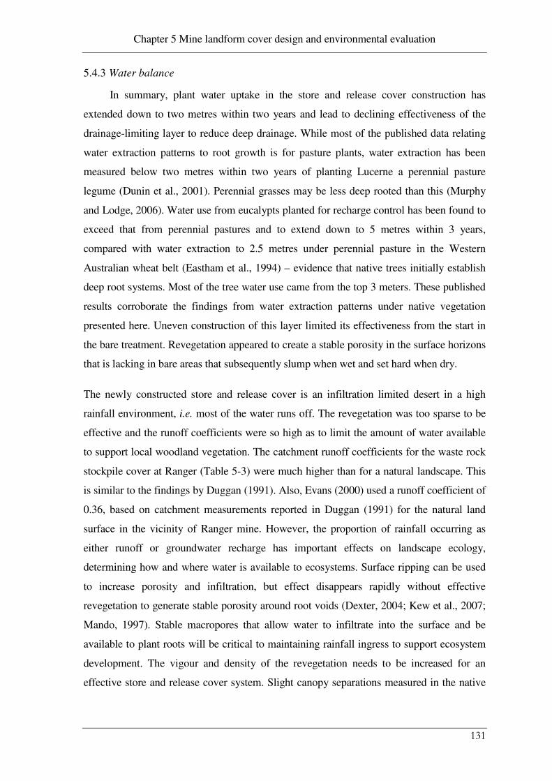
Chapter 5 Mine landform cover design and environmental evaluation
131
5.4.3 Water balance
In summary, plant water uptake in the store and release cover construction has
extended down to two metres within two years and lead to declining effectiveness of the
drainage-limiting layer to reduce deep drainage. While most of the published data relating
water extraction patterns to root growth is for pasture plants, water extraction has been
measured below two metres within two years of planting Lucerne a perennial pasture
legume (Dunin et al., 2001). Perennial grasses may be less deep rooted than this (Murphy
and Lodge, 2006). Water use from eucalypts planted for recharge control has been found to
exceed that from perennial pastures and to extend down to 5 metres within 3 years,
compared with water extraction to 2.5 metres under perennial pasture in the Western
Australian wheat belt (Eastham et al., 1994) – evidence that native trees initially establish
deep root systems. Most of the tree water use came from the top 3 meters. These published
results corroborate the findings from water extraction patterns under native vegetation
presented here. Uneven construction of this layer limited its effectiveness from the start in
the bare treatment. Revegetation appeared to create a stable porosity in the surface horizons
that is lacking in bare areas that subsequently slump when wet and set hard when dry.
The newly constructed store and release cover is an infiltration limited desert in a high
rainfall environment, i.e. most of the water runs off. The revegetation was too sparse to be
effective and the runoff coefficients were so high as to limit the amount of water available
to support local woodland vegetation. The catchment runoff coefficients for the waste rock
stockpile cover at Ranger (Table 5-3) were much higher than for a natural landscape. This
is similar to the findings by Duggan (1991). Also, Evans (2000) used a runoff coefficient of
0.36, based on catchment measurements reported in Duggan (1991) for the natural land
surface in the vicinity of Ranger mine. However, the proportion of rainfall occurring as
either runoff or groundwater recharge has important effects on landscape ecology,
determining how and where water is available to ecosystems. Surface ripping can be used
to increase porosity and infiltration, but effect disappears rapidly without effective
revegetation to generate stable porosity around root voids (Dexter, 2004; Kew et al., 2007;
Mando, 1997). Stable macropores that allow water to infiltrate into the surface and be
available to plant roots will be critical to maintaining rainfall ingress to support ecosystem
development. The vigour and density of the revegetation needs to be increased for an
effective store and release cover system. Slight canopy separations measured in the native

Chapter 5 Mine landform cover design and environmental evaluation
132
analogue area woodlands (Chapter 4) indicate that effective revegetation will provide a
fairly continuous canopy cover.
Significant changes in the soil water store of the constructed cover over a 4 year period
were associated with plant water extraction from the developing root system. While better
control over the construction of the sub-surface drainage limiting layer could improve
drainage control the layer is unlikely to remain intact unless it is installed beyond the
influence of tree roots. Similar interactions between tree roots, soil fauna and constructed
covers have occurred at other sites (Taylor et al., 2003). Based on published information on
water extraction patterns under native vegetation, drainage limiting layers may need to be
installed below 5 metres to be beyond the influence of tree roots in this environment
(Eastham et al., 1994; Kelley, 2002; Kelley et al., 2007). The thicker cover will depend on
evapotranspiration from the revegetation to control drainage otherwise persistent saturated
soil conditions at depth will drive deep drainage.
The level of control that was achieved in operational handling of weathered zone material
could not achieve layer thicknesses less than 1 metre. Increasing the thickness of the
drainage limiting layer to 2 metres could also halve the drainage flux according to water
balance modelling estimates. This design modification has wider support (O'Kane et al.,
2003). Again, the effectiveness of the revegetation in establishing transpiring leaf area will
be critical to achieving the predicted improvement in drainage control. Without effective
evapotranspiration infiltration will still flux down through a drainage limiting layer, albeit
at a slower rate.
5.4.4 Environmental support
Waste rock covers designed for ecosystem support may need to provide for plant
available water store in the surface five metres (Kelley, 2002; Kelley et al., 2007) and a
400-500 mm deficit at the end of the dry season (Cook et al., 1998). Some of this water
supply may be provided in a thicker drainage limiting layer. While the surface 2 to 3-m
contains most of the root activity, deeper profile water retention may be critical to tree
survival in periods of extreme drought. While there is evidence that over storey woodland
plants can grow well on mine waste, the eventual introduction of annual grass understorey
will significantly increase evapotranspiration demand (Hutley et al., 2001) and put
additional demand on water retention and water stress on plant communities.
Chapter 5 Mine landform cover design and environmental evaluation
133
The water balance for the ripped and revegetated monitoring plots showed enhanced
drainage initially that declined over three years. Because the cover was not effectively
revegetated the general condition was of low infiltration through a compact and massive
surface. Low infiltration through the surface acted as a throttle limiting the water available
to plant growth, a critical factor in ecosystem function (Ludwig et al., 2000a) particularly in
water limited environments (Cook et al., 2002). This constraint over plant water supply
could affect the successful establishment of comparable ecosystems to those in the
surrounding natural landscape.
In Eucalyptus tetrodonta savannas that occur widely in the natural landscape around
Ranger mine, growth of fine surface roots is restricted to the wet season and concentrated in
the upper 0.5 m (Chen et al., 2004). These roots probably supply most of the nutrients taken
up by the tree, as well as water during the wet season. However, the fine surface roots
rapidly die off during the dry season, during which tree roots can exploit the top five metres
of soil to supply transpiration requirements (Cook et al., 2003; Kelley et al., 2007). It seems
likely that evergreen eucalypts then produce fine roots at depth to access subsoil water, but
these fine subsoil roots would possibly become inactive or die during the wet season
because of elevated ground-water levels and consequent hypoxic conditions. Local water
tables rise from 7–10 m depth in the dry season up to 0.5–2 m in the wet season in
Eucalyptus tetrodonta savannas (Cook et al., 1998). Thus, evergreen water uptake may
alternate between surface fine roots in the wet season and subsoil fine roots in the dry
system. This natural, seasonal variation in phreatic water tables may not be reinstated in the
waste rock landscape without some drainage limitation at 3 to 5-m depth.
5.5 Conclusions
Cover design for ecosystem reconstruction is a special case of the store-and-release
cover where the potential water storage and drainage conditions within the root zone can
support the re-establishment of self-sustaining natural vegetation communities, typified in
the natural analogue landscape. The design of the plant growth medium needs to
demonstrate the capacity to support naturally occurring woodland ecosystems and restore a
natural water balance to the mine landscape, as well as resist erosion. The revegetation will
indirectly affect landform integrity since the evapotranspiration capacity of the

Chapter 5 Mine landform cover design and environmental evaluation
134
revegetation, and the protection it affords from rainfall erosion significantly influence
drainage flux, runoff and erosion rates.
A basic cover design concept that uses unweathered, or primary, waste rock material over
oxidised waste to provide erosion resistance, water retention for plant growth and drainage
limitation could be refined to conform with natural analogue conditions essentially by
increasing the thickness of the component layers. High energy compaction of the drainage
limiting layer may improve its performance. Surface treatment activities such as deep
ripping also need to be combined with effective revegetation. Otherwise the stable soil
porosity that is associated with biological activity and is essential for ecosystem function
will not develop.
Demonstrating similarities in ecosystem support properties between the final landform
cover and the soil zone in a natural analogue area will underpin an ecosystem restoration
methodology. Long–term monitoring (5 to 10 years) of a final landform trial designed
according to the environmental properties of natural analogue areas could improve cover
design specifications and be used to develop a predictive capacity that ensures on-site and
off-site environmental outcomes will be achievable within a particular time frame.
5.5.1 Further studies
The geomorphology, vegetation, soils and hydrology of a natural analogue area, the
Georgetown analogue area identified in Chapter 4, are described in Chapter 6 to support a
design approach for landscape restoration following mining. Landform designs can be
validated using erosion and hydro-ecological models and by checking the geomorphic and
cultural context of the landscape. However, the capacity to predict ecosystem patterns in the
reconstructed terrain is needed to demonstrate an ecological design methodology.
Consequently, a detailed study is made in Chapter 6 of environments in the a natural
analogue area selected in Chapter 4 to support species distribution models that are
developed in Chapter 7. These quantitative models can be used to assess whether a
landform design will support similar vegetation patterns to surrounding natural landscapes.

Chapter 6 Analogue landform environmental survey, design criteria and evaluation
135
Chapter 6 Analogue landform environmental survey, design
criteria and evaluation
6.1 Introduction
6.1.1 Background
Consultation and independent evaluation are front and centre of any mine closure
planning process because the context of landscape restoration has to be addressed from
several different stakeholder perspectives (ICMM, 2006). The consultation and evaluation
process has the current life of mine as the starting point. The life of mine plan accounts for
the volumes and quality of waste the capacity of pits and the schedule of operations to
closure. In this chapter, the geomorphic properties of a selected natural analogue area have
been applied to life of mine plan estimates of waste rock to design a waste rock landscape
at the Ranger uranium mine site. The design is also informed by consultation with
Traditional Owners of the land and by independent technical evaluation.
A schematic outline of the program of consultation and independent technical evaluation
leading from mine planning to construction is presented in Figure 6-1.
Figure 6-1 Landform design process, numbered circles
indicate consultation points

Chapter 6 Analogue landform environmental survey, design criteria and evaluation
136
This is an iterative process that is recommenced following significant changes to the mine
plan. The stages of the program that were completed in this thesis are highlighted in green
in Figure 6-1. Points of consultation are indicated by numbers in Figure 6-1.
6.1.2 Landscape design
Relief and hillslope morphometry are topographic properties of an ecosystem, which
when integrated with stable soil and the plant communities, connect the surrounding
ecosystems (Carpenter, 1998). Thus topography, soil and vegetation can be reconstructed
together to optimize the restoration of key ecological processes. The methodological
development being proposed here is therefore to design mine landform relief and hillslopes
from the grain size and extent attributes of natural analogue landforms that were
investigated in Chapter 4. The purpose is to restore natural ecosystem patterns and
environmental processes at the landscape level. However, the analogue natural ecosystems
need to be described in sufficient detail to support the design process and validate species
distributions in the reconstructed landscape.
The focus on ecological objectives is aimed to differentiate the proposed methodology
conceptually from hydrological approaches to topographic reconstruction, such as the basin
relief approach (Toy and Chuse, 2005). The latter is directed primarily to protecting the off-
site receiving environment rather than the quality of the on-site environment after mine
closure. Although reference, or analogue sites, are used routinely to set closure criteria for
mine rehabilitation following opencast mining (Bell, 2001), this approach lacks landscape
ecological context. A range of ecological landform design methodologies have been
proposed that recommend physical evaluation methods based on numerical erosion and
hydrological models (Nicolau, 2003; Toy and Chuse, 2005). Previous studies assert that
methods to restore natural biodiversity in mined landscapes need to be developed
(Ehrenfeld, 2000; Ehrenfeld and Toth, 1997).
The failure of the ecological design may be partly due to complex ecosystem composition
and variation (Holl et al., 2003). However, analytical approaches that have become widely
applied in landscape ecology, conservation biology and wildlife management have yet to be
adopted in restoration ecology. The grain size and extent attributes of ecological scale in
landscapes that were used in Chapter 4 to identify analogue landforms and describe
underlying environmental processes of erosion-sedimentation and water distribution are

Chapter 6 Analogue landform environmental survey, design criteria and evaluation
137
applied here to geomorphic design of the waste rock landform. This will partly address the
issue of a lack of ecological context. The critical aspects of cover design or soil
reconstruction affecting plant available water and drainage that were identified in Chapter 5
also need to be understood.
6.1.3 Soils on waste rock and natural analogues
The waste rock materials at Ranger are generally richer in P and have lower in N than
natural soils in the area (Ashwath et al., 1994). The rock materials can occasionally be
saline and in some situations may produce acid drainage with high metal concentrations
(Mg, Mn, U and Pb), as evident in Chapter 5. Salinity caused by magnesium sulfates
produced from weathering of primary rock material has been found at levels not toxic to
plants (Ashwath et al., 1994). However, tolerant plant species may be required in situations
where there is drainage discharge.
The retention of nutrients is a key measure of ecological integrity (Ludwig et al., 2004), as
nutrient fractions such as labile or plant available phosphorous, a limiting factor for the
establishment of woodland savanna ecosystems (Short et al., 2000), tend to be concentrated
in the topsoil under natural woodland. The retention and recycling of nutrients are closely
linked to amount of organic matter in the near surface of soils overlying deep weathered
regolith that supports eucalypt woodland (Koch and Hobbs, 2007; Schwenke et al., 2000a).
The soil morphological patterns associated with drainage status were observed to be linked
to gradients in woodland vegetation type. Past studies of root distribution in northern
savanna woodlands indicate that 70% of the root biomass is at < 0.2 m soil depth and the
rest of the root mass is accounted for between 0.3 < 1.4 metres (Werner and Murphy,
2001). Although, the dry season water extraction patterns occur predominantly in the top 2
metres some water extraction can occur below 4.5 meters (Chen et al., 2004; Kelley et al.,
2007). Also, the morphologies of gradational texture profiles and rocky soils were not
inconsistent with soil design specifications that have been produced for erosion resistant
covers that use a mix of materials to produce erosion resistance, drainage control and
growing medium for plants over uranium milling waste (Johnson, 2002). This concept
seems compatible with the analogue soil morphology — described in Chapter 4 — as
massive and earthy, gravelly, sandy loams at the surface to sandy clay loams at depth, with

Chapter 6 Analogue landform environmental survey, design criteria and evaluation
138
a root-limiting layer in the form of weathered rock or ferricrete hardpan within 1.5 to 3.0- m
of the land surface.
6.1.4 Eco-hydrology
Eco-hydrology is an important aspect of mine-site rehabilitation (Section 2.5.3). The
interactions between groundwater and surface water in the natural landscape occur mainly
in the surface five metres (Vardavas, 1993) where woodland vegetation is consuming a
major part of the available water through evapotranspiration (Cook et al., 2002; Hutley et
al., 2000). However, the hydraulic conductivity in the subsoil in the waste rock would be
much higher than in the natural regolith where there is a conductivity throttle at 2 – 3
metres below the surface that generates throughflow to the creeks (Vardavas, 1993). The
hydraulic conductivity throttle in the natural regolith is analogous to the drainage-limiting
layer in the constructed landform cover evaluated in Chapter 5. The water balance of the
shallow hydrological system may determine the ecological outcomes. The shallow
hydrological system needs to be placed in perspective and reasonable bounds on the
components of the water balance need to be set with respect to the natural environment and
what may happen following rehabilitation.
A significant hydrological study of eucalypt woodland in the Northern Territory was
undertaken at Howard Creek near Darwin between 1996-98 (Cook et al., 1998; Hutley et
al., 1997; Kelley, 2002). The Howard Creek study measured the evapotranspiration (ET)
components of the water balance and used these to estimate the rates of groundwater
recharge. The technique involved heat-pulse monitoring of overstorey transpiration,
chamber estimates of understorey transpiration and soil evaporation, and then the total ET
measurement was obtained via eddy covariance. There was also some measurements of soil
water dynamics (Kelley et al., 2007). Cook et.al. (1998) undertook a hydrographic water
balance that differed from that of Hutley et.al. (2000). These differences are summarised in
Table 6-1.
Another study was done by Cook et al. (1998) in which they estimated ET from
interpretation and rescaling of catchment and groundwater hydrographs rather than direct
measurements. Hutley et al. (2000) reported the actual measurement results, but their study
did not extend beyond ET and a limited number of soil water dynamics measurements and
their ET rates appear to be underestimated. The total ET of 1,110 mm.yr-1
estimated from

Chapter 6 Analogue landform environmental survey, design criteria and evaluation
139
the catchment water balance by Cook et al. (1998) was higher. However, the Hutley et al.
(2000) measured interception separately (88 mm.yr-1
) while Cook et al. (1998) lumped
interception into their total ET. Consequently, the combined understorey and soil
evaporation of Cook et al. (1998) and Hutley et al. (2000) were similar (Table 6-1).
Vardavas (1998) outlined a parametric model of the Magela Creek catchment, where
Ranger mine is located, and observed that interflow was important in stream flow
generation. This study concurs with the fact that interflow can be a larger component of
stream flow than surface runoff. This study also reported that the wet season runoff was
saturation controlled by a variety of below-ground processes, including interflow, soil-
water-storage capacity and bedrock percolation rates.
Table 6-1 Comparison of water balance estimates at
Howard Creek reported by (Cook et al., 1998) and
(Hutley et al., 2000)
Component (Cook et al., 1998)
(mm.yr-1)
(Hutley et al., 2000)
(mm.yr-1)
Rainfall 1 720 1 750
Overstorey – wet season transpiration 370 160
Overstorey – dry season transpiration 175 153
Overstorey total transpiration 545 313
Understorey and soil evap. – wet season 440 381
Understorey and soil evap. – dry season 125 176
Total understorey and soil evaporation 565 557
Leaf interception 0 88
Total ET (sum of above ET components) 1 110 958
Stream flow 590 590
Net groundwater recharge 20 —
Residual (rain – ET – flow – recharge) 25 202
Stated study uncertainty -20 to +120 —
Previously, Vardavas (1993) reported that a reasonable volume of water enters and leaves
the groundwater system each year (150 to 200 mm.yr-1
) virtually all the water movement
was vertical with water entering as rainfall during the wet season and being lost as ET
during the dry season. Woods (1994) estimated similar natural recharge rates in the order of

Chapter 6 Analogue landform environmental survey, design criteria and evaluation
140
65 to 130 mm.yr-1
(5 to 10% of rainfall) under natural conditions from a drawdown analysis
of the Jabiru town water supply bore field (Pidsley 1990).
6.1.5 Ecosystem survey support
The ecological outcomes of a mine landform design need to be predictable in order to
validate the landform design being proposed (Nicolau, 2003). The number of observations
and the range and scale of analogue landscape variation would be factors in designing
ecosystem surveys to support predictions. Landscape topography can spatially influence
patterns of water loss and accumulation thereby dampening or amplifying vegetation
patterns (Ben Wu and Archer, 2005). Therefore, a grid survey design with a site spacing
that is a fraction of the flow path length from crest to valley floor should resolve variation
in hill slope environments that affect plant species distribution.
Resolution of the hill slope factors causing environmental variation probably requires a
minimum of 100 survey observations (Stockwell and Peterson, 2002). The common and
abundant species that account for most of the ecosystem space also need to be identified, as
these species will contribute the most value to the rehabilitation design. Collecting species
abundance data requires additional effort to recording presence absence. Detailed study
plots and plant area counts are needed. Environmentally stratified sampling designs have
been used to assess spatial organisation of ecosystems in landscapes (Ludwig and
Tongway, 1995; Rempel and Kushneriuk, 2003). The six ecosystem types identified in
Chapter 4 could be used to select representatives from the grid survey observations across
the analogue landform, thereby ensuring that plant community descriptions had an explicit
landscape context with the mine landscape restoration task.
6.1.6 Erosion
Rainfall in the Alligator Rivers Region is some of the most intense and erosive in
Australia, and hence water erosion is a significant process (Duggan, 1991) that needs to be
addressed in rehabilitation design. In such a situation, average denudation rates may not
accurately reflect the risk to containment integrity from gully erosion. The Australian
guidelines for the construction of covers over radioactive waste material recommend a
structural life of at least a 1 000 years (Anon, 1987). To meet these guidelines, a sediment
transportation model is required. SIBERIA is a deterministic three-dimensional erosion and

Chapter 6 Analogue landform environmental survey, design criteria and evaluation
141
sediment transport model, which can be used to simulate topographic evolution over long
periods based on transport limited erosion rates (Willgoose et al., 1991).
The SIBERIA erosion model has been calibrated for materials and conditions at Ranger
uranium mine (Evans et al., 2004; Evans and Willgoose, 2000; Willgoose and Riley, 1998)
and elsewhere (Boggs, 2003; Hancock et al., 2000; Hancock et al., 2008; Hancock and
Turley, 2006) to assess containment risks associated with the final landform design. The D8
flow routing algorithm used in SIBERIA to route surface runoff is a computational
simplification that does not accurately represent overland flow divergence and soil water
conditions (Wilson et al., 2005). While SIBERIA may not accurately represent variation in
soil conditions, it nevertheless describes how a catchment would look, on average, at a
given time. It is thus used as a tool for validating landform designs (Hancock et al., 2008;
Hancock and Turley, 2006).
The aims of this chapter were twofold: (i) develop and undertake independent validation of
a landform design for closing Ranger uranium mine; and (ii) describe the ecological context
for the waste rock landform based on the environmental patterns in a selected natural
analogue area.
6.2 Methods
6.2.1 Ranger mine landscape
An oblique air photo of the Ranger mine site obtained in 1974 (Plate 6-1) before
mining began shows the site to be located on a peneplanated surface, bounded by streams
and backed by high relief sandstone plateau. Another aerial oblique photo of the site taken
in 2001 and looking north (Plate 6-2) shows land use associated with the operating mine
including waste rock stockpiles, open pits, ponds, tailings storage facility and industrial
facilities. This gives an indication of the extent of the restoration task. An outline of the
proposed design and evaluation process that refers to the Ranger mine site and follows the
scheme presented in Figure 6-1 is developed in the sections that follow.
Ranger mine has important indigenous owner land use values. Ecosystem reconstruction is
important to the Mirrar traditional owners of the Ranger mining lease. The results of initial
consultation with the Mirrar on their expectations for landscape reconstruction and
revegetation set the boundary conditions for landscape restoration at this site. Consultation

Chapter 6 Analogue landform environmental survey, design criteria and evaluation
142
on the broad vision for landscape reconstruction was made with the Traditional Owners and
their representatives (Gundjehmi Aboriginal Corporation and the Northern Land Council)
In a site visit to the Georgetown analogue landform area (identified in Chapter 4) in 2002
the Mirrar verbally supported the vision of the rehabilitated final landform. The next (but
first recorded) consultation on the closure process with the Mirrar occurred in 2005 at Mula
in Kakadu National Park. Final land use objectives were discussed including aspects of
final landform scheduling, backfilled pit landforms, land surface rockiness, tailings storage
facility rehabilitation and water course reinstatement. The Mirrar placed particular
emphasis on the following issues: (i) leaving no additional water bodies; (ii) providing a
land surface that would support hunting and gathering activities; and (iii) reinstating
woodland plants.
Plate 6-1 Oblique air photo of the Ranger site to the
south before mining began
An extract from the summary notes from the meeting included the following statement:
“A stable, natural environment that is safe to access and capable of sustaining the variety
of animals and vegetation (including native food and medicinal species) endemic to the
surrounding environment. The preferred underlying landform would be as flat and low in
relief as possible to minimise the possibility of erosion.”
Magela Creek
Gulungul Creek
Pit 3
Pit 1

Chapter 6 Analogue landform environmental survey, design criteria and evaluation
143
Plate 6-2 Oblique air photo of the Ranger site to the
north in 2001
6.2.2 Landform design
Landform design criteria at the Ranger mine case study site were derived from the
central tendency and dispersion measures of terrain attributes in the Georgetown analogue
area. The design criteria were applied to mine planning estimates to draft a mine landform
design. The geomorphic similarity of the landform design to the natural landscape was then
evaluated. Published landscape evolution modelling and hydro-ecological modelling
methods were used by independent investigators to assess whether the landform design
restored natural erosion and water balance processes. In addition, a detailed environmental
survey of the Georgetown analogue area is made and vegetation presence-absence,
abundance, and soil properties described to support ecological modelling in Chapter 7.
6.2.3 The natural analogue areas
A method, used for selecting the natural analogue areas and identifying the ecosystem
gradients with reference to the scale and geomorphology of the mine landscape, was
developed in Chapter 4. Two analogue landforms were selected — similar in shape, size
and habitat complexity to the final landform — and the environmental range was classified
into six ecosystem types on rocky substrates. One analogue landform, Georgetown, a rocky
rise southeast of the mine was preferred because it comprised a complete range of
Pit 3
Pit 1
Stockpiles
tailings storage facility

Chapter 6 Analogue landform environmental survey, design criteria and evaluation
144
environmental variations of the rocky substrates that could be incorporated into the mine
landform. Thus the natural analogue selection was based on a reconnaissance survey to
identify the context and range of environmental variations appropriate to reconstruction of
the mine landscape.
6.2.4 Topographic reconstruction
Assuming the natural landscape is in equilibrium with environmental conditions, then
the acceptable gradients of the landform design properties can be set from their numeric
ranges obtained from the natural analogue area. Toy and Chuse (2005) proposed a mine
landform design method that restored drainage-basin area, weighted mean slope, and
drainage density for the pre-disturbance or analogue landscape. A major limitation of their
proposal is that the selection process for the analogue areas was not specified. However, the
proposed major focus of this thesis was to use digital terrain analysis and computer aided
design techniques to create “steady state” landscape configurations typical of mature
natural landforms. Another limitation is that soil properties are not specified. A problem
with specifying soil property development in waste rock is that there will be changes over
time (see Chapter 5). There have been recent developments in predicting soil formation
from parent materials in hillslope environments from erosion, sedimentation and mineral
weathering processes(Minasny et al., 2008). However, these are yet to be applied to
landscape restoration.
The design methodology developed here differs from Toy and Chuse (2005) in that it is
iterative and specifies the environmental range in an analogue area (Chapter 4) and uses
terrain properties from terrain analysis to incorporate scale dependent ecological processes
rather than average catchment characteristics. In this methodology the primary terrain
attributes (Table 4-1) related to the landscape energy level, geomorphic processes (Allen et
al., 2003), erosion, sedimentation and drainage (Moore et al., 1991) were specified from the
natural analogue area. As digital terrain attributes tend to be non-normally distributed
(Gallant and Wilson, 1996), the central tendency and acceptable range in landform criteria
were defined more reliably from non-parametric measures such as median and quantile
distribution.

Chapter 6 Analogue landform environmental survey, design criteria and evaluation
145
6.2.5 Terrain analysis
The construction of the elevation grid (DEM) was described in Chapter 4. A range of
topographic parameters: erosion and sedimentation indices, wetness index, relief,
catchment size, slope, flow path length, and landscape curvatures were used to describe
variation in the physical environment that supports ecological diversity. Slope length is an
important parameter that is very difficult to measure because it can be measured from
different start and end points (Renard et al., 1997). The flow path length in TAPESG was
applied here. This flow length measure is the longest flow path at a point, i.e. it is the
longest distance to the catchment divide. Curvature is an important landform attributes that
affects slope stability (Hancock et al., 2003) and water and sediment distribution in
hillslope environments.
There are two types of curvature measurement. The first is profile curvature is the curvature
of the surface in the direction of maximum downward slope, that is, along the flow line
through a point. A second type is the plan curvature, which is the curvature of a contour
drawn through a point. In general, curvatures are determined by the reciprocal of the radius
of a curve. A gentle curve has a large radius and hence a low curvature, while a tight curve
has a small radius and large curvature. As the curvature values are small, so they are
multiplied by a hundred to give more comfortable values. The units of curvature are radians
per metre, the change in orientation typically measured by travelling 1 metre along the
respective line. Curvature values are typically less than one and are multiplied by 100 for
easier interpretation. Thus a curvature of 5 is 0.05 1/metres, and corresponds to a radius of
20 metres. Negative curvature values represent concavity and positive values convexity.
The upslope contributing area, measured in square meters, is the area contributing runoff
flow at a point in the landscape. TAPESG calculates this area from flow path and flow
accumulation in the landscape. The FD8 or Rh08 flow routing algorithms are implemented
in TAPESG allowing flow dispersion to be represented. Flow is distributed to multiple
nearest-neighbour nodes in upland areas above defined channels and D8 or Rho8
algorithms below points of presumed channel initiation. Based on visual assessment of
high-resolution air photography in the analogue landform, an area of 10 000 m2 to define
stream channel initiation was used. A maximum cross grading area of 10 000 m2 was used
that corresponded with the area defining stream channel initiation. The cross-grading

Chapter 6 Analogue landform environmental survey, design criteria and evaluation
146
algorithm is applied when the contributing area is less than the cross-grading threshold. In
low relief landscapes, this prevents dispersion of flow lines in the bottom of valleys.
6.2.6 Environmental evaluation of the reconstructed landform
In order to compare the landscape attributes of the analogue and reconstructed
landform, a terrain model of the mine landform that was based on the life of mine plan
estimates of pit and waste volumes that were valid in 2001was created was created using
Vulcan (Maptek) mine planning software. The quantity of material remaining on the land
surface after the backfill of the pits consisted of 17.41 Mm3 of non-mineralised (< 0.02%
U3O8) material and the tailings dam walls, which currently form a water retaining structure.
Pre-existing catchment boundaries were reinstated and non-mineralised stockpiles were re-
contoured according to the design guidelines to create a draft design that comprised water-
shedding waste rock landforms. Primary terrain properties of elevation, slope and curvature
that were based on their ranges in the Georgetown analogue area were used as topographic
design criteria. The range of the elevation and slope specifications was slightly widened to
allow for consolidation over time in the backfilled pits.
6.2.6.1 Terrain evaluation
The landscape attributes of elevation, slope, wetness index, erosion index (LS factor
from the USLE erosion model), and stream power index and plan curvature in the built
landscape were compared to their range in the surrounding natural landscape. These indices
were selected to describe the energy level of the landscape and the patterns of water,
sediment and erosion distribution that defined landscape dynamics and ecosystem function.
A perspective view of the reconstructed landform showing different digital terrain attributes
in the analogue area was checked visually in ArcGIS. The quartiles of the distribution of
analogue terrain attributes were mapped to identify values that were outside the analogue
area range and the design was modified.
6.2.6.2 Landform evolution
Landform evolution over 1000 years for a DEM that comprised the post-mining
landform and the Georgetown analogue landform was independently assessed using the
SIBERIA model (Lowry et al., 2006). The DEM of the proposed post-mining landform had

Chapter 6 Analogue landform environmental survey, design criteria and evaluation
147
to be resampled to ensure that it fell within the grid array limitations (250 cells by 250 cells)
of the SIBERIA program (Willgoose and Riley, 1998). The locations of catchment outlets
from the drainage network generated from the DEM were identified. Also in the process,
two surface conditions were applied: areas which had a slope of greater than 10%, which
were regarded as being likely to be treated with rock batters and mulching; and the
remainder of the area was regarded as possessing ‘natural’ characteristics. Erosion and
hydrology parameter values from Evans (2000) were used to describe the surface condition
of each of the two areas.
6.2.6.3 Ecohydrological evaluation
An independent evaluation of catchment water balance was made for a DEM
comprising the post mining landform and the Georgetown analogue landform using WEC-
C (Croton and Dalton, 2006), a distributed deterministic catchment model (Croton and
Barry, 2001) that simulates stream flow generation from runoff and below ground
processes, i.e. interflow and groundwater discharge. The model was described in detail by
Croton and Barry (2001) and has been applied in a range of eucalypt woodland
environments to assess ecohydrological effects of mine rehabilitation (Croton and Reed,
2007), land clearing (Croton and Bari, 2001) and forestry development (Bubb and Croton,
2002). WEC-C is particularly useful for mining studies in that it can incorporate soil
excavation, and other profile changes, as inputs during the simulation. The unit of time for
input of evaporation and rainfall data is daily; however, to maintain stability and accuracy
the model operates on an hourly internal time-step.
Initial modelling of possible soil and vegetation covers for the rehabilitation of the Ranger
mine used a simple one-dimensional (1-D) model of the profile. This modelling indicated
the likely range of water balance components for the rehabilitated mine. A weakness of 1-D
modelling is that interflow is not allowed and so outputs are restricted to ET, surface runoff
and deep recharge. The soil layering for the base case used in 1-D modelling of the soil
profile is shown in Table 6-3. These characteristics were partly based on information from
the landform trial results reported in Chapter 5 and on experience with the WEC-C model
in eucalypt woodland environments in south Western Australia.

Chapter 6 Analogue landform environmental survey, design criteria and evaluation
148
Table 6-2 Parameters for the base-case 1-D model
Layers
Total Thickness
(m) Soil Type Ks (mm/day) Vegetation Roots
1 & 2 1.0 cover 50 yes
3 & 4 1.0 clay liner 10 yes
5 to 7 3.0 waste rock 24,000 yes
8 to 11 7.0 subsoil 10 yes to 8m
12 3.0 drainage layer 10 no
The soil profile given in Table 6-3 was run for four vegetation cases, each having an annual
sinusoidal variation in LAI (leaf area index) to reflect the growth and senescence of
vegetation through the wet and dry seasons. The base case had an LAI of 0.8-1.6 from
overstorey and understory LAI reported by Hutley (2000). To test sensitivity to LAI, three
cases using simple ratios of this base case were simulated: 0.4-0.8 (half base), 0.6-1.2 (three
quarters base) and 1.0-2.0 (one and a quarter base). The model was also run for four
variations of Ks for the clay drainage limiting layer: 5 mm.day-1
, 10 mm day-1
(base case),
20 mm day-1
and 40 mm day-1
.
The 3D water balance model formulation was based on a combination of the
parameterisation of the WEC-C model for natural, uncovered areas, comprising a
catchment called Corridor Creek and with the parameterisation of the 1D mine
rehabilitation WEC-C model for the covered areas. Corridor Creek is a monitored
catchment on the southern side of the Ranger mine that has been affected by the mining
operations — there are wetland filters, small dams, as well as sections of a tailings dam and
a mine pit within the catchment. There has also been controlled release of mine water into
the catchment. The gauged catchment is 257 hectares in area and stream flow data was
available from 1 Jan 1994 until 14 Apr 2003. The total area of the simulated catchment is
306 hectares.
The initial WEC-C 3D model was prepared for the Corridor Creek catchment at a 50-m
grid spacing and a six layer profile. Water flow in Corridor Creek is a combination of
surface runoff during intense rainfall events and near-surface interflow during the balance
of the wet season. Generally flows cease by early May for all years in the period 1994 to
1998; this implied that deep groundwater made little or no contribution to stream flow and

Chapter 6 Analogue landform environmental survey, design criteria and evaluation
149
that stream flow depended on surface runoff and interflow. This model of the groundwater
system was consistent with the studies by Vardavas (1993).
6.2.7 Environmental surveys
Two environmental surveys of vegetation and soils were made to establish: (i) plant
species distribution; and (ii) soil morphology and soil physical and chemical characteristics
that are important to ecosystem reconstruction. Firstly, a grid survey of the Georgetown
analogue landform (500 hectares) was undertaken to describe soil morphology and species
presence–absence. A grid spacing of 200 metres was used to sample 102 sites. This spacing
gave a resolution that was similar to the third quartile of the range in slope lengths
(160 metres), i.e. one quarter of the slope lengths in the analogue area were longer that the
grid spacing and three quarters were shorter. Some resolution of hill slope variation may
have been lost, however this spacing produced a reasonable number of sites to survey in the
time available and was well within the range of hill slope lengths (300 – 400 m).
At each site the woodland vegetation was visually classified (based on the dominant
overstorey species) into 1 of the 6 ecosystem types on rocky substrates (Table 6-4)
determined from the multivariate analysis in Chapter 4. Soil morphology was described at
each site according to standard methods (McDonald et al., 2009) from auger profiles down
to contact with the substrate or 1.5 metres, whichever was shallower.
Table 6-3 Six vegetation communities on schist
derived substrates in the Georgetown analogue area
Ecosystem type code Ecosystem type description
3 Tall Eucalyptus tetrodonta/E. bleeseri/mixed open woodland with a sparse mixed tree midstorey and mid-dense Sorghum intrans/Petalostigma quadriloculare understorey.
4 Mid-high Melaleuca viridiflora open woodland with a very sparse mixed tree midstorey and dense mixed grass/Cyperaceae understorey.
6 Tall Eucalyptus tetrodonta/E. miniata open woodland with a sparse mixed tree midstorey and mid-dense Heteropogon triticeus/Sorghum intrans understorey.
7 Tall Eucalyptus tetrodonta/E. miniata/E. porrecta open forest with a sparse mixed tree midstorey and mid-dense Sorghum intrans/Petalostigma quadriloculare understorey.
8 Tall Eucalyptus foelscheana/mixed open woodland with a sparse mixed tree midstorey and sparse Heteropogon triticeus/Themeda triandra understorey.
9 Mid-high Eucalyptus tectifica/E. tetrodonta/E. confertiflora open woodland with a sparse mixed tree midstorey and sparse Sorghum intrans/Eriachne sp. /Petalostigma quadriloculare understorey.

Chapter 6 Analogue landform environmental survey, design criteria and evaluation
150
Secondly, three representative sites of each ecosystem type listed in Table 6-4 were
randomly selected from the survey grid to provide detailed information on plant species and
abundance and soil chemical and soil physical properties. A replicated plot design was used
that comprised 3, 20 x 20-m permanent quadrats that were marked at the centre with a steel
post and the location recorded with a hand held GPS.
The ecology of plant communities was characterised in terms of community structure, plant
diversity and abundance. A biodiversity index for each of the ecosystem types is presented.
Common species were tabulated with an importance index and an indication of the range of
their occurrence across ecosystem types. Ecosystem structure, including plant density and
ground cover information for each stratum were described.
Vegetation community composition and structure was described in terms of overstorey,
mid-storey and groundcover strata. Overstorey was defined as those trees greater than 8
metres high. Midstorey was characterised as the 2-4 metre layer and understorey comprised
all plants below 2 metres. Overstorey canopy cover, species, height, health and diameter at
breast height (DBHOB) for each individual tree over 2 metres was recorded. Understorey
measurements of species, density and foliage projective cover were made in 10, 1 x 1 metre
quadrats evenly spaced along two transects running through the larger quadrat.
Furthermore, the framework species were identified in terms of their dominance in
overstorey, mid-storey and groundcover strata of each ecosystem type. Dominance was
assessed from: (i) coverage (basal area or projected foliage cover), which is a measure of
the amount of space occupied by individuals of a given species; (ii) density (number of
stems or individuals per unit area), which is a measure of the numerical dominance relative
to other species; and (iii) frequency (how many samples contain individuals of a given
species), which is a measure of the commonness of the species.
A standard suite of soil properties reflecting soluble and cation exchange chemistry and
organic matter content were measured to characterise soil fertility in vegetation plots. Two
additional sites in Melaleuca viridiflora open woodland (ecosystem type 4 described in
Chapter 4) were sampled in the soil survey to make 20 sites in total. The depth increments
were selected with respect to rooting patterns of woodland plants (Chen et al., 2004;
Werner and Murphy, 2001). The sampling and analysis plan are presented in Table 6-4.
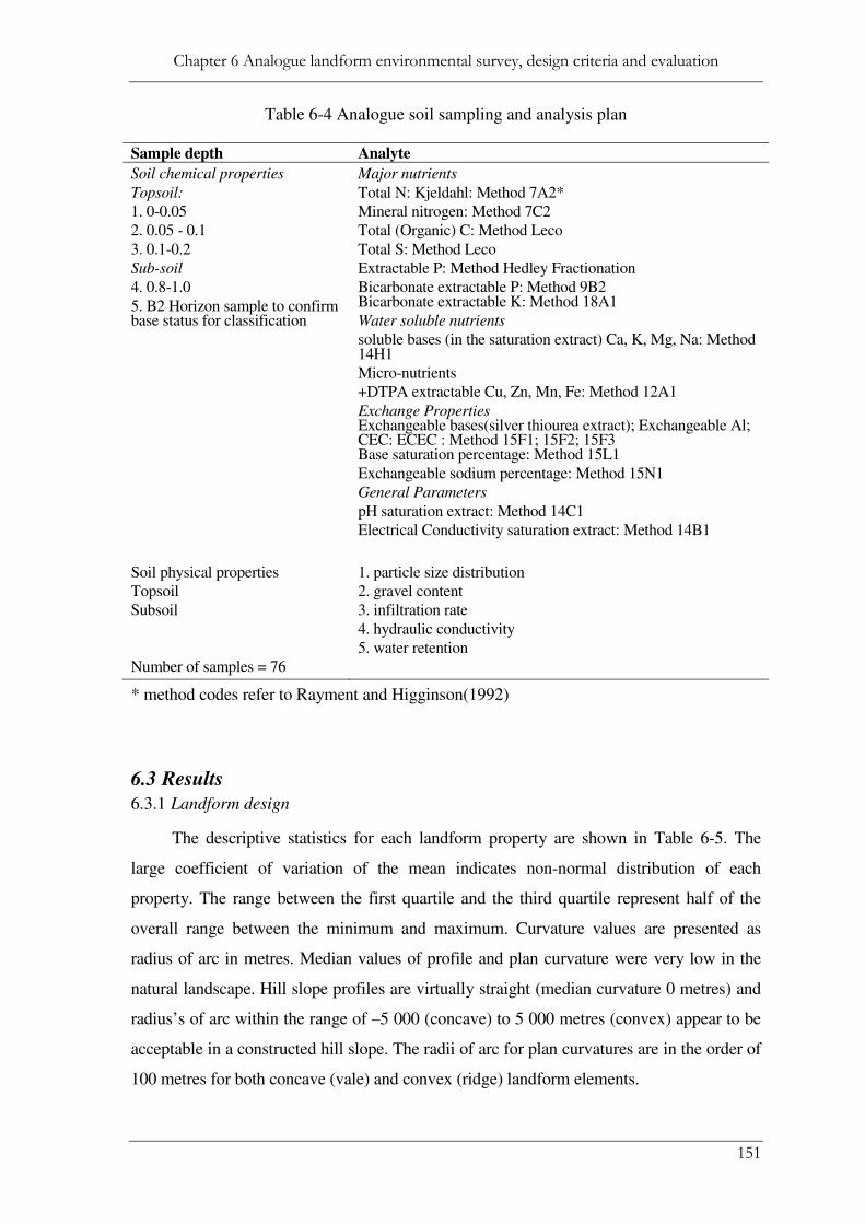
Chapter 6 Analogue landform environmental survey, design criteria and evaluation
151
Table 6-4 Analogue soil sampling and analysis plan
Sample depth Analyte
Soil chemical properties
Topsoil:
1. 0-0.05
2. 0.05 - 0.1
3. 0.1-0.2
Sub-soil
4. 0.8-1.0
5. B2 Horizon sample to confirm base status for classification
Major nutrients
Total N: Kjeldahl: Method 7A2*
Mineral nitrogen: Method 7C2
Total (Organic) C: Method Leco
Total S: Method Leco
Extractable P: Method Hedley Fractionation
Bicarbonate extractable P: Method 9B2 Bicarbonate extractable K: Method 18A1
Water soluble nutrients
soluble bases (in the saturation extract) Ca, K, Mg, Na: Method 14H1
Micro-nutrients
+DTPA extractable Cu, Zn, Mn, Fe: Method 12A1
Exchange Properties Exchangeable bases(silver thiourea extract); Exchangeable Al; CEC: ECEC : Method 15F1; 15F2; 15F3 Base saturation percentage: Method 15L1
Exchangeable sodium percentage: Method 15N1
General Parameters
pH saturation extract: Method 14C1
Electrical Conductivity saturation extract: Method 14B1
Soil physical properties
Topsoil
Subsoil
Number of samples = 76
1. particle size distribution
2. gravel content
3. infiltration rate
4. hydraulic conductivity
5. water retention
* method codes refer to Rayment and Higginson(1992)
6.3 Results
6.3.1 Landform design
The descriptive statistics for each landform property are shown in Table 6-5. The
large coefficient of variation of the mean indicates non-normal distribution of each
property. The range between the first quartile and the third quartile represent half of the
overall range between the minimum and maximum. Curvature values are presented as
radius of arc in metres. Median values of profile and plan curvature were very low in the
natural landscape. Hill slope profiles are virtually straight (median curvature 0 metres) and
radius’s of arc within the range of –5 000 (concave) to 5 000 metres (convex) appear to be
acceptable in a constructed hill slope. The radii of arc for plan curvatures are in the order of
100 metres for both concave (vale) and convex (ridge) landform elements.

Chapter 6 Analogue landform environmental survey, design criteria and evaluation
152
The relief and curvature properties of the natural landscape were used as geomorphic
design criteria by the Ranger mine department to produce a stockpile and backfill 3D model
that accounted for waste from mining and processing, and void volumes in backfilled pits.
Table 6-5 Descriptive statistics for terrain properties
in the Georgetown analogue area
Variable Units Mean Coeff.
Variation
(%)
Minimum Median Maximum 1st Quartile 3
rd Quartile
slope (%) % 2.0 50 0.0400 2.0300 6.4300 1.2500 2.7500
elevation (m) m 9.3 50 0.0 8.7600 22.6300 5.5200 12.5275
profile curvature radius (m) -12,500 na -250 0.0 400 -5,000 5,000
plan curvature radius (m) 11,111 na -0.4 1000 1 -100 83
flow length (m) m 149 205 0.0 60.0 3596.5 20.0 169.7
LS factor1 0.55 200 0.0 0.3 22.2 0.1 0.6
erosion/deposition -0.1 na -572.0 -1.0 503.0 -3.0 0.0
catchment area m2 25300 622 400 2943 2793817 1613 4974
1 slope length and steepness factor from the universal soil loss equation (Renard et al.,
1997)
The landform design criteria given in Table 6-6 were based on the measured ranges in
terrain properties in the natural analogue area (Table 6-5). Elevation and slope criteria used
in Table 6-6 were slightly higher than the maximum values in the analogue area. This was
needed to allow for 10 metres of subsidence in the backfilled pits.
Table 6-6 Landform design criteria
Variable Units Range
slope (%) % 0 – 6.5
relief (m) m 25
profile curvature radius (m) -5000 (concave) to 5000 (convex)
plan curvature radius (m) -100 (vale) to 100 (ridge)
6.3.2 Design evaluation
The three dimensional perspective views of the landform parameters elevation and
slope shown in Figure 6-2 depict ranges of these parameters in broad landscape surveyed in
Chapter 4, the Georgetown analogue area used to develop design criteria and the waste rock

Chapter 6 Analogue landform environmental survey, design criteria and evaluation
153
landform produced by the Ranger mine department. The quartile ranges in both parameters
are indicated by different colours in Figure 6-2.
Elevation
Slope
Legend
1st quartile
2nd quartile
3rd quartile
4th quartile
outside the range in the Georgetown analogue area
Georgetown analogue area extent
waste rock landform extent
Figure 6-2 Three dimensional perspective views of
terrain properties highlighting analogue area ranges
The inter-quartile range in slopes was associated with hill slope environments. Elevation
and slope parameters were slightly out of range of the Georgetown analogue area. A

Chapter 6 Analogue landform environmental survey, design criteria and evaluation
154
magenta shading indicates slopes and elevations in the final landform design and the
broader landscape that are outside the range of these parameters in the Georgetown
analogue area. Erosion issues associated with these areas of the landform design are
highlighted in subsequent independent evaluation of erosion.
The reconstructed terrain appeared to be similar in oblique aerial view to the pre-mining
landscape (Plate 6-3).
Plate 6-3 Ranger mine area air photo before (top) and
after (bottom) computer simulated view (south)
Pit 3 backfill
Pit 1 backfill
Pit 1
Pit 3

Chapter 6 Analogue landform environmental survey, design criteria and evaluation
155
Viewing a computer rendered image of the landscape design with the 2001 mine landscape
(Plate 6-4) confirmed the backfilling of the pits, reshaping of residual waste stockpiles and
the tailings storage facility and the removal of mine water ponds.
Ten meters of surcharge of waste rock over the Pit 1 backfill created a steep batter slope in
the foreground of Plate 6-4.
Plate 6-4 Ranger mine in 2001 (top) and reconstructed
landscape visualisation (bottom) – north view
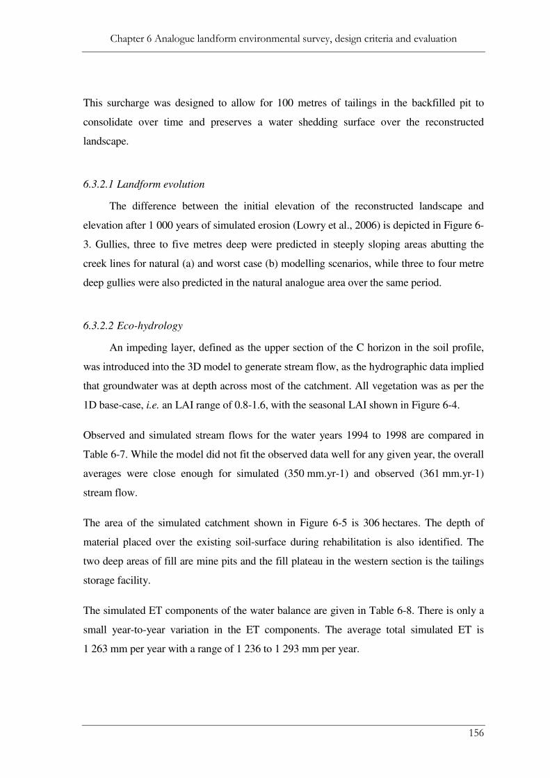
Chapter 6 Analogue landform environmental survey, design criteria and evaluation
156
This surcharge was designed to allow for 100 metres of tailings in the backfilled pit to
consolidate over time and preserves a water shedding surface over the reconstructed
landscape.
6.3.2.1 Landform evolution
The difference between the initial elevation of the reconstructed landscape and
elevation after 1 000 years of simulated erosion (Lowry et al., 2006) is depicted in Figure 6-
3. Gullies, three to five metres deep were predicted in steeply sloping areas abutting the
creek lines for natural (a) and worst case (b) modelling scenarios, while three to four metre
deep gullies were also predicted in the natural analogue area over the same period.
6.3.2.2 Eco-hydrology
An impeding layer, defined as the upper section of the C horizon in the soil profile,
was introduced into the 3D model to generate stream flow, as the hydrographic data implied
that groundwater was at depth across most of the catchment. All vegetation was as per the
1D base-case, i.e. an LAI range of 0.8-1.6, with the seasonal LAI shown in Figure 6-4.
Observed and simulated stream flows for the water years 1994 to 1998 are compared in
Table 6-7. While the model did not fit the observed data well for any given year, the overall
averages were close enough for simulated (350 mm.yr-1) and observed (361 mm.yr-1)
stream flow.
The area of the simulated catchment shown in Figure 6-5 is 306 hectares. The depth of
material placed over the existing soil-surface during rehabilitation is also identified. The
two deep areas of fill are mine pits and the fill plateau in the western section is the tailings
storage facility.
The simulated ET components of the water balance are given in Table 6-8. There is only a
small year-to-year variation in the ET components. The average total simulated ET is
1 263 mm per year with a range of 1 236 to 1 293 mm per year.

Chapter 6 Analogue landform environmental survey, design criteria and evaluation
157
Figure 6-3 Areas of potential erosion — deposition
after 1000 years using (a) batter/mulch hydrology
parameters; and (b) natural hydrology parameters
(a)
(b)

Chapter 6 Analogue landform environmental survey, design criteria and evaluation
Figure
through the year with average monthly rainfal
Figure 6
0
100
200
300
400
Sep Oct Nov
Month
ly A
vera
ge (m
m/m
th) .
Analogue landform environmental survey, design criteria and evaluation
Figure 6-4 Assumed equivalent LAI distribution
through the year with average monthly rainfall plotted
for comparison
6-5 Ranger mine catchment used in the WEC
C 3D model
Dec Jan Feb Mar Apr May Jun
Rainfall
LAI
Analogue landform environmental survey, design criteria and evaluation
158
l plotted
WEC-
Jul Aug
0.8
1.0
1.2
1.4
1.6
Assum
ed L
AI .
Rainfall
LAI

Chapter 6 Analogue landform environmental survey, design criteria and evaluation
159
Table 6-7 Comparison of observed and simulated
annual stream flows for Corridor Creek. The runoff
coefficient is based on observed flows. Average
rainfall was 1,681 mm/yr
Water Year Observed Stream
flow (mm/yr)
Simulated Stream
flow (mm/yr)
Runoff Coefficient
(%)
1994 350 282 22
1995 410 453 23
1996 211 75 15
1997 376 676 19
1998 456 265 27
Average 361 350 21
Table 6-8 Simulated annual ET components for
Corridor Creek
Water
Year
Rainfall Pan Evap. Overstorey
ET
Understore
y and soil
ET
Total ET
1994 1,606 2,610 586 666 1,252
1995 1,754 2,486 579 669 1,248
1996 1,429 2,450 580 700 1,280
1997 1,950 2,548 582 654 1,236
1998 1,667 2,508 582 711 1,293
Average 1,681 2,521 582 680 1,262
The 3D model profile had nine layers and the main soil properties for the covered and
uncovered areas are given in Table 6-9. The γ-θ and θ-K relations used for the various soils
in the simulations are presented in Table 6-10. These relations were based on those used at
a range of sites and adapted to Ranger soils, based on soil descriptions, conductivity values
for cover materials (Chapter 5), and preliminary measurements for the natural analogue
area.

Chapter 6 Analogue landform environmental survey, design criteria and evaluation
160
Table 6-9 Layering and parameters for the 3D mine
model
Layers
Total Thickness
(m) Soil Type Ks (mm/day) Vegetation Roots
Waste rock covered areas:
1 1.0 cover 50 yes
2 1.0 clay liner 10 yes
3 & 4 variable waste rock 24,000 yes
5 0.3 upper C horizon 2 yes
6 to 8 18.5 C horizon 10 yes in top layer
9 20.0 main aquifer 10 no
Natural areas
1 0.4 A horizon 1,000 yes
2 0.4 B1 horizon 100 yes
3 & 4 0.4 B2 horizon 10 yes
5 0.3 upper C horizon 2 yes
6 to 8 18.5 C horizon 10 yes
9 20.0 main aquifer 10 no
The average runoff, groundwater recharge (water discharging in the model via the drainage
layer) and transpiration ratio results of the 1D hydrological model simulations are shown in
Table 6-11. A transpiration ratio (actual: potential) equal to 1.0 in Table 6-11 indicated that
the vegetation was not water stressed during the simulation and was able to transpire at
potential rates; a transpiration ration less than 1.0 indicated plant water stress with demand
exceeding soil water supply. For the Corridor Creek simulations, the transpiration ratio was
close to 1.0 and varied with the sinusoidal variation in LAI (Figure 6-4).
An average transpiration ratio of less than 0.9 indicated significant periods of stress and
implied that the available water could not maintain LAI. In Table 6-11 the average
transpiration ratio was 0.96 for all cases having the base case LAI of 0.8-1.6, but all cases
were below 0.9 for the higher LAI of 1.0-2.0, which implies that the vegetation would not
maintain the higher LAI that would be closer to the 0.8-1.6 case. The 0.8-1.6 LAI base
cases for runoff, groundwater recharge and transpiration ratio indicate that the vegetation
establishment was successful.

Chapter 6 Analogue landform environmental survey, design criteria and evaluation
161
Table 6-10 γ-θ and θ-K relations used for the various
soils in the simulations. Units are mm of water for θ
and mm/day for K
Natural soil Mine landform cover
γ-θ θ-K γ-θ θ-K
A horizon Erosion resistant surface
0.002 ................................
0.31 ................................
0.34 ................................
0.35 ................................
0.002 ................................
0.02 ......................................................
0.3 ...............................................................
0.35 ...........................................................
0.033 ................................
0.32 ................................
0.34 ................................
0.35 ................................
0.033 ................................
0.30 ..............................................................
0.35 ...............................................................
B1 horizon Clay liner
0.123 ................................
0.320 ................................
0.340 ................................
0.35 ................................
0.123 ................................
0.33 ............................................................
0.35 ..........................................................
0.123 ................................
0.320 ................................
0.340 ................................
0.35 ................................
0.123 ................................
0.33 ..............................................................
0.35 ............................................................
B2 horizon Waste rock
0.123 ................................
0.320 ................................
0.340 ................................
0.35 ................................
0.123 ................................
0.33 ..............................................................
0.35 ............................................................
0.002 ................................
0.31 ................................
0.34 ................................
0.35 ................................
0.002 ................................
0.02 ........................................................
0.3 .............................................................
0.35 .........................................................
Upper C horizon
0.123 ................................
0.320 ................................
0.340 ................................
0.35 ................................
0.123 ................................
0.33 ..............................................................
0.35 ..............................................................
C and D horizon
0.123 ................................
0.320 ................................
0.340 ................................
0.35 ................................
0.123 ................................
0.33 ..............................................................
0.35 ............................................................
The variation in runoff (under 6–10% of rainfall) between the cases in Table 6-11 is small
because the hydraulic conductivities of the cover and the clay liner, and the water holding
capacities of these layers, control the runoff. The variation in hydraulic conductivity for the
clay drainage limiting layer has a limited effect.
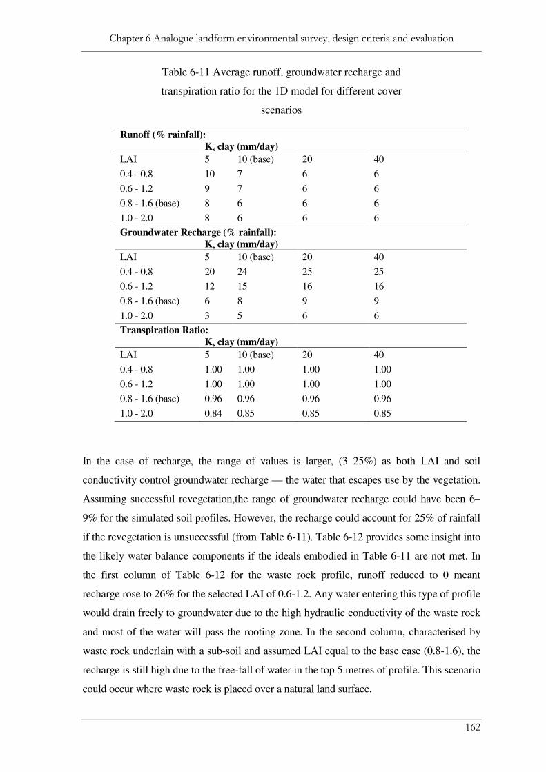
Chapter 6 Analogue landform environmental survey, design criteria and evaluation
162
Table 6-11 Average runoff, groundwater recharge and
transpiration ratio for the 1D model for different cover
scenarios
Runoff (% rainfall):
Ks clay (mm/day)
LAI 5 10 (base) 20 40
0.4 - 0.8 10 7 6 6
0.6 - 1.2 9 7 6 6
0.8 - 1.6 (base) 8 6 6 6
1.0 - 2.0 8 6 6 6
Groundwater Recharge (% rainfall):
Ks clay (mm/day)
LAI 5 10 (base) 20 40
0.4 - 0.8 20 24 25 25
0.6 - 1.2 12 15 16 16
0.8 - 1.6 (base) 6 8 9 9
1.0 - 2.0 3 5 6 6
Transpiration Ratio:
Ks clay (mm/day)
LAI 5 10 (base) 20 40
0.4 - 0.8 1.00 1.00 1.00 1.00
0.6 - 1.2 1.00 1.00 1.00 1.00
0.8 - 1.6 (base) 0.96 0.96 0.96 0.96
1.0 - 2.0 0.84 0.85 0.85 0.85
In the case of recharge, the range of values is larger, (3–25%) as both LAI and soil
conductivity control groundwater recharge — the water that escapes use by the vegetation.
Assuming successful revegetation,the range of groundwater recharge could have been 6–
9% for the simulated soil profiles. However, the recharge could account for 25% of rainfall
if the revegetation is unsuccessful (from Table 6-11). Table 6-12 provides some insight into
the likely water balance components if the ideals embodied in Table 6-11 are not met. In
the first column of Table 6-12 for the waste rock profile, runoff reduced to 0 meant
recharge rose to 26% for the selected LAI of 0.6-1.2. Any water entering this type of profile
would drain freely to groundwater due to the high hydraulic conductivity of the waste rock
and most of the water will pass the rooting zone. In the second column, characterised by
waste rock underlain with a sub-soil and assumed LAI equal to the base case (0.8-1.6), the
recharge is still high due to the free-fall of water in the top 5 metres of profile. This scenario
could occur where waste rock is placed over a natural land surface.

Chapter 6 Analogue landform environmental survey, design criteria and evaluation
163
Table 6-12 Average runoff, groundwater recharge and
transpiration ratio for the 1D model for the four cover
scenarios. All cases use base-case soil values unless
stated otherwise
LAI
1. All
primary
rock
2. Rock to
subsoil
3. No subsoil
4. Shallow
roots
5.
Weathered
rock
Runoff (% rainfall):
0.4 - 0.8 0 0 7 7 7
0.6 - 1.2 0 0 7 6 7
0.8 - 1.6 0 0 6 6 7
Groundwater Recharge (% rainfall):
0.4 - 0.8 32 32 24 24 23
0.6 - 1.2 26 24 15 17 14
0.8 - 1.6 22 8 10 13 7
Transpiration Ratio:
0.4 - 0.8 1.00 1.00 1.00 1.00 1.00
0.6 - 1.2 0.92 0.99 0.99 0.95 1.00
0.8 - 1.6 0.81 0.94 0.92 0.85 0.97
As shown in Table 6-12, column 3, which is characterised by subsoil in layers 8 to 12 with
highly conductive waste rock, did not affect runoff but increased the recharge under the
LAI of 0.8-1.6 to 10%. It also caused the transpiration ratio to drop from 0.94 to 0.92. This
case represents the situation where waste rock of considerable depth would cover the
tailings in the base of the backfilled pits.
The fourth column in Table 6-12, the shallow-rooting case, highlighted the sensitivity to a
poorly understood variable. Tree roots were assumed to reach 8–m in the base case (Table
6-4); in the shallower–rooting vegetation case they are assumed to reach 5–m, that is the
waste rock–subsoil interface. The reduced rooting depth has caused the base case LAI (0.8-
1.6) to have a transpiration ratio below the 0.9 water stress indicator. The reduced
transpiration ratio for the shallow rooting scenario implies that a lower LAI (0.6-1.2) is
likely and the recharge rate of 8% predicted in Table 6-11 could increase to 17% predicted
in Table 6-12.The last column in Table 6-12 presents the results of the weathering of the
waste rock and the reduction of its Ks from 24 000 mm.day-1
to 100 mm.day-1
. This large
change only reduced the rate of groundwater recharge from 8% for the base case in Table
Chapter 6 Analogue landform environmental survey, design criteria and evaluation
164
6-13 to 7% in Table 6-12. It takes only 12 days for a wetting front to pass through the
3 metres of the waste rock layer, and so, in terms of wet season time scales there is little
real difference between the two cases, in spite of the much lower conductivity. The water
holding capacity of the waste rock hasn’t been changed, only its conductivity.
The average runoff coefficient (9.6% of rainfall) was comparable to expected runoff
coefficients from the 1D modelling. However, because those areas with cover material had
a surface Ks of 50 mm.day-1
, while those without had a surface Ks of 1000 mm.day-1
, a
bimodal runoff response was simulated for extreme rainfall events. The daily simulated
runoff distributions on 2, 3 and 4 January 1997 in Figure 6-6 illustrate this bimodal
response. Rainfalls were 119 mm on the first day and 148 mm on the second. On 2 January
1997, runoff from the uncovered areas varied from 0 – 100 mm while for the covered areas
it was a uniform 59 mm. The amount of soil moisture store available in the A and B
Horizons controlled runoff on the uncovered areas, while the conductivity of the surface
soil in combination with its matrix potential controlled runoff from the covered area. So
uncovered (natural) and covered (waste rock) produced different runoff processes —
saturation excess controlled and infiltration excess controlled respectively.
The 3-D simulations indicated that there was no interflow within the covered areas, i.e.
seepage at the interface between the cover and the original soil-surface was completely
absent. This is because the downward flux at the interface between the cover and the soil
was less than the infiltration capacity of the underlying soil, and so, saturated conditions,
which are required to generate the interflow, don’t develop there. It is possible that a
situation could develop where such seepage takes place; but this would require either the
underlying soil to have a lower conductivity than the 2 mm.day-1
presently used, or the deep
groundwater system would rise to this level and create a saturation excess at the interface.
There was an average deep recharge rate of 9.4% of rainfall during the 13 years of the
simulation (146 mm.yr-1
or 1,900 mm in total). The present model is a closed system and
excess groundwater can only express itself as a groundwater rise. The simulated
groundwater depth for 16 May 2003 is depicted in Figure 6-7.

Chapter 6 Analogue landform environmental survey, design criteria and evaluation
Figure
Analogue landform environmental survey, design criteria and evaluation
Figure 6-6 Daily simulated runoff distributions on
2nd, 3rd and 4th January 1997
Analogue landform environmental survey, design criteria and evaluation
165

Chapter 6 Analogue landform environmental survey, design criteria and evaluation
Figure
The simulation started with a minimum groundwater depth of 20
rose by 2003 to be close to the surface
the simulations would produce groundwater seepage areas. If the post
groundwater discharge from the catchment can absorb the net recharge and negate the
simulated rises shown in Figure 6
information on the hydrogeology of the area is needed before this can be simulated.
6.3.3 Environmental surveys
6.3.3.1 Soil properties
The ranges in soil drainage status, gravel content, A horizon depth, A horizon textur
B horizon texture and depth to rock for each ecosystem type or class across the Georgetown
analogue area (defined from
Analogue landform environmental survey, design criteria and evaluation
Figure 6-7 Simulated groundwater depths for 16th
May 2003
The simulation started with a minimum groundwater depth of 20 metres and groundwater
rose by 2003 to be close to the surface over a large proportion of the catchment. Continuing
the simulations would produce groundwater seepage areas. If the post
groundwater discharge from the catchment can absorb the net recharge and negate the
simulated rises shown in Figure 6-7 then discharge will not occur. However, more
information on the hydrogeology of the area is needed before this can be simulated.
Environmental surveys
The ranges in soil drainage status, gravel content, A horizon depth, A horizon textur
B horizon texture and depth to rock for each ecosystem type or class across the Georgetown
analogue area (defined from Chapter 4) are depicted as box plots in Figure 6
Analogue landform environmental survey, design criteria and evaluation
166
metres and groundwater
over a large proportion of the catchment. Continuing
the simulations would produce groundwater seepage areas. If the post-rehabilitation
groundwater discharge from the catchment can absorb the net recharge and negate the
7 then discharge will not occur. However, more
information on the hydrogeology of the area is needed before this can be simulated.
The ranges in soil drainage status, gravel content, A horizon depth, A horizon texture,
B horizon texture and depth to rock for each ecosystem type or class across the Georgetown
in Figure 6-8.

Chapter 6 Analogue landform environmental survey, design criteria and evaluation
167
Figure 6-8 Range (boxes) and central tendency
(median line) of soil morphological properties
measured from 100 sites in the Georgetown analogue
area
The analogue area comprised very poor and poorly drained flats (ecosystem 4), poor to
imperfectly drained lower slopes (ecosystem 8), and imperfectly drained to well drained
crests and slopes on rises (ecosystems 3, 7 and 9). The depth to a root barrier, such as rock
or laterite, varied between 0.5 and 1.0 m for ecosystems formed on rocky substrates
(ecosystem classes 3, 6, 7, and 9) while soil depths in ecosystems with some colluvial or
alluvial influence (ecosystem classes 4, 8) were more variable. The soils were gravelly. The
soils on slopes and crests (ecosystems 3, 6, 7, 9) tended to be moderately gravelly to very
gravelly in the A horizon, where plant root activity is concentrated. Soils on flats and lower
slopes formed on colluvium and alluvium (ecosystems 4 and 8) were less gravelly. Surface
soil textures ranged from sand to sandy loam and subsoil textures ranged from sandy loam
to clay.

Chapter 6 Analogue landform environmental survey, design criteria and evaluation
168
Table 6-13 Summary statistics for soil physical and
hydraulic properties
Variable Unit N Minimum Median Maximum Range
gravel % 76 17.0 51.0 84.0 67.0
sand % 76 44.5 82.5 93.5 49.0
silt % 76 2.0 6.0 22.0 20.0
clay % 76 3.0 10.5 46.5 43.53
infiltration rate (dry) mm.min-
1
24 19.53 47.73 167.77 148.24
infiltration rate (wet) mm.min-
1
24 5.47 17.53 75.50 70.03
sub-soil permeability mm.min-
1
24 1.35 13.96 75.48 74.13
penetration resistance MPa 24 0.780 1.305 2.610 1.830
water retention @ -10kPa m3.
m-3
24 0.15 0.19 0.35 0.20
water retention @ -1500
kPa m
3.m
-3 24 0.03 0.0400
0
0.15000 0.12
plant available soil
water
mm.min-
1
24 110 145 320 210
density t.m-3
24 1.08 1.4800 1.9600 0.88
porosity % 24 26.23 44.18 59.10 32.87
aeration % 24 7.35 25.28 36.16 28.81
Soil profiles are gradational, characterized by gradual increase in clay content with depth
(Figure 6-9). The ranges of soil physical and hydraulic test statistics are presented in Table
6-13. Volumetric soil gravel contents ranged from 17 to 84%, which corroborates the field
morphological descriptions. The gravel fraction is relatively inert and do not contribute
significantly to water and nutrient retention or conduct flow.
In terms of soil fertility, the major nutrients, especially nitrogen and phosphorus, were
concentrated in the surface 0.2 metres of the soil profiles with maximum levels in the very
near surface 0 – 0.05 metres (Figure 6-10 a,b). However, potassium was more unevenly
distributed in the profiles and appeared to be superficially related to cation exchange
capacity (Figure 6-10 c,d).
The carbon profile in the soil was similar to distributions of nitrogen and phosphorus
(Figure 6-11 a). The profile distributions of the micronutrients iron (Fe) and manganese
(Mn) was also similar to the carbon profile (Figure 6-11 a,b), while copper (Cu) and zinc
(Zn) profiles were different from the carbon profile and are less closely associated with root
growth and nutrient cycling in the woodland vegetation.
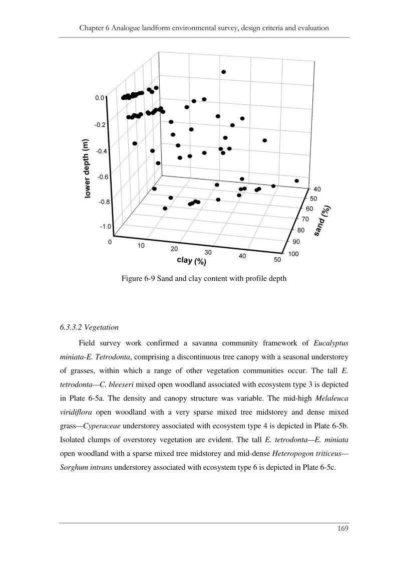
Chapter 6 Analogue landform environmental survey, design criteria and evaluation
169
Figure 6-9 Sand and clay content with profile depth
6.3.3.2 Vegetation
Field survey work confirmed a savanna community framework of Eucalyptus
miniata-E. Tetrodonta, comprising a discontinuous tree canopy with a seasonal understorey
of grasses, within which a range of other vegetation communities occur. The tall E.
tetrodonta—C. bleeseri mixed open woodland associated with ecosystem type 3 is depicted
in Plate 6-5a. The density and canopy structure was variable. The mid-high Melaleuca
viridiflora open woodland with a very sparse mixed tree midstorey and dense mixed
grass—Cyperaceae understorey associated with ecosystem type 4 is depicted in Plate 6-5b.
Isolated clumps of overstorey vegetation are evident. The tall E. tetrodonta—E. miniata
open woodland with a sparse mixed tree midstorey and mid-dense Heteropogon triticeus—
Sorghum intrans understorey associated with ecosystem type 6 is depicted in Plate 6-5c.

Chapter 6 Analogue landform environmental survey, design criteria and evaluation
170
Figure 6-10 Major nutrient and cation exchange
capacity profiles for analogue soils
There appeared to be differences in the density of recruiting overstorey species in the mid
and understorey. Tall E. tetrodonta—E. miniata—E. porrecta open forest with a sparse
mixed tree midstorey and mid-dense Sorghum intrans—Petalostigma quadriloculare
understorey associated with ecosystem type 7 is depicted in Plate 6-5d. Tall E. foelscheana
mixed open woodland with a sparse mixed tree midstorey and sparse Heteropogon
triticeus—Themeda triandra understorey associated with Ecosystem type 8 is depicted in
Plate 6-5e.
Mid-high E. tectifica—E. tetrodonta—E. confertiflora open woodland with a sparse mixed
tree midstorey and sparse Sorghum intrans—Eriachne spp. —Petalostigma quadriloculare
understorey associated with ecosystem type 9 is depicted in Plate 6-5f. A high level of
patchiness in canopy structure within as well as between ecosystems was evident from the
site photography.

Chapter 6 Analogue landform environmental survey, design criteria and evaluation
171
Figure 6-11 Total carbon and micronutrient profiles
for analogue soils

Chapter 6 Analogue landform environmental survey, design criteria and evaluation
172
The patchiness in plant community structure across ecosystem types is described in
Figure 6-12 a-f. Canopy cover varied from 60 to less than 20% while ground cover ranged
from 40 to 70%. Isolated clumps of melaleuca woodland in the wetland ecosystem type 4
produced a wide range of overstorey stem density. Stem densities in the other ecosystem
types (eucalypt woodlands) ranged between 200 and 400 stems per hectare. Woodland
height ranged from about 10 to 17 metres. Stem diameters ranged between 10 and 25
centimetres. Even though there were 2 to 7 species in the overstorey at most sites the
understorey contained many more species. Woodland ecosystems contained between 2 and
6 species in the overstorey (mostly eucalypts), between 2 and 11 in the midstorey and 11 to
40 understorey species. Species counts indicated that ecosystems 6 and 9 had the greatest
number of species on average, and ecosystem 4 (the melaleuca wetland) the lowest species
richness. However, the presence of relatively uncommon species in this ecosystem type
increased the Shannon-Weiner biodiversity index (Figure 6-12 i).
The framework species, their dominance (importance values) and their occurrence across
vegetation community (ecosystem) types are listed in Table 6-14. These species occurred at
more than one site in a particular ecosystem and across more than one ecosystem type. In
the overstorey, 8 species qualified as framework species. A further 14 species (including 3
overstorey species) qualified as framework species in the midstorey. An understorey
species qualified as framework species if it did not occur in other strata but was found in
more than one vegetation community. Ecosystem type 4 (Melaleuca grassland/sedge land)
was unique in structure.
The relative importance value (IV) in Table 6-14 identified Eucalyptus tetrodonta, E.
miniata and C. foelscheana to be the three most dominant framework overstorey species
and one that would fit well in rehabilitated woodland ecosystems at Ranger mine.
Cochlospermum fraseri, Acacia mimula, and Xanthostemon paradoxus were the three most
dominant in the midstorey stratum and the three most dominant understorey species were
Sorghum intrans, Petalostigma quadriloculare and Aristida holathera. Of the 126 species
recorded the presence of these 9 species occupied most of the available space across the
ecosystem range in the analogue area.

Chapter 6 Analogue landform environmental survey, design criteria and evaluation
173
(a) Ecosystem Type 3 (Sites 21, 73, 97): Tall Eucalyptus tetrodonta/E. bleeseri mixed open woodland with a sparse
mixed tree midstorey and mid-dense Sorghum intrans/Petalostigma quadriloculare understorey
(b Ecosystem Type 4 (Sites 27, 42, 36): Mid-high Melaleuca viridiflora open woodland with a very sparse mixed tree
midstorey and dense mixed grass/Cyperaceae understorey
(c) Ecosystem Type 6 (Sites 12, 56, 94): Tall Eucalyptus tetrodonta/E. miniata open woodland with a sparse mixed tree
midstorey and mid-dense Heteropogon triticeus/Sorghum intrans understorey
(d) Ecosystem Type 7 (Sites 8, 23, 65): Tall Eucalyptus tetrodonta/E. miniata/E. porrecta open forest with a sparse
mixed tree midstorey and mid-dense Sorghum intrans/Petalostigma quadriloculare understorey
(e) Ecosystem Type 8 (Sites 5, 64, 84): Tall Eucalyptus foelscheana/mixed open woodland with a sparse mixed tree
midstorey and sparse Heteropogon triticeus/Themeda triandra understorey
(f) Mid-high Eucalyptus tectifica/E. tetrodonta/E. confertiflora open woodland with a sparse mixed tree midstorey and
sparse Sorghum intrans/Eriachne sp./Petalostigma quadriloculare understorey
Plate 6-5 Ecosystem photos at vegetation plot survey
sites

Chapter 6 Analogue landform environmental survey, design criteria and evaluation
Figure
parameters each ecosystem typ
Analogue landform environmental survey, design criteria and evaluation
Figure 6-12 Ranges in overstorey and understorey
parameters each ecosystem type and grouped
woodland
Analogue landform environmental survey, design criteria and evaluation
174

Chapter 6 Analogue landform environmental survey, design criteria and evaluation
175
Table 6-14 Framework species in overstorey and
midstorey strata for each vegetation community type
Strata Family Species IV1
3 4 6 7 8 9
Overstorey Combretaceae Terminalia ferdinandiana 0.09 x x
(>8m) Myrtaceae Corymbia bleeseri 0.17 x
Corymbia foelscheana 0.68 x x
Corymbia latifolia 0.16 x
Eucalyptus miniata 0.75 x x x
Eucalyptus porrecta 0.34 x x
Eucalyptus tetrodonta 1.00 x x x
Xanthostemon paradoxus 0.37 x x x
Midstorey Bixaceae Cochlospermum fraseri 1.00 x x
(2-8m) Caesalpiniaceae Erythrophleum chlorostachys 0.07 x
Combretaceae Terminalia canescens 0.10 x x
Terminalia ferdinandiana 0.03 x x x
Lecythisaceae Planchonia careya 0.10 x x x
Mimosaceae Acacia mimula 0.63 x x x
Myrtaceae Eucalyptus confertiflora 0.04 x
Eucalyptus porrecta 0.07 x
Eucalyptus setosa 0.10 x
Eucalyptus tetrodonta 0.02 x
Melaleuca viridiflora 0.09 x
Syzygium suborbiculare 0.05 x
Xanthostemon paradoxus 0.26 x x x
Pandanaceae Pandanus spiralis 0.05 x
Proteaceae Grevillea decurrens 0.08 x
Hakea arborescens 0.04 x
Persoonia falcata 0.04 x 1 IV - Importance Values
6.4 Discussion and conclusions
6.4.1 Landform design
The landform design method presented here provides a clear geomorphic and
ecological context in the natural landscape, which facilitated communication of design
issues at different levels to a range of stakeholders. The description of ecosystem variation
across a natural analogue landscape that adequately represents the extent and grain size of
environmental processes in the mine landscape (from Chapter 4) also supports a capability
to extend the current topographic reconstruction approach (Toy and Chuse, 2005) to include
ecological objectives. The implications of the detailed environmental survey of soils,
vegetation and terrain properties in a selected natural analogue for landform design and
evaluation are discussed below.

Chapter 6 Analogue landform environmental survey, design criteria and evaluation
176
6.4.2 Environmental evaluation
Gully erosion, plant available water store and groundwater recharge were identified
from landscape evolution and hydro-ecological modelling of a first pass landform design
that was based on the ranges in slope, relief and catchment area observed in an analogue
landscape. These issues can be addressed in the next iteration of the design. In some
respects, the landform evolution and hydro-ecological modelling methods also need further
development before reliable quantitative assessments can be made. Parameterisation of the
SIBERIA landform evolution model (Lowry et al., 2006) did not have the flexibility to
allow variation in cover properties that affect runoff. Also, gully initiation in convex
shoulder slopes of the landform may to some extent be artefacts of the D8 flow routing
algorithm used in the SIBERIA model. A number of enhancements to the model that
address some of these issues have been made (Hancock et al., 2008). However, different
modelling approach that accurately represents soil forming processes causing temporal
changes in soil hydraulic properties, chemical fertility and plant available water could be
considered. Mechanistic soil formation models (Minasny et al., 2008) may offer some
insights in this respect.
The hydro-ecological simulations highlighted that recharge rates depended on the density of
vegetation cover and that the vegetation density depended on the soil profile or landform
cover, particularly with respect to the rooting depth, water retention and the downward flux
of water. Due to variations in rainfall, both recharge and drought are episodic with low
rainfall periods having no significant recharge and high rainfall periods averaging 17%
rainfall recharge. Consequently a simulation approach, with support from monitored natural
and reconstructed catchments, will be needed to assess the hydrological performance of the
mine rehabilitation.
The mechanics of the processes controlling water balance components ET, stream flow
generation and groundwater recharge, will determine whether the mine rehabilitation will
restore the pre-mine water balance in the upper layers, or whether it will move towards a
state with a different total ET and thereby different rates of stream flow and groundwater
recharge to that of the natural landscape. Water balance simulation implied the long-term
average recharge for the rehabilitated mine area will be something like 8 to 9% of rainfall
for the areas overlaying a subsoil and 10% of rainfall for the areas overlaying the pits. In
the natural situation, excess water vents from the system via stream flow, which accounts

Chapter 6 Analogue landform environmental survey, design criteria and evaluation
177
for more than 20% of the water budget compared with 34% for Howard River while
estimated ET was 1 110 mm.yr-1 for Howard River (Cook et al., 1998) and 1 240 mm.yr-1
for Corridor Creek. This assumes that the revegetation reaches a density similar to that of
the surrounding native areas.
Runoff generation processes in areas with, and without, waste rock cover material behave
differently. This is consistent with studies of mine and natural catchment hydrology in the
short term {Duggan, 1991 #730}. Over the longer term (approximately 50 years) runoff
rates from mine landforms may trend towards that from the natural landscape as vegetation
becomes established and rudimentary soils form {Moliere, 2002 #932}. However, initially
the covered areas generate runoff during intense rainfall events via an infiltration excess
process, while the uncovered areas have a combination of saturation excess and interflow
processes. Also there appears to be no interflow from the covered areas at the cover–soil
interface. The groundwater system must be able to absorb a net recharge rate of around
9.4% of rainfall to prevent groundwater rise. The rate of groundwater rise still needs to be
determined.
6.4.3 Environmental surveys
The current work has broadened the scope of existing analogue studies for Ranger
mine (Brennan, 2005), which documented well drained woodland sites across the region.
The analogue design methods support a range of revegetation outcomes that are integrated
with hill slope topography and soil pattern to extend topographic reconstruction methods
(Toy and Chuse, 2005) so as to support ecosystem reconstruction in the mine landscape
(Nicolau, 2003). This development has practical implications that could improve the
success of mine rehabilitation using natural analogues. For instance at Nabarlek mine site
nearby to Ranger mine, the topographically reconstructed mine landscape failed to meet the
objective to establish uniform eucalypt woodland (Klessa, 2000) because the effects of hill
slope hydrology on environmental pattern in the rehabilitated landscape were not resolved.
The soils in the natural analogue area at Ranger are rocky, moderately deep and are
gradational in texture profile. These properties are similar to the waste rock cover materials
reported on in Chapter 5. However, organic matter associated with enhanced levels of
macro and micronutrients has accumulated near the land surface in the native soils that
could take time to develop in the revegetated mine soils. This pattern has been observed

Chapter 6 Analogue landform environmental survey, design criteria and evaluation
178
elsewhere in tropical and temperate deep weathered landscapes (Parrotta and Knowles,
2001; Schwenke et al., 2000b). In noting this, soil organic matter accumulation is a key
component in assessing functional integrity of ecosystems in general (Ludwig et al., 2004)
and rehabilitated mine soils in particular (Koch and Hobbs, 2007). A solution to this slow
accumulation of organic matter is by carefully conserving and using natural topsoil in
rehabilitation to enhance the process (Bell, 2001; Parrotta and Knowles, 2001). At Ranger
mine, mine scheduling and weed problems meant that topsoil was not conserved and
different measures will be needed to restore soil fertility and ensure successful revegetation
and rapid development of surface organic carbon content – the key to nutrient cycling
across a range of low fertility soils.
The structure of natural plant communities was patchy and this patchiness increased in
areas that were poorly or imperfectly drained. The number of species also declined as
drainage was impaired from hill slope to valley flat. Consequently, revegetation objectives
that do not account for the patchiness induced by hill slope environmental variation are
unlikely to be achievable and terrain factors that affect drainage could be expected to
influence revegetation outcomes.
6.4.4 Further work
Research into the eco-hydrology of natural and reconstructed landscapes to support
ecosystem restoration tasks would improve the methodology presented here. Site based
measurements of tree canopy characteristics, water use by vegetation and catchment water
balance have not been presented and are essential. Further investigations are needed to
support accurate hydrological assessment of the mine rehabilitation. The need for a paired
catchment study of a constructed landform and a natural analogue catchment was raised in
Chapter 5. This study could be designed to address the significant gaps in knowledge of
hydrological processes. However, water retention in the root zone, sub-soil hydraulic
conductivity and successful revegetation strategies supporting high canopy leaf areas will
be key factors in restoring the landscape. Assuming that all of these factors can be
addressed, then the landform design and the vegetation survey results presented in this
chapter are a basis for predicting the distribution of common and abundant overstorey, or
framework species, in the revegetated mine landscape. This is the objective of the next
chapter.

Chapter 6 Analogue landform environmental survey, design criteria and evaluation
179
A framework of common and abundant species is identified. In the overstorey, 8 species
and in the mid-storey 11 additional species qualified as framework species, while 9
overstorey, midstorey and ground cover species occupied most of the available
environmental space. One additional species, Melaleuca viridiflora, had a limited range —
dominating the overstorey and mid-storey in less biodiverse low lying, poorly drained
areas. Understanding the way that landform design affects the distributions of these species
will underpin successful revegetation for the case study site. In Chapter 4, terrain was
identified as an important factor affecting species distributions. Quantitative species
distribution models based on the vegetation survey data from Chapter 4, Chapter 6 and
regional vegetation surveys are developed in Chapter 7.

Chapter 7 Ecological modelling for landscape reconstruction
180
Chapter 7 Ecological modelling for landscape reconstruction
7.1 Introduction
7.1.1 Background
Landscape restoration following opencast mining requires a site-specific
understanding of the biophysical factors that determine environmental patterns in natural
landscapes. In the first stage, quantitative methods to select and analyse natural analogue
landscapes was presented in Chapter 4. The broad range of ecosystems (represented by
vegetation type) in selected natural analogue landscapes that were similar, from
environmental terrain analysis, to a mine area were described. In the second stage presented
in Chapter 6, the biophysical environment was described from grid and stratified
environmental surveys in the selected, analogue landscape to support an ecological
landform design evaluation process. Common and abundant plant species that provided an
ecological framework in the analogue landscape were identified and basic data on species
distribution at 200-m resolution was obtained. Chapter 7 uses this survey support to model
the distribution of common and abundant woodland species and biodiversity in the
landform design to test the analogue approach.
Elsewhere, the biodiversity surveys that support environmental restoration of landscapes
have focussed on regional conservation values (Johnson and Miyanishi, 2008; Tischew and
Kirmer, 2007), substrate and geochemical properties (Riley and Rich, 1998; Suksi et al.,
1996; Uren, 1992), and regional land resources mapping (Brennan, 2005; East et al., 1994;
Hobbs and McIntyre, 2005). The need to integrate landscape ecological science into
restoration practice to achieve success has been recognised (Bradshaw, 1997; Holl et al.,
2003; Temperton, 2007). Species distribution modelling is a means of achieving this
integration.
The topographic variables derived from DEMs (Chapter 4) are used as environmental
predictors in almost every published example of predictive mapping of terrestrial vegetation
(Austin, 2007; Guisan and Zimmermann, 2000). However, the reliability that can be
achieved from species distribution modelling depends on the combined effect of the
ecological model to be tested, a data model and a statistical modelling approach (Austin,

Chapter 7 Ecological modelling for landscape reconstruction
181
2002b). A brief introduction to these three aspects affecting reliable prediction of species
distribution follows.
7.1.2 Ecological modelling
The data models and methods used for conservation reserve planning are focused
predominantly on rare and endangered species and have a regional context (Austin, 2002b;
Ferrier and Guisan, 2006; Lehmann et al., 2002b). However, the data models and methods
used in mine landscape reconstruction can be applied to common and abundant species that
provide the ecological framework of locally extensive ecosystems in natural analogue
landscapes. Many studies have modelled the influence of landscape factors on the
composition and structure of plant communities (Austin, 1987; Austin et al., 1984; Austin
et al., 1983; Coops and Catling, 2002; Woinarski and Fisher, 2003; Woinarski et al., 2005)
and confirm the notion that plant communities change continuously along environment
gradients.
There is a strong argument for modelling individual species distributions first and then
assembling the predictions to account for vegetation community dynamics (Guisan et al.,
2006). The most robust approach is to predict the distribution of individual species rather
than plant communities (Ferrier and Guisan, 2006; Guisan and Thuiller, 2005; Guisan and
Zimmermann, 2000; Lehmann et al., 2003). Ecosystem dynamics are then represented in
the autocorrelated component. Although, significant autocorrelation can also identify that
the theoretical ecological framework needs to be reassessed (Austin, 2007).
The strength of modelling individual species distributions is that it does not assume
community structure to be stable over time (Ferrier and Guisan, 2006). Although
equilibrium between the environment and observed species patterns is still assumed,
modelling individual species rather than species assemblages and classifying their
superimposed distributions afterwards is more logical than fitting a priori community
classifications (Ferrier and Guisan, 2006; Guisan and Thuiller, 2005).
7.1.3 Statistical method
Statistical models that account for non-linearity in species presence–absence
responses to environment, such as generalised additive models, or GAMs (Hastie and
Tibshirani, 1990), are the preferred method for species distribution modelling (Austin,

Chapter 7 Ecological modelling for landscape reconstruction
182
2007; Austin, 2002b; Guisan et al., 2002; Guisan et al., 2006; Guisan and Thuiller, 2005).
Generalised additive models (GAMs) allow almost any response curve to be fitted. This is
an important advantage since species rarely present pure bell-shaped or linear response
curves along environmental gradients (Guisan and Harrell, 2000).
Parsimonious variable selection for data models is an important issue to minimise error and
uncertainty (Barry and Elith, 2006; Fielding and Bell, 1997). Maggini (2006) tested a range
of variable selection methods and found that a cross validation approach (Stone, 1977)
provided the best compromise between model performance and parsimony or model
stability. For presence–absence data, area under the curve (AUC) methods, considered to be
the current best practice for assessing model success (Austin, 2007), have been used
extensively in species distribution models (SDMs) (Elith et al., 2006).
Another issue is the problem of autocorrelation. Incorporation of the autocorrelation of
model residuals into predictive models may minimise model uncertainty (Maggini et al.,
2006; Malanson et al., 1992), although, optimal parameterisation and sampling can be
obscured when autocorrelation is included (Austin, 2002b). Lehmann (2003) offers a
solution to this approach using GAM implemented in S+Plus2000 in the GRASP module
(Generalised Regression and Simulation Package). A wide range of GRASP applications
have been published spanning different groups and ecosystems, including terrestrial
vegetation species (Cawsey et al., 2002; Clarkson et al., 2004; Lehmann et al., 2002a) and
mapping of plant communities (Ferrier and Guisan, 2006).
7.1.4 Data model
Statistical modelling is sensitive to the quality and range of the survey data (Barry
and Elith, 2006; Legendre et al., 2002; Van Niel and Austin, 2007). Restricted
environmental sampling reduces the combinations of environmental variables under which
statistical models of environmental correlation are calibrated and this limits the extent of
their application (Thuiller et al., 2004). However, using species presence–absence data for
species distribution modelling rather than abundance data (Cushman and McGarigal, 2004;
Guisan and Zimmermann, 2000) is cheaper, quicker and does not appear to degrade results
(Margules and Austin, 1991). The number and range of observations is more critical to the
reliability of species distribution models than using abundance data.

Chapter 7 Ecological modelling for landscape reconstruction
183
The survey design needs to resolve local environmental pattern (Austin and Heyligers,
1989; Edwards et al., 2006) that are often scale dependant. Grid survey designs have been
applied to targeted natural landscapes to resolve observed hill slope patterns affecting the
environmental range (Ben Wu and Archer, 2005). This approach does not presume that
ecological complexity, which affects short range variation, is fully understood. Extensive
ecosystems would be over–represented and ecosystems with limited extent would have
fewer observations. Using grid spacings less than the natural hillslope lengths would
account for the effects of hillslope environmental process (erosion, sedimentation and water
distribution) that drive diversity.
One hundred sites appear to be a minimum to quantify species distribution (Austin, 2007;
Maggini et al., 2006; Pierce et al., 1993; Stockwell and Peterson, 2002). Environmental
complexity, particularly anisotropic spatial autocorrelated variation, may increase the
minimum number of survey sites to 250 (Webster and Oliver, 2001). Also, species
prevalence (frequency of species’ occurrences in the data set) can shift prediction errors
from omission (under prediction of true presences) to commission (over prediction) with
the best compromise occurring at about 0.5 (Liu et al., 2005). Other authors have suggested
the use of weighting absences to adjust sample prevalence towards this value to reduce
modelling errors (Lehmann et al., 2003; Maggini et al., 2006). The number of sample sites
needed to quantify species distribution depends on the abundance (prevalence) of the
species concerned and environmental complexity.
Statistical models need to be calibrated and validated. Calibration and validation of models
using independent data sets is ideal (Fielding and Bell, 1997; Guisan and Harrell, 2000) but
it can be difficult to justify excluding data to calibrate the model. An alternative cross-
validation, or bootstrapping, approach tends to give the upper boundary of error
probabilities (Fielding and Bell, 1997; Maggini et al., 2006). Consequently, K-fold cross-
validation (Franklin et al., 2000) and bootstrapping methods (Guisan and Harrell, 2000)
offer a compromise that allow model stability to be assessed without losing information
during calibration.
7.1.5 Objectives
The primary objective of this chapter was to develop statistical models for the
distributions of framework species in the context of an open-cast mine restoration project

Chapter 7 Ecological modelling for landscape reconstruction
184
and apply these models to predict revegetation outcomes in a mine landform design.
Supplementary objectives were to: (i) assess the effect on measured species response of
using presence-absence or abundance data and sample size; (ii) investigate aspects of the
predictor variables including geographic range and the significance of autocorrelation. The
work focuses on the Ranger uranium mine case study site.
7.2 Methods
The grid environmental survey was made of the 500 hectare Georgetown analogue
area adjacent to the mine (Chapter 6) and provided the core dataset for the GAM modelling
of species distribution presented in this chapter. This area contained the environmental
range found on rock substrates recorded over a much larger area (79 km2, see Chapter 4).
The reconnaissance survey data that was collected from two analogue areas (Georgetown
and 7J) in Chapter 4 and information from a regional natural analogue survey of well
drained woodland habitats (Brennan, 2005) has been introduced to assess the effect of
increasing survey support with regional information to measure trends in species response
to environment. Initially, multivariate analytical methods were used to test the null
hypothesis that species distribution was unrelated to environmental gradients for presence-
absence and abundance date. Finally, univariate (GAM) models of framework woodland
species are developed and applied to a landscape that incorporates the draft Ranger mine
landform design that was presented in Chapter 6.
7.2.1 Field survey data
The field survey data included: (i) 101 survey sites located 200 hundred metres apart
in a square grid survey over the Georgetown analogue landform (500 hectares) on the
Ranger mine lease (Chapter 6); (ii) 32 sites in a environmentally stratified sampling design
over the 79 km2 Ranger lease area (79 km
2, Chapter 4); (iii) 28 detailed plot survey sites
over the East Arnhem Land (10 000 km2) from Brennan (2005). The locations of the sites
on the Ranger lease area are shown in Figure 7-1. The quantitative vegetation survey data
of species abundance and community structure at 18 plot survey sites were presented in
Chapter 6 for the Georgetown analogue area. This data is now supplemented with 10
vegetation survey sites over the Alligator Rivers region comprising Kakadu National Park
and East Arnhem Land and covering 10 000 km2. The common and abundant species

Chapter 7 Ecological modelling for landscape reconstruction
185
across the environmental range in the Georgetown analogue area listed in Table 7-1 were
selected for species distribution modelling.
Table 7-1 Selected common and abundant species in
the overstorey and midstorey across analogue areas
Strata ID Species
Overstorey 1 Eucalyptus tetrodonta
(>8m) 2 Eucalyptus miniata
3 Corymbia bleeseri
4 Corymbia foelscheana
5 Corymbia latifolia
6 Corymbia porrecta
7 Corymbia setosa
8 Eucalyptus tectifica
9 Xanthostemon paradoxus
Midstorey 10 Acacia mimula
(2-8m) 11 Melaleuca viridiflora
12 Erythrophleum chlorostachys
13 Petalostigma pubescens
14 Pandanus spiralis
These are ‘framework’ species (identified in Chapter 6) and their establishment is a key
concern in the revegetation strategy for Ranger Mine. Although the revegetation strategy
excluded acacias, Acacia mimula is included in the analysis because it is ubiquitous in the
midstorey layer and provides habitat for small mammals (Woinarski et al., 1999a;
Woinarski et al., 1999b). Also, although Melaleuca viridiflora was identified as a midstorey
species in Chapter 6, it is the dominant overstorey species in Melaleuca woodland
communities.
7.2.2 Terrain analysis
The factors and environmental correlates that influence environmental variation
across the study area are summarised in Table 7-2. Landscape or terrain variables derived in
Chapter 4 from a digital elevation model (DEM) were used as predictors; all other variables
were treated as covariates.

Chapter 7 Ecological modelling for landscape reconstruction
186
Figure 7-1 Sites in analogue areas on the Ranger lease
surveyed for species presence-absence

Chapter 7 Ecological modelling for landscape reconstruction
187
Table 7-2 Environmental factors in the vegetation
model
Variable influencing species
distribution
Significance and
interpretation
Potential environmental
correlates
climate
temperature nature and rate of biological activity
climate surfaces
wetness nature and rate of biological activity
climate surfaces and terrain attributes
parent material
substrate influences nutrient levels and drainage
geophysical remote sensing
erosion and deposition influences water and nutrient supply
terrain attributes and geophysical remote sensing
time
age of land surface older relief may not reflect contemporary environmental conditions
empirical correlations with terrain attributes
biomechanical impact
termites, ants local scale disturbance (termites, ants, etc.) may control nutrient and water supply
no effective predictors
disturbance
fire fire frequency and intensity affect biodiversity
fire frequency mapping late in the dry season when intensive fire impacts occur
endogenous vectors
soil morphology affects local conditions
inherited soil profile features may impose limitations
realised plant niche differs from idealised distribution
model species individually
The topographic variables used to predict species distribution are listed in Table 7-3. The
environmental covariates that were used are listed in Table 7-4. Continuous variation in the
mineral properties of parent materials was assessed using airborne gamma radiometric
mapping from NT Geological Survey. The radiometric data show a strong U signal
associated with outcropping schists particularly in the Arnhem Plateau and Pine Creek
regions with clear anomalies at Ranger and the northern extent of the Arnhem Plateau
region. The thorium signal is associated with exposed petroferric horizons and strong K
signal associated with alluvial clays (Wilford, 2006) that are extensive in floodplains of the
Darwin Coastal region.

Chapter 7 Ecological modelling for landscape reconstruction
188
The distribution of late dry season fires was also used as covariate in the statistical analysis
and was mapped from monthly fire scar mapping (NOAH AVHR imagery). The resolution
of the imagery (1 km2) is coarse relative to the DEM (50-m).
Table 7-3 Topographic variables used for
environmental prediction
ID Environmental variable Description Source
Primary topographic attributes1
1 elevation elevation above sea level DEM
2 slope measured in percent TAPESG
3 relief absolute range in elevation within 600 m circle
TAPESG
4 aspect N, NE, E, SE, S, SW, W, NW, level (zero slope)
TAPESG
5 plan curvature rate of change of aspect, generated using a 3x3 window
TAPESG
6 profile curvature rate of change of slope generated using a 3x3 window
TAPESG
Secondary topographic attributes1
7 wetness index static wetness index describes the spatial distribution and extent of zones of saturation
TAPESG
8 slope length index (LS) sediment transport capacity index equivalent to the length-slope factor in the Revised Universal Soil Loss Equation
TAPESG
9 stream power index measure of erosive power that predicts net erosion in convex areas and net deposition in concave areas
TAPESG
10 upslope flow path length maximum distance of flow to a point
TAPESG
11 contributing area upslope area above a point TAPESG
12 dispersal area dispersal area below a point TAPESG
1(Wilson and Gallant, 2000b).
7.2.3 Multivariate analysis
Multivariate hybrid gradient analysis methods detrended correspondence analysis
(DCA) and canonical correspondence analysis (CCA) methods in the CANOCO VERSION
4.2 statistical package (ter Braak and Smilauer, 2002) were used to identify environmental
trends in species abundance and presence-absence data. The multivariate analysis used a
forward selection procedure and a Monte Carlo permutation to test variable significance.
Two Monte Carlo permutation tests were performed to measure statistical significance

Chapter 7 Ecological modelling for landscape reconstruction
189
using an F-test (0.05 probability level) of the first and combined canonical ordination axes
(ter Braak and Smilauer, 2002). This tested the null hypothesis that species response was
unrelated to environmental gradients.
Table 7-4 Environmental covariates
ID Environmental
variable
Description Source or reference
Parent material
13 Gamma-K K band response from gamma radiometric mapping
NT Geological Survey :Kakadu II 1982, Alligator River 1976, Koolpinyah 1974 radiometric grids (150 m line spacing, www.minerals.nt.gov.au/ntgs)
14 Gamma-Th Th band response from gamma radiometric mapping
As above
15 Gamma-U U band response from gamma radiometric mapping
As above
Climate
16 Prescott Index Ratio of annual rainfall to annual evapotranspiration
Australian climate surfaces (www.bom.gov.au)
17 Fire frequency Years in 10 frequency of late dry season fires
NT Bushfires Council fire scar mapping from monthly NOAA imagery
Biodiversity
18 Bioregionalisation Sub-region classification National Bioregionalisation mapping (Thackway and Cresswell, 1995)
Soil morphology
19 A horizon thickness class
Field survey
20 A horizon gravel class Field survey
21 A horizon texture class Field survey
22 B horizon texture class Field survey
23 Depth to rock Field survey
24 Drainage class Field survey
7.2.4 Modelling experiments
The univariate methods were used to conduct a number of modelling experiments to
test the effects of parameterisation and data model and to develop species distribution
models (SDMs) for framework species. The univariate GAM models were calibrated using
the GRASP Version.3.2 package (Lehmann et al., 2003) for S-PLUS Version 2000
(Insightful Corp., Seattle, WA, USA). The response variables were the common and

Chapter 7 Ecological modelling for landscape reconstruction
190
abundant woodland species defined as binary variables, and N2 species richness (number of
species) defined as a continuous variable with a Gaussian distribution. In using GAM for
species presence-absence data, a quasi-binomial model was chosen; whereas for N2 species
richness, a quasi-Poisson model was most appropriate (Lehmann et al., 2002b). In both
cases, a stepwise ‘cross-selection’ method also termed as CROSS, was used to select the
predictors. With CROSS a CVROC (cross–validated receiving operator characteristic) was
calculated at each step of the selection procedure. The receiver operating characteristic
(ROC) was used to test goodness of fit for the binomial model (Fielding and Bell, 1997).
The selection stops when no more predictors can be added or removed according to a
Bayesian information criterion (BIC), the most selective criterion available. CROSS then
selects the model showing the highest value of CVROC.
Pearce et al. (2001) recommended using 2 degrees of freedom (df) in the GAM function for
presence–absence vegetation survey data. However, using the default setting in GRASP (4
degrees of freedom) produced a more valid model (ROC 0.848; CROC 0.684). This result
was with the default cross–validation selection direction, ‘backwards’. Changing the search
direction to ‘both’ caused model instability (ROC 0.93; CROC 0.679). The modelling
experiments carried out on the analogue data are listed in Table 7-5.
Modelling alternatives and the effect of varying the data model to increase support (number
of sites) were tested. The first experiment (E0) involved testing the differences in
environmental correlation between presence-absence data (143 sites) and abundance data
(28 sites) with the aim of identifying trends and modelling limitations with these data sets.
The set of 12 explanatory environmental variables and their relationships with the presence-
–absence of 60 species recorded at 143 sites were analysed based on a unimodal model in
CCA. Analysis for the effect of covariates on gradient lengths was done before and after the
inclusion of bioregional, climatic, parent material, fire frequency and soil morphological
variation. All subsequent experiments (E1-E7) calibrated univariate GAM models.
The second group of experiments (E1-E4) tested the effect of weighting absences and
removing absences outside the community range along the key environmental gradients,
recommended practices in pre-processing presence-absence data in regional biodiversity
modelling (Austin and Nicholls, 1997; Leathwick, 1998). E1 baseline models were
developed using presence-absence data for 101 sites in the Georgetown analogue area with

Chapter 7 Ecological modelling for landscape reconstruction
191
no weighting of absences or masking the environmental range to remove strings of
absences.
Table 7-5 Modelling experiments conducted on
analogue site data
Experiments Description
Environmental correlation
E0 Multivariate environmental model (presence-absence response) ~ [topography], [climate, geology, fire, soils]
Multivariate environmental model (abundance response) ~ [topography], [climate, geology, fire, soils]
Univariate models
E1 (baseline) Univariate environmental models ~ topography; Georgetown sites
Weights (compared with E1)
E2 Univariate environmental models ~ topography; Georgetown sites; weighted absences
Support size (compared with E2)
E3 Univariate environmental models ~ topography; with weighted absences; 101 Georgetown grid sites + 32 Ranger Project Area sites = 133 sites
E4 Univariate environmental models ~ topography; with weighted absences; 101 Georgetown sites + 32 Ranger Project Area sites + 10 regional analogue sites = 143 sites
Spatial autocorrelation (compared with E2)
E5 Univariate environmental models ~ topography + trend (tested); with weighted absences; 101 Georgetown sites + 32 Ranger Project Area sites + 10 regional analogue sites = 143 sites
E6 Univariate environmental models ~ topography + εenv ; with weighted absences; 101 Georgetown sites Spatial model: εenv ~ IK*
E7 Univariate environmental models ~ topography + IK* (tested); with weighted absences; 101 Georgetown sites
Experiment E2 tested the effect of weighting absences and masking environmental range.
An overall prevalence of 0.5 was obtained by giving the presences a weight of 1, and the
absences a weight defined by the ratio of the number of presences on the number of
absences. A model was then fitted using these weights. Results were compared with E1
baseline models. Species absences at environmental extremities were masked to create
environmental envelopes. Experiment E3 augmented the survey support to one hundred and
thirty three sites with thirty two sites in the Ranger project area (Chapter 4). Experiment E4

Chapter 7 Ecological modelling for landscape reconstruction
192
further augmented the survey design with 10 sites remote from the Ranger mine from a
regional analogue survey (Brennan, 2005).
The third group of experiments (E5-E7) tested the effect of spatial autocorrelation. In
experiment E5, first-order spatial autocorrelation was incorporated into the models by
adding a trend predictor. A first order trend surface was fitted using all 143 sites and added
to the GAM model. Experiment E6 investigated second-order spatial models based on the
101 sites in the Georgetown analogue area. GAM analysis was performed and indicator
kriged (IK) estimates of local auto correlation were calculated. The IK term of spatial
autocorrelation was added to the list of predictors, which was tested using cross-validation
selection criteria in GRASP. Experiment E7 investigated the local autocorrelation using an
autoregression term (Maggini et al., 2006). This term was regressed against the residuals of
the E1 model to account for the residual spatial autocorrelation still present after
environmental correlation. The results were compared with the E1 baseline models using
the Wilcoxon signed-rank test, a distribution-free test of pairwise difference measure. The
final experiment (E7) tested the effect of extending the Georgetown analogue data set with
the reconnaissance survey data of the Ranger project area (Chapter 4) making 133 sites.
7.2.5 Validation
Observed response values were plotted against predicted, by correlation (COR) and
also by fivefold cross-validation of the model, to evaluate GAM models. The area under the
ROC function (AUC) provides a single measure of overall accuracy independent of a
particular threshold. An AUC value of 0.5 indicates the scores for two groups do not differ,
while a score of 1.0 indicates no overlap in the distributions of the group scores. A value of
0.8 for the AUC means that for 80% of the time a random selection from the positive group
would have a score greater than a random selection from the negative class. Cross-
validation performance (CVROC) on randomly selected sub-samples of the data indicates
instability in the model. The goodness of fit of the Poisson model of N2 species richness
was assessed from correlation between actual and predicted values.
The effect of varying modelling options in GRASP on model performance was tested for
Melaleuca viridiflora to optimise the setup before running the modelling experiments.
Melaleuca viridiflora had a relatively low prevalence in the survey, 0.3 compared with
Eucalyptus tetrodonta 0.69, while its dominance is definitive for a woodland community

Chapter 7 Ecological modelling for landscape reconstruction
193
type (Melaleuca woodland). Wilcoxon signed-rank tests were used to compare validation
statistics between pairs of modelling experiments. This test, which does not assume any
particular distribution, can be applied as a one-way test of competing results.
Spatial predictions were built in S-PLUS using optimised GAM models for the 20 km2 (50-
m grid resolution) that covered the Ranger mine, including the final landform surrounded
by undulating rises. The grid of prediction variables was generated in ArcGIS version. 9.2.
The predicted species distributions were exported back to ArcGIS for display.
7.3 Results
7.3.1 Multivariate environmental response
Gradients longer than 4.0 in Table 7-6 for the first and second ordination axes
indicated environmental trends for which unimodal methods (such as DCA and CCA) are
likely to be appropriate (ter Braak, 1988). Transforming and detrending the species data did
not alter or improve the analytical results. The first two extracted CCA axes provided the
best species–environment correlations and interpretations and the species-environment
correlation decreased only very slightly when covariates (soils, fire frequency, climate,
parent material) were included in the analysis (partial CCA in Table 7-6). Apparently,
covariates (non-terrain variables) were not significant factors in explaining species-
environment relationships.
The unimodal models adequately described the environmental gradients for Corymbia
foelscheana (CORYFOEL), Eucalyptus tectifica (EUCATECT) and Corymbia latifolia
(CORYLATI) (Figure 7-2). The open ended, more linear models for Eucalyptus tetrodonta
(EUCATETR), Eucalyptus miniata (EUCAMINI), Corymbia bleeseri (CORYBLEE),
Corymbia setosa (CORYSETO), Xanthostemon paradoxus (XANTPARA) and Corymbia
porrecta (CORYPORR) indicated that their environmental ranges were only partially
sampled in this data set.
The combined canonical axes for CCA and partial CCA (Table 7-7) were significant (P =
0.05) meaning that the null hypothesis, based on the premise that species variation was
unrelated to environmental gradients, was dismissed for the 148 samples of species
presence–absence. However, the null hypothesis was accepted for the smaller species
abundance sample (28 samples) based on the P-value shown in Table 7-7, even though the

Chapter 7 Ecological modelling for landscape reconstruction
194
environmental trends in relation to the first and second ordination axes were investigated
further.
Figure 7-2 Species response (GAM) to 1st Ordination
axis
The next objective was to identify significant environmental predictors of species
distributions. Five environmental variables out of 12 were significant predictors (P<0.05,
Table 7-8) for species presence-absence.
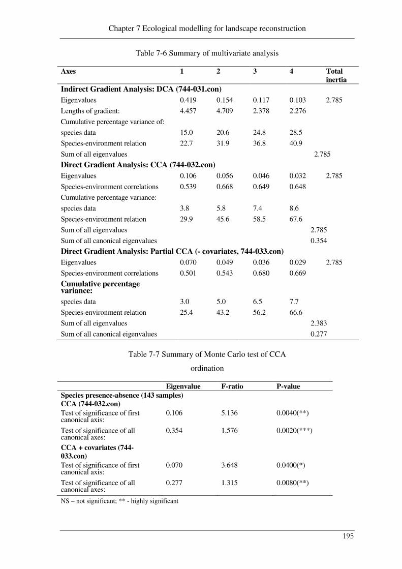
Chapter 7 Ecological modelling for landscape reconstruction
195
Table 7-6 Summary of multivariate analysis
Axes 1 2 3 4 Total
inertia
Indirect Gradient Analysis: DCA (744-031.con)
Eigenvalues 0.419 0.154 0.117 0.103 2.785
Lengths of gradient: 4.457 4.709 2.378 2.276
Cumulative percentage variance of:
species data 15.0 20.6 24.8 28.5
Species-environment relation 22.7 31.9 36.8 40.9
Sum of all eigenvalues 2.785
Direct Gradient Analysis: CCA (744-032.con)
Eigenvalues 0.106 0.056 0.046 0.032 2.785
Species-environment correlations 0.539 0.668 0.649 0.648
Cumulative percentage variance:
species data 3.8 5.8 7.4 8.6
Species-environment relation 29.9 45.6 58.5 67.6
Sum of all eigenvalues 2.785
Sum of all canonical eigenvalues 0.354
Direct Gradient Analysis: Partial CCA (- covariates, 744-033.con)
Eigenvalues 0.070 0.049 0.036 0.029 2.785
Species-environment correlations 0.501 0.543 0.680 0.669
Cumulative percentage variance:
species data 3.0 5.0 6.5 7.7
Species-environment relation 25.4 43.2 56.2 66.6
Sum of all eigenvalues 2.383
Sum of all canonical eigenvalues 0.277
Table 7-7 Summary of Monte Carlo test of CCA
ordination
Eigenvalue F-ratio P-value
Species presence-absence (143 samples)
CCA (744-032.con)
Test of significance of first canonical axis:
0.106 5.136 0.0040(**)
Test of significance of all canonical axes:
0.354 1.576 0.0020(***)
CCA + covariates (744-
033.con)
Test of significance of first canonical axis:
0.070 3.648 0.0400(*)
Test of significance of all canonical axes:
0.277 1.315 0.0080(**)
NS – not significant; ** - highly significant

Chapter 7 Ecological modelling for landscape reconstruction
196
Environmental trend results were different and less reliable in CCA for species abundance
data (Table 7-9). Consequently, the regression analysis which follows was based on species
presence-absence.
Table 7-8 Conditional Effects on species presence-
absence in CCA
ID Variable λA1 P F
2. Slope 0.04 0.010 (*) 1.99
12. Dispersal Area 0.03 0.008 (**) 1.99
1. Elevation 0.03 0.040 (*) 1.66
5. Plan curvature 0.03 0.022 (*) 1.76
11. Contributing Catchment Area 0.02 0.148 1.26
4. Aspect 0.02 0.250 1.15
10. Upslope Flow Path Length 0.02 0.356 1.04
7. Wetness Index 0.02 0.718 0.77
6. Profile Curvature 0.03 0.036 (*) 1.77
8. LS factor 0.01 0.502 1.00
9. Stream Power 0.02 0.822 0.74
3. Relief 0.01 0.968 0.58 1 λA1, Eigenvalue
Table 7-9 Conditional effects on species abundance in
CCA
ID Variable λA1 P F
3 Relief 0.34 0.014 (*) 2.36
9 Stream Power 0.24 0.048 (*) 1.85
11 Contributing Catchment Area 0.23 0.050 (*) 1.73
6 Profile Curvature 0.14 0.366 1.11
4 Aspect 0.18 0.144 1.44
8 LS factor 0.13 0.350 1.11
2 Slope 0.13 0.420 1.03
7 Wetness Index 0.13 0.348 1.12
12 Dispersal Area 0.11 0.524 0.87
1 Elevation 0.09 0.526 0.75
10 Upslope Flow Path Length 0.09 0.618 0.65
5 Plan curvature 0.07 0.768 0.46

Chapter 7 Ecological modelling for landscape reconstruction
197
7.3.2 Univariate data models
On the whole, the environmental data were consistent with observed species
responses. For example responses depicted by histograms in Figure 7-3 varied predictably
between Eucalyptus tetrodonta and Melaleuca viridiflora. Eucalyptus tetrodonta preferred
progressively wetter sites, tending towards lower elevations and lower slopes. Melaleuca
viridiflora preferred wet areas at low elevations.
Upslope flow path length was correlated with contributing catchment area (r=0.87, P <
0.05) and stream power (r=0.72, P < 0.05). Consequently, to achieve parsimony in variable
selection and to reduce collinearity, upslope flow path length was used and contributing
catchment area and stream power were excluded from subsequent modelling.
The box plots in Figure 7-4 depict the performance parameters of GAM models for
modelling experiments E1-E4 (Table 7-5). A horizontal line indicates the median on boxes
representing the inner quartile range. Whiskers depict the range, excluding outliers. Visual
examination of box plots did not reveal a consistent improvement in validation (ROC) or
reliability (cross validation, CVROC) with increasing survey support (E1-E4).
The statistics in Figure 7-4a denote model performance across all of the species listed in
Table 7-1. The baseline model (E1) appeared to perform as well as, or better than, the
extended data models that were tested. Weighting species absence and masking
environmental ranges (E2) reduced the inner quartile range but did not increase the median
ROC. Adding reconnaissance survey data (E3) did not appear to alter the test parameters
over the baseline models (E1). Adding regional survey data (E4) from Brennan (2005)
reduced model stability, as measured by the range in CVROC. E2 and E4 models were also
more complex as indicated by higher degrees of freedom (DFR).
Boxplots depicting the performance parameters for modelling experiments testing spatial
autocorrelation (E5-E7) and the base case (E1) in Figure 7-4b shows that introducing a
regional trend predictor (E5) increased DFR. By introducing local autocorrelation, as
autocorrelated residuals of the GAM model (E6) and as a kriged variable (E7), appeared to
have improved the ROC, explained deviance (D2) statistics and reduced the DFR.

Chapter 7 Ecological modelling for landscape reconstruction
198
Figure 7-3 Histogram showing environmental
response for Eucalyptus tetrodonta and Melaleuca viridiflora
9.2411.6213.9916.3718.7521.1223.525.8828.2630.63
01
02
03
0
C1.ELEV
co
un
t
10 0
3
16
15
1215
1316
GRASP: EUCATETR
0 0.77 1.53 2.3 3.06 3.83 4.6 5.36 6.13 6.89
01
02
03
04
05
0
C2.SLOPE
co
un
t
5
37
18
137
5 4
0 1 1
9.9716.7623.5530.3437.1343.9250.757.4964.2871.07
02
04
06
08
0
C3.RELIEF
co
un
t
58
27
0 20 0 1 1 1 1
0 2 3 4 5 6 7 8
02
06
01
00
C4.ASPECT
co
un
t
88
1 0 0 0 0 2 0
-4.42-3.83-3.24-2.65-2.06-1.47-0.88-0.29 0.3 0.890
10
20
30
40
50
C5.PLACUR
co
un
t0 2 1 2 0
3
19
37
21
6
-0.22-0.19-0.17-0.14-0.11-0.08-0.06-0.03 0 0.02
01
02
03
04
0
C6.PROCUR
co
un
t
10
2 30
6
29
3
24
23
6.67 8.08 9.4910.9112.3213.7315.1416.5517.9719.38
02
04
06
0
co
un
t
13
54
15
30 0 1
4
1 0
0 1.28 2.57 3.85 5.14 6.42 7.71 8.9910.2811.56
02
06
01
00
co
un
t
80
82 0 0 0 0 0 0 1
0 110.11220.22330.32440.43550.54660.65770.76880.86990.97
02
06
01
00
co
un
t
90
0 0 0 1 0 0 0 0 0
9.2411.1212.9914.8716.7518.6220.522.3824.2626.13
05
10
15
20
25
C1.ELEV
co
un
t
0
0 0 0
2
12
8
05
1
GRASP: MELAVIRI
0 0.62 1.25 1.87 2.5 3.12 3.74 4.37 4.99 5.62
05
10
15
20
C2.SLOPE
co
un
t 8
2
4
3
1 4
1
3
1 1
9.9716.7623.5530.3437.1343.9250.757.4964.2871.07
01
03
05
0
C3.RELIEF
co
un
t18
6
40 0 0 0 0 0
0
0 2 3 4 5 6 7 8
02
04
06
08
0
C4.ASPECT
co
un
t
26
0 1 1 0 0 0 0
-4.42 -3.9 -3.38-2.85-2.33-1.81-1.29-0.77-0.24 0.28
01
02
03
0
C5.PLACUR
co
un
t
11 1
0 0 1
3
5
11
5
-0.24-0.21-0.18-0.15-0.12 -0.1 -0.07-0.04-0.01 0.02
05
10
20
30
C6.PROCUR
co
un
t
1 1
2
0 11
2
2
15
3
6.69 8.1 9.5110.9212.3313.7415.1516.5617.9719.38
01
02
03
04
0
co
un
t
9
6
4
0
0 1 0
6
1 1
0 1.28 2.57 3.85 5.14 6.42 7.71 8.9910.2811.56
02
04
06
08
0
co
un
t
26
01 0 0 0 0 1 0 0
0 110.11220.22330.32440.43550.54660.65770.76880.86990.97
02
04
06
08
0
co
un
t
27
0 0 0 0 0 0 0 0 1

Chapter 7 Ecological modelling for landscape reconstruction
199
Figure 7-4 Receiver operating characteristic (ROC);
cross-validated ROC (CVROC); explained deviance
(D2) and residual degrees of freedom (RDF) for (a)
models in experiments E1; E3-E4; (b) E1; E5-E7
E1 E2 E3 E4
0.5
0.6
0.7
0.8
0.9
1.0
ROC
E1 E2 E3 E4
0.4
0.5
0.6
0.7
0.8
cvROC
E1 E2 E3 E4
0.0
0.2
0.4
0.6
0.8
D2
E1 E2 E3 E4
50
70
90
110
130
150
DFR
E1 E5 E6 E7
0.6
0.7
0.8
0.9
1.0
ROC
E1 E5 E6 E7
0.4
0.5
0.6
0.7
0.8
cvROC
E1 E5 E6 E7
0.0
0.2
0.4
0.6
0.8
1.0
D2
E1 E5 E6 E7
0
50
100
150
200
DFR
(a)
(b)

Chapter 7 Ecological modelling for landscape reconstruction
200
Detailed analysis of the Wilcoxon signed-rank test results (Table 7-10) confirmed the
assessment of baseline model performance. A difference in CVROC was indicative of
differences in model stability and predictability and differences in DFR signified variation
in model size and complexity. Values for the area under the receiving operator
characteristic (AUC) of greater than 80% were indicative of stable and reliable models
(Section 7.2.5).
CVROC for the baseline model E1, with no weighting of absences, masking of
environmental range, extended survey support or autocorrelated variables, was the most
reliable or stable. Extended survey support (E2, E4) increased the DFR statistic by
increasing the number of samples used to fit the model rather than fitting simpler models.
According to the validation statistics for selected SDMs (Table 7-11), the models obtained
for E. tetrodonta, C. bleeseri, C. foelscheana, A. mimula, M. viridiflora and P. spiralis
showed good discrimination and stability according to the interpretation of combined ROC
and CVROC values (0.5-0.7, poor discrimination ability; 0.7-0.9 , reasonable
discrimination; 0.9-1, very good discrimination) given by Swets (1988).
Table 7-10 Significance of the Wilcoxon signed-rank
test (n.s., >0.1; *, <0.1; **, <0.05; ***, <0.01) based
on receiver operating characteristic (ROC), cross-
validated ROC (CVROC), explained deviance (D2)
and residual degrees of freedom (DFR)
ROC CVROC D2 DFR
E2 E3 E4 E2 E3 E4 E2 E3 E4 E2 E3 E4
E1 n.s. n.s. n.s n.s. n.s. n.s n.s. n.s. n.s *** n.s **
E2 - n.s. n.s. - n.s. n.s. - n.s. n.s. - n.s n.s.
E3 - - n.s. - - n.s. - n.s. - - ***
E5 E6 E7 E5 E6 E7 E5 E6 E7 E5 E6 E7
E1 n.s. *** *** n.s. n.s. n.s. * *** *** *** n.s. n.s.
E5 - *** *** - n.s. n.s. - ** * - n.s. n.s.
E6 - - n.s. - - n.s. - - n.s. - - n.s.

Chapter 7 Ecological modelling for landscape reconstruction
201
Species with marginally acceptable levels of model stability (CVROC) included E. miniata,
E. tectifica and X. paradoxa. The CVROC values of the models for the remaining species
(C. latifolia, C. setosa, E. chlorostachys, and P. pubescens) indicated instability.
Species with prevalence values above about 0.4 were modelled successfully. Exceptions
were M. viridiflora and P. spiralis, which had relatively predictable distributions in spite of
being under–represented in the survey design (low prevalence). The species richness (N2)
was not significant, although species richness was negatively correlated with wetness index
(P<0.001, Table 7-11).
Table 7-11 Validation statistics for selected species
distribution models
Statistic ROC CVROC D2 DFR Prevalence Validation Model
Response
N2 0.00 0.00 0.46 69.00 poor E1
EUCATETR 0.97 0.72 0.66 61.92 0.69 good E1
EUCAMINI 0.94 0.69 0.09 96.20 0.45 good E7
CORYBLEE 0.94 0.74 0.51 66.04 0.42 good E7
CORYFOEL 0.85 0.72 0.24 85.37 0.49 good E7
CORYLATI 1.00 0.67 0.85 62.53 0.06 poor E1
CORYPORR 0.95 0.64 0.52 58.07 0.31 poor E1
CORYSETO 0.75 0.59 0.12 92.06 0.31 poor E1
EUCATECT 0.76 0.69 0.12 92.08 0.32 poor E1
XANTPARA 0.96 0.69 0.57 61.74 0.6 poor E1
ACACMIMU 0.96 0.73 0.58 66.09 0.5 good E1
MELAVIRI 0.92 0.71 0.43 85.28 0.22 good E1
ERYTCHLO 0.69 0.56 0.10 92.07 0.32 poor E1
PETAPUBE 1.00 0.61 0.97 63.46 0.06 poor E1
PANDSPIR 0.86 0.69 0.33 88.31 0.22 good E1
7.3.3 Species models
The analysis of variance statistics for each SDM selected on CVROC and ROC
statistics is shown in Table 7-12. The baseline data model (E1) provided most of the good
or successful statistical models as measured by AUC values of 80% or more, apart from
those for E. miniata, C. porrecta and E. tectifica. The SDMs for these three species were
based on the Georgetown sites and included a significant autocorrelated (IK) variable in the
E7 data model, While there was a significant regional trend in the SDMs for C.

Chapter 7 Ecological modelling for landscape reconstruction
202
foelscheana, C. setosa, C. porrecta and E. tectifica (in the E5 data model) they were better
predicted using the baseline data model (E1). The distribution of E. tectifica was unusual in
having a positive correlation with slope.
Table 7-12 Environmental predictors included in
selected SDMs (Y) indicating the significance of
sequential removal from the model based on a chi-
squared test statistic (n.s., >0.1; *, <0.1; **, <0.05;
***, <0.01)
Predictor
C1.e
lev
C2.s
lop
e
C3.r
elie
f
C4.a
spec
t
C5.p
lan
cur
C6.p
rocu
r
C7.w
i
C8.l
s
C9.s
p
C10.u
sfp
l
C11.u
ca
C12.u
da
tren
d
ε EN
V
IK
Mod
el
Response
N2 Y n.s
Y ***
Y ***
Y ***
Y ***
Y ***
Y ***
Y **
E1
EUCATETR
Y ***
Y n.s.
Y *
Y ***
Y n.s.
Y n.s.
Y n.s.
Y **
Y ***
Y n.s.
E1
EUCAMINI
Y **
Y n.s.
Y* E7
CORYBLEE
Y *
Y **
Y *
Y ***
E1
CORYFOEL
Y *
Y n.s.
Y **
Y *
Y ***
E1
CORYLATI
Y n.s
Y n.s.
Y n.s.
Y n.s.
Y n.s.
Y n.s.
Y n.s.
Y n.s.
Y n.s.
Y n.s.
E1
CORYPORR
Y *
Y *
Y **
Y *
E7
CORYSETO
Y n.s
Y n.s.
Y **
E1
EUCATECT
Y n.s
Y **
Y **
Y *
E7
XANTPARA
Y n.s
Y n.s.
Y ***
Y n.s.
Y n.s.
Y *
Y n.s.
Y n.s.
Y n.s.
Y **
E1
ACACMIMU
Y ***
Y n.s.
Y *
Y n.s.
Y n.s.
Y n.s.
Y n.s.
Y n.s.
Y *
E1
MELAVIRI
Y ***
Y *
Y *
Y *
E1
ERYTCHLO
Y *
Y *
E1
PETAPUBE
Y *
Y *
Y *
Y ***
E1
PANDSPIR Y **
Y **
Y **
E1
The primary topographic attributes of elevation, slope, aspect and relief were important
predictors of species distribution, based on the number of models incorporating them in
Table 7-12). The secondary topographic attributes of profile curvature, slope length factor,
plan curvature, stream power and wetness index were significant contributors to relatively
fewer SDMs. Wetness index (C7.wi in Table 7-12) was chosen in five models, although its

Chapter 7 Ecological modelling for landscape reconstruction
203
inclusion in the N2 species richness model was the only instance that registered a
significant contribution as indicated by the analysis of variance.
The predicted distributions of four woodland species (E. tetrodonta, M. viridiflora, C.
foelscheana and E. tectifica) in and around Ranger mine (using the baseline data model,
E1) were mapped and overlaid (Figure 7-5). Apart from E. tectifica the distributions
depicted in Figure 7-5 are for relatively common species that are represented across a range
of habitat types in the vicinity of Ranger mine (Schodde et al., 1987).
7.4 Discussion
7.4.1 Key predictors of species distribution
The significance of species distribution correlated to the local terrain attributes was
tested. Climate, soil morphology, parent materials and fire frequency did not significantly
account for significant variation in the distribution of framework species. This supported
the assumed stationarity in the measured environmental response, that the spatial
component of variance was not significant for the statistical modelling. This is due in part
to the influence of landform on soil properties, but of course the general adaptation of
woodlands in this region to fire has been cited as a significant factor (Williams et al., 2005).
The predictability of species distributions depended on sample size and species prevalence.
Species presence-absence data were adequate for species distribution modelling.
7.4.2 What model?
Quantifying vegetation responses to environmental variation integrates landscape
design with revegetation planning and supports reasonable revegetation objectives.
Otherwise, objectives can be based on un-testable hypotheses of what constitutes a similar
natural environment and unreasonable or impractical goals for landscape restoration. While
100 sites, selected based on environmentally stratified survey design, is the minimum
recommended for species distribution modelling as was done in this study and others
(Stockwell and Peterson, 2002), it is not as demanding as it might seem if species presence-
absence data, rather than species abundance data are acquired (Margules and Austin, 1991).

Chapter 7 Ecological modelling for landscape reconstruction
204
Figure 7-5 Predicted species distributions for
Eucalyptus tetrodonta, Melaleuca viridiflora,
Corymbia foelscheana, Eucalyptus tectifica

Chapter 7 Ecological modelling for landscape reconstruction
205
Measuring species abundance and cover from detailed plot surveys would require
additional effort and expense (Austin and Heyligers, 1989), which is unnecessary unless
revegetation dynamics in responses to ecological processes such as disturbance and
dispersal need to be predicted.
In modelling the species-environment interrelationships, weighting species absences to
increase prevalence and masking species absences beyond the environmental envelope,
which are recommended methods to remove model bias and increase precision (Austin,
2002b; Lehmann, 2005; Maggini et al., 2006), did not improve model performance or
stability. Weighting absences dampened the species response and removed information
from a small data set. Therefore, the data models and statistical models developed in
conservation ecology needed to be applied slightly differently in a mined land restoration
where environmental gradients are better defined.
No significant model was attained when using species with prevalence values less than
about 0.4. This corresponds to 40 positive observations of species occurrence in a survey of
100 sites. Species that were an exception (M. viridiflora and P. spiralis) were very clearly
defined by topography. More effort is needed to predict the distribution of less common
species and arguments for extending survey support to predict them will be based on either
ecological or cultural values.
Extending data models geographically away from a mine site may not significantly improve
overall performance or add information if regional geographic factors come into play. Also,
as reported elsewhere (Austin, 2002b; Bui and Moran, 2001), unstructured observational
survey data introduces bias and model instability. Essentially, sites remote from the mine
tend to be less analogous and selecting analogue sites based on geographic range rather
than context in the mine landscape causes analytical issues that are difficult to resolve.
7.4.3 Species prediction
In contrast to the case of prevalence values of less than 0.4, significant species
distribution models (SDMs) were developed for common species (with prevalence values
greater than 0.4). While this was expected (Maggini et al., 2006) there were exceptions for
species strongly controlled by landform properties (Melaleuca viridiflora prevalence and
Pandanus spiralis prevalence 0.22). Elevation, slope, relief and aspect had the broadest
Chapter 7 Ecological modelling for landscape reconstruction
206
predictive value for the species being modelled. These attributes define the energy
environment and set the broad context for landscape environmental variation (Allen et al.,
2003; Ehrenfeld and Toth, 1997; Odum and Odum, 2003). Other studies have shown that
plant communities vary with landform type in Kakadu National Park (Russell-Smith, 1995)
and elsewhere in Australia (Austin and Meyers, 1996; Ryan et al., 2000), and overseas
(Mackey et al., 2000; Maggini et al., 2006). However, this study quantified topographic
control of ecosystem variation in a way that is applied to designing a mine landform. The
primary landform attributes that were selected extend topographic reconstruction (Toy and
Chuse, 2005) to support particular ecological outcomes in the mine landscape.
Slope curvatures and slope lengths affected the distributions of particular species, while
increasing site wetness (poorer drainage) significantly reduced species richness. This
finding is corroborated elsewhere in northern Australia for savanna woodlands (Bowman
and Minchin, 1987). Building natural environmental function into the landform may require
incorporating plan curvature to reinstate more subtle vegetation patterns associated with
water distribution in hill slopes. Significant correlation of biodiversity with water
distribution in peneplanated landscapes was the case here as elsewhere in Australia
(Wardell-Johnson and Horwitz, 1996) but there is a lack of predictive studies (Dirnbock et
al., 2002). Therefore a capacity to manage biodiversity in reconstructed landscapes was not
previously developed.
Significant regional trends (experiment E5) in the distributions of C. foelscheana, C. setosa,
C. porrecta and E. Tectifica were modelled. However, the models for these species were
unreliable (Table 7-11) and a larger survey support is warranted. In the case of the data
model on the Georgetown analogue area with (E7) an autocorrelation component produced
the best validation statistics for these species. These findings are similar to those described
elsewhere (Russell-Smith, 1995; Williams et al., 1996), although appropriate sampling
design may be required to resolve these influences convincingly.
7.4.4 Landform design and revegetation planning
The water balance properties of the surface 3 to 5 metres of the mine landform were
not included from the species distribution modelling. Creating a cover consisting of a well
graded porous medium (Johnson, 2002) with similar water holding and erosion resistance
to natural soils will lead to analogous conditions, albeit more freely drained. The water

Chapter 7 Ecological modelling for landscape reconstruction
207
retention and hydraulic conductivity of this zone were linked to vegetation density and
stream flow studies reported in Chapter 6. All these parameters are important for
consideration in landform design.
Conditions associated with soil formation (such as hard pans that restrict root growth and
free drainage) affect vegetation and catchment hydrology in the natural environment
(Vardavas, 1993) but may not be present in the mine landform. However, the investigation
of the hydraulic properties and water balance of a constructed cover that incorporated a
drainage limiting layer that was reported in Chapter 5 indicated that low conductivity
horizons could be constructed from a range of waste rock materials. Constructing a low
conductivity subsoil layer at 2 to 3 metres in the mine landscape may be analogous to
natural conditions where throughflow is a significant contributor to stream flow (see
Chapter 6).
Land management factors apart from landform, such as wild fire intensity and frequency,
have been the focus of may comparable studies of ecosystem restoration in degraded
landscapes (Brennan et al., 2003; Chaffey and Grant, 2000; Fisher et al., 2003; Koch, 2007;
Ludwig et al., 2004). Studies have shown that late fires alter the structure and diversity of
mid storey and ground cover components of native ecosystems (Andersen et al., 2005;
Fisher et al., 2003; Gill et al., 2003; Ross et al., 2004; Yates and Russell-Smith, 2003).
Mature savannas are highly adapted to fire (Williams et al., 2003b) and by studying the
common and abundant overstorey and midstorey species in prevailing fire environments,
ecosystems in static equilibrium with the prevailing fire environment are described. Further
work could be needed to predict the distributions of fire sensitive species and to identify
whether fire needs to be managed beyond initially excluding it from revegetated areas to
ensure that all of the desired species can be established. Individualistic species responses to
fire, weeds and climate change are limitations to current modelling methods that need to be
addressed to predict and manage revegetation outcomes (Austin, 2007).
7.5 Conclusions
In conclusion, an ecological approach to mine landform design based on natural
analogues can be used to extend topographic reconstruction methods to encompass
ecosystem restoration on waste rock landforms after opencast mining. However, successful
application of ecological principles to mine landform design will depend on the following:

Chapter 7 Ecological modelling for landscape reconstruction
208
• ecological, data and statistical models that are used to select and describe natural
analogues to plan a restoration approach must be appropriate to the scale of the
mine disturbance and the nature of local environmental gradients
• where the strategy used to select and sample natural analogue areas is not
designed to support quantitative environmental analysis of common species the
results and recommendations will be unreliable
• static vegetation models can be used to predict distributions of common and
abundant species as a test of the ecological design
• a straightforward approach to species distribution modelling using species
presence-absence data is recommended that concentrates on the range of
ecosystems present in analogous natural landscapes carefully selected for their
ecological diversity and representativeness of the mine landscape
• more complex species distribution modelling approaches that incorporate options
for weighting species absences and masking environmental ranges that can
improve predictions in large regional biological surveys, are not as effective when
used with natural analogue data
• predicting the distributions of species that are less prevalent, such as rare or
threatened species that may be poorly represented in natural analogues will
require additional effort and may be a worthwhile focus for further survey work
• focussing supplementary survey designs for particular species in selected
landform analogue areas, rather than expanding the geographic range should
ensure that the context of landscape reconstruction is maintained.
Digital terrain information is the core data set of every quantitative species distribution
model referenced. Not all of the environmental predictor information that is desirable to
support the analogue selection and species distribution modelling is likely to be available at
a site. Terrain data is however, extensively available at high enough resolution (<30m) to
support detailed environmental analysis of terrain variation globally.
The response data for these models may be presence-absence of a species. Although the
geographic range of the sampling program constrains the extent over which the statistical
modelling will be accurate. Also, a survey design that provides a detailed description of

Chapter 7 Ecological modelling for landscape reconstruction
209
appropriate hillslope environmental variation occurring in the vicinity of the mine site is
likely to be far more informative for a restoration project than geographically extensive
biodiversity survey data. This data and the geographic proximity of the analogue to the
mine site are key considerations in analogue selection and environmental survey data
selection for supporting quantitative modelling of species distributions in mine restoration
projects.

Chapter 8 General discussion, conclusions and future research
210
Chapter 8 General discussion, conclusions and future research
8.1 General discussion
The first broad aim of this thesis was to test the hypothesis that natural analogue
landscapes can be used to develop practical ecological design methodologies for restoring
landscapes constructed from waste rock following opencast mining. Landscape
classification and analogue selection were considered to be critical to the overall
methodological approach. Previous studies indicated that analogue selection based on
thematic land unit classifications (White and Walker, 1997; Zonneveld, 1989) or on
regional ecological context (Aronson and LeFloch, 1996b; Bryan, 2003; Palik et al., 2000)
may compromise the accuracy and validity of the selection process. In this thesis an
analogue selection method was developed that linked variation of hill slope environmental
processes (determined from digital terrain analysis) to variation in landforms of similar
configurations as the rehabilitated mine landforms. Thus the thesis addressed the need for
realistic goals providing for a range of restoration outcomes (Ehrenfeld, 2000), framed on
an ecosystem approach (Ehrenfeld and Toth, 1997) and incorporating quantitative methods
developed in landscape and conservation ecology to develop landscape-level restoration
specifications (Holl et al., 2003) has been addressed.
While land units that represent an integrated ecological view of the landscape have been
generally recommended to select reference sites for landscape restoration studies (White
and Walker, 1997; Zonneveld, 1989) the limitations of regional, thematic environmental
mapping are recognised in the literature (Holl et al., 2003) and this may have constrained
the ecosystem restoration methodology recommended for mine rehabilitation to adaptive
management actions (Hobbs and McIntyre, 2005; Wu and Hobbs, 2002). Regional
environmental survey data based on a thematic land unit classification produced unreliable
predictions of environmental pattern in this thesis. However, poor predictive performance
was linked to a subjective and over specified conceptual model. The digital terrain analysis
and statistical methods used in landscape and conservation ecology offered an alternative
landscape classification methodology that was compatible with ecological theory, with the
advantage that reliability was estimated explicitly during model selection and calibration.
This landscape classification based on continuous environmental surfaces supported
environmental survey designs that were framed on concepts of ecological scale, namely the
grain size of environmental processes and extent of the mine landform to encompass the

Chapter 8 General discussion, conclusions and future research
211
broad variation in hill slope ecosystems within analogous natural landscapes. The
environmentally stratified survey design supported the selection and detailed definition of
the range of ecosystems relevant to landscape restoration at a mine site. Also, extraneous
environmental variation associated with geomorphic processes unrelated to the mine
landscape were identified and removed from further predictive analysis. Relief determines a
range of flux conditions for sediment, surface and groundwater flow (Ehrenfeld and Toth,
1997) and is a key landform design criterion (Nicolau, 2003; Toy and Chuse, 2005). Relief
was also a key terrain parameter affecting species, plant community distribution and
underlying substrate in the study.
Quantitative ecological modelling was used to assess the ecological design methodology.
Generalised additive regression models of common and abundant tree species that form the
ecosystem framework in natural analogue landforms were predictable functions of terrain
properties. Vegetation pattern was strongly related to hydrological variation in hill slopes
and design criteria such as plan curvature that affect runoff and drainage redistribution will
influence revegetation outcomes. Vegetation pattern associated with landscape hydrological
processes has been identified by others (Bastin et al., 2002; Ben Wu and Archer, 2005) and
associated with landscape functional integrity (Ludwig et al., 2004). However, in this study
observed ecological pattern is linked to hydrological process (determined from terrain
analysis). This linkage has been a critical issue in landscape ecology (Fischer et al., 2004)
that has limited the ability to incorporate landscape pattern in goals for landscape
restoration (Fischer et al., 2004; Hobbs, 1997).
The similarity of natural ecosystems to the ecosystems at a mine site for a particular
landform analogue may decrease with increasing distance from the site. The distance effect
could be associated with regional variables, possibly rainfall environment and insolation,
unrelated to landform. Regional environmental gradients that affect ecosystem pattern will
need to be quantified to understand the distance effect. An assumption that the landscape is
in static equilibrium with environment has been made. While this was reasonable in the
context of an ancient, deep-weathered landscape, climate change could introduce new
habitats for which there are no current analogues (Williams et al., 2007). Predicting
individual species distributions is more robust to equilibrium assumptions than predictions
of community distribution (Ferrier and Guisan, 2006). However, a different modelling

Chapter 8 General discussion, conclusions and future research
212
approach will be needed to incorporate dynamic environmental factors such as fire and
species competition (Austin, 2007).
Biodiversity predictions (measured as the number of species recorded) were unreliable
although strongly correlated with site drainage or wetness at a case study site. Survey
support based on 100 sites was the lower limit required for species distribution modelling
for common and abundant species. Rare species, or species with low prevalence in
analogue landforms, are generally poorly predicted. Although, uncommon species with
distributions that are strongly associated with terrain properties need less survey support.
The minimum level of survey support will need to be increased if rare species, biodiversity,
competitive effects (Austin, 2007; Maggini et al., 2006) or regional trends are modelled
(Webster and Oliver, 2001).
The second broad aim of the thesis was to develop methods for landscape design to restore
natural ecosystems. The analogue landform approach provided a clear context in the natural
landscape that facilitated communication and understanding of critical issues. Eco-
hydrological modelling will have a key role, along with more routinely used erosion and
sedimentation models and hydraulic design models (Nicolau, 2003; Toy and Chuse, 2005),
in developing methods for landscape restoration at specific mine sites. Successful
ecosystem restoration may depend on restoring water retention for ecosystem support in the
landform cover, or reconstructed soil zone. Surface and near surface water relations will be
particularly important where water supply is a limiting factor (Croton and Reed, 2007), or
ecosystems depend on groundwater (Johnson and Miyanishi, 2008). Further work
concentrated on understanding ecohydrological processes in paired catchments —
comparing the performance of a trial landform with analogue landform(s) is recommended
rather than standard agronomic plot trials that lack a relevant landscape context.
The overlap between soil science, geomorphology, and landscape and conservation ecology
underpins a scientific approach to landscape restoration presented in this thesis. The key
issue for setting achievable and valid design criteria depends on the objectivity applied to
selecting natural analogues and describing processes that drive environmental variation.

Chapter 8 General discussion, conclusions and future research
213
8.2 General conclusions
Plant community variation is a predictable function of landform and there will be an
inevitable shift in mine rehabilitation away from revegetation of landforms designed from
environmental engineering principles to ecologically engineered landforms that support
biodiversity. This shift requires the development of quantitative ecological models with
acceptable accuracy and reliability. Thematic regional environmental mapping does not
provide reliable and accurate information needed for site specific ecosystem restoration.
The problems are associated with complex conceptual ecological models that can’t be
validated and a lack of resolution in relation to hill slope environmental processes related to
the distribution of water and sediments that clearly underpin environmental pattern.
Quantitative statistical modelling approaches based on data models and ecological models
that use high resolution terrain data offer a practical alternative to selecting analogue
landforms and quantifying ecological variation as a function of landform.
Concepts and methods used in conservation ecology have been adapted and applied here to
select natural analogue landforms that represent the range of environmental variation likely,
or able to be included in the mine landform. Landforms similar in size and shape to the
mine landform are reasonable candidates, with some qualifications. The geomorphic
process in the analogue needs to conform to the mine landform. Although the mine
landform is constructed from poorly sorted waste rock it does in fact resemble a residual
landform where erosion is the dominant geomorphic process. Alluvial or colluvial
landscapes that are aggraded by sedimentation are not likely to be suitable analogues
supporting analogous vegetation. Relief is a key landform parameter defining the potential
energy of a landscape and the dominant geomorphic processes. High relief landscapes can
influence geomorphic processes and environmental pattern over large areas of lower relief,
e.g. sheet wash fans surrounding high relief plateaux and escarpments. Consequently,
environmental variation associated with extraneous high relief landscapes needs to be
identified and excluded from the analogue areas.
Environmental surveys must be designed to sample the maximum environmental variation
associated with landform in context with the mine. The reliability of quantitative species
distribution models will depend on a representative sampling strategy. Sampling programs
designed to cover a wide geographic distribution of analogue sites may not provide a clear
Chapter 8 General discussion, conclusions and future research
214
resolution of hill slope environmental variation and can introduce geographic effects on
ecosystem variation that can’t be quantified.
Quantitative statistical modelling of ecological outcomes provides an important validation
of ecological design principles for the mine landform. Generalised additive modelling using
presence–absence data for key overstorey species and quantitative landform parameters
from terrain modelling can be used to develop a reliable prediction of species distribution.
More intensive sampling campaigns will be needed to predict the distributions for less
common species and species with poorly defined environmental range.
The hydraulic properties of the landform cover or reinstated soil zone, could have a critical
influence on the eco-hydrology of the revegetated mine landscape. In humid tropical
environments, cover design for landscape restoration may not need to be more prescriptive
than engineering design principles based on a soil rip-rap concept that incorporates
weathered regolith within a bridging structure of more competent waste rock and can be
constructed using mine waste rock material. The soil and catchment hydrology in the
natural analogue area could provide cover design criteria for ecosystem support; principally
cover thickness, infiltration, and hydraulic conductivity and water retention characteristics.
8.3 Future research
Detailed understanding of the eco-hydrology of constructed and natural landscapes
will underpin the successful restoration of ecosystem processes that affect woodland
revegetation and associated riparian environments. In the humid tropics, the capacity to
regenerate the evapotranspiration capacity of the native vegetation is likely to be the key
factor that determines the hydrology of the mine landscape. Key principles that relate to the
ability of the cover design to support woodland evapotranspiration and natural stream flow
regimes need to be confirmed and refined.
Landscape restoration is a broad field and this investigation has concentrated on species
distribution without going into detail with regard to environmental and ecological processes
that underlie the environmental patterns measured by vegetation survey. Further work that
linked understanding of salient environmental processes with species distribution is
warranted. To this effect:

Chapter 8 General discussion, conclusions and future research
215
• investigating of leaf area index and community structure in relation to seasonal and
management induced (fire) ecosystem dynamics in natural and rehabilitated
landscapes would improve our understanding of water balance processes, which will
be critical to revegetation success and receiving environment water quality outcomes
• incorporating remotely sensed information may be a more practical way to evaluate
ecosystem dynamics and demonstrate support since cover and leaf area index can be
estimated from multispectral data
• modelling leaf area index as a function of landform and soil cover design, then
applying this information to a catchment water balance model would link ecological
planning with engineering design.
Re-establishing ecosystems on a restored mine landscape is a dynamic process, distinctly
different in some respects from the static presentation of ecosystems in the natural
analogue areas that is presented in this thesis. Quantifying the ecosystem dynamics in
terms of species competition, wildfire and climate change will require more observations
in space and time and more focus on species abundance than has been presented here. The
additional effort needed to support a dynamic modelling approach may not be warranted
for particular mine restoration projects. The environmental survey support needed for
dynamic modelling is more demanding than is required to support the static modelling
approach presented in this thesis. However, mine landscape restorations offer unique
opportunities for collaboration with research institutions to extend knowledge of
landscape function and test ecological theory. Paired catchment studies using a control–
impact experimental design with monitoring of trial waste rock and natural analogue area
catchments could be used to test and validate landform design concepts.

Ian D. Hollingsworth – Mine landform design using natural analogues
216
Bring in the Wine3
A glass goblet
Deep-tinted amber.
Crimson pearls drip from the wine-cask,
Boiling dragon and roasting phoenix weep jades of fat.
Silken screens and embroidered curtains close in the
scented breeze.
Blow the dragon flute,
Beat the lizard-skin drum.
White teeth sing,
Slender waists dance.
More than ever now, as the green spring nears its
evening,
And peach flowers scatter like crimson rain!
Be advised by me, stay drunken all your life:
Wine does not reach the earth on Liu Ling’s grave.
Li Ho (791-817)
3 Poems of the Late Tang. Penguin Classics Editor: Betty Radice. Penguin Books. New York 1965. Translated
with an introduction by A.C. Graham.

Bibliography
217
Bibliography
Accad, A. and Neil, D.T., 2006. Modelling pre-clearing vegetation distribution using
GIS-integrated statistical, ecological and data models: A case study from the
wet tropics of Northeastern Australia. Ecological Modelling, 198(1-2): 85-
100.
Allen, T.F.H., Giampietro, M. and Little, A.M., 2003. Distinguishing ecological
engineering from environmental engineering. Ecological Engineering, 20(5):
389-407.
Andersen, A.N. et al., 2005. Fire frequency and biodiversity conservation in
Australian tropical savannas: implications from the Kapalga fire experiment.
Austral Ecology, 30(2): 155-167.
Andersen, A.N., Cook, G.D. and Williams, R.J., 2003. Synthesis: Fire Ecology and
Adaptive Conservation Management. In: A.N. Andersen, G.D. Cook and R.J.
Williams (Editors), Fire in Tropical Savannas, The Kapalga Experiment.
Ecological Studies. Springer, New York, pp. 153-164.
Andersen, A.N., Fisher, A., Hoffmann, B.D., Read, J.L. and Richards, R., 2004. Use
of terrestrial invertebrates for biodiversity monitoring in Australian
rangelands, with particular reference to ants. Austral Ecology, 29(1): 87-92.
Anon, 2006. Mine Rehabilitation, Leading Practice Sustainable Development
Program for the Mining Industry. Commonwealth of Australia, Canberra.
Anon, 2008. Planning for integrated mine closure: toolkit. International Council on
Mining & Metals, London.
ANZECC, 2002. Australian and New Zealand Guidelines for Fresh and Marine Water
Quality. National Water Quality Management Strategy, 1. Australian and New
Zealand Environment and Conservation Council.
ANZMEC, 2000. Strategic Framework for Mine Closure, Canberra, pp. 19.
Appelberg, M. and Svenson, T., 2001. Long-term ecological effects of liming - The
ISELAW programme. Water Air and Soil Pollution, 130(1-4): 1745-1750.
Araujo, F.S.d., Martins, S.V., Meira Neto, J.A.A., Lani, J.L. and Pires, I.E., 2006.
Structure of the shrub and tree vegetation colonizing an area degraded by
kaolin mining, in Bras Pires, MG, Brazil. Revista Arvore, 30(1): 107-116.
Archer, J., Hudson-Edwards, K.A., Preston, D.A., Howarth, R.J. and Linge, K., 2005.
Aqueous exposure and uptake of arsenic by riverside communities affected by
mining contamination in the Rio Pilcomayo basin, Bolivia. Mineralogical
Magazine, 69(5): 719-736.
Aronson, J. and LeFloch, E., 1996a. Hierarchies and landscape history: Dialoguing
with Hobbs and Norton. Restoration Ecology, 4(4): 327-333.
Aronson, J. and LeFloch, E., 1996b. Vital landscape attributes: Missing tools for
restoration ecology. Restoration Ecology, 4(4): 377-387.
Ashwath, N., Cusbert, P. and Bayliss, B., 1994. Characterisation of mine spoils for
plant growth factors: comparison of mine soils with natural soils for chemical
properties that may affect growth and long-term viability of native plants.
EPA: 1990-94., Commonwealth EPA, Canberra.
Atega, P.C., 1992. Land unit mapping: a tool for integrated land use planning and
management within the Marikina Watershed Reservation in Rizal, Philippines,
Integrated land use management for tropical agriculture. Proceedings Second
International Symposium, Queensland, 15 September to 25 September 1992.

Bibliography
218
Austin, M., 2007. Species distribution models and ecological theory: A critical
assessment and some possible new approaches. Ecological Modelling, 200(1-
2): 1.
Austin, M., Nicholls, A.O. and Margules, C.R., 1990. Measurement of the realized
quantitative niche: environmental niches of five Eucalyptus species.
Ecological Monographs, 60: 161-177.
Austin, M.P., 1987. Models for the Analysis of Species Response to Environmental
Gradients. Vegetatio, 69(1-3): 35-45.
Austin, M.P., 2002a. Case studies of the use of environmental gradients in vegetation
and fauna modelling: theory and practice in Australia and New Zealand. In: J.
Scott et al. (Editors), Predicting Species Occurrences: Issues of Accuracy and
Scale. Island Press, Covelo, California, pp. 73–82.
Austin, M.P., 2002b. Spatial prediction of species distribution: an interface between
ecological theory and statistical modelling. Ecological Modelling, 157(2-3):
101-118.
Austin, M.P., Belbin, L., Meyers, J.A., Doherty, M.D. and Luoto, M., 2006.
Evaluation of statistical models used for predicting plant species distributions:
Role of artificial data and theory. Ecological Modelling, 199(2): 197.
Austin, M.P., Cunningham, R.B. and Fleming, P.M., 1984. New Approaches to Direct
Gradient Analysis Using Environmental Scalars and Statistical Curve-Fitting
Procedures. Vegetatio, 55(1): 11-27.
Austin, M.P., Cunningham, R.B. and Good, R.B., 1983. Altitudinal Distribution of
Several Eucalypt Species in Relation to Other Environmental-Factors in
Southern New-South-Wales. Australian Journal of Ecology, 8(2): 169-180.
Austin, M.P. and Gaywood, M.J., 1994. Current Problems of Environmental
Gradients and Species Response Curves in Relation to Continuum Theory.
Journal of Vegetation Science, 5(4): 473-482.
Austin, M.P. and Heyligers, P.C., 1989. Vegetation survey design for conservation:
gradsect sampling of forests in northeastern New South Wales. Biological
Conservation, 50: 13-32.
Austin, M.P. and Meyers, J.A., 1996. Current approaches to modelling the
environmental niche of eucalypts: Implication for management of forest
biodiversity. Forest Ecology and Management, 85(1-3): 95-106.
Austin, M.P. and Smith, T.M., 1989. A New Model for the Continuum Concept.
Vegetatio, 83(1-2): 35-47.
Barry, S. and Elith, J., 2006. Error and uncertainty in habitat models. Journal Of
Applied Ecology, 43(3): 413-423.
Bastin, G.N., Ludwig, J.A., Eager, R.W., Chewings, V.H. and Liedloff, A.C., 2002.
Indicators of landscape function: comparing patchiness metrics using
remotely-sensed data from rangelands. Ecological Indicators, 1(4): 247-260.
Belbin, L., 1987. The Use of Non-Hierarchical Allocation Methods for Clustering
Large Sets of Data. Australian Computer Journal, 19(1): 32-41.
Belbin, L., 1991. The analysis of pattern in biosurvey data. In: C. Margules and M.
Austin (Editors), Nature Conservation: Cost Effective Biological Surveys and
Data Analysis. CSIRO Australia, Canberra, pp. 176-190.
Belbin, L., 1995. A Multivariate Approach To The Selection Of Biological Reserves.
Biodiversity And Conservation, 4(9): 951-963.
Belbin, L., 2008. PATN. Blatant Fabrications Pty Ltd.
Belbin, L. and McDonald, C., 1993. Comparing three classification methods for use in
Ecology. Journal of Vegetation Science, 4: 341-348.

Bibliography
219
Bell, L.C., 2001. Establishment of native ecosystems after mining -- Australian
experience across diverse biogeographic zones. Ecological Engineering, 17(2-
3): 179-186.
Bell, S.S., Fonseca, M.S. and Motten, L.B., 1997. Linking Restoration and Landscape
Ecology. Restoration Ecology, 5(4): 318-323.
Ben Wu, X. and Archer, S.R., 2005. Scale-dependent influence of topography-based
hydrologic features on patterns of woody plant encroachment in savanna
landscapes. Landscape Ecology, 20(6): 733-742.
Bennett, J.W. and Plotnikoff, W.W., 1995. Hydrology of Waste Rock Dumps. C426,
ANSTO, Sydney.
Beven, K., 1997. TOPMODEL: a critique. Hydrological Processes, 11: 1069-1085.
Beverly, C.R. and Croton, J.T., 2002. Formulation and application of the
unsaturated/saturated catchment models SUSCAT and WEC-C. Hydrological
Processes, 16(12): 2369-2394.
Bews, B.E. and Barbour, S.L., 1999. Lysimeter design in theory and practice, Tailings
and Mine Waste '99. Balkema: Rotterdam, pp. 13 - 21.
Bio, A.M.F., Alkemade, R. and Barendregt, A., 1998. Determining alternative models
for vegetation response analysis: a non-parametric approach. Journal Of
Vegetation Science, 9(1): 5-16.
Bishop, T.F.A. and McBratney, A.B., 2001. A comparison of prediction methods for
the creation of field-extent soil property maps. Geoderma, 103(1-2): 149.
Bollhöfer, A. et al., 2008. Airborne gamma survey of the historic Sleisbeck mine area
in the Northern Territory, Australia, and its use for site rehabilitation planning.
Journal of Environmental Radioactivity, 99(11): 1770.
Bonell, M. and Molicova, H., 2003. A hydrological approach to tropical forestation:
Controversial issues and possible applications of topographic-wetness models.
Journal of Tropical Forest Science, 15(3): 411-431.
Bowman, D. and Minchin, P.R., 1987. Environmental relationships of woody
vegetation patterns in the Australian monsoon tropics. Australian Journal of
Botany, 35(2): 151-169.
Bowman, D., Woinarski, J. and Menkhorst, K., 1993. Environmental Correlates of
Tree Species Diversity in Stage-III of Kakadu National-Park, Northern
Australia. Australian Journal of Botany, 41(6): 649-660.
Bowman, D.M.J.S., Zhang, Y., Walsh, A. and Williams, R.J., 2003. Experimental
comparison of four remote sensing techniques to map tropical savanna fire-
scars using Landsat-TM imagery. International Journal of Wildland Fire, 12(3-
4): 341-348.
Bradshaw, A., 1997. Restoration of mined lands - using natural processes. Ecological
Engineering, 8(4): 255-269.
Bradshaw, A., 2000. The use of natural processes in reclamation - advantages and
difficulties. Landscape And Urban Planning, 51(2-4): 89-100.
Bradshaw, A.D., 2004. The role of nutrients and the importance of function in the
assembly of ecosystems, Assembly rules and restoration ecology: bridging the
gap between theory and practice, pp. 325-340.
Bradshaw, A.D. and Huttl, R.F., 2001. Future minesite restoration involves a broader
approach. Ecological Engineering, 17(2-3): 87-90.
Bray, J.R. and Curtis, J.T., 1957. An ordination of the upland forest communities of
southern Wisconsin. Ecological Monographs, 27: 325-349.

Bibliography
220
Brennan, K., 2005. Quantitative descriptions of native plant communities with
potential for use in revegetation at Ranger uranium mine. 502, Supervising
Scientist.
Brennan, K.E.C., Majer, J.D. and Koch, J.M., 2003. Using fire to facilitate faunal
colonization following mining: an assessment using spiders in Western
Australian jarrah forest. Ecological Management & Restoration, 4(2): 145-
147.
Bridge, G., 2004. Contested terrain: Mining and the environment. Annual Review of
Environment and Resources, 29: 205-259.
Brocklehurst, P., 1998. The History and natural Resources of the Tiwi Islands,
Northern Territory. Chapter 4 - Vegetation, Parks & Wildlife Commission,
N.T.
Brooks, R.H. and Corey, A.T., 1966. Properties of porous media affecting fluid flow.
Journal of Irrigation Drainage Division of the American Society of Civil
Engineers, 92 (IR2): 555-560.
Brown, J.R., 1994. State and Transition Models for Rangelands .2. Ecology as a Basis
for Rangeland Management - Performance Criteria for Testing Models.
Tropical Grasslands, 28(4): 206-213.
Brown, M.T., 2005. Landscape restoration following phosphate mining: 30 years of
co-evolution of science, industry and regulation. Ecological Engineering,
24(4): 309-329.
Bryan, B., 2003. Physical environmental modeling, visualization and query for
supporting landscape planning decisions. Landscape and Urban Planning,
65(4): 237-259.
Bubb, K. and Croton, J., 2002. Effects on catchment water balance from the
management of Pinus plantations on the coastal lowlands of south-east
Queensland, Australia. Hydrological Processes, 16: 105-117.
Bui, E.N., 2004. Soil survey as a knowledge system. Geoderma, 120(1-2): 17-26.
Bui, E.N. and Henderson, B.L., 2003. Vegetation indicators of salinity in northern
Queensland. Austral Ecology, 28(5): 539-552.
Bui, E.N., Loughhead, A. and Corner, R., 1999. Extracting soil-landscape rules from
previous soil surveys. Australian Journal of Soil Research, 37(3): 495-508.
Bui, E.N. and Moran, C.J., 2000. Regional-scale investigation of the spatial
distribution and origin of soluble salts in central north Queensland.
Hydrological Processes, 14(2): 237-250.
Bui, E.N. and Moran, C.J., 2001. Disaggregation of polygons of surficial geology and
soil maps using spatial modelling and legacy data. Geoderma, 103(1-2): 79-
94.
Bui, E.N. and Moran, C.J., 2003. A strategy to fill gaps in soil survey over large
spatial extents: an example from the Murray-Darling basin of Australia.
Geoderma, 111(1-2): 21-44.
Burke, A., 2003. Practical measures in arid land restoration after mining - a review for
the southern Namib. South African Journal of Science, 99(9/10): 413-417.
Busby, J.R., 1991. BIOCLIM - A Bioclimate Analysis and Prediction System. In:
C.R. Margules and M.P. Austin (Editors), Nature Conservation Cost Effective
Biological Surveys and Data Analysis. CSIRO, Australia, pp. 64-68.
Cairns, J., 1994. Rehabilitating damaged ecosystems. In: J. Cairns (Editor),
Rehabilitating damaged ecosystems. Lewis Publishers Inc, Boca Raton; USA

Bibliography
221
Callaham, M.A., Rhoades, C.C. and Heneghan, L., 2008. A Striking Profile: Soil
Ecological Knowledge in Restoration Management and Science. Restoration
Ecology, 16(4): 604-607.
Campbell, G.S., 1974. Simple method for determining unsaturated conductivity from
moisture retention data. Soil Science, 117(6): 311-314.
Carlsson, E. and Buchel, G., 2005. Screening of residual contamination at a former
uranium heap leaching site, Thuringia, Germany. Chemie der Erde -
Geochemistry, 65(Supplement 1): 75.
Carpenter, S., 1998. Ecosystem ecology. In: A.T. Dodson S , Carpenter S , Ives A ,
Jeanne R , Kitchell J , Langston N , Turner M (Editor), Ecology. Oxford
University Press, Oxford, pp. 123-162.
Chaffey, C.J. and Grant, C.D., 2000. Fire management implications of fuel loads and
vegetation structure in rehabilitated sand mines near Newcastle, Australia.
Forest Ecology and Management, 129(1-3): 269-278.
Chapman, M. and Underwood, A., 2000. The need for a practical scientific protocol
to measure successful restoration. Wetlands, 19(1): 28-48.
Chartier, M.P. and Rostagno, C.M., 2006. Soil erosion thresholds and alternative
states in northeastern patagonian rangelands. Rangeland Ecology &
Management, 59(6): 616-624.
Chen, X.Y., Eamus, D. and Hutley, L.B., 2004. Seasonal patterns of fine-root
productivity and turnover in a tropical savanna of northern Australia. Journal
of Tropical Ecology, 20: 221-224.
Choi, Y.D., 2007. Restoration ecology to the future: A call for new paradigm.
Restoration Ecology, 15(2): 351-353.
Christian, C. and Stewart, G., 1964. Methodology of integrated surveys, Principles
and methods of integrated aerial surveys of natural resources for potential
development. Unesco, Toulouse, pp. 146.
Cimmery, V., 2007. User Guide for SAGA (Version 2.0).
Cook, G.D., Williams, R.J., Hutley, L.B., O'Grady, A.P. and Liedloff, A.C., 2002.
Variation in vegetative water use in the savannas of the North Australian
Tropical Transect. Journal of Vegetation Science, 13(3): 413-418.
Cook, P.G., Favreau, G., Dighton, J.C. and Tickell, S., 2003. Determining natural
groundwater influx to a tropical river using radon, chlorofluorocarbons and
ionic environmental tracers. Journal of Hydrology, 277(1-2): 74-88.
Cook, P.G. et al., 1998. Water balance of a tropical woodland ecosystem, northern
Australia: a combination of micro-meteorological, soil physical and
groundwater chemical approaches. Journal of Hydrology, 210: 161-177.
Coops, N.C. and Catling, P.C., 2002. Prediction of the spatial distribution and relative
abundance of ground-dwelling mammals using remote sensing imagery and
simulation models. Landscape Ecology, 17(2): 173-188.
Coops, N.C., Smith, M.L., Jacobsen, K.L., Martin, M. and Ollinger, S., 2004.
Estimation of plant and leaf area index using three techniques in a mature
native eucalypt canopy. Austral Ecology, 29(3): 332-341.
Costa-Cabral, M. and Burges, S., 1994. Digital elevation model methods (DEMON).
A model of flow over hillslopes for comuptation of contributing and dispersal
areas. Water Resources Research, 30(6): 1681-1692.
Crees, M.R., Smettem, K. and Orr, M., 1994. Evaluation of the potential of artificial
soil covers to reduce infiltration, Water Down Under '94. The Institution of
Engineers, Australia, 11 National Circuit, Barton, A.C.T., Adelaide, pp. 539-
544.

Bibliography
222
Cresswell, H.P. and Paydar, Z., 1996. Water retention in Australian soils. I.
Description and prediction using parametric functions. Australian Journal of
Soil Research, 34: 195-212.
Croton, J. and Dalton, J., 2006. Modelling the soil/vegetation cover and water balance
at Ranger Uranium Mine. Confidential Report to EWL Sciences, Water &
Environment Consultants.
Croton, J.T. and Ainsworth, G.L., 2007. Development of a winged tine to relieve
mining-related soil compaction after bauxite mining in Western Australia.
Restoration Ecology, 15(4): S48-S53.
Croton, J.T. and Bari, M.A., 2001. Using WEC-C, a distributed, deterministic
catchment model, to simulate hydrologic responses to agricultural clearing.
Environmental Modelling & Software, 16(7): 601-614.
Croton, J.T. and Barry, D.A., 2001. WEC-C: a distributed, deterministic catchment
model - theory, formulation and testing. Environmental Modelling &
Software, 16(7): 583-599.
Croton, J.T. and Reed, A.J., 2007. Hydrology and bauxite mining on the Darling
Plateau. Restoration Ecology, 15(4): S40-S47.
Cummings, J., Reid, N., Davies, I. and Grant, C., 2005. Adaptive restoration of sand-
mined areas for biological conservation. Journal of Applied Ecology, 42(1):
160-170.
Cushman, S.A. and McGarigal, K., 2002. Hierarchical, multi-scale decomposition of
species-environment relationships. Landscape Ecology, 17(7): 637-646.
Cushman, S.A. and McGarigal, K., 2004a. Hierarchical analysis of forest bird species-
environment relationships in the Oregon Coast Range. Ecological
Applications, 14(4): 1090-1105.
Cushman, S.A. and McGarigal, K., 2004b. Patterns in the species-environment
relationship depend on both scale and choice of response variables. Oikos,
105(1): 117-124.
Davis, A.L.V., Aarde, R.J.v., Scholtz, C.H. and Delport, J.H., 2002. Increasing
representation of localized dung beetles across a chronosequence of
regenerating vegetation and natural dune forest in South Africa. Global
Ecology and Biogeography, 11(3): 191-209.
Dexter, A.R., 2004. Soil physical quality: Part I. Theory, effects of soil texture,
density, and organic matter, and effects on root growth. Geoderma, In Press,
Corrected Proof.
Dirnbock, T., Hobbs, R.J., Lambeck, R.J. and Caccetta, P.A., 2002. Vegetation
distribution in relation to topographically driven processes in southwestern
Australia. Applied Vegetation Science, 5(1): 147-158.
Doran, J.W. and Parkin, T.B., 1994. Defining and assessing soil quality. In: J.W.
Doran, D.C. Coleman, D.F. Bezdicek and B.A. Stewart (Editors), Defining
Soil Quality for a Sustainable Environment. SSSA Special Publication. SSSA,
USA, pp. 3-22.
Dormann, C.F., 2007. Effects of incorporating spatial autocorrelation into the analysis
of species distribution data. Global Ecology And Biogeography, 16(2): 129-
138.
Douglas, I. and Lawson, N., 2000. Material flows due to mining and urbanization. In:
U. Ayers and L. Ayers (Editors), A Handbook of Industrial Ecology. MA:
Elgar, Cheltenham, UK/Northampton,, pp. 351–364.

Bibliography
223
Duggan, K., 1991. Mining and erosion in the Alligator Rivers Region of Northern
Australia. Doctor of Philosophy Thesis, Macquarie University, Sydney, 265
pp.
Dunin, F.X. et al., 2001. Water balance changes in a crop sequence with lucerne.
Australian Journal of Agricultural Research, 52(2): 247-261.
Dunning, J.B., Danielson, B.J. and Pulliam, H.R., 1992. Ecological Processes That
Affect Populations in Complex Landscapes. Oikos, 65(1): 169-175.
Duque, J.F.M., Pedraza, J., Diez, A., Sanz, M.A. and Carrasco, R.M., 1998. A
geomorphological design for the rehabilitation of an abandoned sand quarry in
central Spain. Landscape and Urban Planning, 42(1): 1-14.
Eamus, D., 2003. How does ecosystem water balance affect net primary productivity
of woody ecosystems? Functional Plant Biology, 30(2): 187-205.
Eamus, D. and Froend, R., 2006. Groundwater-dependent ecosystems: the where,
what and why of GDEs. Australian Journal Of Botany, 54(2): 91-96.
East, T.J. and Cull, R.F., 1988. Application of natural hillslope characteristics to
rehabilitated mine structures, Supervising Scientist, Canberra.
East, T.J. et al., 1994. Erosional Stability Of Rehabilitated Uranium-Mine Structures
Incorporating Natural Landform Characteristics, Northern Tropical Australia.
Zeitschrift Fur Geomorphologie, 38(3): 283-298.
Eastham, J. et al., 1990. Tree/pasture interactions at a range of tree densities in an
agroforestry experiment. II. Water uptake in relation to rooting patterns.
Australian Journal of Agricultural Research, 41(4): 697-707.
Eastham, J., Scott, P.R. and Steckis, R., 1994. Components of the water-balance for
tree species under evaluation for agroforestry to control salinity in the wheat-
belt of Western Australia. Agroforestry Systems, 26(3): 157-169.
Edwards, J.T.C., Cutler, D.R., Zimmermann, N.E., Geiser, L. and Moisen, G.G.,
2006. Effects of sample survey design on the accuracy of classification tree
models in species distribution models. Ecological Modelling, 199(2): 132.
Ehrenfeld, J.G., 2000. Defining the Limits of Restoration: The Need for Realistic
Goals. Restoration Ecology, 8(1): 2-9.
Ehrenfeld, J.G. and Toth, L.A., 1997. Restoration ecology and the ecosystem
perspective. Restoration Ecology, 5(4): 307-317.
Emerson, W. and Hignett, C., 1986. Chapter 3: Water acceptance, inter-particle
bonding and pore water composition of weathering rock piles. In: A.R. Milnes
and A.B. Armstrong (Editors), Rehabilitation of waste-rock dumps, Ranger
No. 1 mine, Jabiru, N.T. CSIRO Division of Soils, Adelaide.
Enright, N.J., Miller, B.P. and Crawford, A., 1994. Environmental correlates of
vegetation patterns and species richness in hte northern Grampians, Victoria.
Australian Journal Of Ecology, 19(2): 159-168.
Evans, K.G., 2000. Methods for assessing mine site rehabilitation design for erosion
impact. Australian Journal of Soil Research, 38: 231-247.
Evans, K.G., Saynor, M.J. and Willgoose, G.R., 1999. Changes in hydrology,
sediment loss and microtopography of a vegetated mine waste rock dump
impacted by fire. Land Degradation & Development, 10: 507-522.
Evans, K.G. and Willgoose, G.R., 2000. Post-mining landform evolution modelling:
2. Effects of vegetation and surface ripping. Earth Surface Processes and
Landforms, 25(8): 803-823.
Evans, K.G., Willgoose, G.R., Saynor, M.J. and House, T., 1998. Effect of vegetation
and surface amelioration on simulated landform evolution of the post-mining

Bibliography
224
landscape at ERA Ranger Mine, Northern Territory. 134, Supervising
Scientist, Canberra.
Faith, D.P., Minchin, P.R. and Belbin, L., 1987. Compositional dissimilarity as a
robust measure of ecological distance. Vegetatio, 69: 57-68.
Fensham, R., 1990. Interactive effects of fire frequency and site factors in Eucalyptus
forest near Darwin, northern Australia. Journal of Ecology, 15: 255-266.
Ferreira, S.M. and Aarde, R.J.v., 1997. The chronosequence of rehabilitating stands of
coastal dune forests: do small mammals confirm it? South African Journal of
Science, 93(5): 211-214.
Ferrier, S. and Guisan, A., 2006. Spatial modelling of biodiversity at the community
level. Journal of Applied Ecology, 43(3): 393-404.
Fielding, A. and Bell, J., 1997. A review of methods for the assessment of prediction
errors in conservation presence/absence models. Environmental Conservation,
24: 38-49.
Filet, P.G., 1994. State and Transition Models for Rangelands .3. The Impact of the
State and Transition Model on Grazing Lands Research, Management and
Extension - a Review. Tropical Grasslands, 28(4): 214-222.
Fischer, J. and Lindenmayer, D., 2007. Landscape modification and habitat
fragmentation: a synthesis. Global Ecology and Biogeography, 16(3): 265-
280.
Fischer, J., Lindenmayer, D. and Fazey, I., 2004. Appreciating Ecological
Complexity: Habitat Contours as a Conceptual Landscape Model.
Conservation Biology, 18(5): 1245-1253.
Fisher, R., Vigilante, T., Yates, C. and Russell-Smith, J., 2003. Patterns of landscape
fire and predicted vegetation response in the North Kimberley region of
Western Australia. International Journal of Wildland Fire, 12(3-4): 369-379.
Fitzpatrick, R.W., 1986. Chapter 2: Morphology, classification and genesis of "mine
soils" on the rock dumps. In: A.R. Milnes and A.B. Armstrong (Editors),
Rehabilitation of waste-rock dumps, Ranger No. 1 mine, Jabiru, N.T. CSIRO
Division of Soils, Adelaide.
Fitzpatrick, R.W., Reddell, P., Milnes, A.R. and Beech, T.A., 1989. Description and
classification of minesoils, natural undisturbed soils and stockpiled soils with
respect to chemical, microbiological and vegetation characteristics. In: A.R.
Milnes (Editor), Waste rock dumps, Ranger No. 1 Uranium mine, Jabiru, N.T.
Comparison of minesoils with stockpiled and undisturbed natural soils:
physical, chemical, microbiological and vegetation characteristics.
Confidential Report for Ranger Uranium Mines Pty Ltd. CSIRO Division of
Soils, Adelaide, pp. 6-22.
Franklin, J., 1995. Predictive vegetation mapping: Geographic modelling of biospatial
patterns in relation to environmental gradients. Progress In Physical
Geography, 19(4): 474-499.
Franklin, J., McCullough, P. and Gray, C., 2000. Terrain variables for predictive
mapping of vegetation communities in Southern California. In: J.W.a.J.
Gallant (Editor), Terrain Analysis: Principals and Applications. John Wiley
and Sons, New York, pp. 381.
Fredlund, D.G. and Xing, A., 1994. Equations for the soil-water characteristic curve.
Canadian Geotechnical Journal, 31: 521-532.
Gahegan, M., 2000. On the application of inductive machine learning tools to
geographical analysis. Geographical Analysis, 32(2): 113-139.

Bibliography
225
Gallant, J. and Dowling, T., 2003. A multiresolution index of valley bottom flatness
for mapping depositional areas. Water Resources Research, 39(12): 1347.
Gallant, J.C. and Hutchinson, M.F., 1997. Scale dependence in terrain analysis.
Mathematics and Computers in Simulation, 43(3-6): 313-321.
Gallant, J.C. and Wilson, J.P., 1996. TAPES-G: a grid-based terrain analysis program
for the environmental sciences. Computers and Geosciences, 22: 713-722.
Gatzweiler, R., Jahn, S., Neubert, G. and Paul, M., 2001. Cover design for radioactive
and AMD-producing mine waste in the Ronneburg area, Eastern Thuringia.
Waste Management, 21(2): 175-184.
Gessler, P., Chadwick, O., Chamran, F., Althouse, L. and Holmes, K., 2000.
Modeling soil-landscape and ecosystem properties using terrain attributes. Soil
Science Society Of America Journal, 64: 2046-2056.
Gessler, P.E., Moore, I.D., McKenzie, N.J. and Ryan, P.J., 1995. Soil-landscape
modeling and spatial prediction of soil attributes. International Journal of
Geographical Information Systems, 9: 421-432.
Gibbons, P. et al., 2008. Rapidly quantifying reference conditions in modified
landscapes. Biological Conservation, 141(10): 2483-2493.
Gill, A., Allan, G. and Yates, C., 2003. Fire-created patchiness in Australian
savannas. International Journal of Wildland Fire, 12(3-4): 323-331.
Gillson, L., 2004. Testing non-equilibrium theories in savannas: 1400 years of
vegetation change in Tsavo National Park, Kenya. Ecological Complexity,
1(4): 281-298.
Grant, C., 2006. State-and-transition successional model for bauxite mining
rehabilitation in the jarrah forest of Western Australia. Restoration Ecology,
14: 28-37.
Grant, C. and Koch, J., 2007. Decommissioning Western Australia's First Bauxite
Mine: Co-evolving vegetation restoration techniques and targets. Ecological
Management & Restoration, 8(2): 92-105.
Grant, C.D. and Loneragan, W.A., 2001. The effects of burning on the understorey
composition of rehabilitated bauxite mines in Western Australia: community
changes and vegetation succession. Forest Ecology and Management, 145(3):
255-279.
Grant, D.M. and Dawson, B.D., 1995. Isco Open Channel Flow Measurement
Handbook. Isco Environmental Division, Lincoln, Nebraska.
Grayson, R.B., Argent, R.M., Nathan, R.J., McMahon, T.A. and Mein, R.G., 1997.
Hydrological Recipes (Estimation Techniques in Australian Hydrology). CRC
for Catchment Hydrology, Melbourne.
Griffith, J. and Toy, T., 2001. Evolution in revegetation of iron-ore mines in Minas
Gerais State, Brazil. Unasylva, 207(52): 9-15.
Guevara, R., Rosales, J. and Sanoja, E., 2005. Pioneer vegetation on rocks, a
biological potential for revegetation of degraded areas by iron-ore mining.
Interciencia, 30(10): 644-652.
Guisan, A., Edwards, T.C. and Hastie, T., 2002. Generalized linear and generalized
additive models in studies of species distributions: setting the scene.
Ecological Modelling, 157(2-3): 89-100.
Guisan, A. and Harrell, F.E., 2000. Ordinal response regression models in ecology.
Journal of Vegetation Science, 11(5): 617-626.
Guisan, A. et al., 2006. Making better biogeographical predictions of species'
distributions. Journal of Applied Ecology, 43(3): 386-392.

Bibliography
226
Guisan, A. and Thuiller, W., 2005. Predicting species distribution: offering more than
simple habitat models. Ecology Letters, 8(9): 993-1009.
Guisan, A., Weiss, S.B. and Weiss, A.D., 1999. GLM versus CCA spatial modeling
of plant species distribution. Plant Ecology, 143(1): 107-122.
Guisan, A. and Zimmermann, N.E., 2000. Predictive habitat distribution models in
ecology. Ecological Modelling, 135(2-3): 147-186.
Guo, X., Zhang, J., Gong, H. and Zhang, G., 2007. Interspecific associations of
restored vegetation and related soil factors in Antaibao Mine, Shanxi.
Biodiversity Science, 15(1): 46-52.
Hancock, G.R., 2004. The use of landscape evolution models in mining rehabilitation
design. Environmental Geology, 46(5): 561-573.
Hancock, G.R. et al., 2000. Medium-term erosion simulation of an abandoned mine
site using the SIBERIA landscape evolution model. Australian Journal of Soil
Research, 38(2): 249-263.
Hancock, G.R., Grabham, M.K., Martin, P., Evans, K.G. and Bollhofer, A., 2006. A
methodology for the assessment of rehabilitation success of post mining
landscapes--sediment and radionuclide transport at the former Nabarlek
uranium mine, Northern Territory, Australia. Science of The Total
Environment, 354(2-3): 103-119.
Hancock, G.R., Loch, R.J. and Willgoose, G.R., 2003. The design of post-mining
landscapes using geomorphic principles. Earth Surface Processes and
Landforms, 28(10): 1097-1110.
Hancock, G.R., Lowry, J.B.C., Moliere, D.R. and Evans, K.G., 2008. An evaluation
of an enhanced soil erosion and landscape evolution model: a case study
assessment of the former Nabarlek uranium mine, Northern Territory,
Australia. Earth Surface Processes And Landforms, 33(13): 2045-2063.
Hatton, T., Reece, P., Taylor, P. and McEwan, K., 1998. Does leaf water efficiency
vary among eucalypts in water-limited environments? Tree Physiology, 18(8-
9): 529-536.
Hatton, T.J., Ruprecht, J. and George, R.J., 2003. Preclearing hydrology of the
Western Australia wheatbelt: Target for the future? Plant And Soil, 257(2):
341-356.
Hawkins, B.A., Diniz-Filho, J.A.F., Mauricio Bini, L., De Marco, P. and Blackburn,
T.M., 2007. Red herrings revisited: spatial autocorrelation and parameter
estimation in geographical ecology. Ecography, 30(3): 375-384.
Heerdegen, R.G. and Cook, G.D., 1999. Redefining wetness by dryness: the duration
and extent of the North Australian Monsoon. In: M. Roche, M. McKenna and
P. Hesp (Editors), Conference Proceedings 20th New Zealand Geography
Conference. New Zealand Geographical Society Conference Series No. 20.
John Walker Printers, New Zealand, pp. 139 - 140.
Heikkinen, J. and Makipaa, R., 2010. Testing hypotheses on shape and distribution of
ecological response curves. Ecological Modelling, 221(3): 388-399.
Henderson, B.L., Bui, E.N., Moran, C.J. and Simon, D.A.P., 2005. Australia-wide
predictions of soil properties using decision trees. Geoderma, 124(3-4): 383-
398.
Heneghan, L. et al., 2008. Integrating Soil Ecological Knowledge into Restoration
Management. Restoration Ecology, 16(4): 608-617.
Hewitt, A., McKenzie, N., Grundy, M. and Slater, B., 2008. Qualitative survey. In: N.
McKenzie, M. Grundy, R. Webster and A. Ringrose-Voase (Editors),
Bibliography
227
Guidelines for Surveying Soil and Land Resources. Australian Soil and Land
Survey Handbook Series. CSIRO Publishing, Melbourne, pp. 285-306.
Ho, C., Arnold, W., Cochran, J. and Taira, R., 2002. Development of a risk-based
probabilistic performance-assessment method for long-term cover systems.
SAND2002-3131, US Department of Energy.
Hobbs, R., 1997. Future landscapes and the future of landscape ecology. Landscape
and Urban Planning, 37(1-2): 1-9.
Hobbs, R. and McIntyre, S., 2005. Categorizing Australian landscapes as an aid to
assessing the generality of landscape management guidelines. Global Ecology
and Biogeography, 14(1): 1-15.
Hobbs, R.J., 2007. Setting effective and realistic restoration goals: Key directions for
research. Restoration Ecology, 15(2): 354-357.
Hobbs, R.J. and Cramer, V.A., 2003. Natural ecosystems: Pattern and process in
relation to local and landscape diversity in southwestern Australian
woodlands. Plant And Soil, 257(2): 371-378.
Hobbs, R.J. and Norton, D.A., 1996. Towards a conceptual framework for restoration
ecology. Restoration Ecology, 4(2): 93-110.
Hodges, C.A., 1995. Mineral Resources, Environmental Issues, and Land Use.
Science, 268(5215): 1305-1312.
Hoffmann, B.D. and Andersen, A.N., 2003. Responses of ants to disturbance in
Australia, with particular reference to functional groups. Austral Ecology,
28(4): 444-464.
Holl, K.D., 2002. Long-term vegetation recovery on reclaimed coal surface mines in
the eastern USA. J Appl Ecology, 39(6): 960-970.
Holl, K.D. and Crone, E.E., 2004. Applicability of landscape and island biogeography
theory to restoration of riparian understorey plants. Journal Of Applied
Ecology, 41(5): 922-933.
Holl, K.D., Crone, E.E. and Schultz, C.B., 2003. Landscape restoration: Moving from
generalities to methodologies. Bioscience, 53(5): 491-502.
Hollingsworth, I., 2005. Change over time in landform capping performance - ERA
Ranger Mine. Confidential report to ERA Ranger Mine, EWL Sciences,
Jabiru.
Hollingsworth, I., Cramb, G. and Ong, C., 1998. Jabiluka Soils. In: A. Milnes and A.
Jackson (Editors), The Jabiluka Project. Final six monthly progress report to
the Minister for Resources and Energy, October 1998. ERA Environmental
Services Pty Ltd, Darwin, pp. 37pp.
Hollingsworth, I., Odeh, I., Bui, E. and MacLeod, P., 2007. Rule Based Land Unit
Mapping of the Tiwi Islands. In: P. Lagacherie, A. McBratney and M. Voltz
(Editors), Digital Soil Mapping: an Introductory perspective Chapter 29
Developments in Soil Science. Elsevier Amsterdam, pp. 404-414.
Hollingsworth, I.D. and Spain, A., 2000. Soil from spoil: a case study from Oaky
Creek Coal Mine, Bowen Basin, Qld, Australia, Third AMEEF Innovation
Conference "On the Threshold: Research into Practice", Brisbane, pp. 22-40.
Hollingsworth, I.D., Zimmerman, A. and Cramb, G., 2003. Evaluation of capping
design effects on infiltration and runoff from the final landform. Confidential
report to ERA Ranger Mine. Report 269, EWL Sciences.
Humphrey, C., Hollingsworth, I. and Fox, G., 2005. Development of predictive
habitat suitability models of biological communities in aquatic and terrestrial
ecosystems, Alligator Rivers Region Technical Committee Workshop.
Environmental Research Institute of the Supervising Scientist.

Bibliography
228
Hupp, C., Osterkamp, W. and Howard, A., 1995 Biogeomorphology, terrestrial and
freshwater systems. In: C. Hupp, W. Osterkamp and A. Howard (Editors),
26th Binghamton Symposium in Geomorphology. Elsevier.
Hutchinson, M.F., 1997. ANUDEM. Centre for Resource and Environmental Studies.
Australian National University, Canberra.
Hutchinson, M.F. and Gallant, J.C., 2000. Digital elevation models and representation
of terrain shape. In: J.P. Wilson and J.C. Gallant (Editors), Terrain Analysis
Principles and Applications. John Wiley and Sons, New York, pp. 29-37.
Hutley, L.B., Doley, D., Yates, D.J. and Boonsaner, A., 1997. Water balance of an
Australian subtropical rainforest at altitude: The ecological and physiological
significance of intercepted cloud and fog. Australian Journal of Botany, 45(2):
311-329.
Hutley, L.B., O'Grady, A.P. and Eamus, D., 2000. Evapotranspiration from eucalypt
open-forest savanna of northern Australia. Functional Ecology, 14(2): 183-
194.
Hutley, L.B., O'Grady, A.P. and Eamus, D., 2001. Monsoonal influences on
evapotranspiration of savanna vegetation of northern Australia. Oecologia,
126(3): 434-443.
Huttl, R.F. and Bradshaw, A., 2001. Ecology of post-mining landscapes. Restoration
Ecology, 9(4): 339-340.
Huttl, R.F. and Gerwin, W., 2003. Forest rehabilitation on post-mining landscapes - a
German case study. RAP Publication(No.14): 85-96.
Huttl, R.F. and Gerwin, W., 2005. Disturbed landscapes - development of ecosystems.
Geoderma, 129(1-2): 1-3.
Huttl, R.F. and Weber, E., 2001. Forest ecosystem development in post-mining
landscapes: a case study of the Lusatian lignite district. Naturwissenschaften,
88(8): 322-329.
ICMM, 2006. Guidance Paper: Financial Assurance for Mine Closure and
Reclamation, International Council on Mining & Metals, London.
Jenny, H., 1941. Factors of Soil Formation, a System of Quantitative Pedology.
McGraw-Hill, New York.
Jim, C.Y., 2001. Ecological and landscape rehabilitation of a quarry site in Hong
Kong. Restoration Ecology, 9(1): 85-94.
Jochimsen, M.E., 2001. Vegetation development and species assemblages in a long-
term reclamation project on mine spoil. Ecological Engineering, 17(2/3): 187-
198.
Johnson, E.A. and Miyanishi, K., 2008. Creating new landscapes and ecosystems -
The Alberta Oil Sands, Year In Ecology And Conservation Biology 2008.
Annals Of The New York Academy Of Sciences. Blackwell Publishing,
Oxford, pp. 120-145.
Johnson, T., 2002. Design of Erosion Protection for Long-Term Stabilization.
NUREG-1623, United States Nuclear Regulatory Authority, Washington, DC.
Johnston, A., 2002. Appendix 1: Ranger Environmental Requirements explanatory
material relating to Section 3.3 background values for key variables in water
quality (amended November 2001). 2001-2002, Supervising Scientist.
Kelley, G., 2002. Tree water use and soil water dynamics in a savanna of northern
Australia. PhD Thesis.
Kelley, G., O'Grady, A.P., Hutley, L.B. and Eamus, D., 2007. A comparison of tree
water use in two contiguous vegetation communities of the seasonally dry

Bibliography
229
tropics of northern Australia: the importance of site water budget to tree
hydraulics. Australian Journal of Botany, 55: 700-708.
Kew, G.A., Mengler, F.C. and Gilkes, R.J., 2007. Regolith strength, water retention,
and implications for ripping and plant root growth in bauxite mine restoration.
Restoration Ecology, 15(4): S54-S64.
Kienzle, S., 2004. The effect of DEM raster resolution on first order, second order and
compound terrain derivatives. Transactions in GIS, 8(1): 83-111.
Kiesel, G., Mahn, E.G. and Tauchnitz, J.G., 1985. Effect of dump site on the
vegetation structure and course of secondary (plant) succession. Part 1.
Municipal refuse tips. Hercynia, 22(1): 72-102.
Kirmer, A. and Mahn, E.G., 2001. Spontaneous and initiated succession on
unvegetated slopes in the abandoned lignite-mining area of Goitsche,
Germany. Applied Vegetation Science, 4(1): 19-27.
Klessa, D.A. (Editor), 2000. The rehabilitation of Nabarlek uranium mine. supervising
scientist report, 160. Environmental Research Institute of the Supervising
Scientist, Darwin.
Knoche, D., Embacher, A. and Katzur, J., 2002. Water and element fluxes of red oak
ecosystems during stand development on post-mining sites (Lusatian lignite
district). Water, Air, and Soil Pollution, 141(1/4): 219-231.
Koch, J.M., 2007. Restoring a jarrah forest understorey vegetation after bauxite
mining in Western Australia. Restoration Ecology, 15(4): S26-S39.
Koch, J.M. and Hobbs, R.J., 2007. Synthesis: is Alcoa successfully restoring a jarrah
forest ecosystem after bauxite mining in Western Australia? Restoration
Ecology, 15(4): S137-S144.
Koch, J.M., Ward, S.C., Grant, C.D. and Ainsworth, G.L., 1996. Effects of bauxite
mine restoration operations on topsoil seed reserves in the jarrah forest of
Western Australia. Restoration Ecology, 4(4): 368-376.
Koerselman, W. and Meuleman, A.F.M., 1996. The vegetation N:P ratio: A new tool
to detect the nature of nutrient limitation. Journal of Applied Ecology, 33(6):
1441-1450.
Kramer, P.A., Zabowski, D., Scherer, G. and Everett, R.L., 2000. Native plant
restoration of copper mine tailings: II. Field survival, growth, and nutrient
uptake. Journal of Environmental Quality, 29(6): 1770-1777.
Kuo, E.Y., Garvie, A.M. and Plotnikoff, W.W., 1999. Modeling the response of
lysimeters, Tailings and Mine Waste '99. Balkema: Rotterdam, pp. 225 - 234.
Kuo, E.Y., Ritchie, A.I.M. and Timms, G.P., 2003. Long-term monitoring of water
infiltration through covers at White's waste rock dump at the Rum Jungle site
using lysimeters, 6th ICARD Conference, Cairns, Qld.
Laffan, S.W. and Lees, B.G., 2004. Predicting regolith properties using environmental
correlation: a comparison of spatially global and spatially local approaches.
Geoderma, 120(3-4): 241-258.
Lagacherie, P., 2008. Digital Soil Mapping: A State of the Art, Digital Soil Mapping
With Limited Data, pp. 3-14.
Lagacherie, P. and Holmes, S., 1997. Addressing geographical data errors in a
classification tree for soil unit prediction. International Journal of
Geographical Information Systems, 11(2): 183-198.
Lane, P.W., 2002. Generalized linear models in soil science. European Journal of Soil
Science, 53: 241-251.

Bibliography
230
Lawler, J.J. and Edwards, T.C., 2002. Landscape patterns as habitat predictors:
building and testing models for cavity-nesting birds in the Uinta Mountains of
Utah, USA. Landscape Ecology, 17(3): 233-245.
Leathwick, J.R. and Austin, M.P., 2001. Competitive interactions between tree
species in New Zealand's old-growth indigenous forests. Ecology, 82(9):
2560-2573.
Lehmann, A., 2005. GRASP v.3.2 user's manual. Swiss Center For Faunal
Cartography, Neuchatel, Switzerland.
Lehmann, A., Overton, J.M. and Leathwick, J.R., 2003. GRASP: generalized
regression analysis and spatial prediction. Ecological Modelling, 160(1-2):
165-183.
Leoni, G.L.M., Almeida, M.d.S.S. and Fernandes, H.M., 2004. Computational
modelling of final covers for uranium mill tailings impoundments. Journal of
Hazardous Materials, 110(1-3): 139-149.
Leps, J. and Smilauer, P., 2003. Multivariate Analysis of Ecological Data Using
CANOCO. Cambridge University Press, Cambridge 267 pp.
Leuning, R., Cleugh, H.A., Zegelin, S.J. and Hughes, D., 2005. Carbon and water
fluxes over a temperate Eucalyptus forest and a tropical wet/dry savanna in
Australia: measurements and comparison with MODIS remote sensing
estimates. Agricultural and Forest Meteorology, 129(3-4): 151-173.
Levin, S.A., 1992. The problem of pattern and scale in ecology. Ecology, 73(6): 1943-
1967.
Li, B.-L., 2002. A Theoretical Framework of Ecological Phase Transitions for
Characterizing Tree-Grass Dynamics. Acta Biotheoretica, 50(3): 141-154.
Li, H. and Wu, J., 2004. Use and misuse of landscape indices. Landscape Ecology,
19(4): 389-399.
Li, M.S., 2006. Ecological restoration of mineland with particular reference to the
metalliferous mine wasteland in China: a review of research and practice.
Science of the Total Environment, 357(1/3): 38-53.
Li, X., Lu, L., Cheng, G. and Xiao, H., 2001. Quantifying landscape structure of the
Heihe River Basin, north-west China using FRAGSTATS. Journal of Arid
Environments, 48(4): 521-535.
Lichstein, J.W., Simons, T.R., Shriner, S.A. and Franzreb, K.E., 2002. Spatial
autocorrelation and autoregressive models in ecology. Ecological
Monographs, 72(3): 445-463.
Lindenmayer, D. et al., 2008. A checklist for ecological management of landscapes
for conservation. Ecology Letters, 11(1): 78-91.
Lipsey, M.K. and Child, M.F., 2007. Combining the fields of reintroduction biology
and restoration ecology. Conservation Biology, 21(6): 1387-1388.
Liu, C.R., Berry, P.M., Dawson, T.P. and Pearson, R.G., 2005. Selecting thresholds of
occurrence in the prediction of species distributions. Ecography, 28(3): 385-
393.
Loch, R., 1997. Landform design - better outcomes and reduced costs applying
science to above ground and below ground issues, 22nd Annual
Environmental Workshop. Minerals Council of Australia, Adelaide, Australia,
pp. 550-563.
Loch, R., 1998. Slope research related to the final landform at ERA Ranger Mine,
LANDLOCH Pty Ltd.

Bibliography
231
Lottermoser, B.G. and Ashley, P.M., 2006. Physical dispersion of radioactive mine
waste at the rehabilitated Radium Hill uranium mine site, South Australia.
Australian Journal of Earth Sciences, 53(3): 485.
Lowry, J., Evans, K., Moliere, D. and Hollingsworth, I., 2006. Assessing landscape
reconstruction at Ranger Mine using landform evolution modelling. In: A.
Fourie and M. Tippett (Editors), 1st International Workshop on Mine Closure.
Australian Centre for Geomechanics.
Ludwig, J.A. et al., 2000a. Monitoring Australian rangeland sites using landscape
function indicators and robust ground and remote techniques. Environmental
Monitoring and Assessment, 64: 167-178.
Ludwig, J.A., Eager, R.W., Bastin, G.N., Chewings, V.H. and Liedloff, A.C., 2002. A
leakiness index for assessing landscape function using remote sensing.
Landscape Ecology, 17(2): 157-171.
Ludwig, J.A., Hindley, N. and Barnett, G., 2003. Indicators for monitoring minesite
rehabilitation: trends on waste-rock dumps, northern Australia. Ecological
Indicators, 3(3): 143-153.
Ludwig, J.A. and Tongway, D.J., 1995. Spatial-organization of landscapes and its
function in semiarid woodlands, Australia. Landscape Ecology, 10(1): 51-63.
Ludwig, J.A. and Tongway, D.J., 2000. Viewing rangelands as landscape systems,
Rangeland Desertification: Advances in Vegetation Sciences. Kluwer
Academic Publishers, Dordrecht, pp. 39-52.
Ludwig, J.A., Tongway, D.J., Bastin, G.N. and James, C.D., 2004. Monitoring
ecological indicators of rangeland functional integrity and their relation to
biodiversity at local to regional scales. Austral Ecology, 29(1): 108-120.
Ludwig, J.A., Tongway, D.J., Freudenberger, D., Noble, J.C. and Hodgkinson, K.C.,
1997. Landscape ecology, function and management: principles from
Australia' s rangelands. CSIRO Publishing, Melbourne, Australia.
Ludwig, J.A., Tongway, D.J. and Marsden, S.G., 1999. Stripes, strands or stipples:
modelling the influence of three landscape banding patterns on resource
capture and productivity in semi-arid woodlands, Australia. Catena, 37(1-2):
257-273.
Ludwig, J.A., Wiens, J.A. and Tongway, D.J., 2000b. A scaling rule for landscape
patches and how it applies to conserving soil resources in savannas.
Ecosystems, 3(1): 84-97.
Mackey, B.G., Berry, S.L. and Brown, T., 2008. Reconciling approaches to
biogeographical regionalization: a systematic and generic framework
examined with a case study of the Australian continent. Journal Of
Biogeography, 35(2): 213-229.
Mackey, B.G. et al., 2000. Towards a Spatial Model of Boreal Forest Ecosystems:
The Role of Digital Terrain Analysis. In: J.P. Wilson and J.C. Gallant
(Editors), Terrain Analysis Principles and Applications. John Wiley & Sons,
Brisbane, pp. 391-422.
Mackey, B.G., Nix, H.A., Hutchinson, M.F., Macmahon, J.P. and Fleming, P.M.,
1988. Assessing representativeness of places for conservation reservation and
heritage listing. Environmental Management, 12(4): 501-514.
Maggini, R., Lehmann, A., Zimmermann, N.E. and Guisan, A., 2006. Improving
generalized regression analysis for the spatial prediction of forest
communities. Journal of Biogeography, 33(10): 1729-1749.

Bibliography
232
Maiti, S.K. and Ghose, M.K., 2005. Ecological restoration of acidic coal-mine
overburden dumps - an Indian case study. Land Contamination &
Reclamation, 13(4): 361-369.
Mando, A., 1997. Effect of termites and mulch on the physical rehabilitation of
structurally crusted soils in the Sahel. Land Degradation and Development,
8(3): 269-278.
Margules, C. and Austin, M. (Editors), 1991. Nature Conservation: Cost Effective
Biological Surveys and Data Analysis. CSIRO, Australia, 203 pp.
Margules, C.R., Nicholls, A.O. and Austin, M.P., 1987. Diversity of Eucalyptus
Species Predicted by a Multivariable Environmental Gradient. Oecologia,
71(2): 229-232.
Marsden, J., 2003. Firewatch. Department of Land Information, Government of
Western Australia.
Marsden, S.J., Fielding, A.H., Mead, C. and Hussin, M.Z., 2002. A technique for
measuring the density and complexity of understorey vegetation in tropical
forests. Forest Ecology and Management, 165(1-3): 117-123.
Marshall, T.J., Holmes, J.W. and Rose, C.W., 1996. Soil Physics. Cambridge
University Press, Cambridge.
Martinez-Sanchez, M.J. et al., 2008. Assessment of the mobility of metals in a
mining-impacted coastal area (Spain, Western Mediterranean). Journal Of
Geochemical Exploration, 96(2-3): 171-182.
McBratney, A., 2004. Digital Soil-Terrain Modelling: The Predictive Potential &
Uncertainty.
McBratney, A.B., Mendonca Santos, M.L. and Minasny, B., 2003. On digital soil
mapping. Geoderma, 117(1-2): 3-52.
McBratney, A.B., Minasny, B., Cattle, S.R. and Vervoort, R.W., 2002. From
pedotransfer functions to soil inference systems. Geoderma, 109(1-2): 41-73.
McBratney, A.B., Odeh, I.O.A., Bishop, T.F.A., Dunbar, M.S. and Shatar, T.M.,
2000. An overview of pedometric techniques for use in soil survey. Geoderma,
97: 293-327.
McCune, B. and Grace, J., 2002. Analysis of Ecological Communities. MJM,
Gleneden Beach, Oregon 97388 USA, 284 pp.
McDonald, R.C., Isbell, R.F., Speight, J.G., Walker, J. and Hopkins, M.S., 2009.
Australian Soil and Land Survey Field Handbook. CSIRO Publishing,
Melbourne, 250 pp.
McGarigal, K. and Marks, B.J., 1995. FRAGSTATS: spatial pattern analysis program
for quantifying landscape structure. General Technical Report - Pacific
Northwest Research Station, USDA Forest Service(No. PNW-GTR-351): 122
pp.
McGarigal, K., Tagil, S. and Cushman, S., 2009. Surface metrics: an alternative to
patch metrics for the quantification of landscape structure. Landscape
Ecology, 24(3): 433-450.
McIntyre, D.S. and Loveday, J., 1974. Bulk Density. In: J. Loveday (Editor), Methods
for Analysis of Irrigated Soils. Technical Communication. Commonwealth
Agricultural Bureaux, pp. 38-42.
McKenzie, N. and Ryan, P., 1999. Spatial prediction of soil properties using
environmental correlation. Geoderma, 89: 67-94.
McKenzie, N.J. and Austin, M.P., 1993. A quantitative Australian approach to
medium and small scale surveys based on soil stratigraphy and environmental
correlation. Geoderma, 57(4): 329-355.

Bibliography
233
McKenzie, N.J., Gessler, P.E., Ryan, P.J. and O'Connell, D.A., 2000. The role of
terrain analysis in soil mapping. In: J.P. Wilson and J.C. Gallant (Editors),
Terrain Analysis Principles and Applications. John Wiley & Sons, New York,
pp. 245-265.
McKenzie, N.L., Belbin, L., Margules, C.R. and Keighery, G.J., 1989. Selecting
representative reserve systems in remote areas: A case study in the Nullarbor
region, Australia. Biological Conservation, 50(1-4): 239.
Meurk, C.D. and Swaffield, S.R., 2000. A landscape ecological framework for
indigenous regeneration in rural New Zealand-Aotearoa*1. Landscape and
Urban Planning, 50(1-3): 129-144.
Miao, Z., Bai, Z. and Gao, L., 2000. Ecological rebuilding and land reclamation in
surface mines in Shanxi Province, China. Journal of Environmental Sciences,
12(4): 486-497.
Miller, G., 2006. Guidance paper: financial assurance for mine closure and
reclamation. International Council on Mining & Metals.
Miller, J. and Franklin, J., 2002. Modeling the distribution of four vegetation alliances
using generalized linear models and classification trees with spatial
dependence. Ecological Modelling, 157(2-3): 227-247.
Miller, J., Franklin, J. and Aspinall, R., 2007. Incorporating spatial dependence in
predictive vegetation models. Ecological Modelling, 202(3-4): 225-242.
Miller, J.R. and Hobbs, R.J., 2007. Habitat restoration - Do we know what we're
doing? Restoration Ecology, 15(3): 382-390.
Milnes, A.R., 1989. Waste rock dumps, Ranger No. 1 Uranium mine, Jabiru, N.T.
Comparison of minesoils with stockpiled and undisturbed natural soils:
physical, chemical, microbiological and vegetation characteristics, CSIRO
Division of Soils.
Milnes, A.R. and Fazey, P.G., 1988. Acid leaching of uranium from ore stockpiles
and waste dumps in the Ranger project area, East Jabiru. 2, CSIRO Division of
Soils, Adelaide.
Minasny, B. and McBratney, A.B., 2001. A rudimentary mechanistic model for soil
formation and landscape development II. A two-dimensional model
incorporating chemical weathering. Geoderma, 103(1-2): 161-179.
Minasny, B. and McBratney, A.B., 2002. The neuro-m method for fitting neural
network parametric pedotransfer functions. Soil Science Society of America
Journal, 66(4): 1407-1407.
Minasny, B., McBratney, A.B. and Salvador-Blanes, S., 2008. Quantitative models
for pedogenesis - A review. Geoderma, 144(1-2): 140-157.
Minchin, P.R., 1987a. An evaluation of the relative robustness of techniques for
ecological ordination. Vegetatio, 69(1-3): 89-107.
Minchin, P.R., 1987b. Simulation of multidimensional community patterns - towards
a comprehensive model. Vegetatio, 71(3): 145-156.
Minty, B., Franklin, R., Milligan, P., Richardson, L. and Wilford, J., 2009. The
Radiometric Map of Australia, 20th International Geophysical Conference and
Exhibition. Australian Society of Exploration Geophysicists, Adelaide.
Miranda, M. et al., 2004. Mining and Critical Ecosystems: Mapping the Risks, World
Resources Institute, Washington DC.
Moliere, D.R., Evans, K.G., Willgoose, G.R. and Saynor, M.J., 2002. Temporal trends
in erosion and hydrology for a post-mining landform at Ranger Mine,
Northern Territory. 165, Supervising Scientist.

Bibliography
234
Moore, I.D., Grayson, R.B. and Ladson, A.R., 1991. Digital terrain modeling: a
review of hydrological, geomorphological, and biological applications.
Hydrological Processes, 5: 3-30.
Moore, I.D., Norton, T.W. and Williams, J.E., 1993. Modeling environmental
heterogeneity in forested landscapes. Journal of Hydrology, 150: 717-747.
Moore, J.N. and Luoma, S.N., 1990. Hazardous Wastes From Large-Scale Metal
Extraction - A Case-Study. Environmental Science & Technology, 24(9):
1278-1285.
Morin, K.A. and Hutt, N.M., 2001. Prediction of minesite-drainage chemistry through
closure using operational monitoring data. Journal of Geochemical
Exploration, 73(2): 123-130.
Morley, A., Brown, T. and Koontz, D., 1985. The limnology of a naturally acidic
tropical water system in Australia. Verb. Internaitonal Verein. Limnology, 22:
2125-2130.
Mudd, G.M., 2007. An analysis of historic production trends in Australian base metal
mining. Ore Geology Reviews, 32(1-2): 227-261.
Murphy, S.R. and Lodge, G.M., 2006. Root depth of native and sown perennial grass-
based pastures, North-West Slopes, New South Wales. 2. Estimates from
changes in soil water content. Australian Journal of Experimental Agriculture,
46(3): 347-359.
Nanson, G.C., East, T.J. and Roberts, R.G., 1993. Quaternary stratigraphy,
geochronology and evolution of the Magela Creek catchment in the monsoon
tropics of northern Australia. Sedimentary Geology, 83(3-4): 277-302.
Needham, R.S., 1988. Geology of the Alligator Rivers uranium field, Northern
Territory. Bureau of Mineral Resources Bulletin, 224.
Neel, M.C., McGarigal, K. and Cushman, S.A., 2004. Behavior of class-level
landscape metrics across gradients of class aggregation and area. Landscape
Ecology, 19(4): 435-455.
Nelson, A., Oberth, T. and Cook, S., 2007. Multi-scale correlations between
topography and vegetation in a hillside catchment of Honduras. International
Journal of Geographical Information Science, 21(2): 145-174.
Nichols, O.G., Carbon, B.A., Colquhoun, I.J., Croton, J.T. and Murray, N.J., 1985.
Rehabilitation after Bauxite Mining in Southwestern Australia. Landscape
Planning, 12(1): 75-92.
Nicolau, J.M., 2003. Trends in relief design and construction in opencast mining
reclamation. Land Degradation & Development, 14(2): 215-226.
Nicolau, J.M. and Asensio, E., 2000. Rainfall erosion on opencast coal-mine lands:
Ecological perspective, Reclaimed Land: Erosion Control, Soils and Ecology.
Land Reconstruction and Management Series, pp. 51-73.
Nott, J., 1994a. The Influence of Deep Weathering on Coastal Landscape and
Landform Development in the Monsoonal Tropics of Northern Australia.
Journal of Geology, 102(5): 509-522.
Nott, J., 1994b. Long-Term Landscape Evolution in the Darwin Region and Its
Implications for the Origin of Landsurfaces in the North of the Northern-
Territory. Australian Journal of Earth Sciences, 41(5): 407-415.
Nriagu, J.O., 1996. A history of global metal pollution. Science, 272(5259): 223-224.
O'Callaghan, J. and Mark, D., 1984. The extraction of drainage networks from digital
elevation data. Computer Vision, Graphics and Image Processing, 28(3): 323-
344.

Bibliography
235
O'Grady, A.P., Eamus, D. and Hutley, L.B., 1999. Transpiration increases during the
dry season: patterns of tree water use in eucalypt open-forests of northern
Australia. Tree Physiology, 19: 591-597.
O'Kane, M. et al., 2003. Evaluation of the Long-Term Performance of Dry Cover
Systems - A Summary of the INAP Project on Dry Cover System Longevity,
Heap Leach Closure Workshop. The International Network for Acid
Prevention (INAP) and Mining Life-Cycle Center (MLC) Mackay School of
Mines, Elko, Nevada.
O’Kane, M. and Wels, C., 2003. Mine waste cover system design – linking predicted
performance to groundwater and surface water impacts, 6th ICARD
Conference Cairns, Queensland, pp. 341-349.
Odeh, I.O.A., 1997. Predicting soil properties from ancillary information: non-spatial
models compared with geostatistical and combined methods, 5th International
Geostatistics Congress, Woollongong, pp. 22-27.
Odeh, I.O.A., Chittleborough, D.J. and McBratney, A.B., 1991. Elucidation of soil-
landform interrelationships by canonical ordination analysis. Geoderma, 49(1-
2): 1-32.
Odeh, I.O.A., McBratney, A.B. and Chittleborough, D.J., 1994. Spatial prediction of
soil properties from landform attributes derived from a digital elevation
model. Geoderma, 63(3-4): 197-214.
Odeh, I.O.A., McBratney, A.B. and Chittleborough, D.J., 1995. Further results on
prediction of soil properties from terrain attributes: heterotopic cokriging and
regression-kriging. Geoderma, 67(3-4): 215-226.
Odum, E.P., 1971. Fundamentals of Ecology. W. B. Saunders Company, Philadelphia.
Odum, H.T. and Odum, B., 2003. Concepts and methods of ecological engineering.
Ecological Engineering, 20: 339-361.
Oksanen, J. and Minchin, P.R., 2002. Continuum theory revisited: what shape are
species responses along ecological gradients? Ecological Modelling, 157(2-3):
119.
Olsen, C.J., 1980. A Report on the Land Resources of South East Bathurst Island. LC
80/2, Land Conservation Unit, Conservation Commission of the Northern
Territory, Darwin, N.T.
Palik, B.J., Goebel, P.C., Kirkman, L.K. and West, L., 2000. Using landscape
hierarchies to guide restoration of disturbed ecosystems. Ecological
Applications, 10(1): 189-202.
Palmer, M.A., Ambrose, R.F. and Poff, N.L., 1997. Ecological theory and community
restoration ecology. Restoration Ecology, 5(4): 291-300.
Parker, K.C. and Bendix, J., 1996. Landscape-scale geomorphic influences on
vegetation patterns in four environments. Physical Geography, 17(2): 113-141.
Parrotta, J.A. and Knowles, O.H., 2001. Restoring tropical forests on lands mined for
bauxite: Examples from the Brazilian Amazon. Ecological Engineering, 17(2-
3): 219.
Paschke, M.W., Redente, E.F. and Brown, S.L., 2003. Biology and establishment of
mountain shrubs on mining disturbances in the Rocky Mountains, USA. Land
Degradation & Development, 14(5): 459-480.
Pearson, D.M., 2002. The application of local measures of spatial autocorrelation for
describing pattern in north Australian landscapes. Journal of Environmental
Management, 64(1): 85-95.
Pelka-Gosciniak, J., 2006. Restoring nature in mining areas of the Silesian Upland
(Poland). Earth Surface Processes and Landforms, 31(13): 1685-1691.

Bibliography
236
Pensa, M., Sellin, A., Luud, A. and Valgma, I., 2004. An analysis of vegetation
restoration on opencast oil shale mines in Estonia. Restoration Ecology, 12(2):
200-206.
Pfeffer, K., Pebesma, E. and Burrough, P., 2003. Mapping alpine vegetation using
vegetation observations and topographic attributes. Landscape Ecology, 18(8):
759.
Phillips, J.D., 1989. An evaluation of the state factor model of soil ecosystems.
Ecological Modelling, 45(3): 165-177.
Phillips, J.D., 2001. Divergent evolution and the spatial structure of soil landscape
variability. CATENA, 43(2): 101-113.
Pickup, G., Wasson, R.J., Warner, R.F., Tongway, D. and Clark, R.L., 1987. A
feasibility study of geomorphic research for the long term management of
uranium mill tailings. 87/2, CSIRO Division of Water Resources Research,
Canberra.
Pidsley, S., 2002. Rum Jungle Rehabilitation Project Monitoring Report 1993-1998,
1/2002. Department of Infrastructure Planning & Environment.
Pierce, L.L. et al., 1993. Ecohydrological Changes in the Murray-Darling Basin .3. A
Simulation of Regional Hydrological Changes. Journal of Applied Ecology,
30(2): 283-294.
Rayfield, B., Madhur, A. and Laurence, S., 2005. Assessing simple versus complex
restoration strategies for industrially disturbed forests. Restoration Ecology,
13(4): 639-650.
Rayment, G.E. and Higginson, F.R., 1992. Australian Laboratory Handbook of soil
and water chemical methods. Inkata Press, Sydney.
Rempel, R. and Kushneriuk, R., 2003. The influence of sampling scheme and
interpolation method on the power to detect spatial effects of forest birds in
Ontario (Canada). Landscape Ecology, 18(8): 741.
Rempel, R.S. and Kaufmann, C.K., 2003. Spatial modeling of harvest constraints on
wood supply versus wildlife habitat objectives. Environmental Management,
32(5): 646-659.
Renard, K.G., Foster, G.R., Weesies, G.A., McCool, D.K. and Yoder, D.C., 1997.
Predicting Soil Erosion by Water: A Guide to Conservation Planning With the
Revised Universal Soil Loss Equation (RUSLE). Agriculture Handbook No.
703. U.S. Department of Agriculture, 404 pp.
Richards, B.G., 1987. Settlement under rock dumps. No. 1, CSIRO Division of Soils,
Adelaide.
Riley, S.J., 1995a. Geomorphic estimates of the stability of a uranium mill tailings
containment cover: Nabarlek, Northern Territory, Australia. Land Degradation
& Rehabilitation, 6: 1-16.
Riley, S.J., 1995b. Issues in assessing the long-term stability of engineered landforms
at Ranger uranium mine, Northern Territory, Australia. Journal and
Proceedings, Royal Society of New South Wales, 128: 67-78.
Riley, S.J. and Rich, J.F., 1998. Geochemical assessment of an analogue site for an
engineered landform at Ranger uranium mine, Northern Territory, Australia.
Environmental Geology, 34(2/3): 203-213.
Ripley, E.A., Redmann, R.E. and Crowder, A.A., 1996. Environmental effects of
mining. St. Lucie Press, Delray Beach, FL.
Rodriguez-Iturbe, I., D'Odorico, P., Laio, F., Ridolfi, L. and Tamea, S., 2007.
Challenges in humid land ecohydrology: Interactions of water table and

Bibliography
237
unsaturated zone with climate, soil, and vegetation. Water Resources
Research, 43(9).
Rose, C. and Stern, W., 1967. Determination of withdrawal of water from soil by crop
roots as a function of depth and time. Australian Journal of Soil Research,
5(1): 11-19.
Rose, C.W. and Krishnan, A., 1967. A method of determining hydraulic conductivity
characteristics for non-swelling soils in situ and of calculating evaporation
from bare soil. Soil Science, 103(6): 369-373.
Ross, K.A., Taylor, J.E., Fox, M.D. and Fox, B.J., 2004. Interaction of multiple
disturbances: importance of disturbance interval in the effects of fire on
rehabilitating mined areas. Austral Ecol, 29(5): 508-529.
Roux, C.l., 2002. Rehabilitating open-cast mines and quarries. Bois et Forets des
Tropiques(No.272): 5-19.
RUEI, 1977. Fox Report, Second Report 1, Australian Government Publishing
Service, Canberra.
Russell-Smith, J., 1995. Flora. In: T. Press, D. Lea, A. Webb and A. Graham
(Editors), Kakadu Natural and Cultural Heritage and Management. Australian
nature Conservation Agency & North Australia Research Unit, ANU, Darwin,
pp. 127-166.
Russell-Smith, J., Whitehead, P.J., Williams, R.J. and Flannigan, M., 2003. Fire and
savanna landscapes in northern Australia: regional lessons and global
challenges - Preface. International Journal of Wildland Fire, 12: 5-9.
Ryan, C. and Boyd, M., 2002. CatchmentSIM: A new GIS tool for topographic geo-
computation and hydrologic modelling, 28th International Hydrology and
Water Resources Symposium. The Institution of Engineers, Australia,
Wollongong, NSW.
Ryan, P.J. et al., 2000. Integrating forest soils information across scales: spatial
prediction of soil properties under Australian forests. Forest Ecology and
Management, 138(1-3): 139-157.
Sahr, K., White, D. and Jon Kimerling, A., 2003. Geodesic Discrete Global Grid
Systems. Cartography and Geographic Information Science, 30(2): 121-134
Sarrailh, J.M., 2002. The replantation of mining sites: the New Caledonian example.
Bois et Forets des Tropiques(272): 21-31.
Schaap, M.G., Leij, F.J. and van Genuchten, M.T., 2001. Rosetta: a computer
program for estimating soil hydraulic parameters with hierarchical
pedotransfer functions. Journal of Hydrology, 251(3-4): 163-176.
Schaap, M.G., Nemes, A. and van Genuchten, M.T., 2004. Comparison of models for
indirect estimation of water retention and available water in surface soils.
Vadose Zone Journal, 3(4): 1455-1463.
Schenk, H.J. and Jackson, R.B., 2005. Mapping the global distribution of deep roots
in relation to climate and soil characteristics. Geoderma, 126(1-2): 129-140.
Schodde, R., Hedley, A.B., Mason, I.J. and Martensz, P.N., 1987. Vegetation habitats
Kakadu National Park, Alligator Rivers Region, Northern Territory, Australia
(Final Phase), Division of Wildlife and Rangelands Research, CSIRO,
Canberra.
Schwenke, G.D., Ayre, L., Mulligan, D.R. and Bell, L.C., 2000a. Soil stripping and
replacement for the rehabilitation of bauxite-mined land at Weipa. II. Soil
organic matter dynamics in mine soil chronosequences. Australian Journal of
Soil Research, 38(2): 371-393.

Bibliography
238
Schwenke, G.D., Mulligan, D.R. and Bell, L.C., 2000b. Soil stripping and
replacement for the rehabilitation of bauxite-mined land at Weipa. III.
Simulated long-term soil organic matter development. Australian Journal of
Soil Research, 38(2): 395-410.
Sesnie, S.E., Gessler, P.E., Finegan, B. and Thessler, S., 2008. Integrating Landsat
TM and SRTM-DEM derived variables with decision trees for habitat
classification and change detection in complex neotropical environments.
Remote Sensing Of Environment, 112(5): 2145-2159.
Shinneman, D.J., Baker, W.L. and Lyon, P., 2008. Ecological restoration needs
derived from reference conditions for a semi-arid landscape in Western
Colorado, USA. Journal Of Arid Environments, 72(3): 207-227.
Short, T.A., Menzies, N.W. and Mulligan, D.R., 2000. Mining disturbance alters
phosphorus fractions in northern Australian soils. Australian Journal of Soil
Research, 38(2): 411-21.
Simon-Coinason, R., Spain, A.V. and Milnes, A.R., 2003. Landform Processes in the
Post Coal-Mining Landscape, Bowen Basin, Australia. A Geomorphological
Approach. International Journal of Mining, Reclamation and Environment,
17(1): 20 - 50.
Sklenicka, P. and Lhota, T., 2002. Landscape heterogeneity--a quantitative criterion
for landscape reconstruction. Landscape and Urban Planning, 58(2-4): 147-
156.
Smith, F.C., Johnson, A.H., Dranoff, M. and Wibiralske, A., 1997. Biomass and
nutrient accumulation during natural afforestation of iron-smelting slag.
Restoration Ecology, 5(1): 56-65.
Sneath, P. and Sokal, R., 1973. Numerical Taxonomy: The Principles and Practice of
Numerical Classification. W.H. Freeman & Co., San Francisco, 573p pp.
Snow, V.O. et al., 1999. Modelling the water balance of effluent-irrigated trees.
Agricultural Water Management, 39(1): 47-67.
Soares, J.V. and Almeida, A.C., 2001. Modeling the water balance and soil water
fluxes in a fast growing Eucalyptus plantation in Brazil. Journal of Hydrology,
253(1-4): 130-147.
Soloman, F., Schiave, P., Horowitz, L., Rouse, A. and Rae, M., 2006. Mining
certification evaluation project final report, CSIRO Canberra.
Sorooshian, B.I.S., Mayr, T., Schaap, M., Wösten, H. and Scholes, B., 1999.
Comparison of pedotransfer functions to compute water holding capacity
using the van Genuchten model in inorganic soils, IGBP-DIS Working Paper
#22.
Speight, J., 2009. Landform, Australian soil and land survey field handbook. CSIRO
Publishing, Melbourne, pp. 15-55.
Steiner, N.C. and Kohler, W., 2003. Effects of landscape patterns on species richness
- A modelling approach. Agriculture Ecosystems & Environment, 98(1-3):
353-361.
Stockwell, D.R.B. and Peterson, A.T., 2002. Effects of sample size on accuracy of
species distribution models. Ecological Modelling, 148(1): 1-13.
Suksi, J., Ruskeeniemi, T. and Saarinen, L., 1996. Selective extractions in uranium
migration studies - Findings from a natural analogue study at Palmottu,
southern Finland. Journal Of Contaminant Hydrology, 21(1-4): 47-58.
Swets, J.A., 1988. Measuring The Accuracy Of Diagnostic Systems. Science,
240(4857): 1285-1293.

Bibliography
239
Szota, C., Veneklaas, E.J., Koch, J.M. and Lambers, H., 2007. Root architecture of
jarrah (Eucalyptus marginata) trees in relation to post-mining deep ripping in
Western Australia. Restoration Ecology, 15(4): S65-S73.
Talsma, T., 1987. Re-evaluation of the well permeameter as a field method for
measuring hydraulic conductivity. Australian Journal of Soil Research, 25:
361-368.
Taylor, G., Spain, A., Timms, G., Kuznetsov, V. and Bennett, J., 2003. The medium-
term performance of waste rock covers - Rum Jungle as a case study, 6th
ICARD Conference, Cairns, Qld, pp. 383-397.
Taylor, J.A. and Tulloch, D., 1985. Rainfall in the wet-dry tropics: extreme events at
Darwin and similarities between years during the period 1870-1983 inclusive.
Australian Journal of Ecology, 10: 281-295.
Temperton, V.M., 2007. The recent double paradigm shift in restoration ecology.
Restoration Ecology, 15(2): 344-347.
ter Braak, C., 1988. CANOCO - a FORTRAN program for canonical community
ordination by [partial] [detrended] [canonical] correspondence analysis,
principal components analysis and redundancy analysis (verison 2.1),
Agricultural Mathmatics Group, Wageningen.
ter Braak, C., 1996. Unimodal models to relate species to environment. DLO-
Agricultural Mathematics Group, Wageningen, The Netherlands, 150 pp.
ter Braak, C. and Smilauer, P., 2002. CANOCO Reference Manual and CanoDraw for
Windows User's Guide : Software for Canonical Community Ordination
Version 4.5. Microcomputer Power, Ithaca, NY, USA, 500 pp.
Thackway, R. and Cresswell, I., 1995. Biogeographic Regionalisation for Australia: a
framework for setting priorities in the National Reserves System Cooperative
Program, Australian Nature Conservation Agency, Canberra.
Thuiller, W., Brotons, L., Araujo, M.B. and Lavorel, S., 2004. Effects of restricting
environmental range of data to project current and future species distributions.
Ecography, 27(2): 165-172.
Tischew, S. and Kirmer, A., 2007. Implementation of basic studies in the ecological
restoration of surface-mined land. Restoration Ecology, 15(2): 321-325.
Tongway, D.J. and Ludwig, J.A., 1997. The conservation of water and nutrients
within landscapes. In: J. Ludwig, D. Tongway, D. Fredenberger, J. Noble and
K. Hodgkinson (Editors), Landscape Ecology, Function and Management:
Principles from Australia's Rangelands, Chapter 2. CSIRO Publishing,
Melbourne, pp. 13-22.
Toy, T. and Black, J., 2000. Topographic Reconstruction: The Theory and Practice.
In: R. Barnhisel, R. Darmody and W. Daniels (Editors), Reclamation of
Drastically Disturbed Lands. Agronomy Society of America, Crop Science
Society of America, Soil Science Society of America, Madison, WI, pp. 41-
75.
Toy, T. and Chuse, W., 2005. Topographic reconstruction: a geomorphic approach.
Ecological Engineering, 24: 29-35.
Troch, P.A., Detroch, F.P. and Brutsaert, W., 1993. Effective Water-Table Depth to
Describe Initial Conditions Prior to Storm Rainfall in Humid Regions. Water
Resources Research, 29(2): 427-434.
Trpak, P. et al., 2006. The use of stable cadastre maps for the identification of
historical elements of landscape territorial stability as the basis for restoration
of ecological stability. Ekologia (Bratislava), 25(Supplement 3): 215-231.

Bibliography
240
Urban, D., Goslee, S., Pierce, K. and Lookingbill, T., 2002. Extending community
ecology to landscapes. Ecoscience, 9(2): 200-212.
Uren, C., 1992. An investigation of surface geology in the Alligator Rivers Region for
possible analogues of Uranium mine rehabilitation structures. 56, Supervising
Scientist for the Alligator Rivers Region.
Ustin, S.L., Roberts, D.A., Gamon, J.A., Asner, G.P. and Green, R.O., 2004. Using
imaging spectroscopy to study ecosystem processes and properties.
Bioscience, 54(6): 523-534.
Van Cuylenburg, H.R.M. and Dunlop, C.R., 1973. Land Units of the Seventeen Mile
Plain, Melville Island. 14, Animal Industry and Agricultural Branch
Department of the Northern Territory, Darwin NT.
van Diggelen, R., Grootjans, A.P. and Harris, J.A., 2001. Ecological restoration: State
of the art or state of the science? Restoration Ecology, 9(2): 115-118.
van Genuchten, M.T., 1980. A closed-form equation for predicting the hydraulic
condictivity of unsaturated soils. Soil Science Society of America Journal, 44:
892-898.
van Genuchten, M.T. and Nielsen, D.R., 1985. On describing and predicting the
hydraulic properties of unsaturated soils. Annals of Geophysics, 3: 615-628.
Vardavas, I., 1993. A simple groundwater recharge-depletion model for the tropical
Magela Creek catchment. Ecological Modelling, 68: 147-159.
Vardavas, I., 1998. A simple water balance daily rainfall-runoff model with
application to the tropical Magela Creek catchment. Ecologial Modelling, 42:
245-264.
Vardavas, I.M., 1987. Modelling the seasonal variation of net all-wave radiation flux
and evaporation in a tropical wet-dry region. Ecological Modelling, 39: 247-
268.
Vitousek, P.M. and Farrington, H., 1997. Nutrient limitation and soil development:
Experimental test of a biogeochemical theory. Biogeochemistry, 37(1): 63-75.
Wagner, H.H. and Fortin, M.-J., 2005. Spatial analysis of landscapes: concepts and
statistics. Ecology, 86(8): 1975-1987.
Walker, L.R., Zarin, D.J., Fetcher, N., Myster, R.W. and Johnson, A.H., 1996.
Ecosystem development and plant succession on landslides in the Caribbean.
Biotropica, 28(4): 566-576.
Wang, Y. et al., 2001. Landscape ecological planning and design of degraded mining
land. Land Degradation & Development, 12(5): 449-459.
Wardell-Johnson, G. and Horwitz, P., 1996. Conserving biodiversity and the
recognition of heterogeneity in ancient landscapes: a case study from south-
western Australia. Forest Ecology and Management, 85(1-3): 219-238.
Warhurst, A., 2002. Sustainability indicators and sustainability performance
management, International Institute for Environment and Development World
Business Council for Sustainable Development.
Wassenaar, T.D., Ferreira, S.M. and Aarde, R.J.v., 2007. Flagging aberrant sites and
assemblages in restoration projects. Restoration Ecology, 15(1): 68-76.
Wasson, R.J., 1992. Modern sedimentation and late Quaternary evolution of the
Magela Creek plain. 6, Supervising Scientist for the Alligator Rivers Region,
Canberra.
Webster, R. and Oliver, M., 2001. Geostatistics for Environmental Scientists. John
Wiley & Sons, New York, 265 pp.
Webster, R. and Oliver, M.A., 1990. Statistical Methods in Soil and Land Reource
Survey. Oxford University Press, Oxford.

Bibliography
241
Wells, M.R. and Cuylenburg, H.R.M.v., 1978. Land Units of Areas Adjacent to the
Tuyu and Yapilika Forestry Plantations, Melville Island, N.T. LC78/9, Land
Conservation Unit, Territory Parks and Wildlife Commission.
Wells, M.R., Cuylenburg, H.R.M.v. and Dunlop, C.R., 1978. Land Systems of the
Western Half of Melville Island, NT. LC78/10, Land Conservation Unit
Report, Territory Parks and Wildlife Commission, Darwin.
Werner, P.A. and Murphy, P.G., 2001. Size-specific biomass allocation and water
content of above- and below-ground components of three Eucalyptus species
in a northern Australian savanna. Australian Journal of Botany, 49(2): 155-
167.
Westoby, M., Walker, B. and Noy-Meir, I., 1989. Opportunistic management for
rangelands not at equilibrium. Journal of Range Management, 42(4): 266-274.
White, L. and Gigliotti, F., 1982. Heavy metal monitoring Alligator Rivers Region
Uranium Province. LC82/1, Land Conservation Unit, Conservation
Commission, Darwin.
White, P.S. and Walker, J.L., 1997. Approximating nature's variation: Selecting and
using reference information in restoration ecology. Restoration Ecology, 5(4):
338-349.
Wiegleb, G. and Felinks, B., 2001. Primary succession in post-mining landscapes of
Lower Lusatia - chance or necessity. Ecological Engineering, 17(2/3): 199-
217.
Wilford, J., 1992. Regolith mapping using integrated Landsat TM imagery and high
resolution gamma-ray spectrometric imagery - Cape York Peninsula. Record
1992/78, AGSO, Canberra.
Wilford, J., 2006. The use of airborne gamma-ray imagery for mapping soils and
understanding landscape processes In: P. Lagacherie, A. McBratney and M.
Voltz (Editors), Digital Soil Mapping: An Introductory Perspective.
Developments in Soil Science. Elsevier, Amsterdam, pp. 207-218.
Willgoose, G. and Hancock, G., 1998. Revisiting the hypsometric curve as an
indicator of form and process in transport-limited catchment. Earth Surface
Processes and Landforms, 23(7): 611-623.
Willgoose, G. and Riley, S., 1998. The long-term stability of engineered landforms of
the Ranger Uranium Mine, Northern Territory, Australia: Application of a
catchment evolution model. Earth Surface Processes and Landforms, 23(3):
237-259.
Williams, D.J., Currey, N.A., Ritchie, P. and Wilson, G.W., 2003a. Kidston waste
rock dump design and "Store and Release" cover performance seven years on,
6th ICARD Conference, Cairns, pp. 419-426.
Williams, J.W., Jackson, S.T. and Kutzbacht, J.E., 2007. Projected distributions of
novel and disappearing climates by 2100 AD. Proceedings Of The National
Academy Of Sciences Of The United States Of America, 104(14): 5738-5742.
Williams, R.J. et al., 2005. Carbon accounting, land management, science and policy
uncertainty in Australian savanna landscapes: introduction and overview.
Australian Journal of Botany, 53(7): 583-588.
Williams, R.J., Cook, G.D., Gill, A.M. and Moore, P.H.R., 1999. Fire regime, fire
intensity and tree survival in a tropical savanna in northern Australia.
Australian Journal of Ecology, 24(1): 50-59.
Williams, R.J., Duff, G.A., Bowman, D. and Cook, G.D., 1996. Variation in the
composition and structure of tropical savannas as a function of rainfall and soil

Bibliography
242
texture along a large-scale climatic gradient in the Northern Territory,
Australia. Journal Of Biogeography, 23(6): 747-756.
Williams, R.J., Woinarski, J.C.Z. and Andersen, A.N., 2003b. Fire experiments in
northern Australia: contributions to ecological understanding and biodiversity
conservation in tropical savannas. International Journal of Wildland Fire,
12(3-4): 391-402.
Wilson, B.A., Brocklehurst, P.S., Clark, M.J. and Dickinson, K.J.M., 1991.
Vegetation survey of the Northern Territory. 49, Conservation Commission of
the Northern Territory.
Wilson, J.P. and Gallant, J.C., 1996. EROS: A grid-based program for estimating
spatially-distributed erosion indices. Computers and Geosciences, 22: 707-
712.
Wilson, J.P. and Gallant, J.C., 2000a. Secondary topographic attributes, Terrain
Analysis Principles and Applications. John Wiley & Sons, New York, pp. 87-
131.
Wilson, J.P. and Gallant, J.C., 2000b. Terrain Analysis Principles and Applications.
John Wiley & Sons, Inc,, New York, 469 pp.
Woinarski, J.C.Z. and Fisher, A., 2003. Conservation and the maintenance of
biodiversity in the rangelands. Rangeland Journal, 25(2): 157-171.
Woinarski, J.C.Z., Fisher, A. and Milne, D., 1999a. Distribution patterns of
vertebrates in relation to an extensive rainfall gradient and variation in soil
texture in the tropical savannas of the Northern Territory, Australia. Journal of
Tropical Ecology, 15: 381-398.
Woinarski, J.C.Z. et al., 1999b. Distribution and habitat of the northern hopping-
mouse, Notomys aquilo. Wildlife Research, 26(4): 495-511.
Woinarski, J.C.Z., Williams, R.J., Price, O. and Rankmore, B., 2005. Landscapes
without boundaries: wildlife and their environments in northern Australia.
Wildlife Research, 32(5): 377-388.
Wondzell, S.M., Cunningham, G.L. and Bachelet, D., 1996. Relationships between
landforms, geomorphic processes, and plant communities on a watershed in
the northern Chihuahuan Desert. Landscape Ecology, 11(6): 351-362.
Wood, B.G. and Wells, M.R., 1979. Land resource mapping and its applications in the
Northern Territory, Australia. Journal of Environmental Management, 9(1):
27-32.
Woods, P.H., 1994. Likely recharge to permanent groundwater beneath future
rehabilitated landforms at Ranger uranium mine, northern Australia.
Australian Journal of Earth Sciences, 41(5): 505-508.
Wu, J. and Levin, S.A., 1997. A patch-based spatial modeling approach: conceptual
framework and simulation scheme. Ecological Modelling, 101(2-3): 325-346.
Wu, J., Shen, W., Sun, W. and Tueller, P.T., 2002. Empirical patterns of the effects of
changing scale on landscape metrics. Landscape Ecology, 17(8): 761-782.
Wu, J.G. and Hobbs, R., 2002. Key issues and research priorities in landscape
ecology: An idiosyncratic synthesis. Landscape Ecology, 17(4): 355-365.
Wu, X.B. and Archer, S.R., 2005. Scale-dependent influence of topography-based
hydrologic features on patterns of woody plant encroachment in savanna
landscapes. Landscape Ecology, 20(6): 733-742.
Yates, C. and Russell-Smith, J., 2003. Fire regimes and vegetation sensitivity
analysis: an example from Bradshaw Station, monsoonal northern Australia.
International Journal of Wildland Fire, 12(3-4): 349-358.

Bibliography
243
Zhang, L.J. and Gove, J.H., 2005. Spatial assessment of model errors from four
regression techniques. Forest Science, 51(4): 334-346.
Zhang, L.J., Gove, J.H. and Heath, L.S., 2005. Spatial residual analysis of six
modeling techniques. Ecological Modelling, 186(2): 154-177.
Zhu, A.X., 1997. A similarity model for representing soil spatial information.
Geoderma, 77: 217-242.
Zhu, M., Hastie, T.J. and Walther, G., 2005. Constrained ordination analysis with
flexible response functions. Ecological Modelling, 187(4): 524-536.
Zonneveld, I.S., 1989. The Land Unit A Fundamental Concept In Landscape Ecology
And Its Applications. Landscape Ecology, 3(2): 67-86.