Minimalist Architectures for Large-Scale Sensor Networks

Upamanyu MadhowECE Department

University of California, Santa Barbara

Funding SourcesQuickTime™ and aTIFF (Uncompressed) decompressorare needed to see this picture.QuickTime™ and a

TIFF (Uncompressed) decompressorare needed to see this picture.

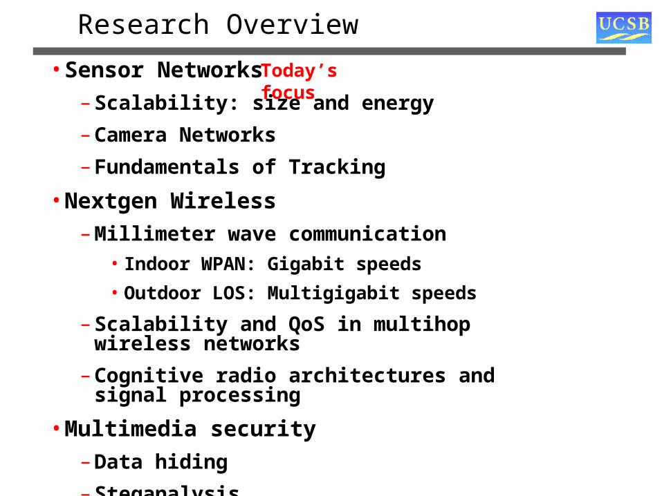
Research Overview

• Sensor Networks– Scalability: size and energy

– Camera Networks

– Fundamentals of Tracking

• Nextgen Wireless– Millimeter wave communication

• Indoor WPAN: Gigabit speeds

• Outdoor LOS: Multigigabit speeds

– Scalability and QoS in multihop wireless networks

– Cognitive radio architectures and signal processing

• Multimedia security– Data hiding

– Steganalysis

Today’s focus

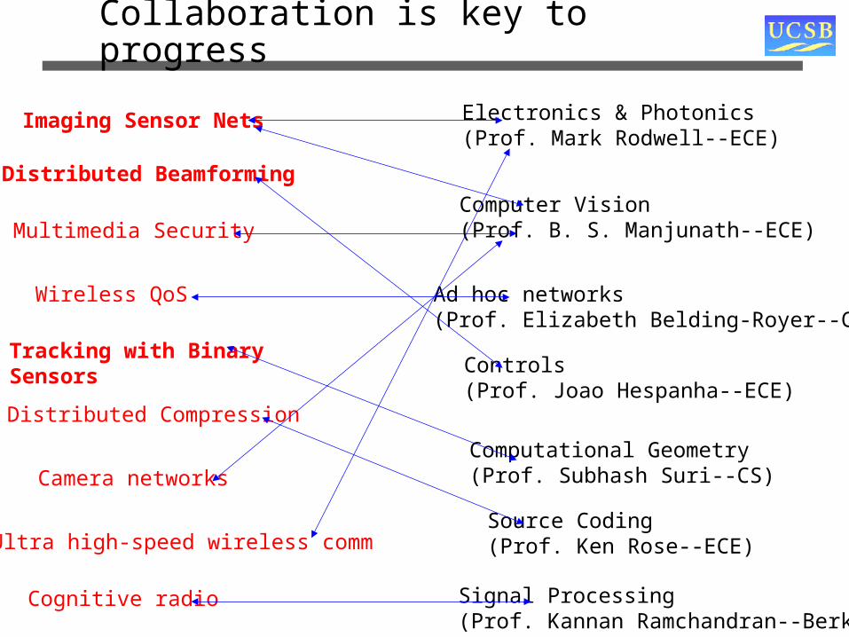
Collaboration is key to progress

Ad hoc networks(Prof. Elizabeth Belding-Royer--CS)

Electronics & Photonics(Prof. Mark Rodwell--ECE)

Computer Vision(Prof. B. S. Manjunath--ECE)

Controls(Prof. Joao Hespanha--ECE)

Computational Geometry(Prof. Subhash Suri--CS)

Imaging Sensor Nets

Distributed Beamforming

Multimedia Security

Wireless QoS

Tracking with BinarySensors

Distributed Compression

Camera networks

Ultra high-speed wireless commSource Coding(Prof. Ken Rose--ECE)

Cognitive radio Signal Processing(Prof. Kannan Ramchandran--Berkeley)

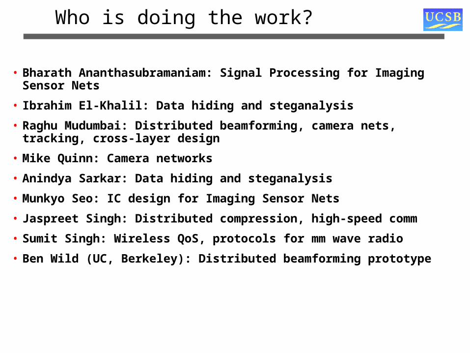
Who is doing the work?

• Bharath Ananthasubramaniam: Signal Processing for Imaging Sensor Nets

• Ibrahim El-Khalil: Data hiding and steganalysis

• Raghu Mudumbai: Distributed beamforming, camera nets, tracking, cross-layer design

• Mike Quinn: Camera networks

• Anindya Sarkar: Data hiding and steganalysis

• Munkyo Seo: IC design for Imaging Sensor Nets

• Jaspreet Singh: Distributed compression, high-speed comm

• Sumit Singh: Wireless QoS, protocols for mm wave radio

• Ben Wild (UC, Berkeley): Distributed beamforming prototype

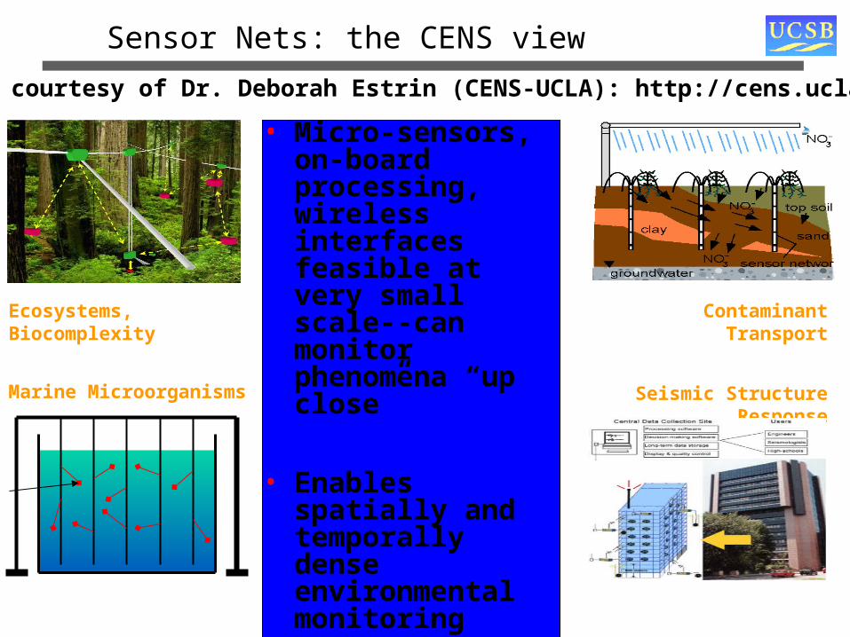
Sensor Nets: the CENS view

• Micro-sensors, on-board processing, wireless interfaces feasible at very small scale--can monitor phenomena “up close”

• Enables spatially and temporally dense environmental monitoring

Embedded Networked Sensing will reveal previously unobservable phenomena

Contaminant TransportEcosystems, Biocomplexity

Marine Microorganisms Seismic Structure Response

Slide courtesy of Dr. Deborah Estrin (CENS-UCLA): http://cens.ucla.edu

Sensor Nets Today

• Berkeley motes continue to prove their worth

– Impact on science

– Promising for DoD and security applications

• Scalability of flat architectures limited to 100s of nodes

– Enough for many applications

– Hierarchical architectures can help

• But we are far from the sci-fi vision of Smart Dust

– Hundreds of thousands of randomly deployed sensors

– Dumb sensors that get smarter by working together

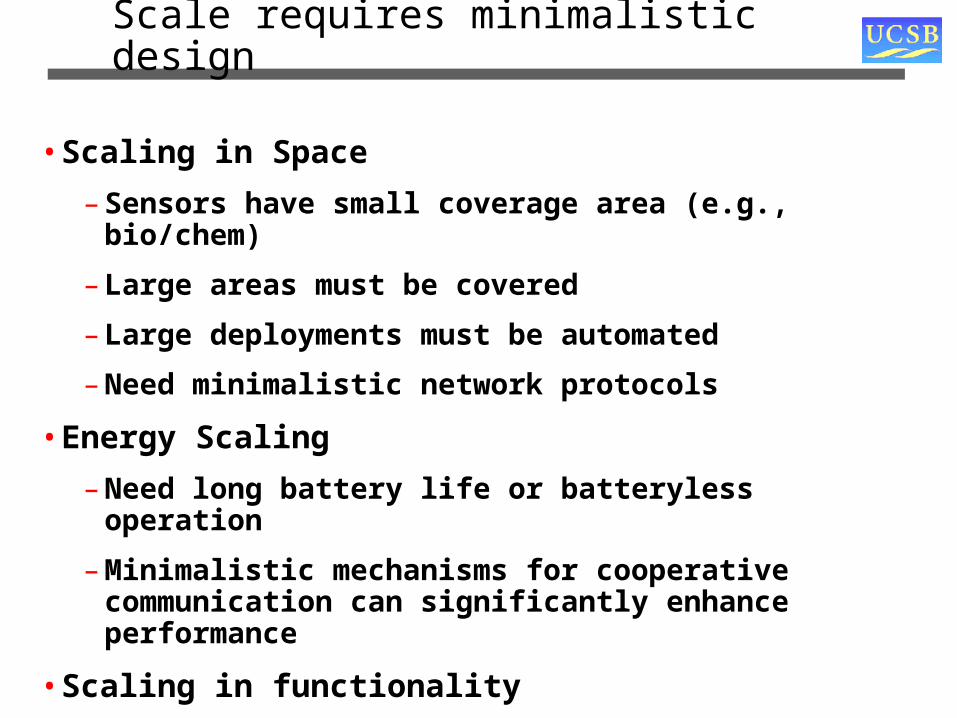
Scale requires minimalistic design

• Scaling in Space

– Sensors have small coverage area (e.g., bio/chem)

– Large areas must be covered

– Large deployments must be automated

– Need minimalistic network protocols

• Energy Scaling

– Need long battery life or batteryless operation

– Minimalistic mechanisms for cooperative communication can significantly enhance performance

• Scaling in functionality

– Small, inexpensive, noisy, failure-prone microsensors

– Need minimalistic sensing models

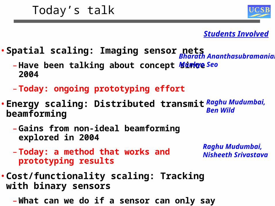
Today’s talk

• Spatial scaling: Imaging sensor nets

– Have been talking about concept since 2004

– Today: ongoing prototyping effort

• Energy scaling: Distributed transmit beamforming

– Gains from non-ideal beamforming explored in 2004

– Today: a method that works and prototyping results

• Cost/functionality scaling: Tracking with binary sensors

– What can we do if a sensor can only say yes or no?

– Today: Fundamental limits, minimal descriptions, algorithms

Students Involved

Bharath Ananthasubramaniam,Munkyo Seo

Raghu Mudumbai,Ben Wild

Raghu Mudumbai,Nisheeth Srivastava

Imaging Sensor Nets

Imaging Sensor Nets: the Concept

Field of simple, low-power sensors dispersed across field of view Cast on ground from truck, plane, or satellite

Sensor as pixels (“dumb dust”) Electronically reflect, with data modulation, beacon from collector (“virtual radar”) Minimal functionality: no GPS, no inter-sensor networking Lifetime of year on watch cell battery

Sophisticated collector Radar and image processing, multiuser data demodulation Joint localization and data collection

Range varies from 100m to 100 km Active versus “passive” sensors, collector characteristics

vast numbers of low-complexity "dumb" pixelssensor + RF transducer + antenna.

collector: satellite

base station on UAV

Sensor fieldSensor field

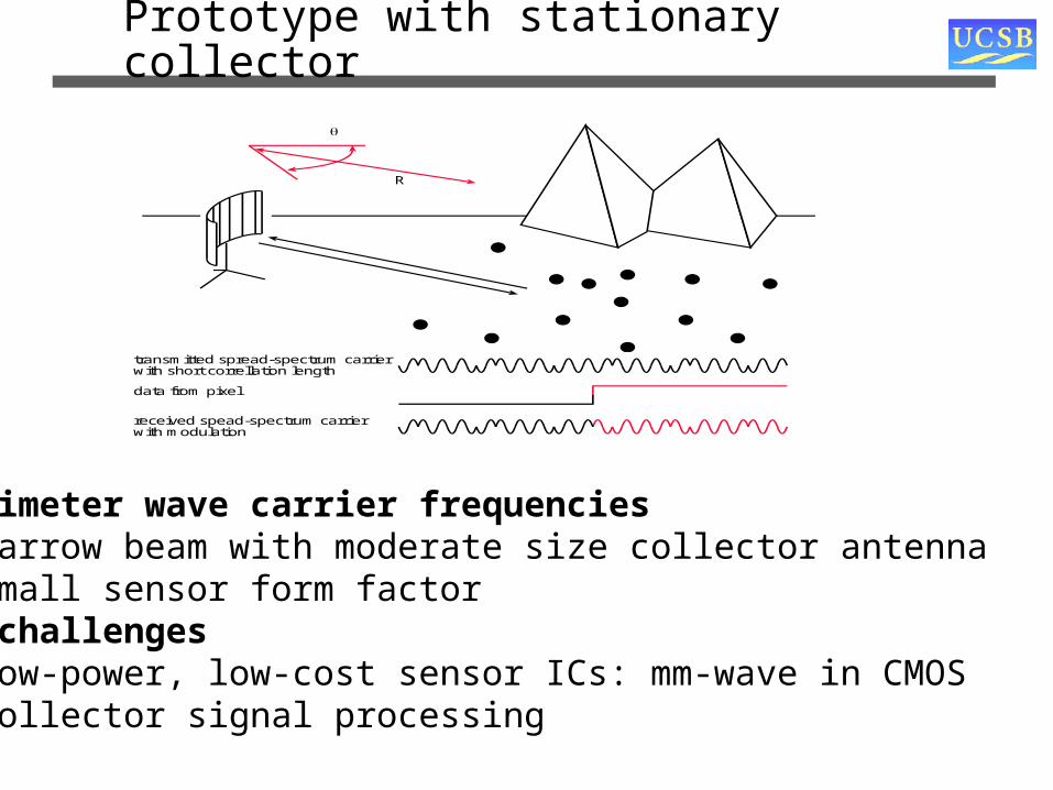
Prototype with stationary collector

R

θ

transmitted spread-spectrum carrierwith short correllation length

data from pixel

received spead-spectrum carrierwith modulation

Millimeter wave carrier frequencies Narrow beam with moderate size collector antenna Small sensor form factorKey challenges Low-power, low-cost sensor ICs: mm-wave in CMOS Collector signal processing

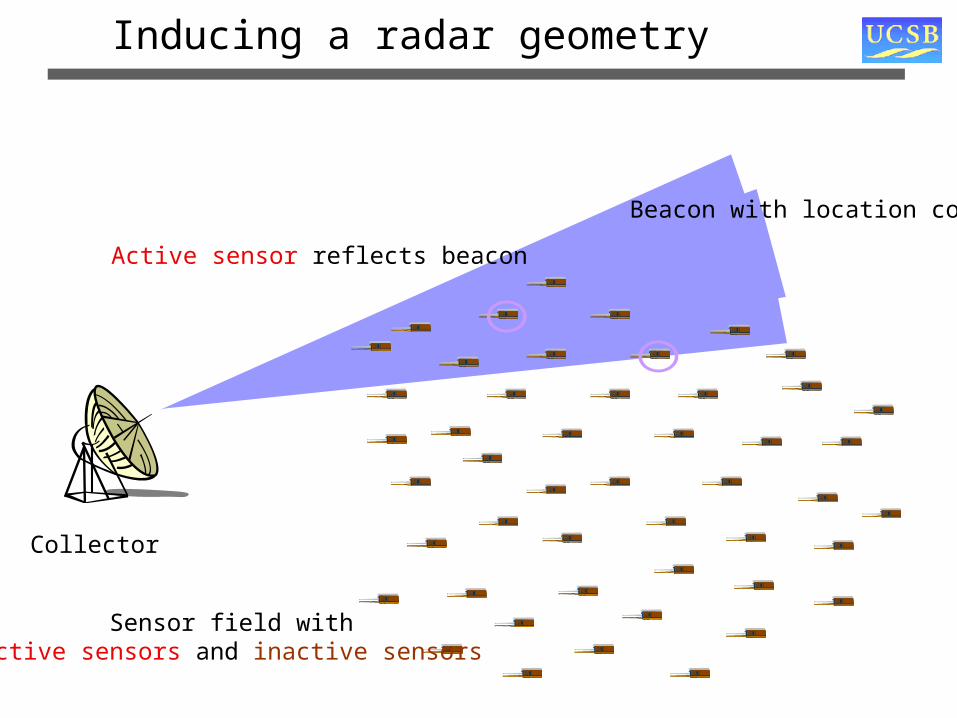
Collector

Beacon with location code

Sensor field withactive sensors and inactive sensors

Active sensor reflects beacon

Inducing a radar geometry

Basic Link Diagram

PRBS

DATA

Jointly detect DATA and DELAY

Collector

Sensor

BPSK modulation

updowndelta fff −=

upf

downf

downf

PRBSf

TXcollD ,

RXcollD ,

RXsensD ,

TXsensD ,

DOWN-LINK

UP-LINK

Freq. shift to filter out ground return

Hierarchy of Challenges

Circuit-level

Technology-level

Link-level

Detection/Estimation

Imaging Algorithm

Application interface

Mm-wave Design

IC technology Substrate/Package/Integration

Signal/ImageProcessing

Low-power, mm-wave circuit designEfficient, low-loss antennaInterconnect

Sensor architectureLink budget calculationCollector phased array design

Estimation for asynchronous modulationLimited precision samples

Nonideal beam patternsIntegrating soft info

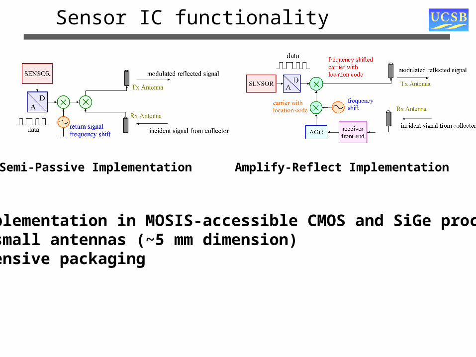
Sensor IC functionality

Semi-Passive Implementation Amplify-Reflect Implementation

IC implementation in MOSIS-accessible CMOS and SiGe processesVery small antennas (~5 mm dimension)Inexpensive packaging

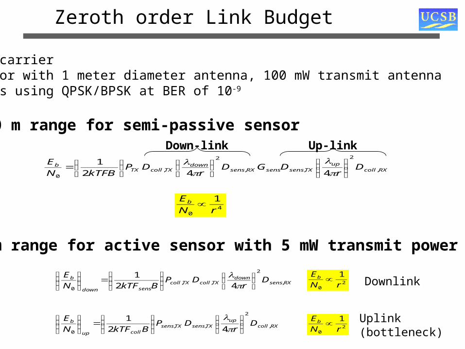
Zeroth order Link Budget

RXcollup

TXsenssensRXsensdown

TXcollTXb D

rDGD

rDP

kTFBN

E,

2

,,

2

,0 442

1⎟⎟⎠

⎞⎜⎜⎝

⎛⎟⎠

⎞⎜⎝

⎛⎟⎠

⎞⎜⎝

⎛=πλ

πλ

Down-link Up-link

40

1

rN

Eb ∝

75 GHz carrierCollector with 1 meter diameter antenna, 100 mW transmit antenna100 Kbps using QPSK/BPSK at BER of 10-9

300 m range for semi-passive sensor

100 km range for active sensor with 5 mW transmit power

RXsensdown

TXcollTXcollsensdown

b Dr

DPBkTFN

E,

2

,,0 42

1⎟⎠

⎞⎜⎝

⎛⎟⎟⎠

⎞⎜⎜⎝

⎛=⎟⎟

⎠

⎞⎜⎜⎝

⎛

πλ

RXcollup

TXsensTXsenscollup

b Dr

DPBkTFN

E,

2

,,0 42

1⎟⎟⎠

⎞⎜⎜⎝

⎛⎟⎟⎠

⎞⎜⎜⎝

⎛=⎟⎟

⎠

⎞⎜⎜⎝

⎛

πλ

20

1

rN

Eb ∝

20

1

rN

Eb ∝

Downlink

Uplink(bottleneck)

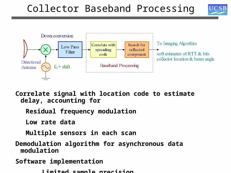
Collector Baseband Processing

Correlate signal with location code to estimate delay, accounting for

Residual frequency modulation

Low rate data

Multiple sensors in each scan

Demodulation algorithm for asynchronous data modulation

Software implementation

Limited sample precision

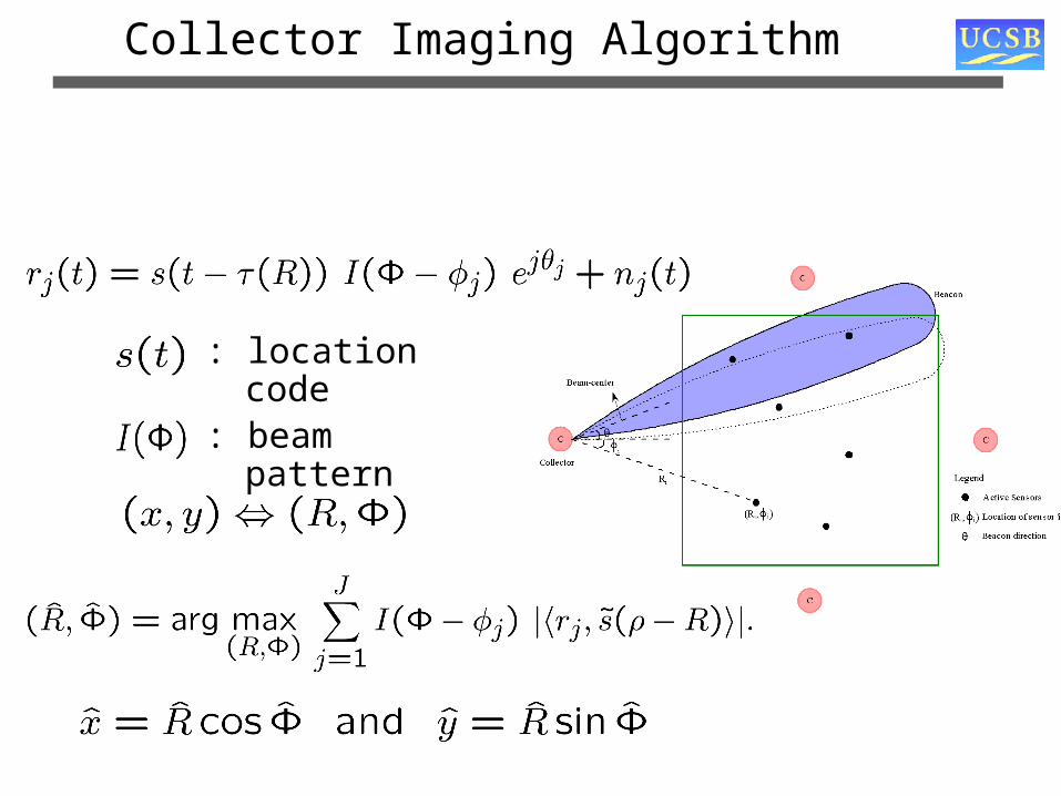
Collector Imaging Algorithm

: location code

: beam pattern

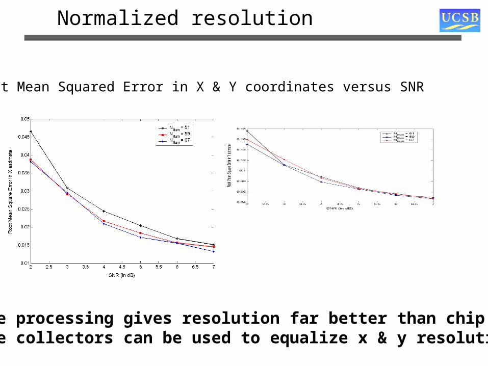
Normalized resolution

Root Mean Squared Error in X & Y coordinates versus SNR

SAR-like processing gives resolution far better than chip durationMultiple collectors can be used to equalize x & y resolution

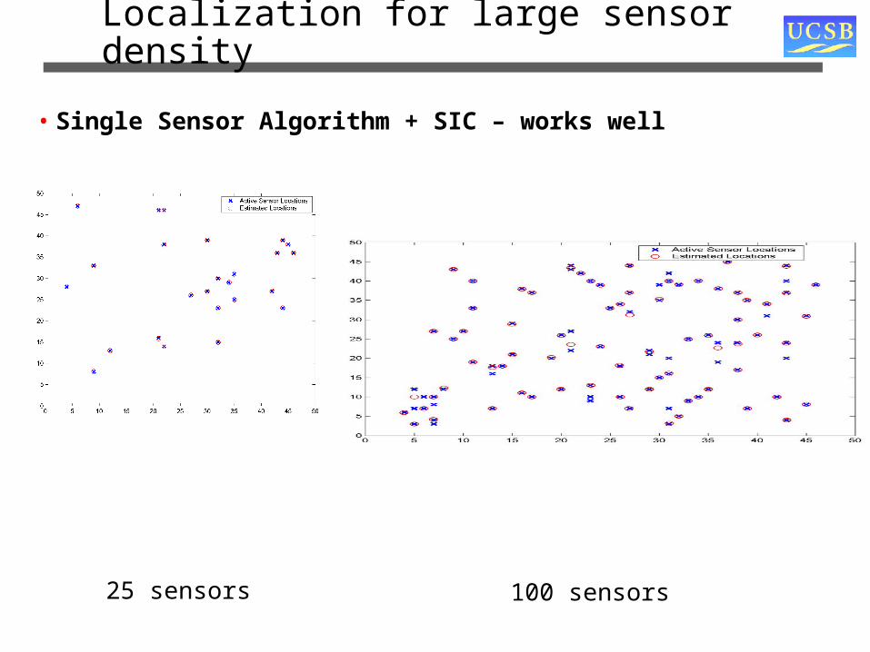
Localization for large sensor density

• Single Sensor Algorithm + SIC – works well

25 sensors 100 sensors

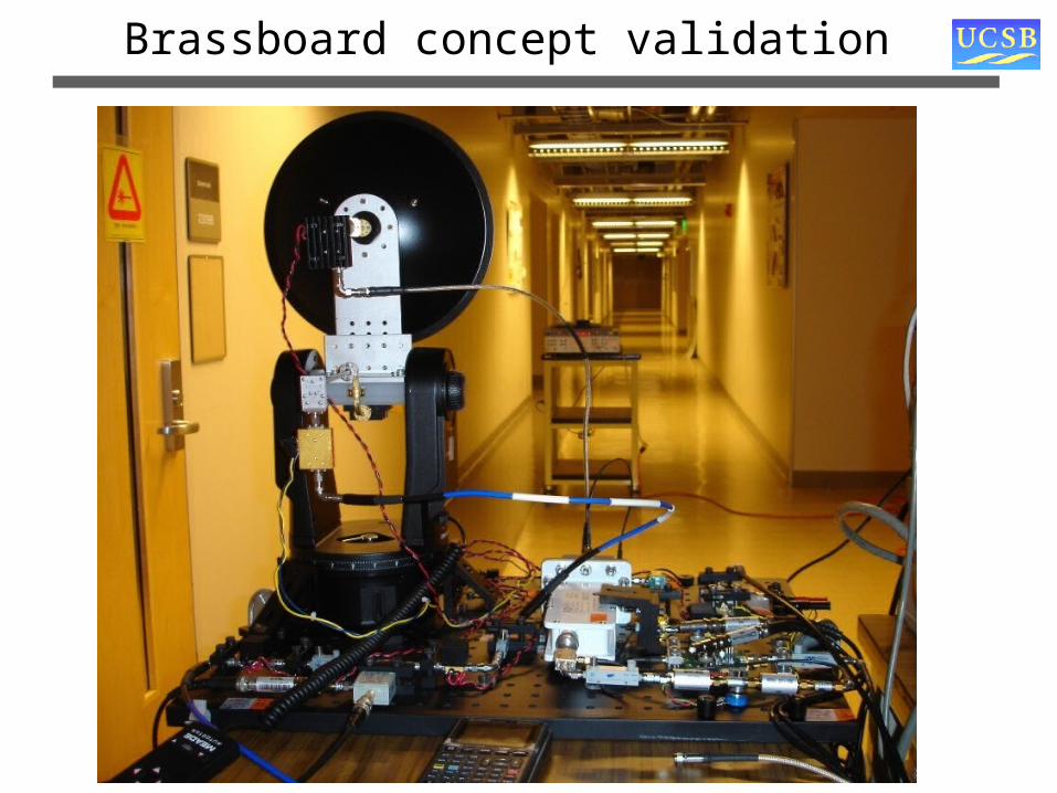
Brassboard concept validation

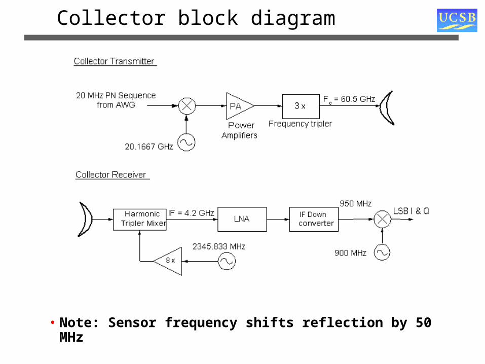
Collector block diagram

• Note: Sensor frequency shifts reflection by 50 MHz

Brassboarded collector and sensor

Collector Sensor

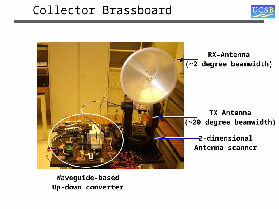
Collector Brassboard

RX-Antenna(~2 degree beamwidth)

TX Antenna(~20 degree beamwidth)

Waveguide-basedUp-down converter

2-dimensionalAntenna scanner

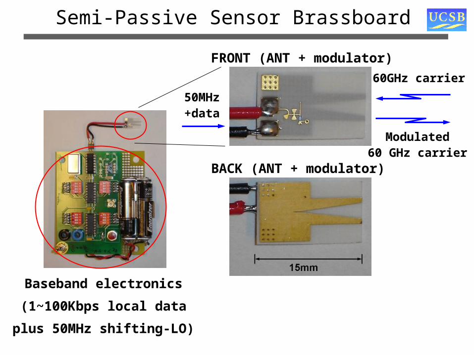
Semi-Passive Sensor Brassboard

Baseband electronics

(1~100Kbps local data

plus 50MHz shifting-LO)

FRONT (ANT + modulator)

BACK (ANT + modulator)

60GHz carrier

Modulated60 GHz carrier

50MHz+data

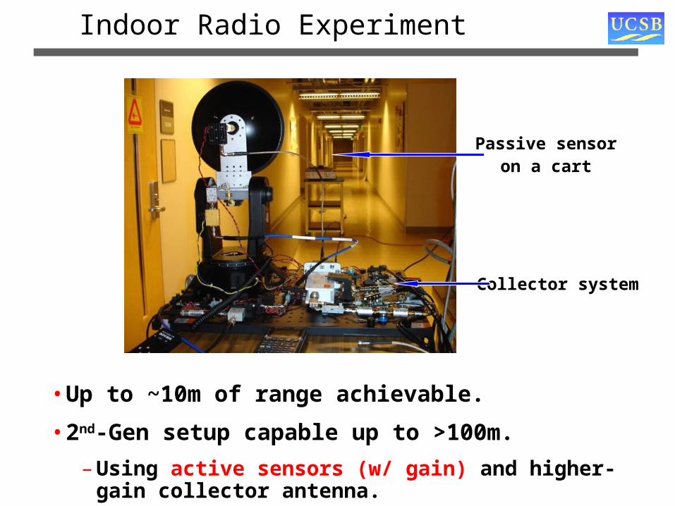
Indoor Radio Experiment

• Up to ~10m of range achievable.

• 2nd-Gen setup capable up to >100m.

– Using active sensors (w/ gain) and higher-gain collector antenna.

Passive sensoron a cart

Collector system

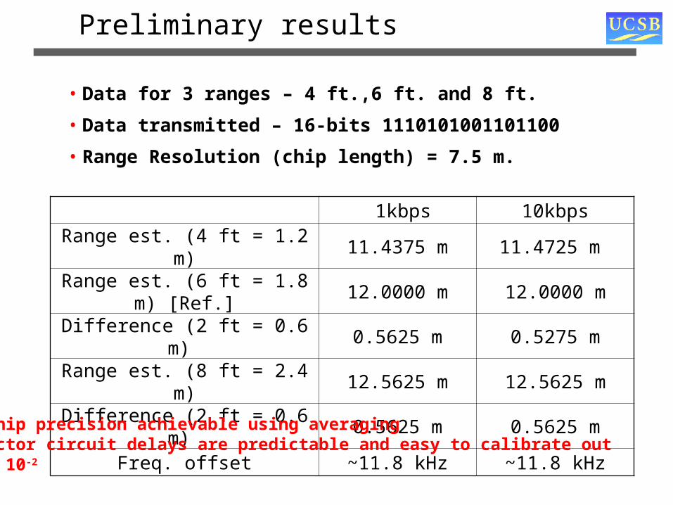
Preliminary results

• Data for 3 ranges – 4 ft.,6 ft. and 8 ft.

• Data transmitted – 16-bits 1110101001101100

• Range Resolution (chip length) = 7.5 m.

1kbps 10kbpsRange est. (4 ft = 1.2 m) 11.4375 m 11.4725 m

Range est. (6 ft = 1.8 m) [Ref.] 12.0000 m 12.0000 mDifference (2 ft = 0.6 m) 0.5625 m 0.5275 mRange est. (8 ft = 2.4 m) 12.5625 m 12.5625 mDifference (2 ft = 0.6 m) 0.5625 m 0.5625 m

Freq. offset ~11.8 kHz ~11.8 kHz

Sub-chip precision achievable using averaging Collector circuit delays are predictable and easy to calibrate outBER ~ 10-2

Future Work

• Collector Hardware/Processing

– Azimuth data collection – from computer by controlling antenna pointing direction

– Azimuth processing to improve effective SNR/ Range

– Upgrade PA to 200mW (full power) to perform outdoor ranging experiments. (with FCC permission)

– Integrate collector components into IC

• Sensor ICs

• Complete Design of “Passive” Sensor CMOS IC

• Work towards the Active ICs

Imaging Sensor Nets: Current Status

• Lab-scale mm wave experiment to verify link budgets

– Basic concept has been verified

– Baseband software (version 1) has been developed

• Brassboard to-dos

– Azimuth data collection

– Higher power transmission to increase range (awaiting FCC OK)

• IC design for semi-passive sensor

• IC design for active sensor

– Need creative solution for isolation problems

• Many open system level issues

– Data representation/compression, redundancy

– Exploiting multiple collectors

– Sensor-driven imaging sensor nets

Distributed Beamforming

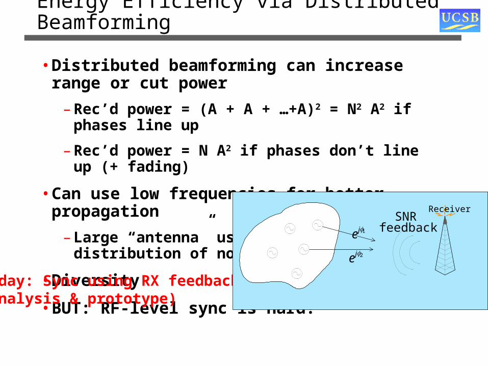
Energy Efficiency via Distributed Beamforming

• Distributed beamforming can increase range or cut power

– Rec’d power = (A + A + …+A)2 = N2 A2 if phases line up

– Rec’d power = N A2 if phases don’t line up (+ fading)

• Can use low frequencies for better propagation

– Large “antenna” using natural spatial distribution of nodes

• Diversity

• BUT: RF-level sync is hard!

Today: Sync using RX feedback(analysis & prototype)

Receiver

1je

2je

SNRfeedback

Feedback Control Mechanism

• Initially the carrier phases are unknown • Each timeslot, the transmitters try a random phase correction

•Keep the corrections that increase SNR, discard the others• Carrier phases become more and more aligned• Phase coherence achieved in time linear in number of nodes

Typical phase evolution(10 nodes)

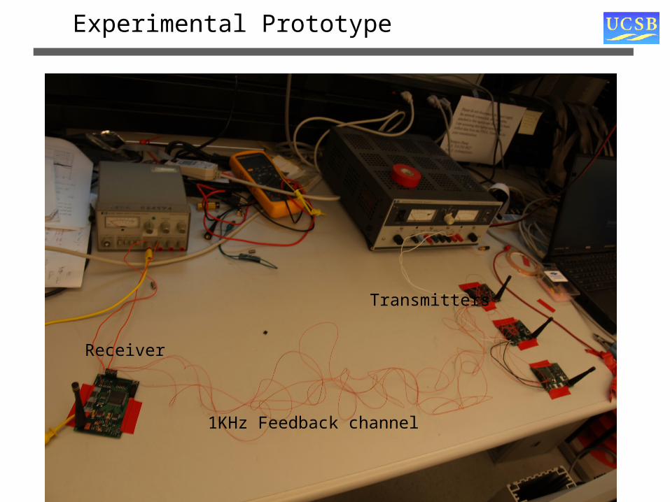
Experimental Prototype

Receiver

Transmitters

1KHz Feedback channel

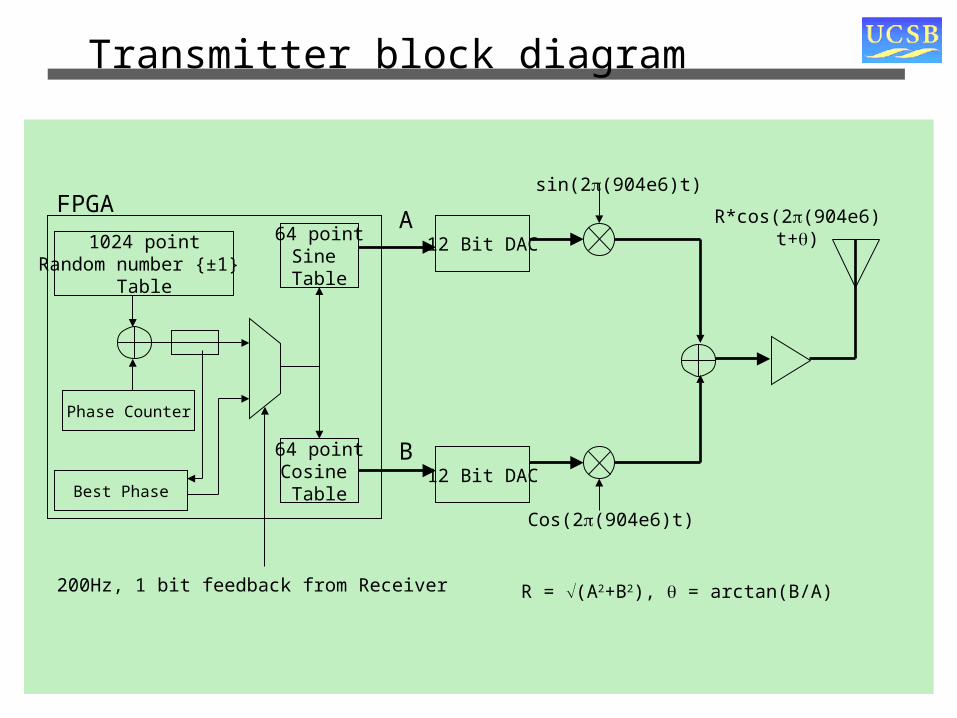
Transmitter block diagram

12 Bit DAC

FPGA

200Hz, 1 bit feedback from Receiver

12 Bit DAC

Cos(2π(904e6)t)

R*cos(2π(904e6)t+θ)64 point

Sine Table

64 pointCosine Table

1024 pointRandom number {±1}

Table

Phase Counter

Best Phase

A

B

sin(2π(904e6)t)

R = (A2+B2), θ = arctan(B/A)

Receiver block diagram

904 MHz Bandpass Filter,

20MHz BW cos(2π(904e6+fIF)t)

904 MHz Signal

sin(2π(904e6+fIF)t)

1MSPS,16 Bit ADC

1MSPS,16 Bit ADC

20kHz IF to avoid problems with Direct Conversion to DC

12 Bit DAC

Oscilloscope

FPGA

( · )2

( · )2

5000Sample average

200Hz 1 bit feedback to beamformers

Power (i)

Power (i) >? Power(i-1,..,i-M-1) {M=4 for results shown}

time

Pow

er

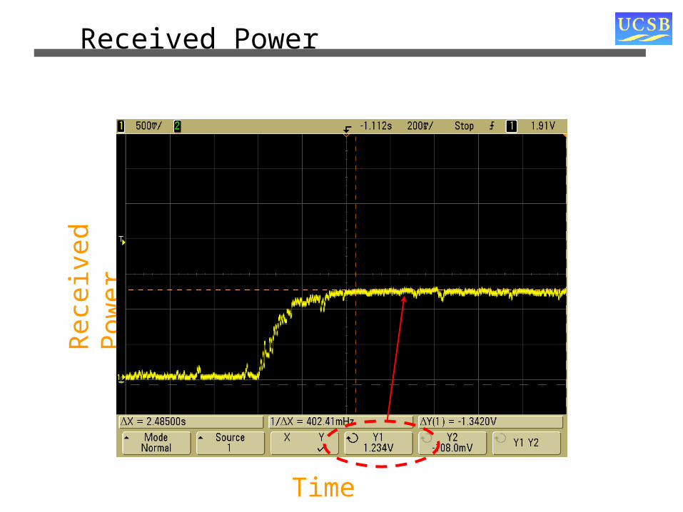
Received PowerR

ecei

ved

Pow

er

Time

Need to get data for this.

Conclusions from prototype

• Distributed beamforming works!

• Key technical challenges– Phase jitter: Highly sensitive to PLL loop-filter

– Power measurement for modulated signals

• Limitations– Small-scale experiment (only 3 transmitters)

– Static channel conditions

Towards an analytical model

• Empirical observation: convergence is highly predictable

y[n+1]

α.y[n] x1

x2

Net effect of phase perturbations

What can we say about the distributions of x1 and x2?(without knowing all the individual transmitter phases)

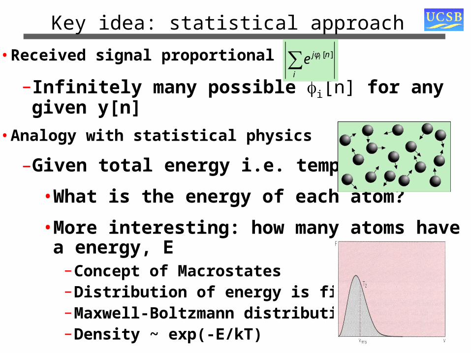
Key idea: statistical approach

•Received signal proportional to

–Infinitely many possible i[n] for any given y[n]

•Analogy with statistical physics

–Given total energy i.e. temperature

•What is the energy of each atom?

•More interesting: how many atoms have a energy, E–Concept of Macrostates–Distribution of energy is fixed–Maxwell-Boltzmann distribution–Density ~ exp(-E/kT)

∑i

nj ie ][φ

The “exp-cosine” distribution

• Initially i[0] is uniform in (-π, π]

• The phases i[n] get more and more clustered

• Given , what is the distribution of i[n]?

– “Typical” distribution closest in KL distance to uniform

– The Conditional Limit Theorem

The “exp-cosine” distribution

€

f (φ) = exp(λ cosφ) /I0(λ )

€

E[cosφ] =I1(λ )

I0(λ )= y[n]/N

€

| cosφii∑ |≈ NE[cosφ] = y[n]

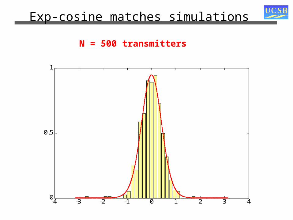
Exp-cosine matches simulations

-4 -3 -2 -1 0 1 2 3 40

0.5

1

Phase Angles in radians

Probability density N = 500 transmitters

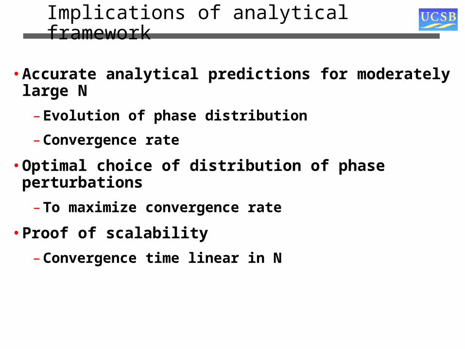
Implications of analytical framework

• Accurate analytical predictions for moderately large N

– Evolution of phase distribution

– Convergence rate

• Optimal choice of distribution of phase perturbations

– To maximize convergence rate

• Proof of scalability

– Convergence time linear in N

Accurate prediction of trajectory

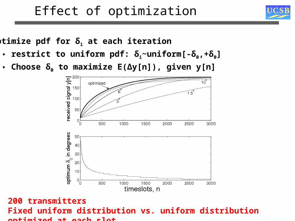
Effect of optimization

200 transmittersFixed uniform distribution vs. uniform distribution optimized at each slot

•Optimize pdf for δi at each iteration

• restrict to uniform pdf: δi~uniform[-δ0,+δ0]

• Choose δ0 to maximize E(Δy[n]), given y[n]

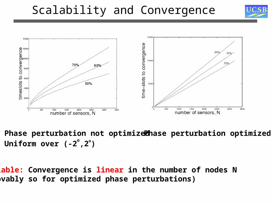
Scalability and Convergence

Phase perturbation not optimizedUniform over (-2

o,2o)

Phase perturbation optimized

Scalable: Convergence is linear in the number of nodes N(provably so for optimized phase perturbations)

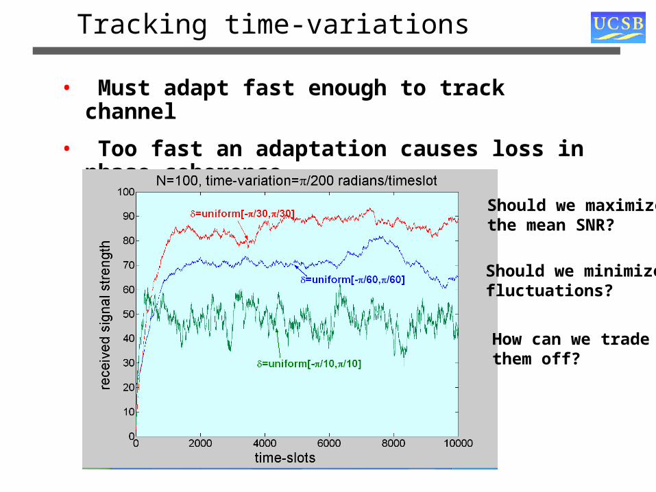
Tracking time-variations

• Must adapt fast enough to track channel

• Too fast an adaptation causes loss in phase coherence

Should we maximizethe mean SNR?

Should we minimizefluctuations?

How can we tradethem off?

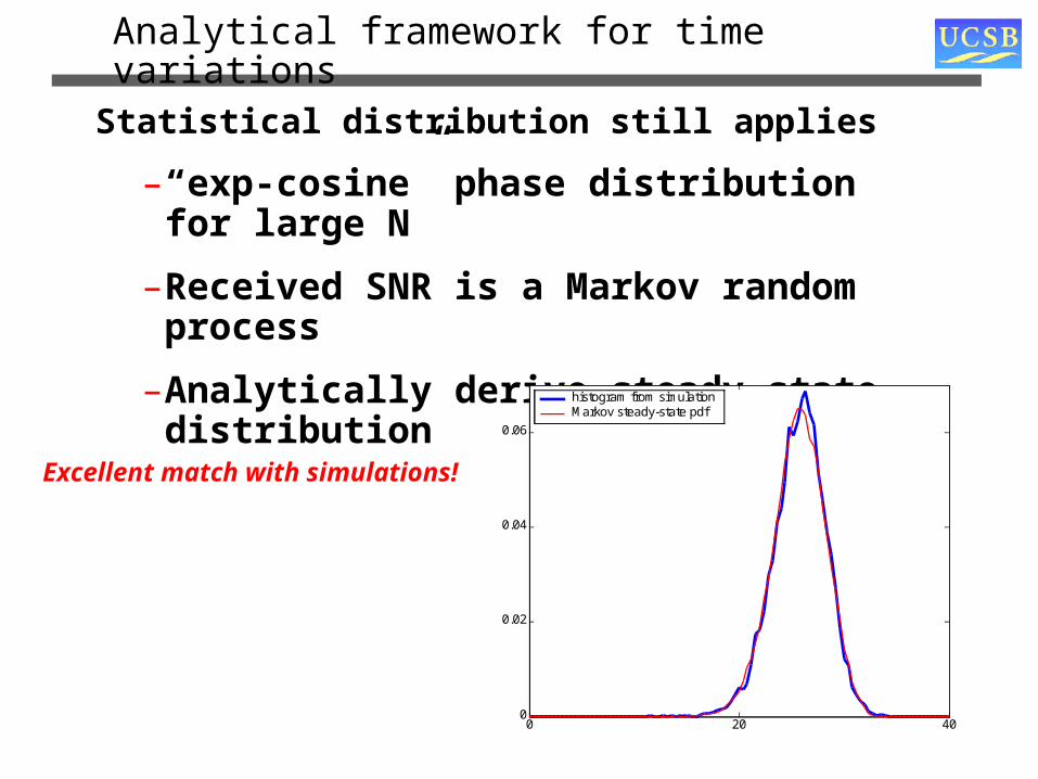
Analytical framework for time variations

Statistical distribution still applies

– “exp-cosine” phase distribution for large N

– Received SNR is a Markov random process

– Analytically derive steady-state distribution

0 20 400

0.02

0.04

0.06

Prob. density, f

ss(

y)

received signal strength, y

histogram from simulationMarkov steady-state pdf

Excellent match with simulations!

Distributed Beamforming: Current Status

• We now know it works

– 3 node prototype gives 90% of maximum possible gains

• Analytical framework accurately predicts performance

– Need simple rules of thumb for time-varying channels

– Better justification of exp-cosine derivation

• Applications go beyond sensor nets

– Wireless link protocols building on distributed beamforming?

• Generalization to other distributed control tasks?

Tracking with binary proximity sensors

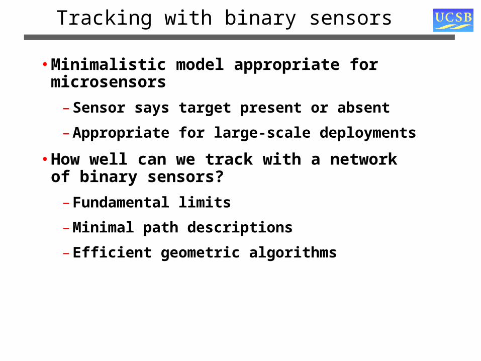
Tracking with binary sensors

• Minimalistic model appropriate for microsensors

– Sensor says target present or absent

– Appropriate for large-scale deployments

• How well can we track with a network of binary sensors?

– Fundamental limits

– Minimal path descriptions

– Efficient geometric algorithms

The Geometry of Binary Sensing

Target Path

Sensor Outputs

Localization patches

Localization arcs

Results

• Attainable resolution ~ 1/(sensor density*sensing range)

• Spatial low pass filtering

– Path variations faster than resolution cannot be tracked

– We can track “lowpass” version of the path

• OccamTrack algorithm

– Constructs minimal piecewise linear path representations

– Provides velocity estimates for “lowpass” version

• Robustness to sensing range variation

– Original OccamTrack can get into trouble

– Particle filtering algorithm + Geometric clean-up

• Lab-scale experiments

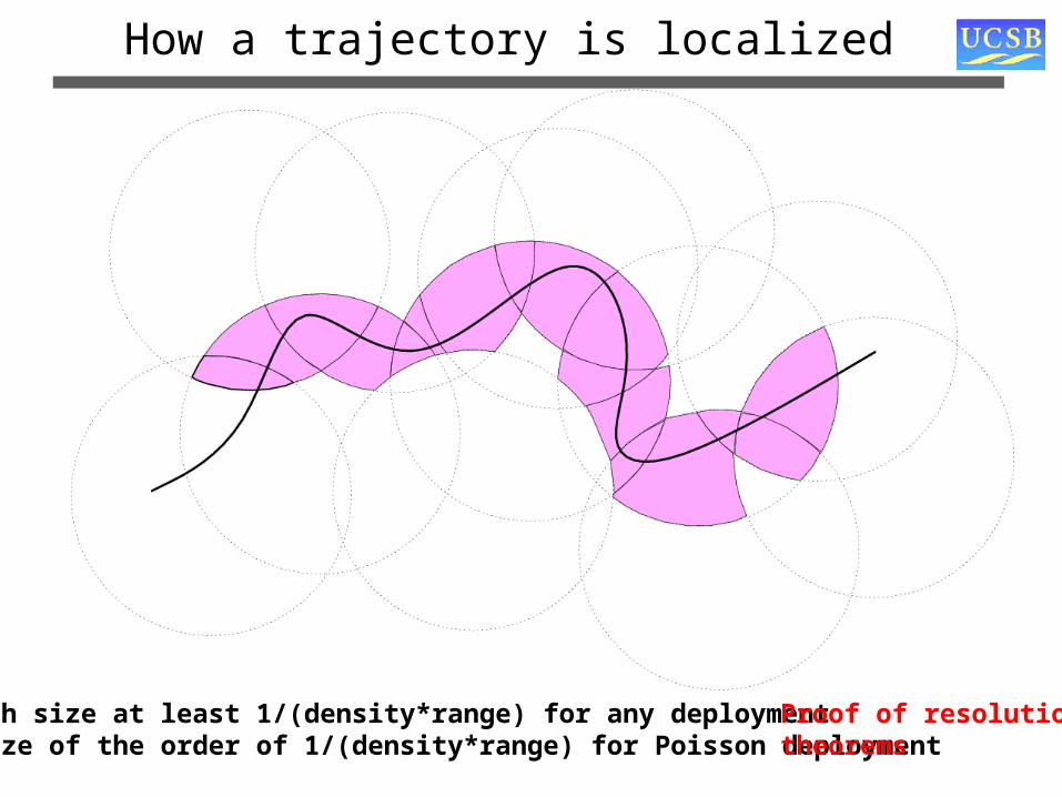
How a trajectory is localized

Max patch size at least 1/(density*range) for any deploymentPatch size of the order of 1/(density*range) for Poisson deployment

Proof of resolutiontheorems

Minimal representation: OccamTrack

Greedy algorithm for piecewise linear representation:Draw lines stabbing localization arcs that are as long as possible

Spatial Lowpass Filtering

Cannot capture rapid variationsCan only reconstruct “lowpass” version of pathJustifies piecewise linear representation

Velocity estimation and minimal representation

Which path should we use to estimate (lowpass version of) velocity? We can be off by a factor of two! A simple formula: dv/v = dL/LProposition: If piecewise linear approx works well, then velocity estimate is accurate.

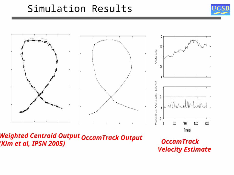
OccamTrackVelocity Estimate

OccamTrack OutputWeighted Centroid Output(Kim et al, IPSN 2005)

Simulation Results

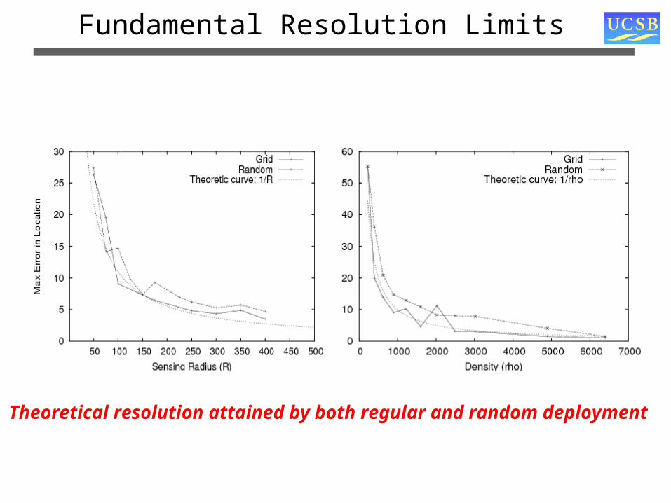
Fundamental Resolution Limits

Theoretical resolution attained by both regular and random deployment

Handling non-ideal sensing

Detected

Not detected

?

A simple model

Localization patch = intersection of outer circles with complements of inner circlesParticle filtering algorithm provides robust performanceGeometric clean-up provides minimal description

Acoustic sensors are unreliable & unpredictable

Low pass filterobservations

Experiment with acoustic sensor

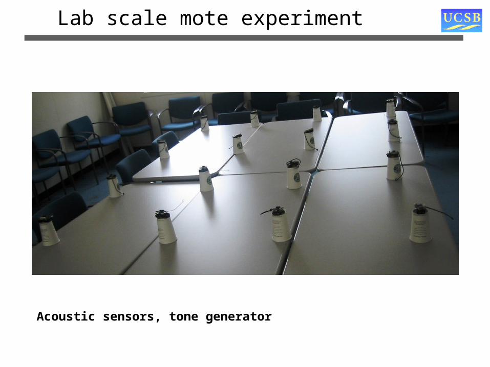
Lab scale mote experiment

Acoustic sensors, tone generator

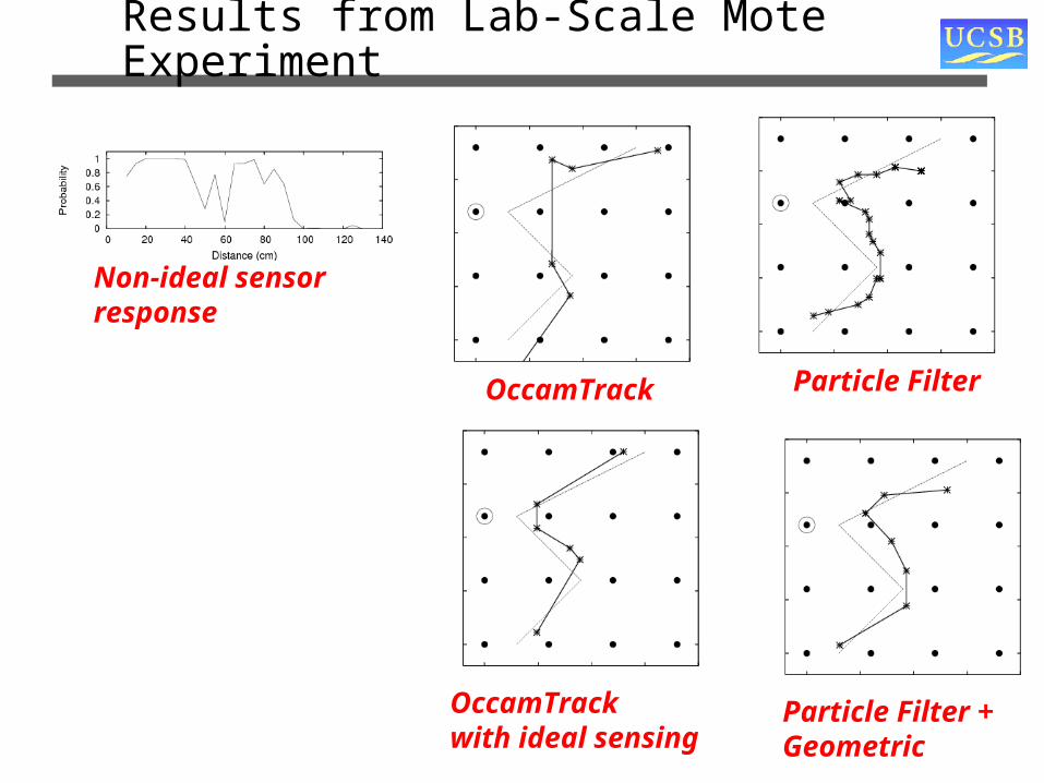
OccamTrack Particle Filter

Particle Filter +Geometric

OccamTrack with ideal sensing

Results from Lab-Scale Mote Experiment

Non-ideal sensorresponse

Tracking with Binary Sensors: Current Status

• Low-cost microsensors can be very useful for tracking

– Small range can be compensated for by dense deployment

– Random deployment works

– Fundamental limits identified and attained

– Algorithms can be made robust to non-ideal sensing

• Current work focuses on multiple targets

– Can we count them reliably?

– How well can we track?

Challenges ahead: a sampling

• Sensor Networks

– Imaging Sensor Nets: making them happen

– Architectures for in-network processing and collaboration

– Comprehensive solutions for flagship applications

– The role of distributed control

– Visual sensor networks

• Ultra high-speed communication

– Cross-layer design of mm wave networks

– The ADC bottleneck

• Multihop multimedia comm

– Video through the home

– Voice in emergency plug-and-play networks