minimizing a submodular function from samples
TRANSCRIPT

Minimizing a Submodular Function from Samples
Eric BalkanskiHarvard University
Yaron SingerHarvard University
Abstract
In this paper we consider the problem of minimizing a submodular function fromtraining data. Submodular functions can be efficiently minimized and are conse-quently heavily applied in machine learning. There are many cases, however, inwhich we do not know the function we aim to optimize, but rather have accessto training data that is used to learn it. In this paper we consider the question ofwhether submodular functions can be minimized when given access to its trainingdata. We show that even learnable submodular functions cannot be minimizedwithin any non-trivial approximation when given access to polynomially-many sam-ples. Specifically, we show that there is a class of submodular functions with rangein [0, 1] such that, despite being PAC-learnable and minimizable in polynomial-time,no algorithm can obtain an approximation strictly better than 1/2 − o(1) usingpolynomially-many samples drawn from any distribution. Furthermore, we showthat this bound is tight via a trivial algorithm that obtains an approximation of 1/2.
1 Introduction
For well over a decade now, submodular minimization has been heavily studied in machine learning(e.g. [SK10, JB11, JLB11, NB12, EN15, DTK16]). This focus can be largely attributed to the factthat if a set function f : 2N → R is submodular, meaning it has the following property of diminishingreturns: f(S ∪ a) − f(S) ≥ f(T ∪ a) − f(T ) for all S ⊆ T ⊆ N and a 6∈ T , then it canbe optimized efficiently: its minimizer can be found in time that is polynomial in the size of theground set N [GLS81, IFF01]. In many cases, however, we do not know the submodular function,and instead learn it from data (e.g. [BH11, IJB13, FKV13, FK14, Bal15, BVW16]). The questionwe address in this paper is whether submodular functions can be (approximately) minimized whenthe function is not known but can be learned from training data.
An intuitive approach for optimization from training data is to learn a surrogate function from trainingdata that predicts the behavior of the submodular function well, and then find the minimizer of thesurrogate learned and use that as a proxy for the true minimizer we seek. The problem however, is thatthis approach does not generally guarantee that the resulting solution is close to the true minimum ofthe function. One pitfall is that the surrogate may be non-submodular, and despite approximating thetrue submodular function arbitrarily well, the surrogate can be intractable to minimize. Alternatively,it may be that the surrogate is submodular, but its minimum is arbitrarily far from the minimum ofthe true function we aim to optimize (see examples in Appendix A).
Since optimizing a surrogate function learned from data may generally result in poor approximations,one may seek learning algorithms that are guaranteed to produce surrogates whose optima well-approximate the true optima and are tractable to compute. More generally, however, it is possible thatthere is some other approach for optimizing the function from the training samples, without learninga model. Therefore, at a high level, the question is whether a reasonable number of training samplessuffices to minimize a submodular function. We can formalize this as optimization from samples.
31st Conference on Neural Information Processing Systems (NIPS 2017), Long Beach, CA, USA.

Optimization from samples. We will say that a class of functions F = f : 2N → [0, 1] isα-optimizable from samples over distribution D if for every f ∈ F and δ ∈ (0, 1), when givenpoly(|N |) i.i.d. samples (Si, f(Si))mi=1 where Si ∼ D, with probability at least 1 − δ over thesamples one can construct an algorithm that returns a solution S ⊆ N s.t,
f(S)− minT⊆N
f(T ) ≤ α.
This framework was recently introduced in [BRS17] for the problem of submodular maximizationwhere the standard notion of approximation is multiplicative. For submodular minimization, sincethe optimum may have zero value, the suitable measure is that of additive approximations for [0, 1]-bounded functions, and the goal is to obtain a solution which is a o(1) additive approximation to theminimum (see e.g. [CLSW16, EN15, SK10]). The question is then:
Can submodular functions be minimized from samples?
Since submodular functions can be minimized in polynomial-time, it is tempting to conjecture thatwhen the function is learnable it also has desirable approximation guarantees from samples, especiallyin light of positive results in related settings of submodular maximization:
• Constrained maximization. For functions that can be maximized in polynomial time undera cardinality constraint, like modular and unit-demand functions, there are polynomialtime algorithms that obtain an arbitrarily good approximation using polynomially-manysamples [BRS16, BRS17]. For general monotone submodular functions which are NP-hard to maximize under cardinality constraints, there is no algorithm that can obtain areasonable approximation from polynomially-many samples [BRS17]. For the problem ofunconstrained minimization, submodular functions can be optimized in polynomial time;
• Unconstrained maximization. For unconstrained maximization of general submodularfunctions, the problem is NP-hard to maximize (e.g. MAX-CUT) and one seeks constantfactor approximations. For this problem, there is an extremely simple algorithm that usesno queries and obtains a good approximation: choose elements uniformly at random withprobability 1/2 each. This algorithm achieves a constant factor approximation of 1/4 forgeneral submodular functions. For symmetric submodular functions (i.e. f(S) = f(N \S)),this algorithm is a 1/2-approximation which is optimal, since no algorithm can obtain anapproximation ratio strictly better than 1/2 using polynomially-many value queries, evenfor symmetric submodular functions [FMV11]. For unconstrained symmetric submodularminimization, there is an appealing analogue: the empty set and the ground set N areguaranteed to be minimizers of the function (see Section 2). This algorithm, of course, usesno queries either. The parallel between these two problems seems quite intuitive, and itis tempting to conjecture that like for unconstrained submodular maximization, there areoptimization from samples algorithms for general unconstrained submodular minimizationwith good approximation guarantees.
Main result. Somewhat counter-intuitively, we show that despite being computationally tractableto optimize, submodular functions cannot be minimized from samples to within a desirable guarantee,even when these functions are learnable. In particular, we show that there is no algorithm forminimizing a submodular function from polynomially-many samples drawn from any distributionthat obtains an additive approximation of 1/2 − o(1), even when the function is PAC-learnable.Furthermore, we show that this bound is tight: the algorithm which returns the empty set or groundset each with probability 1/2 achieves at least a 1/2 approximation. Notice that this also implies thatin general, there is no learning algorithm that can produce a surrogate whose minima is close to theminima of the function we aim to optimize, as otherwise this would contradict our main result.
Technical overview. At a high level, hardness results in optimization from samples are shownby constructing a family of functions, where the values of functions in the family are likely to beindistinguishable for the samples, while having very different optimizers. The main technical difficultyis to construct a family of functions that concurrently satisfy these two properties (indistinguishabilityand different optimizers), and that are also PAC-learnable. En route to our main construction, wefirst construct a family of functions that are completely indistinguishable given samples drawn fromthe uniform distribution, in which case we obtain a 1/2− o(1) impossibility result (Section 2). The
2

general result that holds for any distribution requires heavier machinery to argue about more generalfamilies of functions where some subset of functions can be distinguished from others given samples.Instead of satisfying the two desired properties for all functions in a fixed family, we show that theseproperties hold for all functions in a randomized subfamily (Section 3.2). We then develop an efficientlearning algorithm for the family of functions constructed for the main hardness result (Section 3.3).This algorithm builds multiple linear regression predictors and a classifier to direct a fresh set to theappropriate linear predictor. The learning of the classifier and the linear predictors relies on multipleobservations about the specific structure of this class of functions.
1.1 Related work
The problem of optimization from samples was introduced in the context of constrained submodularmaximization [BRS17, BRS16]. In general, for maximizing a submodular function under a cardinalityconstraint, no algorithm can obtain a constant factor approximation guarantee from any samples. Asdiscussed above, for special classes of submodular functions that can be optimized in polynomial timeunder a cardinality constraint, and for unconstrained maximization, there are desirable optimizationfrom samples guarantees. It is thus somewhat surprising that submodular minimization, which is anunconstrained optimization problem that is optimizable in polynomial time in the value query model,is hard to optimize from samples. From a technical perspective the constructions are quite different.In maximization, the functions constructed in [BRS17, BRS16] are monotone so the ground setwould be an optimal solution if the problem was unconstrained. Instead, we need to construct novelnon-monotone functions. In convex optimization, recent work shows a tight 1/2-inapproximabilityfor convex minimization from samples [BS17]. Although there is a conceptual connection betweenthat paper and this one, from a technical perspective these papers are orthogonal. The discreteanalogue of the family of convex functions constructed in that paper is not (even approximately) afamily of submodular functions, and the constructions are significantly different.
2 Warm up: the Uniform Distribution
As a warm up to our main impossibility result, we sketch a tight lower bound for the special case inwhich the samples are drawn from the uniform distribution. At a high level, the idea is to construct afunction which considers some special subset of “good” elements that make its value drops when aset contains all such “good” elements. When samples are drawn from the uniform distribution and“good” elements are sufficiently rare, there is a relatively simple construction that obfuscates whichelements the function considers “good”, which then leads to the inapproximability.
2.1 Hardness for uniform distribution
We construct a family of functions F where fi ∈ F is defined in terms of a set Gi ⊂ N of size√n.
For each such function we call Gi the set of good elements, and Bi = N \Gi its bad elements. Wedenote the number of good and bad elements in a set S by gS and bS , dropping the subscripts (S andi) when clear from context, so g = |Gi ∩ S| and b = |Bi ∩ S|. The function fi is defined as follows:
fi(S) :=
1
2+
1
2n· (g + b) if g <
√n
1
2n· b if g =
√n
It is easy to verify that these functions are submodular with range in [0, 1] (see illustration inFigure 1a). Given samples drawn uniformly at random (u.a.r.), it is impossible to distinguish goodand bad elements since with high probability (w.h.p.) g <
√n for all samples. Informally, this
implies that a good learner for F over the uniform distribution D is f ′(S) = 1/2 + |S|/(2n).Intuitively, F is not 1/2− o(1) optimizable from samples because if an algorithm cannot learn theset of good elements Gi, then it cannot find S such fi(S) < 1/2− o(1) whereas the optimal solutionS?i = Gi has value fi(Gi) = 0.
Theorem 1. Submodular functions f : 2N → [0, 1] are not 1/2 − o(1) optimizable from samplesdrawn from the uniform distribution for the problem of submodular minimization.
3

Proof. The details for the derivation of concentration bounds are in Appendix B. Consider fk drawnu.a.r. from F and let f? = fk and G? = Gk. Since the samples are all drawn from the uniformdistribution, by standard application of the Chernoff bound we have that every set Si in the samplerespects |Si| ≤ 3n/4, w.p. 1 − e−Ω(n). For sets S1, . . . , Sm, all of size at most 3n/4, when fj isdrawn u.a.r. from F we get that |Si ∩ Gj | <
√n, w.p. 1 − e−Ω(n1/2) for all i ∈ [m], again by
Chernoff, and since m = poly(n). Notice that this implies that w.p. 1− e−Ω(n1/2) for all i ∈ [m]:
fj(Si) =1
2+|Si|2n
Now, let F ′ be the collection of all functions fj for which fj(Si) = 1/2 + |Si|/(2n) on all setsSimi=1. The argument above implies that |F ′| = (1− e−Ω(n1/2))|F|. Thus, since f? is drawn u.a.r.from F we have that f? ∈ F ′ w.p. 1− e−Ω(n1/2), and we condition on this event.
Let S be the (possibly randomized) solution returned by the algorithm. Observe that S is independentof f? ∈ F ′. In other words, the algorithm cannot learn any information about which function in F ′
generates the samples. By Chernoff, if we fix S and choose f u.a.r. from F , then, w.p. 1− e−Ω(n1/6):
f(S) ≥ 1
2− o(1)
Thus, since |F ′| = (1 − e−Ω(n1/2))|F|, w.p. 1 − e−Ω(n1/6) over the choice of f?, we have thatf?(S) ≥ 1/2− o(1) and we condition on this event. Conditioning on all events, the value of the setS returned by the algorithm is 1/2− o(1) whereas the optimal solution is f?(G?) = 0. Since all theevents we conditioned on occur with exponentially high probability, this concludes the proof.
2.2 A tight upper bound
We now show that the result above is tight. In particular, by randomizing between the empty set andthe ground set we get a solution whose value is at most 1/2. In the case of symmetric submodularfunctions, the empty set and the ground set are minima. Notice, that this does not require any samples.Proposition 2. The algorithm which returns the empty set ∅ or the ground N with probability 1/2each is a 1/2 additive approximation for the problem of unconstrained submodular minimization.
Proof. Let S ⊆ N , observe that
f(N \ S)− f(∅) = f∅(N \ S) ≥ fS(N \ S) = f(N)− f(S)where the inequality is by submodularity. Thus, we obtain
1
2(f(N) + f(∅)) ≤ 1
2f(S) +
1
2f(N \ S) ≤ f(S) + 1
2.
In particular, this holds for S ∈ argminT⊆N f(T ).
Since f(N) + f(∅)) ≤ f(S) + f(N \ S) for all S ⊆ N , the ground set N and the empty set ∅ areminima if f is symmetric (i.e. f(S) = f(N \ S) for all S ⊆ N ).
3 General Distribution
In this section, we show our main result, namely that there exists a family of submodular functionssuch that, despite being PAC-learnable for all distributions, no algorithm can obtain an approximationbetter than 1/2− o(1) for the problem of unconstrained minimization.
The functions in this section build upon the previous construction, though are inevitably more involvedin order to achieve learnability and inapproximability on any distribution. The functions constructedfor the uniform distribution do not yield inapproximability for general distributions due to the fact thatthe indistinguishability between two functions no longer holds when sets S of large size are sampledwith non-negligible probability. Intuitively, in the previous construction, once a set is sufficientlylarge the good elements of the function can be distinguished from the bad ones. The main idea to getaround this issue is to introduce masking elements M . We construct functions such that, for sets S oflarge size, good and bad elements are indistinguishable if S contains at least one masking element.
4

00
0.5
1
|S|
f(S)
b = |S|g = |S|
√n - 1 √n n – √n
(a) Uniform distribution
00
0.5
1
|S|
f(S)
m = |S|b = |S|g = |S|b = |S|-1, m=1g = |S|-1, m=1
1 n1/4 √n n/2
(b) General distribution
Figure 1: An illustration of the value of a set S of good (blue), bad (red), and masking (green)elements as a function of |S| for the functions constructed. For the general distribution case, wealso illustrate the value of a set S of good (dark blue) and bad (dark red) elements when S alsocontains at least one masking element.
The construction. Each function fi ∈ F is defined in terms of a partition Pi of the ground setinto good, bad, and masking elements. The partitions we consider are Pi = (Gi, Bi,Mi) with|Gi| = n/2, |Bi| =
√n, and |Mi| = n/2−
√n. Again, when clear from context, we drop indices of
i and S and the number of good, bad, and masking elements in a set S are denoted by g, b, and m.For such a given partition Pi, the function fi is defined as follows (see illustration in Figure 1b):
fi(S) =1
2+
1
2√n· (b+ g) Region X : if m = 0 and g < n1/4
1
2√n·(b+ n1/4
)− 1
n·(g − n1/4
)Region Y : if m = 0 and g ≥ n1/4
1
2− 1
n· (b+ g) Region Z : otherwise
3.1 Submodularity
In the appendix, we prove that the functions fi constructed as above are indeed submodular(Lemma 10). By rescaling fi with an additive term of n1/4/(2
√n) = 1/(2n1/4), it can be easily
verified that its range is in [0, 1]. We use the non-normalized definition as above for ease of notation.
3.2 Inapproximability
We now show that F cannot be minimized within a 1/2− o(1) approximation given samples fromany distribution. We first define FM , which is a randomized subfamily of F . We then give a generallemma that shows that if two conditions of indistinguishability and gap are satisfied then we obtaininapproximability. We then show that these two conditions are satisfied for the subfamily FM .
A randomization over masking elements. Instead of considering a function f drawn u.a.r. fromF as in the uniform case, we consider functions f in a randomized subfamily of functions FM ⊆ Fto obtain the indistinguishability and gap conditions. Given the family of functions F , let M be auniformly random subset of size n/2−
√n and define FM ⊂ F :
FM := fi ∈ F : (Gi, Bi,M).Since masking elements are distinguishable from good and bad elements, they need to be the sameset of elements for each function in family FM to obtain indistinguishability of functions in FM .
The inapproximability lemma. In addition to this randomized subfamily of functions, anothermain conceptual departure of the following inapproximability lemma from the uniform case is thatno assumption can be made about the samples, such as their size, since the distribution is arbitrary.The ordering of the quantifiers for the two conditions of this lemma is crucial.
5

Lemma 3. Let F be a family of functions and F ′ = f1, . . . , fp ⊆ F be a subfamily of functionsdrawn from some distribution. Assume the following two conditions hold:
1. Indistinguishability. For all S ⊆ N , w.p. 1− e−Ω(n1/4) over F ′: for every fi, fj ∈ F ′,fi(S) = fj(S);
2. α-gap. Let S?i be a minimizer of fi, then w.p. 1 over F ′: for all S ⊆ N ,E
fi∼U(F ′)[fi(S)− fi (S?i )] ≥ α;
Then, F is not α-minimizable from strictly less than eΩ(n1/4) samples over any distribution D.
The proof is deferred to the appendix, but at a high level the main ideas can be summarized as follows.We use a probabilistic argument to switch from the randomization over F ′ to the randomization overS ∼ D and show that there exists a deterministic F ⊆ F such that fi(S) = fj(S) for all fi, fj ∈ Fw.h.p. over S ∼ D. By a union bound this holds for all samples S. Thus, for such a family offunctions F = f1, . . . , fp, the choices of an algorithm that is given samples from fi for i ∈ [m]are independent of i. By the α-gap condition, this implies that there exists at least one fi ∈ F forwhich a solution S returned by the algorithm is at least α away from fi(S
?i ).
Indistinguishability and gap of F . We now show the indistinguishability and gap conditions, withα = 1/2 − o(1), which immediately imply a 1/2 − o(1) inapproximability by Lemma 3. For theindistinguishability, it suffices to show that good and bad elements are indistinguishable since themasking elements are identical for all functions in FM . Good and bad elements are indistinguishablesince, w.h.p., a set S is not in region Y , which is the only region distinguishing good and bad elements.Lemma 4. For all S ⊆ N s.t. |S| < n1/4: For all fi ∈ FM ,
fi(S) =1
2+
1
2√n· (b+ g) if m = 0 (Region X )
12 −
1n · (b+ g) otherwise (Region Z)
and for all S ⊆ N such that |S| ≥ n1/4, with probability 1− e−Ω(n1/4) over FM : For all fi ∈ FM ,
fi(S) = 1− 1
n· (b+ g) (Region Z)
Proof. Let S ⊆ N . If |S| < n1/4, then the proof follows immediately from the definition of fi. If|S| ≥ n1/4, then, the number of masking elements m in S is m = |M ∩ S| for all fi ∈ FM . Wethen get m ≥ 1, for all fi ∈ FM , with probability 1− e−Ω(n1/4) over FM by Chernoff bound. Theproof then follows again immediately from the definition of fi.
Next, we show the gap. The gap is since the good elements can be any subset of N \M .Lemma 5. Let S?i be a minimizer of fi. With probability 1 over FM , for all S ⊆ N ,
Efi∼U(FM )
[fi(S)] ≥1
2− o(1).
Proof. Let S ⊆ N and fi ∼ U(FM ). Note that the order of the quantifiers in the statement of thelemma implies that S can be dependent on M , but that it is independent of i. There are three cases. Ifm ≥ 1, then S is in region Z and fi(S) ≥ 1/2. If m = 0 and |S| ≤ n7/8, then S is in region X or Yand fi(S) ≥ 1/2− n7/8/n = 1
2 − o(1). Otherwise, m = 0 and |S| ≥ n7/8. Since S is independentof i, by Chernoff bound, we get
(1− o(1)) · |S| ≤ n/2 +√n√
n· b, n/2 +
√n
n/2· g ≤ (1 + o(1)) · |S|
with probability 1− e−Ω(n1/4). Thus S is in region Y and
fi(S) ≥1
2+ (1− o(1)) 1
2√n·
√n
n/2 +√n· |S| − (1 + o(1))
1
n· n/2
n/2 +√n· |S| ≥ 1
2− o(1).
Thus, we obtain Efi∼U(FM ) [fi(S)] ≥ 12 − o(1).
6

Combining the above three lemmas, we obtain the inapproximability result.Lemma 6. The problem of submodular minimization cannot be approximated with a 1/2 − o(1)additive approximation given poly(n) samples from any distribution D.
Proof. For any set S ⊆ N , observe that the number g + b of elements in S that are either good orbad is the same for any two functions fi, fj ∈ FM and for any FM . Thus, by Lemma 4, we obtainthe indistinguishability condition. Next, the optimal solution S?i = Gi of fi has value fi(Gi) = o(1),so by Lemma 5, we obtain the α-gap condition with α = 1/2 − o(1). Thus F is not 1/2 − o(1)minimizable from samples from any distribution D by Lemma 3. The class of functions F is a classof submodular functions by Lemma 10 (in Appendix C).
3.3 Learnability of F
We now show that every function in F is efficiently learnable from samples drawn from any distri-bution D. Specifically, we show that for any ε, δ ∈ (0, 1) the functions are (ε, δ) − PAC learnablewith the absolute loss function (or any Lipschitz loss function) using poly(1/ε, 1/δ, n) samples andrunning time. At a high level, since each function fi is piecewise-linear over three different regionsXi,Yi, and Zi, the main idea is to exploit this structure by first training a classifier to distinguishbetween regions and then apply linear regression in different regions.
The learning algorithm. Since every function f ∈ F is piecewise linear over three differentregions, there are three different linear functions fX , fY , fZ s.t. for every S ⊆ N its value f(S)can be expressed as fR(S) for some region R ∈ X ,Y,Z. The learning algorithm produces apredictor f by using a multi-label classifier and a set of linear predictors fX , fY ∪ ∪i∈MfZi.The multi-label classifier creates a mapping from sets to regions, g : 2N → X , Y ∪ ∪i∈M Zi,s.t. X ,Y,Z are approximated by X , Y,∪i∈M Zi. Given a sample S ∼ D, using the algorithm thenretuns f(S) = fg(S)(S). We give a formal description below (detailed description is in Appendix D).
Algorithm 1 A learning algorithm for f ∈ F which combines classification and linear regression.
Input: samples S = (Sj , f(Sj))j∈[m]
(Z, M)← (∅, ∅)for i = 1 to n doZi ← S : ai ∈ S, S 6∈ ZfZi ← ERMreg((Sj , f(Sj)) : Sj ∈ Zi) linear regressionif∑
(Sj ,f(Sj)):Sj∈Zi |fZi(Sj)− f(Sj)| = 0 thenZ ← Z ∪ Zi, M ← M ∪ ai
C ← ERMcla((Sj , f(Sj)) : Sj 6∈ Z, j ≤ m/2) train a classifier for regions X , Y(X , Y)← (S : S 6∈ Z, C(S) = 1, S : S 6∈ Z, C(S) = −1)
return f ← S 7→
|S|/(2
√n) if S∈X
fY(S) = ERMreg((Sj , f(Sj)) : Sj ∈ Y, j > m/2) if S∈Y
fZi(S) : i = min(i′ : ai′ ∈ S ∩ M) if S∈Z
Overview of analysis of the learning algorithm. There are two main challenges in training thealgorithm. The first is that the region X , Y , or Z that a sample (Sj , f(Sj)) belongs to is not known.Thus, even before being able to train a classifier which learns the regions X , Y , Z using the samples,we need to learn the region a sample Sj belongs to using f(Sj). The second is that the samples SRused for training a linear regression predictor fR over regionR need to be carefully selected so thatSR is a collection of i.i.d. samples from the distribution S ∼ D conditioned on S ∈ R (Lemma 20).
We first discuss the challenge of labeling samples with the region they belong to. Observe that for afixed masking element ai ∈M , f ∈ F is linear over all sets S containing ai since these sets are all inregion Z . Thus, there must exist a linear regression predictor fZi = ERMreg(·) with zero empiricalloss over all samples Sj containing ai if ai ∈ M (and thus Sj ∈ Z). ERMreg(·) minimizes theempirical loss on the input samples over the class of linear regression predictors with bounded norm
7
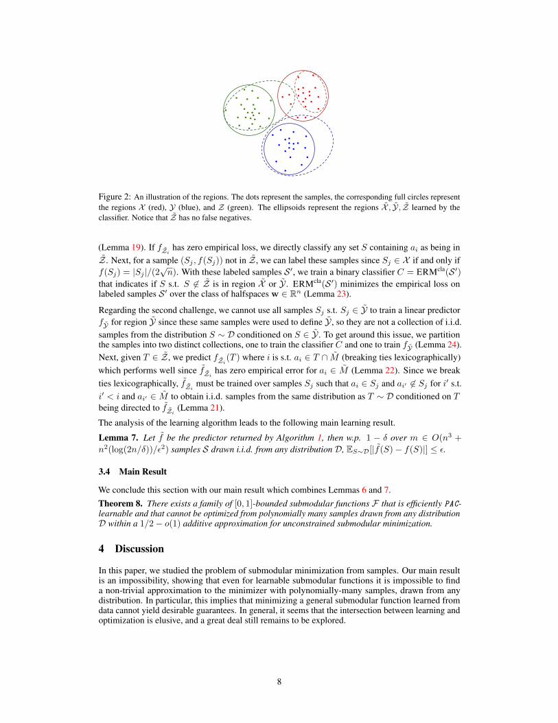
Figure 2: An illustration of the regions. The dots represent the samples, the corresponding full circles representthe regions X (red), Y (blue), and Z (green). The ellipsoids represent the regions X , Y, Z learned by theclassifier. Notice that Z has no false negatives.
(Lemma 19). If fZi has zero empirical loss, we directly classify any set S containing ai as being inZ . Next, for a sample (Sj , f(Sj)) not in Z , we can label these samples since Sj ∈ X if and only iff(Sj) = |Sj |/(2
√n). With these labeled samples S ′, we train a binary classifier C = ERMcla(S ′)
that indicates if S s.t. S 6∈ Z is in region X or Y . ERMcla(S ′) minimizes the empirical loss onlabeled samples S ′ over the class of halfspaces w ∈ Rn (Lemma 23).
Regarding the second challenge, we cannot use all samples Sj s.t. Sj ∈ Y to train a linear predictorfY for region Y since these same samples were used to define Y , so they are not a collection of i.i.d.samples from the distribution S ∼ D conditioned on S ∈ Y . To get around this issue, we partitionthe samples into two distinct collections, one to train the classifier C and one to train fY (Lemma 24).Next, given T ∈ Z , we predict fZi(T ) where i is s.t. ai ∈ T ∩ M (breaking ties lexicographically)which performs well since fZi has zero empirical error for ai ∈ M (Lemma 22). Since we breakties lexicographically, fZi must be trained over samples Sj such that ai ∈ Sj and ai′ 6∈ Sj for i′ s.t.i′ < i and ai′ ∈ M to obtain i.i.d. samples from the same distribution as T ∼ D conditioned on Tbeing directed to fZi (Lemma 21).
The analysis of the learning algorithm leads to the following main learning result.
Lemma 7. Let f be the predictor returned by Algorithm 1, then w.p. 1 − δ over m ∈ O(n3 +
n2(log(2n/δ))/ε2) samples S drawn i.i.d. from any distribution D, ES∼D[|f(S)− f(S)|] ≤ ε.
3.4 Main Result
We conclude this section with our main result which combines Lemmas 6 and 7.Theorem 8. There exists a family of [0, 1]-bounded submodular functions F that is efficiently PAC-learnable and that cannot be optimized from polynomially many samples drawn from any distributionD within a 1/2− o(1) additive approximation for unconstrained submodular minimization.
4 Discussion
In this paper, we studied the problem of submodular minimization from samples. Our main resultis an impossibility, showing that even for learnable submodular functions it is impossible to finda non-trivial approximation to the minimizer with polynomially-many samples, drawn from anydistribution. In particular, this implies that minimizing a general submodular function learned fromdata cannot yield desirable guarantees. In general, it seems that the intersection between learning andoptimization is elusive, and a great deal still remains to be explored.
8

References[Bal15] Maria-Florina Balcan. Learning submodular functions with applications to multi-agent systems. In
Proceedings of the 2015 International Conference on Autonomous Agents and Multiagent Systems,AAMAS 2015, Istanbul, Turkey, May 4-8, 2015, page 3, 2015.
[BH11] Maria-Florina Balcan and Nicholas JA Harvey. Learning submodular functions. In Proceedings ofthe forty-third annual ACM symposium on Theory of computing, pages 793–802. ACM, 2011.
[BRS16] Eric Balkanski, Aviad Rubinstein, and Yaron Singer. The power of optimization from samples. InAdvances in Neural Information Processing Systems, pages 4017–4025, 2016.
[BRS17] Eric Balkanski, Aviad Rubinstein, and Yaron Singer. The limitations of optimization from samples.Proceedings of the Forty-Ninth Annual ACM on Symposium on Theory of Computing, 2017.
[BS17] Eric Balkanski and Yaron Singer. The sample complexity of optimizing a convex function. InCOLT, 2017.
[BVW16] Maria-Florina Balcan, Ellen Vitercik, and Colin White. Learning combinatorial functions frompairwise comparisons. In Proceedings of the 29th Conference on Learning Theory, COLT 2016,New York, USA, June 23-26, 2016, pages 310–335, 2016.
[CLSW16] Deeparnab Chakrabarty, Yin Tat Lee, Aaron Sidford, and Sam Chiu-wai Wong. Subquadraticsubmodular function minimization. arXiv preprint arXiv:1610.09800, 2016.
[DTK16] Josip Djolonga, Sebastian Tschiatschek, and Andreas Krause. Variational inference in mixedprobabilistic submodular models. In Advances in Neural Information Processing Systems 29: AnnualConference on Neural Information Processing Systems 2016, December 5-10, 2016, Barcelona,Spain, pages 1759–1767, 2016.
[EN15] Alina Ene and Huy L. Nguyen. Random coordinate descent methods for minimizing decomposablesubmodular functions. In Proceedings of the 32nd International Conference on Machine Learning,ICML 2015, Lille, France, 6-11 July 2015, pages 787–795, 2015.
[FK14] Vitaly Feldman and Pravesh Kothari. Learning coverage functions and private release of marginals.In COLT, pages 679–702, 2014.
[FKV13] Vitaly Feldman, Pravesh Kothari, and Jan Vondrák. Representation, approximation and learning ofsubmodular functions using low-rank decision trees. In COLT, pages 711–740, 2013.
[FMV11] Uriel Feige, Vahab S. Mirrokni, and Jan Vondrák. Maximizing non-monotone submodular functions.SIAM J. Comput., 40(4):1133–1153, 2011.
[GLS81] Martin Grotschel, Laszlo Lovasz, and Alexander Schrijver. The ellipsoid method and its conse-quences in combinatorial optimization. Combinatorica, 1(2):169–197, 1981.
[IFF01] Satoru Iwata, Lisa Fleischer, and Satoru Fujishige. A combinatorial strongly polynomial algorithmfor minimizing submodular functions. J. ACM, 48(4):761–777, 2001.
[IJB13] Rishabh K. Iyer, Stefanie Jegelka, and Jeff A. Bilmes. Curvature and optimal algorithms for learningand minimizing submodular functions. In Advances in Neural Information Processing Systems 26:27th Annual Conference on Neural Information Processing Systems 2013. Proceedings of a meetingheld December 5-8, 2013, Lake Tahoe, Nevada, United States., pages 2742–2750, 2013.
[JB11] Stefanie Jegelka and Jeff Bilmes. Submodularity beyond submodular energies: coupling edges ingraph cuts. In Computer Vision and Pattern Recognition (CVPR), 2011 IEEE Conference on, pages1897–1904. IEEE, 2011.
[JLB11] Stefanie Jegelka, Hui Lin, and Jeff A Bilmes. On fast approximate submodular minimization. InAdvances in Neural Information Processing Systems, pages 460–468, 2011.
[NB12] Mukund Narasimhan and Jeff A Bilmes. A submodular-supermodular procedure with applicationsto discriminative structure learning. arXiv preprint arXiv:1207.1404, 2012.
[SK10] Peter Stobbe and Andreas Krause. Efficient minimization of decomposable submodular functions.In Advances in Neural Information Processing Systems, pages 2208–2216, 2010.
[SSBD14] Shai Shalev-Shwartz and Shai Ben-David. Understanding machine learning: From theory toalgorithms. Cambridge university press, 2014.
9

A Optimization from Samples via Learning then Optimization
In this section, we discuss the issues with the approach which consists of first learning a surrogateof the true function and then optimizing this surrogate. A first issue is that the surrogate may benon-submodular, and even though we might be able to approximate the true function everywhere,the surrogate may be intractable to optimize (Section A.1). A second issue is that the surrogate issubmodular and approximates the true function on all the samples but that its minimum is far fromthe minimum of the true function (Section A.2).
A.1 The surrogate is a good approximation of the true function but is not submodular
Consider the following submodular function defined over a partition of the ground set N into a set ofgood elements G and a set of bad elements B, each of size n/2:
f(S) =1
2+
1
n(|S ∩B| − |S ∩G|) .
Let f be a surrogate for f defined as follows:
f(S) =1
2+
1n (|S ∩B| − |S ∩G|) if ||S ∩B| − |S ∩G|| ≥ 1
2εn
0 otherwise
It is easy to verify that the surrogate f ε-approximates f on all sets. However f is intractable tooptimize. Intuitively, by concentration bounds, a query S of the algorithm has value f(S) = 1/2for an exponentially high fraction of the sets S. Thus, with polynomially many adaptive queries(S, f(S)) of the choice of the algorithm, the algorithm will probably not be able to distinguish f(S)from the constant function 1/2 everywhere. Since the optimal solution is S? = G and has value 0,no algorithm can then do better than the trivial 1/2-approximation to minimize f .
A.2 The surrogate is submodular but its minimum is far from the true minimum
We illustrate the second issue with samples from the uniform distribution. Similarly, consider thefollowing submodular function defined over a partition of the ground setN into a set of good elementsG and a set of bad elements B, each of size n/2
f(S) :=
1
2+
1
2n· (|S ∩G|+ |S ∩B|) if |S ∩G| < n/2
1
2n· |S ∩B| if |S ∩G| = n/2
This function is similar to the functions constructed in Section 2. Let f be a surrogate for f where Gand B are interchanged:
f(S) :=
1
2+
1
2n· (|S ∩B|+ |S ∩G|) if |S ∩B| < n/2
1
2n· |S ∩G| if |S ∩B| = n/2
It is easy to verify that given polynomially many samples S from the uniform distribution, f(S) =f(S) with high probability, so f is consistent with all the samples. However its minimum B, whichis such that f(B) = 0 is a bad solution for the true underlying function since f(B) = 3/4.
B Concentration bounds
Lemma 9 (Chernoff Bound). Let X1, . . . , Xn be independent indicator random variables. LetX =
∑ni=1Xi and µ = E[X]. For 0 < δ < 1,
Pr[|X − µ| ≥ δµ] ≤ 2e−µδ2/3.
10

B.1 Concentration bounds from Section 2
• Every set Si in the sample respects |Si| ≤ 3n/4, w.p. 1−e−Ω(n). Consider a set Si ∼ U . LetXj be an indicator variable indicating if j ∈ Si. By Chernoff bound with |S| =
∑nj=1Xj ,
µ = n/2, δ = 1/2, Pr[|Si| − n/2 ≥ n/4] ≤ 2e−n/24. By a union bound over allpolynomially many samples, the claim holds with probability 1− e−Ω(n).
• For sets S1, . . . , Sm, m = poly(n), all of size at most 3n/4, when fj is drawn u.a.r.from F we get that |Si ∩ Gj | <
√n, w.p. 1 − e−Ω(n1/2). Consider a set T of size
n/4. Let X1, . . . , Xn/4 be indicator variables indicating if elements in T are also in Gj .By Chernoff bound with |T ∩ Gj | =
∑n/4i=1 Xi, µ = n/4 ·
√n/n =
√n/4, δ = 1/2,
Pr[|T ∩ Gj | −√n/4 ≥
√n/8] ≤ 2e−n
1/2/48. Thus, with probability 1 − e−Ω(n1/2),|T ∩Gj | > 0, and for a set S of size at most 3n/4, |(N \ S) ∩Gj | > 0 and Gj 6⊆ S. Thus,by a union bound, it holds with probability 1 − e−Ω(n1/2) over fj that for all samples S,Gj 6⊆ S.
• Fix S and choose f u.a.r. from F , then, w.p. 1− e−Ω(n1/6):
f(S) ≥ 1
2− o(1).
If |S| ≤ n − n2/3, let T ⊆ N \ S such that |T | = n2/3. Let X1, . . . , Xn2/3 be indicatorvariables indicating if elements in T are also in G. By Chernoff bound with |T ∩ G| =∑n2/3
i=1 Xi, µ = n2/3 ·√n/n = n1/6, δ = 1/2, Pr[|T ∩G|−n1/6 ≥ n1/6/2] ≤ 2e−n
1/6/12.Thus, with probability 1− e−Ω(n1/6), |T ∩G| > 0 and |S ∩G| <
√n. Thus, f(S) ≥ 1/2.
If |S| > n − n2/3, then f(S) ≥ (n − 2n2/3)/(2n) = n(1 − o(1))/(2n(1 − o(1))) =(1− o(1))/2.
B.2 Concentration bounds from Section 3
• For all S ⊆ N such that |S| ≥ n1/4, with probability 1 − e−Ω(n1/4) over FM , we have|M ∩ S| ≥ 1. Let Xi, for i ∈ S, indicate if i ∈ M . With µ = |S|(n/2 −
√n)/n and
δ = 1/2,
Pr
[∣∣∣∣M ∩ S| − |S| · n/2−√nn
∣∣∣∣ ≥ |S| · n/2−√n2n
]≤ 2e−n
1/4·n/2−√n
12n = e−Ω(n1/4).
Thus, |M ∩ S| ≥ 1 with probability at least 1− e−Ω(n1/4).
• Let S ⊆ N and fi ∈ FM such that m = 0, |S| ≥ n3/4, and S independent of i, then
(1− o(1)) · |S| ≤ n/2 +√n√
n· b, n/2 +
√n
n/2· g ≤ (1 + o(1)) · |S|.
Let Xj , for j ∈ S, indicate if j ∈ Bi. With µ = |S|(√n/(n/2 +
√n)) and δ = n−1/16,
Pr
[∣∣∣∣g − √n
n/2 +√n· |S|
∣∣∣∣ ≥ n−1/16 ·√n
n/2 +√n· |S|
]≤ 2e
−n−1/8·√n
3(n/2+√n)·n7/8
= e−Ω(n1/4)
Similarly,
Pr
[∣∣∣∣g − n/2
n/2 +√n· |S|
∣∣∣∣ ≥ n−1/16 · n/2
n/2 +√n· |S|
]≤ 2e
−n−1/8· n/2
3(n/2+√n)·n7/8
= e−Ω(n3/4)
and we obtain the desired result.
11
C Missing analysis from Sections 3.1 and 3.2
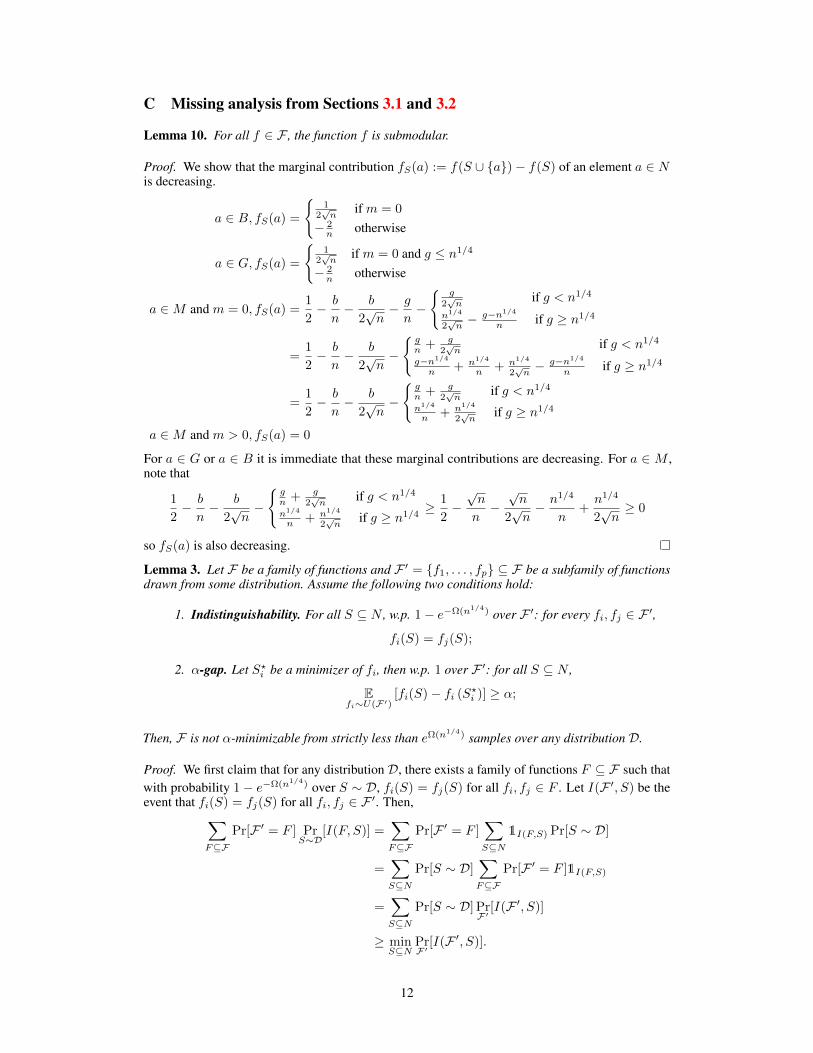
Lemma 10. For all f ∈ F , the function f is submodular.
Proof. We show that the marginal contribution fS(a) := f(S ∪ a)− f(S) of an element a ∈ Nis decreasing.
a ∈ B, fS(a) =
1
2√n
if m = 0
− 2n otherwise
a ∈ G, fS(a) =
1
2√n
if m = 0 and g ≤ n1/4
− 2n otherwise
a ∈M and m = 0, fS(a) =1
2− b
n− b
2√n− g
n−
g
2√n
if g < n1/4
n1/4
2√n− g−n1/4
n if g ≥ n1/4
=1
2− b
n− b
2√n−
gn + g
2√n
if g < n1/4
g−n1/4
n + n1/4
n + n1/4
2√n− g−n1/4
n if g ≥ n1/4
=1
2− b
n− b
2√n−
gn + g
2√n
if g < n1/4
n1/4
n + n1/4
2√n
if g ≥ n1/4
a ∈M and m > 0, fS(a) = 0
For a ∈ G or a ∈ B it is immediate that these marginal contributions are decreasing. For a ∈ M ,note that
1
2− b
n− b
2√n−
gn + g
2√n
if g < n1/4
n1/4
n + n1/4
2√n
if g ≥ n1/4≥ 1
2−√n
n−√n
2√n− n1/4
n+n1/4
2√n≥ 0
so fS(a) is also decreasing.
Lemma 3. Let F be a family of functions and F ′ = f1, . . . , fp ⊆ F be a subfamily of functionsdrawn from some distribution. Assume the following two conditions hold:
1. Indistinguishability. For all S ⊆ N , w.p. 1− e−Ω(n1/4) over F ′: for every fi, fj ∈ F ′,
fi(S) = fj(S);
2. α-gap. Let S?i be a minimizer of fi, then w.p. 1 over F ′: for all S ⊆ N ,
Efi∼U(F ′)
[fi(S)− fi (S?i )] ≥ α;
Then, F is not α-minimizable from strictly less than eΩ(n1/4) samples over any distribution D.
Proof. We first claim that for any distribution D, there exists a family of functions F ⊆ F such thatwith probability 1− e−Ω(n1/4) over S ∼ D, fi(S) = fj(S) for all fi, fj ∈ F . Let I(F ′, S) be theevent that fi(S) = fj(S) for all fi, fj ∈ F ′. Then,∑
F⊆F
Pr[F ′ = F ] PrS∼D
[I(F, S)] =∑F⊆F
Pr[F ′ = F ]∑S⊆N
1I(F,S) Pr[S ∼ D]
=∑S⊆N
Pr[S ∼ D]∑F⊆F
Pr[F ′ = F ]1I(F,S)
=∑S⊆N
Pr[S ∼ D] PrF ′[I(F ′, S)]
≥ minS⊆N
PrF ′[I(F ′, S)].
12

Thus, there exists some F = f1, . . . , fp such thatPrS∼D
[I(F, S)] ≥ minS⊆N
PrF ′[I(F ′, S)].
Since minS⊆N PrF ′ [I(F ′, S)] = 1− e−Ω(n1/4). Then, by a union bound over the samples, fi(S) =fj(S) for all fi, fj ∈ F and for all samples S with probability 1− e−Ω(n1/4), and we assume this isthe case, as well as the gap condition, for the remaining of the proof.
It follows that the choices of the algorithm given samples from fi, i ∈ [p], are independent of i.Pick i ∈ [p] uniformly at random and consider the (possibly randomized) vector S returned by thealgorithm. Since S is independent of i and by the α-gap condition,
Efi∼U(F ′)
[fi(S)− fi (S?i )] ≥ α.
Thus, there exists at least one fi ∈ F such that for fi, the algorithm is at least an additive factor αaway from fi(S
?i ).
D Missing analysis from Section 3.3
We begin by reviewing known results for classification and linear regression using the VC-dimensionand the Rademacher complexity (Section D.1) and then give the missing analysis for the learningalgorithm (Section D.2).
D.1 VC-dimension and Rademacher complexities essentials
We review learning results needed for the analysis. These results use the VC-dimension and theRademacher complexity, two of the most common tools to bound the generalization error of a learningalgorithm. We formally define the VC-dimension and the Rademacher complexity using definitionsfrom [SSBD14]. We begin with the VC-dimension, which is for classes of binary functions. Wefirst define the concepts of restriction to a set and of shattering, which are useful to define theVC-dimension.Definition 11. (Restriction of H to A). Let H be a class of functions from X to 0, 1 and letA = a1, . . . , am ⊂ X . The restriction ofH to A is the set of functions from A to 0, 1 that canbe derived fromH. That is,
HA = (h(a1), . . . , h(am)) : h ∈ H,where we represent each function from A to 0, 1 as a vector in 0, 1|A|.Definition 12. (Shattering). A hypothesis classH shatters a finite set A ⊂ X if the restriction ofHto A is the set of all functions from A to 0, 1. That is, |HA| = 2|A|.Definition 13. (VC-dimension). The VC-dimension of a hypothesis classH is the maximal size of aset S ⊂ X that can be shattered byH. IfH can shatter sets of arbitrarily large size we say thatHhas infinite VC-dimension.
Next, we define the Rademacher complexity, which is for more complex classes of functions thanbinary functions, such as real-valued functions.Definition 14. (Rademacher complexity). Let σ be distributed i.i.d. according to Pr[σi = 1] =Pr[σi = −1] = 1/2. The Rademacher complexity R(A) of set of vectors A ⊂ Rm is defined as
R(A) :=1
mEσ
[supa∈A
m∑i=1
σiai
].
This first result bounds the generalization error of a class of binary functions in terms of the VC-dimension of these classifiers.Theorem 15 ([SSBD14]). LetH be a hypothesis class of functions from a domain X to −1, 1 andf : X 7→ −1, 1 be some “correct" function. Assume that the VC-dimension ofH is d. Then, thereis an absolute constant C such that with m ≥ C(d+ log(1/δ))/ε2 i.i.d. samples x1, . . . ,xm ∼ D,∣∣∣∣∣ PrS∼D
[h(S) 6= f(S)]− 1
m
m∑i=1
1h(Si)6=f(Si)
∣∣∣∣∣ ≤ εfor all h ∈ H, with probability 1− δ over the samples.
13

We use the class of halfspaces for classification, for which we know the VC-dimension.Theorem 16 ([SSBD14]). Let b ∈ R. The class of functions x 7→ sign(wᵀx) + b : w ∈ Rn hasVC dimension n.
The following result combines the generalization error of a class of functions in terms of itsRademacher complexity with the Rademacher complexity of linear functions over a ρ-Lipschitz lossfunction.Theorem 17 ([SSBD14]). Suppose that D is a distribution over X such that with probability1 over x ∼ D we have that ‖x‖∞ ≤ R. Let H = w ∈ Rd : ‖w‖1 ≤ B and let`(w, (x, y)) = φ(wᵀx, y) such that for all y ∈ Y , a 7→ φ(a, y) is an ρ-Lipschitz function andsuch that maxa∈[−BR,BR] |φ(a, y)| ≤ c. Then, for any δ ∈ (0, 1), with probability of at least 1− δover the choice of an i.i.d. sample of size m,
Ex∼D
[|`(w, (x, y))|] ≤ 1
|S|∑x∈S|`(w, (x, y))|+ 2ρBR
√2 log(2d)
m+ c
√2 log(2/δ)
m
for all w ∈ H.
D.2 Missing analysis for the learning algorithm
We formally define PAC learnability with absolute loss.Definition 18 (PAC learnability with absolute loss). A class of functions F is PAC learnable if thereexist a function mF : (0, 1)2 → N and a learning algorithm with the following property: Forevery ε, δ ∈ (0, 1), for every distribution D, and every function f ∈ F , when running the learningalgorithm on m ≥ mH(ε, δ) i.i.d. samples (S, f(S)) with S ∼ D, the algorithm returns a function fsuch that, with probability at least 1− δ (over the choice of the m training examples),
ES∼D
[∣∣∣f(S)− f(S)∣∣∣] ≤ ε.For the remaining of this section, let f ∈ F be the function defined over partition (G,B,M) for whichthe learning algorithm is given samples S . Let xS denote the 0− 1 vector corresponding to the set S,i.e., xi = 1i∈S . We define the following subcollection of samples, SZi := (S, f(S)) ∈ S : S ∈ Zi,S≤X∪Y := (Sj , f(Sj)) ∈ S : Sj 6∈ Z, j ≤ m/2, S>Y := (Sj , f(Sj)) ∈ S : Sj ∈ Y, j > m/2.Let R be a region of sets, we define DR to be the distribution S ∼ D conditioned on S ∈ R. Thelinear regression predictors fZi and fY and the classifier C are formally defined as follows.
wi := argminw∈Rn:‖w‖1≤1
∑(Sj ,f(Sj))∈SZi
|wᵀxS + 1− f(S)|
wC := argminw∈Rn
∑(Sj ,f(Sj))∈S≤X∪Y
1sign(wᵀxS+n1/4)=sign(f(S)−|S|/(2√n))
wY := argminw∈Rn:‖w‖1≤1
∑(Sj ,f(Sj))∈S>Y
|wᵀxS + bY − f(S)|
where bY is the constant bY = 1/2 + 1/(2n1/4) + 1/n3/4. Then,
fZi(S) := wᵀi · xS + 1
C(S) := sign(wᵀCxS + n1/4
)fY(S) := wᵀ
Y · xS + bY
We show that there are no false negatives for Z, which is important for the existence of a linearclassifier C with zero empirical error on samples S≤
X∪Y .
Lemma 19. If S 6∈ Z , then S ∈ X ∪ Y .
14

Proof. The proof is by contrapositive. If S 6∈ X ∪ Y , then there exists i ∈ M such that i ∈ S.Then note that f(S) is an affine function over all S such that i ∈ S. So it must be the case that theempirical minimizer wi computed has zero empirical loss. Thus i ∈ M .
We give a general lemma for the expected error of a linear regression predictor.
Lemma 20. Assume S ′ is a collection of m ≥ ε−2(log(2n) + log(2/δ))/2 i.i.d. samples from somedistribution D′. Then, with probability at least 1− δ,
ES∼D′
[|wᵀxS + b− f(S)|] ≤ 1
|S ′|∑S∈S′
|wᵀxS + b− f(S)|+ ε
for all w ∈ Rn such that ||w||1 ≤ 1.
Proof. Consider the setting of Theorem 17 with the absolute loss, so `(w, (xS , f(S)) =φ(wᵀxS , f(S)) = |wᵀxS + b− f(S)| for some b ∈ R. Notice that the absolute loss is 1-Lipschitz,so ρ = 1. We also have d = n and ‖xS‖∞ ≤ 1 = R for all S. We consider ‖w‖1 ≤ 1 = B.Such B and R imply that c = 2 satisfies the condition of Theorem 17. Thus, if S ′ is a set ofm ≥ ε−2(log(2n) + log(2/δ))/2 i.i.d. samples from a distribution D′, then with probability at least1− δ,
ES∼D′
[|wᵀxS + b− f(S)|] ≤ 1
|S ′|∑S∈S′
∣∣wᵀYxS + b− f(S)
∣∣+ ε
for all w ∈ Rn such that ||w||1 ≤ 1.
We show that if S ∈ Zi with i ∈ M , then the learner f directs S to fZi .
Lemma 21. Assume S ∈ Zi, with i ∈ M . Then, f(S) = fZi(S)
Proof. We argue that i = min(i′ : i ∈ S ∩ M). Assume by contradiction that there exists i′ < i
such that i′ ∈ S ∩ M . Then it must be the case that S ∈ Z before iteration i of the algorithm. Butthen, S would not have been considered for Zi.
The following lemma bounds the error of linear regression predictors fZi with i ∈ M .
Lemma 22. Assume |SZi | ≥ ε−2(log(2n) + log(2/δ))/2 and i ∈ M . Then with probability 1− δ
over SZi ,
ES∼DZi
[∣∣∣f(S)− f(S)∣∣∣] = ES∼DZi
[|wᵀi xS + 1− f(S)|] ≤ ε.
Proof. By Lemma 21,
ES∼DZi
[∣∣∣f(S)− f(S)∣∣∣] = ES∼DZi
[|wᵀi xS + 1− f(S)|]
Let i ∈ M , then, the empirical loss of wi is zero, i.e.,∑S∈Si |w
ᵀi xS + 1− f(S)| = 0 by Algo-
rithm 1 since i ∈ M . The collection of samples SZi consists of m i.i.d. samples S from DZi , so byLemma 20,
ES∼DZi
[|wᵀi xS + 1− f(S)|] ≤ ε.
Next, we bound the error of classifier C.
Lemma 23. Assume |S≤X∪Y | ≥ C(n+ log(1/δ))/ε2. Then, with probability 1− δ over S≤X∪Y ,
PrS∼DX∪Y
[sign
((wC)
ᵀxS + n1/4
)= sign (S ∈ X )
]≤ ε.
15

Proof. Note that the support of DX∪Y does not contain any set S ∈ Z by Lemma 19. Thus we onlyconsider S ∈ X ∪ Y for the remaining of the analysis. Consider the classifier
h?(S) = sign((w?)
ᵀxS + n1/4
)where w?i = −1 if i ∈ G and w?i = 0 otherwise. Then h?(S) = 1 if S ∈ X and h?(S) = −1 ifS ∈ Y . Since w? has zero empirical error over S≤X∪Y , it must also be the case for the empirical riskminimizer wC , ∑
(S,f(S))∈S≤X∪Y
1sign((wC)ᵀxS+n1/4)=sign(S∈X ) = 0.
By Theorem 16, the class of functions S 7→ sign(wᵀx+ n1/4) : w ∈ Rn has VC dimension n.Since S≤X∪Y is a collection of i.i.d. samples S from DX∪Y , we conclude by Theorem 15 that with
probability 1− δ over S≤X∪Y ,
PrS∼DX∪Y
[sign
((wC)
ᵀxS + n1/4
)= sign (S ∈ X )
]≤ ε
with |S≤X∪Y | ≥ C(n+ log(1/δ))/ε2.
We bound the error of the linear regression predictor wY . Note the additional|S>Y∩X||S>Y| term that is due
the predictor being trained over S>Y which might contain samples in X which have been misclassified
in Y .Lemma 24. Assume |S>Y | ≥ ε
−2(log(2n) + log(2/δ))/2. Then with probability 1− δ over S>Y ,
ES∼DY
[∣∣∣wᵀYxS + bY − f(S)
∣∣∣] ≤ ε+ |S>Y ∩ X ||S>Y |.
Proof. Consider the affine function (wY , b) over all sets in region Y . This function has empiricalloss:
1
|S>Y |∑
(S,f(S))∈S>Y
∣∣wᵀYxS + bY − f(S)
∣∣
=1
|S>Y |
∑(S,f(S))∈S>
Y:S∈X
∣∣wᵀYxS + bY − f(S)
∣∣+ ∑(S,f(S))∈S>
Y:S∈Y
∣∣wᵀYxS + bY − f(S)
∣∣
≤ 1
|S>Y |
(|S>Y ∩ X |+ 0
)=|S>Y ∩ X ||S>Y |
Since wY is the empirical loss minimizer, it has smaller empirical loss than wY , so∑(S,f(S))∈S>
Y
∣∣∣wᵀYxS + bY − f(S)
∣∣∣ ≤ |S>Y ∩X||S>Y| .
Since S>Y consists of m i.i.d. samples from DY (in particular, none of these samples were used totrain classifier C) and by Theorem 20, we conclude that
ES∼DY
[∣∣∣wᵀYxS + bY − f(S)
∣∣∣] ≤ ε+ |S>Y ∩ X ||S>Y |.
16

We show a general lemma to analyze the cases where the linear predictors are trained over a smallnumber of samples.Lemma 25. Let S be the collection of m i.i.d. samples drawn from D. Assume m ≥ 12
ε log(2/δ)and let S ′ ⊆ S, then it is either the case that
PrS∼D
[S ∈ S ′] ≤ ε
or|S ∩ S ′| ≥ εm
2with probability at least 1− δ.
Proof. By Chernoff bound with µ = εm and m ≥ 12ε log(2/δ):
PrS[|S ∩ S ′| − εm| ≥ εm/2] ≤ 2e−εm/12 ≤ δ
We bound the additional|S>Y∩X||S>Y| term from Lemma 24 in the case where the number of samples S>Y
is large enough.Lemma 26. Assume |S>Y | ≥ 12n2 log(2n/δ)/ε2, then
|S>Y ∩ X ||S>Y |
≤ 3
2Pr
S∼DY[S ∈ X ] + 3ε
2n
with probability 1− δ/n
Proof. If PrS∼DY [S ∈ X ] ≥ ε/n, then by the Chernoff bound:
Pr
[||S>Y ∩ X | − |S
>Y | Pr
S∼DY[S ∈ X ] | ≥ 1
2Pr
S∼DY[S ∈ X ] |S>Y |
]≤ 2e
−|S>Y|PrS∼DY
[S∈X ]/12
≤ 2e−|S>Y|ε/(12n)
and |S>Y ∩X | ≤32 |S
>Y |PrS∼DY [S ∈ X ] with probability 1− δ/n since |S>Y | ≥ 12n2 log(2n/δ)/ε2.
Otherwise, by another Chernoff bound:
Pr
[||S>Y ∩ X | − |S
>Y | Pr
S∼DY[S ∈ X ] | ≥ ε
2n· |S>Y |
]=Pr
[||S>Y ∩ X | − |S
>Y | Pr
S∼DY[S ∈ X ] | ≥ 1
2n
ε
PrS∼DY [S ∈ X ]· |S>Y | Pr
S∼DY[S ∈ X ]
]
≤2e−|S>Y|PrS∼DY
[S∈X ]( 12n
εPrS∼DY
[S∈X ])2/3
≤2e−|S>
Y|ε2/(12n2)
and since PrS∼DY [S ∈ X ] ≤ ε/n, |S>Y ∩ X | ≤ 3|S>Y |ε/(2n) with probability 1 − δ/n since|S>Y | ≥ 12n2 log(2n/δ)/ε2
We are now ready to put all the pieces together and show the main result for the learning algorithm.
Lemma 7. Let f be the predictor returned by Algorithm 1, then w.p. 1 − δ over m ∈ O(n3 +
n2(log(2n/δ))/ε2) samples S drawn i.i.d. from any distribution D, ES∼D[|f(S)− f(S)|] ≤ ε.
Proof. Let `(S) =∣∣∣f(S)− f(S)∣∣∣ be the loss by the algorithm. We divide the analysis in three cases
dependent on which region S ∼ D falls into.
ES∼D
[`(S)] = PrS∼D
[S ∈ X ] ES∼DX
[`(S)]+ PrS∼D
[S ∈ Y] ES∼DY
[`(S)]+∑i∈M
PrS∼D
[S ∈ Zi] ES∼DZi
[`(S)]
17

We analyze each of these three cases separately. Note that since f(S) ∈ [0, 1] and since all the linearregression predictors w have bounded norm ‖w‖1 ≤ 1, `(S) ≤ 2.
If S ∈ X . Then, S 6∈ Z by Lemma 19. Thus it is either the case that S ∈ X or S ∈ Y . We getE
S∼DX[`(S)] = Pr
S∼DX[S ∈ X ] E
S∼DX∩X[`(S)] + Pr
S∼DX[S ∈ Y] E
S∼DX∩Y[`(S)]
≤ 1 · ES∼DX∩X
[|S|2√n− |S|
2√n
]+ PrS∼DX
[S ∈ Y] · 2
≤ 2 PrS∼DX
[S ∈ Y]
If S ∈ Y . Then, if PrS∼D[S ∈ Y] ≤ ε/(2n),
PrS∼D
[S ∈ Y] ES∼DY
[`(S)] ≤ ε
n
Otherwise, by Lemma 25, |S>Y | ≥ εm/(4n) ≥ (n/ε)2 log(2n/δ), so by Lemma 24, with probabilityat least 1− δ/n,
PrS∼D
[S ∈ Y] ES∼DY
[`(S)] ≤ ε
n+ PrS∼D
[S ∈ Y]
(|S>Y ∩ X ||S>Y |
)
If S ∈ Zi. Then if PrS∼D [S ∈ Zi] ≤ ε/(4n),
PrS∼D
[S ∈ Zi] ES∼Di
[`(S)] ≤ ε
2n.
Otherwise, by Lemma 25 |Si| ≥ εm/(8n) ≥ (2n/ε)2 log(2n/δ), so by Lemma 22, with probabilityat least 1− δ/n,
PrS∼D
[S ∈ Zi] ES∼Di
[`(S)] ≤ ε
2n.
Combining the three cases, and by a union bound over the at most n events with probability at least1− δ/n, we have that with probaiblity at least 1− δ,
ES∼D
[`(S)]
= PrS∼D
[S ∈ X ] ES∼DX
[`(S)] + PrS∼D
[S ∈ Y] ES∼DY
[`(S)] +∑i∈M
PrS∼D
[S ∈ Zi] ES∼DZi
[`(S)]
≤2 · PrS∼D
[S ∈ X ] PrS∼DX
[S ∈ Y] + PrS∼D
[S ∈ Y]
[ε
n+|S>Y ∩ X ||S>Y |
]+ n · ε
2n
≤2 · PrS∼D
[S ∈ X ] PrS∼DX
[S ∈ Y] + PrS∼D
[S ∈ Y][ε
n+
3
2Pr
S∼DY[S ∈ X ] + 3ε
2n
]+ε
2
≤2 · PrS∼D
[S ∈ X ∪ Y] PrS∼DX∪Y
[S ∈ (X ∩ Y) ∪ (Y ∩ X )] + 3ε
4
where the third inequality is by Lemma 26. If PrS∼D[S ∈ X ∪ Y] ≤ εn ,
PrS∼D
[S ∈ X ∪ Y] PrS∼DX∪Y
[S ∈ (X ∩ Y) ∪ (Y ∩ X )] ≤ ε
n.
Otherwise, by Lemma 25, |S≤X∪Y | ≥ εm/2n ≥ c1(n3 + n2 log(n/δ))/ε2 with probability 1− δ/n,
so by Lemma 23,
PrS∼DX∪Y
[S ∈ (X ∩ Y) ∪ (Y ∩ X )] = PrS∼DX∪Y
[sign ((wC)ᵀxS + nε) 6= sign (S ∈ X )] ≤ ε
n.
and we conlude thatE
S∼D
[∣∣∣f(S)− f(S)∣∣∣] ≤ εwith probability 1− δ.
18