HAL Id: hal-01629988https://hal.archives-ouvertes.fr/hal-01629988

Preprint submitted on 7 Nov 2017

HAL is a multi-disciplinary open accessarchive for the deposit and dissemination of sci-entific research documents, whether they are pub-lished or not. The documents may come fromteaching and research institutions in France orabroad, or from public or private research centers.

L’archive ouverte pluridisciplinaire HAL, estdestinée au dépôt et à la diffusion de documentsscientifiques de niveau recherche, publiés ou non,émanant des établissements d’enseignement et derecherche français ou étrangers, des laboratoirespublics ou privés.

Minimum Age Regulation and Child Labor: NewEvidence from Brazil

Olivier Bargain, Delphine Boutin

To cite this version:Olivier Bargain, Delphine Boutin. Minimum Age Regulation and Child Labor: New Evidence fromBrazil. 2017. �hal-01629988�

Minimum Age Regulation and Child Labor:

New Evidence from BrazilOlivier Bargain and Delphine Boutin

LAREFI Working Paper N°2017-02

https://larefi.u-bordeaux.fr/

LAREFI Université de Bordeaux

Bâtiment Recherche Economie – 1er étage Avenue Léon Duguit – 33 608 Pessac

NOTICES LAREFI Working Papers contain preliminary material and research results. They have been peer reviewed. They are circulated in order to stimulate discussion and critical comment; any opinions expressed are only those of the author(s). Copyright LAREFI. All rights reserved. Sections of this material may be reproduced for personal and not-for-profit use without the express written permission of but with acknowledgment to LAREFI. To reproduce the material contained herein for profit or commercial use requires express written permission. To obtain permission, contact LAREFI at cyril.mesmer@u-bordeaux.fr.

�Acknowledgement: Bargain is a¢ liated with Bordeaux University, the �Institut Universitaire de France� and IZA;

Boutin with Université d�Auvergne, CERDI and IZA. Corresponding author: Olivier Bargain, LAREFI, rue Leon Duguit, 33608 Pessac, France, olivier.bargain@u-bordeaux.fr

LAREFI – LABORATOIRE D’ANALYSE ET DE RECHERCHE EN ECONOMIE ET FINANCES INTERNATIONALES

AUTHORS Olivier Bargain and Delphine Boutin *

Minimum Age Regulation and Child Labor:New Evidence from Brazil

Olivier Bargain and Delphine Boutin

November 6, 2017

Abstract

We suggest new evidence on minimum age regulations using a natural experiment. In 1998, a constitutional reform has changed the minimum working age from 14 to 16 in Brazil. The reform was the legislative counterpart of a broad set of measures taken by a government strongly committed to �ghting child labor. We document the fact that enforcement and compliance may have been heterogeneous across regions and job types. The setting allows improving upon past approaches based on the comparison of employment rates of children below and above the minimum age. Precisely, we observe 14-year old children the year after the reform and exploit discontinuous treatment depending on their birthdate (only those who turned 14 after mid-December 1998 are banned). Regression discontinuity and di¤erence-in-discontinuity designs show no e¤ect of the ban overall, nor a reallocation towards less visible activities, or a substitution of labor within families. Importantly, however, we �nd a signi�cant drop in child labor among those with highest chances of compliance, namely children in visible activities and in regions characterized with an above-average intensity of labor inspections. We provide power calculation and extensive sensitivity checks.

Key Words : child labor, ban, minimum working age, Brazil, regression discontinuity, di¤erence in discontinuity.

JEL Classi�cation : J08, J22, J23, J88.

1 Introduction

Child labor bans in the form of minimum legal age of employment exist in most countries in

the world. In principle, these regulations could decrease child labor if applied uniformly across

di¤erent types of activities. In practice, they may lead to a reallocation of child labor towards

unregulated sectors (like family businesses) where they are not applied or where detection is

hard to enforce. Overall, there is little evidence that minimum age of employment regulations

have any e¤ect at all, and in particular that they are in�uencing child engagement in paid

employment (Edmonds and Shrestha, 2012). There are two main reasons for this observation.

First, it seems that minimum age regulations are not enforced in general. Some of the evidence

stems from historical data on the US (see Manacorda, 2006, for evidence and references therein).

These studies have found a correlation between the adoption of child labor laws in US states and

employment in manufacturing, but the laws tended to follow declines in child labor rather than

to lead them. Similar conclusions are obtained in the di¤erent context of modern minimum

age laws. These laws, passed in many poor countries where child labor is prevalent, seem to be

motivated by global political concerns rather than genuine intentions �and are rarely followed

by appropriate enforcing actions.1 The second reason for seemingly ine¤ective minimum age

laws is the possible di¢ culty to detect an e¤ect. Standard approaches rely on an �age trend�

approach, i.e. a comparison of child employment rates around the minimum legal age, that

may not be precise enough to reveal a potential e¤ect of minimum age legislations (Edmonds,

2014).

Against this background, we suggest new evidence based on a change in the Brazilian law. On

the 15th of December 1998, the minimum legal age for work was increased from 14 to 16. We

�rst show that the reform corresponded to a real intention of the Brazilian government to make

it work. Indeed, the law involved a change in the Constitution and, anticipating the rati�cation

of ILO minimum age conventions, was also part of a broad set of measures intended to eradicate

child labor in Brazil. Moreover, its enforcement could �nd support on an operational system

of labor inspections that refocused on the detection of illegal labor among children at that

period. We nonetheless document the fact that enforcement and compliance may have been

heterogeneous across regions and job types.

Secondly, we suggest an empirical approach that is more precise than previous methods to detect

potential e¤ects of the reform. Indeed, the literature tends to compare employment rates of

children below and above the minimum age, while it is di¢ cult to control for underlying age

1They are typically based on the principles of the International Labour Organization�s minimum age con-

ventions, i.e. Convention C138 on the Minimum Age of Employment and C182 on the Worst Forms of Child

Labor. Boockmann (2010) �nds little evidence that ILO conventions increase school attendance or decrease

child labor.

1

trends in employment. In our setting, the reform lends itself to discontinuity-based approaches

to extract a causal e¤ect of the ban. Precisely, the new ban a¤ected those who turned 14 years

old after mid-December 1998 but not those who turned 14 before. Using the Pesquisa Nacional

por Amostra de Domicilios (PNAD), we observe these children in September 1999, when they

are all aged 14. With regression discontinuity designs (RD), we exploit the discontinuous

eligibility for work of these children depending on their birthdate. In di¤erence-in-discontinuity

(DDisc), we combine discontinuous treatment and the time change around the threshold.

Our results can be summarized as follows. Both RD and DDisc estimations point to the absence

of an overall e¤ect of the new ban on children around 14 years of age. We also �nd no sign of

a reallocation from "visible" �rms towards activities that more easily escape inspections (like

home-based or outdoor work), nor a substitution of labor within families. Results are robust

to extensive sensitivity checks and are not due to a lack of statistical power. Importantly,

heterogenous estimations point to a signi�cant drop in child labor among those with highest

chances of compliance, namely children in visible activities and in regions characterized by

an above-average intensity of labor inspections. We discuss these results in the context of a

relatively small literature using natural experiments to identify the potential e¤ect of child

labor bans.2

2 Background

2.1 Mininum Age Regulation in the Literature

Minimum age of employment regulations have been one of the most used tools worldwide to

combat child labor. Therefore, they have received lots of attention in the theoretical literature

on child labor.3 In the seminal paper of Basu and Van (1998), there is only one sector of

employment for child labor so that a ban can completely prohibit it. Basu (2005) adds a

second, unregulated sector. In a two-sector model, enforced minimum age regulations can

divert children from regulated activities to non-regulated activities rather than eliminating

child employment. In fact, the rise in labor costs to employers induces a lower demand in

child labor and lower child wages (an equivalent result is obtained if employers recoup the risk

premium by reporting these costs on children wages). Overall child labor may even increase

if depressed wages lead budget-constrained households to send more children to work.4 This

2The closest study to ours is Bharadwaj et al. (2013), who exploit changes in the minimum working age in

India (see section 2).3This literature includes early contributions by Basu and Van (1998), Ranjan (1999), Baland and Robinson

(2000), Dessy (2000), Basu (2005), and Dessy and Pallage (2005).4See Edmonds (2008) for a review of the links between household poverty and child labor.

2

may also happen if children shifted away from the regulated sector now work in family business

and no longer bring external resources. Edmonds and Shrestha (2012) de�ne three necessary

conditions for the sector reallocation following a ban in the regulated sector to be neutral

on overall child employment: "adults" (i.e. parents or siblings above the minimum age) can

move freely between the household and the regulated sector (competitive adult labor markets);

adults and children are perfect substitutes subject to a productivity shifter (substitution axiom);

the household can freely substitute adult and child labor between productive tasks inside the

household (non-saturation).

Empirical analyses are relatively rare. Historical studies focus on high-income countries at the

turn of the 19th century and show little e¤ect of minimum age regulations due to their lack

of enforcement. For the US, Moehling (1999) examines laws implemented in manufacturing

employment between 1890 and 1910. He �nds only a small impact on child labor as the

enforcement legislation with labor inspections lagged behind the passage of the law. Manacorda

(2006) exploits heterogeneity in minimum working ages across US states in 1920. He �nds that

reaching the eligibility age makes a child more likely to work but not so much because it also

simultaneously reduces his siblings�probability of work. These spillovers within families are

also emphasized in Bharadwaj et al. (2013), who study the introduction of minimum working

age legislation in modern India. Using employment surveys conducted before and after the 1986

law, and age restrictions that determined whom the ban applied to, they show that the relative

probability of child employment actually increased. The explanation pertains to a fall in child

wages relative to adults� in the industrial, regulated sector, which leads budget constrained

households to resort to more work by siblings �or by under-minimum age children themselves

when there is no possible sibling substitution.5 The most comprehensive study on minimum

age regulations in contemporary developing countries is suggested by Edmonds and Shrestha

(2012). Using data from 59 low-income countries, they show an absence of discontinuity in

child participation in paid-employment around the legal minimum age, suggesting that the

enforcement of such restrictions is weak at best.

2.2 Institutional Context

Child Labor in Brazil. Brazil is a particularly interesting case study: it has operated

a signi�cant shift in its position regarding child labor, from a period of mere tolerance to

5Another study by Piza and Souza (2016) focuses on the same Brazilian reform as in the present work. Using

a di¤erence-in-di¤erence approach, they �nd a 4 percentage point decrease in informal employment among newly

banned boys (but no e¤ect in the formal sector nor for girls). We could not reproduce their results, which may

be due to spurious e¤ects capturing an age trend in broad di¤erence-in-di¤erence estimations, as explained in

section 3.2.

3

a concerted e¤ort to eradicate child work. The strong commitment made by the Brazilian

government started in the mid-1990s, after the election of President Cardoso who declared child

labor to be "an abhorrent practice and an abuse of human rights". His government displayed

a strong intention followed by concrete measures to "wipe out child labor" (Cardoso, 1997).

Del Vecchio (2005) cites three main policies undertaken during his mandate: conditional cash

transfer programs aimed at encouraging families to keep children in school and/or out of work,

inspection and enforcement at the state level directed at child labor, and programs targeted at

speci�c sectors and industries. Child labor has e¤ectively been reduced massively since that

time, yet over a broader period �according to PNAD surveys, it was cut by 68% between 1992

and 2015.6 The present study aims to quantify the role played by the change in minimum

working age in this context.

The 1998 Reform. The Constitution of 1988 and a speci�c federal law passed in 1990 (Lei

do Estatuto e do Adolescente) had set the minimum legal age of entry in the labor market at

14 years of age. In December 1998, the Brazilian Congress raised the legal minimum working

age at 16. This law was enshrined as a change in the Constitution (Constitutional Amendment

No. 20).7 It was the legal counterpart of redistributive measures aimed to reduce child labour,

notably the conditional cash transfers PETI ("program to eradicate child labour", started in

1996) and Bolsa Escola (experimented in 1995-98 in Distrito Federal, then generalized in 2001)

as well as improvements in the availability and quality of the school system. The minimum age

reform was also a major step to lay the legal framework for combating child labor even before

the rati�cation of ILO conventions C138 on the Minimum Age of Employment (in year 2001)

and C182 on the Worst Forms of Child Labor (in year 2000).

Enforcement. Most low and middle-income countries have adopted a minimum age legisla-

tion. Yet, while these regulations usually followed external, international pressures, the vast

majority of these countries have in e¤ect devoted few resources to enforcing them (Edmonds

and Shrestha, 2012). This aspect makes Brazil all the more interesting as it met the conditions

of a credible enforcement immediately after the announcement of the reform (Ferro and Kas-

souf, 2005). As a �rst concrete measure, the Ministry of Labor and Employment halted issuing

6This decline is possibly due to the combined e¤ect of labor market reforms, education and social protection

reforms as well as to sustained economic growth. There is no real consensus in the academic literature to explain

what are the main driving forces (see Rosati, 2011).7An exception was made for the apprenticeship status, which was allowed from 14 years of age (compared to

12 previously). Apprenticeship in Brazil is however a speci�c programme that involves supervision by specialized

vocational training institutions, so that in practice it concerns only a marginal fraction of children. Note also

that the law prohibits employees less than 18 from working in unhealthy, dangerous or arduous conditions.

Hence hazardous work does not concern the age condition under study.

4

work permits for youth under 16 years of age on the date of the minimum age reform. A second

step consisted in an operational system of labor inspection to detect �rms employing children

and �ne them. Since 1995, the Ministry had included child labor in the agenda of its Labor

Inspection Secretariat. It had also set up special task forces of inspectors dedicated to combat

child labor (State Committees Against Child Labor), in addition to regional inspection units

(Bon�m de Almeida and Kassouf, 2016). Inspectors were regularly trained by the Ministry and

their paid was performance-based, with up to 45% of their wage tied to enforcement e¢ ciency

(Almeida and Carneiro, 2009). The administration was therefore prepared and legally equiped

when the new law was passed. Following a period focused on the formalization of job, the

1996-98 period is precisely described as one where the reduction of child labor became one of

the priorities on inspectors�task list (Coslovsky, 2014).

Heterogeneity. This setting makes it plausible that in the late 1999, at the time PNAD

data was collected, the application of the 1998 minimum age law was e¤ective. However, given

the characteristics of the Brazilian administration and the nature of children work, it is also

likely that its e¤ectiveness was heterogenous. First, due to its large and diverse geographical

areas, Brazil�s administration, and in particular labor inspections, are decentralized at state

and sub-regional levels. Each subdelegacia may have several enforcement o¢ ces depending on

the size and economic activity of the region. Even if non-random, this disparity is interesting

to exploit. In what follows, we shall use a variable drawn from Almeida and Carneiro (2009),

namely the proportion of inspectors per �rm in a given municipality.8

Second, there may be heterogeneity in compliance across di¤erent types of child activities. In

principle, the Brazilian Constitution does not specify that the minimum age regulation should

apply to a particular type of sector or activity.9 Yet, in practice, the law is more likely to be

binding in some activities that are more visible or exposed to detection, and less so in home-

based or outdoor work. This distinction will be analyzed hereafter. Note that it will di¤er from

the traditional division between formal and informal labor. Indeed, many large (hence visible)

�rms in Brazil employ workers deemed informal in the sense that they do not hold a labor card

or contribute to the social system (Bargain and Kwenda, 2014). We will simply explore the

formal-informal divide as a sensitivity check.8Almeida and Carneiro (2009) analyzed the e¤ects of enforcing employment regulations on employment,

production, sales and capital stock in Brazil. The study considers the fact that labor regulations are not

enforced uniformly in Brazil. In a subsequent study, Almeida and Carneiro (2012) analyzed the impact of labor

inspections on formal and informal employment. In both studies, the proportion of inspectors is used to measure

the potential enforcement of labor market regulations.9This is in contrast with the ILO C138 convention, which explicitly excludes work inside the family, or the

1986 Indian Child Labour Prohibition and Regulation Act studied by Bharadwaj et al. (2013), which exempts

agriculture and family-run businesses.

5

Finally, note that enforcement heterogeneity is likely to be non-random and possibly correlated

to the distribution of child activities. For instance, inspectors may have an incentive to focus on

zones where more exposed �rms are present. This is not an issue for our identi�cation strategy

since there is no reason for inspection density to vary with child birthdays in the data. As for

the potential reallocation of children across activities, this is precisely what we check hereafter

by decomposing the e¤ect primarily between visible and less visible activities.

3 Data and Empirical Approach

3.1 Data and Selection

We use the Pesquisa Nacional por Amostra de Domicilios (PNAD), collected at the end of

September every year. The PNAD is the largest household survey in Brazil, covering around

350; 000 individuals per year and containing usual socio-demographic information and the labor

market status of every family member. From the data, we construct several samples of children

depending on their birthdate, as described below. The PNAD data reports information about

the exact birthdays of each child. We have checked the consistency of this variable and dropped

children with missing values or obvious problems regarding birthdate.10 We keep households

whose head was between 18 and 60 years of age. In Figure 2, we report time trends in the

rate of economically active children using this selection. It shows higher rates of employment

among older children and a broad decline in child labor over the period, possibly re�ecting the

combined e¤ect of various policy measures as discussed above. The employment rate of children

aged 14-15 only slightly decreases between 1998 and 1999, and without a marked di¤erential

compared to children aged 12-13. This simple observation does not allow concluding about the

potential e¤ects of the reform given it is based on broad age groups.

Selection for RD. Our RD analysis focuses on the PNAD data collected the year following

the reform, i.e. the wave of September 1999. We focus on children who turned 14 years old

around mid-December 1998. For our main RD estimation, we retain children born in a �3month bandwidth around the cuto¤. That is, we select the 6-month cohort of children who

turned 14 between 3 months before the 15th of December 1998 and 3 months after. This sample

comprises 3; 007 children, representing 1; 392; 634 children when population weights are used.

Note that all our estimations will make use of sample weights (Silva et al., 2002, UNESCO,

2017).

10These problematic cases, due to rounding errors, amount to only 1:8% of the sample of households with

children.

6

Figure 1: Trends in Child Labor in Brazil

0.1

.2.3

.4Ec

onom

ical

ly a

ctiv

e ch

ildre

n (%

)

1996 1997 1998 1999 2000 2001 2002Years

16­1814­1512­1310­11

Age:

Source: authors' calculations based on PNAD data and selection as described in section 2.1

Selection for DDisc. For DDisc estimations, we add data from September 1998 (3 months

before the new ban), using two alternative de�nitions of the placebo group. The �rst one

comprises children of the same cohort as our RD selection, i.e. born between mid-September

1984 and mid-March 1985. This selection comprises an additional 2; 971 children (represent-

ing 1; 364; 225 children), making the 1998 and 1999 data well balanced. The second one is

the previous-cohort children, born between mid-September 1983 and mid-March 1984, which

also adds a balanced group of 2; 922 observations (representing 1; 349; 511 children). Table 1

describes how these groups are used for identi�cation when 1998 data are added for DDisc

estimations. The same-cohort approach is described in the left panel, comparing the childrenof our main cohort of interest observed 3 months before the reform (September 1998, upper-left

panel) and observed 9 months after (September 1999, bottom-left panel). In the former group,

none of the children are allowed to work as they are subject to the old ban; in the latter, only

those turning 14 before mid-December 1998 are eligible to work under the new ban in September

1999. The same-age approach described in the right panel of Table 1 compares two cohortsborn �3 months around mid-December 1983 (for observations in Sept. 1998, upper-right panel)or around mid-December 1984 (for our main group observed in Sept. 1999, lower-right panel).

All were 14 at the time of observation, so only those born after mid-December 1984 are sub-

ject to a minimum age ban. In sensitivity analyses, we will also experiment with a �6 month

7

bandwidth. As explained in the Appendix Table A.1, this broader selection is valid with the

same-age approach, but less so with the same-cohort approach.11

Table 1: Treatment and Control Groups with the +/- 3 Months Window

Cohort definition age inSept. 98

subject toold ban

subject tonew ban

allowedto work

Cohort definition age inSept. 98

subject toold ban

subject tonew ban

allowedto work

Turned 14 between Dec 15 1998and Mars 15 1999 13 yes ­ no

Turned 14 between Dec 15 1997and Mars 15 1998 14 no ­ yes

Turned 14 between Sept 15 1998and Dec 15 1998 13 yes ­ no

Turned 14 between Sept 15 1997and Dec 15 1997 14 no ­ yes

Cohort definition age inSept. 99

subject toold ban

subject tonew ban

allowedto work

Cohort definition age inSept. 99

subject toold ban

subject tonew ban

allowedto work

Turned 14 between Dec 15 1998and Mars 15 1999 14 ­ yes no

Turned 14 between Dec 15 1998and Mars 15 1999 14 ­ yes no

Turned 14 between Sept 15 1998and Dec 15 1998 14 ­ no yes

Turned 14 between Sept 15 1998and Dec 15 1998 14 ­ no yes

PNAD 1998 (n=2,922)

PNAD 1999 (n=3,007)

Same cohort, consecutive ages Same age, consecutive cohorts

Treatment "banned from work due to minimal age condition" indicated in grey (dueto old ban in 1998 and to new ban for the first half­cohort in 1999)

Treatment "banned from work due to minimal age condition" indicated in grey (dueto new ban for the first half­cohort in 1999)

PNAD 1998 (n=2,971)

PNAD 1999 (n=3,007)

Child Labor De�nitions and Sectors. Our main outcome is a child labor market partici-

pation dummy. It refers to economically active children, de�ned as children performing paid or

unpaid work for their own family or others. This de�nition excludes children only performing

household chores inside the family. The main heterogeneity we shall tackle in our estimation

pertains to the more or less visible nature of child employment, which should condition the

probability of compliance with the new law. We simply construct two groups based on work

location among economically active children: "visible" child laborers comprise those working in

stores, factories or farms, while "invisible" workers are home-based (be it an employer�s home

or their family�s) or outdoor (in a vehicle or on the street). For sensitivity checks, we will

also distinguish other types of activities: paid versus unpaid work and formal versus informal

paid employment (even if the formality distinction, as argued above, is not so relevant in the

11As seen in this table, the �control� year 1998 is a mix of banned and unbanned children under the old

system. Indeed, those born between June 15 and September 15 1984, excluded from our selection, are already

14 and hence eligible for work under the old regime. This problem does not apply with the 3-month bandwidth,

whereby the children of our cohort of interest are between 13 and a half and exactly 14 when observed in

September 1998 (hence, homogeneously forbidden to work under the old regime, whether born before or after

mid-December).

8

present context). Formal employment is based on a standard de�nition, i.e. holding a labor

card (carteira assinada) or contributing to the social security (Henley et al., 2009).

Enforcement: Inspection Data. We shall also check heterogeneity in enforcement using

administrative data on labor regulations, as collected by the Department of Inspections at

the Ministry of Labor for the project of Almeida and Carneiro (2009). This data contains

di¤erent variables regarding the number and location of regional labor o¢ ces, the number of

inspectors, or the municipal rate of inspection per �rm. For each household, we impute the

latter variable, calculated as the log number of inspections multiplied by 100 and divided by

the number of �rms. Since municipality information is not available in PNAD, we simply use

mean intensities of inspection at state level (or at slighltly more disaggregated levels using

rural/urban variation). The information is available for the year 2002, which is around two

years later than PNAD data at use. Arguably, the distribution of the administrative workforce

did not change much over the 2000-2002 period. Hence this information can be seen as a

reasonable proxy for the intensity of inspection in the autumn 1999. In any case, we will use

this variable only for suggestive evidence of the potentially heteregeneous e¤ect of the law.

3.2 Empirical Approaches

Regression Discontinuity (RD). Given the clear cuto¤of the reform and the precise birth-

date information available in PNAD, a natural setting is the RD design. It requires only cross-

sectional observations of the cohort born around mid-December 1984 once the reform is in place

(September 1999). If the ban is e¤ective, a discontinuous drop in child employment should be

observed at the cuto¤. As argued by Imbens and Lemieux (2008), the graphical inspection of

the potential discontinuity should be an integral part of any RD analysis. For that purpose,

we will graphically represent mean employment outcomes by birthdate cells expressed in weeks

(see Lemieux and Milligan, 2008). For estimations, we will use birthdate (the running variable

� i) expressed in days. We denote Yi the outcome (labor supply) for a child i born at date � iand the treatment variable 1(� i > midDec), equal to 1 if the child is born after mid-December.

The parametric model estimated on 1999 data is written:

Yi = �0 +Xit�1 + �RD:1(� i > midDec) + �(� i) + �i� (1)

where � captures the potential employment e¤ect of the ban, identi�ed by discontinuous eligi-

bility among similar children.12 The key identi�cation assumption is that �(�) is a continuous12Identi�cation stems from the assumption that children born just before and just after the reform date

are quasi-identical. Naturally, the more we depart from the cuto¤, the more fragile this assumption is. This

illustrates the fundamental di¤erence in identi�cation with approaches like double di¤erences. This also gives

more credit, but less precision, to a narrow bandwith such as our �3 month window.

9

function, i.e. child labor has no reason to vary discontinuously with birthdate. Function �(�)should certainly be �exible enough to accommodate nonlinearities due to age or subcohort

heterogeneities around the cuto¤. Yet it is not necessary to impose a particular form on this

employment-age relationship: we can simply use alternative �exible forms and check that the

results are broadly unchanged whatever the speci�cation used. Note that covariates Xit can

be added, which improve the e¢ ciency of the estimation but are not necessary for identi�ca-

tion. They include child gender, ethnicity, household head�s age, gender and years of schooling,

household�s wealth and region. In Appendix A.2, we check that these characteristics are very

similar on both sides of the discontinuity, either using the baseline 6-month bandwidth or even

a broader 12-month bandwidth. Finally, note that Yi will simply be a dummy for child work in

our estimations so that the model will be estimated by linear probability model, with standard

errors clustered at birthdate cell level.

Discussion. RD is based on the idea that the forcing variable makes the assignment to

treatment �as good as random� in the neighborhood of the discontinuity (Lee and Lemieux,

2010). This is the case with birthdate if we believe that children born before a mid-December

are not di¤erent from those born after. Clearly, there is no possible anticipation of the reform,

which was not announced, and no real anticipated action that could have been taken (given

that the running variable is birthdate). The main potential issues go as follows. First, there

could be di¤erences between children stemming from shocks that might have occurred around

mid-December 1984. We come back to this point when we discuss the advantages of the DDisc

design. Second, there might be concerns about the age declaration of children. If there is

misreporting only to potential employers but not in PNAD data, then these are just cases of

noncompliance that can a¤ect the e¤ectiveness of the treatment. If misdeclarations also concern

the birthdates reported in PNAD, we face cases of manipulation of the running variable, which

we check for in Appendix A.3. Finally, we assume to be in presence of a sharp RD design.

Coe¢ cient �RD simply captures the extent to which the new minimum working age is enforced

by the state and respected by families and employers. As described in section 2.2, there was

no ambiguity about the application of the law or its timing.13

13A fuzzy RD design would imply that we are able to distinguish between assignment to treatment (birthdate)

and the treatment itself, which is conceptually di¢ cult to de�ne. Treatment can be seen as being aware of one�s

age and of the law, i.e. of being able to respond to the law. Then, "never-takers" would be con�ned to groups

of the population who do not hold birth certi�cate and/or possibly live in remote areas. Another reason for

fuzzyness in treatment is the presence of measurement errors in age declaration. This type of issue usually comes

from rounding errors by using age in year (Dong, 2015), which is not our case. Moreover, given the identi�cation

at the threshold, errors on birthday declaration in the data would not a¤ect the conclusions if these errors are

uniformly distributed (we would simply measure an intention-to-treat due to missclassi�cation of children in

treated and control groups). However, if errors are discontinuously distributed around the cuto¤, which may

10

Di¤erence-in-Discontinuity (DDisc). With the Di¤erence-in-Discontinuity (DDisc), it is

possible to combine the advantages of a RD design, notably the identi�cation around the

cuto¤, with those of a di¤erence-in-di¤erence (DD), i.e. exploiting the time change due to the

reform. Graphically, it will simply be represented as a di¤erential RD, i.e. the di¤erence in

employment rate by birthdate cells (again in weeks) between September 1999 and September

1998. Statistical estimations are conducted on pooled data for 1998 and 1999. The DDisc model

is written:

Yit = �0 +Xit�1 + �DDisc1 :1(� i > midDec) + �

DDisc2 :1(t = 1999) (2)

+�DDisc:1(� i > midDec):1(t = 1999) + �t(� i) + �i�t:

Here, the dummy 1(� i > midDec) captures only the birthdate e¤ect, i.e. whether a child is

born after mid-December of any year (hence potential seasonality in child labor). The dummy

1(t = 1999) is a mere time e¤ect that may capture business cycles. As in di¤erence-in-di¤erence

(DD), the treatment e¤ect �DDisc corresponds to their interaction, i.e. being subject to the

new ban. Taking the time di¤erence, we obtain:

�Yi� = (�DDisc2 +�Xit�1) + �

DDisc:1(� i > midDec) + ��(� i) + ��it� ; (3)

where �Yi� is the di¤erence in outcome between 1999 and 1998, and ��(� i) a polynomial form

of the same speci�cation as �(� i) in the RD design.14 The treatment e¤ect captures the time

variation in the employment discontinuity around the birthdate cuto¤. The time change can

be evaluated against the previous year�s employment level of the same cohort (same-cohort

approach) or against the previous cohort�s employment level taken at the same age (same-age

approach). The 1998 backdrop corresponds to a situation where, under the old regime, everyone

was below 14 and hence ineligible for work (same-cohort approach) or above 14 and allowed to

work (same-age approach), as described in Table 1.

Advantages over Age Trends Methods, DD and RD. This approach usually overcomes

several shortcomings of RD and DD methods (Grembi et al., 2016, Somers et al., 2013). It

can also be compared to other methods used to analyze minimum age legislations. In general,

this literature tends to compare employment rates of children below and above the minimum

age while controlling for age trends in employment using employment rates at younger age

(Edmonds and Shreta, 2012). As stated by Edmonds (2014), this approach answers "only the

question of what would happen to paid employment if minimum age of employment regulations

be caused by misreporting to PNAD interviewers, this justi�es the speci�c check provided in Appendix A.3.14This is easily illustrated. For instance, take a linear spline of the form �t(� i) = �leftt :1(� i � 0):� i +

�rightt :1(� i > 0):� i: It gives a time demeaned term ��(� i) = ��left:1(� i � 0):� i + ��right:1(� i > 0):� i with

��k = �k1999 � �k1998 for k = left; right.

11

were extended an additional year. If minimum age laws shift the entire age distribution of

employment, or have gradual, cumulative e¤ects on employment, this approach could not detect

these e¤ects. The limited question considered in these studies could be resolved by focusing on

countries that change their laws".

This is precisely what we do in the DDisc. Exploiting a change in the minimum age is also

the idea behind DD. Yet, DD estimations face the aforementioned di¢ culties related to age

trends in employment. Indeed, they suggest only broad comparisons of those under and over

14 at the cuto¤.15 Using the same-age approach, DD estimations control for the "natural"

relationship between employment and age, yet on the basis of di¤erent cohorts (which may have

experienced di¤erent phasing-in of conditional cash transfers, or are just at di¤erent points on

a secular declining trend of child labor). Using the same-cohort approach, they control for such

a relationship as proxied by children who are a year younger. In this case, it is a very similar

procedure to the �age trend�approach described above: it is not clear at all if the employment

growth at age 12-13 can be used as a valid trend for that at age 13-14.

Crucially, in the DDisc, identi�cation takes place around the cuto¤and is therefore less a¤ected

by di¤erent age trends. Furthermore, time-varying unobservables can defeat identi�cation in

DD analyses. RD and especially DDisc escape these caveats since identi�cation is provided

by the assumption of continuity of unobservable factors that determine child work around the

cuto¤. Compared to DD, they considerably limit the role of unobservable heterogeneities be-

tween treated and control groups since these groups are most similar near the cuto¤. Formally,

it is easy to show that the essential di¤erence between DD and DDisc estimations: the latter

15Lemieux and Milligan (2008) show the possible sensitivity of DD estimates to the control group de�nition

and compare them to results from RD designs. See also Bertrand et al. (2004) for a thorough analysis of the

validity of DD.

12

control (in a �exible way) for the smooth employment-age function around the cuto¤.16

Compared to RD estimations for 1999, the DDisc nets out potential pre-existing di¤erences

between the subcohorts on each side of the mid-December 1984 birthdate. Hence, it does not

require the absence of other time changes, like co-treatments, at the cuto¤ �only that the

e¤ect of any co-treatment remains constant between the pre- and post-reform periods. In our

case, the RD interpretation may be defeated by speci�c shocks for those born on one side of

the birthdate cuto¤, for instance weather shocks (severe �ooding in Brazil in January 1985) or

macro/political shocks (for example an acceleration of democratic changes in the early 1985).

We may also argue that other policy events can take place around the reform date (for instance

entering a new civil year, with application of policy measures voted the year before).

4 Results

4.1 Baseline Results

Graphical Evidence: Main Results. The �rst step of our RD analysis consists of a visual

inspection of the employment-birthdate relationship around the reform cuto¤. We focus on the

6-month bandwidth selection. In the upper part of Figure 2, we plot average child employment

rates by birthdate cells (in weeks) around mid-December 1984 using employment status in

September 1998 (left-hand side graph) and September 1999 (right-hand side). We also show

quadratic spline trends in employment rates (left-hand side axis) with dashed lines representing

the 95% con�dence intervals. Upper lines with crosses show age levels for each birthdate cell

(right-hand side axis).

16A standard DD model is written:

Yit = �DD0 +Xit�

DD1 +�DD1 :1(� i > midDec)+�

DD2 :1(t = 1999)+�DD:1(� i > midDec):1(t = 1999)+"it; (4)

with coe¢ cient �DD capturing the heterogenous treatment status in September 1999 relatively to the 1998

situation. In time-demeaned form, it gives:

�Yit = (�3 +�Xit�1) + �:1(� i > midDec) + �"it;

so the main di¤erence with DDisc designs is that the DD does not control for the continuous relationship

between the outcome and the running variable, i.e. it does not identify the e¤ect locally. This is true even if � iis included in the set of characteristics Xit in the DD, since it is netted out. Assume that we now interact it

with time. We simply replace Xit�1 by Xit�1 + �01t� i and obtain:

�Yit = (�3 +�Xit�1) + �:1(� i < midDec) + (�01;99 � �01;98)� i +�"it;

which boils down to a linear form of the parametric DDisc model, i.e. a quite restrictive one.

13

In the �rst graph, the pattern for year 1998 re�ects the relationship between child labor and

age in the absence of a ban, for children aged between 13.5 and 14 years old. We expect no

discontinuous change around the cuto¤ in that year (except those that might have arisen from

other possible confounding policies or events). The graph for 1999 depicts the distribution of

employment rates for the same cohort of children one year later, when the new ban is e¤ective

for those to the right of the cuto¤. Clearly, we cannot distinguish any drop in employment for

the latter : all the birthdate cells to the right are relatively well aligned with those to the left.

Thus there is no evidence of an overall employment e¤ect of the new ban.

Figure 2: RD and Same-cohort DDisc: Graphical Evidence (Total Employment)

1213

14Ag

e (c

ross

es)

0.1

.2.3

.4pa

rtici

patio

n (d

ots)

­13 ­11 ­9 ­7 ­5 ­3 ­1 1 3 5 7 9 11 13Birthdate from cutoff (weeks)

RD 1998: b = .0395 (.0473), emp = .164

1314

15Ag

e (c

ross

es)

0.1

.2.3

.4pa

rtici

patio

n (d

ots)

­13 ­11 ­9 ­7 ­5 ­3 ­1 1 3 5 7 9 11 13Birthdate from cutoff (weeks)

RD 1999: b = ­.0116 (.0387), emp = .207

0.1

.2.3

.4pa

rtici

patio

n (d

ots)

­13 ­11 ­9 ­7 ­5 ­3 ­1 1 3 5 7 9 11 13Birthdate from cutoff (weeks)

1999

1998

RD: Both Years

­.2­.1

0.1

.2D

iffer

ence

 in p

artic

ipat

ion 

(dot

s)

­13 ­11 ­9 ­7 ­5 ­3 ­1 1 3 5 7 9 11 13Birthdate from cutoff (weeks)

Diff­in­Discontinuity: b = ­.0063 (.022)

Trend lines obtained using a quadratic spline specification. Dashed lines represent the 95% CI. Crosses (in upper graphs) indicate the age

Cohort born +/­ 3 months around mid­Dec 1984 in both yearsAll children,  % Economically Active

The age of children observed in September 1999 increases from 14.5 (when born 3 months after

the cuto¤) to 15 years old (when born 3 months before). Consistently, we can distinguish a

slight increase in employment as age increases (i.e. when moving from the right to the left).

This is more easily seen in the bottom left quadrant, where we pool data for both years to

14

compare employment levels. It turns out that the trend for 1998 is �atter: the di¤erence in

employment trends for the same cohort a year apart increases with age. As a result, the time

di¤erence for the non-treated (the di¤erence between the two curves to the left of the cuto¤) is

larger than the time di¤erence of the treated (the di¤erence to the right). This illustrates well

our point above: DD estimates may wrongly point to an e¤ect of the ban if child employment

naturally accelerates with age. The apparent acceleration may also result from an increase in

child labor among elder children not a¤ected by the ban in 1999 (Bharadwaj et al., 2013). We

turn back to this point below.

The last graph at the bottom-right shows the di¤erence in employment rate for each birthdate

cell between 1999 and 1998, based on the same-cohort approach. This graphical representation

of the DDisc allows detecting a potential gap at the cuto¤ that would be caused by heteroge-

nous treatment status around the cuto¤ when we net out the 1999 RD from the employment-

birthdate relationship a year before. Hence, this graph is purged from potential time-invariant

heterogeneity between subcohorts on each side of the cuto¤ (and from pre-existing confounding

policies or events that also create di¤erences in employment around mid-December). We ob-

serve no signi�cant discontinuous change in child labor around the threshold. We believe that

these graphical checks are convincing of the fact that there is no obvious e¤ect of the ban on

overall child employment.

In Appendix Figure A.2, we produce similar results using the same-age placebo group for the

year 1998.17 The DDisc graph now compares our main cohort (born around mid-December

1984) in September 1999 with the previous cohort (born around mid-December 1983) in Sep-

tember 1998, i.e. exactly one year before and hence at the very same ages (between 14.5 and 15

years old, reading the graphs from right to left). This time, there is no particular di¤erence in

the age pattern of employment, and in particular no larger increase in child employment rate

for those furthest above the threshold. This con�rms the absence of an overall e¤ect of the new

legislation. It also conveys that there is no particular compensating increase in labor supply

by older siblings (at least those aged 14) in 1999.

Graphical Evidence: by Employment Type. In Figure 3, we split the samples used for

graphical analyses with the same-cohort DDisc between di¤erent types of job categorization.

The main one in the upper panel considers di¤erent workplace types. As discussed in section

2.2, we focus on the employment rate of children in visible activities (left-hand side), such as

work in shops, factories or farms. We compare it to employment in activities less exposed to

enforcement because of a less detectable nature, namely work within homes or outdoor.

17Note that 1998 RD graphs in both Figures 2 and A.2 tend to validate the smoothness assumption around

the mid-December cuto¤.

15

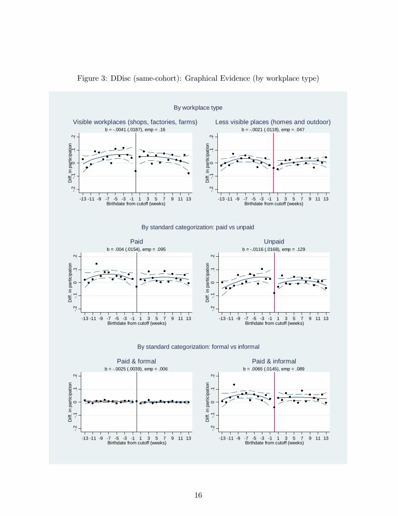
Figure 3: DDisc (same-cohort): Graphical Evidence (by workplace type)­.2

­.10

.1.2

Diff

. in 

parti

cipa

tion

­13 ­11 ­9 ­7 ­5 ­3 ­1 1 3 5 7 9 11 13Birthdate from cutoff (weeks)

b = ­.0041 (.0187), emp = .16Visible workplaces (shops, factories, farms)

­.2­.1

0.1

.2D

iff. i

n pa

rtici

patio

n

­13 ­11 ­9 ­7 ­5 ­3 ­1 1 3 5 7 9 11 13Birthdate from cutoff (weeks)

b = ­.0021 (.0118), emp = .047Less visible places (homes and outdoor)

By workplace type

­.2­.1

0.1

.2D

iff. i

n pa

rtici

patio

n

­13 ­11 ­9 ­7 ­5 ­3 ­1 1 3 5 7 9 11 13Birthdate from cutoff (weeks)

b = .004 (.0154), emp = .095Paid

­.2­.1

0.1

.2D

iff. i

n pa

rtici

patio

n

­13 ­11 ­9 ­7 ­5 ­3 ­1 1 3 5 7 9 11 13Birthdate from cutoff (weeks)

b = ­.0116 (.0168), emp = .129Unpaid

By standard categorization: paid vs unpaid

­.2­.1

0.1

.2D

iff. i

n pa

rtici

patio

n

­13 ­11 ­9 ­7 ­5 ­3 ­1 1 3 5 7 9 11 13Birthdate from cutoff (weeks)

b = ­.0025 (.0039), emp = .006Paid & formal

­.2­.1

0.1

.2D

iff. i

n pa

rtici

patio

n

­13 ­11 ­9 ­7 ­5 ­3 ­1 1 3 5 7 9 11 13Birthdate from cutoff (weeks)

b = .0065 (.0145), emp = .089Paid & informal

By standard categorization: formal vs informal

16

In all cases, graphical evidence shows that the e¤ect of the new ban was not e¤ective, not even

in visible activities where the law has more chances to be respected. The other categorizations

in Figure 3 are more standard: paid versus unpaid work and formal versus informal paid work.

Results corroborate previous �ndings about the absence of an employment e¤ect of the ban.

Table 2: Estimates based on Discontinuity in Treatment

Type Bandwidth RD(Sept. 1999)

DDisc(same cohort)

DDisc(same age)

Overall employment +/­ 3 ­0.0116 ­0.00628 0.0314(0.0387) (0.0220) (0.0201)

Overall employment +/­ 6 ­0.0345 0.000570 0.0298**(0.0307) (0.0151) (0.0140)

Visible employment +/­ 3 ­0.0215 ­0.00413 0.0118(0.0293) (0.0187) (0.0183)

Less visible employment +/­ 3 0.00981 ­0.00215 0.0196(0.0221) (0.0118) (0.0124)

Overall empl., urban +/­ 3 0.00878 ­0.00370 0.0290(0.0420) (0.0219) (0.0226)

Visible empl., urban +/­ 3 0.00136 ­0.00447 0.00522(0.0325) (0.0176) (0.0190)

Less visible empl., urban +/­ 3 0.00742 0.000762 0.0238*(0.0249) (0.0129) (0.0140)

RD: regression discontinuity, DDisc: difference­in­discontinuity. Estimations are based on a quadraticspline function of the running variable (sensitivity analysis is provided in the Appendix). Std errors inbrackets. *, **, *** indicate significance levels at 10%, 5%, 1%. Controls are child gender, ethnicity,household head's age, gender and years of schooling, region, rural, metropolitan area, assets, rate ofinspection, home ownership, household size. The R­squared is around 0.13 in RD and 0.15 in DDiscestimations with the 6­month bandwidth.

Estimations. The main estimation results are gathered in Table 2. We report the estimates

of � for the RD design (equation 1) carried out on 1999 data. We also present estimates of the

DDisc (equation 2) on pooled data, using either the same-cohort or the same-age comparison

groups for year 1998. Estimates are obtained with a quadratic spline speci�cation of the smooth

function �(�). The �rst row shows results with the 6-month bandwidth. Both RD and DDiscapproaches corroborate graphical evidence: we �nd no sign of a change in employment among

children subject to the ban. The second row gives similar result with the broader bandwidth.

Then we distinguish visible and less visible activities. The former type of child employment

yields a negative e¤ect with RD and same-cohort DDisc, twice larger than the e¤ect for less

17

detectable activities. In both cases, however, these e¤ects are not statistically signi�cant.

Finally, we replicate the estimations for urban children only (81:7% of the initial sample).

These are more likely to be employed in large �rms with higher chances of inspection. We

observe no major di¤erence in this case compared to results on the sample pooling rural and

urban households. In the Appendix, Table A.3 shows estimates for alternative speci�cations of

�(�) (linear, quadratic, cubic, linear spline), again with no particular di¤erence with the baselineestimates described above.

4.2 Power Calculations

A genuine concern pertains to the ability of our estimations to detect a signi�cant e¤ect of

the ban on child labor at the discontinuity. We carry out power calculation for RD and DDisc

designs (see Cattaneo et al., 2017, Schochet, 2008). In both case, the precision of estimated

treatment e¤ects is typically expressed in terms of minimum detectable e¤ect (MDE), i.e.

the smallest true treatment e¤ect that has a reasonable chance (usually a power of 80%) of

producing an estimated treatment e¤ect that is statistically signi�cant at the 5% level. We

will report MDE in percentage of the control group outcome (the employment rate of children

turning 14 just before the reform) as well as standardized MDE (MDE in percentage of the

standard deviation of the control group outcome).18

Results are presented in Figure 4. We focus on our favorite model, the DDisc design, and report

power levels for di¤erent bandwiths (6 or 12 months) and di¤erent de�nitions of the placebo

group (same-cohort or same-age children in 1998). In all cases, power increases with the size

of the e¤ect we want to detect (expressed in percentage of the control group mean outcome).

At the usual level of 80%, the 6-month bandwidth model using the same-cohort placebo can

detect an e¤ect no smaller than 27% of the unbanned children�s employment rate. In this case,

we obtain a standardized MDE of 14%, which is relatively small. The precision is best with

a large bandwidth and the same-age comparison group. In this case, we can detect a change

in child labor of at least 17% of the control group�s mean outcome (and a standardized MDE

of 10%). While these results apply to the overall employment e¤ect, we have replicated power

calculations for the other cases described above. In particular for the visible sector, in which we

would expect more compliance to the ban, results are slightly less precise due to the smaller size

18Formally, the MDE for a RD design is de�ned as:

MDE = 2:8

�(1�R2Y )�2Y

NP (1� P )(1�R2T )

�0:5with R2Y the coe¢ cient of determination of the statistical model, R

2T the correlation between treatment status

and the running variable, N the sample size and P the proportion of treated units.

18

of this group but nonetheless meaningful. As reported in Figure A.3 in the Appendix, we can

detect a change in child employment of at least 20%� 31% of the control group�s employment

rate.

Figure 4: Power (in percent of control group mean outcome) and MDE (at power = 80 percent)

for DDisc Treatment E¤ects

4.3 Heterogeneity and Additional Results

Heterogeneity in the Intensity of Labor Inspections. We check if there is heterogene-

ity in the e¤ect of the ban. It may possibly due to di¤erent degrees of enforcement across

regions concerned by various intensities of labor inspections. We simply replicate previous RD

and DDisc estimations while interacting the treatment variable with high and low intensity of

19

treatment de�ned as living in a state with above or below average rate of inspection by �rm

(Almeida and Carnero, 2009). Results are reported in Table 3. Interestingly, child labor seems

to decrease in high inspection states. This e¤ect is signi�cant with both the same-cohort and

the same-age DDisc designs. This result is con�rmed by the sensitivity analysis in Appendix

Table A.4. The e¤ect is not signi�cant with the RD when using the quadratic spline function

of the running variable. Yet, its magnitude is similar to DDisc estimates and, in Table A.4, we

see that all the other RD speci�cations con�rm the magnitude of the e¤ect while most of them

point to a signi�cant reduction.

Another interesting result is the decomposition by type of activity. We see that the new

minimum age tends to reduce child labor in high inspection states (i.e. where enforcement is

the highest) but only in child activities that are most visible (i.e. where compliance is expected

to be the highest). This intuitive result is very stable across models and speci�cations (as can

be seen in Appendix Table A.4). It leads to a magnitude between 5:5 and 7 percentage points

depending on the estimation, i.e. a reduction between a third and 40% compared to the visible

employment rate of the control group (17%).

Table 3: Estimates by Inspection Intensity

RD(Sept. 1999)

DDisc(same cohort)

DDisc(same age)

Overall employment Low inspection states 0.00433 0.0176 0.0621***(0.0395) (0.0251) (0.0232)

High inspection states ­0.0677 ­0.0802** ­0.0675*(0.0452) (0.0339) (0.0354)

Visible employment Low inspection states ­0.00888 0.0173 0.0328(0.0300) (0.0218) (0.0209)

High inspection states ­0.0629* ­0.0711** ­0.0562*(0.0367) (0.0297) (0.0317)

Less visible employment Low inspection states 0.0132 0.000284 0.0294**(0.0228) (0.0139) (0.0144)

High inspection states ­0.00482 ­0.00912 ­0.0113(0.0250) (0.0184) (0.0192)

Type

Coefficients of treatment effect interacted with low/high inspection rate state. RD: regression discontinuity, DDisc:difference­in­discontinuity, both using 6­month bandwidth. Estimations are based on a quadratic spline function ofthe running variable (sensitivity analysis is provided in the Appendix). Std errors in brackets. *, **, *** indicatesignificance levels at 10%, 5%, 1%. Controls are child gender, ethnicity, household head's age, gender and years ofschooling, region, rural, metropolitan area, assets, rate of inspection, home ownership, household size.

Our measure of enforcement is based on a state average of local rates of inspection per �rm. Since

this is a very broad measure, we have attempted to disaggregate the information a bit more.

20

In the left panel of Appendix Table A.5, we replicate estimations using the inspection rates

averaged at state � rural/urban level to obtain more variation. This is especially important asthe intensity of inspection tends to be larger in urban areas. In the right panel of the table,

we report estimates focusing on urban households. In both cases, results are very much in line

with previous �ndings and point to a signi�cant e¤ect in visible activities when the chances of

inspections are high.

Table 4: Estimates: Additional Heterogeneity

Type All sectorsVisible activities,low inspection

Visible activities,high inspection

Less visibleactivities

Boys (main selection) 0.0116 0.0504 ­0.0942** ­0.00199(0.0319) (0.0352) (0.0440) (0.0167)

Girls (main selection) ­0.0216 ­0.00910 ­0.0334 ­0.00681(0.0263) (0.0244) (0.0318) (0.0152)

Siblings (unbanned, aged 14­16) ­0.0125 0.00533 ­0.0152 ­0.0110(0.0621) (0.0759) (0.101) (0.0252)

Difference­in­discontinuity with 6­month bandwidth and a quadratic spline function of the running variable (sensitivity checksshow similar results with alternative specifications ­ these additional results are available from the authors). Std errors inbrackets. *, **, *** indicate significance levels at 10%, 5%, 1%. Controls are child gender, ethnicity, household head's age,gender and years of schooling, region, rural, metropolitan area, assets, rate of inspection, home ownership, household size.

Additional Results. To re�ne the picture, a set of heterogeneous e¤ects is reported in Table

4 using the same-cohort DDisc with the 6-month bandwidth (alternative models lead to similar

results as what follows). We see that the main e¤ect of the ban, i.e. a decline in visible

activities in places with high risk of inspection, is only signi�cant among boys. A larger and

more precisely estimated response from boys was expected given their much higher rate of

economic activity (27%) compared to girls (14%) in 1999, especially in visible activities (23%

versus 8:5%). The magnitude of the e¤ect (9:4 points) relative to the 1999 employment rate

of boys in visible activities (25%) yields a 38% reduction, in line with the overall e¤ect found

before. Even if not statistically signi�cant, the e¤ect for girls is similar in size (3:3 point drop

in visible employment rate relative to a 8:8% employment rate in the control group, hence a

37:5% decline).

The rest of Table 4 checks potential compensatory e¤ects by other household members (see

also Bharadwaj et al., 2013). We have already commented on the fact that these substitution

21

e¤ects within families are not visible in our bandwidth when using the same-age placebo as a

counterfactual employment-age pattern. This is con�rmed by additional estimations using our

selected children�s birthdate as forcing variable and the average employment outcome of their

older siblings (aged 14-16) as outcome. Finally, it is possible that the law triggers responses

regarding other outcomes. Among unreported results, we have checked the potential e¤ect of

the new law on school enrollment of children around age 14. We found no signi�cant e¤ect.

We also found no particular changes in wage rates.

5 Conclusion

This paper provides evidence on the potential e¤ect of a child labor ban exerted by a legal age

condition. We exploit the change in the age limit in Brazil, raised from 14 to 16 years old in

December 1998. We exploit heterogeneous eligibility among children who turned 14 around the

reform date. Local identi�cation in RD and DDisc designs escapes from the usual di¢ culty

of age trend methods like DD with broad comparison groups on each side of the cuto¤. We

nonetheless �nd enough power to detect reasonable e¤ects. We �nd no e¤ect of the ban on

child employment overall but a signi�cant and quite substantial reducing e¤ect on children in

visible activities in regions where enforcement is potentially high.

Our results tend to con�rm previous evidence on the relatively weak e¤ectiveness of minimum

age regulation (Edmonds, 2014). Yet we have also established that there is substantial het-

erogeneity depending on the degree of enforcement. Children in rural areas or in activities

that are not easily subject to enforcement measures will probably not be a¤ected by minimum

age policies. Other children in visible activities, for instance paid children working with or

without a labor card in large �rms, may be compelled to withdraw from this type of job by

their employers. Yet the e¤ect is diluted and we could only provide suggestive evidence using

heterogeneity across broad job types (more or less visible �rms) and enforcement degrees (in-

spection intensity). Further work should attempt to collect more precise data on the degree of

potential enforcement, possibly around future change in minimum age laws in other countries.

More detailed variation could also allow detecting whether reallocation of children occurs across

speci�c sectors. Finally, better data could say something about the potential impact of a ban

on the worst forms of child labor. The literature points to the fact that legal bans may establish

new societal norms and provide tools for the legal system to go after �rms in case of forced

labor (Swinnerton and Rogers, 2008). Legal measures against hazardous did not concern the

14-year old discontinuity exploited in our study, so we could not address this question. More

generally, given the small share of children concerned by this type of work, very detailed data

should be collected to identify potential shifts of children out of detrimental sectors.

22

References

[1] Almeida, R. and P. Carneiro (2009): "Enforcement of labor regulation and �rm size,"

Journal of Comparative Economics, 37(1), 28-46

[2] Almeida, R. and P. Carneiro (2012): "Enforcement of Labor Regulation and Informality,"

American Economic Journal: Applied Economics, 4(3), 64-89

[3] Baland, J.-M. and Robinson, J. A. (2000): "Is child labor ine¢ cient?", Journal of Political

Economy, 108 (4), 663�679

[4] Bargain, O. and P. Kwenda (2014): "The Informal Sector Wage Gap: New Evidence Using

Quantile Estimations on Panel Data", Economic Development and Cultural Change,

63(1), 117�153

[5] Basu, K., and Van, P.H. (1998): "The economics of child labor." American Economic

Review, 412-427

[6] Basu, K. (2005): "Child labor and the law: Notes on possible pathologies", Economic

Letters 87:2, 169�174

[7] Bertrand, M., E. Du�o and S. Mullainathan (2004): "How Much Should We Trust

Di¤erences-In-Di¤erences Estimates?", Quarterly Journal of Economics, 119 (1), 249-

275

[8] Bharadwaj, P., Lakdawala, L. K., and Li, N. (2013): "Perverse Consequences of Well-

Intentioned Regulation: Evidence from India�s Child Labor Ban", NBER Working

Paper No. 19602

[9] Bon�m de Almeida, R. and A.L. Kassouf (2016): "The e¤ect of labor inspections on

reducing child labor in Brazil", UCW working paper

[10] Boockmann, B. (2010): "The E¤ect of ILO Minimum Age Conventions on Child La-

bor�and School Attendance: Evidence From Aggregate and Individual-Level Data",

World Development, 38(5), 679-692

[11] Cardoso, F. H. (1997): "Trabalho infantil no Brasil: questões e politicas", in: Conferência

de Oslo

[12] Cattaneo, M. D., Titiunik, R., and Vazquez-Bare, G. (2017) : "Power calculations for

regression discontinuity designs", Working Paper, University of Michigan

[13] Coslovsky, S.V. (2014): "Flying under the radar? The state and the enforcement of labour

laws in Brazil", Oxford Development Studies, 42(2), 190�216

[14] Dessy, S. E. (2000): "A defense of compulsory measures against child labor", Journal of

Development Economics, 62 (1), 261�27

23

[15] Dessy, S. E. and S. Pallage (2005): "A Theory of the worst form of child labour", Economic

Journal, 115, 68�87

[16] Del Vecchio, P. (2005): "Child Labor in Brazil, The Government Commitment", Economic

Perspectives, U.S. Department of State, may 2005, volume 10, no.2

[17] Dong, Y. (2015): "Regression Discontinuity Applications with Rounding Errors in the

Running Variable.", Journal of Applied Econometrics 30 (3):422-446.

[18] Edmonds, E.V. (2008): "Child Labour", in Schultz, T.P. and Strauss, J. Handbook of

Development Economics, Vol. 4. Elsevier, Amsterdam, North Holland

[19] Edmonds, E.V. (2014): "Does minimum age of employment regulation reduce child la-

bor?", IZA World of Labour, 73

[20] Edmonds, E.V. and M. Shrestha (2012): "The Impact of Minimum Age of Employment

Regulation on Child Labor and Schooling", IZA Journal of Labor Policy 1(14), 1-28

[21] Ferro, A.R. and A.L. Kassouf (2005): "Efeitos do aumento da idade minima legal no

trabalho dos brasileiros de 14 e 15 anos", Revista de Economia e Sociologia Rural,

43(2), 307�329

[22] Fortin, B., Lacroix, G., Drolet, S. (2004): "Welfare bene�ts and the duration of welfare

spells: evidence from a natural experiment in Canada". Journal of Public Economics

88, 1495�1520

[23] Grembi, V., T. Nannicini and U. Troiano (2016): "Do Fiscal Rules Matter?" (a Di¤erence-

in-Discontinuities Design), forthcoming in American Economic Journal: Applied Eco-

nomics

[24] Henley, A., G.R. Arabsheibani and F. Carneiro (2009): "On De�ning and Measuring the

Informal Sector", World Development, 37, 5, 992-1003

[25] Imbens, G. and T. Lemieux (2008): �Regression Discontinuity Designs: A Guide to Prac-

tice�, Journal of Econometrics, 142 (2), 615�635

[26] Lee, D.S. and Card, D. (2008): "Regression discontinuity inference with speci�cation er-

ror", Journal of Econometrics, 142(2), 655-674

[27] Lee, D. S. and T. Lemieux (2010): "Regression discontinuity designs in economics", Journal

of Economic Literature 48 (2), 281�355

[28] Lemieux, T. and K. Milligan (2008): "Incentive e¤ects of social assistance: a regression

discontinuity approach", Journal of Econometrics, 142(2), 807�828

[29] Manacorda, M. (2006): "Child Labour and the Labour Supply of Other Household Mem-

bers: Evidence from 1920 America", American Economic Review, 96, 5, 1788-1801

24

[30] Margo, R., and A. Finegan (1996): "Compulsory schooling legislation and school atten-

dance in turn of the century America: A natural experiment approach", Economic

Letters 53, 103�110

[31] McCrary, J. (2008): "Manipulation of the running variable in the regression discontinuity

design: a density test", Journal of Econometrics, 142(2), 698-714

[32] Moehling, C. (1999): "State child labor laws and the decline of child labor", Explorations

in Economic History 36, 72�106

[33] Paes-Sousa, R., L.M Santos and E.S. Miazaki (2011): "E¤ects of a conditional cash transfer

programme on child nutrition in Brazil", Bulletin of the World Health Organization,

89(7), 496-503

[34] Piza, C. and A. Portela Souza (2016): "The Causal Impacts of Child Labor Law

in Brazil: Some Preliminary Findings", World Bank Economic Review, doi:

10.1093/wber/lhw024

[35] Ranjan, P. (1999): "An economic analysis of child labor", Economics Letters, 64 (1),

99�105

[36] Rosati, F.C, M. Manacorda, I. Kovrova, N. Koseleci, S. Lyon (2011): "Understanding

the Brazilian success in reducing child labour: empirical evidence and policy lessons",

Understanding Children�s Work report, ILO

[37] Schochet, P. Z. (2008): "Technical Methods Report: Statistical Power for Regression

Discontinuity Designs in Education Evaluations", NCEE 2008-4026, Washington, DC:

National Center for Education Evaluation and Regional Assistance.

[38] Silva, P., D. Pessoa and M. Lila (2002): "Análise estatística de dados da PNAD: in-

corporando a estrutura do plano amostral" (Statistical analysis of data from PNAD:

incorporating the sample design), Ciência e Saúde Coletiva, 7(4), 659-670

[39] Somers, M., Zhu, P., Jacob, R. and Bloom, H. (2013): "The validity and precision of the

comparative interrupted time series design and the di¤erence-in-di¤erence design in

educational evaluation", MDRC working paper in research methodology, NY

[40] Swinnerton, K., and C. Rogers (2008): "A theory of exploitative child labor", Oxford

Economic Papers 60, 20�41

[41] UNESCO (2017): "The e¤ect of varying population estimates on the calculation of en-

rolment rates and out-of-school rates ", UNESCO Institute for Statistics, information

paper 36

25

A Appendix

A.1 Alternative Bandwidth

Table A.1: Treatment and Control Groups with the +/- 6 Months Window

Cohort definition age inSept. 98

subject toold ban

subject tonew ban

allowed towork

Cohort definition age inSept. 98

subject toold ban

subject tonew ban

allowed towork

Turned 14 between Dec 15 1998and Mars 15 1999 13 yes ­ no

Turned 14 between Dec 15 1997and Mars 15 1998 14 no ­ yes

Turned 14 between Mars 151999 and June 15 1999 13 yes ­ no

Turned 14 between Mars 151998 and June 15 1998 14 no ­ yes

Turned 14 between June 15 1998and Sept 15 1998 14 no ­ yes

Turned 14 between June 15 1997and Sept 15 1997 15 no ­ yes

Turned 14 between Sept 15 1998and Dec 15 1998 13 yes ­ no

Turned 14 between Sept 15 1997and Dec 15 1997 14 no ­ yes

Cohort definition age inSept. 99

subject toold ban

subject tonew ban

allowed towork

Cohort definition age inSept. 99

subject toold ban

subject tonew ban

allowed towork

Turned 14 between Dec 15 1998and Mars 15 1999 14 ­ yes no

Turned 14 between Dec 15 1998and Mars 15 1999 14 ­ yes no

Turned 14 between Mars 151999 and June 15 1999 14 ­ yes no

Turned 14 between Mars 151999 and June 15 1999 14 ­ yes no

Turned 14 between June 15 1998and Sept 15 1998 15 ­ no yes

Turned 14 between June 15 1998and Sept 15 1998 15 ­ no yes

Turned 14 between Sept 15 1998and Dec 15 1998 14 ­ no yes

Turned 14 between Sept 15 1998and Dec 15 1998 14 ­ no yes

Same cohort, different age Same age, consecutive cohorts

Treatment "banned from work due to minimal age condition" indicated in grey. It isdue to old ban for only 3/4 of the 1998 observations and to new ban for the first half­cohort in 1999.

Treatment "banned from work due to minimal age condition" indicated in grey. It isdue to the new ban for the first half­cohort in 1999.

PNAD 1998

PNAD 1999

PNAD 1998

PNAD 1999

26

A.2 Comparing Sub-Cohorts around the Cuto¤

Table A.2 shows descriptive statistics for our 1999 selection with either the 6-month or 12-month

bandwiths around the cuto¤. The main observation is that characteristics of the subcohorts on

either side of the birthdate threshold are rarely statistically di¤erent. Whatever the bandwidth,

a F-test cannot reject the null that the two sub-cohorts have the same characteristics. Yet, as

expected, the broader bandwith shows more di¤erences between the two subgroups than the

narrow bandwith does.

Table A.2: Descriptive Statistics around the Cuto¤ (year 1999)

birth <midDec

birth >mid Dec

birth <midDec

birth >mid Dec

Region Norte 0.09 0.07 ­0.02 ** 0.09 0.07 ­0.02 ***Region Nordeste 0.32 0.35 0.03 * 0.33 0.36 0.03 **Region Sudeste 0.33 0.32 ­0.01 0.33 0.32 ­0.01Region Sul 0.16 0.17 0.01 0.16 0.16 0.00Rural 0.21 0.21 0.00 0.21 0.21 0.00Metropolitan area 0.37 0.39 0.02 0.36 0.38 0.02Ethnicity (branca) 0.49 0.52 0.03 0.48 0.48 0.00Ethnicity (parda) 0.46 0.44 ­0.02 0.46 0.48 0.02Head: education 5.30 5.41 0.11 5.16 5.31 0.15Head: mother 0.22 0.20 ­0.02 0.22 0.20 ­0.02 *Head: age 43.69 43.59 ­0.1 43.70 43.54 ­0.16Assets 5.01 5.06 0.05 4.96 5.02 0.06Inspection intensity 4.53 4.43 ­0.1 4.42 4.34 ­0.08Home owner 0.75 0.73 ­0.02 0.74 0.73 ­0.01Household size 5.45 5.37 ­0.08 5.44 5.35 ­0.09 **, **, *** indicates significant difference in mean characteristics at the 10%, 5%, 1% significance levels respectively.

6­month bandwidth

Diff.

12­month bandwidth

Diff.

27

A.3 Errors and Manipulation of Birthdate

Birth registration is compulsory in Brazil. Without birth certi�cates children cannot be vacci-

nated or enrolled in school, and unregistered adult cannot obtain a worker�s card. This should

limit measurement error. It also establishes that �rms are in principle aware of the precise

age of their workforce. Yet, while the vast majority of children have a birth certi�cate, due

to increased access to birth registration (UNICEF, 2017), a non-negligible fraction of children

had no birth certi�cate in rural areas.19 In the text, we provide sensitivity checks whereby we

exclude the rural population. Here, we also verify that the birthdate density in our selection

shows no discontinuous jump just before the reform date, which would indicate age manipula-

tion in the PNAD data (McCrary, 2008). If we misclassify children due to misreporting of their

exact age, we should observe a discontinuity in birthdate density around the cuto¤. Figure A.1

shows that in September 1999, with both 6-month and 12-month bandwidths (upper and lower

left panels respectively), we �nd no signi�cant di¤erence in birthdate density. Formal tests

cannot reject the null hypothesis of equal density. Note that the slight decrease on the left of

the cuto¤ is actually opposite to what we would expect in case of misdeclaration to avoid the

new ban (i.e. more children to the left of the cuto¤). For a comparison, we also provide similar

graphs for 1998 (right panel), using the same-age (previous cohort) children. The distribution

of birthdates is relatively uniform across time around mid-December, as was the case for 1999.

19This would concern around 20% of children in the late 1990s according to IBGE, especially among indigenous

populations. According to Paes-Souza et al. (2011), the lack of certi�cate is an indicator of extreme poverty

and of residence in an isolated area.

28

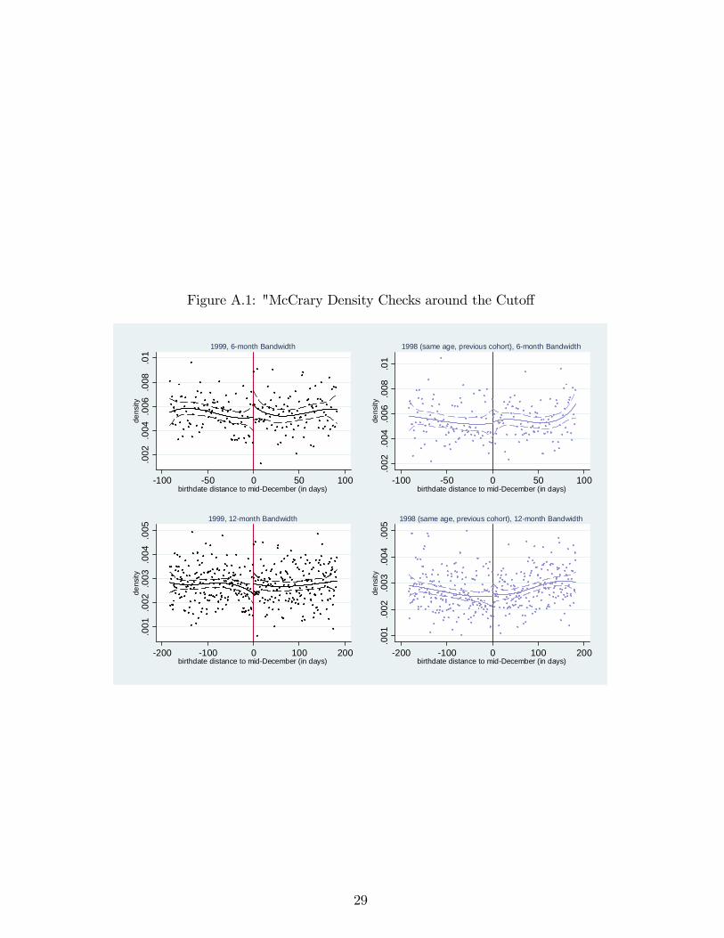
Figure A.1: "McCrary Density Checks around the Cuto¤

.002

.004

.006

.008

.01

dens

ity

­100 ­50 0 50 100birthdate distance to mid­December (in days)

1999, 6­month Bandwidth

.002

.004

.006

.008

.01

dens

ity

­100 ­50 0 50 100birthdate distance to mid­December (in days)

1998 (same age, previous cohort), 6­month Bandwidth

.001

.002

.003

.004

.005

dens

ity

­200 ­100 0 100 200birthdate distance to mid­December (in days)

1999, 12­month Bandwidth

.001

.002

.003

.004

.005

dens

ity

­200 ­100 0 100 200birthdate distance to mid­December (in days)

1998 (same age, previous cohort), 12­month Bandwidth

29

A.4 Sensitivity Analysis and Additional Results

Figure A.2: RD and DDisc (same-age): Graphical Evidence (Total Employment, 6-months

Bandwidth)

1314

15Ag

e (c

ross

es)

0.1

.2.3

.4pa

rtici

patio

n (d

ots)

­13 ­11 ­9 ­7 ­5 ­3 ­1 1 3 5 7 9 11 13Birthdate from cutoff (weeks)

RD 1998: b = ­.1158 (.0516), emp = .219

1314

15Ag

e (c

ross

es)

0.1

.2.3

.4pa

rtici

patio

n (d

ots)

­13 ­11 ­9 ­7 ­5 ­3 ­1 1 3 5 7 9 11 13Birthdate from cutoff (weeks)

RD 1999: b = ­.0116 (.0387), emp = .207

0.1

.2.3

.4pa

rtici

patio

n (d

ots)

­13 ­11 ­9 ­7 ­5 ­3 ­1 1 3 5 7 9 11 13Birthdate from cutoff (weeks)

1999

1998

RD: Both Years

­.2­.1

0.1

.2D

iffer

ence

 in p

artic

ipat

ion 

(dot

s)

­13 ­11 ­9 ­7 ­5 ­3 ­1 1 3 5 7 9 11 13Birthdate from cutoff (weeks)

Diff­in­Discontinuity: b = .0314 (.0201)

Trend lines obtained using a quadratic spline specification. Dashed lines represent the 95% CI. Crosses (in upper graphs) indicate the age

Cohorts born +/­ 3 months around mid­Dec 1984 (1999) and mid­Dec 1983 (1998)All children,  % Economically Active

30

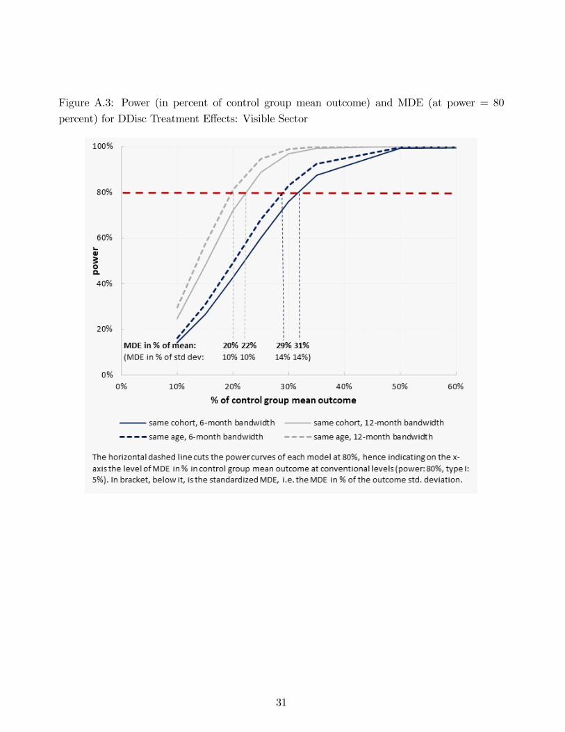
Figure A.3: Power (in percent of control group mean outcome) and MDE (at power = 80

percent) for DDisc Treatment E¤ects: Visible Sector

31

Table A.3: Estimates based on Discontinuity in Treatment: Sensitivity Analysis�

Type Bandwidth linear quadratic cubiclinearspline linear quadratic cubic

linearspline linear quadratic cubic

linearspline

Overall employment 6 months ­0.0119 ­0.0120 ­0.00632 ­0.0119 ­0.00620 ­0.00623 ­0.00630 ­0.00625 0.0315 0.0315 0.0312 0.0316(0.0289) (0.0290) (0.0392) (0.0288) (0.0220) (0.0220) (0.0220) (0.0220) (0.0202) (0.0202) (0.0201) (0.0202)

Overall employment 12 months 0.0194 0.0195 ­0.0270 0.0195 0.000575 0.000538 0.000566 0.000545 0.0300** 0.0300** 0.0299** 0.0300**(0.0214) (0.0212) (0.0275) (0.0211) (0.0151) (0.0151) (0.0151) (0.0151) (0.0141) (0.0141) (0.0140) (0.0141)

Visible employment 6 months ­0.0221 ­0.0221 ­0.0198 ­0.0221 ­0.00412 ­0.00414 ­0.00414 ­0.00416 0.0120 0.0120 0.0118 0.0120(0.0226) (0.0228) (0.0295) (0.0227) (0.0187) (0.0187) (0.0187) (0.0187) (0.0184) (0.0184) (0.0183) (0.0184)

Less visible employment 6 months 0.0101 0.0101 0.0135 0.0102 ­0.00208 ­0.00209 ­0.00216 ­0.00209 0.0196 0.0196 0.0195 0.0196(0.0159) (0.0159) (0.0207) (0.0158) (0.0118) (0.0118) (0.0118) (0.0118) (0.0124) (0.0124) (0.0124) (0.0124)

Overall empl., urban 6 months ­0.00781 ­0.00735 0.0102 ­0.00699 ­0.00353 ­0.00370 ­0.00370 ­0.00373 0.0284 0.0284 0.0285 0.0285(0.0339) (0.0333) (0.0462) (0.0323) (0.0220) (0.0220) (0.0220) (0.0220) (0.0226) (0.0226) (0.0226) (0.0226)

Visible empl., urban 6 months ­0.0151 ­0.0149 ­0.000439 ­0.0146 ­0.00442 ­0.00452 ­0.00445 ­0.00455 0.00491 0.00495 0.00495 0.00500(0.0268) (0.0265) (0.0362) (0.0259) (0.0177) (0.0176) (0.0176) (0.0176) (0.0190) (0.0189) (0.0190) (0.0189)

Less visible empl., urban 6 months 0.00726 0.00754 0.0107 0.00760 0.000895 0.000819 0.000753 0.000820 0.0235* 0.0235* 0.0235* 0.0235*(0.0185) (0.0183) (0.0234) (0.0182) (0.0129) (0.0129) (0.0129) (0.0129) (0.0140) (0.0140) (0.0140) (0.0140)

RD (Sept. 1999) DDisc (same cohort) DDisc (same age)

RD: regression discontinuity, DDisc: difference­in­discontinuity. Estimations are based on alternative smooth functions of the running variable (linear, quadratic, cubic, linearspline). Std errors in brackets. *, **, *** indicate significance levels at 10%, 5%, 1%. Controls are child gender, ethnicity, household head's age, gender and years of schooling,region, rural, metropolitan area, assets, rate of inspection, home ownership, household size. The R­squared is around 0.13 in RD estimations and 0.15 in DDisc estimations withthe 6­month bandwidth.

32

Table A.4: Estimates by Inspection Intensity: Sensitivity Analysis

Type linear quadratic cubiclinearspline linear quadratic cubic

linearspline linear quadratic cubic

linearspline

Overall empl. Low inspect. 0.00483 0.00479 0.00965 0.00493 0.0176 0.0176 0.0176 0.0176 0.0616*** 0.0616*** 0.0616*** 0.0617***(0.0302) (0.0303) (0.0398) (0.0300) (0.0251) (0.0251) (0.0251) (0.0251) (0.0233) (0.0233) (0.0232) (0.0233)

High inspect. ­0.0661* ­0.0660* ­0.0610 ­0.0662* ­0.0800** ­0.0801** ­0.0803** ­0.0801** ­0.0652* ­0.0652* ­0.0663* ­0.0653*(0.0361) (0.0362) (0.0462) (0.0359) (0.0338) (0.0338) (0.0339) (0.0338) (0.0355) (0.0355) (0.0355) (0.0355)

Visible empl. Low inspect. ­0.00933 ­0.00943 ­0.00735 ­0.00934 0.0173 0.0173 0.0173 0.0173 0.0326 0.0327 0.0326 0.0327(0.0237) (0.0239) (0.0301) (0.0238) (0.0218) (0.0218) (0.0218) (0.0218) (0.0209) (0.0209) (0.0209) (0.0209)

High inspect. ­0.0628** ­0.0627** ­0.0606 ­0.0628** ­0.0711** ­0.0712** ­0.0712** ­0.0712** ­0.0551* ­0.0551* ­0.0559* ­0.0552*(0.0309) (0.0310) (0.0372) (0.0309) (0.0297) (0.0297) (0.0297) (0.0297) (0.0316) (0.0316) (0.0316) (0.0316)

Less visible empl. Low inspect. 0.0142 0.0142 0.0170 0.0143 0.000322 0.000322 0.000272 0.000319 0.0290** 0.0289** 0.0289** 0.0290**(0.0168) (0.0167) (0.0214) (0.0167) (0.0139) (0.0139) (0.0139) (0.0139) (0.0144) (0.0144) (0.0144) (0.0144)

High inspect. ­0.00325 ­0.00330 ­0.000452 ­0.00342 ­0.00896 ­0.00897 ­0.00913 ­0.00897 ­0.0101 ­0.0101 ­0.0103 ­0.0101(0.0202) (0.0202) (0.0240) (0.0202) (0.0184) (0.0184) (0.0184) (0.0184) (0.0192) (0.0192) (0.0192) (0.0192)

RD (Sept. 1999) DDisc (same cohort) DDisc (same age)

Coefficients of treatment effect interacted with low/high inspection rate state. RD: regression discontinuity, DDisc: difference­in­discontinuity, both using 6­month bandwidth. Estimations are based onalternative smooth functions of the running variable (linear, quadratic, cubic, linear spline). Std errors in brackets. *, **, *** indicate significance levels at 10%, 5%, 1%. Controls are child gender, ethnicity,household head's age, gender and years of schooling, region, rural, metropolitan area, assets, rate of inspection, home ownership, household size.

Table A.5: Estimates by Inspection Intensity: More Geographical Variation

RD(Sept. 1999)

DDisc(same cohort)

DDisc(same age)

RD(Sept.1999)

DDisc(same

cohort)

DDisc(same age)

Overall employment Low inspection states 0.00972 0.0113 0.0766*** 0.0275 0.0183 0.0577**(0.0405) (0.0279) (0.0250) (0.0420) (0.0243) (0.0265)

High inspection states ­0.0413 ­0.0326 ­0.0366 ­0.0521 ­0.0626* ­0.0516(0.0419) (0.0257) (0.0275) (0.0500) (0.0335) (0.0337)

Visible employment Low inspection states 0.00318 0.0200 0.0500** ­0.00888 0.0151 0.0221(0.0308) (0.0250) (0.0227) (0.0329) (0.0201) (0.0227)

High inspection states ­0.0569** ­0.0406* ­0.0458* ­0.0555* ­0.0578** ­0.0416(0.0267) (0.0219) (0.0246) (0.0310) (0.0273) (0.0276)

Less visible employment Low inspection states 0.00655 ­0.00866 0.0266 0.0129 0.00317 0.0356**(0.0246) (0.0156) (0.0164) (0.0254) (0.0155) (0.0162)

High inspection states 0.0136 0.00800 0.00923 ­0.0116 ­0.00480 ­0.00995(0.0217) (0.0139) (0.0145) (0.0284) (0.0192) (0.0202)

Type

More disaggregated inspection rate Urban sample

Coefficients of treatment effect interacted with low/high inspection rate state. RD: regression discontinuity, DDisc: difference­in­discontinuity, both using 6­monthbandwidth. Estimations are based on a quadratic spline function of the running variable (sensitivity analysis is provided in the Appendix). Std errors in brackets. *,**, *** indicate significance levels at 10%, 5%, 1%. Controls are child gender, ethnicity, household head's age, gender and years of schooling, region, rural,metropolitan area, assets, rate of inspection, home ownership, household size. More disaggregated inspection intensity is the rate at state x rural/urban level.

33