minimum-variance multitaper spectral estimation on …€¦ · · 2010-10-28minimum-variance...
TRANSCRIPT

The Journal of Fourier Analysis and Applications
Volume 13, Issue 6, 2007
Minimum-Variance MultitaperSpectral Estimation on the
Sphere
Mark A. Wieczorek and Frederik J. Simons
Communicated by Matthias Holschneider
ABSTRACT. We develop a method to estimate the power spectrum of a stochastic process onthe sphere from data of limited geographical coverage. Our approach can be interpreted eitheras estimating the global power spectrum of a stationary process when only a portion of the dataare available for analysis, or estimating the power spectrum from local data under the assumptionthat the data are locally stationary in a specified region. Restricting a global function to a spatialsubdomain — whether by necessity or by design — is a windowing operation, and an equation likea convolution in the spectral domain relates the expected value of the windowed power spectrum tothe underlying global power spectrum and the known power spectrum of the localization window.The best windows for the purpose of localized spectral analysis have their energy concentratedin the region of interest while possessing the smallest effective bandwidth as possible. Solvingan optimization problem in the sense of Slepian (1960) yields a family of orthogonal windows ofdiminishing spatiospectral localization, the best concentrated of which we propose to use to forma weighted multitaper spectrum estimate in the sense of Thomson (1982). Such an estimate isboth more representative of the target region and reduces the estimation variance when comparedto estimates formed by any single bandlimited window. We describe how the weights applied tothe individual spectral estimates in forming the multitaper estimate can be chosen such that thevariance of the estimate is minimized.
1. Introduction
Spectral analysis is an indispensable tool in many branches of the physical and mathematicalsciences, with common applications ranging from one-dimensional time series to two-dimensional image analysis. For many purposes it is sufficient to employ a Cartesiangeometry, and for this case a plethora of sophisticated techniques have been developed,such as parametric, maximum-entropy, and multitaper spectral analysis (see [18] for a
Math Subject Classifications. 33C55, 34L05, 42B35, 42C10, 62M15.Keywords and Phrases. Spherical harmonics, multitaper spectral analysis.
© 2007 Birkhäuser Boston. All rights reservedISSN 1069-5869 DOI: 10.1007/s00041-006-6904-1

666 Mark A. Wieczorek and Frederik J. Simons
comprehensive review). However, for certain problems, especially in geophysics, it isnecessary to obtain spectral estimates from data that are localized to specific regions on thesurface of a sphere. While subsets of these data could be mapped to a two-dimensional plane,enabling the use of Cartesian methods, this procedure is bound to introduce some error intothe obtained spectral estimates. As the size of the region approaches a significant fractionof the surface area of the sphere, these would naturally become increasingly unreliable.
Spectral analysis on the sphere is an important tool in several scientific disciplines,and two examples suffice to illustrate the range of problems that are often encountered.First, in geophysics and geodesy it is common to represent the gravity field and topographyof the terrestrial planets as spherical harmonic expansions and to use their cross-spectralproperties to investigate the interior structure of the body [29]. However, since the relation-ship between the gravity and topography coefficients depends upon the geologic history ofthe geographic area of interest, it is often necessary to consider only a localized subset ofthese data. A second example is in the field of cosmology where the power spectrum ofthe cosmic microwave background radiation is used to place important constraints on thestructure and constitution of the universe [25]. In contrast to many geophysical problems,the measured temperature fluctuations are often assumed to be derived from a globallystationary process. Nevertheless, when estimating the power spectrum from satellite andterrestrial-based measurements, it is necessary to mask out regions that are contaminatedby emissions emanating from the plane of our own galaxy [9].
On the sphere one is thus concerned generally with estimating the power spectrumof a certain process from data confined to a restricted region. As illustrated by the aboveexamples, this can be interpreted in one of two ways. In one case, the function is assumed tobe stationary, and an estimate of the global power spectrum is desired based on a localizedsubset of data. In the second case, the data are known to be nonstationary, and an estimateof a “localized” power spectrum is sought by assuming local stationarity of the data withinthe specified region.
The restriction of data to a specified region is equivalent to multiplying a globallydefined function by a localization window or “data taper,” and the objective is to relatethe power spectrum of this localized field to the global one. This has been investigatedby using single binary masks [10], as well as families of orthogonal isotropic windowswith the purpose of obtaining a “multitaper” estimate [31]. The use of multiple localizationwindows, as originally pioneered in the Cartesian domain by Thomson [26], possesses manyadvantages over that of a single window, in particular, smaller variances of the resultingspectral estimates and more uniform coverage of the localization region. Here, we extendour previous approach [31] of using zonal tapers (i.e., those with azimuthal symmetryabout a polar axis) to the general case that includes nonzonal tapers [21]. The inclusionof nonzonal data tapers greatly increases the number of individual spectral estimates thatmake up the multitaper estimate, and this leads to a significant reduction in the variance ofthis estimate. We demonstrate how the weights of the individual estimates can be chosento minimize the multitaper estimation variance.
In this article, we first describe the theory of estimating the global power spectrumof a stochastic stationary process through the use of localization windows. This includesquantifying the relationship between the global and localized power spectra, the designof windows that are optimal for this purpose, and the formation of a minimum-variancemultitaper spectral estimate. The majority of the theoretical development relating to theseproblems is contained in four appendices. Following this, we describe the statistical prop-erties of the multitaper estimates (such as their bias and variance) heuristically when thedata are governed by a stochastic process with either a “white” or “red” power spectrum.

Minimum-Variance Multitaper Spectral Estimation on the Sphere 667
Next, we give an example of estimating the power spectrum from a single realization of astochastic process. Finally, we conclude by emphasizing avenues of future research.
2. Theory
2.1 Localized Spectral Estimation
Any real square-integrable function on the unit sphere can be expressed by a linear combi-nation of orthogonal functions as
f (�) =∞∑l=0
l∑m=−l
flmYlm(�) , (2.1)
where Ylm is a real spherical harmonic of degree l and order m, flm is the correspondingexpansion coefficient, and � = (θ, φ) represents position on the sphere in terms of colat-itude, θ , and longitude, φ. The real spherical harmonics are defined in terms of a productof a Legendre function in colatitude and either a sine or cosine function in longitude,
Ylm(�) ={
P̄lm(cos θ) cos mφ if m ≥ 0P̄l|m|(cos θ) sin |m|φ if m < 0 ,
(2.2)
and the normalized Legendre functions used in this investigation are given by
P̄lm(µ) = √(2 − δ0m)(2l + 1)
√(l − m)!(l + m)! Plm(µ) , (2.3)
where δij is the Kronecker delta function and Plm is the standard associated Legendre func-tion,
Plm(µ) = 1
2l l!(
1 − µ2)m/2
(d
dµ
)l+m (µ2 − 1
)l
. (2.4)
With the above definitions, the spherical harmonics of (2.2) are orthogonal over the sphereand possess unit power,
1
4π
∫�
Ylm(�)Yl′m′(�) d� = δll′ δmm′ , (2.5)
where d� = sin θ dθ dφ. We note that this unit-power normalization is consistent with thatused by the geodesy community, but differs from the physics and seismology communitiesthat use orthonormal harmonics [3, 27] and the magnetics community that uses Schmidtsemi-normalized harmonics [2]. Furthermore, we omit the Condon-Shortley phase factorof (−1)m in the definition of the spherical harmonics, which is consistent with the usageof the geodesy and magnetics communities. Using (2.1) and (2.5), the total power of areal function f can be shown to be related to its spectral coefficients by a generalization ofParseval’s theorem:
1
4π
∫�
[f (�)]2 d� =∞∑l=0
Sff (l) , (2.6)
where
Sff (l) =l∑
m=−l
f 2lm (2.7)

668 Mark A. Wieczorek and Frederik J. Simons
is referred to as the power spectrum of f . Similarly, the cross-power of two real functionsf and g is given by
1
4π
∫�
f (�) g(�) d� =∞∑l=0
Sfg(l) , (2.8)
where the cross-power spectrum is
Sfg(l) =l∑
m=−l
flm glm . (2.9)
The power and cross-power spectra possess the property that they are unmodified by arotation of the coordinate system [12]. Efficient and accurate algorithms for calculating thenormalized Legendre functions and spherical harmonic coefficients of a function can befound in [5] and [11], respectively. The relationship between real and complex sphericalharmonics, which is necessary for certain derivations in the appendices, is presented inAppendix A.
If the function f of (2.1) were known globally, it would be a trivial matter to obtainits spherical harmonic coefficients flm, and by consequence Sff , its power spectrum [4].Unfortunately, in spherical analyses it is common that the function is only known withina restricted domain on the sphere, or conversely, that it is necessary to ignore certaincontaminated or unrepresentative regions of the global data set. Alternatively, it may arisethat the global function is known to be nonstationary, and that a local power spectrumestimate is desired under the assumption of local stationarity for a specified region.
The localization of a global function to a given domain can be formulated as a win-dowing operation,
�(�) = h(�) f (�) , (2.10)
where h is the localization window and � is the localized version of f . While a naivebinary mask is sometimes used for h, indicating either the presence or absence of data,this choice will later be shown to possess undesirable properties analogous to those of thestandard periodogram [18]. After having chosen h, the power spectrum of the localizedfunction, S��, is easily calculated from (2.6) and (2.7). It should be clear that while S��
might resemble Sff , the two will not be equal as a result of the windowing operation. Thequantity S�� will here be referred to as both the localized and windowed power spectrum.
The relationship between Sff and S�� is a complicated one, and it is generallynot possible to invert for the former given the latter. Nevertheless, if it is assumed thatthe function f is a stationary stochastic process, a simple relationship exists between theexpectation of S�� and Sff , namely,
〈S��(l)〉 =L∑
j=0
Shh(j)
l+j∑i=|l−j |
Sff (i)(Cl0
j0i0
)2, (2.11)
where 〈· · · 〉 denotes the expectation operator, L is the spherical harmonic bandwidth of h,and the symbol in parentheses is a Clebsch-Gordan coefficient. Various forms of thisrelationship have been previously derived independently [10, 17, 31], and in Appendix Bwe generalize this to the case of localized cross-power spectra. Here, it is sufficient to notethat for (2.11) to hold the spherical harmonic coefficients of flm are required to be zero-mean random variables with a variance that depends only on degree l. The expectation of

Minimum-Variance Multitaper Spectral Estimation on the Sphere 669
the localized power spectrum is to be considered as an average over all possible realizationsof the random variables flm.
Equation (2.11) shows that the expectation of the localized power spectrum is relatedto the power spectrum of f and the localization window h by an operation reminiscent of aconvolution. In particular, it is important to note that each degree l of the localized powerspectrum contains contributions from the global spectrum Sff within the degree rangel ±L. Thus, the spherical harmonic bandwidth of the localization window directly controlshow the global power spectrum Sff is “smoothed” in determining the expectation of thelocalized spectrum S��. Given the power spectrum of a localization window, as well as anestimate of the localized power spectrum expectation, as discussed in Section 4 and [31],several techniques could be used to invert for the global spectrum. This would make theresulting “deconvolved” localized spectral estimate statistically unbiased, but would comeat the cost of a higher estimation variance [4].
2.2 Window Design
The convolution-type operation of (2.11) that relates the localized power spectrum to theglobal and localization window power spectra demonstrates the importance of using awindow h with as small a spherical harmonic bandwidth as possible. For instance, if anaive binary mask were used to isolate certain domains on the sphere, the bandwidth of thiswindow would be infinite, and every localized spectral estimate S�� would be influencedby every degree of the global spectrum Sff . If the global power spectrum possesseda significant dynamic range, degrees with high power could positively bias the localizedpower spectrum at degrees where the global power spectrum is small. Such spectral leakagecould hinder attempts to invert for the global spectrum Sff given knowledge of Shh and S��.
In order to spatially localize a function on the sphere, it is clear that the localizationwindow should possess zero or near-zero amplitudes exterior to a specified region of inter-est R. Additionally, in order to limit the effects of spectral leakage, the effective spectralbandwidth of the window should be as small as possible. The problem of designing win-dows that are ideally localized in both the space and spectral domains was originally posedas an optimization problem by Slepian and coworkers in the Cartesian domain (see [24] fora review), and later extended to the sphere by various authors [6, 20, 21, 31].
One form of this optimization problem is to find those functions whose spatial poweris concentrated within a given domain R, but yet are bandlimited to a spherical harmonicdegree L; i.e., to find those functions that maximize the ratio
λ =∫
R
h2(�) d�
/ ∫�
h2(�) d� . (2.12)
It can be shown [21, 31] that this equation reduces to an eigenvalue equation
D h = λ h , (2.13)
where h is a vector of length (L + 1)2 containing the spherical harmonic coefficients ofthe window, and D is a (L + 1)2 × (L + 1)2 localization kernel. The solution of thiseigenvalue problem yields a family of orthogonal windows h(k) (which we normalize tohave unit power), with corresponding spatial concentration factors ordered such that
1 > λ1 ≥ · · · λk · · · ≥ λ(L+1)2 > 0 . (2.14)
As the eigenvalue spectrum has been found empirically to transition quickly from valuesnear unity to zero, the sum of the eigenvalues corresponds approximately to the number of

670 Mark A. Wieczorek and Frederik J. Simons
windows with good spatiospectral localization properties, and this “Shannon number” hasbeen shown [21] to be equal to
N =(L+1)2∑
k=1
λk = (L + 1)2 A
4π, (2.15)
where A is the area spanned by the region R on the unit sphere.An alternative criterion for designing a localization window is to instead find those
functions that are perfectly contained within a region R and whose spectral power is con-centrated within a spherical harmonic bandwidth L; i.e., to maximize
λ =L∑
l=0
l∑m=−l
h2lm
/ ∞∑l=0
l∑m=−l
h2lm , (2.16)
where the function h is defined to be zero exterior to R. This spectral optimization problemis complementary to the spatial concentration problem [21, 31]. In particular, the functionsare identical within the domain R, the spectral- and spatial-concentration eigenvalue spectraare identical up to the (L+1)2-th eigenvalue, and the power spectra of the functions for l ≤ L
differ only by a factor equal to the square of the eigenvalue. Thus, if one desires localizationwindows that are perfectly restricted to R, yet nonetheless possess some spectral powerbeyond the effective bandwidth L, it is only necessary to compute the space-concentrationwindows by means of (2.13) and to then set these functions equal to zero exterior to R.
The geometry of the localization domain R determines the form of the localizationkernel D. While this matrix and its eigenvalues and eigenfunctions can be computed forany arbitrary domain [21], certain geometries greatly simplify this task. For bandlimitedwindows, if the domain R is a spherical cap located at the North pole (θ = 0◦), D is block di-agonal, allowing the eigenvalue problem of (2.13) to be solved separately for each individualangular order m. More importantly, there exists a tridiagonal matrix with analytically pre-scribed elements that commutes with D, and hence shares the same eigenfunctions [6, 21].Similarly, for the case of two antipodal spherical caps (or equivalently, an equatorial belt),a simple commuting tridiagonal matrix exists as well [20].
The theoretical development presented in this article is valid for any irregularly shapedconcentration domain, and for either space-limited or bandlimited localization windows. Inthis investigation, however, we will employ exclusively bandlimited localization windowswhose spatial power is optimally concentrated within a spherical cap located at θ = 0◦. Aspherical-cap concentration domain is a close analog to the square domain that is commonlyused in 2-D Cartesian analyses and is likely to find broad applicability to many problems [1,7, 16, 30].
For demonstration purposes, we use a concentration domain with an angular radiusof θ0 = 30◦ and a spectral bandwidth of L = 29, corresponding to N � 60. We willfurther restrict ourselves to those windows that are nearly perfectly localized with λ >
0.99, of which there are 34. As illustrated in Figure 1, each of these windows possessesnonzero spherical harmonic coefficients for only a single angular order m. Whereas onlywindows with m ≥ 0 are shown in this figure, we note that each nonzonal window (i.e.,m = 0) has an identically concentrated twin of angular order −m that differs only by anazimuthal rotation of 90◦/m. In contrast, if we were to employ only those windows thatare isotropic (i.e., m = 0), we would have only 4 nearly perfectly concentrated windowsat our disposal. In that case, as shown by [31], the zonal Shannon number would be givenby N0 = (L + 1) θ0/π = 5.

Minimum-Variance Multitaper Spectral Estimation on the Sphere 671
λ1 = 1.000 ; m = 0 λ
2 = 1.000 ; m = 1 λ
4 = 1.000 ; m = 2 λ
6 = 1.000 ; m = 0
λ7 = 1.000 ; m = 3 λ
9 = 1.000 ; m = 1 λ
11 = 1.000 ; m = 4 λ
13 = 1.000 ; m = 2
λ15
= 1.000 ; m = 0 λ16
= 1.000 ; m = 5 λ18
= 1.000 ; m = 3 λ20
= 1.000 ; m = 1
λ22
= 1.000 ; m = 6 λ24
= 0.999 ; m = 4 λ26
= 0.998 ; m = 7 λ28
= 0.998 ; m = 2
λ30
= 0.997 ; m = 0 λ31
= 0.992 ; m = 5 λ33
= 0.990 ; m = 8
FIGURE 1 Spatial rendition of those functions with angular order m ≥ 0 that are nearly perfectly concentratedwithin a spherical cap of angular radius θ0 = 30◦ and with a spherical harmonic bandwidth of L = 29. For thiscase, N � 60, and the total number of windows with λ > 0.99 is 34. Each nonzonal function possesses a twinwith angular order −m that is rotated azimuthally by 90◦/m (not shown).
2.3 Minimum-Variance Multitaper Spectral Estimation
Several studies have used single localization windows to obtain localized spectral estimateson the sphere [1, 10, 16, 22]. Nevertheless, as originally formulated by Thomson [26], theuse of multiple orthogonal localization windows can have significant advantages over theuse of any single window [18, 28, 31]. In particular, the energy of a single bandlimitedwindow will always nonuniformly cover the desired concentration region, and this willresult in some data being statistically over- or under-represented when forming the spectralestimate. In contrast, the cumulative energy of the orthogonal windows solving (2.13)more uniformly covers the concentration region. Second, since the spectral estimates thatresult from using orthogonal windows are somewhat uncorrelated, a multitaper average ofthese will possess a smaller estimation variance. This is especially important since mostinvestigations are limited to analyzing a single realization of a stochastic process.
To demonstrate the first of the above advantages of using multiple orthogonal localiza-tion windows, we plot the cumulative energy (i.e., the squared amplitude) of the windowsutilized in this study as a function of colatitude in Figure 2. Since windows of angularorder m and −m are included, this function is independent of azimuth φ. In particular, the

672 Mark A. Wieczorek and Frederik J. Simons
cumulative energy of the four zonal windows is shown, as well as that for the 34 zonal andnonzonal windows of Figure 1. As is readily seen, the energy of the four zonal windows ispeaked near the center of the spherical cap, giving lesser importance to data located closeto the cap edge. In contrast, the cumulative energy of all zonal and nonzonal windows ismore evenly spread across the concentration domain. While data adjacent to the cap edgeare still somewhat downweighted, this is not nearly as drastic as for the case when onlyzonal tapers are used. We note that if all (L+1)2 localization windows were to be used, thecumulative energy would be (L + 1)2 everywhere [21], though in this case, the resultingmultitaper estimate would not be localized to any particular spatial region of the sphere.
0.0
0.2
0.4
0.6
0.8
1.0
Cum
ulat
ive
ener
gy, (
L+1)
2
0 10 20 30 40
Colatitude
λ > 0.99, all mλ > 0.99, m = 0
FIGURE 2 Cumulative energy of the nearly perfectly concentrated (λ > 0.99) localization windows of Figure1 (θ0 = 30◦ and L = 29). The solid curve is the cumulative energy for all 34 tapers, whereas the dashed curveis for the subset of the four zonal tapers. If all (L + 1)2 tapers were employed, the cumulative energy would be(L + 1)2 everywhere.
We define the multitaper localized power spectrum estimate of a function f as aweighted average of direct spectral estimates obtained from K orthogonal tapers:
S(mt)�� (l) =
K∑k=1
ak S(k)��(l) , (2.17)
with the constraint that the sum of the weights is unity,
K∑k=1
ak = 1 . (2.18)
It is clear from (2.11) and (2.17)–(2.18) that the expectation of this estimate is given by
⟨S
(mt)�� (l)
⟩=
L∑j=0
(K∑
k=1
ak S(k)hh (j)
)l+j∑
i=|l−j |Sff (i)
(Cl0
j0i0
)2, (2.19)

Minimum-Variance Multitaper Spectral Estimation on the Sphere 673
and that its bias is
bias{S
(mt)�� (l)
}=
K∑k=1
ak
(⟨S
(k)��(l)
⟩− Sff (l)
)=
K∑k=1
ak Bk , (2.20)
where the elements of the vector B depend implicitly upon the power spectrum of the globalfunction, the power spectrum of the k-th localization window, and the spherical harmonicdegree l. Using the above definitions, we show in Appendix C that the variance of themultitaper estimate can be written as
var{S
(mt)�� (l)
}=
K∑j=1
K∑k=1
aj Fjk ak , (2.21)
where the symmetric covariance matrix F depends both upon Sff (l) and the expansioncoefficients of the window, and is given by the lengthy Equations (C.12) and (C.23). InAppendix C we generalize the expression (2.21) to apply to cross-power spectra as well.Appendix D describes how to calculate the covariance of two multitaper spectral estimatesat two different degrees.
We next address the question of which values to use for the weights aj when construct-ing a multitaper estimate. Two cases that are in common use in the time series communityare either to take weights that are all equal to 1/K , or weights that are proportional tothe eigenvalues (2.14) of the localization windows (this latter case helps simplify somemathematical relationships [4, 31]). An alternative approach would be to instead solve forthose weights that minimize some combination of the variance and bias of the estimate.As an example, if it were important to obtain estimates that possessed both low varianceand low bias, then an appropriate measure to minimize might be the mean-squared errorof the spectral estimate at a particular degree l, which is simply a sum of the variance andsquared bias:
mse = var + bias2 =K∑
j=1
K∑k=1
aj
(Fjk + BjBk
)ak . (2.22)
Thomson [26] advocated a similar (though approximate) approach that he referred to as“adaptive weighting.” However, since his study used windows that were not bandlimited,the choice was made to consider only that portion of the bias that resulted from frequenciesgreater than the effective bandwidth of the window (i.e., the broadband bias). Since boththe covariance matrix F and bias B depend upon the unknown global power spectrum, it isclear that such a minimization procedure would, in general, be iterative.
Instead of attempting to minimize the mean-squared error, a different philosophy isto solve for those weights aj that minimize solely the variance of the multitaper spectralestimate. While the bias of such an estimate would naturally be larger, this potentiallyunfavorable characteristic is countered by the fact that the bias is completely quantifiablewhen the global power spectrum is known. For a large class of inverse problems, one isconcerned with comparing the biased multitaper spectral estimate directly to a similarlybiased theoretical model. In this situation, all that is important is how the goodness-of-fit between the two spectra varies as a function of the theoretical model parameters, andnot how closely the windowed power spectra match their global equivalents. When itis easy to account for the estimation bias, the relevant quantity to minimize is naturallythe variance of the windowed spectral estimates. Since many scientific problems that

674 Mark A. Wieczorek and Frederik J. Simons
use multitaper analyses are done so in the context of comparing forward models to theobservations, minimum-variance multitaper spectral estimation will be emphasized in thefollowing sections.
The numerical values of the weights aj that minimize the mean-squared error of (2.22)will here be solved for subject to the constraint that the sum of the weights is unity. (Toobtain the minimum variance solution, it is only necessary to disregard the vector B.) Thisis easily accomplished by minimizing the objective function
� =K∑
i=1
K∑j=1
ai
(Fij + BiBj
)aj + λ
(K∑
k=1
ak − 1
)(2.23)
with respect to the weights aj and Lagrange multiplier λ, which yields the following set oflinear equations:
∂�
∂an
=K∑
i=1
ai (Fin + BiBn) +K∑
j=1
aj
(Fnj + BnBj
) + λ = 0, (2.24)
∂�
∂λ=
K∑k=1
ak − 1 = 0 . (2.25)
Since F is symmetric, these equations can be written in matrix notation as
2 (F11 + B1B1) · · · 2 (F1K + B1BK) 12 (F21 + B2B1) · · · 2 (F2K + B2BK) 1
.... . .
......
2 (FK1 + BKB1) · · · 2 (FKK + BKBK) 11 · · · 1 0
a1a2...
aK
λ
=
00...
01
. (2.26)
In order to find the optimal values of the weightsaj (as well asλ, which is not further needed),it is only necessary to solve a simple linear equation. If one needs to calculate the covariancematrix F, the weights are easily obtained with little additional computational effort.
3. White and Red Stochastic Processes
Many physical processes obey power-law behavior in the sense that their power spectrumvaries as
Sff (l) ∼ lβ . (3.1)
When the exponent β is equal to zero, the total power per spherical harmonic degree is con-stant, and we refer to the process as white. In contrast, when the exponent is less than zero,the power decreases with increasing spherical harmonic degree and the spectrum is red. Wenote that this terminology depends on the definition of the power spectrum (2.7), which maydiffer between fields of application [4]. Common examples of red spectra include planetarygravitational fields and topography. In this section, we take two representative values of β,namely 0 and −2, and describe in detail the properties of localized power spectrum esti-mates using the windows described in Section 2.2. For a discussion on Cartesian spectralanalysis of power law processes, see [15].

Minimum-Variance Multitaper Spectral Estimation on the Sphere 675
The relationship between a global power spectrum Sff and the expectation of itslocalized equivalent S�� is described by (2.11). In particular, for a given degree l, theexpectation of the localized spectrum depends upon the global power spectrum within thedegree range l ± L, where L is the bandwidth of the localization window. Thus, whileS�� should be expected to resemble the global spectrum, it will nevertheless be biased. InFigure 3, we plot the localized power spectra of a white (left) and red (right) power lawprocess using the 34 windows displayed in Figure 1. As is readily seen, the localized spectrado indeed resemble the global spectra (shown by the heavy dashed lines), and appear toasymptotically approach the global values at high degrees. However, for degrees close toor less than the bandwidth of the window, the bias can be appreciable. In particular, fordegrees close to zero the localized power spectrum is always biased down, whereas fordegrees greater than about L/2 the bias is positive.
0.0
0.2
0.4
0.6
0.8
1.0
1.2
1.4
1.6
Pow
er
0 10 20 30 40 50 60 70 80 90 100
Degree
Taper 1Taper 34
10 4
10 3
10 2
10 1
100
0 10 20 30 40 50 60 70 80 90 100
Degree
Taper 1Taper 34
FIGURE 3 Expectations of localized power spectra for stationary stochastic global processes. Heavy dashedlines represent white (left) and red (right) global power spectra with β = 0 and −2, respectively. The expectationsof the localized spectra were generated using each of the 34 localization windows shown in Figure 1; the tapernumbers increase from light gray to black. Vertical lines denote the spectral bandwidth L = 29 of the tapers.
The bias is clearly worse for the red-spectrum example than for the white example.This is simply a result of the fact that for red spectra, the range of the global power spectrumwithin the degree range l±L is greater for small l than for large l. As a result, the high powerat small l in the global spectrum will disproportionately influence the sum in (2.11), “leak”towards higher degrees, and bias the localized power spectrum upwards. In contrast, forlarge l, the global power spectrum can be considered to be approximately constant withinthe degree range that contributes to the localized spectral estimate, and the bias propertiesare similar to those in the white-spectrum example. We note that for degrees greater than thebandwidth of the window, the bias appears to increase with increasing taper number. This issimply related to the shape of the power spectrum of the localization windows [21, 31]. Forthe best localization windows, the power is concentrated at the lowest degrees, which actsto give the window an “effective” bandwidth that is somewhat less than L. In contrast, forhigher taper numbers, the power becomes more evenly spread across the nominal bandwidth,ensuring that all degrees in the range l ± L contribute appreciably to the sum in (2.11).
The variance properties of localized multitaper spectral estimates at degrees l = 30(left) and 65 (right) are displayed in Figure 4 for the case where the global power spectrumis white. The upper panel plots the covariance matrix F (2.21), and as is seen, the largest

676 Mark A. Wieczorek and Frederik J. Simons
5
10
15
20
25
30
Tap
er n
umbe
r
5 10 15 20 25 30
Taper number
l=30
0.0
0.1
0.2
0.00
0.01
0.02
0.03
0.04
0.05
0.06
0.07
Tap
er w
eigh
t
5 10 15 20 25 30
Taper number
0.1
0.2
0.3
0.4
0.5
Unc
erta
inty
5 10 15 20 25 30
K
5
10
15
20
25
30
5 10 15 20 25 30
Taper number
l=65
0.00
0.02
0.04
0.06
0.08
0.10
0.00
0.01
0.02
0.03
0.04
0.05
0.06
0.07
5 10 15 20 25 30
Taper number
0.0
0.1
0.2
0.3
5 10 15 20 25 30
K
Optimal weightsEqual weightsOptimal, no cross termsOptimal, m=0
FIGURE 4 (top) Covariance matrix between the 34 best concentrated tapers of the spherical-cap concentrationproblem in Figure 1 for a white global spectrum at l = 30 (left) and 65 (right). (center) Optimal weights, aj ,that minimize the variance of the spectral estimate at l = 30 and 65 when all 34 tapers are used. The dottedhorizontal line corresponds to equal weights of 1/34. (bottom) Uncertainty of the spectral estimate at l = 30 and65 as a function of the number of employed tapers. Shown are the cases of using optimal weights, equal weights,optimal weights if all the off-diagonal terms of the covariance matrix were zero, and optimal weights for only thezonal tapers.
contributors are the diagonal terms, indicating that the spectral estimates from individualwindows are not too highly correlated. The off-diagonal terms appear to be relatively lessimportant for the case of l = 65 in comparison to l = 30, and this trend continues withincreasing degree. Thus, as quantified below, the individual spectral estimates that make

Minimum-Variance Multitaper Spectral Estimation on the Sphere 677
up the multitaper estimate can be considered as being somewhat statistically independent,with the level of this approximation improving with increasing degree.
The middle panel of Figure 4 shows the weights that minimize the variance of thelocalized multitaper spectral estimate when all 34 tapers are used, and the lower panelshows its square root, the uncertainty, as a function of K . Somewhat surprisingly, eventhough the optimal weights aj are decidedly nonuniform, the uncertainty of the multitaperestimate using these weights (solid curves) differs only insignificantly from what wouldarise if the weights were all equal (short-dashed curves). For comparative purposes, weplot the optimal uncertainty using only the four zonal localization windows (squares). Asnoted by [31], the multitaper estimates using zonal windows are nearly uncorrelated, andtheir uncertainty decreases as 1/
√K . By including the 30 nonzonal windows, which
are equally well concentrated as the zonal ones, the uncertainty has been reduced by anadditional 50%. The uncertainty that would arise if all the individual spectral estimateswere completely uncorrelated is also shown, calculated by setting the cross-terms of thecovariance matrix equal to zero (long-dashed curves). This variance is lower in magnitudethan the corresponding curve that includes the cross terms, which demonstrates that while thenonzonal windows are useful for reducing the uncertainty of multitaper spectral estimates,the individual spectral estimates are not entirely independent.
The uncertainties associated with the optimal multitaper spectral estimates are shownin the left panel of Figure 5 for spherical harmonic degrees between l = 30 and 100 and as afunction of the number of employed localization windows. Here, we only show results forl > L since (1) the smaller degrees are influenced by the magnitude of the degree-0 term,which is often statistically unrelated to the other degrees for many physical processes, (2) asshown in Figure 3, the windowed spectrum is highly biased for smaller degrees, and (3) it isunreasonable to expect that wavelengths larger than the size of the window would be wellresolved in the localized spectra. As demonstrated in the previous figure, the uncertainty ofthe multitaper spectral estimate decreases with increasing number of localization windows.Furthermore, the variance decreases with increasing spherical harmonic degree, though
30
40
50
60
70
80
90
100
Deg
ree
5 10 15 20 25 30
K
β=0
5 10 15 20 25 30
K
β=−2
0.05
0.10
0.15
0.20
0.25
0.30
0.35
Unc
erta
inty
FIGURE 5 Optimal localized multitaper uncertainty of a white (left) and red (right) stochastic process as afunction of spherical harmonic degree and the number of employed tapers. For the case of the red spectrum, theuncertainty is scaled by the square root of the global power spectrum. As in the previous figures, the windows wereconstructed using θ0 = 30◦ and L = 29. As a result of the computationally intensive nature of these calculations,the uncertainty was calculated only for degrees that are multiples of 5.

678 Mark A. Wieczorek and Frederik J. Simons
somewhat more slowly. As should be readily visible, if only a few windows were used togenerate a multitaper estimate, its uncertainty could be higher than 30%.
Figures 5 (right) and 6 show analogous results for the case when the underlyingglobal power spectrum is red, with β = −2. We first note that for l = 65 in Figure 6(right), the covariance matrix and multitaper uncertainties are very similar to those in thewhite example. As mentioned previously, this is simply because the global power spectrumvaries slowly at high degrees and is approximately constant within the degree range 65±L.In contrast, the results for l = 30 are dramatically different. First, the diagonal elements of
5
10
15
20
25
30
Tap
er n
umbe
r
5 10 15 20 25 30
Taper number
l=30
2
1
0
1
0.0
0.1
0.2
0.3
0.4
Tap
er w
eigh
t
5 10 15 20 25 30
Taper number
0.2
0.3
0.4
0.5
0.6
0.7
Unc
erta
inty
5 10 15 20 25 30
K
5
10
15
20
25
30
5 10 15 20 25 30
Taper number
l=65
0.00
0.02
0.04
0.06
0.08
0.10
0.00
0.01
0.02
0.03
0.04
0.05
0.06
5 10 15 20 25 30
Taper number
0.0
0.1
0.2
0.3
5 10 15 20 25 30
K
Optimal weightsEqual weightsOptimal, no cross termsOptimal, m=0
FIGURE 6 Same as Figure 4, but for a red global spectrum with β = −2. The covariance matrix (top) wasscaled by [Sff (l)]2, and the uncertainty of the spectral estimates (bottom) by Sff (l).

Minimum-Variance Multitaper Spectral Estimation on the Sphere 679
the covariance matrix are seen to increase appreciably with increasing taper number. Thus,the spectral estimates obtained using higher taper numbers will possess larger uncertaintiesthan those using smaller taper numbers. This is related to the fact that the bias for eachlocalization window increases significantly with increasing taper number (see Figure 3).The off-diagonal terms are also seen to become increasingly important as both indices ofthe covariance matrix Fij increase.
The lower left panel of Figure 6 shows that if one were to use equal weights forobtaining a multitaper spectral estimate at l = 30, the uncertainty of this estimate wouldactually increase after using more than the first five localization windows. This is simplya result of the larger uncertainties associated with higher taper numbers as demonstratedby the covariance matrix. For this degree, the use of optimal weights for minimizingthe uncertainty of the multitaper estimate is critical. As shown in the middle panel, theuncertainty of the spectral estimate is minimized in this case by, in essence, only utilizing thefirst five localization windows. The inclusion of additional windows leads to no appreciabledecrease in variance. It is further noted that given the highly structured covariance matrixfor this example, the minimum obtainable variance is far from what would result if all thespectral estimates were uncorrelated.
The examples shown in Figures 4–6 demonstrate that calculating the covariance ma-trix F and the associated optimal weights is in practice only necessary for low degrees whenthe underlying process is significantly red. As computation of the covariance matrix canbe somewhat time consuming (depending on the bandwidth of the localization window, thenumber of localization windows, and the spherical harmonic degree) it would be useful tohave a criterion for when the use of equal weights is adequate, and when the use of optimalweights is necessary. The simplest approach would be to use equal weights initially, and tothen plot the uncertainty of the multitaper spectral estimate as a function of the number oftapers used in its construction. If the uncertainty fails to decrease, as in the lower left panelof Figure 6, using optimal weights could reduce the estimation variance significantly.
4. Single Realizations of Stochastic Processes
In the preceding section we assumed that the stochastic process giving rise to the globalpower spectrum was known, and this allowed for the analytic computation of the expecta-tion (2.19) and variance (2.21) of the multitaper spectral estimate. Unfortunately, for manyphysical processes, not only is the underlying power spectrum of the stochastic processunknown, but only a single realization is available for analysis: there is only one gravita-tional field of the Earth, only one cosmic microwave background, and so on. As Figures 4and 6 demonstrate, the spectral estimates that result from orthogonal localization windowsare, in general, somewhat uncorrelated. Thus, even though only a single realization of aprocess might be available for analysis, each windowed spectral estimate can be treated ap-proximately as if it were derived from a separate realization. As the number of localizationwindows used in constructing the multitaper estimate increases, we expect the variance ofthis estimate to decrease accordingly.
When the underlying global power spectrum is not known a priori, the primarydifficulty lies in how to estimate the uncertainty of the multitaper estimate. One approximateapproach would be to assume that the multitaper estimate is equal to the global value, andto compute the expected variance using the expressions in Appendix C. If a more accurateestimate of the uncertainty were desired, one could attempt inverting for the global powerspectrum (see below), and using this to calculate the expected multitaper uncertainty. From
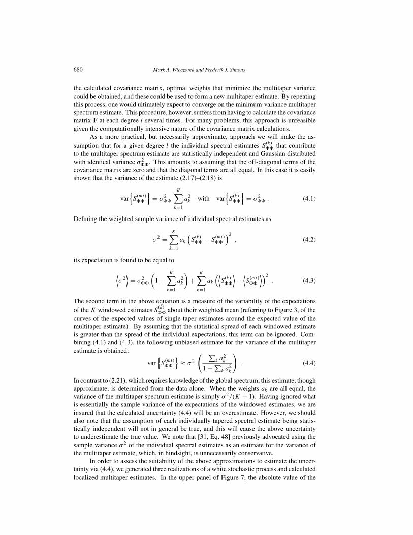
680 Mark A. Wieczorek and Frederik J. Simons
the calculated covariance matrix, optimal weights that minimize the multitaper variancecould be obtained, and these could be used to form a new multitaper estimate. By repeatingthis process, one would ultimately expect to converge on the minimum-variance multitaperspectrum estimate. This procedure, however, suffers from having to calculate the covariancematrix F at each degree l several times. For many problems, this approach is unfeasiblegiven the computationally intensive nature of the covariance matrix calculations.
As a more practical, but necessarily approximate, approach we will make the as-sumption that for a given degree l the individual spectral estimates S
(k)�� that contribute
to the multitaper spectrum estimate are statistically independent and Gaussian distributedwith identical variance σ 2
��. This amounts to assuming that the off-diagonal terms of thecovariance matrix are zero and that the diagonal terms are all equal. In this case it is easilyshown that the variance of the estimate (2.17)–(2.18) is
var{S
(mt)��
}= σ 2
��
K∑k=1
a2k with var
{S
(k)��
}= σ 2
�� . (4.1)
Defining the weighted sample variance of individual spectral estimates as
σ 2 =K∑
k=1
ak
(S
(k)�� − S
(mt)��
)2, (4.2)
its expectation is found to be equal to
⟨σ 2
⟩= σ 2
��
(1 −
K∑k=1
a2k
)+
K∑k=1
ak
(⟨S
(k)��
⟩−
⟨S
(mt)��
⟩)2. (4.3)
The second term in the above equation is a measure of the variability of the expectationsof the K windowed estimates S
(k)�� about their weighted mean (referring to Figure 3, of the
curves of the expected values of single-taper estimates around the expected value of themultitaper estimate). By assuming that the statistical spread of each windowed estimateis greater than the spread of the individual expectations, this term can be ignored. Com-bining (4.1) and (4.3), the following unbiased estimate for the variance of the multitaperestimate is obtained:
var{S
(mt)��
}≈ σ 2
( ∑k a2
k
1 − ∑k a2
k
). (4.4)
In contrast to (2.21), which requires knowledge of the global spectrum, this estimate, thoughapproximate, is determined from the data alone. When the weights ak are all equal, thevariance of the multitaper spectrum estimate is simply σ 2/(K − 1). Having ignored whatis essentially the sample variance of the expectations of the windowed estimates, we areinsured that the calculated uncertainty (4.4) will be an overestimate. However, we shouldalso note that the assumption of each individually tapered spectral estimate being statis-tically independent will not in general be true, and this will cause the above uncertaintyto underestimate the true value. We note that [31, Eq. 48] previously advocated using thesample variance σ 2 of the individual spectral estimates as an estimate for the variance ofthe multitaper estimate, which, in hindsight, is unnecessarily conservative.
In order to assess the suitability of the above approximations to estimate the uncer-tainty via (4.4), we generated three realizations of a white stochastic process and calculatedlocalized multitaper estimates. In the upper panel of Figure 7, the absolute value of the

Minimum-Variance Multitaper Spectral Estimation on the Sphere 681
difference between the multitaper estimate and its expectation based on the known inputspectrum is shown as a function of degree l and number of tapers K for the three real-izations. As is readily seen, the difference between the two almost everywhere decreaseswith increasing number of employed localization windows. Furthermore, comparison withFigure 5 shows that the difference between the two is compatible with the expected uncer-tainty of the multitaper estimate. The bottom panel plots the uncertainty of the multitaperestimate using (4.4), and this is seen to be generally comparable to the difference betweenthe multitaper expectation and single realization in the upper panel. Nevertheless, it shouldbe noted that this estimation of the uncertainty underestimates the true value as shown inFigure 5 by a small factor. This is most likely a result of the fact that the individual spectralestimates are not uncorrelated as we assumed in deriving (4.4).
30
40
50
60
70
80
90
100
Deg
ree
5 10 15 20 25 30
K
30
40
50
60
70
80
90
100
Deg
ree
5 10 15 20 25 30
K
5 10 15 20 25 30
K
5 10 15 20 25 30
K
5 10 15 20 25 30
K
0.05
0.10
0.15
0.20
0.25
0.30
Diff
eren
ce
5 10 15 20 25 30
K
0.05
0.10
0.15
0.20
0.25
0.30
U
ncer
tain
ty
FIGURE 7 Difference and estimated uncertainty for three multitaper realizations of a white stochastic process.(top) Absolute value of the difference between the known multitaper spectrum expectation and the single realizationof the multitaper estimate. (bottom) The estimated uncertainty of the multitaper spectrum estimate calculatedfrom (4.4) using equal weights. Between 2 and 34 tapers were used in generating the multitaper estimates, thetapers were constructed using θ0 = 30◦ and L = 29, and the data were localized at the North pole. For comparisonpurposes, the color bars possess the same range as those in Figure 5.
Finally, we note that it is possible under certain circumstances to invert for the globalpower spectrum using (2.19) combined with knowledge of the multitaper spectral estimatesand their uncertainties. As shown in [31], this equation can be written in matrix notation as⟨
S(mt)��
⟩= M(mt) Sff , (4.5)
where S(mt)�� is a vector containing the L�� + 1 multitaper spectral estimates, Sff is a
vector containing the L�� + L + 1 elements of the global power spectrum, and M(mt) isan (L�� + 1) × (L�� + L + 1) matrix that maps the latter into the former. Assigning the

682 Mark A. Wieczorek and Frederik J. Simons
index 0 to the first row and column of M, the elements are given by
M(mt)ij =
L∑l=0
K∑k=1
ak S(k)hh (l)
(Ci0
l0j0
)2. (4.6)
The individual linear equations of (4.5) could be weighted by the measurement uncertaintiesby dividing each row of S(mt)
�� and M(mt) by the multitaper standard deviation obtainedfrom (4.4).
Inverting M(mt) to obtain Sff from S(mt)�� is an underdetermined inversion problem,
as the dimension of Sff will always be greater than that of S(mt)�� , and M(mt) is never full-
rank. Hence, most of our attempts to invert (4.5) for the global power spectrum, usinga variety of linear techniques, have been unsatisfactory for this example. For instance,choosing that solution for which the norm of Sff is minimized yielded a power spectrumwith both positive and negative values, a situation that is clearly unphysical. Truncating thematrix M to be square yielded similar results. A nonnegative least squares inversion [13,Chap. 23] yielded a solution for which the majority of the Sff (l) were zero. One methodthat did yield acceptable results was to assume that Sff was constant in bins of width�l. However, for the problem at hand, �l was required to be greater than about 15 inorder to obtain positive values with reasonable variances. More sophisticated nonlinearand Monte Carlo techniques that utilize positivity constraints and upper and lower boundsare worth investigating. Alternatively, one could parametrize the global power spectrumby a smoothly varying function (such as a power law) and invert for the parameter valuesthat best fit the observed multitaper spectral estimates. A maximum-likelihood inversionapproach is described in [4] and [8].
5. Concluding Remarks
In this study, we have demonstrated how the global power spectrum of a stochastic processon the sphere can be estimated from spatially limited observation domains. In particular,the act of restriction to a certain region can be formulated as a windowing operation, andthe expectation of the windowed power spectrum has been shown to be related to the globalpower spectrum by a convolution-type equation. The best localization windows are thosethat are spatially concentrated in the region of interest, and yet have as small an effectivespectral bandwidth as possible. Solution of a simple optimization problem yields a familyof orthogonal functions, and a multitaper spectrum estimate can be constructed using thosewindows with good spatiospectral localization properties. The multitaper estimate has thebenefits that the data are more evenly weighted and that it has a reduced variance whencompared to single-window estimates. It is straightforward to choose the weights used inconstructing the multitaper estimate in order to minimize the estimation variance.
While much of the theoretical groundwork has been developed for the problem oflocalized spectral estimation on the sphere, several promising lines of future research couldimprove upon the procedure developed in this work. In particular, we have only concernedourselves with localization windows that are solutions to the spherical-cap concentrationproblem [6, 21, 31]. While sufficient for many problems, such as estimating the localizedspectral properties of planetary gravitational fields and topography, more complex local-ization windows might be desired for other applications. The techniques developed hereare easily generalizable to other concentration domains [20, 21], and we do not expect thegeneral character of our results to differ significantly from those presented here.

Minimum-Variance Multitaper Spectral Estimation on the Sphere 683
As a second line of future research, we note that we have restricted ourselves to usingonly a single localization window when calculating the localized cross-power spectrum S
(k)� .
However, as demonstrated in Appendix B, we could have localized each field by a differentwindow to form localized cross-power spectra S
(j,k)� . Using two different windows, up
to K(K + 1)/2 individual cross-power spectral estimates are, in principle, available foranalysis compared to K as used in this study. The covariance properties of these windowsremain to be investigated, as well as whether their use would significantly decrease themultitaper estimation variance.
Of more practical concern are the computational demands to obtain the covariancematrix. Generating the left and right panels of Figure 4 took about 12 hours and 2 daysof dedicated time on a modern desktop computer, respectively. The calculations for Fig-ure 5 took considerably longer, about one month. Clearly, such computations will becomeincreasingly infeasible as the spherical harmonic degree increases, and alternative meanswill eventually be necessary for computing the covariance matrix, optimal weights, anduncertainties. Asymptotic relations for the Clebsch-Gordan coefficients and/or covariancematrix may be used to simplify these numerical computations at high degrees [4].
Finally, we note that most of our discussion has emphasized the quantification of thebias and uncertainty of the multitaper spectrum estimate. However, in practice, one is ofteninstead interested in obtaining an unbiased estimate of the global power spectrum. Whileone can in principle invert (2.19) for this quantity, the standard linear inversion techniquesdiscussed in Section 4 yielded mixed results. More sophisticated nonlinear and MonteCarlo techniques utilizing bounds and positivity constraints may be worth investigating inthis context.
Appendix
A. Real and Complex Spherical Harmonics
The derivations in this study are considerably simplified if complex spherical harmonicsare used. By inserting the identities
cos β = eiβ + e−iβ
2and sin β = eiβ − e−iβ
2i(A.1)
into (2.1), the spherical harmonic expansion of a real function f is expressed as
f (�) =∞∑l=0
l∑m=−l
flmYlm(�)
=∞∑l=0
l∑m=0
[flm
(eimφ + e−imφ
2
)+ fl−m
(eimφ − e−imφ
2i
)]P̄lm(cos θ)
=∞∑l=0
l∑m=0
[eimφ
(flm − ifl−m
2
)+ e−imφ
(flm + ifl−m
2
)]P̄lm(cos θ)
=∞∑l=0
l∑m=−l
f ml Ym
l (�) , (A.2)

684 Mark A. Wieczorek and Frederik J. Simons
where the complex spherical harmonics, Yml , are defined as
Yml (�) = √
2l + 1
√(l − m)!(l + m)! Plm(cos θ) eimφ . (A.3)
Since
Pl −m = (−1)m(l − m)!(l + m)! Plm , (A.4)
the complex harmonics satisfy the identity
Yml
∗(�) = (−1)m Y−m
l (�) , (A.5)
and normalization1
4π
∫�
Yml
∗(�)Ym′
l′ (�) d� = δll′ δmm′ , (A.6)
where the superscript ∗ indicates complex conjugation. To be consistent with the definitionof the real spherical harmonic functions in Section 2.1, the complex harmonics here alsodo not include the Condon-Shortley phase factor of (−1)m that generally appears in thephysics and seismology communities. Regardless, we note that the inclusion or exclusionof this phase will not affect the results presented in this article. The complex coefficientsare related to the real coefficients by
f ml =
(flm − ifl−m)/√
2 if m > 0fl0 if m = 0(−1)m f −m∗
l if m < 0 ,
(A.7)
and by using the orthogonality properties of the spherical harmonics, these can be shownto be related to the real function f by the relation
f ml = 1
4π
∫�
f (�) Yml
∗(�) d� . (A.8)
It is straightforward to show that the total power of a real function f is related to its complexspectral coefficients by a generalization of Parseval’s theorem:
1
4π
∫�
[f (�)]2 d� =∞∑l=0
Sff (l) , (A.9)
where the power spectrum is
Sff (l) =l∑
m=−l
f ml f m
l∗
. (A.10)
Similarly, the cross-power of two real functions f and g is given by
1
4π
∫�
f (�) g(�) d� =∞∑l=0
Sfg(l) , (A.11)
where the cross-power spectrum is
Sfg(l) =l∑
m=−l
f ml gm
l∗
. (A.12)
Minimum-Variance Multitaper Spectral Estimation on the Sphere 685
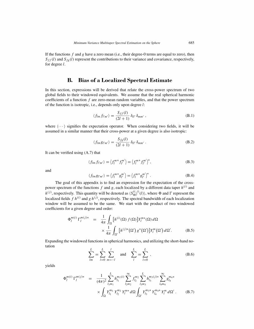
If the functions f and g have a zero mean (i.e., their degree-0 terms are equal to zero), thenSff (l) and Sfg(l) represent the contributions to their variance and covariance, respectively,for degree l.
B. Bias of a Localized Spectral Estimate
In this section, expressions will be derived that relate the cross-power spectrum of twoglobal fields to their windowed equivalents. We assume that the real spherical harmoniccoefficients of a function f are zero-mean random variables, and that the power spectrumof the function is isotropic, i.e., depends only upon degree l:
〈flmfl′m′ 〉 = Sff (l)
(2l + 1)δll′ δmm′ , (B.1)
where 〈· · · 〉 signifies the expectation operator. When considering two fields, it will beassumed in a similar manner that their cross-power at a given degree is also isotropic:
〈flmgl′m′ 〉 = Sfg(l)
(2l + 1)δll′ δmm′ . (B.2)
It can be verified using (A.7) that
〈flmfl′m′ 〉 = ⟨f m
l∗f m′
l′⟩ = ⟨
f ml
∗f m′
l′⟩∗
, (B.3)
and〈flmgl′m′ 〉 = ⟨
f ml
∗gm′
l′⟩ = ⟨
f ml
∗gm′
l′⟩∗
. (B.4)
The goal of this appendix is to find an expression for the expectation of the cross-power spectrum of the functions f and g, each localized by a different data taper h(i) andh(j), respectively. This quantity will be denoted as 〈S(i,j)
� (l)〉, where � and represent thelocalized fields f h(i) and g h(j), respectively. The spectral bandwidth of each localizationwindow will be assumed to be the same. We start with the product of two windowedcoefficients for a given degree and order:
�m(i)l
m(j)∗l = 1
4π
∫�
[h(i)(�) f (�)
]Ym∗
l (�) d�
× 1
4π
∫�′
[h(j)∗(
�′) g∗(�′)]
Yml
(�′) d�′. (B.5)
Expanding the windowed functions in spherical harmonics, and utilizing the short-hand no-tation
L∑lm
=L∑
l=0
l∑m=−l
andL∑l
=L∑
l=0
, (B.6)
yields
�m(i)l
m(j)∗l = 1
(4π)2
L∑l1m1
hm1(i)l1
∞∑l2m2
fm2l2
L∑l3m3
hm3(j)∗l3
∞∑l4m4
gm4∗l4
×∫
�
Ym1l1
Ym2l2
Ym∗l d�
∫�′
Ym3∗l3
Ym4∗l4
Yml d�′ . (B.7)

686 Mark A. Wieczorek and Frederik J. Simons
Averaging this equation over all possible combinations of the random variables gives its ex-pectation:
⟨�
m(i)l
m(j)∗l
⟩= 1
(4π)2
L∑l1m1
hm1(i)l1
L∑l3m3
hm3(j)∗l3
∞∑l2m2
Sfg(l2)
(2l2 + 1)(B.8)
×∫
�
Ym1l1
Ym2l2
Yml
∗d�
∫�′
Ym3∗l3
Ym2l2
∗Ym
l d�′ .
The integral of a triple product of spherical harmonics is real and can be evaluated by awell-known relationship involving Clebsch-Gordan coefficients [27, p. 148]
∫�
Ym1l1
Ym2l2
Ym∗l d� = 4π
√(2l1 + 1)(2l2 + 1)
(2l + 1)Cl0
l10l20 Clml1m1l2m2
, (B.9)
which is nonzero only when the following selection rules are satisfied [27]:
m = m1 + m2 (B.10)
|m| ≤ l; |m1| ≤ l1; |m2| ≤ l2 (B.11)
|l1 − l2| ≤ l ≤ l1 + l2 (B.12)
|l2 − l| ≤ l1 ≤ l2 + l (B.13)
|l − l1| ≤ l2 ≤ l + l1 (B.14)
l1 + l2 + l = even . (B.15)
Combining (B.8) and (B.9), and making use of (A.5), yields
⟨�
m(i)l
m(j)∗l
⟩=
L∑l1m1
hm1(i)l1
L∑l3m3
hm3(j)∗l3
∞∑l2m2
Sfg(l2) (B.16)
×√
(2l1 + 1)(2l3 + 1)
2l + 1Cl0
l10l20 Cl0l30l20 Clm
l1m1l2m2Cl−m
l3−m3l2−m2,
where a phase factor is set equal to unity because of (B.10). We next sum this entireequation over all values of m, employ the symmetry relationship of the Clebsch-Gordancoefficients [27, p. 245]
Cl−ml1−m1l2−m2
= (−1)l1+l2−lClml1m1l2m2
, (B.17)
set a phase factor equal to unity because of (B.15), and rearrange the sum over m2 to obtain
⟨S
(i,j)� (l)
⟩=
L∑l1m1
hm1(i)l1
L∑l3m3
hm3(j)∗l3
∞∑l2
Sfg(l2) (B.18)
×√
(2l1 + 1)(2l3 + 1)
2l + 1Cl0
l10l20 Cl0l30l20
l∑m=−l
l2∑m2=−l2
Clml1m1l2m2
Clml3m3l2m2
.
The final sum over m and m2 is greatly simplified by use of the identity [27, p. 259]
∑α
∑γ
Ccγ
aαbβ Ccγ
aαb′β ′ = (2c + 1)
(2b + 1)δbb′ δββ ′ , (B.19)
Minimum-Variance Multitaper Spectral Estimation on the Sphere 687
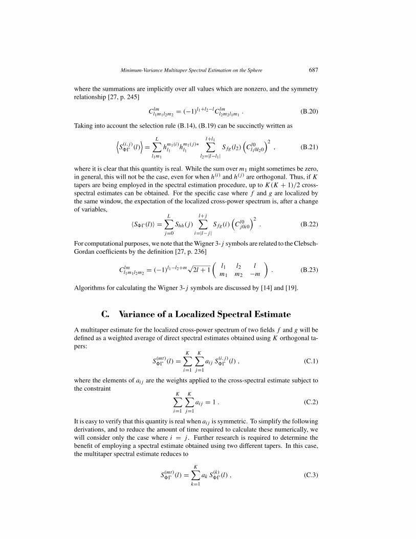
where the summations are implicitly over all values which are nonzero, and the symmetryrelationship [27, p. 245]
Clml1m1l2m2
= (−1)l1+l2−lClml2m2l1m1
. (B.20)
Taking into account the selection rule (B.14), (B.19) can be succinctly written as
⟨S
(i,j)� (l)
⟩=
L∑l1m1
hm1(i)l1
hm1(j)∗l1
l+l1∑l2=|l−l1|
Sfg(l2)(Cl0
l10l20
)2, (B.21)
where it is clear that this quantity is real. While the sum over m1 might sometimes be zero,in general, this will not be the case, even for when h(i) and h(j) are orthogonal. Thus, if K
tapers are being employed in the spectral estimation procedure, up to K(K + 1)/2 cross-spectral estimates can be obtained. For the specific case where f and g are localized bythe same window, the expectation of the localized cross-power spectrum is, after a changeof variables,
〈S� (l)〉 =L∑
j=0
Shh(j)
l+j∑i=|l−j |
Sfg(i)(Cl0
j0i0
)2. (B.22)
For computational purposes, we note that the Wigner 3-j symbols are related to the Clebsch-Gordan coefficients by the definition [27, p. 236]
Clml1m1l2m2
= (−1)l1−l2+m√
2l + 1
(l1 l2 l
m1 m2 −m
). (B.23)
Algorithms for calculating the Wigner 3-j symbols are discussed by [14] and [19].
C. Variance of a Localized Spectral Estimate
A multitaper estimate for the localized cross-power spectrum of two fields f and g will bedefined as a weighted average of direct spectral estimates obtained using K orthogonal ta-pers:
S(mt)� (l) =
K∑i=1
K∑j=1
aij S(i,j)� (l) , (C.1)
where the elements of aij are the weights applied to the cross-spectral estimate subject tothe constraint
K∑i=1
K∑j=1
aij = 1 . (C.2)
It is easy to verify that this quantity is real when aij is symmetric. To simplify the followingderivations, and to reduce the amount of time required to calculate these numerically, wewill consider only the case where i = j . Further research is required to determine thebenefit of employing a spectral estimate obtained using two different tapers. In this case,the multitaper spectral estimate reduces to
S(mt)� (l) =
K∑k=1
ak S(k)� (l) , (C.3)

688 Mark A. Wieczorek and Frederik J. Simons
with the constraintK∑
k=1
ak = 1 . (C.4)
This appendix seeks to determine the variance of such a spectral estimate.We start with the definitions of variance and covariance of complex variables:
var
{N∑
i=1
ai Xi
}=
N∑j=1
N∑k=1
aj cov{Xj , Xk} ak (C.5)
cov{Xj , Xk} = ⟨XjX
∗k
⟩ − 〈Xj 〉⟨X∗
k
⟩. (C.6)
which give the following expression for the variance of (C.3):
var{S
(mt)� (l)
}=
K∑j=1
K∑k=1
aj cov{S
(j)� (l), S
(k)� (l)
}ak . (C.7)
By using the definition of the cross-power spectrum (A.11)–(A.12) with the identity
cov
N∑i=1
Xi,
M∑j=1
Xj
=
N∑i=1
M∑j=1
cov{Xi, Xj } , (C.8)
the covariance of two spectral estimates using tapers j and k can be written as
cov{S
(j)� (l), S
(k)� (l)
}=
l∑m=−l
l∑m′=−l
cov{�
m(j)l
m(j)∗l , �
m′(k)l
m′(k)∗l
}. (C.9)
We proceed by using Isserlis’ theorem [28]
cov{Z1 Z2, Z3 Z4} = cov{Z1, Z3} cov{Z2, Z4} + cov{Z1, Z4} cov{Z2, Z3} , (C.10)
which is valid for zero-mean Gaussian complex random variables Zi . Given that we havepreviously assumed that the coefficients flm and glm have a zero mean, so will the spectralcoefficients of the localized fields �lm and lm. We may then rely on a central-limittheorem [31] to subsequently assume that the localized coefficients will approach a Gaussiandistribution. Alternatively, if we assume that the coefficients of the unwindowed fieldswere Gaussian to begin with, then it is easily shown that the windowed coefficients will beGaussian as well. Under these conditions (C.9) can be written as
cov{S
(j)� (l), S
(k)� (l)
}=
l∑m=−l
l∑m′=−l
(cov
{�
m(j)l , �
m′(k)l
}cov
{
m(j)∗l ,
m′(k)∗l
}
+ cov{�
m(j)l ,
m′(k)∗l
}cov
{
m(j)∗l , �
m′(k)l
}), (C.11)
and it is trivial to generalize (B.17) to show that
cov{�
m(j)l ,
m′(k)l
}=
⟨�
m(j)l
m′(k)∗l
⟩=
L∑l1m1
hm1(j)l1
L∑l3m3
hm3(k)∗l3
∞∑l2m2
Sfg(l2)
×√
(2l1 + 1)(2l3 + 1)
2l + 1Cl0
l10l20 Cl0l30l20 Clm
l1m1l2m2Clm′
l3m3l2m2. (C.12)

Minimum-Variance Multitaper Spectral Estimation on the Sphere 689
For computational purposes, we note that the sums over l2 and m2 are considerably restrictedas a result of the selection rules (B.10)–(B.15), which imply
m2 = m − m1 , (C.13)
m2 = m′ − m3 , (C.14)
m − m1 = m′ − m3 , (C.15)
l1 + l2 + l = even , (C.16)
l3 + l2 + l = even , (C.17)
l1 + l3 = even . (C.18)
The expression for the variance is somewhat simplified when only one field, f , is considered.Noting that ⟨
�m(j)∗l �
m′(k)∗l
⟩=
⟨�
m(j)l �
m′(k)l
⟩∗, (C.19)⟨
�m(j)∗l �
m′(k)l
⟩=
⟨�
m(j)l �
m′(k)∗l
⟩∗, (C.20)
the variance of the multitaper spectral estimate can be written as
var{S
(mt)�� (l)
}=
K∑j=1
K∑k=1
aj Fjk ak , (C.21)
where F implicitly depends upon l and Sff and is given by
Fjk =l∑
m=−l
l∑m′=−l
(∣∣∣⟨�m(j)l �
m′(k)∗l
⟩∣∣∣2 +∣∣∣⟨�m(j)
l �m′(k)l
⟩∣∣∣2)
. (C.22)
Using the negative angular order symmetry relations (A.7) combined with the fact that theabove sums are performed over all values of m, F further simplifies to
Fjk = 2l∑
m=−l
l∑m′=−l
∣∣∣⟨�m(j)l �
m′(k)∗l
⟩∣∣∣2. (C.23)
The covariance matrix is naturally symmetric.Finally, we note that (C.12), and hence the computation of F, can be simplified for the
case where the windows are solutions of the spherical-cap concentration problem [21]. Forthis situation, each window j and k has nonzero real spherical harmonic coefficients only fora single angular order mj and mk , respectively. When the windows are expressed in complexform, this implies that the only nonzero coefficients are for m1 = ±mj , m3 = ±mk ,l1 ≥ |mj | and l3 ≥ |mk|.
D. Correlation of Multitaper Spectral Estimates
It was shown in Appendix B and (2.19) that the expectation of a multitaper spectral estimateat degree l depends upon the global power spectrum within the degree range l ± L, whereL is the bandwidth of the localization windows. It is thus natural to expect that multitaper

690 Mark A. Wieczorek and Frederik J. Simons
spectral estimates separated by less than 2L degrees will be partially correlated. Followingthe methodology presented in Appendix C, this correlation is quantified by the covarianceof the two multitaper spectral estimates, which can be shown to equal
cov{S
(mt)� (l), S
(mt)� (l′)
}=
K∑i=1
K∑j=1
ai F ll′ij aj , (D.1)
where
F ll′ij =
l∑m=−l
l′∑m′=−l′
(cov
{�
m(i)l , �
m′(j)
l′}
cov{
m(i)∗l ,
m′(j)∗l′
}(D.2)
+ cov{�
m(i)l ,
m′(j)∗l′
}cov
{
m(i)∗l , �
m′(j)
l′})
,
and
cov{�
m(i)l ,
m′(j)
l′}
=⟨�
m(i)l
m′(j)∗l′
⟩=
L∑l1m1
hm1(i)l1
L∑l3m3
hm3(j)∗l3
∞∑l2m2
Sfg(l2)
×√
(2l1 + 1)(2l3 + 1)
(2l + 1)(2l′ + 1)Cl0
l10l20 Cl′0l30l20 Clm
l1m1l2m2Cl′m′
l3m3l2m2. (D.3)
If only cross-power spectra of a single function are being considered, the matrix F can beconsiderably simplified to
F ll′ij = 2
l∑m=−l
l′∑m′=−l′
∣∣∣⟨�m(i)l �
m′(j)∗l′
⟩∣∣∣2. (D.4)
Acknowledgements
We thank two anonymous reviewers for comments that helped clarify portions of thismanuscript. Financial support for this work has been provided by the U. S. NationalScience Foundation under Grants EAR-0710860 and EAR-0105387 awarded to FJS atPrinceton University, and by U. K. Natural Environmental Research Council New Investi-gator Award NE/D521449/1 and Nuffield Foundation Grant for Newly Appointed LecturersNAL/01087/G to FJS at University College London. Software for performing the compu-tations in this article can be found on the authors’ web sites. This is IPGP contribution2236.
References[1] Belleguic, V., Lognonné, P., and Wieczorek, M. A. (2005). Constraints on the Martian lithosphere from
gravity and topography data, J. Geophys. Res. 110.
[2] Blakely, R. J. (1995). Potential Theory in Gravity and Magnetic Applications, Cambridge University Press,New York.
[3] Dahlen, F. A. and Tromp, J. (1998). Theoretical Global Seismology, Princeton University Press, Prince-ton, NJ.

Minimum-Variance Multitaper Spectral Estimation on the Sphere 691
[4] Dahlen, F. A. and Simons, F. J. (2007). Spectral estimation on a sphere in geophysics and cosmology, Geo-phys. J. Int., submitted manuscript.
[5] Driscoll, J. R. and Healy, D. M. (1994). Computing Fourier transforms and convolutions on the 2-sphere,Adv. Appl. Math. 15, 202–250.
[6] Grünbaum, F. A., Longhi, L., and Perlstadt, M. (1982). Differential operators commuting with finite con-volution integral operators: Some non-abelian examples, SIAM, J. Appl. Math. 42, 941–955.
[7] Han, S.-C. and Simons, F. J. (2007). Spatiospectral localization of global geopotential fields from GRACEreveals the coseismic gravity change due to the 2004 Sumatra-Andaman earthquake, J. Geophys. Res.,in press.
[8] Hansen, F. K., Górski, K. M., and Hivon, E. (2002). Gabor transforms on the sphere with applications toCMB power spectrum estimation, Mon. Not. R. Astron. Soc. 336, 1304–1328.
[9] Hinshaw, G., Nolta, M. R., Bennett, C. L., Bean, R., Doré, O., Greason, M. R., Halpern, M., Hill, R. S.,Jarosik, N., Kogut, A., Komatsu, E., Limon, M., Odegard, N., Meyer, S. S., Page, L., Peiris, H. V., Spergel,D. N., Tucker, G. S., Verde, L., Weiland, J. L., Wollack, E., and Wright, E. L. (2006). Three-year WilkinsonMicrowave Anisotropy Probe (WMAP) observations: Temperature analysis, arXiv, astro-ph/0603451.
[10] Hivon, E., Górski, K. M., Netterfield, C. B., Crill, B. P., Prunet, S., and Hansen, F. (2002). MASTER of theCosmic Microwave Background anisotropy power spectrum: A fast method for statistical analysis of largeand complex Cosmic Microwave Background data sets, Astroph. J. 567, 2–17.
[11] Holmes, S. A. and Featherstone, W. E. (2002). A unified approach to the Clenshaw summation and therecursive computation of very high degree and order normalised associated Legendre functions, J. Geod.76, 279–299.
[12] Kaula, W. M. (1967). Theory of statistical analysis of data distributed over a sphere, Rev. Geophys. 5,83–107.
[13] Lawson, C. L. and Hanson, R. J. (1995). Solving least squares problems, Classics Appl. Math. SIAM 15.
[14] Luscombe, J. J. and Luban, M. (1998). Simplified recursive algorithm for Wigner 3j and 6j symbols, Phys.Rev. E 57, 7274–7277.
[15] McCoy, E. J., Walden, A. T., and Percival, D. B. (1998). Multitaper spectral estimation of power law pro-cesses, IEEE Trans. Signal Proc. 46, 655–688.
[16] McGovern, P. J., Solomon, S. C., Smith, D. E., Zuber, M. T., Simons, M., Wieczorek, M. A., Phillips, R. J.,Neumann, G. A., Aharonson, O., and Head, J. W. (2002). Localized gravity/topography admittance andcorrelation spectra on Mars: Implications for regional and global evolution, J. Geophys. Res. 107, 5136.
[17] Peebles, P. J. E. (1973). Statistical analysis of catalogs of extragalactic objects, I. Theory, Astroph. J. 185,413–440.
[18] Percival, D. B. and Walden, A. T. (1993). Spectral Analysis for Physical Applications, Multitaper andConventional Univariate Techniques, Cambridge University Press.
[19] Schulten, K. and Gordon, R. G. (1975). Exact recursive evaluation of 3j -coefficients and 6j -coefficientsfor quantum-mechanical coupling of angular momenta, J. Math. Phys. 16, 1961–1970.
[20] Simons, F. J. and Dahlen, F. A. (2006). Spherical Slepian functions and the polar gap in geodesy, Geophys.J. Int. 166, 1039–1061.
[21] Simons, F. J., Dahlen, F. A., and Wieczorek, M. A. (2006). Spatiospectral localization on the sphere, SIAMRev. 48, 504–536.
[22] Simons, M., Solomon, S. C., and Hager, B. H. (1997). Localization of gravity and topography: Constraintson the tectonics and mantle dynamics of Venus, Geophys. J. Int. 131, 24–44.
[23] Slepian, D. and Pollak, H. O. (1960). Prolate spheroidal wave functions, Fourier analysis and uncertainty— I, Bell Syst. Tech. J. 40, 43–63.
[24] Slepian, D. (1983). Some comments on Fourier-analysis, uncertainty and modeling, SIAM Rev. 25, 379–393.
[25] Spergel, D. N., Bean, R., Doré, O., Nolta, M. R., Bennett, C. L., Hinshaw, G., Jarosik, N., Komatsu, E.,Page, L., Peiris, H. V., Verde, L., Barnes, C., Halpern, M., Hill, R. S., Kogut, A., Limon, M., Meyer, S. S.,Odegard, N., Tucker, G. S., Weiland, J. L., Wollack, E., and Wright, E. L. (2006). Wilkinson MicrowaveAnisotropy Probe (WMAP) three year results: Implications for cosmology, arXiv, astro-ph/0603449.
[26] Thomson, D. J. (1982). Spectrum estimation and harmonic analysis, Proc. IEEE 70, 1055–1096.
[27] Varshalovich, D. A., Moskalev, A. N., and Khersonskii, V. K. (1988). Quantum theory of angular momen-tum, World Scientific, Singapore.

692 Mark A. Wieczorek and Frederik J. Simons
[28] Walden, A. T., McCoy, E. J., and Percival, D. B. (1994). The variance of multitaper spectrum estimates forreal Gaussian processes, IEEE Trans. Signal Process. 2, 479–482.
[29] Wieczorek, M. A. (2007). Gravity and topography of the terrestrial planets, in Treatise on Geophyics, 10,Eds. Spohn, T. and Schubert, T., Elsevier-Pergamon, Oxford, in press.
[30] Wieczorek, M. A. (2007). Constraints on the composition of the Martian south polar cap from gravity andtopography, Icarus, in press.
[31] Wieczorek, M. A. and Simons, F. J. (2005). Localized spectral analysis on the sphere, Geophys. J. Int. 162,655–675.
Received September 27, 2006
Revision received May 29, 2007
Equipe d’Etudes Spatiales et Planétologie, Institut de Physique du Globe de Paris,94107 Saint Maur, France
e-mail: [email protected]
Department of Earth Sciences, University College of London,Gower Street, London, WC1E 6BT, United Kingdom
andDepartment of Geosciences, Princeton University, Guyot Hall, Princeton, NJ 08544, USA
e-mail: [email protected]