Mining Business Process Variants:Challenges, Scenarios, Algorithms

Chen Lia,, Manfred Reichertb, Andreas Wombacherc

aInformation Systems Group, University of Twente, The Netherlands (lic@cs.utwente.nl) (B)bInstitute of Databases and Information Systems, Ulm University, Germany (manfred.reichert@uni-ulm.de)

cDatabase Group, University of Twente, The Netherlands (a.wombacher@utwente.nl)

Abstract

During the last decade a new generation of process-aware information systems has emerged,which enables process model configurations at buildtime as well as process instance changesduring runtime. Respective adaptations result in a large number of process model variants thatwere derived from the same process model, but slightly differ in structure. Generally, such modelvariants are expensive to configure and maintain. This paper introduces two different scenariosfor learning from process model adaptations and for discovering a reference model out of whichthe variants can be configured with minimum efforts. The first scenario presumes a referenceprocess model and a collection of related process model variants. The goal is to evolve thereference process model such that it structurally fits better to the given variant models. Thesecond scenario comprises a collection of process variants, while the original reference model isunknown; i.e., the goal is to ”merge” these variants into a reference process model. We suggesttwo algorithms that are applicable in both scenarios, but which have their pros and cons. Wesystematically compare the two algorithms and contrast them with conventional process miningtechniques. Our comparison results indicate good performance of both algorithms. Further theyconfirm that specific techniques are needed for learning from past process adaptations. Finally,we present a case study in the automotive industry in which we applied our algorithms.

1. Introduction

In today’s dynamic business world success of an enterprise increasingly depends on its abil-ity to react to environmental changes in a quick, flexible and cost-effective way [1, 2, 3]. Toincrease the flexibility of Process-Aware Information Systems (PAISs) different approaches forstructurally adapting pre-modeled processes exist, e.g., by adding, deleting or moving processactivities [4, 5]. Respective adaptations are not only needed at buildtime for customizing a givenreference process model to a particular context [6, 7], but also become necessary for tailoringprocess instances during runtime in order to deal with exceptional situations and changing needs[8, 4]. As example consider medical guidelines for patient treatment processes [2], which need tobe customized to fit to the particular healthcare environment in which they are used. Additionaladaptations may become necessary when applying such tailored guideline to a particular patient[2]. Generally, respective adaptations lead to large collections of process model variants (pro-cess variants for short) derived from the same process model, but slightly differing in structure[1, 9]. In case studies we conducted in the healthcare domain and in automotive engineering, forexample, we identified scenarios with dozens up to hundreds of variants [10].Preprint submitted to Data & Knowledge Engineering January 15, 2011

Original reference process model S customization & adaptation

mining & learning

mining & learning

Process Repository

Scenario 1: Original reference process model

is known

Discovered reference process model S’

Discovered reference process model S’

Scenario 2: No original reference process model

is available process variant S1 process variant S2process variant S5process variant S3 process variant S4

process variant Sn…

Improving

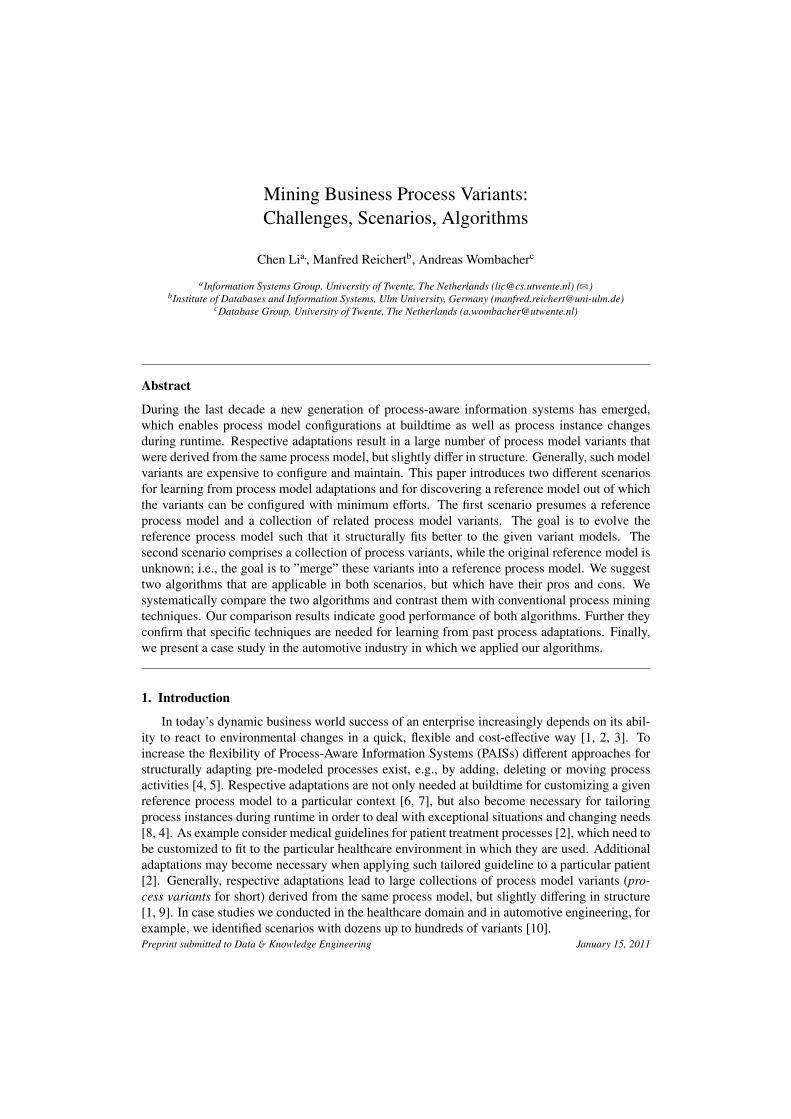
Goal: Discover a (new) reference process model which requires less configuration efforts

Figure 1: Different scenarios for discovering reference process models

1.1. Problem StatementThough considerable efforts have been made to enable process configuration and adaptation

[5, 6, 8, 7], most existing approaches have not utilized information about such structural adap-tations yet [11]. Fig. 1 describes the overall goal of our research. We want to learn from pastprocess model adaptations in order to discover a (new) reference process model covering thegiven variant collection best. By adopting the discovered model in the PAIS, need for futureprocess adaptations and costs for change will decrease. Generally, finding such an improved ref-erence model is by far not trivial when considering control flow patterns like sequence, parallelbranching, conditional branching, and loops. Furthermore, major changes of the current refer-ence process model might be not always preferred due to high implementation costs or for socialreasons. Fig. 1 further differentiates between two fundamental scenarios. In the first scenario theprocess variants are derived by configuring a known reference process model. However, whendiscovering the new reference process model without considering the old one, we might be con-fronted with significant structural differences between old and new reference model. Processengineers should therefore have the flexibility to control to what degree they want to maximallymodify the original reference model to better fit to the given variant collection. Consequently,closeness of the new reference model to the old one and closeness of this model to the givenvariant collection act as ”counterforces”. The second scenario we consider is based on a collec-tion of related process variants, but does not presume any knowledge about the original referenceprocess model these variants were derived from. Here we want to discover a reference processmodel by ”merging” these variants without considering the aforementioned ”counterforces” .

1.2. ContributionBased on the assumptions that process models are block-structured [8, 12] and all activities

in a process model have unique labels1, this paper deals with the following research questions:

1. Given the original reference process model and a collection of related process variants,how can we derive a new reference process model that fits ”better” to these variants? — Inthis scenario we want to control the evolution of the reference process model, i.e., we wantto enable process engineers to control to what degree the new reference model ”differs”from the original one and how ”close” it is to the variant collection.

1The block-structure constraint is discussed in Section 2. Regarding unique activity labeling, we refer to [13] for anapproach that matches activities with different labels.

2

2. Given a collection of process variants without knowledge about the process model theywere derived from, how can we discover a reference process model such that the averagedistance between this reference model and the process variants becomes minimal?

3. Which algorithms foster these two scenarios and what are their commonalities and dif-ferences? How do these algorithms differ from traditional process mining algorithms thatfocus on execution behavior?

As input for our analysis we solely require a collection of process variant models (and areference process model in the first scenario). In particular, we do NOT presume the existenceof process change logs which comprise information about the change patterns that were appliedwhen configuring the variants out of the original reference model [14]. Furthermore we measurethe closeness (or distance) between a reference process model and a related process variant interms of the number of high-level change operations (e.g., to insert, delete or move activities [8])needed to transform the reference process model into the respective variant. As reported in [15]the shorter this distance is, the less the efforts for configuring the variant (i.e., for structurallyadapting the reference process model to derive the variant) are.

In the first scenario, we discover a new reference model by applying a sequence of changeoperations to the original one. Thereby, process engineers have the flexibility to control thesimilarity between original reference model and newly discovered one, i.e., they may specify howmany change operations shall be maximally applied to the old reference model when discoveringthe new one. As benefit of this approach, we can control the efforts for evolving the referenceprocess model. Further, we can avoid Spaghetti-like model structures — a common challenge inthe field of process mining [16, 17]. Finally, in order to support the first scenario we target at anapproach that considers changes, which significantly contribute to reduce the average distancebetween the discovered reference model and the given variant collection, first and less relevantones last (cf. Section 4 for a detailed explanation). In the second scenario, we ”merge” thevariants without considering any original reference process model as ”counterforce”. Based onthis simplification we provide another algorithm which shall perform better than the one designedfor the first scenario. We systematically compare the two mining algorithms. We further comparethem with existing process mining algorithms [18]. The latter aim at discovering a process modelby analyzing the execution behavior of completed process instances as captured in executionlogs [18, 19, 17, 20]. Respective logs typically document the start/end of each activity executionand therefore reflect the behavior of the implemented processes. In principle, process miningtechniques can be applied in our context as well. However, they discover models which coverbehavior best; i.e., their goal is different from ours.

This paper significantly extends our previous work presented in [21]. It handles more processpatterns (e.g., loops), provides more technical and formal details, adds another mining algorithm,and discusses results from a case study. Finally, we compare our algorithms for process variantsmining with existing process mining algorithms based on different criteria.

The remainder of this paper is organized as follows. Section 2 gives background informa-tion and introduces a running example. Section 3 deals with important measures for evaluatingprocess variants in different aspects. Section 4 describes a heuristic algorithm we designed forScenario 1, while Section 5 presents a clustering algorithm for handling Scenario 2. We com-pare the two algorithms with each other as well as with traditional process mining algorithms inSection 6. Results of a case study in the automotive domain are presented in Section 7. Section8 discusses related work, while Section 9 concludes with a summary.

3

2. Backgrounds

A process management system (PrMS) provides generic process support functions and allowsfor separating process logic from application code. For this purpose, the process logic has to beexplicitly defined based on the modeling patterns provided by a process meta model. At runtimethe PrMS then orchestrates the processes according to the defined logic. For each business pro-cess to be supported, a process type represented by a process model S has to be defined. In thispaper, a process model is represented as directed graph, which comprises a set of nodes - eitherrepresenting process steps (i.e., activities) or control connectors (e.g, And-/Xor-Split) – and a setof control edges between them. The latter specify precedence as well as loop backward relations.Furthermore, we presume that process models are block-structured.

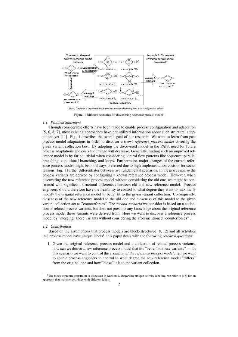
Fig. 2 depicts an example of such a process model. Nodes are represented as rectangles whileprecedence and loop backwards relations are expressed as directed edges of different type. Eachprocess model contains a unique start and a unique end node.2 For control flow modeling thefollowing patterns are available: Sequence, AND-split, AND-join, XOR-split, XOR-join, andLoop [22]. These patterns constitute the core of any process specification language and covermost of the process models we can find in practice [23, 24]. Further, they can be easily mappedto other process execution languages like WS-BPEL as well as to formal languages like PetriNets [25, 26]. Based on these patterns we are able to compose more complex process structuresif required (e.g., an OR-split can be mapped to AND- and XOR-splits [27]).

AndJoinXorJoinAndSplitXorSplitPrecedence LoopStartFlow EndFlowStart End

C

E

FA

BD GStart End

Process model S SequenceLoopConditional branching SequenceSequenceParallel branchingNode types:

Edge types:G (Labeled) activityEndLoop StartLoop

Figure 2: Example of a block-structured process model

Each node a of a process model S may have a label l(a). Such labeled nodes constitute theactivities of S (e.g., activities A and B in Fig. 2). Unlabeled nodes, in turn, represent silentactivities. These have no associated actions and only exist for control flow purpose (e.g., the splitand join nodes in Fig. 2) [28]. In the context our research, for each labeled activity we assumethat its label is unique.3 Regarding the example from Fig. 2, process model S contains 7 normalactivities and 8 silent ones (including the start and end nodes).

We presume that a process model S is block-structured; i.e., activities, sequences, branch-ings, and loops constitute blocks (cf. Fig. 2) with unique start and end nodes4 [29, 30, 31, 12].These blocks may be nested, but must not overlap; i.e., their nesting must be regular [8, 12, 29,31]. Generally a block can be a single activity, a sequence, a parallel branching, a conditional

2For the sake of readability, we omit the start and end node of a process model if its start and end are clear. Forexample, this applies to all process models from Fig. 4.

3Since activity labels are unique we assume that two activities from different process variant models are the same ifthey have same label. Otherwise, we refer to [13] for an approach that matches activities from different process modelsin case they have different labels.

4For example, in Fig. 2 the parallel block comprising activities A and B, and the subsequent activity D togetherconstitute a block.

4

branching, or S itself. In Fig. 2, the grey areas show selected blocks in process model S , and thedifferent grey levels indicate their nesting. In principle, we can consider a block itself as block-structured process model. In the following, we represent each block by a set of activities sincethe block-structure itself can be derived from the overall process model S ; e.g., block {A,B} cor-responds to the parallel block with AND-split and AND-join nodes in S . Similarly, {A}, {A,B,D},{C,F}, and {A,B,C,D,E,F,G} describe selected blocks contained in S .5 The concept of block-structuring has been known from block-structured programming languages for a long time [32],and can be found in process specification language like WS-BPEL and XLANG as well. Further,process management systems with block-structured process modeling language like AristaFlowBPM Suite [33] and CAKE2 [34] emerged, which have been applied to a variety of processesfrom different domains. When compared to unstructured process models, block-structured onesare easier understandable and have lower error probability [35, 36, 37]. If a process model is notblock-structured, in many cases we can transform it into a block-structured one [31, 36, 12, 29].For example, in a case study we analyzed 214 process models from different domains and ex-pressed in different languages (e.g., Event Process Chains, UML Activity Diagrams). Morethan 95% of them were block-structured or could be transformed into a block-structured rep-resentation [38]. Despite the fact that there exist unstructured process models which cannot betransformed into block-structure, we consider our mining algorithms for block-structured processvariant models as highly relevant.

Formally, we define block-structured process model and block as follows:

Definition 1 (Block-structured Process Model and Block).

1. A tuple S = (A, E, AT, ET, l) is called block-structured process model iff:

• A is a set of nodes and AT assigns to each node a ∈ A a node type AT (a) ∈{StartFlow, EndFlow, Normal, AndSplit, AndJoin, XorSplit, XorJoin,

StartLoop, EndLoop}• E ⊆ A × A is a set of directed edges and ET assigns to each edge e ∈ E an edge

type ET (e) ∈ {Precedence,Loop}. Further, n ≺ m :⇔ n directly or indirectlyprecedes m when only considering edges of type precedence.

• Let L be a set of activity labels. l : A→ L is a partial labeling function whichassigns a label l(a) ∈ L to a node a ∈ A.

• S has the block-structure properties as described above (for a formal and precisedescription see Appendix A).

2. Let a1, a2 ∈ A with a1 ≺ a2 or a1 = a2. Let further join(a) be a bijective function to mapeach split/startLoop node a ∈ A with AT (a) ∈ {AndSplit,XorSplit,StartLoop} to itscorresponding join/endLoop node a′ ∈ A with AT (a′) ∈ {AndJoin,XorJoin,EndLoop}.Then: The subgraph of S induced by node set B = {a1, a2}⋃{a ∈ A|a1 ≺ a ∧ a ≺ a2}constitutes a block iff:

• ∀a ∈ B with AT (a) ∈ {AndSplit,XorSplit,StartLoop},⇒ join(a) ∈ B• ∀a ∈ B with AT (a) ∈ {AndJoin,XorJoin,EndLoop},⇒ join−1(a) ∈ B

We do not provide an operational semantics for block-structured process models here, butrefer to [8, 39, 29] instead. As the process patterns used in block-structured process model can

5Here, {C,F} only refers to the sequence structure containing activities C and F. We discuss in Section 3.1 how loopblocks are represented.

5

be easily mapped to WS-BPEL [25] or Petri Nets [22, 26], we could also describe the operationalsemantics of block-structured process models based on these languages. In principle, we canconsider block-structured process models as a subclass of Workflow Nets [26], for which thenet models follow respective structuring constraints. Similar to a Workflow Net, we consider ablock-structured process model S as being sound iff the following properties hold: (1) propercompletion (i.e., when the EndFlow node becomes enabled, all other nodes cannot be enabledanymore), (2) absence of deadlocks (i.e., as long as the EndFlow node has not been enabled,there is no execution situation in which no node is enabled), and (3) absence of dead tasks (i.e.,there exists no node, which can be never enabled). For a formal description of these properties,we refer to [26, 40, 29]. We consider soundness as fundamental requirement any process modelshould satisfy as prerequisite for its proper execution and analysis [40, 8] (see [29, 8, 39, 40, 26]for techniques checking soundness). In the following, P denotes the set of all block-structuredand sound process models.

Based on this, we define the notion of trace as follows:

Definition 2 (Trace). Let S = (A, E, AT, ET, l) ∈ P be a sound and block-structured processmodel. Let further t ≡< a1, a2, . . . , ak > (with ai ∈ A) be a sequence of activities. We denote t astrace of S iff:

• t is valid, i.e., the given execution sequence is producible on S .• t is complete, i.e., a1 is executed immediately after completion of the StartFlow node, and

ak is executed immediately before executing the EndFlow node.

We define TS as the set of all traces that can be produced by process model S .

We only consider traces that log events related to labeled activities, whereas events concern-ing silent activities are excluded (cf. Def. 1). As example consider process model S from Fig.2. Sequences like ABDEG, BADCFG and ABDCFCFCFG constitute valid and complete traces of S .Like most process mining algorithms, we assume that the behavior of process model S can beexpressed in terms of its trace set TS. Note that TS can be an infinite set if S contains loops.

Process change: A process change is accomplished by applying a sequence of high-levelchange operations to the respective process model [8]. Such operations structurally modify agiven process model by altering its set of activities and their order relations. The most relevanthigh-level change operations are insert, delete, and move activity as implemented in the ADEPTchange framework [8]. Table 1 depicts these three change operations and informally describestheir effects on process models. While insert and delete modify the activity set of a process

Change Operation ∆ on S opType subject paramListinsert(S, X,A,B, [sc]) insert X S,A,B, [sc]Effects on S: inserts activity X between activity setsA and B. X is conditionally inserted if [sc] is specified.

delete(S, X) delete X SEffects on S: deletes activity X from S, i.e., X turns into a silent activity.

move(S, X,A,B, [sc]) move X S,A,B, [sc]Effects on S : moves activity X from its original position in S to another position between activitysetsA and B (X is conditionally inserted if [sc] is specified).

Table 1: High-Level Change Operations

6

(a) process model SCEAB D GStart End ACD GStart EndFEBCE FAB D GStart End CE FAB D GStart EndX(b) after insertion Sinstmove (S, A, StartLoop, F)

insert (S, X, startFlow, endFlow, sc) delete(S, F) (d) after move Smov(c) after deletion Sdel

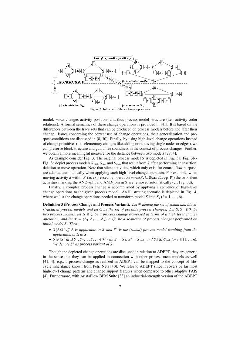
Figure 3: Influence of three change operations

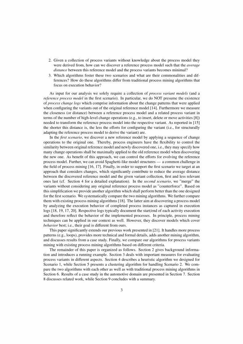
model, move changes activity positions and thus process model structure (i.e., activity orderrelations). A formal semantics of these change operations is provided in [41]. It is based on thedifferences between the trace sets that can be produced on process models before and after theirchange. Issues concerning the correct use of change operations, their generalization and pre-/post-conditions are discussed in [8, 30]. Finally, by using high-level change operations insteadof change primitives (i.e., elementary changes like adding or removing single nodes or edges), wecan preserve block structure and guarantee soundness in the context of process changes. Further,we obtain a more meaningful measure for the distance between two models [28, 4].

As example consider Fig. 3. The original process model S is depicted in Fig. 3a. Fig. 3b -Fig. 3d depict process models S inst, S del and S mov that result from S after performing an insertion,deletion or move operation. Note that silent activities, which only exist for control flow purpose,are adapted automatically when applying such high-level change operation. For example, whenmoving activity A within S (as expressed by operation move(S , A,StartLoop,F)) the two silentactivities marking the AND-split and AND-join in S are removed automatically (cf. Fig. 3d).

Finally, a complex process change is accomplished by applying a sequence of high-levelchange operations to the given process model. An illustrating scenario is depicted in Fig. 4,where we list the change operations needed to transform model S into S i (i = 1, . . . , 6).

Definition 3 (Process Change and Process Variant). Let P denote the set of sound and block-structured process models and let C be the set of possible process changes. Let S , S ′ ∈ P betwo process models, let ∆ ∈ C be a process change expressed in terms of a high level changeoperation, and let σ = 〈∆1,∆2, . . .∆n〉 ∈ C∗ be a sequence of process changes performed oninitial model S . Then:

• S [∆〉S ′ iff ∆ is applicable to S and S ′ is the (sound) process model resulting from theapplication of ∆ to S .

• S [σ〉S ′ iff ∃ S 1, S 2, . . . S n+1 ∈ P with S = S 1, S ′ = S n+1, and S i[∆i〉S i+1 for i ∈ {1, . . . n}.We denote S ′ as process variant of S .

Though the depicted change operations are discussed in relation to ADEPT, they are genericin the sense that they can be applied in connection with other process meta models as well[41, 4]; e.g., a process change as realized in ADEPT can be mapped to the concept of life-cycle inheritance known from Petri Nets [40]. We refer to ADEPT since it covers by far mosthigh-level change patterns and change support features when compared to other adaptive PAIS[4]. Furthermore, with AristaFlow BPM Suite [33] an industrial-strength version of the ADEPT

7

technology emerged, which has been extensively used in a variety of application domains [42].6

Based on Def. 3 and the given change operations, we define distance and bias as follows:

Definition 4 (Bias and Distance). Let S , S ′ ∈ P be two sound and block-structured processmodels. Then: Distance d(S ,S ′) between S and S ′ corresponds to the minimal number of high-level change operations (cf. Table 1) needed to transform S into S ′. We define d(S ,S ′) =

min{|σ|∣∣∣ σ ∈ C∗ ∧ S [σ〉S ′}. Furthermore, a sequence of change operations σ with S [σ〉S ′

and |σ| = d(S ,S ′) is denoted as bias B(S ,S ′) between S and S ′.

The distance between process models S and S ′ corresponds to the minimal number of high-level change operations needed for transforming S into S ′. The corresponding sequence ofchange operations is denoted as bias B(S ,S ′) between S and S ′.7 Usually, distance measures thecomplexity of a process model configuration. As example take Fig. 4. Here, distance betweenmodel S and variant S 4 corresponds to four, since we minimally need to apply four changeoperations to transform S into S 4 [28]. In general, determining the bias and distance betweentwo process models has complexity atNP-hard level [28]. We refer to [28] for an approach thatautomatically computes the distance and bias between two block-structured models without needof a process change log.

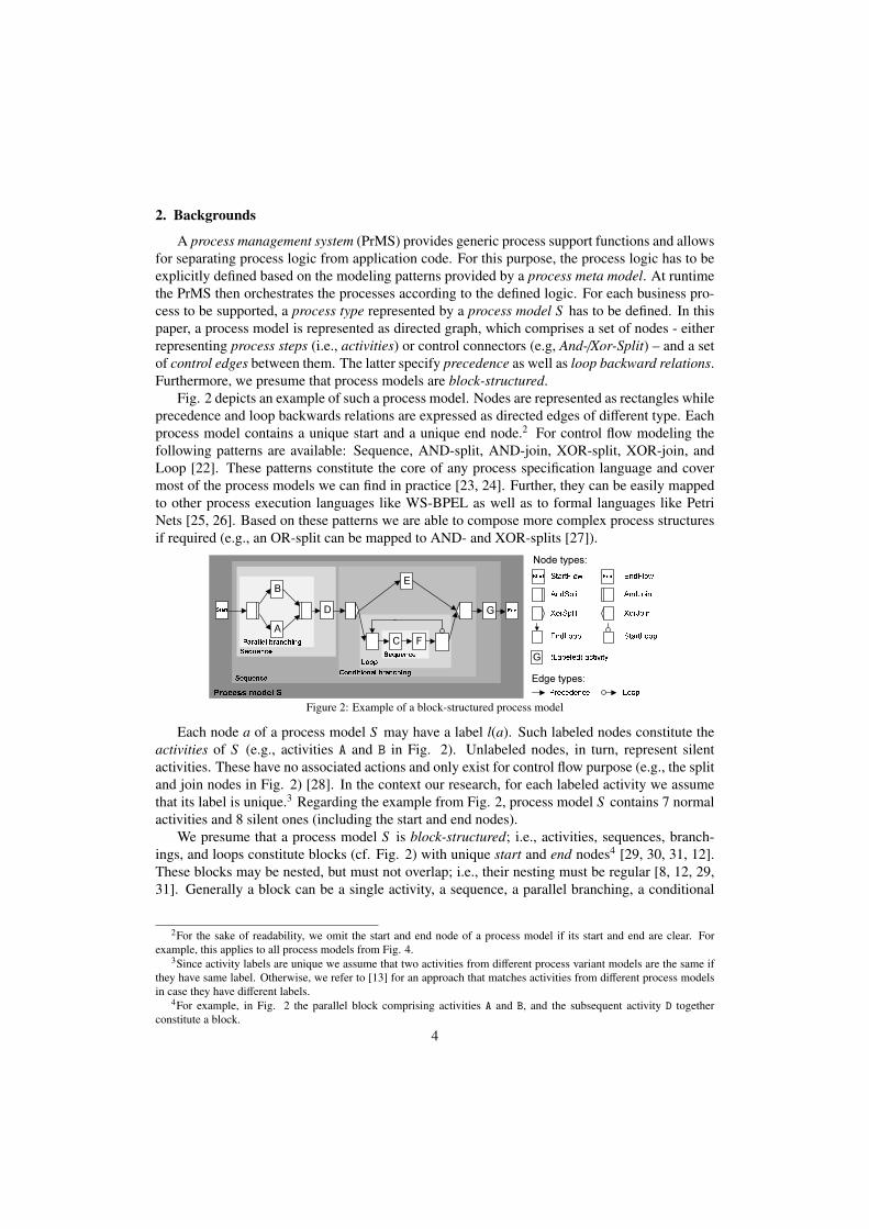
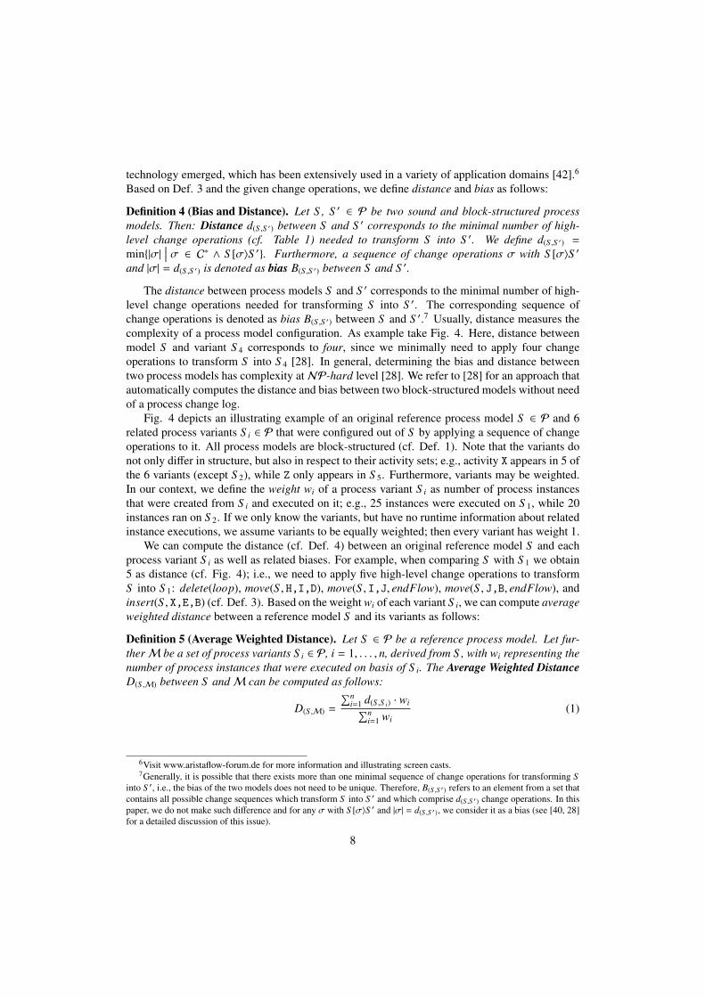
Fig. 4 depicts an illustrating example of an original reference process model S ∈ P and 6related process variants S i ∈ P that were configured out of S by applying a sequence of changeoperations to it. All process models are block-structured (cf. Def. 1). Note that the variants donot only differ in structure, but also in respect to their activity sets; e.g., activity X appears in 5 ofthe 6 variants (except S 2), while Z only appears in S 5. Furthermore, variants may be weighted.In our context, we define the weight wi of a process variant S i as number of process instancesthat were created from S i and executed on it; e.g., 25 instances were executed on S 1, while 20instances ran on S 2. If we only know the variants, but have no runtime information about relatedinstance executions, we assume variants to be equally weighted; then every variant has weight 1.

We can compute the distance (cf. Def. 4) between an original reference model S and eachprocess variant S i as well as related biases. For example, when comparing S with S 1 we obtain5 as distance (cf. Fig. 4); i.e., we need to apply five high-level change operations to transformS into S 1: delete(loop), move(S , H,I,D), move(S , I,J, endFlow), move(S , J,B, endFlow), andinsert(S , X,E,B) (cf. Def. 3). Based on the weight wi of each variant S i, we can compute averageweighted distance between a reference model S and its variants as follows:

Definition 5 (Average Weighted Distance). Let S ∈ P be a reference process model. Let fur-therM be a set of process variants S i ∈ P, i = 1, . . . , n, derived from S , with wi representing thenumber of process instances that were executed on basis of S i. The Average Weighted DistanceD(S ,M) between S andM can be computed as follows:

D(S ,M) =

∑ni=1 d(S ,S i) · wi∑n

i=1 wi(1)

6Visit www.aristaflow-forum.de for more information and illustrating screen casts.7Generally, it is possible that there exists more than one minimal sequence of change operations for transforming S

into S ′, i.e., the bias of the two models does not need to be unique. Therefore, B(S ,S ′) refers to an element from a set thatcontains all possible change sequences which transform S into S ′ and which comprise d(S ,S ′) change operations. In thispaper, we do not make such difference and for any σ with S [σ〉S ′ and |σ| = d(S ,S ′), we consider it as a bias (see [40, 28]for a detailed discussion of this issue).

8

Process configurationoriginal reference model

S1 S2S3 S4S5 S6E Y B JGI HC Z D

AFX

GE BAF IX JDCH

GY HC D BIE JAFX

AF IE BY

JGC H

E BY

JGI H C DAFX

XorSplitXorJoin

S

Weight: w1 = 25Weight: w3 = 10Weight: w5 = 20

Weight: w2 = 20Weight: w4 = 15Weight: w6 = 10 PrecdenceLoop

GE BI JAFC D HAndSplitAndJoin

Average weighted distance = 4.85 change / instance

GH C DE B IJAFX

d(S,S5)= 5< insert(S, Y, {A,F}, B), insert(S, X, E, Y), insert(X, Z, C, D), delete (loop), move (S, J, B, endFlow) >B(S,S5)=Bias:Distance: d(S,S6)= 5< insert(S, X, E, B), insert(S, Y, startFlow, B), delete (loop), move (S, J, B, endFlow), move (S, H, I, C) >B(S,S6)=Bias:Distance: Distance: d(S,S3)= 5< delete (loop), move(S, J, {A,F}, B), insert(S, X, E, J), Insert (S, Y, startFlow, I), move(S, I, D, H) >B(S,S3)=Bias: d(S,S4)= 4< move(S, H, startFlow, I), insert(S, X, E, B), move (S, I, B, endFlow), move (S, J, B, endFlow, con) >B(S,S4)=Bias:Distance: Distance: d(S,S1)= 5< delete (loop), move (S, H, I, D), move(S, I, J, endFlow),move (S, J, B, endFlow), insert(S, X, E, B) >Bias: B(S,S1)= d(S,S2)= 5< insert(S, Y, E, B, con), delete (loop), move(S, C, startFlow, I), move (S, J, B, endFlow), move (S, I, D, H) >B(S,S2)=Bias:Distance:

EndLoopStartLoop

D

Figure 4: An illustrating example of a reference process model and related process variants

The complexity to compute average weighted distance is NP-hard since the complexity tocompute the distance between two variants is NP-hard (cf. Def. 4). Regarding our examplefrom Fig. 4, the distance between S and S 4 is 4, while the distances between S and S i (i , 4)correspond to 5. When considering variant weights, we obtain as average weighted distance:(5×25+5×20+5×10+4×15+5×20+5×10)/(25+20+10+15+20+10) = 4.85. This meanswe need to perform on average 4.85 high-level change operations to configure a process variantS i (and related instance respectively) out of reference process model S . Generally, averageweighted distance between reference model and its variants expresses how ”close” they are.

Our goal is to discover a reference model with shorter average weighted distance to a givencollection of (weighted) process variants than the current reference model (Scenario 1), or mini-mal average weighted distance if the original reference model is unknown (Scenario 2).

3. Matrix-based Representation of Process Models and Process Variant Collections

As basic input for our mining algorithms we take a collection of process variants and option-ally the original reference model they were derived from. This section shows how we representthis information. Its use will be discussed in Sections 4 and 5.

3.1. Representing a Block-structured Process Model as Order MatrixThis subsection first introduces process structure trees which provide a unique tree repre-

sentation of block-structured process models [31] (cf. Section 3.1.1). Then we present the con-cept of order matrix which can be uniquely constructed out of a given process structure tree

9

(cf. Section 3.1.3). Consequently, an order matrix also constitutes a unique representation of ablock-structured process model. Representing process models in terms of a matrix is common inareas like process mining [17], process analysis [26] and process change management [28]. Inparticular, a matrix constitutes a mathematical representation which enables advanced analysesand processing options. In our mining algorithms (cf. Sections 4 and 5), we use order matricesas unique representations of block-structured process models.

3.1.1. Process Structure TreeTransforming a block-structured model into a tree representation has its roots in structured

programming and compiler theory [43]. Such transformation is applied, for example, when ana-lyzing block-structured languages like XML or BPEL. In this paper we apply the approach from[31], which can transform a block-structured process model S into a refined process structuretree in linear time. Such refined process structure tree constitutes a unique representation of aprocess model. In the following, we denote it as process structure tree for short.

Definition 6 (Process Structure Tree). A tuple T = (N,C,CT, E, l) is called a process structuretree if the following holds:

• N is a set of nodes.• C is a set of connectors and CT assigns to each connector c ∈ C a connector type

CT (c) ∈ {Seq, AND, XOR, Loop}.• E ⊆ (C ×C)

⋃(C × N) is a set of directed edges.

• For each cp ∈ C with CT (cp) = Seq, its children in the process structure form an order< acp1

, acp2, . . . , acpk

> with acp1, . . . , acpk

∈ N⋃

C and (cp, acp1), . . . , (cp, acpk

) ∈ E. Wedenote acpi

�cp acp jiff i < j.

• Let L be a set of activity labels, l : N → L is a partial labeling function which assignsa label l(n) to a node n ∈ N.

Process model S

(a) (b)

Process structure tree T

C E FAB D GStart EndProcess model S SequenceLoopConditional branching SequenceSequenceParallel branching XOR1Loop1

Seq1AND1 D GA B ESeq2C F τFigure 5: Process Model S and its corresponding process structure tree T

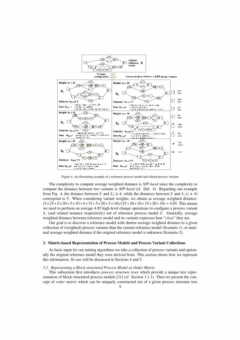
A process structure tree isan ordered tree which consistsof a set of nodes, a set of con-nectors, and a set of directededges linking them. The label-ing function l assigns labels tonodes in a similar way as inDefinition 1. Fig. 5 shows ablock-structured process modelS and its corresponding pro-cess structure tree T . In sucha tree, nodes (represented as

rectangles) correspond to activities while connectors (represented as ellipses) represent their re-lations based on process patterns like Sequence, AND-block, XOR-block, and Loop [22]. Theprecedence relations (expressed by connector Seq) are parsed from left to right; e.g., the AND-block containing activities A and B as well as their connector AND1 precedes activity D since thisblock is on the left. Note that when representing a loop structure within a process structure treeT , we introduce a silent activity τ as direct successor of the respective Loop connector (cf. Fig.

10

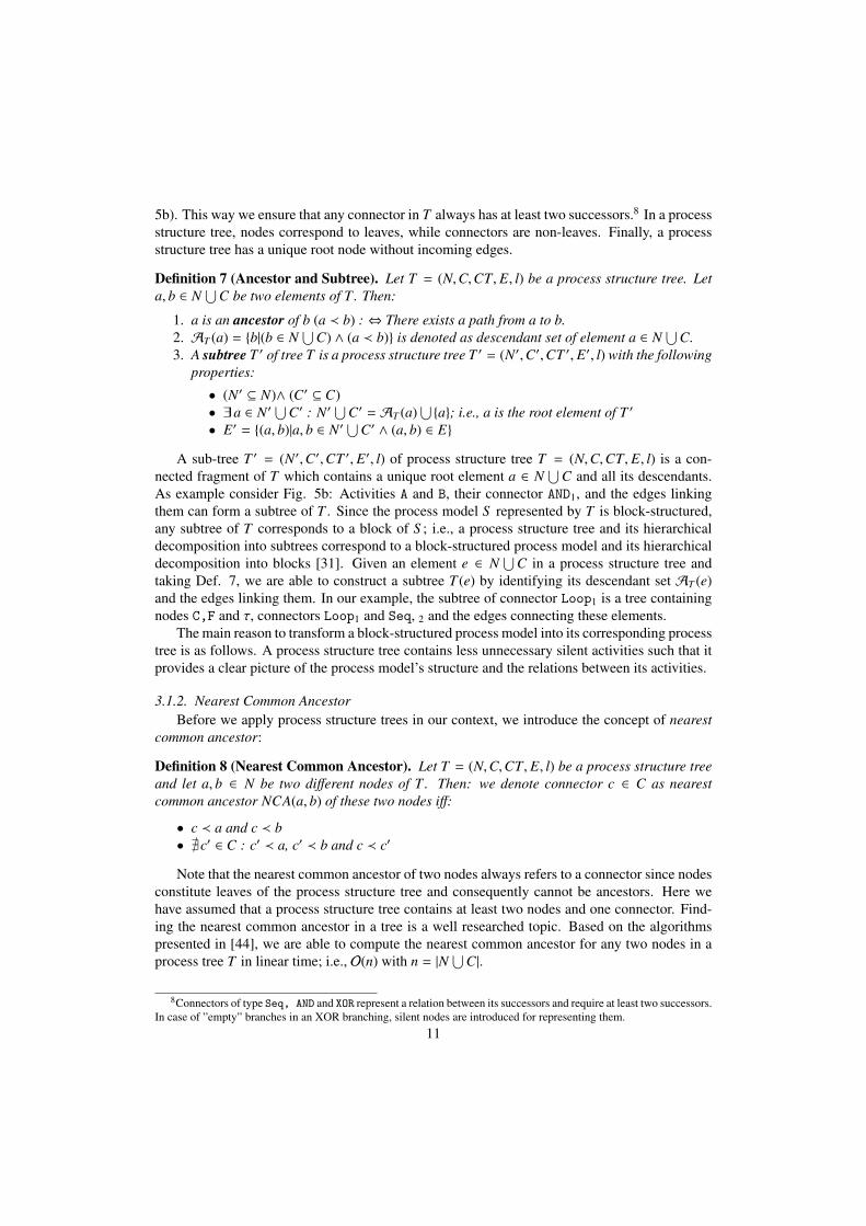
5b). This way we ensure that any connector in T always has at least two successors.8 In a processstructure tree, nodes correspond to leaves, while connectors are non-leaves. Finally, a processstructure tree has a unique root node without incoming edges.

Definition 7 (Ancestor and Subtree). Let T = (N,C,CT, E, l) be a process structure tree. Leta, b ∈ N

⋃C be two elements of T . Then:

1. a is an ancestor of b (a ≺ b) : ⇔ There exists a path from a to b.2. AT (a) = {b|(b ∈ N

⋃C) ∧ (a ≺ b)} is denoted as descendant set of element a ∈ N

⋃C.

3. A subtree T ′ of tree T is a process structure tree T ′ = (N′,C′,CT ′, E′, l) with the followingproperties:

• (N′ ⊆ N)∧ (C′ ⊆ C)• ∃a ∈ N′

⋃C′ : N′

⋃C′ = AT (a)

⋃{a}; i.e., a is the root element of T ′

• E′ = {(a, b)|a, b ∈ N′⋃

C′ ∧ (a, b) ∈ E}A sub-tree T ′ = (N′,C′,CT ′, E′, l) of process structure tree T = (N,C,CT, E, l) is a con-

nected fragment of T which contains a unique root element a ∈ N⋃

C and all its descendants.As example consider Fig. 5b: Activities A and B, their connector AND1, and the edges linkingthem can form a subtree of T . Since the process model S represented by T is block-structured,any subtree of T corresponds to a block of S ; i.e., a process structure tree and its hierarchicaldecomposition into subtrees correspond to a block-structured process model and its hierarchicaldecomposition into blocks [31]. Given an element e ∈ N

⋃C in a process structure tree and

taking Def. 7, we are able to construct a subtree T (e) by identifying its descendant set AT (e)and the edges linking them. In our example, the subtree of connector Loop1 is a tree containingnodes C,F and τ, connectors Loop1 and Seq, 2 and the edges connecting these elements.

The main reason to transform a block-structured process model into its corresponding processtree is as follows. A process structure tree contains less unnecessary silent activities such that itprovides a clear picture of the process model’s structure and the relations between its activities.

3.1.2. Nearest Common AncestorBefore we apply process structure trees in our context, we introduce the concept of nearest

common ancestor:

Definition 8 (Nearest Common Ancestor). Let T = (N,C,CT, E, l) be a process structure treeand let a, b ∈ N be two different nodes of T . Then: we denote connector c ∈ C as nearestcommon ancestor NCA(a, b) of these two nodes iff:

• c ≺ a and c ≺ b• @c′ ∈ C : c′ ≺ a, c′ ≺ b and c ≺ c′

Note that the nearest common ancestor of two nodes always refers to a connector since nodesconstitute leaves of the process structure tree and consequently cannot be ancestors. Here wehave assumed that a process structure tree contains at least two nodes and one connector. Find-ing the nearest common ancestor in a tree is a well researched topic. Based on the algorithmspresented in [44], we are able to compute the nearest common ancestor for any two nodes in aprocess tree T in linear time; i.e., O(n) with n = |N ⋃

C|.

8Connectors of type Seq, AND and XOR represent a relation between its successors and require at least two successors.In case of ”empty” branches in an XOR branching, silent nodes are introduced for representing them.

11

3.1.3. Representing a Process Model as Order MatrixBased on the process structure tree T of a block-structured process model S and the concept

of nearest common ancestor (cf. Def. 8), we can introduce the notion of order matrix, whichuniquely represents a process structure tree and thus a block-structured process model.

Definition 9 (Order matrix). Let S be a block-structured process model and let T = (N,C,CT, E, l)be its process structure tree. A is called order matrix of T with Aaia j representing the order rela-tion between activities ai,a j ∈ N, i , j iff:

• Aaia j = ’1’ iff in T , ai and a j have as nearest common ancestor c ∈ C with CT (c) = Seq;let el and er be two children of c with el �c er and let further Tel and Ter be two subtree ofT with root elements being el and er, ai is contained in the Tel and a j is contained in Ter .

• Aaia j = ’0’ iff in T , ai and a j have as nearest common ancestor c ∈ C with CT (c) = Seq;let el and er be two children of c with el �c er and let further Tel and Ter be two subtree ofT with root elements being el and er, ai is contained in the Ter and a j is contained in Tel .

• Aaia j = ’+’ iff in T , ai and a j have as nearest common ancestor c ∈ C with CT (c) = AND.• Aaia j = ’-’ iff in T , ai and a j have as nearest common ancestor c ∈ C with CT (c) = XOR.• Aaia j = ’L’ iff in T , ai and a j have as nearest common ancestor c ∈ C with CT (c) = Loop.

Order matrix A

AAB

B C D E F G

CDEFG

11 1 1 11 1 1 1 11 11 1 1 1110 0 00 00 0 00 00 0 0 00 0 0 0+

+

-

- --

τ

τ

111-010 0 0L L-

LL‘0’ : successor ‘1’ : predecessor‘+’ : AND-block ‘-’ : XOR-block‘L’ : Loop

(a) (b)

Process structure tree T

XOR1Loop1Seq1AND1 D GA B ESeq2C F τ

Figure 6: Process structure tree T and its corresponding order matrix A

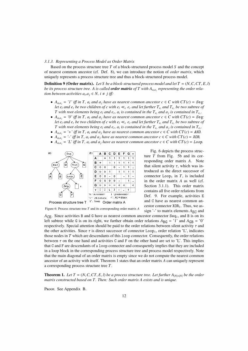
Fig. 6 depicts the process struc-ture T from Fig. 5b and its cor-responding order matrix A. Notethat silent activity τ, which was in-troduced as the direct successor ofconnector Loop1 in T , is includedin the order matrix A as well (cf.Section 3.1.1). This order matrixcontains all five order relations fromDef. 9. For example, activities Eand C have as nearest common an-cestor connector XOR1. Thus, we as-sign ’-’ to matrix elements AEC and

ACE. Since activities B and G have as nearest common ancestor connector Seq1, and B is on itsleft subtree while G is on its right, we further obtain order relations ABG = ’1’ and AGB = ’0’respectively. Special attention should be paid to the order relations between silent activity τ andthe other activities. Since τ is direct successor of connector Loop1, order relation ’L’, indicatesthose nodes in T which are descendants of this loop connector. Consequently, the order relationsbetween τ on the one hand and activities C and F on the other hand are set to ’L’. This impliesthat C and F are descendants of a loop connecter and consequently implies that they are includedin a loop block in the corresponding process structure tree and process model respectively. Notethat the main diagonal of an order matrix is empty since we do not compute the nearest commonancestor of an activity with itself. Theorem 1 states that an order matrix A can uniquely representa corresponding process structure tree T .

Theorem 1. Let T = (N,C,CT, E, l) be a process structure tree. Let further A|N |×|N | be the ordermatrix constructed based on T . Then: Such order matrix A exists and is unique.

Proof. See Appendix B.

12

Since a process structure tree T constitutes a unique representation of a block-structuredprocess model S [31], and T can be uniquely represented by an order matrix A (cf. Theorem1), A is a unique representation of S as well. Consequently, it is sufficient to analyze the ordermatrix of a block-structured process model. We make use of this in Sections 4 and 5. In [45] weprovided algorithms which transform a process model directly to its order matrix and vice versa.

3.2. Representing a Collection of Process Variants as Aggregated Order Matrix

‘0’ : successor‘1’ : predecessor‘+’ : AND-block‘-’ : XOR-block

0 1

+ -L

‘L’ : Loop-block

00 . 1 90 0 . 8 10 00 . 1 70 0 . 8 30 000 01 000 10000 1000 . 2 50 0 . 1 50 . 6 010 00 00 . 8 30 0 . 1 70 000 10 000 10000 10000 10 000 0 . 50 . 5 000 10 000 10000 01000 0 . 8 10 . 1 9000 10 00 . 50 0 . 50 000 10 000 00000 0 . 1 70 . 8 3000 0 . 8 30 . 1 7000 0 . 8 30 . 1 7 000 10 000 10 000 00000 10010 00000 01 000 10 000 00 000 00000 10000 10010 00000 10 00 . 1 70 . 8 3 00 010 00 000 01000 1000 . 60 0 . 1 50 . 2 5H I J X Y Z τ

H

I

J

X

Y

Z

τ

VH I = (0.6, 0.25, 0, 0.1, 0)

‘0’ : 60%‘1’ : 25%‘+’ : 0%‘-’ : 15%‘L’ : 0%

VS1 :25% S 2 :20% S 3 :10% S4 :15% S 5 :20% S 6 :10%H I J X Y Z τ

H 1 - -I 0 - -J - - 0X - - 1YZτ

H I J X Y Z τ

H 0 - -I 1 - -J - - 0XY - - 1Zτ

H I J X Y Z τ

H 0 - - 0I 1 - - 0J - - 0 -X - - 1 -Y 1 1 - -Zτ

H I J X Y Z τ

H - - - 1I - - 0 -J - - 0 -X - 1 1 -YZ

0 - - -τ

H I J X Y Z τ

H 0 - - - 0I 1 - - - 1J - - 0 0 -X - - 1 1 -Y - - 1 0 -Z 1 0 - - -τ

H I J X Y Z τ

H 0 - - -I 1 - - -J - - 0 0X - - 1 -Y - - 1 -Zτ

Order matrices

Aggregated order matrix

Figure 7: Aggregated order matrix based on process variants

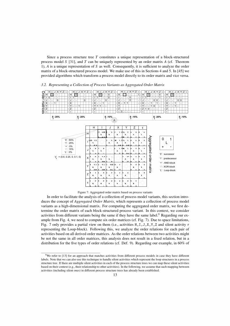
In order to facilitate the analysis of a collection of process model variants, this section intro-duces the concept of Aggregated Order Matrix, which represents a collection of process modelvariants as a high-dimensional matrix. For computing the aggregated order matrix, we first de-termine the order matrix of each block-structured process variant. In this context, we consideractivities from different variants being the same if they have the same label.9 Regarding our ex-ample from Fig. 4, we need to compute six order matrices (cf. Fig. 7). Due to space limitations,Fig. 7 only provides a partial view on them (i.e., activities H,I,J,X,Y,Z and silent activity τrepresenting the Loop-block). Following this, we analyze the order relations for each pair ofactivities based on all derived order matrices. As the order relations between two activities mightbe not the same in all order matrices, this analysis does not result in a fixed relation, but in adistribution for the five types of order relations (cf. Def. 9). Regarding our example, in 60% of

9We refer to [13] for an approach that matches activities from different process models in case they have differentlabels. Note that we can also use this technique to handle silent activities which represent the loop structures in a processstructure tree. If there are multiple silent activities in each of the process structure trees we can map these silent activitiesbased on their context (e.g., their relationship to other activities). In the following, we assume that such mapping betweenactivities (including silent ones) in different process structure trees has already been established.

13

all cases H succeeds I (as in S 2, S 3, S 5 and S 6), in 25% of all cases H precedes I (as in S 1), and in15% of all cases H and I are contained in different branches of an XOR-block (as in S 4) (cf. Fig.7). Generally, for a given variant collection we define the order relation between two activities aand b as 5-dimensional vector Vab = (v0

ab, v1ab, v

+ab, v

−ab, v

Lab). Each vector field corresponds to the

relative frequency of the respective relation type (’0’, ’1’, ’+’, ’-’, or ’L’) as specified in Def. 9.Take our example from Fig. 4 and consider Fig. 7: v1

HI = 0.25 corresponds to the frequency ofall order matrices with activities H and I having order relationship ’1’, i.e., all cases for which Hprecedes I. We obtain VHI = (0.6, 0.25, 0, 0.15, 0).

Definition 10 (Aggregated Order Matrix). Let S i ∈ P, i = 1, 2, . . . , n be a collection of pro-cess variants. Let further Ti = (Ni,Ci,CTi, Ei, li) and Ai be the process structure tree and theorder matrix of S i, and wi be the number of process instances that were executed on S i. The Ag-gregated Order Matrix of all process variants is defined as 2-dimensional matrix Vm×m with m =

|⋃ Ni| and each matrix element va jak = (v0a jak

, v1a jak

, v+a jak

, v−a jak, vL

a jak) being a 5-dimensional vector.

For3 ∈ {0, 1,+,−, L}, element v3a jakexpresses to what percentage, activities a j and ak have order

relation 3 within the given variant collection S 1, . . . , S n. Formally:∀a j, ak ∈ ⋃

Ni, a j , ak :

v3a jak=

∑Aia jak

=′3′ wi∑

a j,ak∈Niwi

. (2)

Fig. 7 partially shows the aggregated order matrix V for the process variants from Fig. 4.Due to space limitations, we only consider order relations for activities H,I,J,X,Y,Z, and silentactivity τ which represents the Loop-block.

3.3. Measuring Activity Frequencies in a Variant Collection

H I J X Y Z τ

H 1 1 0.8 0.6 0.2 0.15

I 1 1 0.8 0.6 0.2 0.15

J 1 1 0.8 0.6 0.2 0.15

X 0.8 0.8 0.8 0.4 0.2 0.15

Y 0.6 0.6 0.6 0.4 0.2 0

Z 0.2 0.2 0.2 0.2 0.2 0

0.15 0.15 0.15 0.15 0 0τ

Figure 8: Coexistence Matrix

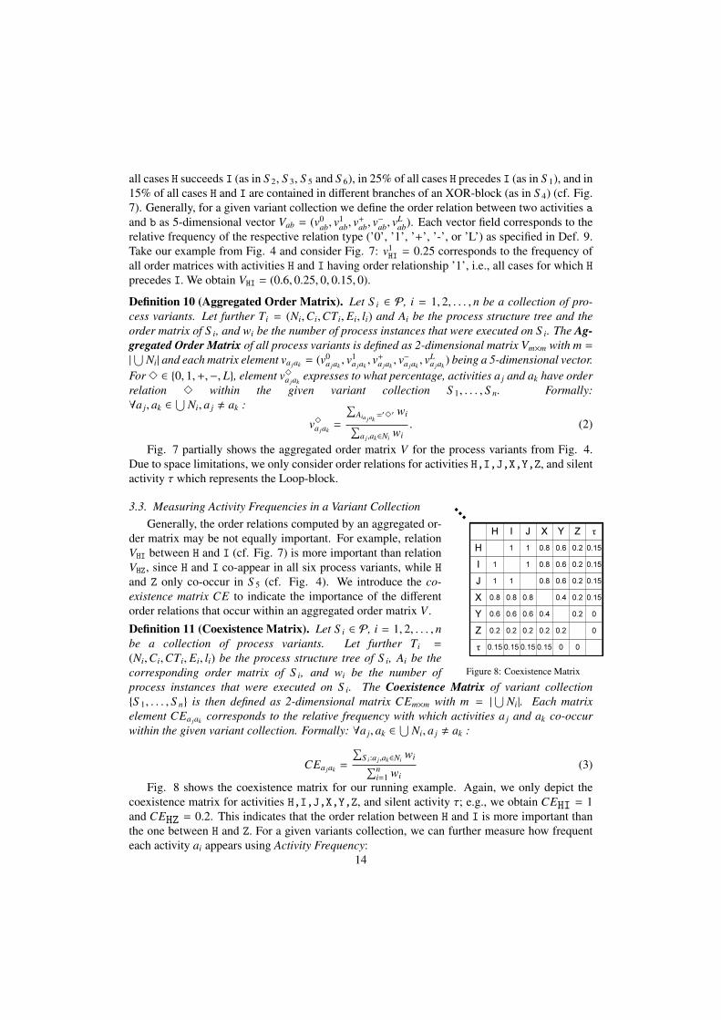
Generally, the order relations computed by an aggregated or-der matrix may be not equally important. For example, relationVHI between H and I (cf. Fig. 7) is more important than relationVHZ, since H and I co-appear in all six process variants, while Hand Z only co-occur in S 5 (cf. Fig. 4). We introduce the co-existence matrix CE to indicate the importance of the differentorder relations that occur within an aggregated order matrix V .

Definition 11 (Coexistence Matrix). Let S i ∈ P, i = 1, 2, . . . , nbe a collection of process variants. Let further Ti =

(Ni,Ci,CTi, Ei, li) be the process structure tree of S i, Ai be thecorresponding order matrix of S i, and wi be the number ofprocess instances that were executed on S i. The Coexistence Matrix of variant collection{S 1, . . . , S n} is then defined as 2-dimensional matrix CEm×m with m = |⋃ Ni|. Each matrixelement CEa jak corresponds to the relative frequency with which activities a j and ak co-occurwithin the given variant collection. Formally: ∀a j, ak ∈ ⋃

Ni, a j , ak :

CEa jak =

∑S i:a j,ak∈Ni

wi∑ni=1 wi

(3)

Fig. 8 shows the coexistence matrix for our running example. Again, we only depict thecoexistence matrix for activities H,I,J,X,Y,Z, and silent activity τ; e.g., we obtain CEHI = 1and CEHZ = 0.2. This indicates that the order relation between H and I is more important thanthe one between H and Z. For a given variants collection, we can further measure how frequenteach activity ai appears using Activity Frequency:

14

Definition 12 (Activity Frequency). Let S i ∈ P, i = 1, 2, . . . , n be a collection of process vari-ants. Let further Ti = (Ni,Ci,CTi, Ei, li) be the process structure tree of S i, Ai be the corre-sponding order matrix, and wi be the number of process instances that were executed on S i. Foreach a j ∈ ⋃n

i=1 Ni, we define g(a j) as relative frequency with which a j appears within the givenvariant collection. Formally:

g(a j) =

∑S i:a j∈Ni

wi∑ni=1 wi

(4)

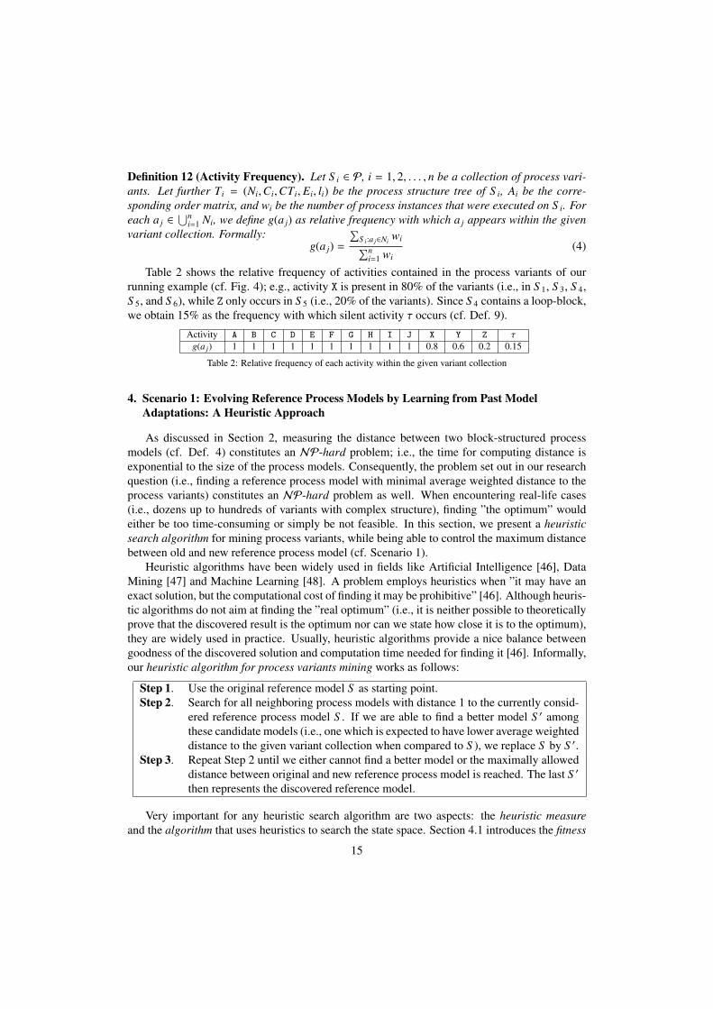
Table 2 shows the relative frequency of activities contained in the process variants of ourrunning example (cf. Fig. 4); e.g., activity X is present in 80% of the variants (i.e., in S 1, S 3, S 4,S 5, and S 6), while Z only occurs in S 5 (i.e., 20% of the variants). Since S 4 contains a loop-block,we obtain 15% as the frequency with which silent activity τ occurs (cf. Def. 9).

Activity A B C D E F G H I J X Y Z τ

g(a j) 1 1 1 1 1 1 1 1 1 1 0.8 0.6 0.2 0.15

Table 2: Relative frequency of each activity within the given variant collection

4. Scenario 1: Evolving Reference Process Models by Learning from Past ModelAdaptations: A Heuristic Approach

As discussed in Section 2, measuring the distance between two block-structured processmodels (cf. Def. 4) constitutes an NP-hard problem; i.e., the time for computing distance isexponential to the size of the process models. Consequently, the problem set out in our researchquestion (i.e., finding a reference process model with minimal average weighted distance to theprocess variants) constitutes an NP-hard problem as well. When encountering real-life cases(i.e., dozens up to hundreds of variants with complex structure), finding ”the optimum” wouldeither be too time-consuming or simply be not feasible. In this section, we present a heuristicsearch algorithm for mining process variants, while being able to control the maximum distancebetween old and new reference process model (cf. Scenario 1).

Heuristic algorithms have been widely used in fields like Artificial Intelligence [46], DataMining [47] and Machine Learning [48]. A problem employs heuristics when ”it may have anexact solution, but the computational cost of finding it may be prohibitive” [46]. Although heuris-tic algorithms do not aim at finding the ”real optimum” (i.e., it is neither possible to theoreticallyprove that the discovered result is the optimum nor can we state how close it is to the optimum),they are widely used in practice. Usually, heuristic algorithms provide a nice balance betweengoodness of the discovered solution and computation time needed for finding it [46]. Informally,our heuristic algorithm for process variants mining works as follows:

Step 1. Use the original reference model S as starting point.Step 2. Search for all neighboring process models with distance 1 to the currently consid-

ered reference process model S . If we are able to find a better model S ′ amongthese candidate models (i.e., one which is expected to have lower average weighteddistance to the given variant collection when compared to S ), we replace S by S ′.

Step 3. Repeat Step 2 until we either cannot find a better model or the maximally alloweddistance between original and new reference process model is reached. The last S ′

then represents the discovered reference model.

Very important for any heuristic search algorithm are two aspects: the heuristic measureand the algorithm that uses heuristics to search the state space. Section 4.1 introduces the fitness

15

function we suggest for measuring the ”quality” of a particular candidate model. Section 4.2 thenintroduces a best-first search algorithm for searching the state space which contains all candidateprocess models.

4.1. Fitness Function

Generally, the fitness function of a heuristic search algorithm should be quickly computable.Since search space often becomes very large, we should be able to make a quick decision whenperforming the search. In our context, average weighted distance (cf. Def. 5) would be not agood choice since the complexity for computing it isNP-hard. Therefore we introduce a fitnessfunction which can be used to approximately measure ”closeness” between a candidate referencemodel and the given variant collection. In particular, this fitness can be computed in polynomialtime. Like in most heuristic search algorithms, the chosen fitness function is a ”reasonableguessing” rather than a precise measurement. Section 4.4 evaluates our choice by investigatingthe correlation between our fitness function and average weighted distance (cf. Def. 5).

4.1.1. Activity CoverageGiven a candidate reference process model S c ∈ P and its process structure tree T =

(Nc,Cc,CTc, Ec, lc) we first measure to what degree activity set Nc covers the activities that oc-cur in the variant collection. Note that we also consider silent activities τk representing loopconnectors in T (cf. Section 3.1.1). We denote this measure as activity coverage AC(S c) of S c.

Definition 13 (Activity coverage). Let S i, i = 1, . . . , n be a collection of process variants, andlet Ti = (Ni,Ci,CTi, Ei, li) be the process structure tree of S i. Let further M =

⋃ni=1 Ni be

the set of activities that are present in at least one of the process structure trees. Let furtherTc = (Nc,Cc,CTc, Ec, lc) be the process structure tree of candidate process model S c. Givenactivity frequency g(a j), for each a j ∈ M the activity coverage AC(S c) of S c is defined as follows:

AC(S c) =

∑a j∈Nc

g(a j)∑a j∈M g(a j)

(5)

Obviously, AC(S c) ∈ [0, 1] holds. Consider Fig. 4 and take the original reference modelS as candidate model. It contains activities A, B, C, D, E, F, G, H, I, J, and τ (whichrepresents the Loop-block). Its activity coverage AC(S ) expresses to what degree S covers theactivities in the given variant collection; we obtain AC(S ) = 10.15

11.8 = 0.860.

4.1.2. Structure Fitting of a Candidate Process ModelsAC(S c) measures how representative the activity set of candidate model S c is in respect to

the given variant collection. However, it does not state how well the structure of S c (i.e., itsorder relations) fits to these variants. We therefore introduce structure fitting S F(S c) as secondmetrics. It measures to what degree S c structurally fits to the given variants collection. For thispurpose, we use the aggregated order matrix (cf. Def. 10) and coexistence matrix (cf. Def. 11).

Since we can represent a candidate process model S c by its corresponding order matrix Ac

(cf. Def. 9), we determine the structure fitting S F(S c) between S c and the variants by measuringhow similar the order matrix Ac and the aggregated order matrix V (representing the variants)are. Take original reference model S in Fig. 4 as candidate process model S c (i.e., S c := S ).Obviously, AHI =’0’ holds, i.e., H succeeds I in S (cf. Fig. 4). Consider now the aggregatedorder matrix V representing the variants (cf. Fig. 7). Here the order relation between H and I isrepresented by the 5-dimensional vector VHI = (0.6, 0.25, 0, 0.15, 0). If we now want to compare

16

how close AHI and VHI are, we first need to build an aggregated order matrix Vc purely basedon our candidate process model S c (S in our case). Trivially, as order relation between H andI in Vc, we obtain Vc

HI = (1, 0, 0, 0, 0). We then compare VHI (which represents the variants)with Vc

HI (which represents the reference model). We use Euclidean metrics f (α, β) to measurecloseness between two vectors α = (x1, x2, ..., xn) and β = (y1, y2, ..., yn):

f (α, β) =α · β|α| · |β| =

∑ni=1 xiyi√∑n

i=1 x2i ·

√∑ni=1 y2

i

∈ [0, 1] (6)

f (α, β) computes the cosine value of the angle θ between vectors α and β in Euclidean space.If f (α, β) = 1 holds, α and β exactly match in their directions; f (α, β) = 0 means, they do notmatch at all. Regarding our running example, we obtain f (VHI,V

cHI) = 0.899. This indicates

high similarity between the order relation of H and I in the candidate process model with theones captured by the variants. Based on Euclidean metrics, which measures similarity betweenthe order relations, and Coexistence matrix CE (cf. Def. 11), which measures importance of theorder relations, we formally define structure fitting S F(S c) of a candidate model S c as follows:

Definition 14 (Structure Fitting). Let S i ∈ P, i = 1, 2, . . . , n be a collection of process variantsand let Ti = (Ni,Ci,CTi, Ei, li) be the corresponding process structure trees. Let further CEbe the coexistence matrix and V be the aggregated order matrix of this variant collection. Forcandidate model S c, let Tc = (Nc,Cc,CTc, Ec, lc) be the corresponding process structure tree,and let m = |Nc| correspond to the number of nodes in Tc. Finally, let Vc be the aggregated ordermatrix of S c. Then structure fitting S F(S c) is defined as follows:

S F(S c) =

∑mj=1

∑mk=1,k, j( f (Va jak ,V

ca jak

) ·CEa jak )

m · (m − 1)∈ [0, 1] (7)

For every pair of activities a j, ak ∈ Nc, j , k, we first compute the similarity of their cor-responding order relations (as captured by V and Vc) in terms of f (Va jak ,V

ca jak

). Second, wedetermine the importance of these order relations by calculating CEa jak . Structure fitting S F(S c)of candidate model S c then equals the average of the similarities multiplied with the importanceof every order relation. Regarding our example from Fig. 4, we obtain S F(S ) = 0.632 whenchoosing S as candidate model.

4.1.3. Fitness FunctionBased on activity coverage AC(S c) (cf. Def. 13) and structure fitting S F(S c) (cf. Def. 14),

we compute fitness Fit(S c) of a candidate model S c as follows:

Definition 15 (Fitness). Let AC(S c) be activity coverage of candidate model S c and S F(S c) beits structure fitting. Fitness Fit(S c) of S c is defined as follows: Fit(S c) = AC(S c) · S F(S c)

As AC(S c) ∈ [0, 1] and S F(S c) ∈ [0, 1] hold, Fit(S c) ∈ [0,1] holds as well. Fit(S c) indicateshow ”close” candidate model S c is to the given variant collection. If Fit(S c) = 1, S c willperfectly fit to the variants; i.e., no further adaptation will be needed. Generally, the higherFit(S c) is, the closer S c is to the variants and the less configuration efforts are required. In ourexample from Fig. 4, original reference model S has Fit(S ) = AC(S ) · S F(S ) = 0.860 · 0.632 =

0.543. As the fitness of candidate model S c is evaluated by multiplying activity coverage AC(S c)with structure fitting S F(S c), a high value for Fit(S c) does not only mean that S c structurally fitswell to the process variants, but also that a reasonable number of activities is considered in thecandidate model.

17

Computing Fit(S c) requires only polynomial time. To be more precise, let S i ∈ P, i =

1, 2, . . . , n be a collection of process variants and let Ti = (Ni,Ci,CTi, Ei, li) be the correspondingprocess structure tree. Let further m = |⋃ Ni|. The complexity for computing Fit(S c) isO(2m2n).

4.2. Constructing the Search Tree

We now show how to find candidate process models. We present a best-first algorithm forconstructing a search tree to find the best candidate model in the search space.

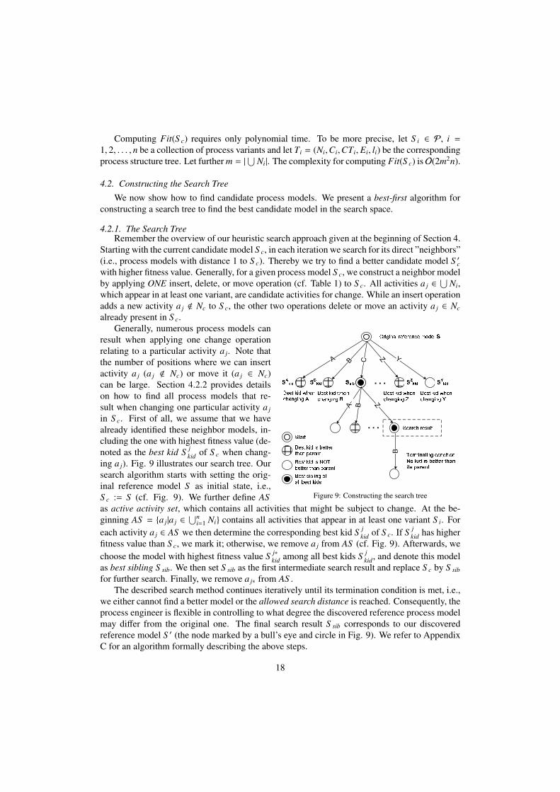
4.2.1. The Search TreeRemember the overview of our heuristic search approach given at the beginning of Section 4.

Starting with the current candidate model S c, in each iteration we search for its direct ”neighbors”(i.e., process models with distance 1 to S c). Thereby we try to find a better candidate model S ′cwith higher fitness value. Generally, for a given process model S c, we construct a neighbor modelby applying ONE insert, delete, or move operation (cf. Table 1) to S c. All activities a j ∈ ⋃

Ni,which appear in at least one variant, are candidate activities for change. While an insert operationadds a new activity a j < Nc to S c, the other two operations delete or move an activity a j ∈ Nc

already present in S c.

SsibSBkidSAkid …

A B C YZ

Best kid when changing AA B Z

…

Best kid when changing Z Best kid when changing YBest kid when changing BBest sibling of all best kids BBest kid is better than parentBest kid is NOT better than parent Terminating condition: No kid is better than its parentStart

Original reference model S

Search resultSZkid SYkid

Figure 9: Constructing the search tree

Generally, numerous process models canresult when applying one change operationrelating to a particular activity a j. Note thatthe number of positions where we can insertactivity a j (a j < Nc) or move it (a j ∈ Nc)can be large. Section 4.2.2 provides detailson how to find all process models that re-sult when changing one particular activity a j

in S c. First of all, we assume that we havealready identified these neighbor models, in-cluding the one with highest fitness value (de-noted as the best kid S j

kid of S c when chang-ing a j). Fig. 9 illustrates our search tree. Oursearch algorithm starts with setting the orig-inal reference model S as initial state, i.e.,S c := S (cf. Fig. 9). We further define ASas active activity set, which contains all activities that might be subject to change. At the be-ginning AS = {a j|a j ∈ ⋃n

i=1 Ni} contains all activities that appear in at least one variant S i. Foreach activity a j ∈ AS we then determine the corresponding best kid S j

kid of S c. If S jkid has higher

fitness value than S c, we mark it; otherwise, we remove a j from AS (cf. Fig. 9). Afterwards, wechoose the model with highest fitness value S j∗

kid among all best kids S jkid, and denote this model

as best sibling S sib. We then set S sib as the first intermediate search result and replace S c by S sib

for further search. Finally, we remove a j∗ from AS .The described search method continues iteratively until its termination condition is met, i.e.,

we either cannot find a better model or the allowed search distance is reached. Consequently, theprocess engineer is flexible in controlling to what degree the discovered reference process modelmay differ from the original one. The final search result S sib corresponds to our discoveredreference model S ′ (the node marked by a bull’s eye and circle in Fig. 9). We refer to AppendixC for an algorithm formally describing the above steps.

18

4.2.2. Changing one Particular ActivitySection 4.2.1 showed how to construct a search tree by comparing best kids S j

kid. We nowdiscuss how to find such best kid S j

kid, i.e., how to find all ”neighbors” of a candidate model S c

by performing one change operation relating to a particular activity a j. Consequently, S jkid is the

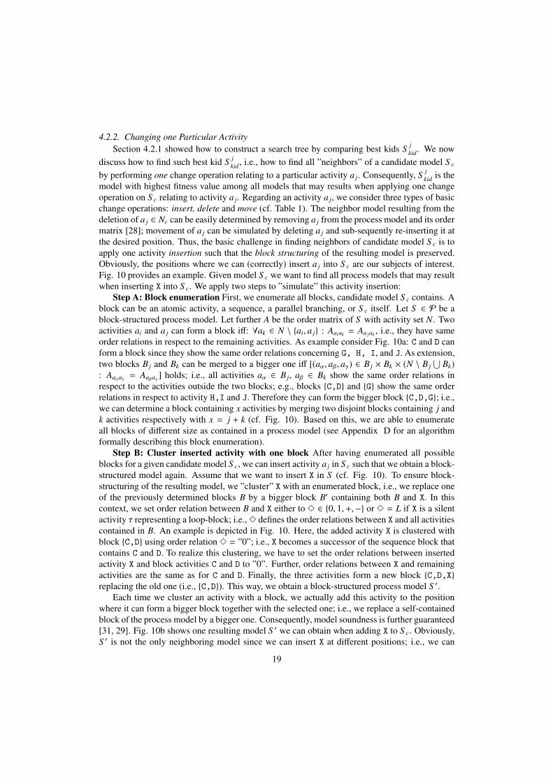
model with highest fitness value among all models that may results when applying one changeoperation on S c relating to activity a j. Regarding an activity a j, we consider three types of basicchange operations: insert, delete and move (cf. Table 1). The neighbor model resulting from thedeletion of a j ∈ Nc can be easily determined by removing a j from the process model and its ordermatrix [28]; movement of a j can be simulated by deleting a j and sub-sequently re-inserting it atthe desired position. Thus, the basic challenge in finding neighbors of candidate model S c is toapply one activity insertion such that the block structuring of the resulting model is preserved.Obviously, the positions where we can (correctly) insert a j into S c are our subjects of interest.Fig. 10 provides an example. Given model S c we want to find all process models that may resultwhen inserting X into S c. We apply two steps to ”simulate” this activity insertion:

Step A: Block enumeration First, we enumerate all blocks, candidate model S c contains. Ablock can be an atomic activity, a sequence, a parallel branching, or S c itself. Let S ∈ P be ablock-structured process model. Let further A be the order matrix of S with activity set N. Twoactivities ai and a j can form a block iff: ∀ak ∈ N \ {ai, a j} : Aaiak = Aa jak , i.e., they have sameorder relations in respect to the remaining activities. As example consider Fig. 10a: C and D canform a block since they show the same order relations concerning G, H, I, and J. As extension,two blocks B j and Bk can be merged to a bigger one iff [(aα, aβ, aγ) ∈ B j × Bk × (N \ B j

⋃Bk)

: Aaαaγ = Aaβaγ ] holds; i.e., all activities aα ∈ B j, aβ ∈ Bk show the same order relations inrespect to the activities outside the two blocks; e.g., blocks {C,D} and {G} show the same orderrelations in respect to activity H,I and J. Therefore they can form the bigger block {C,D,G}; i.e.,we can determine a block containing x activities by merging two disjoint blocks containing j andk activities respectively with x = j + k (cf. Fig. 10). Based on this, we are able to enumerateall blocks of different size as contained in a process model (see Appendix D for an algorithmformally describing this block enumeration).

Step B: Cluster inserted activity with one block After having enumerated all possibleblocks for a given candidate model S c, we can insert activity a j in S c such that we obtain a block-structured model again. Assume that we want to insert X in S (cf. Fig. 10). To ensure block-structuring of the resulting model, we ”cluster” X with an enumerated block, i.e., we replace oneof the previously determined blocks B by a bigger block B′ containing both B and X. In thiscontext, we set order relation between B and X either to 3 ∈ {0, 1,+,−} or 3 = L if X is a silentactivity τ representing a loop-block; i.e.,3 defines the order relations between X and all activitiescontained in B. An example is depicted in Fig. 10. Here, the added activity X is clustered withblock {C,D} using order relation 3 = ”0”; i.e., X becomes a successor of the sequence block thatcontains C and D. To realize this clustering, we have to set the order relations between insertedactivity X and block activities C and D to ”0”. Further, order relations between X and remainingactivities are the same as for C and D. Finally, the three activities form a new block {C,D,X}replacing the old one (i.e., {C,D}). This way, we obtain a block-structured process model S ′.

Each time we cluster an activity with a block, we actually add this activity to the positionwhere it can form a bigger block together with the selected one; i.e., we replace a self-containedblock of the process model by a bigger one. Consequently, model soundness is further guaranteed[31, 29]. Fig. 10b shows one resulting model S ′ we can obtain when adding X to S c. Obviously,S ′ is not the only neighboring model since we can insert X at different positions; i.e., we can

19

a) b) Step A: Enumerating blocks

GI J

C DH {C, D}, {J, H}{C, D, G}{I, C, D, G}, {C, D, G, H}

Blocks containing n activitiesn = 1n = 2n = 3n = 4n = 5n = 6{I}, {G}, {C}, {D}, {J}, {H}{I, C, D, G, J}, {C, D, G, J, H}{I, C, D, G, J, H}

Blocks Enumerate blocksSc: a process model Cluster X with block {C, D} by ◊ = ‘0’ Sc’: one possible resulting model after inserting activity X in ScAc: Order matrix of Sc AS’: Order matrix of Sc’

Step B: Clustering

GI J

C DH

X

Cluster X with block {I, C, D, G, J, H} by ◊ = ‘1’ Cluster X with block {G} by ◊ = ‘+’ Cluster X with block {J, H} by ◊ = ‘-‘Some neighboring models that result when inserting X into Scc)

Cluster X with block {C, D} by ◊ = ‘L’ (only if X is a silent activity τ)

C D G H I JCDGHIJ1 1 11111 1111 1 10 00000 00 0 00 0 0

+++ + Same order relations ◊ = “0”C D G H I JCDGHIJ

+++ + 00000 00 0 00 0 01 10 11 11 11 11 1 1X 1

X

+ 01 1+001

0 011 Copy of block {C,D}

GI J

C DHX

GI J HX

C D

GI J

C DH

XGI

C D HJI

Figure 10: Finding the neighboring models by inserting X into process model S

cluster each block enumerated in Step A with X using any one of the four order relations 3 ∈{0, 1,+,−}, or by ’L’ if X is a silent activity representing a loop-block. In our example from Fig.10, S c contains 14 blocks. Consequently, the number of models that may result when adding Xin S c corresponds to 14 × 4 = 56 (or 14 × 1 = 14 if X is a silent activity); i.e., we can obtain 56(14) potential models. Fig. 10c shows some neighboring models of S c. Note that the resultingmodels are not necessarily unique, i.e., it is possible that some of them are the same. However,this is not a critical issue since Fit(S c) can be quickly computed (cf. Section 4.1); i.e., someredundant information does not significantly decrease algorithm performance.

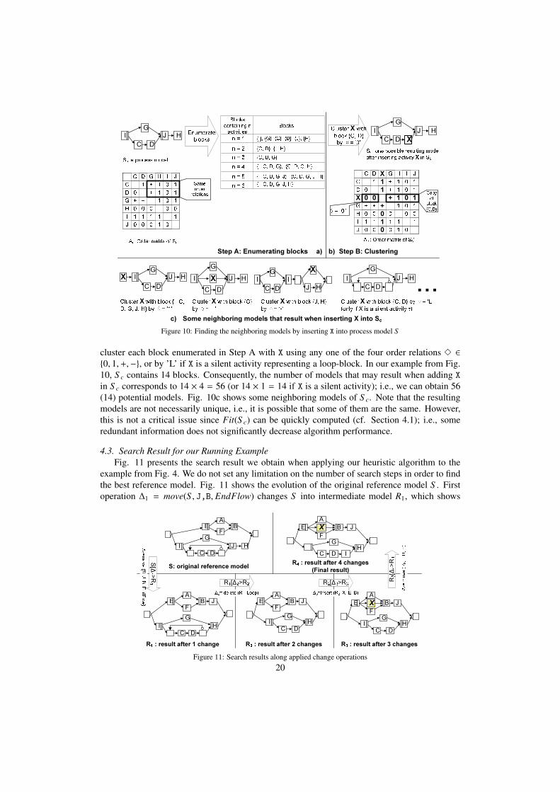
4.3. Search Result for our Running ExampleFig. 11 presents the search result we obtain when applying our heuristic algorithm to the

example from Fig. 4. We do not set any limitation on the number of search steps in order to findthe best reference model. Fig. 11 shows the evolution of the original reference model S . Firstoperation ∆1 = move(S , J,B, EndFlow) changes S into intermediate model R1, which shows

G

E B

I H

AF

C D

J

GE B

H

A

F

C D

JX

I

G

E B

I H

A

F

C D

JX

S: original reference model

∆1=move (S, J, B, EndFlow)

S[∆1>R1R1 : result after 1 change R2 : result after 2 changes

R4 : result after 4 changes (Final result) ∆4= move(R3, I

, D, H)

R 3[∆ 4>R 4GE B

I J

AF

C DH

E BAF

J

GI H

C D

∆3=insert (R2, X, E, B) R2[∆3>R3∆2= delete (R1, Loop) R1[∆2>R2R3 : result after 3 changes

Figure 11: Search results along applied change operations20

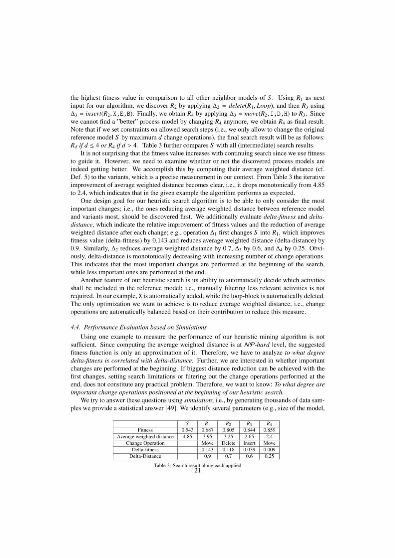
the highest fitness value in comparison to all other neighbor models of S . Using R1 as nextinput for our algorithm, we discover R2 by applying ∆2 = delete(R1, Loop), and then R3 using∆3 = insert(R2, X,E,B). Finally, we obtain R4 by applying ∆3 = move(R2, I,D,H) to R3. Sincewe cannot find a ”better” process model by changing R4 anymore, we obtain R4 as final result.Note that if we set constraints on allowed search steps (i.e., we only allow to change the originalreference model S by maximum d change operations), the final search result will be as follows:Rd if d ≤ 4 or R4 if d > 4. Table 3 further compares S with all (intermediate) search results.

It is not surprising that the fitness value increases with continuing search since we use fitnessto guide it. However, we need to examine whether or not the discovered process models areindeed getting better. We accomplish this by computing their average weighted distance (cf.Def. 5) to the variants, which is a precise measurement in our context. From Table 3 the iterativeimprovement of average weighted distance becomes clear, i.e., it drops monotonically from 4.85to 2.4, which indicates that in the given example the algorithm performs as expected.

One design goal for our heuristic search algorithm is to be able to only consider the mostimportant changes; i.e., the ones reducing average weighted distance between reference modeland variants most, should be discovered first. We additionally evaluate delta-fitness and delta-distance, which indicate the relative improvement of fitness values and the reduction of averageweighted distance after each change; e.g., operation ∆1 first changes S into R1, which improvesfitness value (delta-fitness) by 0.143 and reduces average weighted distance (delta-distance) by0.9. Similarly, ∆2 reduces average weighted distance by 0.7, ∆3 by 0.6, and ∆4 by 0.25. Obvi-ously, delta-distance is monotonically decreasing with increasing number of change operations.This indicates that the most important changes are performed at the beginning of the search,while less important ones are performed at the end.

Another feature of our heuristic search is its ability to automatically decide which activitiesshall be included in the reference model; i.e., manually filtering less relevant activities is notrequired. In our example, X is automatically added, while the loop-block is automatically deleted.The only optimization we want to achieve is to reduce average weighted distance, i.e., changeoperations are automatically balanced based on their contribution to reduce this measure.

4.4. Performance Evaluation based on SimulationsUsing one example to measure the performance of our heuristic mining algorithm is not

sufficient. Since computing the average weighted distance is at NP-hard level, the suggestedfitness function is only an approximation of it. Therefore, we have to analyze to what degreedelta-fitness is correlated with delta-distance. Further, we are interested in whether importantchanges are performed at the beginning. If biggest distance reduction can be achieved with thefirst changes, setting search limitations or filtering out the change operations performed at theend, does not constitute any practical problem. Therefore, we want to know: To what degree areimportant change operations positioned at the beginning of our heuristic search.

We try to answer these questions using simulation; i.e., by generating thousands of data sam-ples we provide a statistical answer [49]. We identify several parameters (e.g., size of the model,

S R1 R2 R3 R4Fitness 0.543 0.687 0.805 0.844 0.859

Average weighted distance 4.85 3.95 3.25 2.65 2.4Change Operation Move Delete Insert Move

Delta-fitness 0.143 0.118 0.039 0.009Delta-Distance 0.9 0.7 0.6 0.25

Table 3: Search result along each applied21

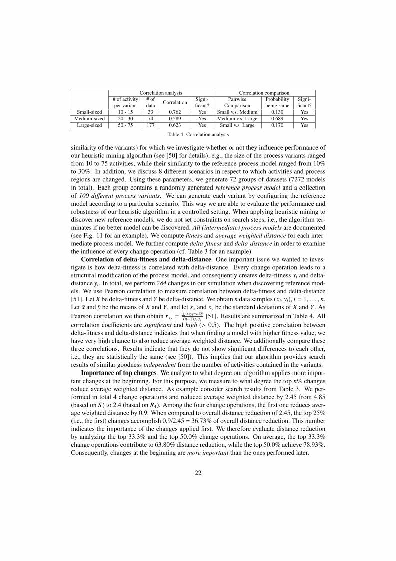
Correlation analysis Correlation comparison# of activity # of Correlation Signi- Pairwise Probability Signi-per variant data ficant? Comparison being same ficant?

Small-sized 10 - 15 33 0.762 Yes Small v.s. Medium 0.130 YesMedium-sized 20 - 30 74 0.589 Yes Medium v.s. Large 0.689 Yes

Large-sized 50 - 75 177 0.623 Yes Small v.s. Large 0.170 Yes

Table 4: Correlation analysis

similarity of the variants) for which we investigate whether or not they influence performance ofour heuristic mining algorithm (see [50] for details); e.g., the size of the process variants rangedfrom 10 to 75 activities, while their similarity to the reference process model ranged from 10%to 30%. In addition, we discuss 8 different scenarios in respect to which activities and processregions are changed. Using these parameters, we generate 72 groups of datasets (7272 modelsin total). Each group contains a randomly generated reference process model and a collectionof 100 different process variants. We can generate each variant by configuring the referencemodel according to a particular scenario. This way we are able to evaluate the performance androbustness of our heuristic algorithm in a controlled setting. When applying heuristic mining todiscover new reference models, we do not set constraints on search steps, i.e., the algorithm ter-minates if no better model can be discovered. All (intermediate) process models are documented(see Fig. 11 for an example). We compute fitness and average weighted distance for each inter-mediate process model. We further compute delta-fitness and delta-distance in order to examinethe influence of every change operation (cf. Table 3 for an example).

Correlation of delta-fitness and delta-distance. One important issue we wanted to inves-tigate is how delta-fitness is correlated with delta-distance. Every change operation leads to astructural modification of the process model, and consequently creates delta-fitness xi and delta-distance yi. In total, we perform 284 changes in our simulation when discovering reference mod-els. We use Pearson correlation to measure correlation between delta-fitness and delta-distance[51]. Let X be delta-fitness and Y be delta-distance. We obtain n data samples (xi, yi), i = 1, . . . , n.Let x and y be the means of X and Y , and let sx and sy be the standard deviations of X and Y . AsPearson correlation we then obtain rxy =

∑xiyi−nxy

(n−1)sx sy[51]. Results are summarized in Table 4. All

correlation coefficients are significant and high (> 0.5). The high positive correlation betweendelta-fitness and delta-distance indicates that when finding a model with higher fitness value, wehave very high chance to also reduce average weighted distance. We additionally compare thesethree correlations. Results indicate that they do not show significant differences to each other,i.e., they are statistically the same (see [50]). This implies that our algorithm provides searchresults of similar goodness independent from the number of activities contained in the variants.

Importance of top changes. We analyze to what degree our algorithm applies more impor-tant changes at the beginning. For this purpose, we measure to what degree the top n% changesreduce average weighted distance. As example consider search results from Table 3. We per-formed in total 4 change operations and reduced average weighted distance by 2.45 from 4.85(based on S ) to 2.4 (based on R4). Among the four change operations, the first one reduces aver-age weighted distance by 0.9. When compared to overall distance reduction of 2.45, the top 25%(i.e., the first) changes accomplish 0.9/2.45 = 36.73% of overall distance reduction. This numberindicates the importance of the changes applied first. We therefore evaluate distance reductionby analyzing the top 33.3% and the top 50.0% change operations. On average, the top 33.3%change operations contribute to 63.80% distance reduction, while the top 50.0% achieve 78.93%.Consequently, changes at the beginning are more important than the ones performed later.

22

5. Scenario 2: Discovering a Reference Process Model by Mining Process Model Variants:A Clustering Approach

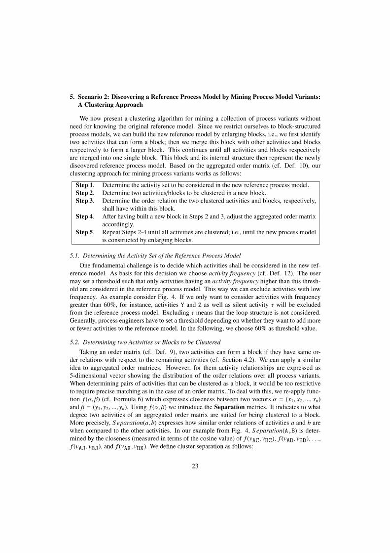
We now present a clustering algorithm for mining a collection of process variants withoutneed for knowing the original reference model. Since we restrict ourselves to block-structuredprocess models, we can build the new reference model by enlarging blocks, i.e., we first identifytwo activities that can form a block; then we merge this block with other activities and blocksrespectively to form a larger block. This continues until all activities and blocks respectivelyare merged into one single block. This block and its internal structure then represent the newlydiscovered reference process model. Based on the aggregated order matrix (cf. Def. 10), ourclustering approach for mining process variants works as follows:

Step 1. Determine the activity set to be considered in the new reference process model.Step 2. Determine two activities/blocks to be clustered in a new block.Step 3. Determine the order relation the two clustered activities and blocks, respectively,

shall have within this block.Step 4. After having built a new block in Steps 2 and 3, adjust the aggregated order matrix

accordingly.Step 5. Repeat Steps 2-4 until all activities are clustered; i.e., until the new process model

is constructed by enlarging blocks.

5.1. Determining the Activity Set of the Reference Process Model

One fundamental challenge is to decide which activities shall be considered in the new ref-erence model. As basis for this decision we choose activity frequency (cf. Def. 12). The usermay set a threshold such that only activities having an activity frequency higher than this thresh-old are considered in the reference process model. This way we can exclude activities with lowfrequency. As example consider Fig. 4. If we only want to consider activities with frequencygreater than 60%, for instance, activities Y and Z as well as silent activity τ will be excludedfrom the reference process model. Excluding τ means that the loop structure is not considered.Generally, process engineers have to set a threshold depending on whether they want to add moreor fewer activities to the reference model. In the following, we choose 60% as threshold value.

5.2. Determining two Activities or Blocks to be Clustered

Taking an order matrix (cf. Def. 9), two activities can form a block if they have same or-der relations with respect to the remaining activities (cf. Section 4.2). We can apply a similaridea to aggregated order matrices. However, for them activity relationships are expressed as5-dimensional vector showing the distribution of the order relations over all process variants.When determining pairs of activities that can be clustered as a block, it would be too restrictiveto require precise matching as in the case of an order matrix. To deal with this, we re-apply func-tion f (α, β) (cf. Formula 6) which expresses closeness between two vectors α = (x1, x2, ..., xn)and β = (y1, y2, ..., yn). Using f (α, β) we introduce the Separation metrics. It indicates to whatdegree two activities of an aggregated order matrix are suited for being clustered to a block.More precisely, S eparation(a, b) expresses how similar order relations of activities a and b arewhen compared to the other activities. In our example from Fig. 4, S eparation(A,B) is deter-mined by the closeness (measured in terms of the cosine value) of f (vAC, vBC), f (vAD, vBD), . . .,f (vAJ, vBJ), and f (vAX, vBX). We define cluster separation as follows:

23

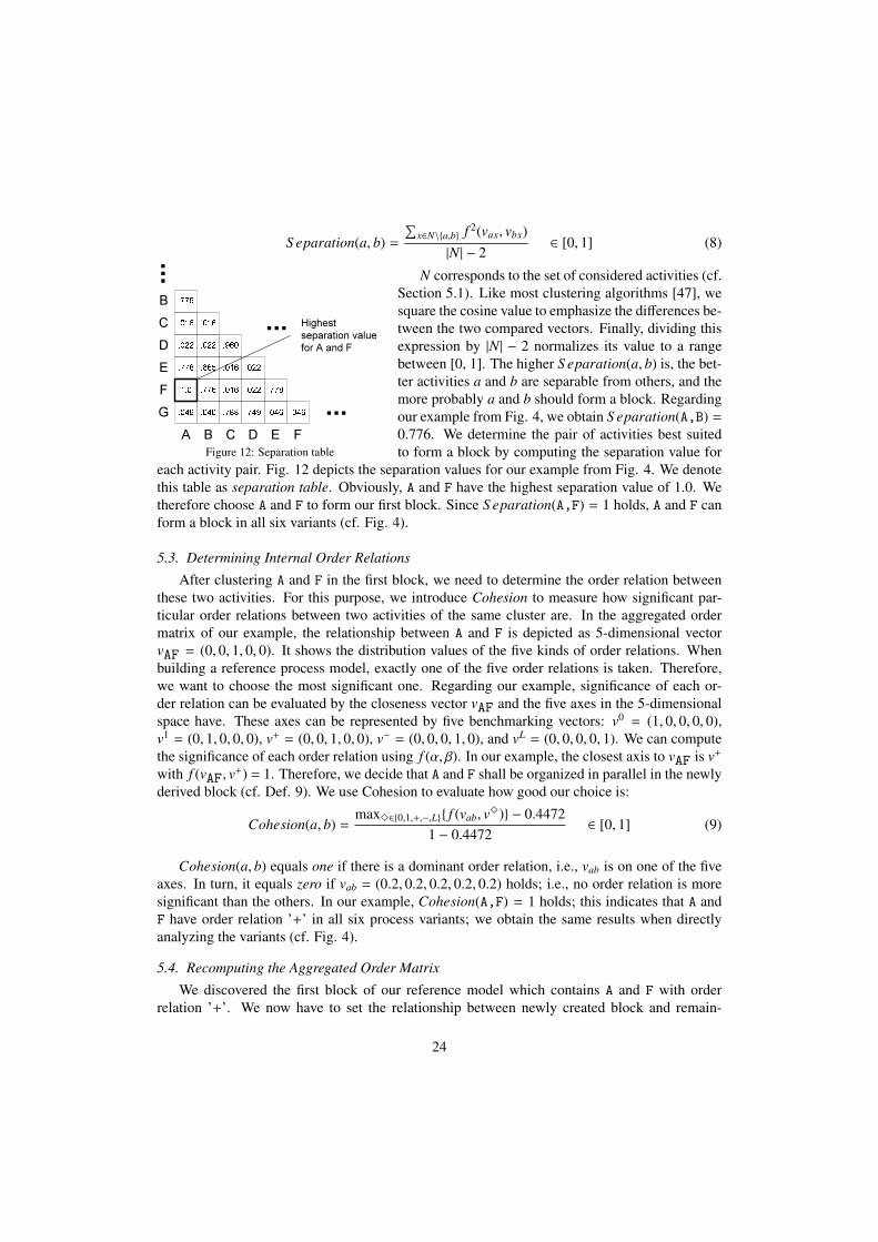
S eparation(a, b) =

∑x∈N\{a,b} f 2(vax, vbx)

|N| − 2∈ [0, 1] (8)

A B C D E F

B .776C .016 .016D .022 .022 .960E .778 .665 .016 .022F 1.0 .776 .016 .022 .778.046 .046 .788 .749 .046 .046G

Highest separation value for A and F

...

...

...

Figure 12: Separation table

N corresponds to the set of considered activities (cf.Section 5.1). Like most clustering algorithms [47], wesquare the cosine value to emphasize the differences be-tween the two compared vectors. Finally, dividing thisexpression by |N| − 2 normalizes its value to a rangebetween [0, 1]. The higher S eparation(a, b) is, the bet-ter activities a and b are separable from others, and themore probably a and b should form a block. Regardingour example from Fig. 4, we obtain S eparation(A,B) =

0.776. We determine the pair of activities best suitedto form a block by computing the separation value for

each activity pair. Fig. 12 depicts the separation values for our example from Fig. 4. We denotethis table as separation table. Obviously, A and F have the highest separation value of 1.0. Wetherefore choose A and F to form our first block. Since S eparation(A,F) = 1 holds, A and F canform a block in all six variants (cf. Fig. 4).

5.3. Determining Internal Order Relations

After clustering A and F in the first block, we need to determine the order relation betweenthese two activities. For this purpose, we introduce Cohesion to measure how significant par-ticular order relations between two activities of the same cluster are. In the aggregated ordermatrix of our example, the relationship between A and F is depicted as 5-dimensional vectorvAF = (0, 0, 1, 0, 0). It shows the distribution values of the five kinds of order relations. Whenbuilding a reference process model, exactly one of the five order relations is taken. Therefore,we want to choose the most significant one. Regarding our example, significance of each or-der relation can be evaluated by the closeness vector vAF and the five axes in the 5-dimensionalspace have. These axes can be represented by five benchmarking vectors: v0 = (1, 0, 0, 0, 0),v1 = (0, 1, 0, 0, 0), v+ = (0, 0, 1, 0, 0), v− = (0, 0, 0, 1, 0), and vL = (0, 0, 0, 0, 1). We can computethe significance of each order relation using f (α, β). In our example, the closest axis to vAF is v+

with f (vAF, v+) = 1. Therefore, we decide that A and F shall be organized in parallel in the newly

derived block (cf. Def. 9). We use Cohesion to evaluate how good our choice is:

Cohesion(a, b) =max3∈{0,1,+,−,L}{ f (vab, v3)} − 0.4472

1 − 0.4472∈ [0, 1] (9)

Cohesion(a, b) equals one if there is a dominant order relation, i.e., vab is on one of the fiveaxes. In turn, it equals zero if vab = (0.2, 0.2, 0.2, 0.2, 0.2) holds; i.e., no order relation is moresignificant than the others. In our example, Cohesion(A,F) = 1 holds; this indicates that A andF have order relation ’+’ in all six process variants; we obtain the same results when directlyanalyzing the variants (cf. Fig. 4).

5.4. Recomputing the Aggregated Order Matrix

We discovered the first block of our reference model which contains A and F with orderrelation ’+’. We now have to set the relationship between newly created block and remain-

24

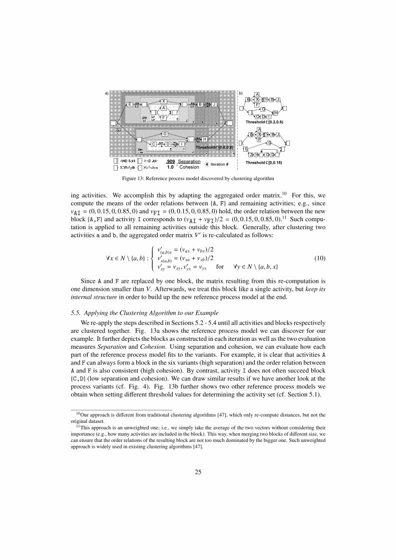
AND-Split AND-JoinXOR-Split XOR-Join .9091.0

SeparationCohesion: 4 Iteration #

G 6DC 7I 8 H93

X 21F

A.9991.0E 4B J 51.01.0.9991.0 .9981.0 .994.997.9091.0 .796.735.864.793 .999.746 10

____ .999E Y

A

FBX J

G HC D I

E YA

FBX J

GI

Z H C D

a) b)

Threshold [0.2,0.6)

Threshold [0,0.15)

Threshold [0.6,0.8)

Figure 13: Reference process model discovered by clustering algorithm

ing activities. We accomplish this by adapting the aggregated order matrix.10 For this, wecompute the means of the order relations between {A, F} and remaining activities; e.g., sincevAI = (0, 0.15, 0, 0.85, 0) and vFI = (0, 0.15, 0, 0.85, 0) hold, the order relation between the newblock {A,F} and activity I corresponds to (vAI + vFI)/2 = (0, 0.15, 0, 0.85, 0).11 Such compu-tation is applied to all remaining activities outside this block. Generally, after clustering twoactivities a and b, the aggregated order matrix V ′ is re-calculated as follows:

∀x ∈ N \ {a, b} :

v′(a,b)x = (vax + vbx)/2v′x(a,b) = (vxa + vxb)/2v′xy = vxy, v′yx = vyx for ∀y ∈ N \ {a, b, x}

(10)

Since A and F are replaced by one block, the matrix resulting from this re-computation isone dimension smaller than V . Afterwards, we treat this block like a single activity, but keep itsinternal structure in order to build up the new reference process model at the end.

5.5. Applying the Clustering Algorithm to our Example

We re-apply the steps described in Sections 5.2 - 5.4 until all activities and blocks respectivelyare clustered together. Fig. 13a shows the reference process model we can discover for ourexample. It further depicts the blocks as constructed in each iteration as well as the two evaluationmeasures Separation and Cohesion. Using separation and cohesion, we can evaluate how eachpart of the reference process model fits to the variants. For example, it is clear that activities Aand F can always form a block in the six variants (high separation) and the order relation betweenA and F is also consistent (high cohesion). By contrast, activity I does not often succeed block{C,D} (low separation and cohesion). We can draw similar results if we have another look at theprocess variants (cf. Fig. 4). Fig. 13b further shows two other reference process models weobtain when setting different threshold values for determining the activity set (cf. Section 5.1).

10Our approach is different from traditional clustering algorithms [47], which only re-compute distances, but not theoriginal dataset.

11This approach is an unweighted one; i.e., we simply take the average of the two vectors without considering theirimportance (e.g., how many activities are included in the block). This way, when merging two blocks of different size, wecan ensure that the order relations of the resulting block are not too much dominated by the bigger one. Such unweightedapproach is widely used in existing clustering algorithms [47].

25

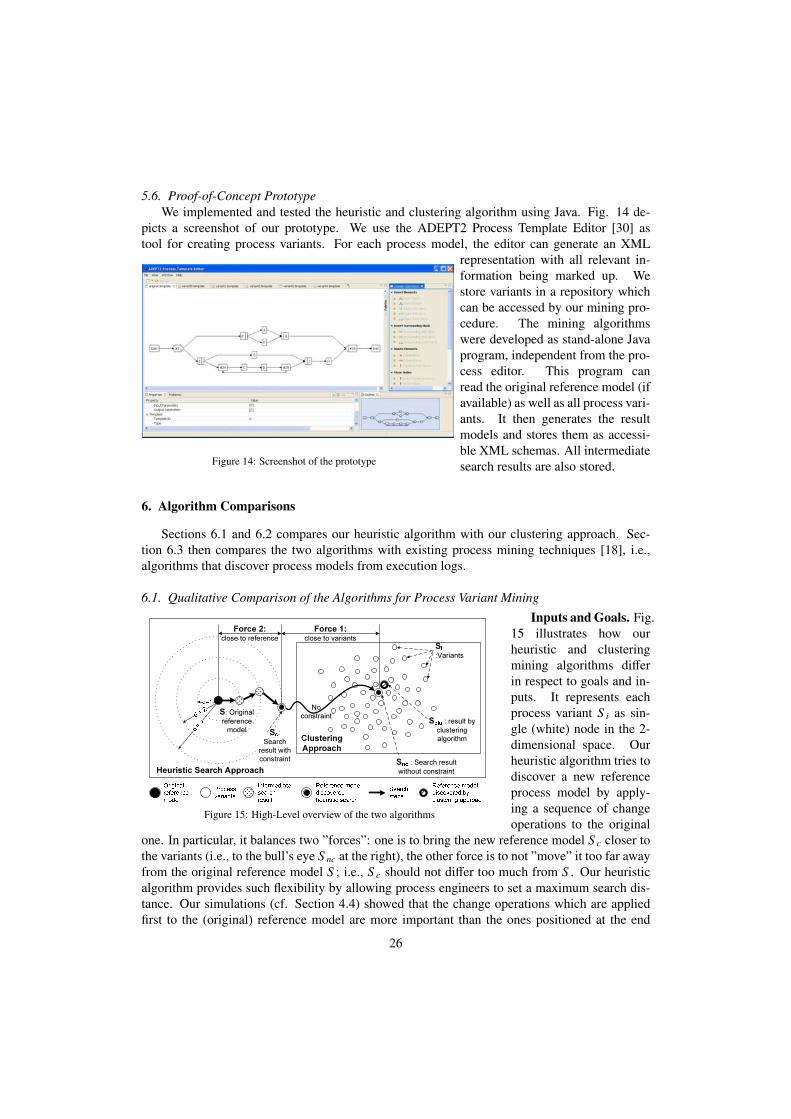
5.6. Proof-of-Concept PrototypeWe implemented and tested the heuristic and clustering algorithm using Java. Fig. 14 de-

picts a screenshot of our prototype. We use the ADEPT2 Process Template Editor [30] astool for creating process variants. For each process model, the editor can generate an XML

Figure 14: Screenshot of the prototype

representation with all relevant in-formation being marked up. Westore variants in a repository whichcan be accessed by our mining pro-cedure. The mining algorithmswere developed as stand-alone Javaprogram, independent from the pro-cess editor. This program canread the original reference model (ifavailable) as well as all process vari-ants. It then generates the resultmodels and stores them as accessi-ble XML schemas. All intermediatesearch results are also stored.

6. Algorithm Comparisons

Sections 6.1 and 6.2 compares our heuristic algorithm with our clustering approach. Sec-tion 6.3 then compares the two algorithms with existing process mining techniques [18], i.e.,algorithms that discover process models from execution logs.

6.1. Qualitative Comparison of the Algorithms for Process Variant Mining

No constraint

Snc : Search result without constraint

Si:Variants

d=1d = 2d = 3 S: Original reference

model

Reference model discovered heuristic searchOriginal reference model Process variants Intermediate search result Search stepsSc:

Search result with constraint

Force 1:close to variants

Force 2:close to reference

Sclu : result by clustering algorithm Clustering

Approach

Heuristic Search Approach Reference model discovered by clustering approachFigure 15: High-Level overview of the two algorithms

Inputs and Goals. Fig.15 illustrates how ourheuristic and clusteringmining algorithms differin respect to goals and in-puts. It represents eachprocess variant S i as sin-gle (white) node in the 2-dimensional space. Ourheuristic algorithm tries todiscover a new referenceprocess model by apply-ing a sequence of changeoperations to the original

one. In particular, it balances two ”forces”: one is to bring the new reference model S c closer tothe variants (i.e., to the bull’s eye S nc at the right), the other force is to not ”move” it too far awayfrom the original reference model S ; i.e., S c should not differ too much from S . Our heuristicalgorithm provides such flexibility by allowing process engineers to set a maximum search dis-tance. Our simulations (cf. Section 4.4) showed that the change operations which are appliedfirst to the (original) reference model are more important than the ones positioned at the end

26

i.e., they reduce distance between reference model and variants to a larger extent. Consequently,when ignoring less relevant changes we do not influence overall distance reduction too much.

While the above scenario presumes knowledge of the original reference model, we should beable to cope with cases in which there exists only a variant collection, but the original referenceprocess model is unknown. In this scenario, the goal of our clustering approach is to discover the”center” of the variants, i.e., a reference process model with shortest average weighted distanceto them. In principle, we can also apply our heuristic algorithm to this scenario. We just need tostart with an ”empty” model S without setting any search limitation. However, since we do notneed to balance the two forces and to perform the important change operations at the beginning ofthe search, the clustering algorithm is expected to be faster and to provide additional informationon the search result (see Section 6.2).

Design Principles and Complexity. Our heuristic algorithm discovers a better referencemodel by applying a sequence of change operations to the original one. To enable quick decisionsfor a large search space (cf. Section 4.2), we use a fitness function to evaluate how well acandidate model fits to the variants. This fitness function only provides a global evaluation, butdoes not show how each part of the candidate model fits to the variants. On the contrary, theclustering algorithm discovers a reference process model by enlarging blocks. By evaluatingseparation and cohesion, we are able to determine how well each part of the discovered referencemodel fits to the variants; i.e., due to its different design the clustering algorithm returns moreinformation than the heuristic one. Complexity of the two algorithms differs as well. Despitepolynomial complexity for computing the fitness of a candidate model, enumerating all blocksin a candidate model has NP-hard complexity.12 On the contrary, our clustering algorithmhas polynomial complexity since computing separation and cohesion are both polynomial. Tobe more precise, if m is the number of activities and n the one of variants, complexity of theclustering algorithm corresponds to O(m2n + m3). This implies that the clustering algorithmcan quickly compute the reference process model even for a large variant collection, while theheuristic algorithm may take considerable longer.

Pros & Cons. Table 5 summarizes the differences between the two algorithms. Additionalattention should be paid to their pros & cons. Since the clustering algorithm has polynomialcomplexity, it runs significantly faster than the heuristic one. Using Separation and Cohesionwe obtain information on how each part of the discovered reference process model fits to thevariants. However, our clustering algorithm cannot control the discovery procedure or distin-guish important changes from less relevant ones as our heuristic algorithm does. Though for ourrunning example the clustering algorithm discovered the same process model (cf. Fig. 13) asour heuristic algorithm (cf. Fig. 11), in many other cases the model discovered by the cluster-ing algorithm was not as good as the one discovered by the heuristic algorithm (cf. Section 6.2for details). Reason is that the heuristic algorithm searches a significantly larger space whichcontains a large number of candidate process models.

6.2. Quantitative Comparison of the Algorithms for Process Variant MiningWe now compare the two algorithms quantitatively by analyzing how fast they run and how

good the discovered models are. We use the same data for this comparison as for the evaluation of

12Worst-case, complexity of this algorithm is 2n where n corresponds to the number of activities. This worst-casescenario will only occur if any combination of activities may form a block (like a process model for which all activitiesare ordered in parallel to each other). During our simulation, in most cases we were able to enumerate all blocks of aprocess model within milliseconds. This indicates rather good performance in practice.

27

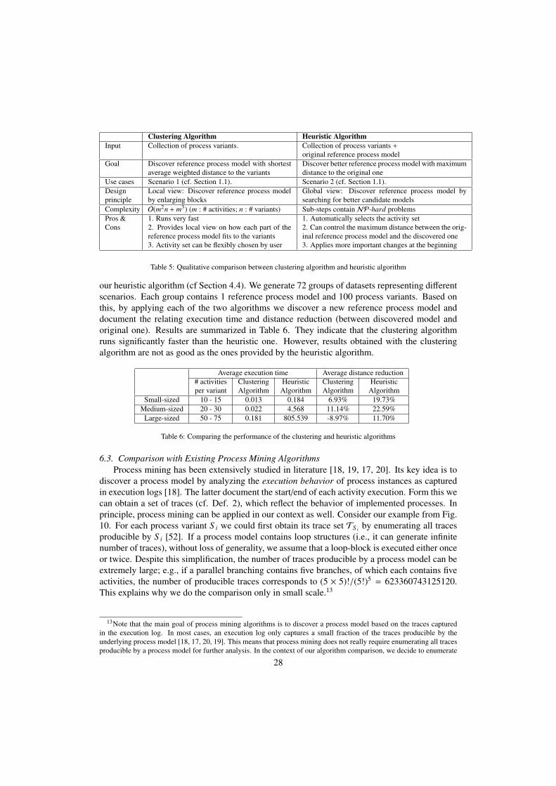
Clustering Algorithm Heuristic AlgorithmInput Collection of process variants. Collection of process variants +

original reference process modelGoal Discover reference process model with shortest

average weighted distance to the variantsDiscover better reference process model with maximumdistance to the original one

Use cases Scenario 1 (cf. Section 1.1). Scenario 2 (cf. Section 1.1).Designprinciple

Local view: Discover reference process modelby enlarging blocks

Global view: Discover reference process model bysearching for better candidate models

Complexity O(m2n + m3) (m : # activities; n : # variants) Sub-steps contain NP-hard problemsPros & 1. Runs very fast 1. Automatically selects the activity setCons 2. Provides local view on how each part of the

reference process model fits to the variants2. Can control the maximum distance between the orig-inal reference process model and the discovered one

3. Activity set can be flexibly chosen by user 3. Applies more important changes at the beginning

Table 5: Qualitative comparison between clustering algorithm and heuristic algorithm

our heuristic algorithm (cf Section 4.4). We generate 72 groups of datasets representing differentscenarios. Each group contains 1 reference process model and 100 process variants. Based onthis, by applying each of the two algorithms we discover a new reference process model anddocument the relating execution time and distance reduction (between discovered model andoriginal one). Results are summarized in Table 6. They indicate that the clustering algorithmruns significantly faster than the heuristic one. However, results obtained with the clusteringalgorithm are not as good as the ones provided by the heuristic algorithm.

Average execution time Average distance reduction# activities Clustering Heuristic Clustering Heuristicper variant Algorithm Algorithm Algorithm Algorithm

Small-sized 10 - 15 0.013 0.184 6.93% 19.73%Medium-sized 20 - 30 0.022 4.568 11.14% 22.59%

Large-sized 50 - 75 0.181 805.539 -8.97% 11.70%

Table 6: Comparing the performance of the clustering and heuristic algorithms

6.3. Comparison with Existing Process Mining AlgorithmsProcess mining has been extensively studied in literature [18, 19, 17, 20]. Its key idea is to

discover a process model by analyzing the execution behavior of process instances as capturedin execution logs [18]. The latter document the start/end of each activity execution. Form this wecan obtain a set of traces (cf. Def. 2), which reflect the behavior of implemented processes. Inprinciple, process mining can be applied in our context as well. Consider our example from Fig.10. For each process variant S i we could first obtain its trace set TS i by enumerating all tracesproducible by S i [52]. If a process model contains loop structures (i.e., it can generate infinitenumber of traces), without loss of generality, we assume that a loop-block is executed either onceor twice. Despite this simplification, the number of traces producible by a process model can beextremely large; e.g., if a parallel branching contains five branches, of which each contains fiveactivities, the number of producible traces corresponds to (5 × 5)!/(5!)5 = 623360743125120.This explains why we do the comparison only in small scale.13

13Note that the main goal of process mining algorithms is to discover a process model based on the traces capturedin the execution log. In most cases, an execution log only captures a small fraction of the traces producible by theunderlying process model [18, 17, 20, 19]. This means that process mining does not really require enumerating all tracesproducible by a process model for further analysis. In the context of our algorithm comparison, we decide to enumerate

28

The trace sets (cf. Def. 2) generated for the variants are merged into one trace set T takingthe weight of each variant into account. For example, as S 1 accounts for 25% of the variants, weensure that each trace producible by S 1 has the same number of instances and that the sum of allinstances producible by S 1 accounts for 25% of the instances in T as well. We consider T asexecution log since it fully covers the behavior of the given variant collection.

Since all activities contained in execution logs will be included in the process model discov-ered by process mining algorithms (like in our clustering algorithm), we introduce two additionaldatasets. The first one filters out all activities a j whose activity frequency g(a j) is lower than 0.2regarding the given variant collection (cf. Def. 12); i.e., in our example activity Z in S 5 and silentactivity τ (representing the loop in S 4) are ignored. For this extended data set, we determine traceset T0.2. In the second dataset, we filter out the activities with an activity frequency lower than0.6. Regarding our example, besides Z and τ we filter out activity Y in S 2, S 3, S 5, and S 6. Con-sequently, we obtain trace set T0.6 which contains all traces producible by the reduced variants.Note that T0.6 has the same activity set as the model discovered by our heuristic algorithm (cf.R4 in Fig. 11). The enumerated trace sets T , T0.2 and T0.6 are imported into the ProM frame-work, one of the most powerful tool for process mining and analysis [53]. In our comparison, weconsider alpha algorithm [18], heuristic miner [19], genetic mining [17], and multi-phase miner[20]. These are well-known algorithms for discovering process models from execution logs.14

6.3.1. Evaluation CriteriaOur algorithms focus on the structural perspective of process models, i.e., our goal is to con-

figure the variant models out of a reference model with minimal efforts (i.e., requiring a minimumnumber of high-level changes). On the contrary, traditional process mining focuses on processbehavior, i.e., the discovered process model should cover the behavior of the variant models (asreflected by their trace sets) [18, 17, 20, 19]. In the following, we compare our algorithms withexisting process mining algorithms from both a structural and a behavioral perspective.

Since most existing process mining algorithms discover Petri Nets or Event Process Chains(EPCs), we transform the process models discovered by the different algorithms into respectiverepresentations in order to enable their comparison (see [54, 52] for transformation techniques).Particularly, such model transformation enables us to reuse existing metrics [16, 24] and tools[53] for evaluating process models. We briefly describe the metrices we apply and refer to[16, 24, 53] for details. We first introduce three parameters to evaluate the structure of processmodels, namely average weighted distance, structural appropriateness, and # splits/joins in EPC.

1. Average weighted distance measures the efforts to configure the process variants out of

all traces producible by each variant for the following two reasons:1. In the context of our research, we do not assume the existence of an execution log. However, most process mining

evaluation criteria rely on traces, e.g., fitness, successful execution, proper completion, and behavioral appropriateness(cf. Section 6.3.1). Therefore, we adopt a general approach to first enumerate all traces and then to discover a processmodel. This way, we are able to compare all related mining algorithms based on the same approach.

2. Alternatively, we can randomly enumerate a collection of traces producible by a process model, and consider theserandom traces as execution log partially reflecting the behavior of the process model. However, we are not aware ofany technique which can enumerate a representative set of traces (but not all traces) to express the behavior of a processmodel. If we randomly select a fraction of traces, we cannot ensure a fair comparison since the results significantlydepend on the randomly selected trace set. Therefore, we decide to enumerate all traces producible by a process model.This way, we ensure that all possible behavior is considered, and results are not influenced by randomness.

14The enumerated trace sets T , T0.2 and T0.6 as well as the process models discovered by the different algorithms areavailable at http://wwwhome.cs.utwente.nl/~lic/Resources.html.

29

the discovered reference process model; the lower it is the easier the variants can be con-figured.

2. Structural appropriateness measures the complexity of a Petri Net by computing theratio between labeled transitions and nodes (transitions and places) [16]. The value rangeof this parameter is [0,1]; the higher it is, the simpler the Petri Net is.

3. # Splits/Joins in EPC measures the number of splits / joins of an EPC, and thus measuresits complexity [24]. The higher it is, the more choices end users need to make whenexecuting the EPC.

We additionally use three parameters to evaluate the behavior of the discovered process mod-els, namely behavior fitness, successful execution and proper completion.

1. Behavior fitness evaluates whether the discovered process model (represented as PetriNet) complies with the behavior as captured in the trace set [16]. One way to investigatebehavior fitness is to replay the traces on the Petri net. This is done in a non-blockingway, i.e., if there are missing tokens to fire a transition in the discovered model, they areartificially created and replay proceeds [16]. The value range of this parameter is [0,1].The higher behavior fitness is, the better the trace set will be covered by the model.

2. Successful execution measures the percentage of traces in the trace set that can be suc-cessfully executed by the discovered process model [16]. Its value range is [0,1]. Thehigher it is, the more traces can be re-produced based on the discovered model.

3. Proper completion measures the percentage of those traces that lead to proper completion[16]. When compared to ”successful execution” this parameter requires that the analyzedprocess model reaches an end state when replaying a trace. The value range of this param-eter is [0,1]. The higher it is, the more traces lead to proper completion.

Structure measurement Behavior measurement

Dataset Algorithms Average weig- Structural # Joins/ Behavior Successful Properhted distance appropriateness splits in EPC fitness execution completion

Heuristic Var. 2.4 0.481 6 0.876 0.353 0.353Clustering 4.75 0.468 8 0.737 0.120 0.120

Alpha 8.55 0.441 15 0.646 0 0T Heuristic 8.85 0.258 31 0.437 0.042 0

Genetic 6.6 0.341 19 0.811 0.342 0.009Multi-phase 2245 arcs and 515 transitions 19 In theory, all equals 1

Heuristic Var. 2.4 0.481 6 0.886 0.382 0.382Clustering 2.6 0.482 6 0.784 0.133 0.133

Alpha 6.9 0.466 12 0.706 0 0T0.2 Heuristic 8.2 0.274 12 0.789 0.268 0

Genetic 5.9 0.424 13 0.846 0.460 0.009Multi-phase 1534 arcs and 384 transitions 18 In theory, all equals 1

Heuristic Var. 2.4 0.481 6 0.851 0.327 0.337ClusteringAlpha 6.85 0.5 7 0.814 0.407 0

T0.6 Heuristic 7.85 0.462 10 0.736 0.407 0Genetic 3.2 0.325 13 0.886 0.394 0.278

Multi-phase 1266 arcs and 302 transitions 17 In theory, all equals 1

Table 7: Performance comparison with process mining algorithms

30

6.3.2. Evaluation ResultsEvaluation results are summarized in Table 7. To differentiate our heuristic algorithm from

heuristic miner known from process mining [19], we denote it as ”Heuristic var.” in Table 7.Without surprise, our heuristic and clustering algorithms discover a process model of simplestructure. Independent from the chosen dataset, the process models discovered by these algo-rithms have better scores for parameters relating to the structure of the discovered model; i.e.,they show lower average weighted distance, higher structural appropriateness, and lower numberof splits/joins in the corresponding EPC. Except multi-phase miner [20], none of the algorithmsdiscovered a process model with behavior fitness being 1. Note that multi-phase miner was de-signed in a way that it always discovers a process model with fitness 1. Despite the fact thatthe models discovered by multi-phase miner are very complex, they allow for more behavior notcovered by the variants [20, 16]; i.e., results are often overfitting.15 Consequently, we considerthe costs of multi-phase miner for reaching a behavior fitness of 1 as too high. When excludingmulti-phase miner, evaluation results show that even if we apply traditional process mining algo-rithms for discovering a process model that covers the behavior of the variants best, the resultingmodel might NOT be able to support all behavior captured by the variants. This indicates thenecessity for process configuration: i.e., it is not sufficient to maintain only one model coveringall behavior. Instead we must enable process configurations at both run- and build-time to obtaindifferent process variants supporting specific behaviors in different scenarios.

For the given dataset, behavior measurements of the process model discovered by our heuris-tic algorithm are good as well. Note that our heuristic algorithm discovered the same model (cf.R4 in Fig. 11) for T , T0.2 and T0.6. This model has highest behavior fitness for trace sets Tand T0.2, and only a few percent less than the genetic algorithm for T0.6. This was unexpectedbecause our heuristic algorithm is focusing on structure rather than on behavior. Though ouralgorithm focuses on the discovery of a reference model out of which the process variants can beeasily configured, this implies that behavior of the discovered model has not been sacrificed thatmuch. Since behavior fitness is not 1, however, we should apply process configurations to obtainsuited process variants supporting the execution of different process instances best.

7. Applying the Algorithms to a Practical Case

We applied our algorithms in a cast study in order to evaluate their practical benefits.Context. We conducted the case study in a large automotive company in which we analyzed

the variants of its product change management process. Basically, this process comprises severalmajor phases like specification of a change request, handling of this change request, change im-plementation, and roll-out. In the following we only consider the top-level process and commenton sub-processes later on. Usually, the change management process starts with the initiationof a Change Request (CR), which must then be detailed and assessed by different teams (e.g.,from engineering and production planning). The gathered comments then have to be aggregatedand approved by the CR board. In case of positive approval, change implementation starts, e.g.,detailing the planning and triggering the re-engineering of parts affected by the change.

15In principle, it is possible to measure overfitting using behavioral appropriateness [16]. However, due to the com-plexity of the discovered models, the conformance checker of ProM cannot measure some of the models (besides Multi-phase miner) in a reasonable time (e.g., within a couple of days). Therefore we did not include it in our comparison.

31

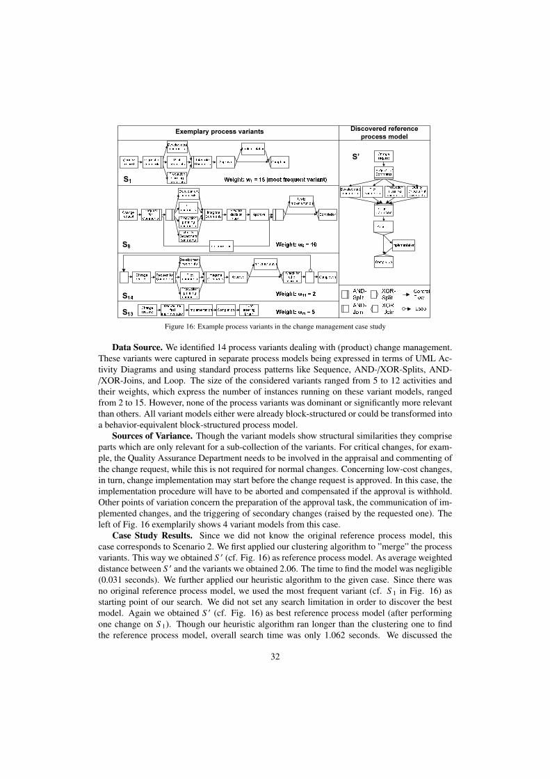
Change request Development commentsPilot commentsProduction planning comments Integrate Comments Request for Comments Approve CompletionImplementationChange request Development commentsPilot commentsProduction planning comments Integrate Comments Request for Comments CompletionUndo implementationQuality Department comments Implementation

Prepare decision paper ApproveExemplary process variants Discovered reference

process model

XOR-SplitXOR-Join Control FlowLoopAND-SplitAND-JoinChange request Development commentsPilot commentsProduction planning comments Integrate Comments Request for Comments Approve Check for other changesImplementation Completion

Change request

CompletionimplementationApproveDevelopment comments Pilot comments Production planning comments Quality Department commentsIntegrate Comments

Request for CommentsS1 Weight: w1 = 15 (most frequent variant)S8 Weight: w8 = 10S14 Weight: w14 = 2S13 Weight: wm = 5Change request Request for fast implementation Implementation Completion Inform steering board

S’

Figure 16: Example process variants in the change management case study

Data Source. We identified 14 process variants dealing with (product) change management.These variants were captured in separate process models being expressed in terms of UML Ac-tivity Diagrams and using standard process patterns like Sequence, AND-/XOR-Splits, AND-/XOR-Joins, and Loop. The size of the considered variants ranged from 5 to 12 activities andtheir weights, which express the number of instances running on these variant models, rangedfrom 2 to 15. However, none of the process variants was dominant or significantly more relevantthan others. All variant models either were already block-structured or could be transformed intoa behavior-equivalent block-structured process model.

Sources of Variance. Though the variant models show structural similarities they compriseparts which are only relevant for a sub-collection of the variants. For critical changes, for exam-ple, the Quality Assurance Department needs to be involved in the appraisal and commenting ofthe change request, while this is not required for normal changes. Concerning low-cost changes,in turn, change implementation may start before the change request is approved. In this case, theimplementation procedure will have to be aborted and compensated if the approval is withhold.Other points of variation concern the preparation of the approval task, the communication of im-plemented changes, and the triggering of secondary changes (raised by the requested one). Theleft of Fig. 16 exemplarily shows 4 variant models from this case.

Case Study Results. Since we did not know the original reference process model, thiscase corresponds to Scenario 2. We first applied our clustering algorithm to ”merge” the processvariants. This way we obtained S ′ (cf. Fig. 16) as reference process model. As average weighteddistance between S ′ and the variants we obtained 2.06. The time to find the model was negligible(0.031 seconds). We further applied our heuristic algorithm to the given case. Since there wasno original reference process model, we used the most frequent variant (cf. S 1 in Fig. 16) asstarting point of our search. We did not set any search limitation in order to discover the bestmodel. Again we obtained S ′ (cf. Fig. 16) as best reference process model (after performingone change on S 1). Though our heuristic algorithm ran longer than the clustering one to findthe reference process model, overall search time was only 1.062 seconds. We discussed the

32

discovered reference model with process engineers from the company who confirmed that itconstitutes a good choice for the top level change management process.

Based on the discovered reference process model, we can apply advanced techniques to con-figure it into the different process variants in an effective and manageable way. In the automotivecompany, in which we conducted the case study, the Provop research project was launched inwhich advanced concepts for managing and configuring process variants have been developed[10]. In Provop a particular process variant can be configured out of a given reference processmodel by domain experts by applying a set of high-level, pre-specified changes.

The presented mining algorithms can significantly speed up the design of such referenceprocess model. More precisely, respective reference models can be automatically discovered forany collection of block-structured process variants. When further applying our mining algorithmsto sub-processes relating to the different phases of the change management process (e.g., changeimplementation) and their variants we obtained good results as well.

Discussion. The case constitutes one of many process scenarios we encountered and ana-lyzed in the automotive domain. Interestingly, for almost all of them we were able to identifylarge collections of similar process variants, each of them being valid in a particular applicationcontext. Regarding the presented case, process owners liked the discovered reference processmodel and considered it as being intuitive. Based on this result, they asked us to apply ourmining approach to the more specific phases of the change management process as well, whichresulted in well accepted reference models for its sub-processes as well. We also studied othersources of data. Regarding release management for electric/ electronic components in a car, forexample, we identified more than 20 process variants depending on the product series, involvedsuppliers, or considered development phases. Another complex scenario we considered was theproduct creation process, for which dozens of variants exist. Thereby, each variant is assignedto a particular product type (e.g., car, truck, or bus) with different organizational responsibili-ties and strategic goals, or varying in some other aspects. Regarding the latter case, however,we encountered additional problems concerning the inconsistent labeling of activities, the use ofdifferent process granularities, and the heterogeneity of the used modeling formalisms. This alsoshows that our algorithms need to be integrated in a larger process repository framework, whichadditionally provides support for model configuration, refactoring, and management [15, 10].

Case studies in other domains. The practical benefit of our algorithms became evident inthe context of another case study we conducted in a clinical centre. We analyzed more than 90process variants for handling medical orders (e.g., X-ray inspections, lab tests). By applying ouralgorithms to these 90 variants we obtained a reference model that was significantly closer to thevariants than the old reference model. The discovered reference process model was adopted bythe clinical centre [55].

8. Related Work

Though algorithms applying heuristic search and clustering techniques have been widelyused in data mining [47], artificial intelligence [46], and machine learning [48], only few ap-proaches apply heuristics or clustering techniques in the context of process variant management.In particular, only few solutions exist for learning from the adaptations that were applied whenconfiguring a collection of process variants out of a reference process model.

Structural process changes at runtime and approaches for flexible process configuration havebeen intensively discussed [11, 4]. A comprehensive analysis of theoretical and practical issuesrelated to (dynamic) process changes has been provided in the ADEPT2 change framework [8].

33

Further, there exist approaches for dynamically changing the structure of Petri nets [40]. Basedon such frameworks, the AristaFlow BPM suite [30] and tools for configurable process models[56] emerged. [57, 58] additionally present repository services for storing, managing, and query-ing large collections of process variants. Graph-based search techniques are used for retrievingvariants that are similar to a process fragment specified by the user. Obviously, this requiresprofound knowledge about the structure of stored processes. Apart from this, no techniques foranalyzing the different variants and for learning from their specific customizations are provided.

ProCycle enables change reuse at the process instance level to effectively deal with recur-rent problem situations [11]. ProCycle applies case-based reasoning techniques to allow for thesemantic annotation as well as the retrieval of process changes. Respective process adaptationscan be reused in similar problem context later when configuring other process instances. If thereuse of a particular change exceeds a certain threshold, it becomes a candidate for adapting theprocess model at type level. Though the basic goal of ProCycle is similar to our approach, itstechniques are much simpler and do not consider change variation.

A process model can be represented as graph structure which enables different kinds of graph-based analyses [59, 47, 60, 61]. Informally, a graph consists of set of nodes, which can be con-nected using (directed) edges. Regarding graph representations there exist only few techniqueswhich foster learning from process variants by mining recorded change primitives (e.g., to addor delete control edges). [59] measures process model similarity based on change primitives andsuggests mining techniques using this measure. Similar techniques exist in the field of associ-ation rule mining [47], frequent sub-graph mining [60] and graph pattern discovery [61]; herecommon edges between different nodes are discovered to construct a common sub-graph froma set of graphs. We refer to [62] for a survey on graph mining topics and algorithms. However,graph-based approaches do not consider important features of a process meta model; e.g., theyare unable to deal with silent activities, cannot differentiate between AND- and XOR-branchingsor Loops, and cannot guarantee the soundness of the discovered process model.

Considering Configurable Workflow Models [56], all process variants are merged into onereference model based on inheritance rules known from Petri Nets [40]. Though techniques likequestionnaire-based configuration contribute to make the right configuration decisions [63], theresulting model turns out to be complex and often contains numerous decision points (see thecase reported in [64]). This approach even becomes more difficult when dealing with a largecollection of process variants not being equally important. In this case, an extremely large orcomplex process model results which contains too many decision points and cannot differentiatebetween important variants and trivial ones. In fields like healthcare, such complex models arenot preferred due to the resulting configuration efforts [65, 2].

To mine high-level change operations, [14] presents an approach based on process miningtechniques, i.e., the input consists of a change log and process mining algorithms are appliedto discover the execution sequences of the changes (i.e., the change meta process). However,this approach simply considers each change as individual operation such that the result is morelike a visualization of changes rather than their mining. [66] introduces a technique to rankactivities based on their potential involvement in process configurations. However, it cannotprovide suggestions on how to involve these activities in model changes to improve the referenceprocess model.

34

9. Summary and Outlook

We presented challenges, scenarios and algorithms for mining a collection of process vari-ants. In particular, we introduced, evaluated and compared two algorithms for discovering areference process model out of a collection of block-structured process variants. Adopting thediscovered model as new reference process model makes future process configuration easier,since less efforts for configuring the variants will be required. Our heuristic algorithm can takethe original reference model into account such that users can control to what degree the discov-ered model differs from the original one. This way, we can avoid Spaghetti-like process models,and also control how many changes we want to perform. Through a simulation of several thou-sands process models we learned that the heuristic algorithm applies the important changes atthe beginning of the search and is able to scale up. The clustering algorithm, in turn, does notpresume any knowledge about the original reference process model the process variants wereconfigured from. By only looking at the variant collection, it can quickly discover a referenceprocess model in polynomial time and provide additional information on how well each part ofthe discovered reference model fits to the variants. We successfully applied the two algorithmsto practical cases. We further compared them with existing process mining algorithms. Resultsindicate good performance of our algorithms in both structure and behavior aspect. However, itwould be useful to integrate them with existing process mining algorithms such that we can takeboth the structural and the behavioral perspective into account in order to cover more generalcases [18]. As we learned, data-flow also constitutes an important part of process configurations.Therefore, we want to additionally consider this perspective in future research.

Acknowledgment: This work was done in the MinAdept project, which has been supportedby the Netherlands Organization for Scientific Research under contract number 612.066.512.

References

[1] B. Mutschler, M. Reichert, and J. Bumiller. Unleashing the effectiveness of process-oriented information systems:Problem analysis, critical success factors and implications. IEEE Trans. Sys. Man. & Cyb., 38(3):280–291, 2008.

[2] R. Lenz and M. Reichert. IT support for healthcare processes - premises, challenges, perspectives. Data & Knowl-edge Engineering, 61(1):39–58, 2007.

[3] T.H. Davenport. Mission Critical - Realizing the Promise of Enterprise Systems. Harvard Business School, 2000.[4] B. Weber, M. Reichert, and S. Rinderle-Ma. Change patterns and change support features - enhancing flexibility in

process-aware information systems. Data and Knowledge Engineering, 66(3):438–466, 2008.[5] B. Weber, S. Sadiq, and M. Reichert. Beyond rigidity - dynamic process lifecycle support: A survey on dynamic

changes in process-aware information systems. Computer Science - R&D, 23(2):47–65, 2009.[6] A. Hallerbach, T. Bauer, and M. Reichert. Managing process variants in the process lifecycle. In ICEIS ’08, pages

154–161. Springer, 2008.[7] M. Rosemann and W.M.P. van der Aalst. A configurable reference modelling language. Information Systems,

32(1):1–23, 2007.[8] M. Reichert and P. Dadam. ADEPTflex - supporting dynamic changes of workflows without losing control. Journal

of Intelligent Information Systems, 10(2):93–129, 1998.[9] M. Rosenmann. Potential pitfalls of process modeling: part B. BPM Journal, 12(3):127–136, 2006.

[10] A. Hallerbach, T. Bauer, and M. Reichert. Capturing variability in business process models: the Provop approach.Journal of Software Maintenance and Evolution, 22(6-7):519–546, 2010.

[11] B. Weber, M. Reichert, W. Wild, and S. Rinderle-Ma. Providing integrated life cycle support in process-awareinformation systems. Int’l Journal of Cooperative Information Systems, 19(1):115–165, 2009.

[12] B. Kiepuszewski, A.H.M. ter Hofstede, and C. Bussler. On structured workflow modelling. In CAiSE’00, pages431–445. LNCS 1789, Springer, 2000.

[13] R.M. Dijkman, M. Dumas, L. Garcia-Banuelos, and R. Kaarik. Aligning business process models. In EDOC’09,pages 45–53, 2009.

[14] C.W. Gunther, S. Rinderle-Ma, M. Reichert, W.M.P. van der Aalst, and J. Recker. Using process mining to learnfrom process changes in evolutionary systems. Int’l J. of Business Process Int. and Mgmt, 3(1):61–78, 2008.

35

[15] B. Weber, M. Reichert, J. Mendling, and H.A. Reijers. Refactoring large process model repositories. Computers inIndustry, page accepted for publication.

[16] A. Rozinat and W.M.P. van der Aalst. Conformance checking of processes based on monitoring real behavior.Information Systems, 33(1):64–95, 2008.

[17] A.K. Alves de Medeiros. Genetic Process Mining. PhD thesis, Eindhoven University of Technology, NL, 2006.[18] W.M.P van der Aalst, T. Weijters, and L. Maruster. Workflow mining: Discovering process models from event

logs. IEEE Trans. on Knowl. and Data Eng., 16(9):1128–1142, 2004.[19] A.J.M.M. Weijters and W.M.P. van der Aalst. Rediscovering workflow models from event-based data using little

thumb. Integr. Comput.-Aided Eng., 10(2):151–162, 2003.[20] B.F. van Dongen and W.M.P. van der Aalst. Multi-phase process mining: Building instance graphs. In ER’04,

pages 362–376. LNCS 3288, Springer, 2004.[21] C. Li, M. Reichert, and A. Wombacher. Discovering reference models by mining process variants using a heuristic

approach. In BPM’09, LNCS 5701, pages 344–362. Springer, 2009.[22] W.M.P. van der Aalst, A.H.M. ter Hofstede, B. Kiepuszewski, and A.P. Barros. Workflow patterns. Distributed and

Parallel Databases, 14(1):5–51, 2003.[23] M. zur Muehlen and J. Recker. How much language is enough? Theoretical and practical use of the business

process modeling notation. In CAiSE’08, pages 465–479. LNCS 5074, Springer, 2008.[24] J. Mendling. Metrics for Process Models: Empirical Foundations of Verification, Error Prediction and Guidelines

for Correctness, volume 6 of LNBIP. Springer, 2008.[25] BPEL. http://docs.oasis-open.org/wsbpel/2.0/wsbpel-v2.0.pdf.[26] W.M.P. van der Aalst and K. van Hee. Workflow Management: Models, Methods, and Systems. MIT Press, 2002.[27] J. Mendling, B.F. van Dongen, and W.M.P. van der Aalst. Getting rid of OR-joins and multiple start events in

business process models. Enterprise Information Systems, 2(4):403–419, 2008.[28] C. Li, M. Reichert, and A. Wombacher. On measuring process model similarity based on high-level change opera-

tions. In ER ’08, pages 248–262. Springer LNCS 5231, 2008.[29] M. Reichert. Dynamische Ablaufanderungen in Workflow-Management-Systemen. PhD thesis, Ulm University,

Germany, 2000.[30] M. Reichert, S. Rinderle, U. Kreher, and P. Dadam. Adaptive process management with ADEPT2. In ICDE ’05,

pages 1113–1114. IEEE Computer Press, 2005.[31] J. Vanhatalo, H. Volzer, and J. Koehler. The refined process structure tree. Data & Knowledge Engineering,

68(9):793–818, 2009.[32] E.W. Dijkstra. Notes on structured programming. pages 1–82, 1972.[33] P. Dadam and M. Reichert. The ADEPT project: A decade of research and development for robust and flexible

process support - challenges and achievements. Computer Science - R & D, 23(2):81–97, 2009.[34] M. Minor, A. Tartakovski, D. Schmalen, and R. Bergmann. Agile workflow technology and case-based change

reuse for long-term processes. International Journal of Intelligent Information Technologies, 4(1):80–98, 2008.[35] H.A. Reijers and J. Mendling. Modularity in process models: Review and effects. In BPM’08, pages 20–35. LNCS

5240, Springer, 2008.[36] J. Mendling, H.A. Reijers, and W.M.P. van der Aalst. Seven process modeling guidelines (7pmg). Information &

Software Technology, 52(2):127–136, 2010.[37] C. Combi and M. Gambini. Flaws in the flow: The weakness of unstructured business process modeling languages

dealing with data. In OTM Conferences (1), pages 42–59. LNCS 5870, Springer, 2009.[38] L. Thom, M. Reichert, and C. Iochpe. Activity patterns in process-aware information systems: Basic concepts and

empirical evidence. Int. J. of Business Process Int. and Mgmt, 4(2):93–110, 2009.[39] S. Rinderle. Schema Evolution in Process Management Systems. PhD thesis, Ulm University, Germany, 2004.[40] W.M.P. van der Aalst and T. Basten. Inheritance of workflows: an approach to tackling problems related to change.

Theor. Comput. Sci., 270(1-2):125–203, 2002.[41] S. Rinderle-Ma, M. Reichert, and B. Weber. On the formal semantics of change patterns in process-aware infor-

mation systems. In ER’08, LNCS 5231, pages 279–293, 2008.[42] A. Lanz, U. Kreher, M. Reichert, and P. Dadam. Enabling process support for advanced applications with the

AristaFlow BPM Suite. In BPM’10 Demonstration Track. Vol. 615 CEUR-WS.org, 2010.[43] A.V. Aho, M.S. Lam, R. Sethi, and J.D. Ullman. Compilers: Principles, Techniques, and Tools (2nd Edition).

Addison Wesley, 2006.[44] D. Harel and R.E. Tarjan. Fast algorithms for finding nearest common ancestors. SIAM Journal on Computing,

13(2):338–355, 1984.[45] C. Li, M. Reichert, and A. Wombacher. Representing block-structured process models as order matrices: Basic

concepts, formal properties, algorithms. Technical Report TR-CTIT-09-47, University of Twente, NL, 2009.[46] G. F. Luger. Artificial Intelligence: Structures and Strategies for Complex Problem Solving. Pearson, 2005.[47] P.N. Tan, M. Steinbach, and V. Kumar. Introduction to Data Mining. Addison-Wesley, 2005.

36

[48] J. Ross Quinlan. C4.5: programs for machine learning. Morgan Kaufmann Publishers Inc., USA, 1993.[49] A.M. Law. Simulation modeling and analysis. McGraw-Hill Higher Education, 2006.[50] C. Li, M. Reichert, and A. Wombacher. A heuristic approach for discovering reference models by mining process

model variants. Technical Report TR-CTIT-09-08, University of Twente, The Netherlands, March 2009.[51] D.J. Sheskin. Handbook of Parametric and Nonparametric Statistical Procedures. CRC Press, 2004.[52] A. Wombacher, P. Fankhauser, and E. Neuhold. Transforming bpel into annotated deterministic finite state automata

for service discovery. Web Services, IEEE International Conference on, 0:316, 2004.[53] B.F. van Dongen, A.K.A. de Medeiros, H.M.W. Verbeek, A.J.M.M. Weijters, and W.M.P. van der Aalst. The ProM

framework: A new era in process mining tool support. In ICATPN, pages 444–454. LNCS 3536, 2005.[54] J. Dehnert and R. Rittgen. Relaxed soundness of business processes. In CAiSE ’01, pages 157–170. LNCS 2068,

Springer, 2001.[55] C. Li, M. Reichert, and A. Wombacher. The MinAdept clustering approach for discovering reference process

models out of process variants. Int’l J. of Cooperative Information Systems, 19(3 & 4):159–203, 2010.[56] F. Gottschalk, W.M.P. van der Aalst, M.H. Jansen-Vullers, and M. La Rosa. Configurable workflow models. Int. J.

Cooperative Inf. Syst., 17(2):177–221, 2008.[57] R. Lu and S.W. Sadiq. Managing process variants as an information resource. In BPM’06, pages 426–431, 2006.[58] R. Lu and S. W. Sadiq. On the discovery of preferred work practice through business process variants. In ER’07,

pages 165–180. Springer, 2007.[59] J. Bae, L. Liu, J. Caverlee, L.J. Zhang, and H. Bae. Development of distance measures for process mining, discovery

and integration. Int. J. Web Service Res., 4(4):1–17, 2007.[60] M. Kuramochi and G. Karypis. Frequent subgraph discovery. In ICDM’01, pages 313–320. IEEE, 2001.[61] X. Yan and J. Han. gspan: Graph-based substructure pattern mining. In ICDM’02, pages 721–724. IEEE Computer

Society, 2002.[62] D. Chakrabarti and C. Faloutsos. Graph mining: Laws, generators, and algorithms. ACM Computing Surveys,

38(1):2, 2006.[63] M. la Rosa, W.M.P. van der Aalst, M. Dumas, and A.H.M. ter Hofstede. Questionnaire-based variability modeling

for system configuration. Software and System Modeling, 8(2):251–274, 2009.[64] F. Gottschalk, T. A. C. Wagemakers, M. H. Jansen-Vullers, W.M.P. van der Aalst, and M. La Rosa. Configurable

process models: Experiences from a municipality case study. In CAiSE’09, pages 486–500, 2009.[65] J.S. Ash, M. Berg, and E. Coiera. Some unintended consequences of information technology in health care: the

nature of patient care information system-related errors. J. Am. Med. Inf. Ass., 11(2):104–112, 2004.[66] C. Li, M. Reichert, and A. Wombacher. What are the problem makers: Ranking activities according to their

relevance for process changes. In ICWS’09, pages 51–58. IEEE, 2009.

Appendix A. Properties of Block-structured Process Model

Let S = (A, E, AT, ET, l) be a block-structured process model (cf. Def. 1). Then: S has thefollowing structural properties:

1. S has a unique start node; i.e.; ∃!s ∈ A : ∀(a1, a2) ∈ E : a2 , s.s is the only node with AT (s) = StartFlow.

2. S has a unique end node; i.e.; ∃!e ∈ A : ∀(a1, a2) ∈ E : a1 , e.e is the only node with AT (e) = EndFlow.

3. Let Atypes be defined as Atypes := {a ∈ A|AT (a) ∈ types}, Then:

• Each non-split node (excl. the end node) has exactly one outgoing precedence edge:∀a ∈ A \ AAndS plit

⋃XorS plit

⋃EndFlow :

∃!e = (a1, a2) ∈ E with a1 = a ∧ ET (e) = Precedence.• Each non-join node (excl. the start node) has exactly one incoming precedence edge:∀a ∈ A \ AAndJoin

⋃XorJoin

⋃S tartFlow :

∃!e = (a1, a2) ∈ E with a2 = a ∧ ET (e) = Precedence.• Any loop edge links a StartLoop node with an EndLoop node:∀e = (a1, a2) ∈ E with ET (e) = Loop,⇒ AT (a1) = StartLoop ∧ AT (a2) = EndLoop.

37

4. S is block-structured –i.e., the following properties hold:

• Let S plits, Joins ⊂ A be defined as follows:S plits := AAndS plit

⋃XorS plit, Joins := AAndJoin

⋃XorJoin.

Then: There exists a mapping join : S plits→ Joins with:– s ∈ S plits,⇒ s ≺ join(s).– join is a bijective mapping, i.e., join(s1) = join(s2) for s1, s2 ∈ S plits,⇒

s1 = s2 ∧ ∀ j ∈ Joins : ∃s ∈ S plits : join(s) = j.– Let s ∈ S plits:

The subgraph induced by {s, join(s)} ⋃ {a ∈ A|s ≺ a ∧ a ≺ join(s)} is a SESE,i.e., a subgraph with single entry and single exit node.

– s ∈ S plits ∧ AT (s) = AndSplit(XorSplit),⇒ AT ( join(s)) = AndJoin(XorJoin).

• There exists a bijective mapping loop : AS tartLoop → AEndLoop with:– ls ∈ AS tartLoop,⇒ loop(ls) ≺ ls– ls ∈ AS tartLoop,⇒ The subgraph induced by{ls, loop(ls)}⋃ {a ∈ A|loop(ls) ≺ a ∧ a ≺ ls} is a SESE.

• Blocks must not overlap, i.e., their nesting must be regular. Formally:Bstarts ≡ S plits

⋃AEndLoop; Bends ≡ Joins

⋃AS tartLoop.

Further, Let block be a mapping,block : Bstarts → Bends with block(s) = join(s) ifs ∈ S plits and block(s) = loop−1(s) if s ∈ AEndLoop. Then: s1, s2 ∈ Bstarts withs1 ≺ s2 ≺ block(s1),⇒ block(s2) ≺ block(s1).

Appendix B. Proof of Theorem 1

Theorem 1 (cf. Section 3.1.3) states that we obtain a unique order matrix A for a processstructure tree T = (N,C,CT, E, l), i.e., for two nodes ai, a j ∈ N, NCA(ai, a j) exists and is unique.The proof consists of 3 steps:

1. Based on the properties of process structure tree (cf. Theorem 2), we first prove that theindegree of any element in a process structure tree is less or equal to 1 (cf. Theorem 3).

2. We show that for any two connected nodes in a process structure tree, there exists exactlyone path linking them (cf. Lemma 1).

3. Finally, we prove that for any two different nodes in a process structure tree, their nearestcommon ancestor exists and is unique (cf. Theorem 4).

We first discuss an important property of any process structure tree T = (N,C,CT, E, l),namely that a subtree of T does not overlap with another different subtree of T . This property isdescribed by Theorem 2. For a proof of Theorem 2, we refer to [31].

Theorem 2. Let T = (N,C,CT, E, l) be a process structure tree and let T ′ = (N′,C′,CT ′, E′, l′)and T ′′ = (N′′,C′′,CT ′, E′′, l′′) be two different subtrees of T . Then: T ′ does not overlap withT ′′; i.e., either T ′ is a subtree of T ′′, or T ′′ is a subtree of T ′, or the following property holds((N′

⋂N′′ = ∅) ∧ (C′

⋂C′′ = ∅) ∧ (E′

⋂E′′ = ∅)).

Based on Theorem 2, we can obtain Theorem 3.

Theorem 3. The indegree in(e) of any element e ∈ N⋃

C in a process structure tree T =

(N,C,CT, E, l) is less or equal 1.38

Proof. Assume there exists an element e ∈ N⋃

C which has more than one predecessor; i.e.,∃n1, n2, . . . , ni ∈ N

⋃C : (n1, e), (n2, e), . . . , (ni, e) ∈ E and nx , ny for x, y ∈ {1, . . . , i}. Let

T (nx) and T (ny) be two subtrees that result when using nx and ny as their root elements (withx, y ∈ {1, . . . , i}, x , y) (cf. Section 3.1.1). Then, T (nx) and T (ny) contain element e since(nx, e) ∈ E and (ny, e) ∈ E. However, since nx , ny holds, T (nx) cannot be a subtree of T (ny), andvice versa. Therefore, T (nx) and T (ny) overlap, which contradicts to the property described inTheorem 2. Consequently, any element e ∈ N

⋃C maximally has one predecessor, i.e., in(e) ≤ 1;

in(e) = 0 holds if e is the root of T .

Based on Theorem 3, we can obtain Lemma 1.

Lemma 1. For two connected nodes a, b ∈ N⋃

C in a process structure tree T = (N,C,CT, E, l),there exists exactly one path connecting a with b.

Proof. Let a, b ∈ N⋃

C be two elements of T . Assume that a and b are connected with a ≺ b.Then there exists a sequence < n0, n1, . . . , ni > with n0, . . . , ni ∈ N

⋃C, n0 = a, ni = b and

(nk−1, nk) ∈ E for k ∈ {1, . . . , i}. According to Theorem 3, in(nk) ≤ 1 holds ⇒ The node whichdirectly precedes nk is unique and corresponds to nk−1. Since this applies to all k ∈ {1, . . . , i}, thepath < n0, . . . , ni > is unique.

Finally, Theorem 4 describes the existence and uniqueness of the nearest common ancestorfor any two different nodes in a process structure tree.

Theorem 4. Taking two different nodes a, b ∈ N in a process structure tree T = (N,C,CT, E, l),their nearest common ancestor NCA(a, b) exists and is unique.

Proof. Let a, b ∈ N be two different nodes and let further c ∈ C be the nearest common ancestorof a and b. Since a and b are two different nodes, T contains at minimum two nodes and oneconnector. Consequently, there must be a root connector r ∈ E with r ≺ a and r ≺ b, since nodesconstitute the leaves in the tree and cannot be a predecessor of any other tree element.

• Existence of c. Since each process structure tree has a unique root r, we obtain r ≺ a andr ≺ b. According to Lemma 1, we can find two unique paths < n0, n1, . . . , ni > with n0 = rand ni = a, and < n′0, n

′1, . . . , n

′j > with n′0 = r and n′j = b respectively. Let min(i, j) denote

the minimum of i and j. Since r = n0 = n′0, there must be a k with 0 ≤ k ≤ min(i, j) suchthat n0 = n′0, n1 = n′1, . . ., nk = n′k. According to Def. 8 we obtain nk as NCA(a, b).

• Uniqueness of c. Assume there is another connector c′ , c with c′ ∈ C, which is a nearestcommon ancestor of a and b. According to Def. 8 we obtain c ⊀ c′ and c′ ⊀ c. Let r bethe unique root of process structure tree T . Then we obtain r ≺ c and r ≺ c′. Since c′ iscommon ancestor of a and b, we obtain c′ ≺ a and c′ ≺ b. Consequently, there are twodifferent paths from r to a: < r, . . . , c, . . . , a > and < r, . . . , c′, . . . , a >. This contradicts toLemma 1⇒ c′ cannot exist.

39

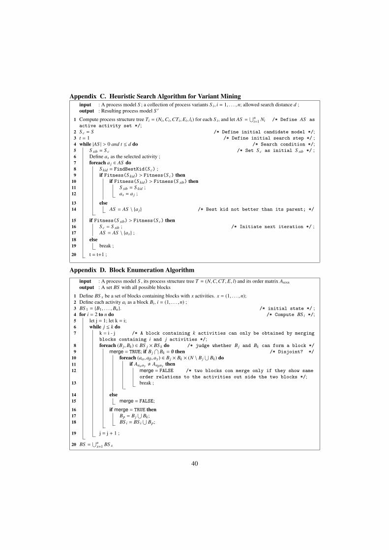
Appendix C. Heuristic Search Algorithm for Variant Mininginput : A process model S ; a collection of process variants S i, i = 1, . . . , n; allowed search distance d ;output : Resulting process model S ′

Compute process structure tree Ti = (Ni,Ci,CTi, Ei, li) for each S i, and let AS =⋃n

i=1 Ni /* Define AS as1active activity set */;S c = S /* Define initial candidate model */;2t = 1 /* Define initial search step */ ;3while |AS | > 0 and t ≤ d do /* Search condition */;4

S sib = S c /* Set S c as initial S sib */ ;5Define as as the selected activity ;6foreach a j ∈ AS do7

S kid = FindBestKid(S c) ;8if Fitness(S kid) > Fitness(S c) then9

if Fitness(S kid) > Fitness(S sib) then10S sib = S kid ;11as = a j ;12

else13AS = AS \ {a j} /* Best kid not better than its parent; */14

if Fitness(S sib) > Fitness(S c) then15S c = S sib ; /* Initiate next iteration */ ;16AS = AS \ {as} ;17

else18break ;19

t = t+1 ;20

Appendix D. Block Enumeration Algorithm

input : A process model S , its process structure tree T = (N,C,CT, E, l) and its order matrix An×noutput : A set BS with all possible blocks

Define BS x be a set of blocks containing blocks with x activities. x = (1, . . . , n);1Define each activity ai as a block Bi, i = (1, . . . , n) ;2BS 1 = {B1, . . . , Bn}. /* initial state */ ;3for i = 2 to n do /* Compute BS i */;4

let j = 1; let k = i;5while j ≤ k do6

k = i - j /* A block containing k activities can only be obtained by merging7blocks containing i and j activities */;foreach (B j, Bk) ∈ BS j × BS k do /* judge whether B j and Bk can form a block */8

merge = TRUE; if B j⋂

Bk = ∅ then /* Disjoint? */9foreach (aα, aβ, aγ) ∈ B j × Bk × (N \ B j

⋃Bk) do10

if Aaαaγ , Aaβaγ then11merge = FALSE /* two blocks con merge only if they show same12order relations to the activities out side the two blocks */;break ;13

else14merge = FALSE;15

if merge = TRUE then16Bp = B j

⋃Bk;17

BS i = BS i⋃

Bp;18

j = j + 1 ;19

BS =⋃n

x=1 BS x20

40