mining frequent patterns without candidate · pdf filemining frequent patterns without...

Data Mining and Knowledge Discovery, 8, 53–87, 2004c! 2004 Kluwer Academic Publishers. Manufactured in The Netherlands.

Mining Frequent Patterns without CandidateGeneration: A Frequent-Pattern TreeApproach!

JIAWEI HAN [email protected] of Illinois at Urbana-Champaign

JIAN PEI† [email protected] University of New York at Buffalo

YIWEN YIN [email protected] Fraser University

RUNYING MAO [email protected] Corporation

Editor: Heikki Mannila

Received May 21, 2000; Revised April 21, 2001

Abstract. Mining frequent patterns in transaction databases, time-series databases, and many other kinds ofdatabases has been studied popularly in data mining research. Most of the previous studies adopt an Apriori-likecandidate set generation-and-test approach. However, candidate set generation is still costly, especially when thereexist a large number of patterns and/or long patterns.

In this study, we propose a novel frequent-pattern tree (FP-tree) structure, which is an extended prefix-treestructure for storing compressed, crucial information about frequent patterns, and develop an efficient FP-tree-based mining method, FP-growth, for mining the complete set of frequent patterns by pattern fragment growth.Efficiency of mining is achieved with three techniques: (1) a large database is compressed into a condensed,smaller data structure, FP-tree which avoids costly, repeated database scans, (2) our FP-tree-based mining adoptsa pattern-fragment growth method to avoid the costly generation of a large number of candidate sets, and (3) apartitioning-based, divide-and-conquer method is used to decompose the mining task into a set of smaller tasks formining confined patterns in conditional databases, which dramatically reduces the search space. Our performancestudy shows that the FP-growth method is efficient and scalable for mining both long and short frequent patterns,and is about an order of magnitude faster than the Apriori algorithm and also faster than some recently reportednew frequent-pattern mining methods.

Keywords: frequent pattern mining, association mining, algorithm, performance improvements, data structure

!The work was done at Simon Fraser University, Canada, and it was supported in part by the Natural Sciencesand Engineering Research Council of Canada, and the Networks of Centres of Excellence of Canada.†To whom correspondence should be addressed.

54 HAN ET AL.

1. Introduction

Frequent-pattern mining plays an essential role in mining associations (Agrawal et al.,1993, 1996; Agrawal and Srikant, 1994; Mannila et al., 1994), correlations (Brin et al.,1997), causality (Silverstein et al., 1998), sequential patterns (Agrawal and Srikant, 1995),episodes (Mannila et al., 1997), multi-dimensional patterns (Lent et al., 1997; Kamberet al., 1997), max-patterns (Bayardo, 1998), partial periodicity (Han et al., 1999), emergingpatterns (Dong and Li, 1999), and many other important data mining tasks.

Most of the previous studies, such as Agrawal and Srikant (1994), Mannila et al. (1994),Agrawal et al. (1996), Savasere et al. (1995), Park et al. (1995), Lent et al. (1997), Sarawagiet al. (1998), Srikant et al. (1997), Ng et al. (1998) and Grahne et al. (2000), adopt anApriori-like approach, which is based on the anti-monotone Apriori heuristic (Agrawal andSrikant, 1994): if any length k pattern is not frequent in the database, its length (k + 1)super-pattern can never be frequent. The essential idea is to iteratively generate the set ofcandidate patterns of length (k +1) from the set of frequent-patterns of length k (for k " 1),and check their corresponding occurrence frequencies in the database.

The Apriori heuristic achieves good performance gained by (possibly significantly) re-ducing the size of candidate sets. However, in situations with a large number of frequentpatterns, long patterns, or quite low minimum support thresholds, an Apriori-like algorithmmay suffer from the following two nontrivial costs:

– It is costly to handle a huge number of candidate sets. For example, if there are 104

frequent 1-itemsets, the Apriori algorithm will need to generate more than 107 length-2candidates and accumulate and test their occurrence frequencies. Moreover, to discovera frequent pattern of size 100, such as {a1, . . . , a100}, it must generate 2100 # 2 $ 1030

candidates in total. This is the inherent cost of candidate generation, no matter whatimplementation technique is applied.

– It is tedious to repeatedly scan the database and check a large set of candidates by patternmatching, which is especially true for mining long patterns.

Can one develop a method that may avoid candidate generation-and-test and utilize somenovel data structures to reduce the cost in frequent-pattern mining? This is the motivationof this study.

In this paper, we develop and integrate the following three techniques in order to solvethis problem.

First, a novel, compact data structure, called frequent-pattern tree, or FP-tree in short,is constructed, which is an extended prefix-tree structure storing crucial, quantitative infor-mation about frequent patterns. To ensure that the tree structure is compact and informative,only frequent length-1 items will have nodes in the tree, and the tree nodes are arranged insuch a way that more frequently occurring nodes will have better chances of node sharingthan less frequently occurring ones. Our experiments show that such a tree is compact,and it is sometimes orders of magnitude smaller than the original database. Subsequentfrequent-pattern mining will only need to work on the FP-tree instead of the whole data set.

Second, an FP-tree-based pattern-fragment growth mining method is developed, whichstarts from a frequent length-1 pattern (as an initial suffix pattern), examines only its

MINING FREQUENT PATTERNS WITHOUT CANDIDATE GENERATION 55

conditional-pattern base (a “sub-database” which consists of the set of frequent items co-occurring with the suffix pattern), constructs its (conditional) FP-tree, and performs miningrecursively with such a tree. The pattern growth is achieved via concatenation of the suffixpattern with the new ones generated from a conditional FP-tree. Since the frequent itemsetin any transaction is always encoded in the corresponding path of the frequent-pattern trees,pattern growth ensures the completeness of the result. In this context, our method is notApriori-like restricted generation-and-test but restricted test only. The major operations ofmining are count accumulation and prefix path count adjustment, which are usually muchless costly than candidate generation and pattern matching operations performed in mostApriori-like algorithms.

Third, the search technique employed in mining is a partitioning-based, divide-and-conquer method rather than Apriori-like level-wise generation of the combinations of fre-quent itemsets. This dramatically reduces the size of conditional-pattern base generated atthe subsequent level of search as well as the size of its corresponding conditional FP-tree.Moreover, it transforms the problem of finding long frequent patterns to looking for shorterones and then concatenating the suffix. It employs the least frequent items as suffix, whichoffers good selectivity. All these techniques contribute to substantial reduction of searchcosts.

A performance study has been conducted to compare the performance of FP-growth withtwo representative frequent-pattern mining methods, Apriori (Agrawal and Srikant, 1994)and TreeProjection (Agarwal et al., 2001). Our study shows that FP-growth is about anorder of magnitude faster than Apriori, especially when the data set is dense (containingmany patterns) and/or when the frequent patterns are long; also, FP-growth outperformsthe TreeProjection algorithm. Moreover, our FP-tree-based mining method has been im-plemented in the DBMiner system and tested in large transaction databases in industrialapplications.

Although FP-growth was first proposed briefly in Han et al. (2000), this paper makesadditional progress as follows.

– The properties of FP-tree are thoroughly studied. Also, we point out the fact that, althoughit is often compact, FP-tree may not always be minimal.

– Some optimizations are proposed to speed up FP-growth, for example, in Section 3.2,a technique to handle single path FP-tree has been further developed for performanceimprovements.

– A database projection method has been developed in Section 4 to cope with the situationwhen an FP-tree cannot be held in main memory—the case that may happen in a verylarge database.

– Extensive experimental results have been reported. We examine the size of FP-tree aswell as the turning point of FP-growth on data projection to building FP-tree. We alsotest the fully integrated FP-growth method on large datasets which cannot fit in mainmemory.

The remainder of the paper is organized as follows. Section 2 introduces the FP-treestructure and its construction method. Section 3 develops an FP-tree-based frequent-patternmining algorithm, FP-growth. Section 4 explores techniques for scaling FP-growth in large

56 HAN ET AL.

databases. Section 5 presents our performance study. Section 6 discusses the issues onfurther improvements of the method. Section 7 summarizes our study and points out somefuture research issues.

2. Frequent-pattern tree: Design and construction

Let I = {a1, a2, . . . , am} be a set of items, and a transaction database DB = %T1, T2, . . . ,

Tn&, where Ti (i ' [1 . . . n]) is a transaction which contains a set of items in I . The support1

(or occurrence frequency) of a pattern A, where A is a set of items, is the number oftransactions containing A in DB. A pattern A is frequent if A’s support is no less than apredefined minimum support threshold, ! .

Given a transaction database DB and a minimum support threshold ! , the problem offinding the complete set of frequent patterns is called the frequent-pattern mining problem.

2.1. Frequent-pattern tree

To design a compact data structure for efficient frequent-pattern mining, let’s first examinean example.

Example 1. Let the transaction database, DB, be the first two columns of Table 1, and theminimum support threshold be 3 (i.e., ! = 3).

A compact data structure can be designed based on the following observations:

1. Since only the frequent items will play a role in the frequent-pattern mining, it is necessaryto perform one scan of transaction database DB to identify the set of frequent items (withfrequency count obtained as a by-product).

2. If the set of frequent items of each transaction can be stored in some compact structure,it may be possible to avoid repeatedly scanning the original transaction database.

3. If multiple transactions share a set of frequent items, it may be possible to merge theshared sets with the number of occurrences registered as count. It is easy to check whethertwo sets are identical if the frequent items in all of the transactions are listed accordingto a fixed order.

Table 1. A transaction database as running example.

TID Items bought (Ordered) frequent items

100 f, a, c, d, g, i, m, p f, c, a, m, p

200 a, b, c, f, l, m, o f, c, a, b, m

300 b, f, h, j, o f, b

400 b, c, k, s, p c, b, p

500 a, f, c, e, l, p, m, n f, c, a, m, p


4. If two transactions share a common prefix, according to some sorted order of frequentitems, the shared parts can be merged using one prefix structure as long as the count isregistered properly. If the frequent items are sorted in their frequency descending order,there are better chances that more prefix strings can be shared.

With the above observations, one may construct a frequent-pattern tree as follows.First, a scan of DB derives a list of frequent items, %( f :4), (c:4), (a:3), (b:3), (m:3), (p:3)&

(the number after “:” indicates the support), in which items are ordered in frequency-descending order. This ordering is important since each path of a tree will follow this order.For convenience of later discussions, the frequent items in each transaction are listed in thisordering in the rightmost column of Table 1.

Second, the root of a tree is created and labeled with “null”. The FP-tree is constructedas follows by scanning the transaction database DB the second time.

1. The scan of the first transaction leads to the construction of the first branch of the tree:%( f :1), (c:1), (a:1), (m:1), (p:1)&. Notice that the frequent items in the transaction arelisted according to the order in the list of frequent items.

2. For the second transaction, since its (ordered) frequent item list % f, c, a, b, m& shares acommon prefix % f, c, a& with the existing path % f, c, a, m, p&, the count of each nodealong the prefix is incremented by 1, and one new node (b:1) is created and linked as achild of (a:2) and another new node (m:1) is created and linked as the child of (b:1).

3. For the third transaction, since its frequent item list % f, b& shares only the node % f & withthe f -prefix subtree, f ’s count is incremented by 1, and a new node (b:1) is created andlinked as a child of ( f :3).

4. The scan of the fourth transaction leads to the construction of the second branch of thetree, %(c:1), (b:1), (p:1)&.

5. For the last transaction, since its frequent item list % f, c, a, m, p& is identical to the firstone, the path is shared with the count of each node along the path incremented by 1.

To facilitate tree traversal, an item header table is built in which each item points to itsfirst occurrence in the tree via a node-link. Nodes with the same item-name are linked insequence via such node-links. After scanning all the transactions, the tree, together with theassociated node-links, are shown infigure 1.

Based on this example, a frequent-pattern tree can be designed as follows.

Definition 1 (FP-tree). A frequent-pattern tree (or FP-tree in short) is a tree structuredefined below.

1. It consists of one root labeled as “null”, a set of item-prefix subtrees as the children ofthe root, and a frequent-item-header table.

2. Each node in the item-prefix subtree consists of three fields: item-name, count, andnode-link, where item-name registers which item this node represents, count registersthe number of transactions represented by the portion of the path reaching this node, and

58 HAN ET AL.

Figure 1. The FP-tree in Example 1.

node-link links to the next node in the FP-tree carrying the same item-name, or null ifthere is none.

3. Each entry in the frequent-item-header table consists of two fields, (1) item-name and(2) head of node-link (a pointer pointing to the first node in the FP-tree carrying theitem-name).

Based on this definition, we have the following FP-tree construction algorithm.

Algorithm 1 (FP-tree construction).

Input: A transaction database DB and a minimum support threshold ! .Output: FP-tree, the frequent-pattern tree of DB.Method: The FP-tree is constructed as follows.

1. Scan the transaction database DB once. Collect F , the set of frequent items, and thesupport of each frequent item. Sort F in support-descending order as FList, the list offrequent items.

2. Create the root of an FP-tree, T , and label it as “null”. For each transaction Trans in DBdo the following.Select the frequent items in Trans and sort them according to the order of FList. Let thesorted frequent-item list in Trans be [p | P], where p is the first element and P is theremaining list. Call insert tree([p | P], T ).

The function insert tree([p | P], T ) is performed as follows. If T has a child N suchthat N.item-name = p.item-name, then increment N ’s count by 1; else create a new nodeN , with its count initialized to 1, its parent link linked to T , and its node-link linked tothe nodes with the same item-name via the node-link structure. If P is nonempty, callinsert tree(P, N ) recursively.

Analysis. The FP-tree construction takes exactly two scans of the transaction database: Thefirst scan collects the set of frequent items, and the second scan constructs the FP-tree. The


cost of inserting a transaction Trans into the FP-tree is O(|freq(Trans)|), where freq(Trans)is the set of frequent items in Trans. We will show that the FP-tree contains the completeinformation for frequent-pattern mining.

2.2. Completeness and compactness of FP-tree

There are several important properties of FP-tree that can be derived from the FP-treeconstruction process.

Given a transaction database DB and a support threshold ! . Let F be the frequent items inDB. For each transaction T , freq(T ) is the set of frequent items in T , i.e., freq(T ) = T ( F ,and is called the frequent item projection of transaction T . According to the Aprioriprinciple, the set of frequent item projections of transactions in the database is sufficientfor mining the complete set of frequent patterns, because an infrequent item plays no rolein frequent patterns.

Lemma 2.1. Given a transaction database DB and a support threshold !, the completeset of frequent item projections of transactions in the database can be derived from DB’sFP-tree.

Rationale. Based on the FP-tree construction process, for each transaction in the DB, itsfrequent item projection is mapped to one path in the FP-tree.

For a path a1a2 . . . ak from the root to a node in the FP-tree, let cak be the count at thenode labeled ak and c)

akbe the sum of counts of children nodes of ak . Then, according to

the construction of the FP-tree, the path registers frequent item projections of cak # c)ak

transactions.Therefore, the FP-tree registers the complete set of frequent item projections without

duplication.

Based on this lemma, after an FP-tree for DB is constructed, it contains the completeinformation for mining frequent patterns from the transaction database. Thereafter, only theFP-tree is needed in the remaining mining process, regardless of the number and length ofthe frequent patterns.

Lemma 2.2. Given a transaction database DB and a support threshold ! . Without con-sidering the (null) root, the size of an FP-tree is bounded by

!T 'DB |freq(T )|, and the

height of the tree is bounded by maxT 'DB{|freq(T )|}, where freq(T ) is the frequent itemprojection of transaction T .

Rationale. Based on the FP-tree construction process, for any transaction T in DB, thereexists a path in the FP-tree starting from the corresponding item prefix subtree so that the setof nodes in the path is exactly the same set of frequent items in T . The root is the only extranode that is not created by frequent-item insertion, and each node contains one node-linkand one count. Thus we have the bound of the size of the tree stated in the Lemma.

The height of any p-prefix subtree is the maximum number of frequent items in anytransaction with p appearing at the head of its frequent item list. Therefore, the height of

60 HAN ET AL.

the tree is bounded by the maximal number of frequent items in any transaction in thedatabase, if we do not consider the additional level added by the root.

Lemma 2.2 shows an important benefit of FP-tree: the size of an FP-tree is bounded by thesize of its corresponding database because each transaction will contribute at most one pathto the FP-tree, with the length equal to the number of frequent items in that transaction. Sincethere are often a lot of sharings of frequent items among transactions, the size of the tree isusually much smaller than its original database. Unlike the Apriori-like method which maygenerate an exponential number of candidates in the worst case, under no circumstances,may an FP-tree with an exponential number of nodes be generated.

FP-tree is a highly compact structure which stores the information for frequent-patternmining. Since a single path “a1 * a2 * · · · * an” in the a1-prefix subtree registers allthe transactions whose maximal frequent set is in the form of “a1 * a2 * · · · * ak” forany 1 + k + n, the size of the FP-tree is substantially smaller than the size of the databaseand that of the candidate sets generated in the association rule mining.

The items in the frequent item set are ordered in the support-descending order: Morefrequently occurring items are more likely to be shared and thus they are arranged closerto the top of the FP-tree. This ordering enhances the compactness of the FP-tree structure.However, this does not mean that the tree so constructed always achieves the maximal com-pactness. With the knowledge of particular data characteristics, it is sometimes possibleto achieve even better compression than the frequency-descending ordering. Consider thefollowing example. Let the set of transactions be: {adef , bdef , cdef , a, a, a, b, b, b, c, c, c},and the minimum support threshold be 3. The frequent item set associated with sup-port count becomes {a:4, b:4, c:4, d:3, e:3, f :3}. Following the item frequency orderinga * b * c * d * e * f , the FP-tree constructed will contain 12 nodes, as shown infigure 2(a). However, following another item ordering f * d * e * a * b * c, it willcontain only 9 nodes, as shown in figure 2(b).

The compactness of FP-tree is also verified by our experiments. Sometimes a rather smallFP-tree is resulted from a quite large database. For example, for the database Connect-4 usedin MaxMiner (Bayardo, 1998), which contains 67,557 transactions with 43 items in eachtransaction, when the support threshold is 50% (which is used in the MaxMiner experiments

Figure 2. FP-tree constructed based on frequency descending ordering may not always be minimal.


(Bayardo, 1998)), the total number of occurrences of frequent items is 2,219,609, whereasthe total number of nodes in the FP-tree is 13,449 which represents a reduction ratio of165.04, while it still holds hundreds of thousands of frequent patterns! (Notice that fordatabases with mostly short transactions, the reduction ratio is not that high.) Therefore,it is not surprising some gigabyte transaction database containing many long patterns mayeven generate an FP-tree that fits in main memory. Nevertheless, one cannot assume thatan FP-tree can always fit in main memory no matter how large a database is. Methods forhighly scalable FP-growth mining will be discussed in Section 5.

3. Mining frequent patterns using FP-tree

Construction of a compact FP-tree ensures that subsequent mining can be performed witha rather compact data structure. However, this does not automatically guarantee that it willbe highly efficient since one may still encounter the combinatorial problem of candidategeneration if one simply uses this FP-tree to generate and check all the candidate patterns.

In this section, we study how to explore the compact information stored in an FP-tree,develop the principles of frequent-pattern growth by examination of our running exam-ple, explore how to perform further optimization when there exists a single prefix path inan FP-tree, and propose a frequent-pattern growth algorithm, FP-growth, for mining thecomplete set of frequent patterns using FP-tree.

3.1. Principles of frequent-pattern growth for FP-tree mining

In this subsection, we examine some interesting properties of the FP-tree structure whichwill facilitate frequent-pattern mining.

Property 3.1 (Node-link property). For any frequent item ai , all the possible patternscontaining only frequent items and ai can be obtained by following ai ’s node-links, startingfrom ai ’s head in the FP-tree header.

This property is directly from the FP-tree construction process, and it facilitates the accessof all the frequent-pattern information related to ai by traversing the FP-tree once followingai ’s node-links.

To facilitate the understanding of other properties of FP-tree related to mining, we firstgo through an example which performs mining on the constructed FP-tree (figure 1) inExample 1.

Example 2. Let us examine the mining process based on the constructed FP-tree shownin figure 1. Based on Property 3.1, all the patterns containing frequent items that a node ai

participates can be collected by starting at ai ’s node-link head and following its node-links.We examine the mining process by starting from the bottom of the node-link header table.

For node p, its immediate frequent pattern is (p:3), and it has two paths in the FP-tree:% f :4, c:3, a:3, m:2, p:2& and %c:1, b:1, p:1&. The first path indicates that string“( f, c, a, m, p)” appears twice in the database. Notice the path also indicates that string

62 HAN ET AL.

% f, c, a& appears three times and % f & itself appears even four times. However, they onlyappear twice together with p. Thus, to study which string appear together with p, only p’sprefix path % f :2, c:2, a:2, m:2& (or simply, % f cam:2&) counts. Similarly, the second pathindicates string “(c, b, p)” appears once in the set of transactions in DB, or p’s prefix pathis %cb:1&. These two prefix paths of p, “{( f cam:2), (cb:1)}”, form p’s subpattern-base,which is called p’s conditional pattern base (i.e., the subpattern-base under the condition ofp’s existence). Construction of an FP-tree on this conditional pattern-base (which is calledp’s conditional FP-tree) leads to only one branch (c:3). Hence, only one frequent pattern(cp:3) is derived. (Notice that a pattern is an itemset and is denoted by a string here.) Thesearch for frequent patterns associated with p terminates.

For node m, its immediate frequent pattern is (m:3), and it has two paths, % f :4, c:3,

a:3, m:2& and % f :4, c:3, a:3, b:1, m:1&. Notice p appears together with m as well, however,there is no need to include p here in the analysis since any frequent patterns involving phas been analyzed in the previous examination of p. Similar to the above analysis, m’sconditional pattern-base is {(fca:2), (fcab:1)}. Constructing an FP-tree on it, we derive m’sconditional FP-tree, % f :3, c:3, a:3&, a single frequent pattern path, as shown in figure 3.This conditional FP-tree is then mined recursively by calling mine(% f :3, c:3, a:3& | m).

Figure 3 shows that “mine(% f :3, c:3, a:3& | m)” involves mining three items (a), (c), ( f )in sequence. The first derives a frequent pattern (am:3), a conditional pattern-base {(fc:3)},and then a call “mine(% f :3, c:3& | am)”; the second derives a frequent pattern (cm:3), aconditional pattern-base {( f :3)}, and then a call “mine(% f :3& | cm)”; and the third derivesonly a frequent pattern (fm:3). Further recursive call of “mine(% f :3, c:3& | am)” derives twopatterns (cam:3) and (fam:3), and a conditional pattern-base {( f :3)}, which then leadsto a call “mine(% f :3& | cam)”, that derives the longest pattern (fcam:3). Similarly, the callof “mine(% f :3& | cm)” derives one pattern (fcm:3). Therefore, the set of frequent patternsinvolving m is {(m:3), (am:3), (cm:3), ( f m:3), (cam:3), (fam:3), (fcam:3), (fcm:3)}. Thisindicates that a single path FP-tree can be mined by outputting all the combinations of theitems in the path.

Similarly, node b derives (b:3) and it has three paths: % f :4, c:3, a:3, b:1&, % f :4, b:1&, and%c:1, b:1&. Since b’s conditional pattern-base {(fca:1), ( f :1), (c:1)} generates no frequentitem, the mining for b terminates. Node a derives one frequent pattern {(a:3)} and onesubpattern base {( f c:3)}, a single-path conditional FP-tree. Thus, its set of frequent patterns

Figure 3. Mining FP-tree | m, a conditional FP-tree for item m.


Table 2. Mining frequent patterns by creating conditional (sub)pattern-bases.

Item Conditional pattern-base Conditional FP-tree

p {( f cam:2), (cb:1)} {(c:3)}|p

m {( f ca:2), (fcab:1)} {( f :3, c:3, a:3)}|mb {( f ca:1), ( f :1), (c:1)} ,a {( f c:3)} {( f :3, c:3)}|ac {( f :3)} {( f :3)}|cf , ,

can be generated by taking their combinations. Concatenating them with (a:3), we have{( f a:3), (ca:3), (fca:3)}. Node c derives (c:4) and one subpattern-base {( f :3)}, and theset of frequent patterns associated with (c:3) is {(fc:3)}. Node f derives only ( f :4) but noconditional pattern-base.

The conditional pattern-bases and the conditional FP-trees generated are summarized inTable 2.

The correctness and completeness of the process in Example 2 should be justified.This is accomplished by first introducing a few important properties related to the miningprocess.

Property 3.2 (Prefix path property). To calculate the frequent patterns with suffix ai , onlythe prefix subpathes of nodes labeled ai in the FP-tree need to be accumulated, and thefrequency count of every node in the prefix path should carry the same count as that in thecorresponding node ai in the path.

Rationale. Let the nodes along the path P be labeled as a1, . . . , an in such an order thata1 is the root of the prefix subtree, an is the leaf of the subtree in P , and ai (1 + i + n) isthe node being referenced. Based on the process of FP-tree construction presented in Algo-rithm 1, for each prefix node ak (1 + k < i), the prefix subpath of the node ai in P occurstogether with ak exactly ai .count times. Thus every such prefix node should carry the samecount as node ai . Notice that a postfix node am (for i < m + n) along the same path alsoco-occurs with node ai . However, the patterns with am will be generated when examiningthe suffix node am , enclosing them here will lead to redundant generation of the patterns thatwould have been generated for am . Therefore, we only need to examine the prefix subpathof ai in P .

For example, in Example 2, node m is involved in a path % f :4, c:3, a:3, m:2, p:2&, tocalculate the frequent patterns for node m in this path, only the prefix subpath of node m,which is % f :4, c:3, a:3&, need to be extracted, and the frequency count of every node in theprefix path should carry the same count as node m. That is, the node counts in the prefixpath should be adjusted to % f :2, c:2, a:2&.

64 HAN ET AL.

Based on this property, the prefix subpath of node ai in a path P can be copied andtransformed into a count-adjusted prefix subpath by adjusting the frequency count of everynode in the prefix subpath to the same as the count of node ai . The prefix path so transformedis called the transformed prefix path of ai for path P .

Notice that the set of transformed prefix paths of ai forms a small database of patternswhich co-occur with ai . Such a database of patterns occurring with ai is called ai ’s con-ditional pattern-base, and is denoted as “pattern base | ai ”. Then one can compute allthe frequent patterns associated with ai in this ai -conditional pattern-base by creating asmall FP-tree, called ai ’s conditional FP-tree and denoted as “FP-tree | ai ”. Subsequentmining can be performed on this small conditional FP-tree. The processes of construction ofconditional pattern-bases and conditional FP-trees have been demonstrated in Example 2.

This process is performed recursively, and the frequent patterns can be obtained by apattern-growth method, based on the following lemmas and corollary.

Lemma 3.1 (Fragment growth). Let " be an itemset in DB, B be "’s conditional pattern-base, and # be an itemset in B. Then the support of " -# in DB is equivalent to the supportof # in B.

Rationale. According to the definition of conditional pattern-base, each (sub)transactionin B occurs under the condition of the occurrence of " in the original transaction databaseDB. If an itemset # appears in B $ times, it appears with " in DB $ times as well. Moreover,since all such items are collected in the conditional pattern-base of ", " - # occurs exactly$ times in DB as well. Thus we have the lemma.

From this lemma, we can directly derive an important corollary.

Corollary 3.1 (Pattern growth). Let " be a frequent itemset in DB, B be "’s conditionalpattern-base, and # be an itemset in B. Then " - # is frequent in DB if and only if # isfrequent in B.

Based on Corollary 3.1, mining can be performed by first identifying the set of frequent1-itemsets in DB, and then for each such frequent 1-itemset, constructing its conditionalpattern-bases, and mining its set of frequent 1-itemsets in the conditional pattern-base, andso on. This indicates that the process of mining frequent patterns can be viewed as firstmining frequent 1-itemset and then progressively growing each such itemset by miningits conditional pattern-base, which can in turn be done similarly. By doing so, a frequentk-itemset mining problem is successfully transformed into a sequence of k frequent 1-itemset mining problems via a set of conditional pattern-bases. Since mining is done bypattern growth, there is no need to generate any candidate sets in the entire mining process.

Notice also in the construction of a new FP-tree from a conditional pattern-base obtainedduring the mining of an FP-tree, the items in the frequent itemset should be ordered in thefrequency descending order of node occurrence of each item instead of its support (whichrepresents item occurrence). This is because each node in an FP-tree may represent manyoccurrences of an item but such a node represents a single unit (i.e., the itemset whoseelements always occur together) in the construction of an item-associated FP-tree.


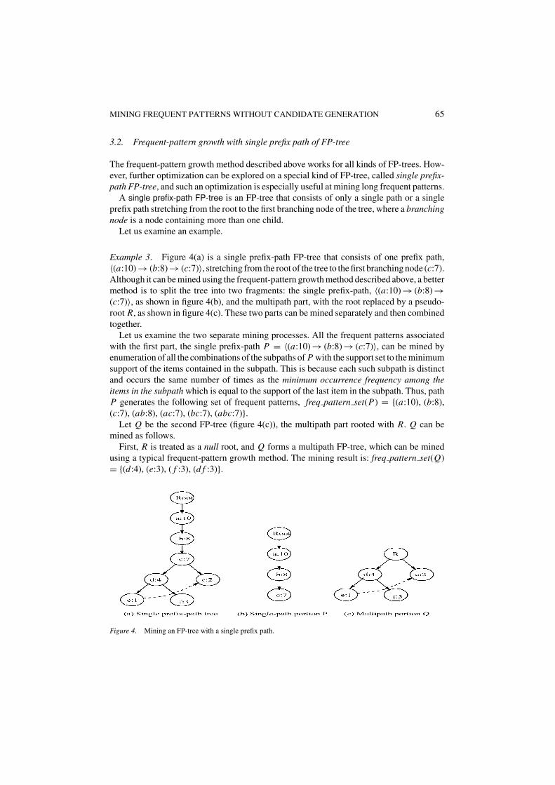
3.2. Frequent-pattern growth with single prefix path of FP-tree

The frequent-pattern growth method described above works for all kinds of FP-trees. How-ever, further optimization can be explored on a special kind of FP-tree, called single prefix-path FP-tree, and such an optimization is especially useful at mining long frequent patterns.

A single prefix-path FP-tree is an FP-tree that consists of only a single path or a singleprefix path stretching from the root to the first branching node of the tree, where a branchingnode is a node containing more than one child.

Let us examine an example.

Example 3. Figure 4(a) is a single prefix-path FP-tree that consists of one prefix path,%(a:10) * (b:8) * (c:7)&, stretching from the root of the tree to the first branching node (c:7).Although it can be mined using the frequent-pattern growth method described above, a bettermethod is to split the tree into two fragments: the single prefix-path, %(a:10) * (b:8) *(c:7)&, as shown in figure 4(b), and the multipath part, with the root replaced by a pseudo-root R, as shown in figure 4(c). These two parts can be mined separately and then combinedtogether.

Let us examine the two separate mining processes. All the frequent patterns associatedwith the first part, the single prefix-path P = %(a:10) * (b:8) * (c:7)&, can be mined byenumeration of all the combinations of the subpaths of P with the support set to the minimumsupport of the items contained in the subpath. This is because each such subpath is distinctand occurs the same number of times as the minimum occurrence frequency among theitems in the subpath which is equal to the support of the last item in the subpath. Thus, pathP generates the following set of frequent patterns, freq pattern set(P) = {(a:10), (b:8),(c:7), (ab:8), (ac:7), (bc:7), (abc:7)}.

Let Q be the second FP-tree (figure 4(c)), the multipath part rooted with R. Q can bemined as follows.

First, R is treated as a null root, and Q forms a multipath FP-tree, which can be minedusing a typical frequent-pattern growth method. The mining result is: freq pattern set(Q)= {(d:4), (e:3), ( f :3), (d f :3)}.

Figure 4. Mining an FP-tree with a single prefix path.

66 HAN ET AL.

Second, for each frequent itemset in Q, R can be viewed as a conditional frequentpattern-base, and each itemset in Q with each pattern generated from R may form a dis-tinct frequent pattern. For example, for (d:4) in freq pattern set(Q), P can be viewed asits conditional pattern-base, and a pattern generated from P , such as (a:10), will generatewith it a new frequent itemset, (ad:4), since a appears together with d at most four times.Thus, for (d:4) the set of frequent patterns generated will be (d:4) . freq pattern set(P) ={(ad:4), (bd:4), (cd:4), (abd:4), (acd:4), (bcd:4), (abcd:4)}, where X . Y means that ev-ery pattern in X is combined with every one in Y to form a “cross-product-like” largeritemset with the support being the minimum support between the two patterns. Thus,the complete set of frequent patterns generated by combining the results of P and Qwill be freq pattern set(Q) . freq pattern set(P), with the support being the support ofthe itemset in Q (which is always no more than the support of the itemsetfrom P).

In summary, the set of frequent patterns generated from such a single prefix path consistsof three distinct sets: (1) freq pattern set(P), the set of frequent patterns generated from thesingle prefix-path, P; (2) freq pattern set(Q), the set of frequent patterns generated fromthe multipath part of the FP-tree, Q; and (3) freq pattern set(Q) . freq pattern set(P), theset of frequent patterns involving both parts.

We first show if an FP-tree consists of a single path P , one can generate the set of frequentpatterns according to the following lemma.

Lemma 3.2 (Pattern generation for an FP-tree consisting of single path). Suppose anFP-tree T consists of a single path P. The complete set of the frequent patterns of T canbe generated by enumeration of all the combinations of the subpaths of P with the supportbeing the minimum support of the items contained in the subpath.

Rationale. Let the single path P of the FP-tree be %a1:s1 * a2:s2 * · · · * ak :sk&. Sincethe FP-tree contains a single path P , the support frequency si of each item ai (for 1 + i + k)is the frequency of ai co-occurring with its prefix string. Thus, any combination of the itemsin the path, such as %ai , . . . , a j & (for 1 + i, j + k), is a frequent pattern, with their co-occurrence frequency being the minimum support among those items. Since every item ineach path P is unique, there is no redundant pattern to be generated with such a combi-national generation. Moreover, no frequent patterns can be generated outside the FP-tree.Therefore, we have the lemma.

We then show if an FP-tree consists of a single prefix-path, the set of frequent patternscan be generated by splitting the tree into two according to the following lemma.

Lemma 3.3 (Pattern generation for an FP-tree consisting of single prefix path). Supposean FP-tree T, similar to the tree in figure 4(a), consists of (1) a single prefix path P, similarto the tree P in figure 4(b), and (2) the multipath part, Q, which can be viewed as anindependent FP-tree with a pseudo-root R, similar to the tree Q in figure 4(c).


The complete set of the frequent patterns of T consists of the following three portions:1. The set of frequent patterns generated from P by enumeration of all the combinations

of the items along path P, with the support being the minimum support among all theitems that the pattern contains.

2. The set of frequent patterns generated from Q by taking root R as “null.”3. The set of frequent patterns combining P and Q formed by taken the cross-product

of the frequent patterns generated from P and Q, denoted as freq pattern set(P) .freq pattern set(Q), that is, each frequent itemset is the union of one frequent itemsetfrom P and one from Q and its support is the minimum one between the supports of thetwo itemsets.

Rationale. Based on the FP-tree construction rules, each node ai in the single prefix pathof the FP-tree appears only once in the tree. The single prefix-path of the FP-tree forms anew FP-tree P , and the multipath part forms another FP-tree Q. They do not share nodesrepresenting the same item. Thus, the two FP-trees can be mined separately.

First, we show that each pattern generated from one of the three portions by followingthe pattern generation rules is distinct and frequent. According to Lemma 3.2, each patterngenerated from P , the FP-tree formed by the single prefix-path, is distinct and frequent.The set of frequent patterns generated from Q by taking root R as “null” is also distinctand frequent since such patterns exist without combining any items in their conditionaldatabases (which are in the items in P . The set of frequent patterns generated by combiningP and Q, that is, taking the cross-product of the frequent patterns generated from P andQ, with the support being the minimum one between the supports of the two itemsets, isalso distinct and frequent. This is because each frequent pattern generated by P can beconsidered as a frequent pattern in the conditional pattern-base of a frequent item in Q,and whose support should be the minimum one between the two supports since this is thefrequency that both patterns appear together.

Second, we show that no patterns can be generated out of this three portions. Sinceaccording to Lemma 3.1, the FP-tree T without being split into two FP-trees P and Q gen-erates the complete set of frequent patterns by pattern growth. Since each pattern generatedfrom T will be generated from either the portion P or Q or their combination, the methodgenerates the complete set of frequent patterns.

3.3. The frequent-pattern growth algorithm

Based on the above lemmas and properties, we have the following algorithm for miningfrequent patterns using FP-tree.

Algorithm 2 (FP-growth: Mining frequent patterns with FP-tree by pattern fragmentgrowth).

Input: A database DB, represented by FP-tree constructed according to Algorithm 1, anda minimum support threshold ! .

Output: The complete set of frequent patterns.

68 HAN ET AL.

Method: call FP-growth(FP-tree, null).

Procedure FP-growth(Tree, "){(1) if Tree contains a single prefix path // Mining single prefix-path FP-tree(2) then {(3) let P be the single prefix-path part of Tree;(4) let Q be the multipath part with the top branching node replaced by a null root;(5) for each combination (denoted as #) of the nodes in the path P do(6) generate pattern # - " with support = minimum support of nodes in #;(7) let freq pattern set(P) be the set of patterns so generated; }(8) else let Q be Tree;(9) for each item ai in Q do { // Mining multipath FP-tree(10) generate pattern # = ai - " with support = ai .support;(11) construct #’s conditional pattern-base and then #’s conditional FP-tree Tree# ;(12) if Tree# /= ,(13) then call FP-growth(Tree#, #);(14) let freq pattern set(Q) be the set of patterns so generated; }(15) return(freq pattern set(P) - freq pattern set(Q) - (freq pattern set(P)

. freq pattern set(Q)))}

Analysis. With the properties and lemmas in Sections 2 and 3, we show that the algorithmcorrectly finds the complete set of frequent itemsets in transaction database DB.

As shown in Lemma 2.1, FP-tree of DB contains the complete information of DB inrelevance to frequent pattern mining under the support threshold ! .

If an FP-tree contains a single prefix-path, according to Lemma 3.3, the generation of thecomplete set of frequent patterns can be partitioned into three portions: the single prefix-pathportion P , the multipath portion Q, and their combinations. Hence we have lines (1)-(4) andline (15) of the procedure. According to Lemma 3.2, the generated patterns for the singleprefix path are the enumerations of the subpaths of the prefix path, with the support being theminimum support of the nodes in the subpath. Thus we have lines (5)-(7) of the procedure.After that, one can treat the multipath portion or the FP-tree that does not contain the singleprefix-path as portion Q (lines (4) and (8)) and construct conditional pattern-base and mineits conditional FP-tree for each frequent itemset ai . The correctness and completeness ofthe prefix path transformation are shown in Property 3.2. Thus the conditional pattern-basesstore the complete information for frequent pattern mining for Q. According to Lemmas 3.1and its corollary, the patterns successively grown from the conditional FP-trees are the setof sound and complete frequent patterns. Especially, according to the fragment growthproperty, the support of the combined fragments takes the support of the frequent itemsetsgenerated in the conditional pattern-base. Therefore, we have lines (9)-(14) of the procedure.Line (15) sums up the complete result according to Lemma 3.3.

Let’s now examine the efficiency of the algorithm. The FP-growth mining process scansthe FP-tree of DB once and generates a small pattern-base Bai for each frequent item ai ,


each consisting of the set of transformed prefix paths of ai . Frequent pattern mining is thenrecursively performed on the small pattern-base Bai by constructing a conditional FP-treefor Bai . As reasoned in the analysis of Algorithm 1, an FP-tree is usually much smaller thanthe size of DB. Similarly, since the conditional FP-tree, “FP-tree | ai ”, is constructed on thepattern-base Bai , it should be usually much smaller and never bigger than Bai . Moreover, apattern-base Bai is usually much smaller than its original FP-tree, because it consists of thetransformed prefix paths related to only one of the frequent items, ai . Thus, each subsequentmining process works on a set of usually much smaller pattern-bases and conditional FP-trees. Moreover, the mining operations consist of mainly prefix count adjustment, countinglocal frequent items, and pattern fragment concatenation. This is much less costly thangeneration and test of a very large number of candidate patterns. Thus the algorithm isefficient.

From the algorithm and its reasoning, one can see that the FP-growth mining process isa divide-and-conquer process, and the scale of shrinking is usually quite dramatic. If theshrinking factor is around 20-100 for constructing an FP-tree from a database, it is expectedto be another hundreds of times reduction for constructing each conditional FP-tree fromits already quite small conditional frequent pattern-base.

Notice that even in the case that a database may generate an exponential number offrequent patterns, the size of the FP-tree is usually quite small and will never grow ex-ponentially. For example, for a frequent pattern of length 100, “a1, . . . , a100”, the FP-treeconstruction results in only one path of length 100 for it, possibly “%a1, * · · · *a100&” (ifthe items are ordered in the list of frequent items as a1, . . . , a100). The FP-growth algorithmwill still generate about 1030 frequent patterns (if time permits!!), such as “a1, a2, . . ., a1a2,. . ., a1a2a3, . . ., a1 . . . a100.” However, the FP-tree contains only one frequent pattern path of100 nodes, and according to Lemma 3.2, there is even no need to construct any conditionalFP-tree in order to find all the patterns.

4. Scaling FP-tree-based FP-growth by database projection

FP-growth proposed in the last section is essentially a main memory-based frequent pat-tern mining method. However, when the database is large, or when the minimum supportthreshold is quite low, it is unrealistic to assume that the FP-tree of a database can fit inmain memory. A disk-based method should be worked out to ensure that mining is highlyscalable. In this section, a method is developed to first partition the database into a set of pro-jected databases, and then for each projected database, construct and mine its correspondingFP-tree.

Let us revisit the mining problem in Example 1.

Example 4. Suppose the FP-tree in figure 1 cannot be held in main memory. Instead ofconstructing a global FP-tree, one can project the transaction database into a set of frequentitem-related projected databases as follows.

Starting at the tail of the frequent item list, p, the set of transactions that contain itemp can be collected into p-projected database. Infrequent items and item p itself can beremoved from them because the infrequent items are not useful in frequent pattern mining,

70 HAN ET AL.

Table 3. Projected databases and their FP-trees.

Item Projected database Conditional FP-tree

p {fcam, cb, fcam} {(c:3)}|p

m {fca, fcab, fca} {( f :3, c:3, a:3)}|mb {fca, f, c} ,a {fc, fc, fc} {( f :3, c:3)}|ac { f, f, f } {( f :3)}|cf , ,

and item p is by default associated with each projected transaction. Thus, the p-projecteddatabase becomes {fcam, cb, fcam}. This is very similar to the the p-conditional pattern-base shown in Table 2 except fcam and fcam are expressed as (fcam:2) in Table 2. Afterthat, the p-conditional FP-tree can be built on the p-projected database based on the FP-treeconstruction algorithm.

Similarly, the set of transactions containing item m can be projected into m-projecteddatabase. Notice that besides infrequent items and item m, item p is also excluded from theset of projected items because item p and its association with m have been considered in thep-projected database. For the same reason, the b-projected database is formed by collectingtransactions containing item b, but infrequent items and items f , m and b are excluded. Thisprocess continues for deriving a-projected database, c-projected database, and so on. Thecomplete set of item-projected databases derived from the transaction database are listed inTable 3, together with their corresponding conditional FP-trees. One can easily see that thetwo processes, construction of the global FP-tree and projection of the database into a setof projected databases, derive identical conditional FP-trees.

As shown in Section 2, a conditional FP-tree is usually orders of magnitude smaller thanthe global FP-tree. Thus, construction of a conditional FP-tree from each projected databaseand then mining on it will dramatically reduce the size of FP-trees to be handled. Whatabout that a conditional FP-tree of a projected database still cannot fit in main memory?One can further project the projected database, and the process can go on recursively untilthe conditional FP-tree fits in main memory.

Let us define the concept of projected database formally.

Definition 2 (Projected database).

– Let ai be a frequent item in a transaction database, DB. The ai -projected database for ai

is derived from DB by collecting all the transactions containing ai and removing fromthem (1) infrequent items, (2) all frequent items after ai in the list of frequent items, and(3) ai itself.

– Let a j be a frequent item in "-projected database. Then the a j"-projected database isderived from the"-projected database by collecting all entries containing a j and removing


from them (1) infrequent items, (2) all frequent items after a j in the list of frequent items,and (3) a j itself.

According to the rules of construction of FP-tree and that of construction of projecteddatabase, the ai -projected database is derived by projecting the same set of items in thetransactions containing ai into the projected database as those collected in the constructionof the ai -subtree in the FP-tree. Thus, the two methods derive the same sets of conditionalFP-trees.

There are two methods for database projection: parallel projection and partition projec-tion.

Parallel projection is implemented as follows: Scan the database to be projected once,where the database could be either a transaction database or an "-projected database. Foreach transaction T in the database, for each frequent item ai in T , project T to the ai -projected database based on the transaction projection rule, specified in the definition ofprojected database. Since a transaction is projected in parallel to all the projected databasesin one scan, it is called parallel projection. The set of projected databases shown in Table 3of Example 4 demonstrates the result of parallel projection. This process is illustrated infigure 5(a).

Parallel projection facilitates parallel processing because all the projected databases areavailable for mining at the end of the scan, and these projected databases can be minedin parallel. However, since each transaction in the database is projected to multiple pro-jected databases, if a database contains many long transactions with multiple frequentitems, the total size of the projected databases could be multiple times of the original one.Let each transaction contains on average l frequent items. A transaction is then projectedto l # 1 projected database. The total size of the projected data from this transaction is1 + 2 + · · · + (l # 1) = l(l#1)

2 . This implies that the total size of the single item-projecteddatabases is about l#1

2 times of that of the original database.To avoid such an overhead, we propose a partition projection method. Partition projection

is implemented as follows. When scanning the database (original or "-projected) to beprojected, a transaction T is projected to the ai -projected database only if ai is a frequentitem in T and there is no any other item after ai in the list of frequent items appearing

Figure 5. Parallel projection vs. partition projection.

72 HAN ET AL.

in the transaction. Since a transaction is projected to only one projected database at thedatabase scan, after the scan, the database is partitioned by projection into a set of projecteddatabases, and hence it is called partition projection.

The projected databases are mined in the reversed order of the list of frequent items. Thatis, the projected database of the least frequent item is mined first, and so on. Each time whena projected database is being processed, to ensure the remaining projected databases obtainthe complete information, each transaction in it is projected to the a j -projected database,where a j is the item in the transaction such that there is no any other item after a j in thelist of frequent items appearing in the transaction. The partition projection process for thedatabase in Example 4 is illustrated in figure 5(b).

The advantage of partition projection is that the total size of the projected databases ateach level is smaller than the original database, and it usually takes less memory and I/Os tocomplete the partition projection. However, the processing order of the projected databasesbecomes important, and one has to process these projected databases in a sequential manner.Also, during the processing of each projected database, one needs to project the processedtransactions to their corresponding projected databases, which may take some I/O as well.Nevertheless, due to its low memory requirement, partition projection is still a promisingmethod in frequent pattern mining.

Example 5. Let us examine how the database in Example 4 can be projected by partitionprojection.

First, by one scan of the transaction database, each transaction is projected to only oneprojected database. The first transaction, facdgimp, is projected to the p-projected databasesince p is the last frequent item in the list of frequent items. Thus, fcam (i.e., with infrequentitems removed) is inserted into the p-projected database. Similarly, transaction abcflmo isprojected to the m-projected database as fcab, bfhjo to the b-projected database as f ,bcksp to the p-projected database as cb, and finally, afcelpmn to the p-projected databaseas fcam. After this phrase, the entries in every projected databases are shown in Table 4.

With this projection, the original database can be replaced by the set of single-itemprojected databases, and the total size of them is smaller than that of the original database.

Second, the p-projected database is first processed (i.e., construction of p-conditionalFP-tree), where p is the last item in the list of frequent items. During the processing of thep-projected database, each transaction is projected to the corresponding projected database

Table 4. Single-item projected databases by partition projection.

Item Projected databases

p {fcam, cb, fcam}m {fcab}b { f }a ,c ,f ,


according to the same partition projection rule. For example, fcam is projected to the m-projected database as fca, cb is projected to the b-projected database as c, and so on. Theprocess continues until every single-item projected database is completely processed.

5. Experimental evaluation and performance study

In this section, we present a performance comparison of FP-growth with the classicalfrequent pattern mining algorithm Apriori, and an alternative database projection-based al-gorithm, TreeProjection. We first give a concise introduction and analysis to TreeProjection,and then report our experimental results.

5.1. A comparative analysis of FP-growth and TreeProjection methods

The TreeProjection algorithm proposed by Agarwal et al. (2001) constructs a lexicographicaltree and projects a large database into a set of reduced, item-based sub-databases basedon the frequent patterns mined so far. Since it applies a tree construction method andperforms mining recursively on progressively smaller databases, it shares some similaritieswith FP-growth. However, the two methods have some fundamental differences in treeconstruction and mining methodologies, and will lead to notable differences on efficiencyand scalability. We will explain such similarities and differences by working through thefollowing example.

Example 6. For the same transaction database presented in Example 1, we construct thelexicographic tree according to the method described in Agarwal et al. (2001). The resulttree is shown in figure 6, and the construction process is presented as follows.

By scanning the transaction database once, all frequent 1-itemsets are identified. Asrecommended in Agarwal et al. (2001), the frequency ascending order is chosen as the

Figure 6. A lexicographical tree built for the same transactional database DB.

74 HAN ET AL.

ordering of the items. So, the order is p-m-b-a-c-f , which is exactly the reverse order ofwhat is used in the FP-tree construction. The top level of the lexicographic tree is constructed,i.e. the root and the nodes labeled by length-1 patterns. At this stage, the root node labeled“null” and all the nodes which store frequent 1-itemsets are generated. All the transactionsin the database are projected to the root node, i.e., all the infrequent items are removed.

Each node in the lexicographical tree contains two pieces of information: (i) the patternthat node represents, and (ii) the set of items that may generate longer patterns by addingthem to the pattern. The latter piece information is recorded as active extensions and activeitems.

Then, a matrix at the root node is created, as shown below. The matrix computes thefrequencies of length-2 patterns, thus all pairs of frequent items are included in the matrix.The items in pairs are arranged in the ordering. The matrix is built by adding counts fromevery transaction, i.e., computing frequent 2-itemsets based on transactions stored in theroot node.

p m b a c f

p

m 2

b 1 1

a 2 3 1

c 3 3 2 3

f 2 3 2 3 3

At the same time of building the matrix, transactions in the root are projected to level-1nodes as follows. Let t = a1a2 . . . an be a transaction with all items listed in ordering. t isprojected to node ai (1 + i < n # 1) as t )

ai= ai+1ai+2 . . . an .

From the matrix, all the frequent 2-itemsets are found as: {pc, ma, mc, mf , ac, af , cf }.The nodes in lexicographic tree for them are generated. At this stage, the only nodesfor 1-itemsets which are active are those for m and a, because only they contain enoughdescendants to potentially generate longer frequent itemsets. All nodes up to and includinglevel-1 except for these two nodes are pruned.

In the same way, the lexicographic tree is grown level by level. From the matrix at nodem, nodes labeled mac, ma f, and mcf are added, and only ma is active in all the nodes forfrequent 2-itemsets. It is easy to see that the lexicographic tree in total contains 19 nodes.

The number of nodes in a lexicographic tree is exactly that of the frequent itemsets.TreeProjection proposes an efficient way to enumerate frequent patterns. The efficiency ofTreeProjection can be explained by two main factors: (1) the transaction projection limitsthe support counting in a relatively small space, and only related portions of transactionsare considered; and (2) the lexicographical tree facilitates the management and counting ofcandidates and provides the flexibility of picking efficient strategy during the tree genera-tion phase as well as transaction projection phase. Agarwal et al. (2001) reports that theiralgorithm is up to one order of magnitude faster than other recent techniques in literature.


However, in comparison with the FP-growth method, TreeProjection suffers from someproblems related to efficiency, and scalability. We analyze them as follows.

First, TreeProjection may encounter difficulties at computing matrices when the databaseis huge, when there are a lot of transactions containing many frequent items, and/or when thesupport threshold is very low. This is because in such cases there often exist a large numberof frequent items. The size of the matrices at high level nodes in the lexicographical tree canbe huge, as shown in our introduction section. The study in TreeProjection (Agarwal et al.,2001) has developed some smart memory caching methods to overcome this problem.However, it could be wise not to generate such huge matrices at all instead of findingsome smart caching techniques to reduce the cost. Moreover, even if the matrix can becached efficiently, its computation still involves some nontrivial overhead. To compute amatrix at node P with n projected transactions, the cost is O(

!ni=1

|Ti |22 ), where |Ti | is

the length of the transaction. If the number of transaction is large and the length of eachtransaction is long, the computation is costly. The FP-growth method will never need tobuild up matrices and compute 2-itemset frequency since it avoids the generation of anycandidate k-itemsets for any k by applying a pattern growth method. Pattern growth can beviewed as successive computation of frequent 1-itemset (of the database and conditionalpattern bases) and assembling them into longer patterns. Since computing frequent 1-itemsets is much less expensive than computing frequent 2-itemsets, the cost is substantiallyreduced.

Second, since one transaction may contain many frequent itemsets, one transaction inTreeProjection may be projected many times to many different nodes in the lexicographicaltree. When there are many long transactions containing numerous frequent items, transactionprojection becomes a nontrivial cost of TreeProjection. The FP-growth method constructsFP-tree which is a highly compact form of transaction database. Thus both the size and thecost of computation of conditional pattern bases, which corresponds roughly to the compactform of projected transaction databases, are substantially reduced.

Third, TreeProjection creates one node in its lexicographical tree for each frequent item-set. At the first glance, this seems to be highly compact since FP-tree does not ensure thateach frequent node will be mapped to only one node in the tree. However, each branch of theFP-tree may store many “hidden” frequent patterns due to the potential generation of manycombinations using its prefix paths. Notice that the total number of frequent k-itemsets canbe very large in a large database or when the database has quite long frequent itemsets.For example, for a frequent itemset (a1, a2, . . . , a100), the number of frequent itemsets atthe 50th-level of the lexicographic tree will be ( 100

50 ) = 100!50!.50! $ 1.0 . 1029. For the same

frequent itemset, FP-tree and FP-growth will only need one path of 100 nodes.In summary, FP-growth mines frequent itemsets by (1) constructing highly compact

FP-trees which share numerous “projected” transactions and hide (or carry) numerousfrequent patterns, and (2) applying progressive pattern growth of frequent 1-itemsets whichavoids the generation of any potential combinations of candidate itemsets implicitly orexplicitly, whereas TreeProjection must generate candidate 2-itemsets for each projecteddatabase. Therefore, FP-growth is more efficient and more scalable than TreeProjection,especially when the number of frequent itemsets becomes really large. These observationsand analyses are well supported by our experiments reported in this section.

76 HAN ET AL.

5.2. Environments of experiments

All the experiments are performed on a 266-MHz Pentium PC machine with 128 megabytesmain memory, running on Microsoft Windows/NT. All the programs are written in Mi-crosoft/Visual C++6.0. Notice that we do not directly compare our absolute number ofruntime with those in some published reports running on the RISC workstations becausedifferent machine architectures may differ greatly on the absolute runtime for the samealgorithms. Instead, we implement their algorithms to the best of our knowledge based onthe published reports on the same machine and compare in the same running environment.Please also note that run time used here means the total execution time, that is, the pe-riod between input and output, instead of CPU time measured in the experiments in someliterature. We feel that run time is a more comprehensive measure since it takes the totalrunning time consumed as the measure of cost, whereas CPU time considers only the costof the CPU resource. Also, all reports on the runtime of FP-growth include the time ofconstructing FP-trees from the original databases.

The experiments are pursued on both synthetic and real data sets. The synthetic datasets which we used for our experiments were generated using the procedure described inAgrawal and Srikant (1994). We refer readers to it for more details on the generation ofdata sets.

We report experimental results on two synthetic data sets. The first one is T10.I4.D100Kwith 1K items. In this data set, the average transaction size and average maximal potentiallyfrequent itemset size are set to 10 and 4, respectively, while the number of transactions inthe dataset is set to 100 K. It is a sparse dataset. The frequent itemsets are short and notnumerous.

The second synthetic data set we used is T25.I20.D100K with 10 K items. The averagetransaction size and average maximal potentially frequent itemset size are set to 25 and 20,respectively. There exist exponentially numerous frequent itemsets in this data set whenthe support threshold goes down. There are also pretty long frequent itemsets as well asa large number of short frequent itemsets in it. It contains abundant mixtures of short andlong frequent itemsets.

To test the capability of FP-growth on dense datasets with long patterns, we use thereal data set Connect-4, compiled from the Connect-4 game state information. The data setis from the UC-Irvine Machine Learning Database Repository (http://www.ics.uci.edu/0mlearn/MLRepository.html). It contains 67, 557 transactions, while each transaction is with43 items. It is a dense dataset with a lot of long frequent itemsets.

5.3. Compactness of FP-tree

To test the compactness of FP-trees, we compare the sizes of the following structures.

– Alphabetical FP-tree. It includes the space of all the links. However, in such an FP-tree,the alphabetical order of items are used instead of frequency descending order.

– Ordered FP-tree. Again, the size covers that of all links. In such an FP-tree, the items aresorted according to frequency descending order.


Figure 7. Compactness of FP-tree over data set Connect-4.

– Transaction database. Each item in a transaction is stored as an integer. It is simply thesum of occurrences of items in transactions.

– Frequent transaction database. That is the sub-database extracted from the original oneby removing all infrequent items.

In real dataset Connect-4, FP-tree achieves good compactness. As seen from the resultshown in figure 7, the size of ordered FP-tree is always smaller than the size of the transactiondatabase and the frequent transaction database. In a dense database, the size of the databaseand that of its frequent database are close. The size of the alphabetical FP-tree is smaller thanthat of the two databases in most cases but is slightly larger (about 1.5 to 2.5 times larger)than the size of the ordered FP-tree. It indicates that the frequency-descending ordering ofthe items benefits data compression in this case.

In dataset T25.I20.D100k, which contains abundant mixture of long and short frequentpatterns, FP-tree is compact most of the time. The result is shown in figure 8. Only when

Figure 8. Compactness of FP-tree over data set T25.I20.D100k.

78 HAN ET AL.

Figure 9. Compactness of FP-tree over data set T10.I4.D100k.

the support threshold lower than 2.5%, is the size of FP-tree larger than that of frequentdatabase. Moreover, as long as the support threshold is over 1.5%, the FP-tree is smallerthan the transaction database. The difference of sizes of ordered FP-tree and alphabeticalFP-tree is quite small in this dataset. It is about 2%.

In sparse dataset T10.I4.D100k, FP-tree achieves good compactness when the supportthreshold is over 3.5%. Again, the difference of ordered FP-tree and alphabetical FP-tree istrivial. The result is shown in figure 9.

The above experiments lead to the following conclusions.

– FP-tree achieves good compactness most of the time. Especially in dense datasets, itcan compress the database many times. Clearly, there is some overhead for pointers andcounters. However, the gain of sharing among frequent projections of transactions issubstantially more than the overhead and thus makes FP-tree space more efficient inmany cases.

– When support is very low, FP-tree becomes bushy. In such cases, the degree of sharingin branches of FP-tree becomes low. The overhead of links makes the size of FP-treelarge. Therefore, instead of building FP-tree, we should construct projected databases.That is the reason why we build FP-tree for transaction database/projected database onlywhen it passes certain density threshold. From the experiments, one can see that such athreshold is pretty low, and easy to touch. Therefore, even for very large and/or sparsedatabase, after one or a few rounds of database projection, FP-tree can be used for all theremaining mining tasks.

In the following experiments, we employed an implementation of FP-growth that inte-grates both database projection and FP-tree mining. The density threshold is set to 3%, anditems are listed in frequency descending order.

5.4. Scalability study

The runtime of Apriori, TreeProjection, and FP-growth on synthetic data set T10.I4.D100Kas the support threshold decreases from 0.15% to 0.01% is shown in figure 10.


Figure 10. Scalability with threshold over sparse data set.

FP-growth is faster than both Apriori and TreeProjection. TreeProjection is faster andmore scalable than Apriori. Since the dataset is sparse, as the support threshold is high,the frequent itemsets are short and the set of such itemsets is not large, the advantages ofFP-growth and TreeProjection over Apriori are not so impressive. However, as the supportthreshold goes down, the gap becomes wider. FP-growth can finish the computation forsupport threshold 0.01% within the time for Apriori over 0.05%. TreeProjection is alsoscalable, but is slower than FP-growth.

The advantages of FP-growth over Apriori becomes obvious when the dataset containsan abundant number of mixtures of short and long frequent patterns. Figure 11 shows theexperimental results of scalability with threshold over dataset T25.I20.D100k. FP-growthcan mine with support threshold as low as 0.05%, with which Apriori cannot work outwithin reasonable time. TreeProjection is also scalable and faster than Apriori, but is slowerthan FP-growth.

Figure 11. Scalability with threshold over dataset with abundant mixtures of short and long frequent patterns.

80 HAN ET AL.

Figure 12. Scalability with threshold over Connect-4.

The advantage of FP-growth is dramatic in datasets with long patterns, which is challeng-ing to the algorithms that mine the complete set of frequent patterns. The result on miningthe real dataset Connect-4 is shown in figure 12. To the best of our knowledge, this is thefirst algorithm that handles such dense real dataset in performance study. From the figure,one can see that FP-growth is scalable even when there are many long patterns. Withoutcandidate generation, FP-growth enumerates long patterns efficiently. In such datasets, nei-ther Apriori nor TreeProjection are comparable to the performance of FP-growth. To dealwith long patterns, Apriori has to generate a tremendous number of candidates, that is verycostly. The main costs in TreeProjection are matrix computation and transaction projection.In a database with a large number of frequent items, the matrices become quite large, andthe computation cost jumps up substantially. In contrast, the height of FP-tree is limited bythe maximal length of the transactions, and many transactions share the prefix paths of anFP-tree. This explains why FP-growth has distinct advantages when the support thresholdis low and when the number of transactions is large.

To test the scalability of FP-growth against the number of transactions, a set of syntheticdatasets are generated using the same parameters of T10.I4 and T25.I20, and the numberof transactions ranges from 100 k to 1 M. FP-growth is tested over them using the samesupport threshold in percentage. The result is in figure 13, which shows the linear increaseof runtime with the number of transactions. Please note that unlike the way reported in someliterature, we do not replicate transactions in real data sets to test the scalability. This isbecause no matter how many times the transactions are replicated, FP-growth builds up anFP-tree with the size identical to that of the original (nonreplicated) one, and the scaling-upof such databases becomes trivial.

6. Discussions

The frequent-pattern growth method introduced here represents an interesting approach forscalable frequent-pattern mining. In this section, we discuss some additional issues relatedto its implementation, usage, and extension.


Figure 13. Scalability of FP-growth with number of transactions.

6.1. Materialization and maintenance of FP-trees

Although we have studied the dynamic generation of FP-trees, it is possible to materializeand incrementally update an FP-tree. We examine the related issues here.

6.1.1. Construction of disk-resident FP-trees. When the database grows very large, itis unrealistic to construct a main memory-based FP-tree. Database projection has beenintroduced in Section 3.4 as an effective approach. An interesting alternative is to constructa disk-resident FP-tree.

The B+-tree structure, popularly used in relational database systems, can be used to indexFP-tree as well. Since there are many operations localized to single paths or individualitem prefix sub-trees, such as pattern matching for node insertion, creation of transformedprefix paths for each node ai , etc., it is important to cluster FP-tree nodes according to thetree/subtree structure. That is, one should (1) store each item prefix sub-tree on the samepage, if possible, or at least on a sequence of continuous pages on disk; (2) store eachsubtree on the same page, and put the shared prefix path as the header information of thepage; and (3) cluster the node-links belonging to the same paged nodes together, etc. Thisalso facilitates a breadth-first search fashion for mining all the patterns starting from all thenodes in the header in parallel.

To reduce the I/O costs by following node-links, mining should be performed in a groupaccessing mode, that is, when accessing nodes following node-links, one should exhaustthe node traversal tasks in main memory before fetching the nodes on disks.

Notice that one may also construct node-link-free FP-trees. In this case, when traversinga tree path, one should project the prefix subpaths of all the nodes into the correspondingconditional pattern bases. This is feasible if both FP-tree and one page of each of its one-level conditional pattern bases can fit in memory. Otherwise, additional I/Os will be neededto swap in and out the conditional pattern bases.

6.1.2. Materialization of an FP-tree for frequent-pattern mining. Although an FP-treeis rather compact, its construction needs two scans of a transaction database, which may

82 HAN ET AL.

represent a nontrivial overhead. It could be beneficial to materialize an FP-tree for regularfrequent pattern mining.

One difficulty for FP-tree materialization is how to select a good minimum support thresh-old ! in materialization since ! is usually query-dependent. To overcome this difficulty, onemay use a low ! that may usually satisfy most of the mining queries in the FP-tree con-struction. For example, if we notice that 98% queries have ! " 20, we may choose ! = 20as the FP-tree materialization threshold: that is, only 2% of queries may need to construct anew FP-tree. Since an FP-tree is organized in the way that less frequently occurring itemsare located at the deeper paths of the tree, it is easy to select only the upper portions of theFP-tree (or drop the low portions which do not satisfy the support threshold) when miningthe queries with higher thresholds. Actually, one can directly work on the materializedFP-tree by starting at an appropriate header entry since one just need to get the prefix pathsno matter how low support the original FP-tree is.

6.1.3. Incremental update of an FP-tree. Another issue related to FP-tree materializationis how to incrementally update an FP-tree, such as when adding daily new transactions intoa database containing records accumulated for months.

If the materialized FP-tree takes 1 as its minimum support (i.e., it is just a compact versionof the original database), the update will not cause any problem since adding new records isequivalent to scanning additional transactions in the FP-tree construction. However, a fullFP-tree may be an undesirably large. Thus setting 1 as its minimum support may not be agood solution.

In the general case, we can register the occurrence frequency of every items in F1 andtrack them in updates. This is not too costly but it benefits the incremental updates of anFP-tree as follows. Suppose an FP-tree was constructed based on a validity support threshold(called “watermark”) $ = 0.1% in a DB with 108 transactions. Suppose an additional 106

transactions are added in. The frequency of each item is updated. If the highest relativefrequency among the originally infrequent items (i.e., not in the FP-tree) goes up to, say12%, the watermark will need to go up accordingly to $ > 0.12% to exclude such item(s).However, with more transactions added in, the watermark may even drop since an item’srelative support frequency may drop with more transactions added in. Only when the FP-treewatermark is raised to some undesirable level, the reconstruction of the FP-tree for the newDB becomes necessary.

6.2. Extensions of frequent-pattern growth method in data mining

The philosophy of database compression and partition-based frequent-pattern mining canbe extended to constraint-based mining and mining other kinds of frequent patterns, suchas max-patterns, sequential patterns.

6.2.1. FP-tree mining with constraints. Constraint-based frequent-pattern mining repre-sents an important direction towards user-controlled data mining. Constraint-based asso-ciation mining using the Apriori-like mining methodology has been studied extensively(Srikant et al., 1997; Ng et al., 1998). With the introduction of FP-growth method, one


may wonder whether constraint-based mining may benefit with FP-tree-like structures. Athorough study of this issue, such as classification of various kinds of constraints and devel-opment of methods of FP-tree-based mining with sophisticated constraints, such as thosein Ng et al. (1998), should be the task of another research paper.2 Here we only showhow to apply FP-tree structure to mining frequent patterns by incorporation of constraintsassociated with a set of items.

Suppose one may just like to derive frequent patterns only associated with a particularset of items, S, such as mining the set of frequent patterns containing c or m in Example 1.Instead of mining frequent patterns for all the frequent items, one may explore the FP-tree-based mining as follows. With the same FP-tree, the FP-growth mining method may justneed to be modified minorly. The only additional care is when computing a transformedprefix path for an item m, one also needs to look down the path to include the items, suchas p, which are not in S. Our previous computation for the whole database will not needto consider m’s pairing with p since it would have been checked when examining node p.However, since p is not in S now, such a pair would have been missed if m’s computationdid not look down the path to include p.

6.2.2. FP-tree mining of other frequent patterns. FP-tree-based mining method can beextended to mining many other kinds of interesting frequent patterns. We examine a fewsuch examples.

The first example is on mining frequent closed itemsets. Since frequent pattern miningoften generates a very large number of frequent itemsets, it hinders the effectiveness ofmining since users have to sift through a large number of mined rules to find useful ones.An interesting alternative method proposed recently by Pasquier et al. (1999) is to minefrequent closed itemsets, where an itemset " is a closed itemset if there exists no propersuperset of " that has the same support as " in the database. Mining frequent closed itemsetshas the same power as mining the complete set of frequent itemsets, but it may substantiallyreduce redundant rules to be generated and increase the effectiveness of mining. A study atmining closed items using an Apriori-like philosophy but adopting a vertical data format,i.e., viewing database as “(item id: a set of transactions)” instead of “(transaction id: a setof items),” has been studied in Zaki and Hsiao (2002). The FP-tree-based frequent-patterngrowth method can be extended and further optimized for mining such closed itemsets,which has been reported in our subsequent study, as a new closed pattern mining algorithm,called CLOSET (Pei et al., 2000).

The second example is on mining sequential patterns. A sequential patterns is a frequentpattern in an event sequence database where a sequence is a set of events happening atdifferent times. Most of the previously developed sequential pattern mining methods, suchas Agrawal and Srikant (1995), Srikant and Agrawal (1996) and Mannila et al. (1997), followthe methodology of Apriori since the Apriori-based method may substantially reduce thenumber of combinations to be examined. However, Apriori still encounters problems when asequence database is large and/or when sequential patterns to be mined are numerous and/orlong. Our frequent-pattern growth method can be extended to mining sequential patternsusing the ideas of projection of sequence database and growth of subsequence fragmentsto confine search space. An efficient sequential pattern method, called PrefixSpan (Pei

84 HAN ET AL.

et al., 2001), has been developed in this direction and our performance study has shown asubstantial performance improvement over the Apriori-based GSP algorithm (Srikant andAgrawal, 1996).

7. Conclusions

We have proposed a novel data structure, frequent pattern tree (FP-tree), for storing com-pressed, crucial information about frequent patterns, and developed a pattern growth method,FP-growth, for efficient mining of frequent patterns in large databases.

There are several advantages of FP-growth over other approaches: (1) It constructs ahighly compact FP-tree, which is usually substantially smaller than the original databaseand thus saves the costly database scans in the subsequent mining processes. (2) It appliesa pattern growth method which avoids costly candidate generation and test by successivelyconcatenating frequent 1-itemset found in the (conditional) FP-trees. This ensures that itnever generates any combinations of new candidate sets which are not in the databasebecause the itemset in any transaction is always encoded in the corresponding path ofthe FP-trees. In this context, mining is not Apriori-like (restricted) generation-and-test butfrequent pattern (fragment) growth only. The major operations of mining are count accumu-lation and prefix path count adjustment, which are usually much less costly than candidategeneration and pattern matching operations performed in most Apriori-like algorithms.(3) It applies a partitioning-based divide-and-conquer method which dramatically reducesthe size of the subsequent conditional pattern bases and conditional FP-tree. Several otheroptimization techniques, including direct pattern generation for single tree-path and em-ploying the least frequent events as suffix, also contribute to the efficiency of the method.

We have implemented the FP-growth method, studied its performance in comparison withseveral influential frequent pattern mining algorithms in large databases. Our performancestudy shows that the method mines both short and long patterns efficiently in large databases,outperforming the current candidate pattern generation-based algorithms. The FP-growthmethod has also been implemented in the DBMiner system and been tested in large industrialdatabases, such as a retail chain database, with satisfactory performance.

Since our first publication of FP-growth method for mining frequent patterns withoutcandidate generation (Han et al., 2000), there have been many subsequent studies on im-provements of performance of frequent patterns based on the pattern-growth philosophy, aswell as extension of the scope of the method to cover other kinds of pattern mining tasks.The pattern-growth framework has been extended towards (1) mining closed itemsets asproposed in the CLOSET algorithm (Pei et al., 2000), (2) mining sequential patterns as pro-posed in the PrefixSpan algorithm (Pei et al., 2001), and (3) pushing tough constraints deepinto frequent pattern mining processes (Pei et al., 2001). Moreover, a notable effort is theproposal of the H-mine algorithm (Pei et al., 2001) for mining frequent patterns efficientlyin sparse data sets. FP-growth, though efficient at mining dense data sets, may incur un-necessary overhead due to its recursive construction of FP-trees. Following the philosophyof frequent pattern growth, but not constructing FP-trees, the H-mine algorithm constructsanother data structure, called H-struct, and mines directly on the H-struct without recursivegeneration of numerous conditional FP-trees. The experiments reported in Pei et al. (2001)


shows that H-mine outperforms FP-growth when database is sparse. A suggested approachis to integrate the two algorithms and dynamically select the FP-tree-based and H-struct-based algorithms based on the characteristics of current data distribution. Recently, somestudies also show that various FP-tree mining strategies (such as bottom-up vs. top-downmethods) may lead to different efficiency over data sets of different data distributions.

There are still many interesting research issues related to the extensions of pattern-growthapproach, such as mining structured patterns by further development of the frequent pattern-growth approach, mining approximate or fault-tolerant patterns in noisy environments,frequent-pattern-based clustering and classification, and so on.

Acknowledgments

We would like to express our thanks to anonymous reviewers of our conference and journalsubmissions on this theme. Their constructive comments have improved the quality of thiswork.

Notes

1. Notice that support is defined here as absolute occurrence frequency, not the relative one as in some literature.2. One such study has been performed by us in Pei et al. (2001).

References

Agarwal, R., Aggarwal, C., and Prasad, V.V.V. 2001. A tree projection algorithm for generation of frequentitemsets. Journal of Parallel and Distributed Computing, 61:350–371,

Agrawal, R., Imielinski, T., and Swami, A. 1993. Mining association rules between sets of items in large databases.In Proc. 1993 ACM-SIGMOD Int. Conf. Management of Data (SIGMOD’93), Washington, DC, pp. 207–216.

Agrawal, R., Mannila, H., Srikant, R., Toivonen, H., and Verkamo, A.I. 1996. Fast discovery of association rules.In Advances in Knowledge Discovery and Data Mining, U.M. Fayyad, G. Piatetsky-Shapiro, P. Smyth, and R.Uthurusamy (Eds.), AAAI/MIT Press, pp. 307–328.

Agrawal, R. and Srikant, R. 1994. Fast algorithms for mining association rules. In Proc. 1994 Int. Conf. VeryLarge Data Bases (VLDB’94), Santiago, Chile, pp. 487–499.

Agrawal, R. and Srikant, R. 1995. Mining sequential patterns. In Proc. 1995 Int. Conf. Data Engineering (ICDE’95),Taipei, Taiwan, pp. 3–14.

Bayardo, R.J. 1998. Efficiently mining long patterns from databases. In Proc. 1998 ACM-SIGMOD Int. Conf.Management of Data (SIGMOD’98), Seattle, WA, pp. 85–93.

Brin, S., Motwani, R., and Silverstein, C. 1997. Beyond market basket: Generalizing association rules to cor-relations. In Proc. 1997 ACM-SIGMOD Int. Conf. Management of Data (SIGMOD’97), Tucson, Arizona,pp. 265–276.

Dong, G. and Li, J. 1999. Efficient mining of emerging patterns: Discovering trends and differences. In Proc. 1999Int. Conf. Knowledge Discovery and Data Mining (KDD’99), San Diego, CA, pp. 43–52.

Grahne, G., Lakshmanan, L., and Wang, X. 2000. Efficient mining of constrained correlated sets. In Proc. 2000Int. Conf. Data Engineering (ICDE’00), San Diego, CA, pp. 512–521.

Han, J., Dong, G., and Yin, Y. 1999. Efficient mining of partial periodic patterns in time series database. In Proc.1999 Int. Conf. Data Engineering (ICDE’99), Sydney, Australia, pp. 106–115.

Han, J., Pei, J., and Yin, Y. 2000. Mining frequent patterns without candidate generation. In Proc. 2000 ACM-SIGMOD Int. Conf. Management of Data (SIGMOD’00), Dallas, TX, pp. 1–12.

86 HAN ET AL.

Kamber, M., Han, J., and Chiang, J.Y. 1997. Metarule-guided mining of multi-dimensional association rules usingdata cubes. In Proc. 1997 Int. Conf. Knowledge Discovery and Data Mining (KDD’97), Newport Beach, CA,pp. 207–210.

Lent, B., Swami, A., and Widom, J. 1997. Clustering association rules. In Proc. 1997 Int. Conf. Data Engineering(ICDE’97), Birmingham, England, pp. 220–231.

Mannila, H., Toivonen, H., and Verkamo, A.I. 1994. Efficient algorithms for discovering association rules. In Proc.AAAI’94 Workshop Knowledge Discovery in Databases (KDD’94), Seattle, WA, pp. 181–192.

Mannila, H., Toivonen, H., and Verkamo, A.I. 1997. Discovery of frequent episodes in event sequences. DataMining and Knowledge Discovery, 1:259–289.

Ng, R., Lakshmanan, L.V.S., Han, J., and Pang, A. 1998. Exploratory mining and pruning optimizations ofconstrained associations rules. In Proc. 1998 ACM-SIGMOD Int. Conf. Management of Data (SIGMOD’98),Seattle, WA, pp. 13–24.

Pasquier, N., Bastide, Y., Taouil, R., and Lakhal, L. 1999. Discovering frequent closed itemsets for associationrules. In Proc. 7th Int. Conf. Database Theory (ICDT’99), Jerusalem, Israel, pp. 398–416.

Park, J.S., Chen, M.S., and Yu, P.S. 1995. An effective hash-based algorithm for mining association rules. In Proc.1995 ACM-SIGMOD Int. Conf. Management of Data (SIGMOD’95), San Jose, CA, pp. 175–186.

Pei, J., Han, J., and Lakshmanan, L.V.S. 2001. Mining frequent itemsets with convertible constraints. In Proc.2001 Int. Conf. Data Engineering (ICDE’01), Heidelberg, Germany, pp. 433–332.

Pei, J., Han, J., Lu, H., Nishio, S., Tang, S., and Yang, D. 2001. H-Mine: Hyper-structure mining of frequentpatterns in large databases. In Proc. 2001 Int. Conf. Data Mining (ICDM’01), San Jose, CA, pp. 441–448.

Pei, J., Han, J., and Mao, R. 2000. CLOSET: An efficient algorithm for mining frequent closed itemsets. InProc. 2000 ACM-SIGMOD Int. Workshop Data Mining and Knowledge Discovery (DMKD’00), Dallas, TX,pp. 11–20.

Pei, J., Han, J., Mortazavi-Asl, B., Pinto, H., Chen, Q., Dayal, U., and Hsu, M.-C. 2001. PrefixSpan: Miningsequential patterns efficiently by prefix-projected pattern growth. In Proc. 2001 Int. Conf. Data Engineering(ICDE’01), Heidelberg, Germany, pp. 215–224.

Srikant, R. and Agrawal, R. 1996. Mining sequential patterns: Generalizations and performance improvements.In Proc. 5th Int. Conf. Extending Database Technology (EDBT’96), Avignon, France, pp. 3–17.

Silverstein, C., Brin, S., Motwani, R., and Ullman, J. 1998. Scalable techniques for mining causal structures. InProc. 1998 Int. Conf. Very Large Data Bases (VLDB’98), New York, NY, pp. 594–605.

Savasere, A., Omiecinski, E., and Navathe, S. 1995. An efficient algorithm for mining association rules in largedatabases. In Proc. 1995 Int. Conf. Very Large Data Bases (VLDB’95), Zurich, Switzerland, pp. 432–443.

Sarawagi, S., Thomas, S., and Agrawal, R. 1998. Integrating association rule mining with relational databasesystems: Alternatives and implications. In Proc. 1998 ACM-SIGMOD Int. Conf. Management of Data (SIG-MOD’98), Seattle, WA, pp. 343–354.

Srikant, R., Vu, Q., and Agrawal, R. 1997. Mining association rules with item constraints. In Proc. 1997 Int. Conf.Knowledge Discovery and Data Mining (KDD’97), Newport Beach, CA, pp. 67–73.

Zaki, M.J. and Hsiao, C.J. 2002. CHARM: An efficient algorithm for closed itemset mining. In Proc. 2002 SIAMInt. Conf. Data Mining, Arlington, VA, pp. 457–473.

Jiawei Han is a Professor in the Department of Computer Science at the University of Illinois at Urbana-Champaign. Previously, he was an Endowed University Professor at Simon Fraser University, Canada. He hasbeen working on research into data mining, data warehousing, spatial and multimedia databases, deductive andobject-oriented databases, and bio-medical databases, with over 250 journal and conference publications. He haschaired or served in over 90 program committees of international conferences and workshops. He also servedor is serving on the editorial boards for Data Mining and Knowledge Discovery: An International Journal, IEEETransactions on Knowledge and Data Engineering, and Journal of Intelligent Information Systems. He is currentlyserving on the Board of Directors for the Executive Committee of ACM Special Interest Group on KnowledgeDiscovery and Data Mining (SIGKDD) and chairman of ACM SIGKDD Curriculum Committee. Jiawei has re-ceived IBM Faculty Awards, the Outstanding Contribution Award at the 2002 International Conference on DataMining, and an ACM Service Award.


Jian Pei received the B.Eng. and the M.Eng. degrees, both in Computer Science, from Shanghai Jiao TongUniversity, China, in 1991 and 1993, respectively, and the Ph.D. degree in Computing Science from Simon FraserUniversity, Canada, in 2002. He was a Ph.D. candidate in Peking University in 1997–1999. He is currently anAssistant Professor of Computer Science and Engineering, the State University of New York at Buffalo, USA.His research interests include data mining, data warehousing, online analytical processing, database systems, andbio-informatics. His current research is supported in part by the National Science Foundation (NSF). He haspublished over 40 research papers in refereed journals, conferences, and workshops. He has served in the programcommittees of over 30 international conferences and workshops. He has been a reviewer for some leading academicjournals. He is a member of the ACM, the ACM SIGMOD, the ACM SIGKDD and the IEEE Computer Society.

Yiwen Yin received his M.Sc. degree in Computing Science at Simon Fraser University in 2001 and has beenworking as a software engineering in B.C., Canada.

Runying Mao received her B.Eng degree from Zhejiang University, China, in 1997, and her M.Sc. degree fromSimon Fraser University, Canada, in 2001, both in Computer Science. She is currently working in the SQL ServerGroup of Microsoft Corp. She also worked in China Telecom from 1997 to 1999.

mining frequent patterns without candidate · pdf filemining frequent patterns without...

Documents