Minute 319 Pulse Flow

Riparian Vegetation Mapping

Lower Colorado River

Morelos Dam, U.S. to Gulf of CA, Mexico

Jeff Milliken

Remote Sensing Scientist, USBR

jmilliken@usbr.gov

Minute 319 Overview

• Minute 319 (signed in 2012) is a minute to the 1944 Treaty with

Mexico and represents a historic binational agreement to guide

future management of the Colorado River through 2017.

• One of many actions in the minute provides water for environmental

flows for the Colorado River Delta.

• The March 2014 Pulse Flow release from Morelos Dam was the first

event to provide this water. Approximately 195,000,000 cubic meters

was released starting March 23 and continuing through May 21,

2014.

• Binational science teams planned the many aspects of the flow

release and are currently conducting multiple scale monitoring and

modeling studies to gain important scientific information on the

effectiveness of the flow.

• A principal goal is to provide water for both passive and active

riparian restoration sites to aid in restoring native riparian habitat.

• http://www.usbr.gov/lc/region/feature/minute319.html

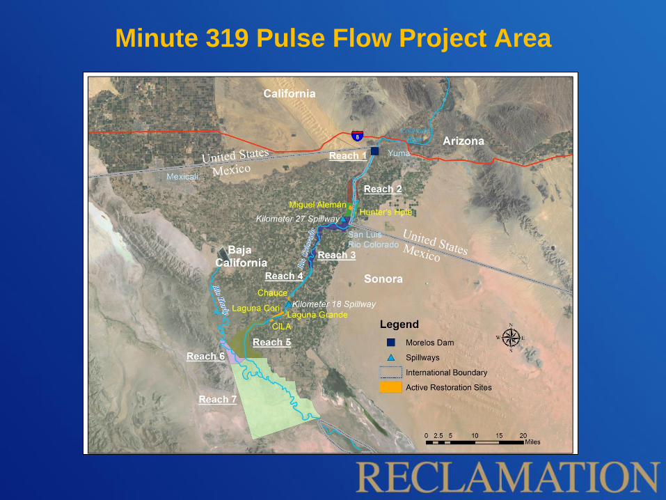
Minute 319 Pulse Flow Project Area

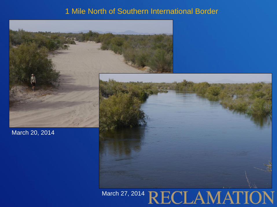
1 Mile North of Southern International Border

March 20, 2014

March 27, 2014

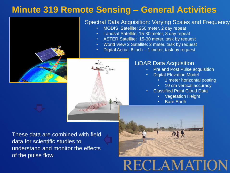
Minute 319 Remote Sensing – General Activities

LiDAR Data Acquisition • Pre and Post Pulse acquisition

• Digital Elevation Model:

• 1 meter horizontal posting

• 10 cm vertical accuracy

• Classified Point Cloud Data

• Vegetation Height

• Bare Earth

Spectral Data Acquisition: Varying Scales and Frequency • MODIS Satellite: 250 meter, 2 day repeat

• Landsat Satellite: 15-30 meter, 8 day repeat

• ASTER Satellite: 15-30 meter, task by request

• World View 2 Satellite: 2 meter, task by request

• Digital Aerial: 6 inch – 1 meter, task by request

These data are combined with field

data for scientific studies to

understand and monitor the effects

of the pulse flow

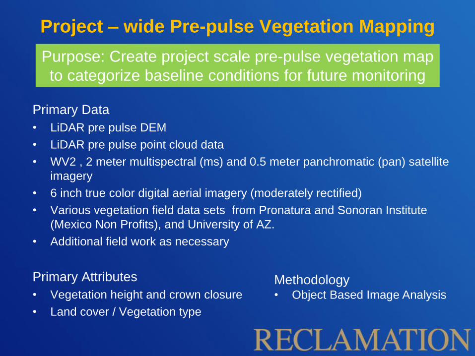
Project – wide Pre-pulse Vegetation Mapping

Primary Data

• LiDAR pre pulse DEM

• LiDAR pre pulse point cloud data

• WV2 , 2 meter multispectral (ms) and 0.5 meter panchromatic (pan) satellite

imagery

• 6 inch true color digital aerial imagery (moderately rectified)

• Various vegetation field data sets from Pronatura and Sonoran Institute

(Mexico Non Profits), and University of AZ.

• Additional field work as necessary

Primary Attributes

• Vegetation height and crown closure

• Land cover / Vegetation type

Purpose: Create project scale pre-pulse vegetation map

to categorize baseline conditions for future monitoring

Methodology • Object Based Image Analysis

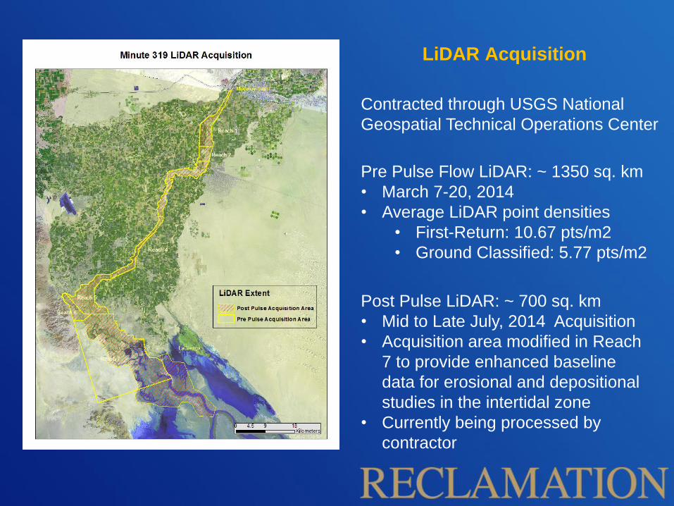
LiDAR Acquisition

Pre Pulse Flow LiDAR: ~ 1350 sq. km

• March 7-20, 2014

• Average LiDAR point densities

• First-Return: 10.67 pts/m2

• Ground Classified: 5.77 pts/m2

Post Pulse LiDAR: ~ 700 sq. km

• Mid to Late July, 2014 Acquisition

• Acquisition area modified in Reach

7 to provide enhanced baseline

data for erosional and depositional

studies in the intertidal zone

• Currently being processed by

contractor

Contracted through USGS National

Geospatial Technical Operations Center

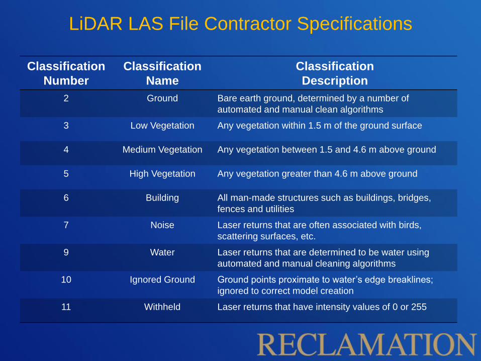
LiDAR LAS File Contractor Specifications

Classification

Number

Classification

Name

Classification

Description

2 Ground Bare earth ground, determined by a number of

automated and manual clean algorithms

3 Low Vegetation Any vegetation within 1.5 m of the ground surface

4 Medium Vegetation Any vegetation between 1.5 and 4.6 m above ground

5 High Vegetation Any vegetation greater than 4.6 m above ground

6 Building All man-made structures such as buildings, bridges,

fences and utilities

7 Noise Laser returns that are often associated with birds,

scattering surfaces, etc.

9 Water Laser returns that are determined to be water using

automated and manual cleaning algorithms

10 Ignored Ground Ground points proximate to water’s edge breaklines;

ignored to correct model creation

11 Withheld Laser returns that have intensity values of 0 or 255

World View 2 Imagery (WV2)

• WV2 multi-spectral / pan data collect requested through

National Geospatial-Intelligence Agency - NGA / US Geological

Survey Commercial Remote Sensing Space Policy (CRSSP, 2003).

• Imagery collected in Fall 2013 (pre-pulse flow)

• Unfortunately, a single collection date did not cover the

entire project area.

• However, most individual river reaches were covered by

a single image date.

• Imagery was mosaiced by reach to accommodate

varying image collection dates and image classification

and processing considerations.

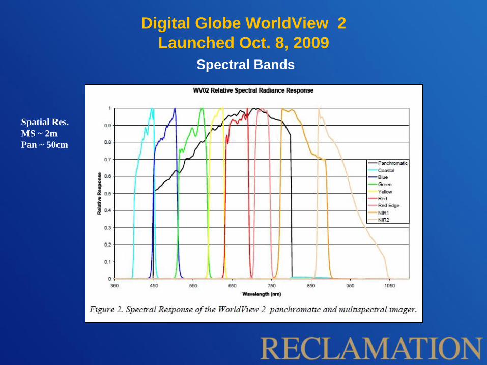
Digital Globe WorldView 2

Launched Oct. 8, 2009

Spectral Bands

Spatial Res.

MS ~ 2m

Pan ~ 50cm

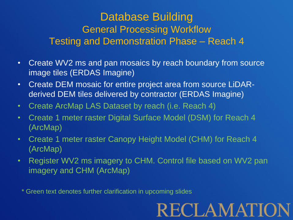
Database Building General Processing Workflow

Testing and Demonstration Phase – Reach 4

• Create WV2 ms and pan mosaics by reach boundary from source

image tiles (ERDAS Imagine)

• Create DEM mosaic for entire project area from source LiDAR-

derived DEM tiles delivered by contractor (ERDAS Imagine)

• Create ArcMap LAS Dataset by reach (i.e. Reach 4)

• Create 1 meter raster Digital Surface Model (DSM) for Reach 4

(ArcMap)

• Create 1 meter raster Canopy Height Model (CHM) for Reach 4

(ArcMap)

• Register WV2 ms imagery to CHM. Control file based on WV2 pan

imagery and CHM (ArcMap)

* Green text denotes further clarification in upcoming slides

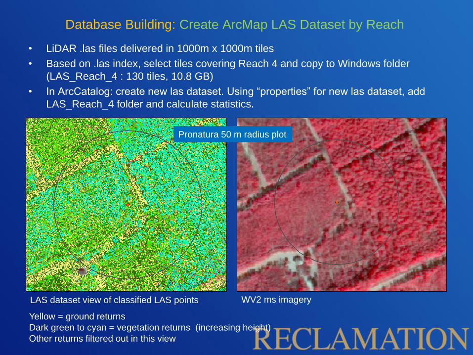
Database Building: Create ArcMap LAS Dataset by Reach

• LiDAR .las files delivered in 1000m x 1000m tiles

• Based on .las index, select tiles covering Reach 4 and copy to Windows folder

(LAS_Reach_4 : 130 tiles, 10.8 GB)

• In ArcCatalog: create new las dataset. Using “properties” for new las dataset, add

LAS_Reach_4 folder and calculate statistics.

LAS dataset view of classified LAS points WV2 ms imagery

Yellow = ground returns

Dark green to cyan = vegetation returns (increasing height)

Other returns filtered out in this view

Pronatura 50 m radius plot

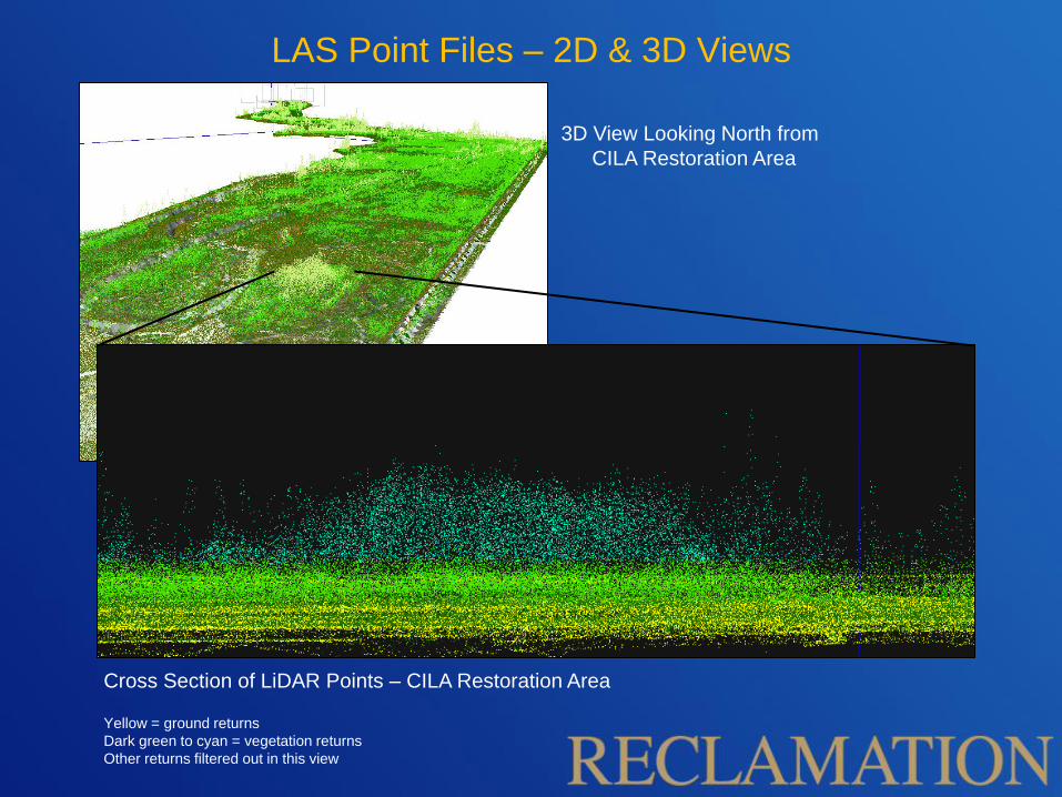
LAS Point Files – 2D & 3D Views

Yellow = ground returns

Dark green to cyan = vegetation returns

Other returns filtered out in this view

Cross Section of LiDAR Points – CILA Restoration Area

3D View Looking North from

CILA Restoration Area

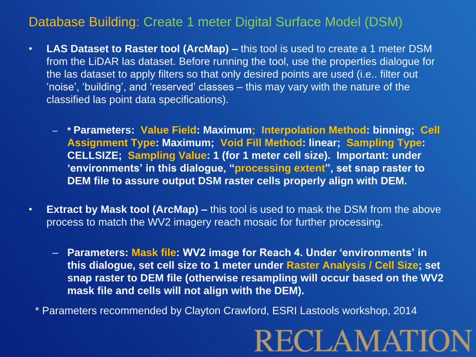
• LAS Dataset to Raster tool (ArcMap) – this tool is used to create a 1 meter DSM

from the LiDAR las dataset. Before running the tool, use the properties dialogue for

the las dataset to apply filters so that only desired points are used (i.e.. filter out

‘noise’, ‘building’, and ‘reserved’ classes – this may vary with the nature of the

classified las point data specifications).

– * Parameters: Value Field: Maximum; Interpolation Method: binning; Cell

Assignment Type: Maximum; Void Fill Method: linear; Sampling Type:

CELLSIZE; Sampling Value: 1 (for 1 meter cell size). Important: under

‘environments’ in this dialogue, “processing extent”, set snap raster to

DEM file to assure output DSM raster cells properly align with DEM.

• Extract by Mask tool (ArcMap) – this tool is used to mask the DSM from the above

process to match the WV2 imagery reach mosaic for further processing.

– Parameters: Mask file: WV2 image for Reach 4. Under ‘environments’ in

this dialogue, set cell size to 1 meter under Raster Analysis / Cell Size; set

snap raster to DEM file (otherwise resampling will occur based on the WV2

mask file and cells will not align with the DEM).

Database Building: Create 1 meter Digital Surface Model (DSM)

* Parameters recommended by Clayton Crawford, ESRI Lastools workshop, 2014

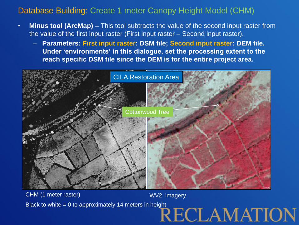
• Minus tool (ArcMap) – This tool subtracts the value of the second input raster from

the value of the first input raster (First input raster – Second input raster).

– Parameters: First input raster: DSM file; Second input raster: DEM file.

Under ‘environments’ in this dialogue, set the processing extent to the

reach specific DSM file since the DEM is for the entire project area.

Database Building: Create 1 meter Canopy Height Model (CHM)

CHM (1 meter raster) WV2 imagery

Black to white = 0 to approximately 14 meters in height

CILA Restoration Area

Cottonwood Tree

• Typical orthorectified image products do not have as high a level of

geometric control as that provided by LiDAR data. Imagery is

registered to the CHM before proceeding with classification work.

• ArcMap georeferencing tools are used to create transformation

control files based on tree centers; tying WV2 pan 0.5 imagery to

the CHM. This control file is then used to transform the WV2 pan

imagery, as well as WV2 ms imagery.

• ‘Adjust’ transformation in ArcMap is used, rather than a 3rd order

polynomial, as this method uses a combination of polynomial and

TIN interpolation to accommodate local variation, such as that seen

in areas of very tall trees.

• Na Li, et. al. Registration of Aerial Imagery and Lidar Data in Desert Areas Using the Centroids of

Bushes, PE&RS, August, 2013.

Database Building: Register WV2 ms imagery to CHM based on WV2

pan imagery and CHM for control (ArcMap)

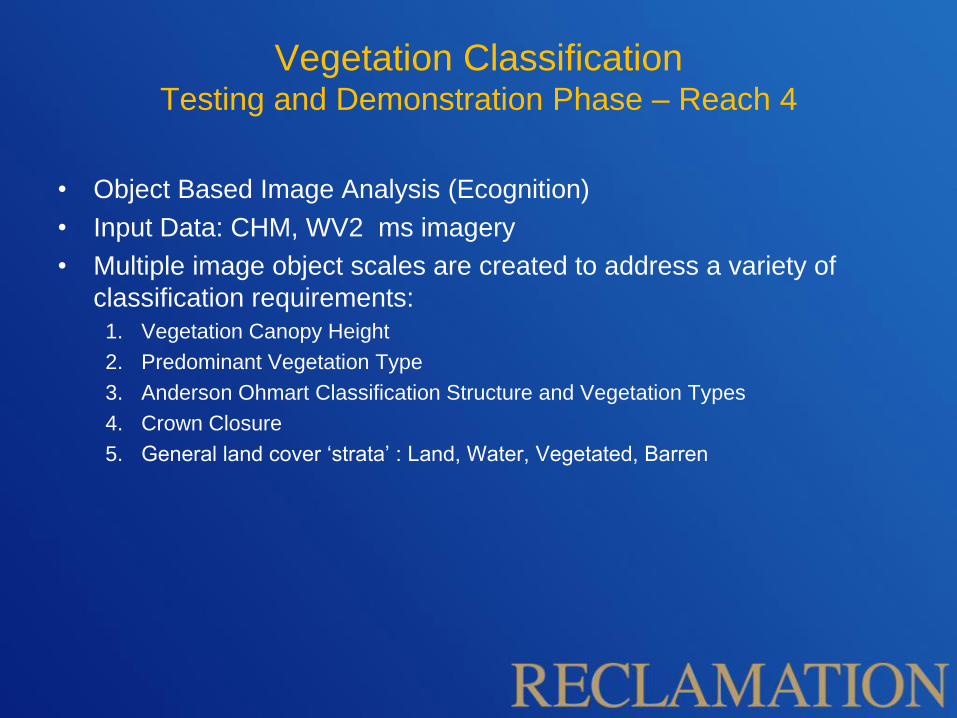
• Object Based Image Analysis (Ecognition)

• Input Data: CHM, WV2 ms imagery

• Multiple image object scales are created to address a variety of

classification requirements:

1. Vegetation Canopy Height

2. Predominant Vegetation Type

3. Anderson Ohmart Classification Structure and Vegetation Types

4. Crown Closure

5. General land cover ‘strata’ : Land, Water, Vegetated, Barren

Vegetation Classification Testing and Demonstration Phase – Reach 4

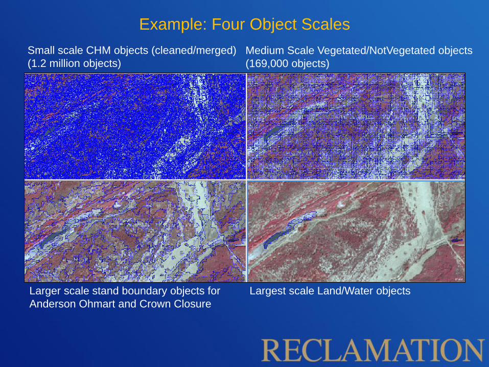
Example: Four Object Scales

Small scale CHM objects (cleaned/merged)

(1.2 million objects)

Medium Scale Vegetated/NotVegetated objects

(169,000 objects)

Largest scale Land/Water objects Larger scale stand boundary objects for

Anderson Ohmart and Crown Closure

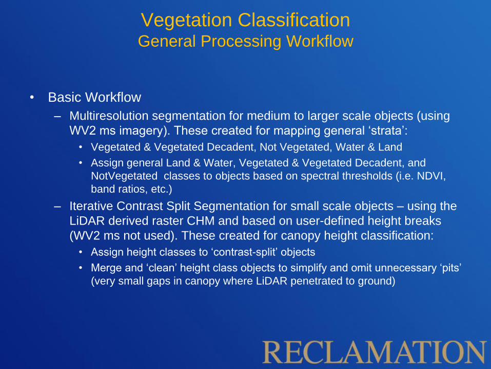
• Basic Workflow

– Multiresolution segmentation for medium to larger scale objects (using

WV2 ms imagery). These created for mapping general ‘strata’:

• Vegetated & Vegetated Decadent, Not Vegetated, Water & Land

• Assign general Land & Water, Vegetated & Vegetated Decadent, and

NotVegetated classes to objects based on spectral thresholds (i.e. NDVI,

band ratios, etc.)

– Iterative Contrast Split Segmentation for small scale objects – using the

LiDAR derived raster CHM and based on user-defined height breaks

(WV2 ms not used). These created for canopy height classification:

• Assign height classes to ‘contrast-split’ objects

• Merge and ‘clean’ height class objects to simplify and omit unnecessary ‘pits’

(very small gaps in canopy where LiDAR penetrated to ground)

Vegetation Classification General Processing Workflow

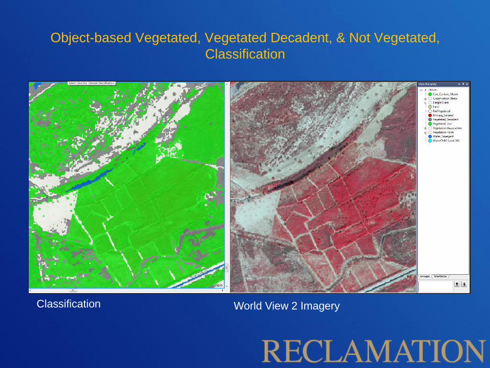
Object-based Vegetated, Vegetated Decadent, & Not Vegetated,

Classification

Classification World View 2 Imagery

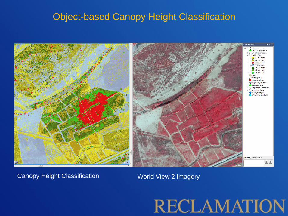
Object-based Canopy Height Classification

Canopy Height Classification World View 2 Imagery

• Basic Workflow

– Vegetation Type classification using fine scale CHM-objects

• Separate classifications within each height strata (reduces spectral variability

and class variability)

• Many potential object-based classification approaches including spectral

classifiers, decision tree classifiers, Boolean thresholds based on desired

variables.

• Many available variables including WV2 spectral bands and derived

variables (i.e.. NDVI, band ratios, texture, etc.), CHM metrics

– Multiresolution segmentation for vegetation stand-scale objects (using

WV2 ms imagery and raster CHM, and ‘built’ from fine scale CHM-

objects)

• Appropriate scale for assigning crown closure classes & vegetation classes

(based on specific classification system rules and the classification results at

the finer scale), and structure classes based on finer-scale CHM-objects.

General Processing Workflow: Vegetation Classification - Continued

Object-based Vegetation Type Classification – Fine Scale

Minimum Distance Classifier - Classified by height strata

- Variables used: WV2 multispectral bands

and various band ratios

World View 2 Imagery

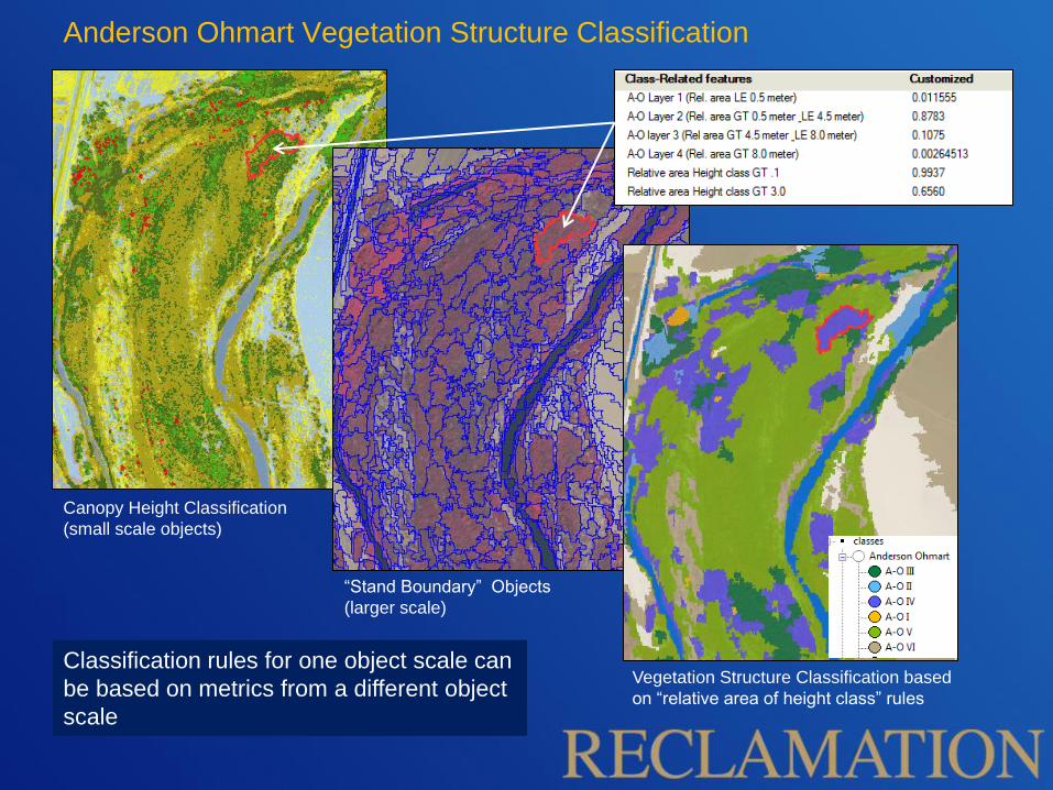
Anderson Ohmart Vegetation Structure Classification

Canopy Height Classification

(small scale objects)

“Stand Boundary” Objects

(larger scale)

Vegetation Structure Classification based

on “relative area of height class” rules

Classification rules for one object scale can

be based on metrics from a different object

scale

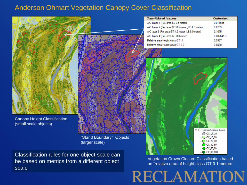
Anderson Ohmart Vegetation Canopy Cover Classification

Canopy Height Classification

(small scale objects)

“Stand Boundary” Objects

(larger scale)

Vegetation Crown Closure Classification based

on “relative area of height class GT 0.1 meters

Classification rules for one object scale can

be based on metrics from a different object

scale

Thank You !

Jeff Milliken, Colorado River Delta, Mexico

Additional Resources

• Video on contrast split segmentation for developing Object-Based CHM:

http://www.uvm.edu/~joneildu/Video/Definiens/TreeCanopy_LiDAR/TreeCanopy_LiDAR_controller.swf

Jarlath O’Neil-Dunne , Univ. of Vermont, Director Geospatial Analysis Center

• Ecognition video library on OBIA and LiDAR – examples • (search Ecognition tutorial in Google or go to Ecognition website)

• Sesnie, Steven, Mueller, J. et. al., Landscape-scale habitat characterization for

the golden-cheeked warbler and black-capped vireo using LiDAR and NAIP-

CIR imagery at Balcones Canyonlands National Wildlife Refuge, TX

(unpublished ASPRS chapter presentation)

• Fagan and DeFries, Measurement and Monitoring of the World’s Forests,

A Review and Summary of Remote Sensing Technical Capability, 2009–2015

http://www.rff.org/RFF/Documents/RFF-Rpt-Measurement%20and%20Monitoring_Final.pdf