mit joint program on the science and policy of global … · the mit joint program on the science...
TRANSCRIPT

MIT Joint Program on theScience and Policy of Global Change
Analysis of Climate Policy Targetsunder Uncertainty
Mort Webster, Andrei P. Sokolov, John M. Reilly, Chris E. Forest, SergeyPaltsev, Adam Schlosser, Chien Wang, David Kicklighter, Marcus Sarofim,
Jerry Melillo, Ronald G. Prinn, and Henry D. Jacoby
Report No. 180September 2009
The MIT Joint Program on the Science and Policy of Global Change is an organization for research,independent policy analysis, and public education in global environmental change. It seeks to provide leadershipin understanding scientific, economic, and ecological aspects of this difficult issue, and combining them into policyassessments that serve the needs of ongoing national and international discussions. To this end, the Program bringstogether an interdisciplinary group from two established research centers at MIT: the Center for Global ChangeScience (CGCS) and the Center for Energy and Environmental Policy Research (CEEPR). These two centersbridge many key areas of the needed intellectual work, and additional essential areas are covered by other MITdepartments, by collaboration with the Ecosystems Center of the Marine Biology Laboratory (MBL) at Woods Hole,and by short- and long-term visitors to the Program. The Program involves sponsorship and active participation byindustry, government, and non-profit organizations.
To inform processes of policy development and implementation, climate change research needs to focus onimproving the prediction of those variables that are most relevant to economic, social, and environmental effects.In turn, the greenhouse gas and atmospheric aerosol assumptions underlying climate analysis need to be related tothe economic, technological, and political forces that drive emissions, and to the results of international agreementsand mitigation. Further, assessments of possible societal and ecosystem impacts, and analysis of mitigationstrategies, need to be based on realistic evaluation of the uncertainties of climate science.
This report is one of a series intended to communicate research results and improve public understanding of climateissues, thereby contributing to informed debate about the climate issue, the uncertainties, and the economic andsocial implications of policy alternatives. Titles in the Report Series to date are listed on the inside back cover.
Henry D. Jacoby and Ronald G. Prinn,Program Co-Directors
For more information, please contact the Joint Program OfficePostal Address: Joint Program on the Science and Policy of Global Change
77 Massachusetts AvenueMIT E19-411Cambridge MA 02139-4307 (USA)
Location: 400 Main Street, CambridgeBuilding E19, Room 411Massachusetts Institute of Technology
Access: Phone: +1(617) 253-7492Fax: +1(617) 253-9845E-mail: glo balcha nge @mi t .e duWeb site: ht t p://gl o balch ange .m i t .e du /
Printed on recycled paper

Analysis of Climate Policy Targets under Uncertainty
Mort Webster∗† #, Andrei P. Sokolov*, John M. Reilly*, Chris E. Forest&, Sergey Paltsev*,
Adam Schlosser*, Chien Wang*, David Kicklighter‡, Marcus Sarofim@, Jerry Melillo‡, Ronald G. Prinn*, Henry D. Jacoby*
Abstract
Although policymaking in response to the climate change is essentially a challenge of risk management, most studies of the relation of emissions targets to desired climate outcomes are either deterministic or subject to a limited representation of the underlying uncertainties. Monte Carlo simulation, applied to the MIT Integrated Global System Model (an integrated economic and earth system model of intermediate complexity), is used to analyze the uncertain outcomes that flow from a set of century-scale emissions targets developed originally for a study by the U.S. Climate Change Science Program. Results are shown for atmospheric concentrations, radiative forcing, sea ice cover and temperature change, along with estimates of the odds of achieving particular target levels, and for the global costs of the associated mitigation policy. Comparison with other studies of climate targets are presented as evidence of the value, in understanding the climate challenge, of more complete analysis of uncertainties in human emissions and climate system response.
Contents
1. INTRODUCTION .................................................................................................................... 2 2. ANALYSIS METHODS............................................................................................................4
2.1 Model Components ............................................................................................................4 2.2 Monte Carlo Simulation Design.........................................................................................5
2.2.1 Parameter Distributions ............................................................................................6 2.2.2 Sampling Design........................................................................................................8
2.3 Stabilization Scenarios .......................................................................................................9 3. RESULTS OF THE ANALYSIS.............................................................................................12
3.1 Uncertainty in Climate under Stabilization Scenarios......................................................12 3.1.1 Emissions .................................................................................................................12 3.1.2 Concentrations.........................................................................................................13 3.1.3 Radiative Forcing ....................................................................................................18 3.1.4 Temperature Change ...............................................................................................18 3.1.5 Sea Ice .....................................................................................................................22
3.2 Reduction of the Probability of Exceeding Targets or Critical Levels .............................26 3.3 Uncertainty in the Global Cost of Emissions Mitigation..................................................29
4. COMPARISON WITH OTHER STUDIES.............................................................................31 5. DISCUSSION..........................................................................................................................37 6. REFERENCES ........................................................................................................................40 APPENDIX..................................................................................................................................45
∗ Joint Program on the Science and Policy of Global Change, Massachusetts Institute of Technology,
Cambridge, MA. † Engineering Systems Division, Massachusetts Institute of Technology, Cambridge, MA. # Corresponding author (email: [email protected]). & Dept. of Meteorology, Pennsylvania State University, University Park, PA. ‡ The Ecosystems Center, Marine Biological Laboratory, Woods Hole, MA. @ AAAS Science and Technology Policy Fellow, U.S. Environmental Protection Agency.
1

1. INTRODUCTION The United Nations Framework Convention on Climate Change (FCCC) states its
objective as: “…stabilization of greenhouse gas concentrations in the atmosphere at a
level that would prevent dangerous anthropogenic interference with the climate system”
(UNFCCC, 1992), and discussion of such a long-term goal is a continuing focus of the
Working Group on Long-Term Cooperative Action under the Bali Action Plan (UN
FCCC, 2007). This framing of the task has led to a focus on the calculation of the total
emissions of CO2 (or of all greenhouse gases stated in CO2-equivalents) that can be
allowed over the century while maintaining a maximum atmospheric concentration.
In addition to objectives framed in terms of atmospheric concentrations, the climate
goal also has been stated as a maximum increase, from human influence, to be allowed in
global average temperature. For example, the European Union has adopted a limit of 2°C
above the pre-industrial level, and in 2009 this 2°C target received an endorsement, if not
a firm commitment, from the leaders of the G8 nations (G8 Summit, 2009).1 Because of
the uncertainty in the temperature change projected to be caused by any path of global
emissions, the policy goal is sometimes stated in terms of a maximum increase in
radiative forcing by long-lived greenhouse gases, stated in watts per square meter
(W/m2). For example, this last approach was taken by a study of stabilization targets
undertaken by the U.S. Climate Change Science Program (CCSP) (Clarke et al., 2007),
and a set of radiative forcing targets form the basis for construction of scenarios to be
used in the IPCC’s 5th Assessment Report (Moss et al., 2007).
Though the climate policy challenge is essentially one of risk management, requiring
an understanding of uncertainty, most analyses of the emissions implications of these
various policy targets have been deterministic, applying scenarios of emissions and
reference (or at best median) values of parameters that represent aspects of the climate
system response, and the cost of emissions control. Examples of these types of studies as
carried out by governmental bodies include the U.S. CCSP study mentioned above
(Clarke et al., 2007) which applied three integrated assessment models to the study of
four alternative stabilization levels, and the analysis of the cost of emissions targets in the
1 The G8 leaders that they, “recognized the scientific view on the need to keep global temperature rise
below 2 degrees above pre-industrial levels.”
2
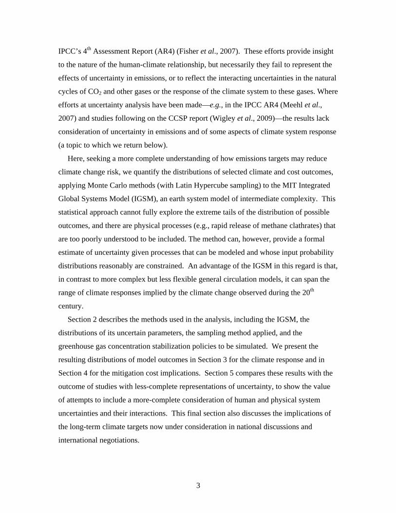
IPCC’s 4th Assessment Report (AR4) (Fisher et al., 2007). These efforts provide insight
to the nature of the human-climate relationship, but necessarily they fail to represent the
effects of uncertainty in emissions, or to reflect the interacting uncertainties in the natural
cycles of CO2 and other gases or the response of the climate system to these gases. Where
efforts at uncertainty analysis have been made—e.g., in the IPCC AR4 (Meehl et al.,
2007) and studies following on the CCSP report (Wigley et al., 2009)—the results lack
consideration of uncertainty in emissions and of some aspects of climate system response
(a topic to which we return below).
Here, seeking a more complete understanding of how emissions targets may reduce
climate change risk, we quantify the distributions of selected climate and cost outcomes,
applying Monte Carlo methods (with Latin Hypercube sampling) to the MIT Integrated
Global Systems Model (IGSM), an earth system model of intermediate complexity. This
statistical approach cannot fully explore the extreme tails of the distribution of possible
outcomes, and there are physical processes (e.g., rapid release of methane clathrates) that
are too poorly understood to be included. The method can, however, provide a formal
estimate of uncertainty given processes that can be modeled and whose input probability
distributions reasonably are constrained. An advantage of the IGSM in this regard is that,
in contrast to more complex but less flexible general circulation models, it can span the
range of climate responses implied by the climate change observed during the 20th
century.
Section 2 describes the methods used in the analysis, including the IGSM, the
distributions of its uncertain parameters, the sampling method applied, and the
greenhouse gas concentration stabilization policies to be simulated. We present the
resulting distributions of model outcomes in Section 3 for the climate response and in
Section 4 for the mitigation cost implications. Section 5 compares these results with the
outcome of studies with less-complete representations of uncertainty, to show the value
of attempts to include a more-complete consideration of human and physical system
uncertainties and their interactions. This final section also discusses the implications of
the long-term climate targets now under consideration in national discussions and
international negotiations.
3
2. ANALYSIS METHODS
2.1 Model Components The MIT Integrated Global System Model includes sub-models of the relevant parts of
the natural earth system and a model of human activity and emissions. Here we apply
Version 2 of the IGSM as described in Sokolov et al. (2005, 2009b). The model includes
the following components:
• A model of human activities and emissions, the Emissions Prediction and Policy
Analysis Model (Paltsev et al., 2005).
• An atmospheric dynamics, physics and chemistry model (Sokolov and Stone 1998;
Wang et al., 1998), which includes a sub-model of urban chemistry (Calbo et al.,
1998; Mayer et al., 2000; Prinn et al., 2007).
• A mixed-layer, anomaly-diffusing ocean model [ADOM] (Sokolov et al., 2005;
Sokolov et al., 2007), with carbon cycle and sea ice sub-models.
• A land system model (Schlosser et al., 2007) that combines the Terrestrial Ecosystem
Model [TEM] (Felzer et al., 2004; Sokolov et al., 2008), a Natural Emissions Model
[NEM] (Liu 1996), and the Community Land Model [CLM] (Bonan et al., 2002).
Together these components describe the global, terrestrial water, energy, and
biogeochemical budgets and terrestrial ecosystem processes that govern them.
The climate system component of the IGSM is a fully coupled model which enables
the simulation of feedbacks between components. The time steps in the various sub-
models range from 10 minutes for atmospheric dynamics to one month for certain
terrestrial processes, reflecting differences in the characteristic timescales of the
underlying natural phenomena.
The IGSM differs from similar models by its inclusion of significant chemical and
biological detail. In particular, natural fluxes of CO2, CH4 and N2O are estimated from
the simulated activities of plants and microbes on land and in the oceans; these vary over
the earth’s surface in response to vegetation distribution and simulated variations in light
availability as influenced by clouds and aerosols, climate, atmospheric chemistry (CO2
and O3), terrestrial hydrology, and oceanic acidity. The processes governing these natural
fluxes are coupled to the relevant climate, terrestrial hydrology, soil/vegetation, and
ocean processes to capture their dependence on temperature, rainfall, nutrient availability,
4

organic substrates, ocean acidity and other variables. Global anthropogenic emissions of
CO2, CO, NOx, volatile organic compounds (VOCs), black carbon (BC), SOx and other
key species are estimated by a regionally disaggregated model of global economic growth
(Paltsev et al., 2005). This procedure allows for treatment over time of a shifting mix and
geographical distribution of emissions.
Another feature of the IGSM for uncertainty analysis is its flexibility, allowing it to
reproduce the projections of a wide range of 3D Atmosphere-Ocean General Circulation
Models (AOGCMs). This aspect of the analysis is accomplished by varying cloud
feedback and deep-ocean mixing parameters (Sokolov et al., 2003; Forest et al., 2008).
Whereas the climate system response to external forcings, as represented in an AOGCM,
is a result of many parametric and structural formulations that are not easily varied, the
IGSM can simulate a wide and continuous range of climate response, permitting
parametric uncertainty analysis that would not be possible in the larger models.
2.2 Monte Carlo Simulation Design Monte Carlo simulation is a widely-used set of techniques for characterizing
uncertainty in numerical models resulting from uncertainty in model parameters (e.g.,
Rubenstein and Kroese, 2008). The basic steps in Monte Carlo analysis are: (1) identify
uncertain parameters and develop probability distributions for them, (2) sample from the
distributions to construct multiple sets of parameter values, and (3) simulate large
ensembles of model runs (hundreds or thousands of runs in each ensemble) using the
sampled parameter values. The distribution of model outcomes from the ensemble of
simulations provides estimates of future uncertainty, conditional on the model structure
and the distributions of uncertain parameters.
The results are also conditional on specific assumptions under which future scenarios
are constructed. As applied here, the no-policy results assume there are no direct efforts
to control emissions of long-lived greenhouse gases. Each of four emissions control
levels then creates a different estimate of uncertainty conditioned on achieving that policy
target. The ensemble size can also be an issue. With pure random sampling the ensemble
size required to obtain an estimate with suitable accuracy can be in the thousands to tens
of thousands of model simulations, making this approach infeasible even for models like
the IGSM that, although simplified, still require significant computer time. Fortunately,
5

the size of the required sample can be significantly reduced by applying well-designed
sampling strategies. Below, we describe the probability distributions assumed for the
model parameters, and the sampling strategy and ensemble size used in our calculations.
2.2.1 Parameter Distributions The details of the probability distributions developed for each model parameter, as
well as the data sources used in constructing each distribution, are documented by
Webster et al. (2008a) for the economic model parameters, and by both Forest et al.
(2008) and Sokolov et al. (2009b) for the earth system model. Here we briefly
summarize these uncertain parameters; their probability distributions are provided in
Appendix A.
For the economic (EPPA) model, with its sixteen regions with different characteristics,
probability distributions are constructed for over 100 separate socio-economic and
technological parameters. These parameters can be grouped into the following broad
categories:
• Elasticities of Substitution
• Labor Productivity Growth Rates
• Autonomous Energy Efficiency Improvement (AEEI)
• Fossil Fuel Resource Availability
• Population Growth
• Urban Pollutant Trends
• Future Energy Technologies
• Non-CO2 Greenhouse Gas Trends
• Capital Vintaging
The distributions for elasticities of substitution, labor productivity growth rates, AEEI,
fossil fuel resources, population growth, and urban air pollutant trends are based on
historical data and/or other published studies. The distributions for the cost of future
energy technologies, trends of non-CO2 greenhouse gas emissions, and capital vintaging
are based primarily on expert elicitations, documented in Webster et al. (2008a).
Taking advantage of the sensitivity of emissions to each parameter revealed in earlier
studies (Webster et al., 2002; Webster et al., 2003), we focus on improving the basis for
estimates of uncertainty in labor productivity growth rates, trends in urban air pollutant
6
emissions per unit of activity, and the elasticities of substitution. An effort was made to
base these estimates on observations as opposed to relying on expert elicitation as in our
earlier studies. Labor productivity growth rates, which are a primary driver of economic
growth in the model, are now based on observed GDP variability over the period 1950-
2000. The variability is used to sample future growth rates as a random walk with drift,
where the drift is the reference growth path of the EPPA model and the random walk
component is sampled for each 5-year period, producing more realistic growth paths
where regions experience periods of faster or slower growth. Previous work sampled high
or low growth rates that then were applied for the entire 100-year forecast horizon.
Future trends in urban pollutants, such as SO2 and NOx, are now based on the stochastic
emissions frontier analysis of 15 countries in Stern (2005, 2006), and so have a stronger
empirical foundation. For distributions for elasticities of substitution between different
inputs to production (e.g., capital vs. labor, capital/labor bundle vs. energy bundle) we
use estimates from published econometric studies.
The probability distributions for uncertain physical parameters in the earth system
model are described in Sokolov et al. (2009b). Five uncertain parameters are treated in
this study:
• Climate sensitivity
• Mixing of heat into the deep ocean
• Aerosol radiative forcing
• CO2 fertilization effect in terrestrial ecosystems
• Precipitation frequency trends as a function of increasing temperature.
The joint distribution of the first three uncertainties – climate sensitivity, ocean heat
uptake, and aerosol forcing – is constrained by 20th century observations (Forest et al.,
2008). Samples for these three parameters are drawn from their joint distribution in order
to capture the interdependence implied by observations. The probability distribution used
in this analysis is based on the estimates of the 20th century change in deep-ocean heat
content for the 0-3000m layer from Levitus et al. (2005). Other data analyses have been
prepared for the upper ocean (0-700m layer) (Domingues et al., 2008; Levitus et al.,
2009; Ishii and Kimoto, 2009), which would yield alternative joint distributions. These
more recent efforts differ from the earlier Levitus et al. (2005) in the application of bias
7
corrections to the various ocean temperature records. In addition, the change in ocean
heat content below 700m has not been estimated in these more recent data analyses and
so assumptions are required about the additional temperature change in the deep ocean.
Examples of the sensitivity of future climate projections to the choice of the deep ocean
temperature estimates, used to construct input distributions from climate parameters, are
given in Sokolov et al. (2009a, b).
We also include here two physical uncertainties not treated by Webster et al. (2003):
uncertainty in the CO2 fertilization effect on vegetation productivity, and the change in
the frequency of precipitation as a function of increases in surface temperature. The
former affects how much CO2 is removed from the atmosphere by vegetation and
potentially retained in plants and soils. The latter affects emissions of nitrous oxide from
soils as those emissions depend on periods of soil saturation. Uncertainty in the carbon
uptake by the ocean is not considered as an independent uncertainty but is linked to the
uncertainty in the oceanic heat uptake (see Sokolov et al., 2009b for details).
2.2.2 Sampling Design To limit the ensemble size, we employ stratified sampling (see Rubenstein and Kroese
2008, Ch. 5) and, in particular, the Latin Hypercube method for sampling across multiple
parameters (McKay et al., 1979). Numerical experiments demonstrate that, compared
with pure random sampling, the outcome distributions converge more quickly to the
limiting distributions as sample size increases. We use 400 samples in each ensemble, a
sample size that, for Latin Hypercube sampling, has been shown to approximate well the
limiting distribution for many nonlinear models2.
As noted previously, there is correlation among some of the input parameters. For the
physical climate parameters, correlation is modeled by sampling directly from the joint
distribution described in the previous section. For many of the economic parameters, we
impose correlation structure on related subsets of parameters (see Webster et al., 2008a 2 For the no policy scenario we tested the adequacy of the ensemble size by comparing sample sizes of 100,
200, 300, 400, 500, and 1000. To do this we performed 20 independent ensembles (drawing different sample sets for each) for each ensemble size, and compared the standard deviation of the estimate of median temperature change to the mean estimate of the standard deviation from the 20 ensembles. The standard deviation of the estimate of the median fell from 0.5% with 100 samples, to 0.2% with 400 samples, and had no appreciable improvement with 500 or 1000 samples. Similarly, the standard deviation of the estimate of the 0.95 fractile fell from 1.8% of its mean with 100 samples to 0.8% with 400 samples, and 0.75% with 1000 samples.
8

for details). The correlation is imposed during the sampling process using the procedure
from Iman and Conover (1982). This method chooses the next subinterval for sampling,
without replacement, by imposing the specified rank correlation.
Finally, to estimate the cost of a stabilization target, the simulated macroeconomic
consumption in a policy case is subtracted from that in the no-policy case. The procedure
involves pairwise comparisons of results for each policy case with that of the no-policy
case for each ensemble member, applying identical input values. The same 400 samples
are used for all five ensembles, with the only difference among them being the
introduction of different policy constraints.
2.3 Stabilization Scenarios We base the four stabilization scenarios on those developed, applying the MIT IGSM,
for the U.S. Climate Change Science Program (CCSP) Assessment Product 2.1A (Clarke
et al., 2007). These cases were designed to provide insight into discussions of climate
policy, particularly with regard to the implications of stabilization for emissions
trajectories, energy systems, and mitigation cost. We build on that exercise by performing
an uncertainty analysis of each of the CCSP policy constraints. The likelihoods of
different levels of climate change depend on the assumption that these emissions
scenarios are followed over the 100 year simulation horizon, and they are a best estimate
of that conditional future based on information we have today as represented by the
model structure and input uncertainty.3 Note that the IGSM simulation represents only
the potential human perturbation of the climate system, as departures from any natural
variability that may be experienced.
The stabilization scenarios in the CCSP exercise were labeled as Levels 1, 2, 3, and 4
(Clarke et al., 2007) and we retain those labels. Each of the emissions paths developed in
the MIT component of the CCSP exercise is applied as a vector of constraints on global
greenhouse gas emissions beginning in 2015. They are met in each simulated time period
and so allow the same cumulative emissions from 2015 to 2100. The quantity that is held 3 More will be learned as time passes policies can be expected to be revised over time as uncertainty is
reduced or we learn that median estimates are higher or lower. Nevertheless, analysis of what will happen if we follow a specific path through the horizon remain relevant to the decisions we must make today in the face of existing uncertainty. For studies that examine the implications of hypothetical future resolution of uncertainty see Webster et al. (2008b), Yohe et al. (2004), Kolstad (1996), and Ulph and Ulph (1997).
9

nearly constant under policy as parameters vary is the cumulative emissions of
greenhouse gases, as weighted by 100-year Global Warming Potentials (GWPs).4 When
these emissions levels are propagated through an earth system model with different
parameter values, the resulting concentrations will necessarily vary from these targets
because earth system feedbacks on concentrations are themselves uncertain and depend
on the realized climate.5
In Table 1, we describe the no-policy and four stabilization scenarios in terms of their
cumulative GWP-weighted emissions (denoted as CO2-equivalent (CO2-eq.) emissions)
over 2001-2100, which are 2.3, 3.4, 4.5, and 5.4 trillion (1012 or Tera) metric tons for
Levels 1, 2, 3, and 4, respectively. The no-policy scenario has median cumulative
emissions of 8.0 trillion metric tons. Table 1 also summarizes the ensemble results for
the median levels of
• CO2 concentrations,
• CO2-equivalent concentrations, calculated using radiative forcing due to long-
lived greenhouse gases only (they are listed in Table 2) relative to the pre-industrial
level,
• Change in total radiative forcing attributable to the long-lived greenhouse gases
and tropospheric ozone and aerosols, and
• Change in global mean surface temperature.
These calculated medians, stated in relation to the 1981-2009 average to be
comparable with results in the IPCC AR4, can help inform policy discussions by giving
some idea of the relations between emissions, concentrations and temperature increase.
4 Scenarios where there is low growth in emissions can lead to some ensemble members where emissions
are below the constraint level, especially for the Level 4 and Level 3 cases. The variation in GWP-weighted emissions is less than 1%.
5 Both the EPPA and earth system components of the IGSM have been updated since the CCSP study but these emissions scenarios remain of interest in terms of how our current best estimate of the cost of achieving them and their effectiveness in reducing the risk of serious climate change compares to the uncertainty in these estimates.
10

Table 1. Policy Constraints and Median Values of Key Results from Emissions Scenarios.
Policy Scenario
Cumulative Emissions
Constraints
Median Results for Each Ensemble Decadal Average for 2091-2100
(Changes Relative to 1981-2000 Average)
2001-2100
(Tt CO2-eq)1
CO2 Concen-trations (ppm)2
CO2–eq Concen-trations
Long-lived GHGs
(ppm)2
Change in
Radiative Forcing
(W/m2)3
Change in Annual Mean
Surface Temperature
(°C)3
Level 1 2.3 480 560 2.4 1.6
Level 2 3.4 560 660 3.5 2.3
Level 3 4.5 640 780 4.5 2.9
Level 4 5.4 710 890 5.3 3.4
No-Policy 8.04 870 1330 7.9 5.1 1Calculated using 100-year GWPs as calculated in Ramaswamy, et al. (2001). Includes gases
listed in Table 2. 2 Rounded to nearest 10 ppm. 3 Difference between the average for the decade 2091-2100 and 1981-2000; from pre-
industrial to 1981-2000 the net forcing for the included substances is estimated to be 1.8 W/m2).
4 Ensemble medians.
Table 2. Cumulative ensemble median CO2-equivalent emissions1,2, 2001-2100.
CO2 Emis.
(Gt CO2-eq)
CH4 Emis.
(Gt CO2-eq)
N2O Emis.
(Gt CO2-eq)
HFCs Emis.
(Gt CO2-eq)
PFCs Emis.
(Gt CO2-eq)
SF6 Emis.
(Gt CO2-eq)
Level 1 1400 651 275 3.1 0.4 0.8
Level 2 2330 733 305 4.1 0.4 0.8
Level 3 3340 811 332 4.7 0.4 0.8
Level 4 4120 886 361 5.2 0.4 0.8
No-Policy
5890 1300 531 181 7.3 16.2
1Calculated using 100-year GWPs (Ramaswamy, et al., 2001). 2 Rounded to nearest 3 significant figures.
Table 2 shows the cumulative emissions of each of the long-lived greenhouse gases.
The IGSM represents the group of hydrofluorocarbons (HFCs) as HFC-134a and
perfluorocarbons (PFCs) as perfluoromethane (CF4). Other assumptions in constructing
the stabilization scenarios are provided in Clarke et al. (2007).
11

3. RESULTS OF THE ANALYSIS
3.1 Uncertainty in Climate under Stabilization Scenarios Following Sokolov et al. (2009b), which examined the uncertainty in climate
projections in the absence of climate policy, we report results as decadal averages, for
example using 2091-2100 to represent the end period of the simulation. The 21st century
change is then expressed as the difference from the average for the period 1981-2000.
The resulting distributions of outcomes are presented graphically as frequency
distributions of the ensemble results. For each quantity, we choose a bin size such that
roughly 50-80 bins are used, and then smooth the results over five-bin intervals. The
specific binsize is given in the caption for each figure. The vertical coordinates are
normalized so that the area under each distribution integrates to unity.
3.1.1 Emissions The uncertainty in greenhouse gas emissions under the five scenarios was described in
Webster et al. (2008a). Before describing the uncertainty in climate outcomes, we first
show the path of the median emissions over time and the 5% and 95% bounds on
emissions for total greenhouse gas emissions in CO2-eq. from that study (Figure 1). The
no-policy case (black lines) has a large uncertainty range, while the policy cases do not
exhibit uncertainty, because the emissions constraint is binding – i.e., for the four
constraint cases the three lines are on top of one another because of this lack of
uncertainty in total emissions. (In fact, there is some uncertainty, too small to be seen in
the figure, in the initial year of the Level 4 and Level 3 scenarios, because under the low-
growth ensemble members the constraint is not binding.) There is some uncertainty in
the emissions of individual greenhouse gases, such as CO2 or CH4, because of variation
in the relative costs of abatement of the different gases and trading among greenhouse
gases is allowed using GWPs (see Webster et al., 2008a).
12

2000 2020 2040 2060 2080 2100
Glo
bal G
reen
hous
e G
as E
mis
sion
s(B
illion
Met
ric T
ons
CO
2-eq
)
0
20
40
60
80
100
120
140
160
180
No PolicyLevel 4Level 3Level 2Level 1
Figure 1. Global anthropogenic greenhouse gas emissions in CO2-eq in billion metric tons per year over 2000-2100. Solid lines indicate median emissions, and dashed lines indicate 5% and 95% bounds on emissions. The policy scenario is indicated by the color of lines: no-policy (black), Level 4 (Red), Level 3 (Orange), Level 2 (Blue), and Level 1 (Green).
3.1.2 Concentrations In Figure 2, we show the uncertainty in concentrations of the main long-lived
greenhouse gases averaged for the decade 2091-2100, expressed as frequency
distributions. Naturally, CO2, CH4, and N2O concentrations have a smaller variance in the
stabilization cases than under a no-policy assumption: the policy ensembles implement an
absolute constraint on emissions, so almost all emissions uncertainty has been eliminated
(see Figure 1). The main source of uncertainty in CO2 concentrations in simulations
under emissions constraint is the rate of carbon uptake by the ocean and terrestrial
ecosystems.6
The 95% bounds (0.025 to 0.975 fractile range) of the modeled CO2 concentrations
(Figure 2a) for the no-policy case are 691 – 1138 ppm (a difference of 447 ppm). In 6 As noted above, the IGSM considers uncertainty in carbon uptake by both ocean and terrestrial
vegetation. The IGSM accounts for the effect of nitrogen limitation on terrestrial carbon uptake, this significantly reduces both strength of feedback between climate and carbon cycle and uncertainty in this feedback (Sokolov et al., 2008).
13
simulations applying median no-policy emissions they are 777 and 932 ppm (155 ppm)
respectively (which gives an indication of the relative contribution of emissions and
earth-system uncertainty). The stabilization policies reduce these concentrations to 95%
bounds of 640 – 771 ppm for Level 4 controls (a 131 ppm difference), 580– 696 ppm for
Level 3 (a 116 ppm difference), 506 – 597 ppm for Level 2 (a 91 ppm difference), and
442 – 511 ppm for Level 1 (a 69 ppm difference). One implication of these results is that
emissions targets intended to achieve specific stabilization goals would need to be
adjusted over time as the uncertainty in the carbon cycle is resolved.
In the CCSP exercise (Clarke et al., 2007) the targets were designed to achieve
radiative forcing levels and, given the earth system parameters in the version of the MIT
IGSM used there, they also were consistent with ultimate stabilization of CO2 at 750,
650, 550, and 450 ppm. For all but the tightest Level 1 control case, actual stabilization
is modeled to occur after the 2100 horizon of the exercise and so concentrations in 2100
as simulated by the IGSM in the CCSP exercise were 677, 614, 526, and 451 ppm in the
Level 4 to Level 1 control cases, respectively. The median concentrations for the last
decade (2091-2100) in the ensembles developed here are 714, 643, 554, and 477 ppm in
the Level 4 to Level 1 in these same cases. The difference in CO2 concentration levels is
due primarily to changes in the parameterization of the carbon uptake by the deep ocean
between the two IGSM versions, which leads to lower carbon uptake in the version of the
model applied here, as explained in Sokolov et al. (2007).
For CH4 (Figure 2b) and N2O (Figure 2c), there is also still some uncertainty under
the stabilization cases due to the natural emissions of these gases, which depend in turn
on temperature and precipitation. Surface temperature influences microbial metabolism,
and therefore variations in estimated temperature among ensemble members will result in
variations in the estimated rates of methanogenesis and denitrification and the
corresponding natural emissions of CH4 and N2O, respectively. In addition, the intensity
and frequency of precipitation influences the formation of anaerobic zones within the soil
where denitrification occurs (Schlosser et al., 2007). Hence, variations in precipitation
will alter the extent and duration of these soil anaerobic zones and influence
denitrification rates, contributing to additional uncertainty in natural N2O emissions.
14

CO2 Concentrations (ppmv) for (2091-2100) - (1981-2000)400 600 800 1000 1200
Prob
abilit
y D
ensi
ty
0.0000.0020.0040.0060.0080.0100.0120.0140.0160.018
No PolicyLevel 4Level 3Level 2Level 1
a)
CH4 Concentrations (ppm) for (2091-2100) - (1981-2000)2 3 4 5 6
Prob
abilit
y D
ensi
ty
0
1
2
3
4
5
6No PolicyLevel 4Level 3Level 2Level 1
b)
N2O Concentrations (ppb) for (2091-2100) - (1981-2000)
360 380 400 420 440 460 480 500
Prob
abilit
y D
ensi
ty
0.00
0.02
0.04
0.06
0.08
0.10
0.12
0.14
0.16
No PolicyLevel 4Level 3Level 2Level 1
c)
Figure 2. Frequency distributions of concentrations averaged for the decade 2091-2100 for (a) CO2, (b) CH4, and (c) N2O. Frequency distributions calculated using bins of 1.0 ppm/ppb intervals, and smoothed over five bin interval. Horizontal lines show 5% to 95% interval, and vertical line indicates median.
15
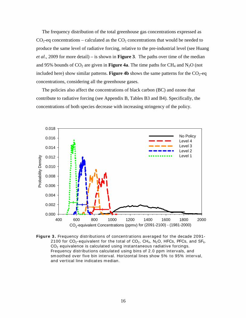
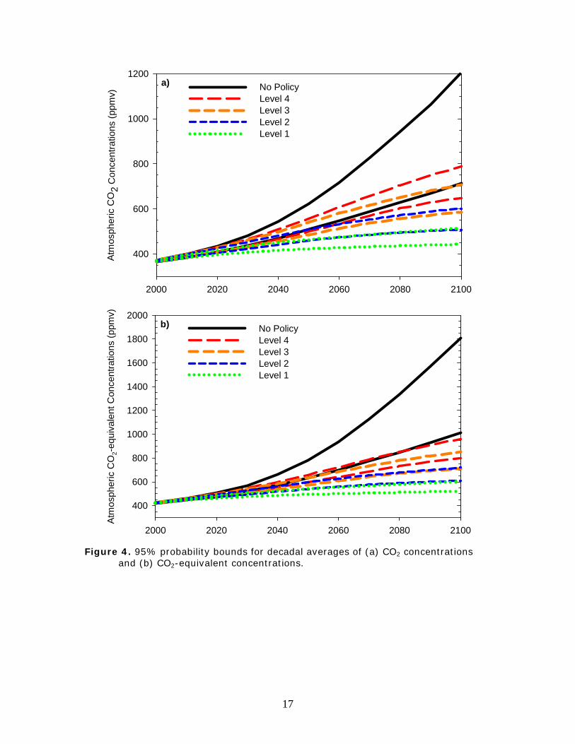
The frequency distribution of the total greenhouse gas concentrations expressed as
CO2-eq concentrations – calculated as the CO2 concentrations that would be needed to
produce the same level of radiative forcing, relative to the pre-industrial level (see Huang
et al., 2009 for more detail) – is shown in Figure 3. The paths over time of the median
and 95% bounds of CO2 are given in Figure 4a. The time paths for CH4 and N2O (not
included here) show similar patterns. Figure 4b shows the same patterns for the CO2-eq
concentrations, considering all the greenhouse gases.
The policies also affect the concentrations of black carbon (BC) and ozone that
contribute to radiative forcing (see Appendix B, Tables B3 and B4). Specifically, the
concentrations of both species decrease with increasing stringency of the policy.
CO2-equivalent Concentrations (ppmv) for (2091-2100) - (1981-2000)400 600 800 1000 1200 1400 1600 1800 2000
Prob
abilit
y D
ensi
ty
0.000
0.002
0.004
0.006
0.008
0.010
0.012
0.014
0.016
0.018
No PolicyLevel 4Level 3Level 2Level 1
Figure 3. Frequency distributions of concentrations averaged for the decade 2091-2100 for CO2-equivalent for the total of CO2, CH4, N2O, HFCs, PFCs, and SF6. CO2 equivalence is calculated using instantaneous radiative forcings. Frequency distributions calculated using bins of 2.0 ppm intervals, and smoothed over five bin interval. Horizontal lines show 5% to 95% interval, and vertical line indicates median.
16
2000 2020 2040 2060 2080 2100
Atm
osph
eric
CO
2 C
once
ntra
tions
(ppm
v)
400
600
800
1000
1200No PolicyLevel 4Level 3Level 2Level 1
a)
2000 2020 2040 2060 2080 2100
Atm
osph
eric
CO
2-eq
uiva
lent
Con
cent
ratio
ns (p
pmv)
400
600
800
1000
1200
1400
1600
1800
2000No PolicyLevel 4Level 3Level 2Level 1
b)
Figure 4. 95% probability bounds for decadal averages of (a) CO2 concentrations and (b) CO2-equivalent concentrations.
17
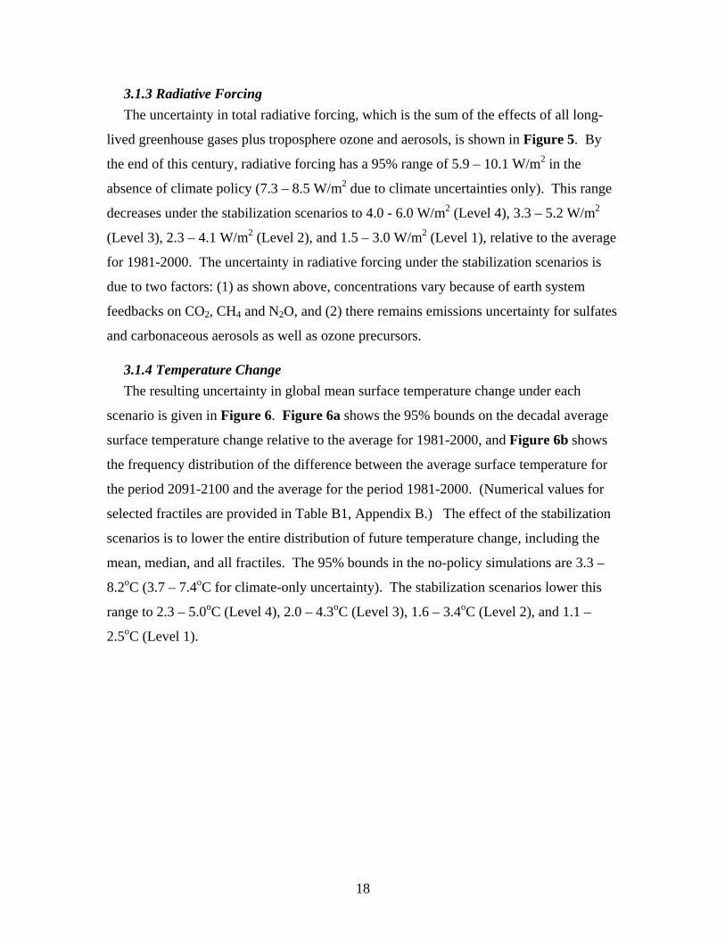
3.1.3 Radiative Forcing The uncertainty in total radiative forcing, which is the sum of the effects of all long-
lived greenhouse gases plus troposphere ozone and aerosols, is shown in Figure 5. By
the end of this century, radiative forcing has a 95% range of 5.9 – 10.1 W/m2 in the
absence of climate policy (7.3 – 8.5 W/m2 due to climate uncertainties only). This range
decreases under the stabilization scenarios to 4.0 - 6.0 W/m2 (Level 4), 3.3 – 5.2 W/m2
(Level 3), 2.3 – 4.1 W/m2 (Level 2), and 1.5 – 3.0 W/m2 (Level 1), relative to the average
for 1981-2000. The uncertainty in radiative forcing under the stabilization scenarios is
due to two factors: (1) as shown above, concentrations vary because of earth system
feedbacks on CO2, CH4 and N2O, and (2) there remains emissions uncertainty for sulfates
and carbonaceous aerosols as well as ozone precursors.
3.1.4 Temperature Change The resulting uncertainty in global mean surface temperature change under each
scenario is given in Figure 6. Figure 6a shows the 95% bounds on the decadal average
surface temperature change relative to the average for 1981-2000, and Figure 6b shows
the frequency distribution of the difference between the average surface temperature for
the period 2091-2100 and the average for the period 1981-2000. (Numerical values for
selected fractiles are provided in Table B1, Appendix B.) The effect of the stabilization
scenarios is to lower the entire distribution of future temperature change, including the
mean, median, and all fractiles. The 95% bounds in the no-policy simulations are 3.3 –
8.2oC (3.7 – 7.4oC for climate-only uncertainty). The stabilization scenarios lower this
range to 2.3 – 5.0oC (Level 4), 2.0 – 4.3oC (Level 3), 1.6 – 3.4oC (Level 2), and 1.1 –
2.5oC (Level 1).
18

2000 2020 2040 2060 2080 2100
Tota
l Rad
iativ
e Fo
rcin
g (w
/m2 )
0
2
4
6
8
10
12No PolicyLevel 4Level 3Level 2Level 1
a)
Total Radiative Forcing (w/m2)0 2 4 6 8 10 12
Prob
abilit
y D
ensi
ty
0.0
0.2
0.4
0.6
0.8
1.0
1.2
1.4
No PolicyLevel 4Level 3Level 2Level 1
b)
Figure 5. Total radiative forcing relative to 1981-2000 (greenhouse gases and aerosols) from all emissions for each policy case, shown as (a) 95% probability bounds over time, and (b) frequency distributions averaged for the decade 2091-2100. Frequency distributions calculated using bins of 0.1 w/m2 intervals, and smoothed over a five bin interval. Horizontal lines show 5% to 95% interval, and vertical line indicates median.
19

2000 2020 2040 2060 2080 2100
Dec
adal
Ave
rage
Glo
bal M
ean
Surfa
ce T
empe
ratu
re C
hang
e(2
091-
2100
) - (1
981-
2000
)
0
2
4
6
8
10No PolicyLevel 4Level 3Level 2Level 1
a)
Decadal Average Global Mean Surface Temperature Change(2091-2100) - (1981-2000)
0 2 4 6 8 10
Prob
abilit
y D
ensi
ty
0.0
0.2
0.4
0.6
0.8
1.0
1.2
1.4
No PolicyLevel 4Level 3Level 2Level 1
b)
Figure 6. Decadal average global mean temperature change shown as (a) 95% bounds over time relative to average for 1981-2000, and (b) frequency distributions of temperature change between the 1981-2000 average and the 2091-2100 average. Frequency distributions calculated using bins of 0.1 degree intervals, and smoothed over a five bin interval. Horizontal lines in b) show 5% to 95% interval, and vertical line indicates median.
20
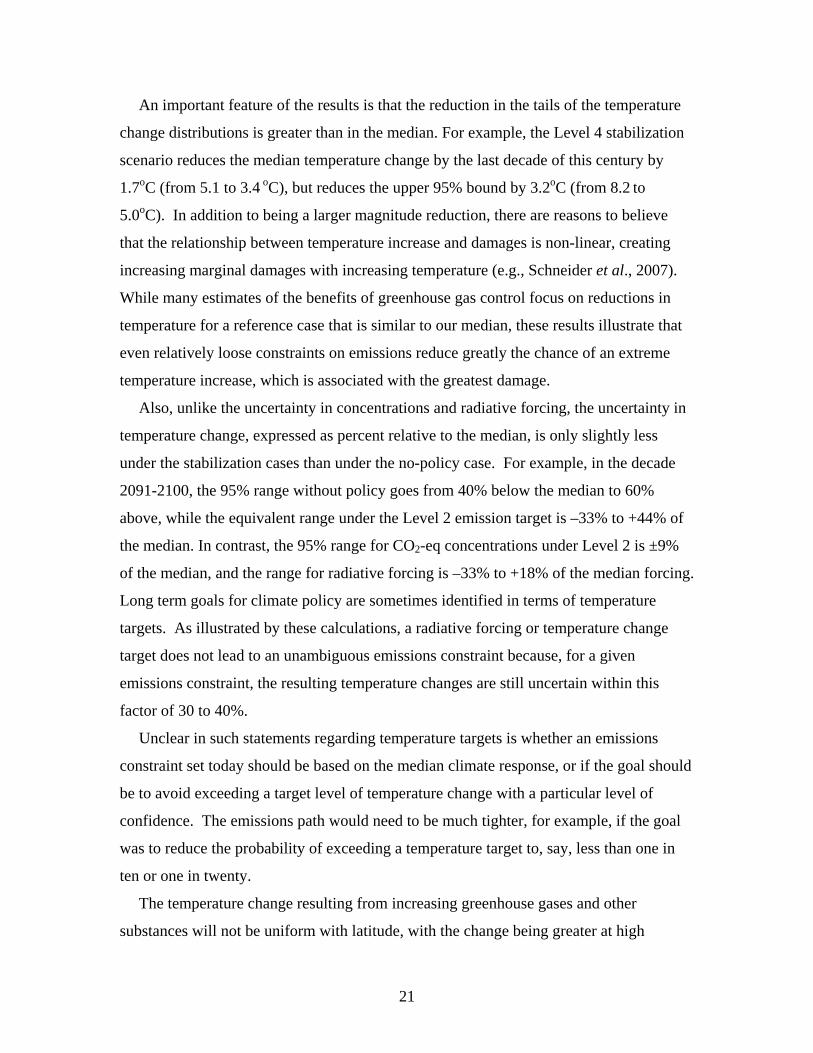
An important feature of the results is that the reduction in the tails of the temperature
change distributions is greater than in the median. For example, the Level 4 stabilization
scenario reduces the median temperature change by the last decade of this century by
1.7oC (from 5.1 to 3.4 oC), but reduces the upper 95% bound by 3.2oC (from 8.2 to
5.0oC). In addition to being a larger magnitude reduction, there are reasons to believe
that the relationship between temperature increase and damages is non-linear, creating
increasing marginal damages with increasing temperature (e.g., Schneider et al., 2007).
While many estimates of the benefits of greenhouse gas control focus on reductions in
temperature for a reference case that is similar to our median, these results illustrate that
even relatively loose constraints on emissions reduce greatly the chance of an extreme
temperature increase, which is associated with the greatest damage.
Also, unlike the uncertainty in concentrations and radiative forcing, the uncertainty in
temperature change, expressed as percent relative to the median, is only slightly less
under the stabilization cases than under the no-policy case. For example, in the decade
2091-2100, the 95% range without policy goes from 40% below the median to 60%
above, while the equivalent range under the Level 2 emission target is –33% to +44% of
the median. In contrast, the 95% range for CO2-eq concentrations under Level 2 is ±9%
of the median, and the range for radiative forcing is –33% to +18% of the median forcing.
Long term goals for climate policy are sometimes identified in terms of temperature
targets. As illustrated by these calculations, a radiative forcing or temperature change
target does not lead to an unambiguous emissions constraint because, for a given
emissions constraint, the resulting temperature changes are still uncertain within this
factor of 30 to 40%.
Unclear in such statements regarding temperature targets is whether an emissions
constraint set today should be based on the median climate response, or if the goal should
be to avoid exceeding a target level of temperature change with a particular level of
confidence. The emissions path would need to be much tighter, for example, if the goal
was to reduce the probability of exceeding a temperature target to, say, less than one in
ten or one in twenty.
The temperature change resulting from increasing greenhouse gases and other
substances will not be uniform with latitude, with the change being greater at high
21
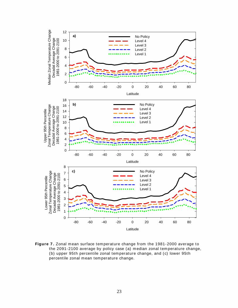
latitudes and lesser in the tropics (Meehl et al., 2007). Figure 7 shows our estimates of
the projected change in the zonal distribution of mean surface air temperature from the
1981-2000 average to the 2091-2100 average under each of the scenarios for the median
(Figure 7a), the upper 95% bound (Figure 7b), and the lower 95% bound (Figure 7c).
As is the case for global temperature change the reduction due to stabilization in the
upper 95% bound is greater than the reduction in the median temperature change.
As an example of the impact on high latitude temperature changes, we show the
frequency distributions for 60oN–90oN (Figure 8). Numerical values for mean, standard
deviation, and selected fractiles are given in Table B3 in Appendix B for a range of zonal
bands. As can be seen from these results, climate policies have a larger effect on
temperature changes at high latitudes than on global mean surface warming. The Level 4
policy scenario, for example, would reduce surface temperatures in high latitude regions
by between 2 and 7oC relative to the no-policy case or a 40% decrease, compared to a
range of 1 to 3oC or a 30% decrease in global mean surface warming.
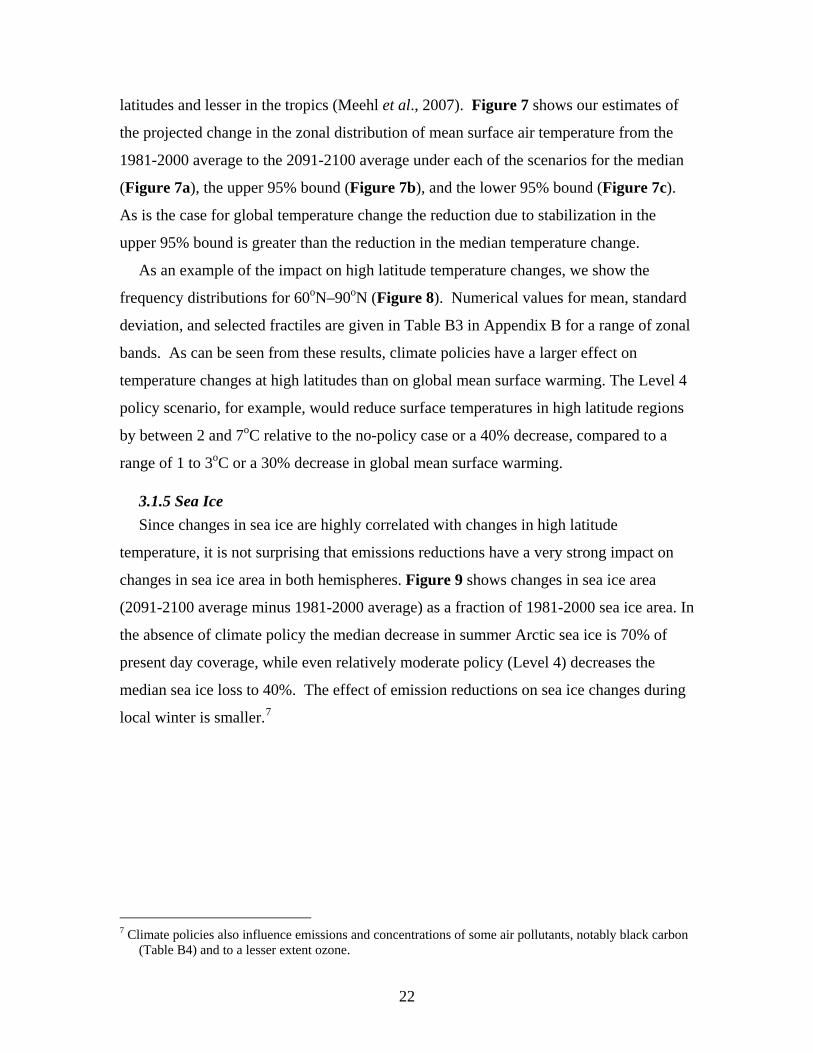
3.1.5 Sea Ice Since changes in sea ice are highly correlated with changes in high latitude
temperature, it is not surprising that emissions reductions have a very strong impact on
changes in sea ice area in both hemispheres. Figure 9 shows changes in sea ice area
(2091-2100 average minus 1981-2000 average) as a fraction of 1981-2000 sea ice area. In
the absence of climate policy the median decrease in summer Arctic sea ice is 70% of
present day coverage, while even relatively moderate policy (Level 4) decreases the
median sea ice loss to 40%. The effect of emission reductions on sea ice changes during
local winter is smaller.7
7 Climate policies also influence emissions and concentrations of some air pollutants, notably black carbon
(Table B4) and to a lesser extent ozone.
22
Latitude
-80 -60 -40 -20 0 20 40 60 80
Med
ian
Zona
l Tem
pera
ture
Cha
nge
Dec
adal
Ave
rage
Cha
nge
1981
-200
0 to
209
1-21
00
0
2
4
6
8
10
12No PolicyLevel 4Level 3Level 2Level 1
a)
Latitude
-80 -60 -40 -20 0 20 40 60 80
Upp
er 9
5th
Perc
entil
e Zo
nal T
empe
ratu
re C
hang
e D
ecad
al A
vera
ge C
hang
e 19
81-2
000
to 2
091-
2100
02468
1012141618
No PolicyLevel 4Level 3Level 2Level 1
b)
Latitude
-80 -60 -40 -20 0 20 40 60 80
Low
er 9
5th
Perc
entil
e Zo
nal T
empe
ratu
re C
hang
eD
ecad
al A
vera
ge C
hang
e 19
81-2
000
to 2
091-
2100
0
1
2
3
4
5
6
7
8No PolicyLevel 4Level 3Level 2Level 1
c)
Figure 7. Zonal mean surface temperature change from the 1981-2000 average to the 2091-2100 average by policy case (a) median zonal temperature change, (b) upper 95th percentile zonal temperature change, and (c) lower 95th percentile zonal mean temperature change.
23

Decadal Average Surface Temperature Change at 50o N(2091-2100) - (1981-2000)
0 2 4 6 8 10 12 14 16 18
Prob
abilit
y D
ensi
ty
0.0
0.2
0.4
0.6
0.8
1.0
No PolicyLevel 4Level 3Level 2Level 1
Figure 8. Frequency distributions for the decadal average surface temperature change at 60o-90oN between 1981-2000 and 2091-2100. Frequency distributions calculated using bins of 0.1 degree intervals, and smoothed over a five bin interval. Horizontal lines show 5% to 95% interval, and vertical line indicates median.
24

Fractional Change in Sea Ice - September, Northern HemisphereChange from 1981-2000 average to 2091-2100 Average
-1.0 -0.8 -0.6 -0.4 -0.2 0.0
Prob
abilit
y D
ensi
ty
0
2
4
6
8
10
12
14
16
18
No PolicyLevel 4Level 3Level 2Level 1
a)
Fractional Change in Sea Ice - March, Southern HemisphereChange from 1981-2000 average to 2091-2100 Average
-0.8 -0.6 -0.4 -0.2 0.0
Pro
babi
lity
Den
sity
0
5
10
15
20
25
30
No PolicyLevel 4Level 3Level 2Level 1
b)
Figure 9. Changes in sea ice area (2091-2100 relative to 1981-2000) as a fraction of 1981-2000 coverage for (a) Northern Hemisphere in September, and (b) Southern Hemisphere in March. Frequency distributions calculated using bins of 0.0025 intervals, and smoothed over a five bin interval. Horizontal lines show 5% to 95% interval, and vertical line indicates median.
25
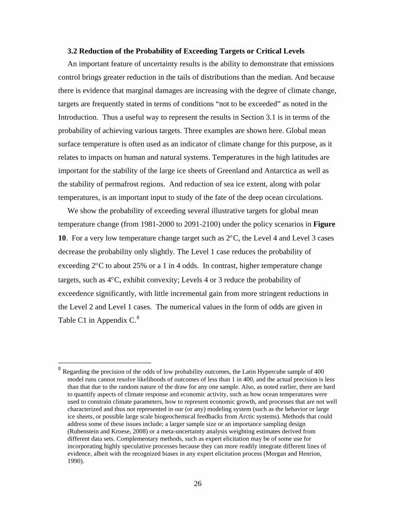
3.2 Reduction of the Probability of Exceeding Targets or Critical Levels An important feature of uncertainty results is the ability to demonstrate that emissions
control brings greater reduction in the tails of distributions than the median. And because
there is evidence that marginal damages are increasing with the degree of climate change,
targets are frequently stated in terms of conditions “not to be exceeded” as noted in the
Introduction. Thus a useful way to represent the results in Section 3.1 is in terms of the
probability of achieving various targets. Three examples are shown here. Global mean
surface temperature is often used as an indicator of climate change for this purpose, as it
relates to impacts on human and natural systems. Temperatures in the high latitudes are
important for the stability of the large ice sheets of Greenland and Antarctica as well as
the stability of permafrost regions. And reduction of sea ice extent, along with polar
temperatures, is an important input to study of the fate of the deep ocean circulations.
We show the probability of exceeding several illustrative targets for global mean
temperature change (from 1981-2000 to 2091-2100) under the policy scenarios in Figure
10. For a very low temperature change target such as 2°C, the Level 4 and Level 3 cases
decrease the probability only slightly. The Level 1 case reduces the probability of
exceeding 2°C to about 25% or a 1 in 4 odds. In contrast, higher temperature change
targets, such as 4°C, exhibit convexity; Levels 4 or 3 reduce the probability of
exceedence significantly, with little incremental gain from more stringent reductions in
the Level 2 and Level 1 cases. The numerical values in the form of odds are given in
Table C1 in Appendix C.8
8 Regarding the precision of the odds of low probability outcomes, the Latin Hypercube sample of 400
model runs cannot resolve likelihoods of outcomes of less than 1 in 400, and the actual precision is less than that due to the random nature of the draw for any one sample. Also, as noted earlier, there are hard to quantify aspects of climate response and economic activity, such as how ocean temperatures were used to constrain climate parameters, how to represent economic growth, and processes that are not well characterized and thus not represented in our (or any) modeling system (such as the behavior or large ice sheets, or possible large scale biogeochemical feedbacks from Arctic systems). Methods that could address some of these issues include; a larger sample size or an importance sampling design (Rubenstein and Kroese, 2008) or a meta-uncertainty analysis weighting estimates derived from different data sets. Complementary methods, such as expert elicitation may be of some use for incorporating highly speculative processes because they can more readily integrate different lines of evidence, albeit with the recognized biases in any expert elicitation process (Morgan and Henrion, 1990).
26
REF Level 4 Level 3 Level 2 Level 1
Pro
babi
lity
of E
xcee
ding
Illu
stra
tive
Glo
bal M
ean
Sur
face
Tem
pera
ture
Tar
get (
%)
0
20
40
60
80
1002 Degrees C3 Degrees C4 Degrees C5 Degrees C6 Degrees C
Figure 10. Change in the probability of exceeding illustrative targets for global mean surface temperature change, as measured by the change between the average for 1981-2000 and the average for 2091-2100. Lines indicate the change in probability under different policy cases for exceeding a given target: 2oC (green dotted line), 3oC (blue dashed line), 4oC (orange dashed line), 5oC (red dashed line), and 6oC (black solid line).
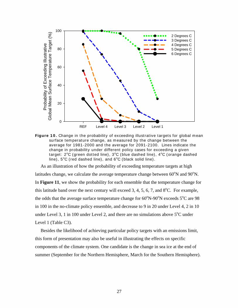
As an illustration of how the probability of exceeding temperature targets at high
latitudes change, we calculate the average temperature change between 60oN and 90oN.
In Figure 11, we show the probability for each ensemble that the temperature change for
this latitude band over the next century will exceed 3, 4, 5, 6, 7, and 8oC. For example,
the odds that the average surface temperature change for 60oN-90oN exceeds 5oC are 98
in 100 in the no-climate policy ensemble, and decrease to 9 in 20 under Level 4, 2 in 10
under Level 3, 1 in 100 under Level 2, and there are no simulations above 5oC under
Level 1 (Table C3).
Besides the likelihood of achieving particular policy targets with an emissions limit,
this form of presentation may also be useful in illustrating the effects on specific
components of the climate system. One candidate is the change in sea ice at the end of
summer (September for the Northern Hemisphere, March for the Southern Hemisphere).
27
REF Level 4 Level 3 Level 2 Level 1
Pro
babi
lity
of E
xcee
ding
Illu
stra
tive
Targ
et fo
rA
vera
ge S
urfa
ce T
empe
ratu
re C
hang
e 60
N-9
0N (%
)
0
20
40
60
80
100
3 Degrees C4 Degrees C5 Degrees C6 Degrees C7 Degrees C8 Degrees C
Figure 11. Change in the probability of exceeding illustrative targets for average
surface temperature change at 60oN to 90oN, as measured by the change between the average for 1981-2000 and the average for 2091-2100. Lines indicate the change in probability under different policy cases for exceeding a given target: 3oC (green dotted line), 4oC (blue dashed line), 5oC (orange dashed line), 6oC (red dashed line), 7oC (black solid line), and 8oC (brown dash-dot line).
28

REF Level 4 Level 3 Level 2 Level 1
Pro
babi
lity
(%) o
f Exc
eedi
ng
Illus
trativ
e Ta
rget
for C
hang
e in
Sea
Ice
Ext
ent
from
198
1-20
00 A
vera
geS
epte
mbe
r, N
orth
ern
Hem
isph
ere
0
20
40
60
80
100
ΔSea Ice < -20%ΔSea Ice < -30%ΔSea Ice < -40%ΔSea Ice < -50%ΔSea Ice < -60%
Figure 12. Change in the probability of exceeding illustrative targets for changes in
sea ice extent in September in the Northern Hemisphere relative to the average for 1981-2000. Lines indicate the change in probability under different policy cases for exceeding a given target: 20% decrease (green dotted line), 30% decrease (blue dashed line), 40% decrease (orange dashed line), 50% decrease (red dashed line), and 60% decrease (black solid line).
Figure 12 shows the probability from this analysis that the decrease in September
northern hemisphere sea ice cover from the 1981-2000 average to the 2091-2100 average
exceeds 20%, 30%, 40%, 50%, and 60%. For example, the odds of a decrease in sea ice
cover of more than 40% is 97 in 100 without climate policy, and falls to 2 in 5, 15 in 100,
1 in 100, and less than 1 in 400 under Levels 4, 3, 2, and 1, respectively (Table C4).
Similar odds are given in Table C5 for the Southern Hemisphere in March.
3.3 Uncertainty in the Global Cost of Emissions Mitigation The CCSP study of stabilization scenarios (Clarke et al., 2007) yielded, for each
participating model, a set of single estimates of the cost of achieving the atmospheric
targets, but of course the cost of achieving any global emissions target also is uncertain.
Monetized, global estimates of the cost of emissions mitigation over the century are
subject to many qualifications, discussed by Clarke et al. (2007), but nonetheless we
extend our illustration of the risk management framing of climate policy decisions by
29

No Poli
cy
Leve
l 4
Leve
l 3
Leve
l 2
Leve
l 1
Glo
bal C
onsu
mpt
ion
Loss
(%)
0
1
2
3
495% Probability Bounds50% Probability BoundsMedian
a)
No Poli
cy
Leve
l 4
Leve
l 3
Leve
l 2
Leve
l 1
Glo
bal C
onsu
mpt
ion
Loss
(%)
0
2
4
6
8
10
12
1495% Probability Bounds50% Probability BoundsMedian
b)
No Poli
cy
Leve
l 4
Leve
l 3
Leve
l 2
Leve
l 1
Glo
bal C
onsu
mpt
ion
Loss
(%)
0
5
10
15
20
2595% Probability Bounds50% Probability BoundsMedian
c)
Figure 13. Median, 50%, and 95% probability bounds of consumption loss (%) relative to no-policy case for the years (a) 2020, (b) 2060, and (c) 2100. Solid black line indicates median, dark grey shading indicates 50% probability interval, and light grey shading indicates 95% probability interval.
reproducing the results for uncertainty in the costs of emissions reductions as computed
by Webster et al. (2008a). As in Webster et al. (2008a) and Clarke et al. (2007), we use
the loss in global aggregate consumption as the measure of cost. Figure 13 shows the
uncertainty in the costs of abatement in 2020, 2050, and 2100 for the five scenarios. In
30

contrast to the probability of exceeding climate targets, which falls as the emissions cap
is tightened; the uncertainty in costs grows as the emissions cap is decreased.
4. COMPARISONS WITH OTHER STUDIES Formal uncertainty analysis of the type shown here is computationally demanding, and
as a result is infrequently conducted. Sometimes, however, assessments interpret the
range of outcomes across models as a proxy for the uncertainty range, or include
uncertainty in some but not all of the relevant processes. What is gained by the more
complete representation of uncertainty in this paper can be shown in a comparison of our
results with examples of other approaches.
One example is the CCSP study from which we drew the greenhouse gas constraints
used in the IGSM calculations performed for that study and adopted here. The IGSM
was one of three models used in the study; the other two were the MERGE and
MiniCAM models (Clarke et al., 2007). These models have very different structures, and
in the CCSP study no effort was made to calibrate them to common assumptions about
economic growth, technology costs or other aspects of economic and emissions behavior.
As a result of these inter-model differences, there was in the CCSP study, as in other
multi-model assessments, the potential to take the difference in results among the model
results as a measure of uncertainty—this despite warnings by the CCSP report’s authors
that such a procedure was inappropriate.
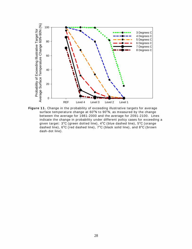
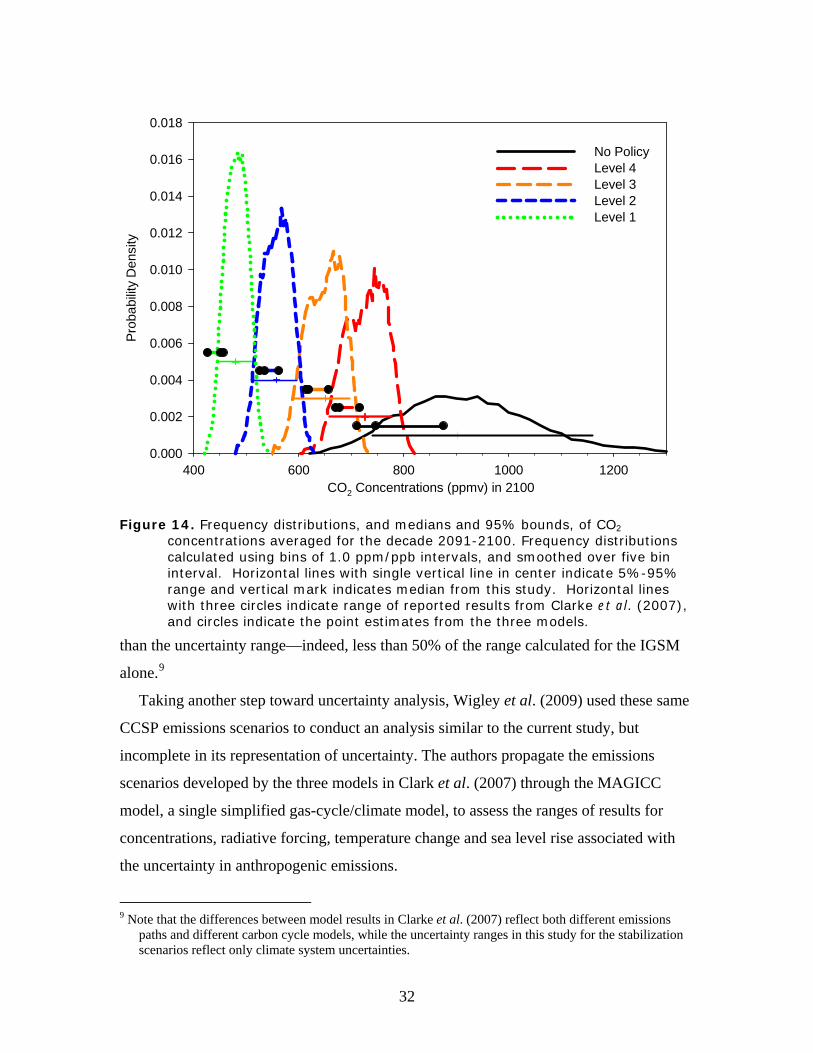
Figure 14 shows why this warning was warranted and illustrates the limitations of
multi-model assessments as a basis for forming judgments about uncertainty. For the
reference and each constraint, Level 1 through Level 4, the figure repeats the probability
distributions of CO2 concentrations in 2091-2100 from Figure 2a. Also shown in Figure
14 are five horizontal lines with black circles indicating the range of point estimates from
the different models in Clarke et al. (2007) for the particular policy scenario. For the
IGSM, the reference case used in the CCSP study is below the median in the current
calculations, in part because of model changes since the earlier analysis was done. But
what is important for this comparison is the magnitude in estimated uncertainty between
the two approaches. In all cases, the range of model point estimates is much narrower
31
CO2 Concentrations (ppmv) in 2100400 600 800 1000 1200
Prob
abilit
y D
ensi
ty
0.000
0.002
0.004
0.006
0.008
0.010
0.012
0.014
0.016
0.018
No PolicyLevel 4Level 3Level 2Level 1
Figure 14. Frequency distributions, and medians and 95% bounds, of CO2 concentrations averaged for the decade 2091-2100. Frequency distributions calculated using bins of 1.0 ppm/ppb intervals, and smoothed over five bin interval. Horizontal lines with single vertical line in center indicate 5%-95% range and vertical mark indicates median from this study. Horizontal lines with three circles indicate range of reported results from Clarke et al. (2007), and circles indicate the point estimates from the three models.
than the uncertainty range—indeed, less than 50% of the range calculated for the IGSM
alone.9
Taking another step toward uncertainty analysis, Wigley et al. (2009) used these same
CCSP emissions scenarios to conduct an analysis similar to the current study, but
incomplete in its representation of uncertainty. The authors propagate the emissions
scenarios developed by the three models in Clark et al. (2007) through the MAGICC
model, a single simplified gas-cycle/climate model, to assess the ranges of results for
concentrations, radiative forcing, temperature change and sea level rise associated with
the uncertainty in anthropogenic emissions.
9 Note that the differences between model results in Clarke et al. (2007) reflect both different emissions
paths and different carbon cycle models, while the uncertainty ranges in this study for the stabilization scenarios reflect only climate system uncertainties.
32
Climate related uncertainty in temperature change was estimated using just the
emissions scenario from the MiniCAM model, with uncertainty in system response
represented just by the lower and upper bounds from the IPCC’s 90% confidence interval
for climate sensitivity: 1.5oC and 6.0oC. It is then asserted that, because contributions
from uncertainties in other climate parameters are much smaller, the resulting ranges of
temperature change should represent the 90% confidence interval on temperature change
(conditional, of course, on a given emissions projection). The 90% ranges in this study
are 3.5oC to 7.4oC for No Policy and 0.7oC to 2.4oC for Level 1 cases, with median
warming of 2.8oC and 1.4oC, respectively.
The 90% range for the no-policy case in our study that can be compared with the
Wigley et al. (2009) estimate is the range for a single (median) emissions projection as
estimated by Sokolov et al. (2009b) which is 3.8oC to 7.0oC, whereas our range for Level
1 is 1.2oC to 2.4oC.10
Our median warming is larger in both cases, with values of 5.1oC and 1.8oC,
respectively. In the no-policy case, the difference is partly due to higher emissions; for
example, Wigley et al. (2009) calculate a 3.5oC warming for EPPA no-policy emissions.
Because the median value of climate sensitivity in our simulations (2.9 oC) is very close
to the median value used by Wigley et al. (2009), the remainder of the differences
between the two studies is the result of differences in the heat uptake by the ocean and
radiative forcing. While our absolute 90% range for temperature changes in the no-policy
case is slightly wider than the one in Wigley et al. (2009), our relative ranges are
narrower for both scenarios: from 26% below the median to 360% above the median for
no-policy and from -31% to 39% for Level 1. The smaller uncertainty ranges in our
projections of surface warming is explained by the fact that we use a joint probability
distribution of climate sensitivity, aerosol forcing, and ocean heat uptake that is
constrained by the climate change observed during 20th century. As discussed by Forest
et al. (2008), 20th century climate changes rule out low values of climate sensitivity (our
90% range is 2.0oC to 5.0oC) and also impose correlation between climate sensitivity, the
rate of ocean heat uptake, and the strength of aerosol forcing.
10 The comparison of results is not exact since Wigley et al. (2009) show the difference between values at
2100 and 2000 rather than between 2091-2100 and 1981-2000 averages.
33

0 2 4 6 8 10 12
Cum
ulat
ive
Prob
abilit
y
0.0
0.2
0.4
0.6
0.8
1.0
No PolicyLevel 4Level 3Level 2Level 1
Figure 15. Cumulative probability distributions of global mean temperature change from decadal average for 1861-1870 (preindustrial) to the decadal average for 2091-2100.
As a consequence of the above differences, the likelihood of meeting a temperature
target of 2oC above preindustrial (adding 0.7oC to the calculated results to include the
warming since pre-industrial) under the Level 1 policy differs between these two studies.
Wigley et al. (2009) estimate a 50% probability whereas the relatively small change in
the lower tail of the distribution in our analysis lowers this probability to only 20%
(Figure 15).
Another example of partial uncertainty analysis is the IPCC Fourth Assessment Report
(AR4), which presented probability bounds on some of its projections, conditional on
each of several different SRES emission scenarios (Nakicenovic et al., 2000). These
scenarios together with the 90% range of results from the IPCC AR4 AOGCMs (where
available), and the distribution of temperature change from our simulations, are shown in
Figure 16. This comparison suggests that the IPCC projections significantly
underestimate the risks of climate change in the absence of an emissions constraint. The
significantly larger chance of greater climate change in this study than in the IPCC is due
to both the emissions scenarios and the climate response. Detailed comparisons of
34
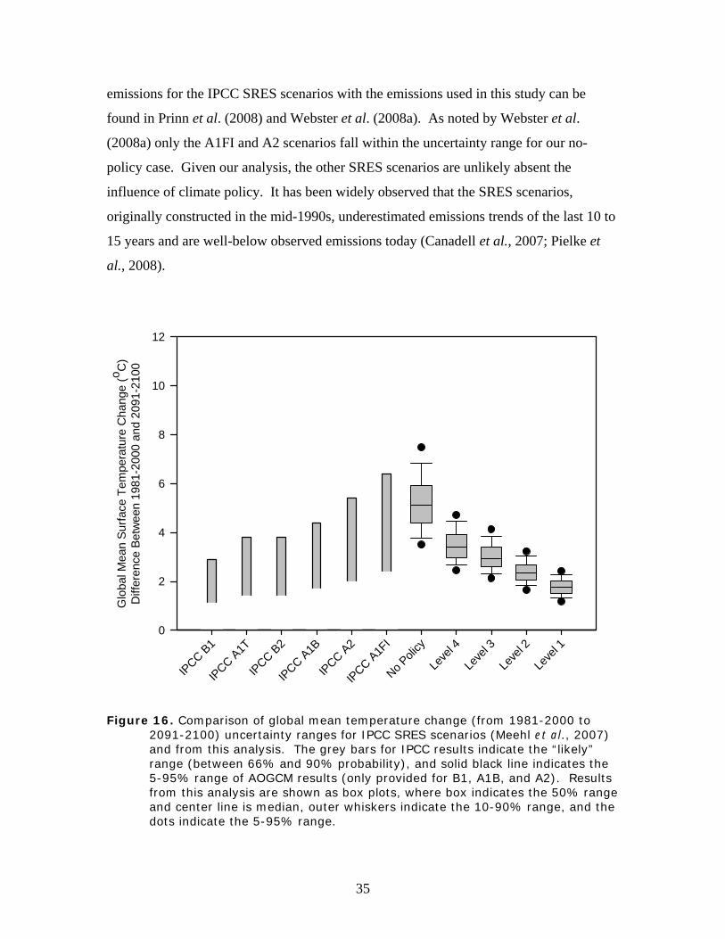
emissions for the IPCC SRES scenarios with the emissions used in this study can be
found in Prinn et al. (2008) and Webster et al. (2008a). As noted by Webster et al.
(2008a) only the A1FI and A2 scenarios fall within the uncertainty range for our no-
policy case. Given our analysis, the other SRES scenarios are unlikely absent the
influence of climate policy. It has been widely observed that the SRES scenarios,
originally constructed in the mid-1990s, underestimated emissions trends of the last 10 to
15 years and are well-below observed emissions today (Canadell et al., 2007; Pielke et
al., 2008).
IPCC B1
IPCC A1T
IPCC B2
IPCC A1B
IPCC A2
IPCC A1FI
No Poli
cy
Leve
l 4
Leve
l 3
Leve
l 2
Leve
l 1
Glo
bal M
ean
Surfa
ce T
empe
ratu
re C
hang
e (o C
)D
iffer
ence
Bet
wee
n 19
81-2
000
and
2091
-210
0
0
2
4
6
8
10
12
Figure 16. Comparison of global mean temperature change (from 1981-2000 to 2091-2100) uncertainty ranges for IPCC SRES scenarios (Meehl et al., 2007) and from this analysis. The grey bars for IPCC results indicate the “likely” range (between 66% and 90% probability), and solid black line indicates the 5-95% range of AOGCM results (only provided for B1, A1B, and A2). Results from this analysis are shown as box plots, where box indicates the 50% range and center line is median, outer whiskers indicate the 10-90% range, and the dots indicate the 5-95% range.
35
With regard to the climate response, Prinn et al. (2008) compared the IGSM forced by
the anthropogenic emissions for SRES scenarios and showed significantly higher surface
warming than that produced by the IPCC AR4 AOGCMs. The difference is explained by
a few factors. Due to a different treatment of carbon-nitrogen interactions, the terrestrial
carbon uptake simulated by the IGSM is smaller than the one simulated by the carbon-
cycle model used by the IPCC. The IGSM also takes into account climate change related
increases in the natural emissions of methane and N2O. As a result, greenhouse gas
concentrations simulated by the IGSM for a given SRES scenario are higher than the
concentrations for the same scenario used to force the AOGCMs in the simulations
described in IPCC AR4 (Meehl et al, 2007). As can be seen from results presented by
Prinn et al. (2008), changes in surface air temperature (SAT) in the IGSM simulations
with median no-policy, Level 4 and Level 2 emissions are very close to surface warming
obtained in simulations in which the IGSM was forced by the IPCC concentrations for
A1FI, A1B and B1 scenarios, respectively. In addition, the rates of oceanic heat uptake
for almost all of the AR4 AOGCMs lie in the upper half of the range implied from the
Levitus et al. (2005) estimates of the 20th century changes in the heat content of the deep
ocean. As shown by Sokolov et al. (2009a), surface warming projections obtained in the
IGSM simulations with climate input parameter distributions based on the Domingues et
al. (2008) estimates of changes in deep ocean heat content are closer to the results of the
IPCC AR4 AOGCMs.
As can be seen from Figure 16, the “likely”11, ranges given by the IPCC AR4 are
significantly wider than both 90% ranges in the simulations with the MIT IGSM and the
90% probability ranges based on the simulations with the AR4 AOGCMs. Meehl et al.
(2007) construct a “likely” range for temperature change of 40% below the best estimate
to 60% above the best estimate, with the best estimate being a mean value of surface
warming projected by the AOGCMs. The long upper tail of the “likely” range is
explained, in part, by the possibility of a strong positive feedback between climate and
the carbon cycle (Knutti et al., 2008). As mentioned above, taking into account the
nitrogen limitation on terrestrial carbon uptake makes this feedback much weaker
(Sokolov et al., 2008). However, as noted earlier, ocean data and other aspects of the
11 IPCC defines “likely” as having a probability of greater than 66% but less than 90%.
36
analysis, if varied produce a different range, and so a meta-analysis across these different
data sources and approaches would yield still greater uncertainty. A detailed comparison
between our no-policy case and the IPCC AR4 results is given by Sokolov et al. (2009).
Currently, a new round of scenario analyses is underway that would provide for a
common basis for climate model runs in the IPCC AR5. Guidance for those scenarios is
provided in Moss et al. (2008). Four Representative Concentration Pathways (RCPs) are
being prepared, which are described as: “one high pathway for which radiative forcing
reaches > 8.5 W/m2 by 2100 and continues to rise for some amount of time; two
intermediate "stabilization pathways" in which radiative forcing is stabilized at
approximately 6 W/m2 and 4.5 W/m2 after 2100; and one pathway where radiative
forcing peaks at approximately 3 W/m2 before 2100 and then declines.” The radiative
forcing increase in the RCPs is specified from the preindustrial level. All RCP pathways
reflect cases in the published literature with the first three based on the CCSP scenarios.
Thus, not coincidentally, the analysis reported here is approximately consistent with the
RCP scenarios. In particular, the median of our no-policy case (see Table 1) — when
corrected to a change from pre-industrial by the addition of an estimated of 1.8 W/m2
increase12 — is consistent with the “high and rising” RCP, while our Level 2 (3.5 + 1.8 =
5.3 W/m2 above preindustrial by 2100) and Level 1 (2.4 + 1.8 = 4.2 W/m2) are roughly
consistent with achieving stabilization sometime after 2100 at 6.0 and 4.5 W/m2
respectively.13 The analysis presented here thus may provide an assessment of
uncertainty to complement the scenario analysis being developed for the IPCC AR-5.
5. DISCUSSION Deciding a response to the climate threat is a challenge of risk management, where
choices about emissions mitigation must be made in the face of a cascade of
uncertainties: the emissions if no action is taken (and thus the cost of any level of
control), the response of the climate system to various levels of control, and the social
12 Our estimate of 1.8 W/m2 is derived from the GISS model (Hansen et al., 1988), the radiation code from
which is used in the MIT IGSM. The IPCC estimates the change in radiative forcing from preindustrial to present to be 1.6 W/m2, based on their estimates of the forcing from individual GHGs (Forster et al., 2007).
13 We do not have a case comparable to the 3 W/m2 as that was not in the CCSP scenario design, and presents considerable challenges in simulating as it requires technologies with net negative emissions.
37
and environmental consequences of the change that may come. In policy deliberations,
analysis of the very complex issues of climate change effects frequently is put aside, to be
replaced with a global target intended to avoid “danger”—stated, depending on the
context, in terms of a maximum allowable global temperature change, a maximum
allowable increase in radiative forcing, or a maximum total of anthropogenic emissions
of greenhouse gases over some long run period, usually a century. And, usually, the
relationship between these different measures is expressed without representing the
uncertainty among them, stating uncontrolled emissions in the form of a set of scenarios
and representing climate processes in the form of single “reference” or sometime median
values. For example, a widely-held position in climate discussions is that limiting
atmospheric concentrations of CO2 to 450 ppm (or 550 ppm CO2-eq) will achieve the
target of a maximum of 2oC temperature increase from the pre-industrial level. Major
issues of international negotiation, and potential economic cost, attend these
relationships, and it should be helpful to international discussions to have an analysis of
the likelihood that this relationship holds true, Here we have provided such an analysis,
and as shown in Section 4, the impression of the effectiveness of commonly-discussed
emissions limits can look very different when this human-climate system is subjected to a
more complete uncertainty analysis than normally is available.
Several qualifications about these results are worth mentioning. The resulting
uncertainties presented are conditional on the structural formulations of the MIT IGSM.
Distributions from other models, while likely different, would be similarly conditional.
Also, there are sources of uncertainty that are not treated here because of our current
inability to represent the relevant processes in a systematic and efficient fashion.
Additionally, the climate uncertainties presented here result from known or expected
sources of parametric uncertainty, and do not account for unanticipated changes or
shocks to the system that may occur. Also, as noted above, our projections of the climate
response to human forcing are conditional on the estimated joint distribution of input
parameters based on 20th century data series, importantly including a series for changes in
the heat content of the deep ocean. As indicated by Sokolov et al. (2009b) the use of an
alternative study of available ocean data (Domingues et al., 2008) leads to a decrease in
the simulated surface warming at the end of 21st century. Median surface warming in the
38

no-policy case decreases from 5.1oC to 4.1oC. Based on the results of Sokolov et al.
(2009a), a similar decrease should be expected in the transient surface air temperature
changes over the 21st century in simulations with climate policies.14
Of course, analyses focused on long-term emissions targets give only a partial picture
of the decision problem that nations face. A more complete framing would consider the
possibility of learning and revision of targets over time (e.g., Webster et al., 2008; Yohe
et al., 2004; Kolstad et al., 1996). Emissions goals agreed in the next decade or two can
and likely will be revised as new information comes to light. Nevertheless, the
representation of the problem given here can refocus the debate away from the illusion of
deterministic choices towards a risk management perspective.
14 It is worth mentioning that while estimate for changes in ocean heat content provided by Domingues et
al. (2008) suggests larger rate of the oceanic heat uptake, it also suggest higher values of climate sensitivity and, therefore, larger final equilibrium warming for the same concentrations of GHGs.
39

6. REFERENCES
Bonan, G.B., K.W. Oleson, M. Vertenstein, S. Lewis, X. Zeng, Y. Dai, R.E. Dickinson, and Z.-L. Yang, 2002: The Land Surface Climatology of the Community Land Model Coupled to the NCAR Community Climate Model. J. Climate, 15: 3123-3149.
Calbó, J., W. Pan, M. Webster, R.G. Prinn, and G.J. McRae, 1998: Parameterization of Urban Sub-Grid Scale Processes in Global Atmospheric Chemistry Models. J. Geophysical Research, 103: 3437-3451.
Canadell, J.G., C. Le Quéré, M.R. Raupach, C.B. Field, E.T. Buitenhuis, P. Ciais, T.J. Conway, N.P. Gillett, R.A. Houghton, and G. Marland, 2007: Contributions to Accelerating Atmospheric CO2 Growth from Economic Activity, Carbon Intensity, and Efficiency of Natural Sinks. Proceeding of the National Academy of Sciences, 104:18866-18870; published online before print October 25, 2007, doi:10.1073/pnas.0702737104.
Clarke, L., J. Edmonds, H. Jacoby, H. Pitcher, J. Reilly, and R. Richels, 2007: Scenarios of Greenhouse Gas Emissions and Atmospheric Concentrations, Sub-report 2.1A of Synthesis and Assessment Product 2.1 by the U.S. Climate Change Science Program and the Subcommittee on Global Change Research,, Department of Energy, Office of Biological and Environmental Research, Washington, DC., USA, 106pp.
Domingues, C.M., J.A. Church, N.J. White, P.J. Gleckler, S.E. Wijffels, P.M. Barker, and J.R. Dunn, 2008: Improved Estimates of Upper-Ocean Warming and Multi-Decadal Sea-Level Rise. Nature, 453: 1090-1094.
Felzer, B., D. Kicklighter, J. Melillo, C. Wang, Q. Zhuang, and R. Prinn, 2004: Effects of Ozone on Net Primary Production and Carbon Sequestration in the Conterminous United States Using a Biogeochemistry Model. Tellus, 56B: 230-248.
Fisher, B.S., N. Nakicenovic, K. Alfsen, J. Corfee Morlot, F. de la Chesnaye, J.-Ch. Hourcade, K. Jiang, M. Kainuma, E. La Rovere, A. Matysek, A. Rana, K. Riahi, R. Richels, S. Rose, D. van Vuuren, R. Warren, 2007: Issues Related to Mitigation in the Long Term Context. In: Climate Change 2007: Mitigation. Contribution of Working Group III to the Fourth Assessment Report of the Inter-governmental Panel on Climate Change, B. Metz, O.R. Davidson, P.R. Bosch, R. Dave, L.A. Meyer (eds.), Cambridge University Press, Cambridge, U.K.
Forest, C.E., P.H. Stone and A.P. Sokolov, 2008: Constraining Climate Model Parameters from Observed 20th Century Changes. Tellus, 60A: 911-920.
Forster, P., V. Ramaswamy, P. Artaxo, T. Berntsen, R. Betts, D.W. Fahey, J. Haywood, J. Lean, D.C. Lowe, G. Myhre, J. Nganga, R. Prinn, G. Raga, M. Schulz and R. Van Dorland, 2007: Changes in Atmospheric Constituents and in Radiative Forcing. In: Climate Change 2007: The Physical Science Basis. Contribution of Working Group I to the Fourth Assessment Report of the Intergovernmental Panel on Climate Change, Solomon, S., D. Qin, M. Manning, Z. Chen, M. Marquis, K.B. Averyt, M.Tignor and H.L. Miller (eds.), Cambridge University Press, Cambridge, U.K.
G8 Summit, 2009. Chair’s Summary, 10 July 2009. (www.guitalia2009.it/static/G8_Allegato/Chair_Summary,1.pdf).
Hansen, J., I. Fung, A. Lacis, D. Rind, S. Lebedeff, R. Ruedy and G. Russel, 1988: Global Climate Change As Forecast By Goddard Institute For Space Studies Three-
40
Dimensional Model, J Geoph Res 93: 9341-9364. Huang, J., R. Wang, R. Prinn and D. Cunnold, 2009: A Semi-Empirical Representation of
the Temporal Variation of Total Greenhouse Gas Levels Expressed as Equivalent Levels of Carbon Dioxide. MIT JPSPGC, Report 174, 10pp. (http://globalchange.mit.edu/files/document/MITJPSPGC_Rpt174.pdf).
Iman, R.L., and W.J. Conover, 1982: A Distribution-Free Approach to Inducing Rank Correlation among Input Variables. Communications in Statistics, B11(3): 311-334.
Ishii, M., and M. Kimoto, 2009: Reevaluation of Historical Ocean Heat Content Variations with Time-Varying XBT and MBT Depth Bias Corrections. Journal of Oceanography, 65: 287-299.
Knutti, R., M.R. Allen, P. Friedlingstein, J.M. Gregory, G.C. Hegerl, G.A. Meehl, M. Meinshausen, J.M. Murphy, G.-K. Plattner, S.C.B. Raper, T.F. Stocker, P.A. Stott, H. Teng, and T.M.L Wigley. 2008: A Review of Uncertainties in Global Temperature Projections over the Twenty-First Century. J. Climate, 21: 2651–2663.
Kolstad, C.D., 1996: Learning and Stock Effects in Environmental Regulation: The Case of Greenhouse Gas Emissions. Journal of Environmental Economics and Management, 31: 1-18.
Levitus, S., J.I. Antonov, T.P. Boyer, R.A. Locarnini, H.E. Garcia, and A.V. Mishonov, 2009: Global Ocean Heat Content 1955–2008 in Light of Recently Revealed Instrumentation Problems. Geophysical Research Letters, 36(L07608), doi:10.1029/2008GL037155.
Levitus, S., J. Antonov, and T.P. Boyer, 2005: Warming of the World Ocean, 1955–2003. Geophys. Res. Lett., 32(L02604), http://dx.doi.org/doi:10.1029/2004GL021592.
Liu, Y., 1996: Modeling the Emissions of Nitrous Oxide (N2O) and Methane (CH4) from the Terrestrial Biosphere to the Atmosphere. Ph.D. Thesis. MIT JPSPGC, Report 10, 219 pp. (Available on line at http://web.mit.edu/globalchange/www/MITJPSPGC_Rpt10.pdf).
Mayer, M., C. Wang, M. Webster, and R.G. Prinn, 2000: Linking Local Air Pollution to Global Chemistry and Climate, J. Geophysical Research, 105(D18): 22,869-22,896.
McKay, M.D., W.J. Conover, et al., 1979: A Comparison of Three Methods for Selecting Values of Input Variables in the Analysis of Output from a Computer Code. Technometrics, 21(2): 239-245.
Meehl, G.A., T.F. Stocker, W.D. Collins, P. Friedlingstein, A.T. Gaye, J.M. Gregory, A. Kitoh, R. Knutti, J.M. Murphy, A. Noda, S.C.B. Raper, I.G. Watterson, A.J. Weaver and Z.-C. Zhao, 2007: Global Climate Projections. In: Climate Change 2007: The Physical Science Basis. Contribution of Working Group I to the Fourth Assessment Report of the Intergovernmental Panel on Climate Change, S. Solomon, D. Qin, M. Manning, Z. Chen, M. Marquis, K.B. Averyt, M. Tignor, and H.L. Miller (eds.). Cambridge University Press, Cambridge, United Kingdom and New York, NY, USA.
Moss, R., M. Babiker, S. Brinkman, E. Calvo, T. Carter, J. Edmonds, I. Elgizouli, S. Emori, L. Erda, K. Hibbard, R. Jones, M. Kainuma, J.Kelleher, J. Francois Lamarque, M. Manning, B. Matthews, J. Meehl, L. Meyer, J. Mitchell, N. Nakicenovic, B. O’Neill, R. Pichs, K. Riahi, S. Rose, P. Runci, R. Stouffer, D. van Vuuren, J. Weyant, T. Wilbanks, J. Pascal van Ypersele, M. Zurek, F. Birol, P. Bosch, O. Boucher, J. Feddema, A. Garg, A. Gaye, M. Ibarraran, E. La Rovere, B. Metz, S. Nishioka, H.
41
Pitcher, D. Shindell, P.R. Shukla, A. Snidvongs, P. Thorton, V. Vilariño, 2007. Towards New Scenarios for Analysis of Emissions, Climate Change, Impacts, and Response Strategies, IPCC Expert Meeting Report, 19–21 September, 2007 Noordwijkerhout, The Netherlands, http://ipcc-data.org/docs/ar5scenarios/IPCC_Final_Draft_Meeting_Report_3May08.pdf.
Nakicenovic, N., et al., 2000: Special Report on Emissions Scenarios, Intergovernmental Panel on Climate Change. Cambridge University Press, Cambridge, UK.
Pielke, R., T. Wigley, C. Green, 2008: Dangerous Assumptions. Nature, 452: 531-532, 2 April 2008. doi:10.1038/452531a.
Paltsev, S., J.M. Reilly, H.D. Jacoby, R.S. Eckaus, J. McFarland, M. Sarofim, M. Asadoorian, and M. Babiker, 2005: The MIT Emissions Prediction and Policy Analysis (EPPA) Model: Version 4, MIT JPSPGC, Report 125, Cambridge, MA. See http://globalchange.mit.edu/pubs/abstract.php?publication_id=697.
Prinn, R., J. Reilly, M. Sarofim, C. Wang, and B. Felzer, 2007: Effects of Air Pollution Control on Climate: Results from an Integrated Assessment Model. In: Human-induced Climate Change: An Interdisciplinary Assessment, M.E. Schlesinger, H.S. Kheshgi, J. Smith, F.C. de la Chesnaye, J.M. Reilly, T. Wilson, and C. Kolstad (eds.). Cambridge University Press, Cambridge, UK.
Prinn, R., S. Paltsev, A. Sokolov, M. Sarofim, J. Reilly, and H. Jacoby, 2008: The Influence on Climate Change of Differing Scenarios for Future Development Analyzed Using MIT Integrated Global System Model. MIT JPSPGC, Report 163, Cambridge, MA. Available at: http://globalchange.mit.edu/files/document/MITJPSPGC_Rpt163.pdf.
Ramaswamy, V., O. Boucher, J. Haigh, D. Hauglustaine, J. Haywood, G. Myhre, T. Nakajima, G.Y. Shi, S. Solomon, R. Betts, R. Charlson, C. Chuang, J.S. Daniel, A. Del Genio, R. van Dorland, J. Feichter, J. Fuglestvedt, P.M. de F. Forster, S.J. Ghan, A. Jones, J.T. Kiehl, D. Koch, C. Land, J. Lean, U. Lohmann, K. Minschwaner, J.E. Penner, D.L. Roberts, H. Rodhe, G.J. Roelofs, L.D. Rotstayn, T.L. Schneider, U. Schumann, S.E. Schwartz, M.D. Schwarzkopf, K.P. Shine, S. Smith, D.S. Stevenson, F. Stordal, I. Tegen, Y. Zhang, 2001: Radiative Forcing of Climate Change. In: Climate Change 2001: The Scientific Basis. Contribution of Working Group I to the Third Assessment Report of the Intergovernmental Panel on Climate Change. J.T. Houghton,Y. Ding, D.J. Griggs, M. Noguer, P.J. van der Linden, X. Dai, K. Maskell, and C.A. Johnson (eds.). Cambridge University Press, Cambridge, United Kingdom and New York, NY, USA, 881pp.
Rubinstein, R.Y., and D.P. Kroese, 2008: Simulation and the Monte Carlo Method. John Wiley & Sons, Hoboken, N.J.
Schlosser, C.A., D. Kicklighter and A. Sokolov, 2007: A Global Land System Framework for Integrated Climate-Change Assessments. MIT JPSPGC, Report 147. Massachusetts Institute of Technology, Cambridge, Massachusetts. (see also http://globalchange.mit.edu/files/document/MITJPSPGC_Rpt147.pdf).
Schneider, S.H., S. Semenov, A. Patwardhan, I. Burton, C.H.D. Magadza, M. Oppenheimer, A.B. Pittock, A. Rahman, J.B. Smith, A Suarez, and F. Yamni, 2007: Assessing Key Vulnerabilities and the Risk Form Climate Change. In: Climate
42

Change 2007: Impacts, Adaptation and Vulnerability. Contribution of Working Group II to the Fourth Assessment Report of the Intergovernmental Panel on Climate Change, M.L. Parry, O.F. Canziani, J.P. Palutikof, P.J. van der Linden, and C.E. Hanson, (eds.). Cambridge University Press, Cambridge, UK, 779-810.
Sokolov, A.P., C.E. Forest, and P.H. Stone, 2009: Sensitivity of Climate Change Projections to Uncertainties in the Estimates of Observed Changes in Deep-Ocean Heat Content. Climate Dynamics, 2009a. Available online: http://www.springerlink.com/content/u513846q4133k712/fulltext.pdf
Sokolov, A.P., P.H. Stone, C.E. Forest, R. Prinn, M.C. Sarofim, M. Webster, S. Paltsev, C.A. Schlosser, D. Kicklighter, S. Dutkiewicz, J. Reilly, C. Wang, B Felzer, H.D. Jacoby, 2009b: Probabilistic Forecast for 21st Century Climate Based on Uncertainties in Emissions (without policy) and Climate Parameters. Journal of Climate 22: 5175-5204.
Sokolov, A.P., D.W. Kicklighter, J.M. Melillo, B.S. Felzer, C.A. Schlosser, and T.W. Cronin, 2008: Consequences of Considering Carbon-Nitrogen Interactions on the Feedbacks between Climate and the Terrestrial Carbon Cycle. Journal of Climate, 21: 3776-3796, doi: 10.1175/2008JCLI2038.1.
Sokolov, A.P., S. Dutkiewicz, P.H. Stone, and J.R. Scott, 2007: Evaluating the Use of Ocean Models of Different Complexity in Climate Change Studies. MIT JPSPGC, Report 128, 23 pp. (Available on line at: http://web.mit.edu/globalchange/www/MITJPSPGC_Rpt128.pdf).
Sokolov, A.P., C.A. Schlosser, S. Dutkiewicz, S. Paltsev, D.W. Kicklighter, H.D. Jacoby, R.G. Prinn, C.E. Forest, J. Reilly, C. Wang, B. Felzer, M.C. Sarofim, J. Scott, P.H. Stone, J.M. Melillo, and J. Cohen, 2005: The MIT Integrated Global System Model (IGSM) Version 2: Model Description and Baseline Evaluation, MIT JPSPGC, Report 124, 40 pp. (Available on line at: http://web.mit.edu/globalchange/www/MITJPSPGC_Rpt124.pdf).
Sokolov A., C. Forest, and P.H. Stone, 2003: Comparing Oceanic Heat Uptake in AOGCM Transient Climate Change Experiments. J Climate, 16: 1573-1582.
Sokolov, A., and P. Stone, 1998: A Flexible Climate Model for Use in Integrated Assessments. Climate Dynamics, 14: 291-303.
Stern, D., 2006: Reversal of the Trend in Global Anthropogenic Sulfur Emissions. Global Environmental Change, 16(2): 207-220.
Stern, D., 2005: Beyond the Environmental Kuznets Curve: Diffusion of Sulfur-Emissions-Abating Technology. Journal of Environment & Development, 14(1): 101-124.
Tol, R.S.J., 2005: The Marginal Damage Costs of Carbon Dioxide Emissions: An Assessment of the Uncertainties. Energy Policy, 33(16): 2064–2074.
Ulph, A. and D. Ulph, 1997: Global Warming, Irreversibility and Learning. Economic Journal, 107(442): 636-650.
United Nations, 1992: Framework Convention on Climate Change. International Legal Materials, 31: 849-873.
UN FCCC [United Nations Framework Convention on Climate Change], 1997: Bali Action Plan (FCCC/CP/2007/6 Add.1).
43
44
Wang, C., R.G. Prinn, and A. Sokolov, 1998: A Global Interactive Chemistry and Climate Model: Formulation and Testing. J. Geophys. Res., 103: 3399-3418.
Webster, M.D., S. Paltsev, J. Parsons, J. Reilly, and H. Jacoby, 2008a: Uncertainty in Greenhouse Emissions and Costs of Atmospheric Stabilization, MIT JPSPGC, Report 165. (Available online at http://web.mit.edu/globalchange/www/MITJPSPGC_Rpt165.pdf )
Webster, M.D., L. Jakobovits, and J. Norton, 2008b: Learning about Climate Change and Implications for Near-term Policy. Climatic Change, 89(1-2): 67-85.
Webster, M.D., M. Babiker, M. Mayer, J.M. Reilly, J. Harnisch, M.C. Sarofim, and C. Wang, 2002: Uncertainty in Emissions Projections for Climate Models. Atmospheric Environment, 36(22): 3659-3670.
Webster, M., C. Forest, J. Reilly, M. Babiker, D. Kicklighter, M. Mayer, R. Prinn, M. Sarofim, A. Sokolov, P. Stone, and C. Wang, 2003: Uncertainty Analysis of Climate Change and Policy Response. Climatic Change, 62: 295-320.
Wigley, T. and S. Raper, 2001: Interpretation of High Projections for Global-Mean Warming. Science, 293, 20 July.
Wigley, T., L. Clarke, J. Edmonds, H. Jacoby, S. Paltsev, H. Pitcher, J. Reilly, R. Richels, M. Sarofim, and S. Smith, 2009: Uncertainties in Climate Stabilization. Climatic Change (in press).
Yohe, G., N. Andronova and M. Schlesinger, 2004: To Hedge or not against an Uncertain Climate Future? Science, 306: 416-417.
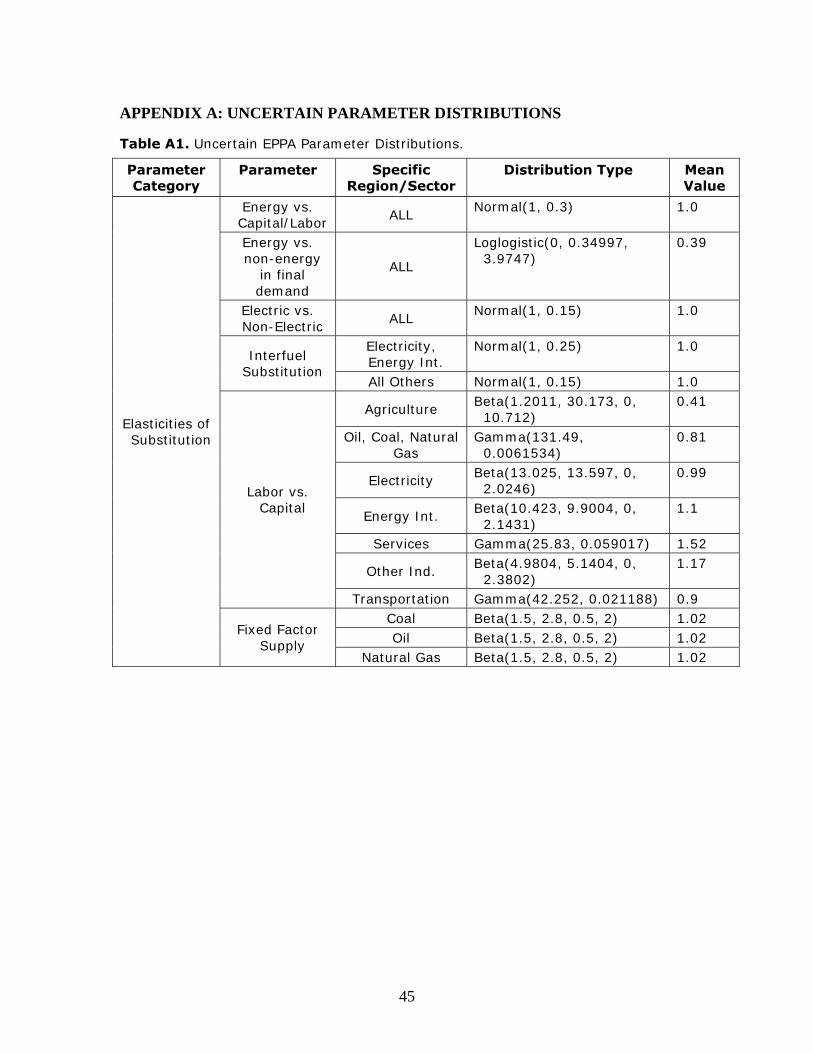
APPENDIX A: UNCERTAIN PARAMETER DISTRIBUTIONS
Table A1. Uncertain EPPA Parameter Distributions.
Parameter Category
Parameter Specific Region/Sector
Distribution Type Mean Value
Energy vs. Capital/Labor
ALL Normal(1, 0.3) 1.0
Energy vs. non-energy
in final demand
ALL
Loglogistic(0, 0.34997, 3.9747)
0.39
Electric vs. Non-Electric
ALL Normal(1, 0.15) 1.0
Electricity, Energy Int.
Normal(1, 0.25) 1.0 Interfuel
Substitution All Others Normal(1, 0.15) 1.0
Agriculture Beta(1.2011, 30.173, 0, 10.712)
0.41
Oil, Coal, Natural Gas
Gamma(131.49, 0.0061534)
0.81
Electricity Beta(13.025, 13.597, 0, 2.0246)
0.99
Energy Int. Beta(10.423, 9.9004, 0, 2.1431)
1.1
Services Gamma(25.83, 0.059017) 1.52
Other Ind. Beta(4.9804, 5.1404, 0, 2.3802)
1.17
Labor vs. Capital
Transportation Gamma(42.252, 0.021188) 0.9 Coal Beta(1.5, 2.8, 0.5, 2) 1.02 Oil Beta(1.5, 2.8, 0.5, 2) 1.02
Elasticities of Substitution
Fixed Factor Supply
Natural Gas Beta(1.5, 2.8, 0.5, 2) 1.02
45

Table A1 (continued). Uncertain EPPA Parameter Distributions.
Parameter Category
Parameter Specific Region/Sector
Distribution Type Mean Value
USA Pearson5(4.8295, 0.2) 0.06 CAN Pearson5(4.8295, 0.2) 0.06 MEX Beta(3.2252, 3.1, 0, 0.04) 0.02 JPN Beta(3.2, 4.7, 0.01, 0.16) 0.07 ANZ Beta(7.8, 7.8, 0, 0.08) 0.04 EUR Beta (2.8, 5.6, 0.03, 0.16) 0.07 EET Beta(5.6, 6.8, 0.02, 0.16) 0.08 FSU Beta(3.7, 5.6, 0, 0.16) 0.06 ASI Beta(2.1, 4.1, 0, 0.2) 0.07
CHN Loglogistic(0, 0.052, 3.4102)
0.06
IND Beta(7.6, 11.4, 0, 0.2) 0.08 IDZ Beta(3.2252, 3.1, 0, 0.04) 0.02 AFR Beta(3.2252, 3.1, 0, 0.04) 0.02
MES Beta(3.2294, 3.4608, 0, 0.04)
0.02
LAM Beta(3.2252, 3.1, 0, 0.04) 0.02
CH4 Elas. In Agriculture
ROW Beta(3.2294, 3.4608, 0, 0.065)
0.03
OECD Beta(8.7, 7.8, 0, 0.075) 0.04 LDC Beta(5.1, 5.3, 0, 0.037) 0.02 FSU Beta(7.8, 5.5, 0.01, 0.06) 0.04
Abatement Cost
Elasticities
N2O Elas. In Agriculture
EET Beta(4.2, 4.3, 0, 0.08) 0.04 Vintaging ALL Gamma(10.429, 0.049431) 0.52
SO2 Beta(7, 3, -0.1, -0.005) -0.03 NOx Beta(7, 3, -0.03, -0.005) -0.01 BC Beta(7, 3, -0.1, -0.005) -0.03 OC Beta(7, 3, -0.1, -0.005) -0.03 VOC Beta(7, 3, -0.03, -0.005) -0.01 CO Beta(7, 3, -0.03, -0.005) -0.01
Urban Emission Trends
NH3 Beta(7, 3, -0.03, -0.005) -0.01
46
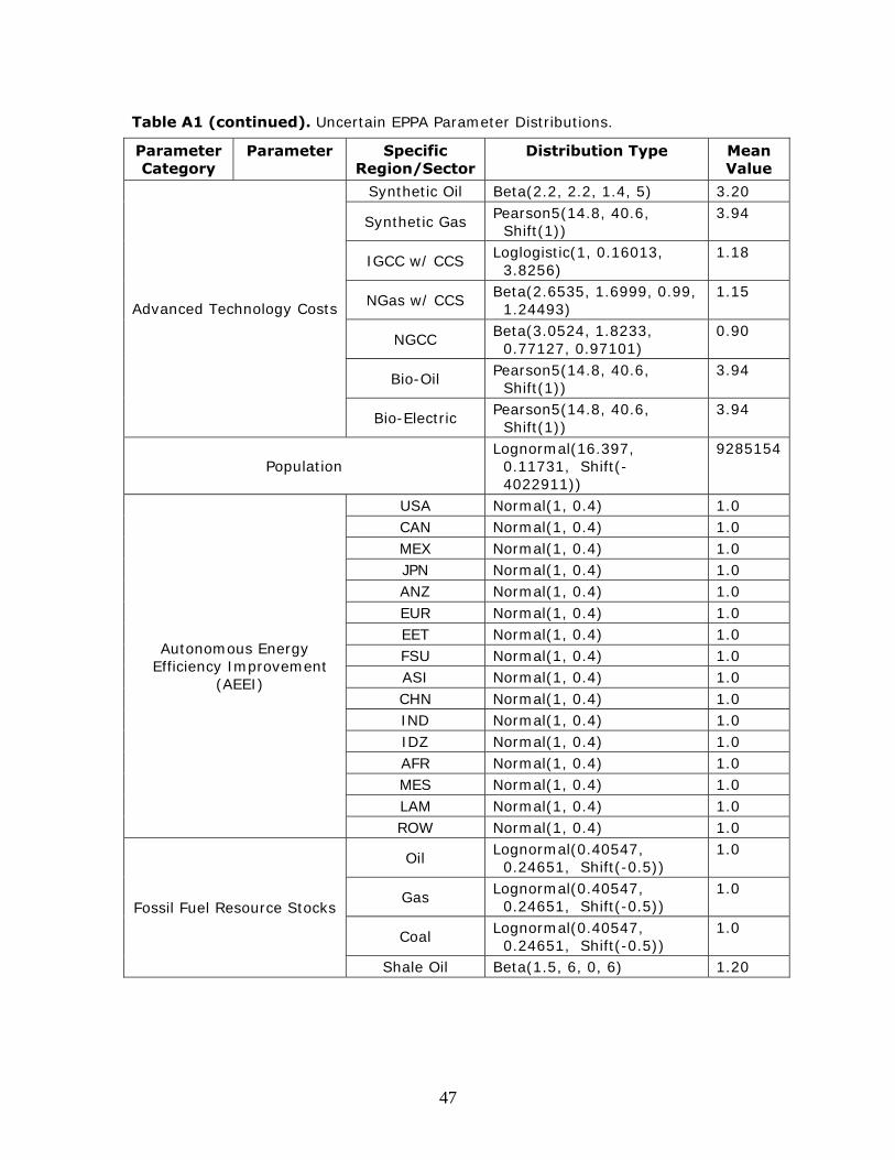
Table A1 (continued). Uncertain EPPA Parameter Distributions.
Parameter Category
Parameter Specific Region/Sector
Distribution Type Mean Value
Synthetic Oil Beta(2.2, 2.2, 1.4, 5) 3.20
Synthetic Gas Pearson5(14.8, 40.6, Shift(1))
3.94
IGCC w/ CCS Loglogistic(1, 0.16013, 3.8256)
1.18
NGas w/ CCS Beta(2.6535, 1.6999, 0.99, 1.24493)
1.15
NGCC Beta(3.0524, 1.8233, 0.77127, 0.97101)
0.90
Bio-Oil Pearson5(14.8, 40.6, Shift(1))
3.94
Advanced Technology Costs
Bio-Electric Pearson5(14.8, 40.6, Shift(1))
3.94
Population Lognormal(16.397,
0.11731, Shift(-4022911))
9285154
USA Normal(1, 0.4) 1.0 CAN Normal(1, 0.4) 1.0 MEX Normal(1, 0.4) 1.0 JPN Normal(1, 0.4) 1.0 ANZ Normal(1, 0.4) 1.0 EUR Normal(1, 0.4) 1.0 EET Normal(1, 0.4) 1.0 FSU Normal(1, 0.4) 1.0 ASI Normal(1, 0.4) 1.0 CHN Normal(1, 0.4) 1.0 IND Normal(1, 0.4) 1.0 IDZ Normal(1, 0.4) 1.0 AFR Normal(1, 0.4) 1.0 MES Normal(1, 0.4) 1.0 LAM Normal(1, 0.4) 1.0
Autonomous Energy Efficiency Improvement
(AEEI)
ROW Normal(1, 0.4) 1.0
Oil Lognormal(0.40547, 0.24651, Shift(-0.5))
1.0
Gas Lognormal(0.40547, 0.24651, Shift(-0.5))
1.0
Coal Lognormal(0.40547, 0.24651, Shift(-0.5))
1.0 Fossil Fuel Resource Stocks
Shale Oil Beta(1.5, 6, 0, 6) 1.20
47

Table A1 (continued). Uncertain EPPA Parameter Distributions.
Parameter Category
Parameter Specific Region/Sector
Distribution Type Mean Value
Nuclear Beta(1.2, 4, 0, 1.5) 0.35 CCS
Technologies Beta(1.5, 2.5, 0.3, 5.5) 2.25 Technology Penetration
Rates Wind/Solar Beta(1.1, 5, 0, 2) 0.36
USA Normal(1,0.3) 1.0 CAN Normal(1,0.3) 1.0 MEX Normal(1,0.3) 1.0 JPN Normal(1,0.3) 1.0 ANZ Normal(1,0.3) 1.0 EUR Normal(1,0.3) 1.0 EET Normal(1,0.3) 1.0 FSU Normal(1,0.3) 1.0 ASI Normal(1,0.3) 1.0 CHN Normal(1,0.3) 1.0 IND Normal(1,0.3) 1.0 IDZ Normal(1,0.3) 1.0 AFR Normal(1,0.3) 1.0 MES Normal(1,0.3) 1.0 LAM Normal(1,0.3) 1.0
SO2
ROW Normal(1,0.3) 1.0 CO Normal(1, 0.25) 1.0 BC Lognormal(-0.0812, 0.305) 1.0 OC Lognormal(-0.0812, 0.305) 1.0 NOx Lognormal(-0.0812, 0.305) 1.0 NH3 Lognormal(-0.0812, 0.305) 1.0
Urban Pollutant
Initial Inventories
VOC Lognormal(-0.0812, 0.305) 1.0 AGRI Beta(1.8, 1.8, 0.4, 1.6) 1.0 COAL Beta(2, 2, 0.89, 1.11) 1.0 GAS Beta(2, 2, 0.86, 1.14) 1.0 OIL Beta(2, 2, 0.86, 1.14) 1.0 EINT Beta(2, 2, 0.86, 1.14) 1.0
LANDFILL Beta(1.8, 1.8, 0.96, 1.04) 1.0
CH4 Emissions Factors
DSEWAGE Beta(1.8, 1.8, 0.96, 1.04) 1.0
48

APPENDIX B: RESULTS OF MONTE CARLO ANALYSIS OF IGSM
Table B1. Mean, standard deviation, and selected fractiles for increase in global mean temperature from the average for 1981-2000 to 2091-2100.
REF Level 4 Level 3 Level 2 Level 1
Mean 5.3 3.5 3.0 2.4 1.8 Stdev 1.2 0.7 0.6 0.5 0.4
2.5% 3.3 2.3 2.0 1.6 1.1
5.0% 3.5 2.5 2.1 1.7 1.2
25.0% 4.4 3.0 2.6 2.1 1.5
50.0% 5.1 3.4 2.9 2.3 1.8
75.0% 5.9 3.9 3.4 2.7 2.0
95.0% 7.4 4.7 4.1 3.2 2.4
Fractiles (Degrees
C)
97.5% 8.2 5.0 4.3 3.4 2.5
2.5% 0.6 0.7 0.7 0.7 0.6
5.0% 0.7 0.7 0.7 0.7 0.7
25.0% 0.9 0.9 0.9 0.9 0.9
50.0% 1.0 1.0 1.0 1.0 1.0
75.0% 1.2 1.2 1.2 1.1 1.2
95.0% 1.4 1.4 1.4 1.4 1.4
Fractiles (Relative
to Median)
97.5% 1.6 1.5 1.5 1.4 1.5
49
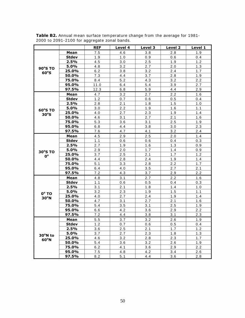
Table B2. Annual mean surface temperature change from the average for 1981-2000 to 2091-2100 for aggregate zonal bands.
REF Level 4 Level 3 Level 2 Level 1 Mean 7.5 4.6 3.8 2.8 1.9 Stdev 1.9 1.0 0.9 0.6 0.4 2.5% 4.5 3.0 2.5 1.9 1.2 5.0% 4.8 3.2 2.7 2.0 1.3
25.0% 6.2 3.8 3.2 2.4 1.7 50.0% 7.3 4.4 3.7 2.8 1.9 75.0% 8.4 5.2 4.3 3.2 2.2 95.0% 11.0 6.4 5.4 3.9 2.7
90oS TO 60oS
97.5% 12.3 6.8 5.9 4.4 2.9 Mean 4.7 3.2 2.7 2.2 1.6 Stdev 1.2 0.7 0.6 0.5 0.4 2.5% 2.8 2.1 1.8 1.5 1.0 5.0% 3.0 2.2 1.9 1.6 1.1
25.0% 4.0 2.7 2.3 1.9 1.4 50.0% 4.6 3.1 2.7 2.1 1.6 75.0% 5.3 3.6 3.1 2.5 1.9 95.0% 6.8 4.4 3.8 3.0 2.3
60oS TO 30oS
97.5% 7.6 4.7 4.1 3.2 2.4 Mean 4.5 2.9 2.5 2.0 1.4 Stdev 1.1 0.6 0.6 0.4 0.3 2.5% 2.7 1.9 1.6 1.3 0.9 5.0% 2.9 2.0 1.7 1.4 0.9
25.0% 3.7 2.5 2.1 1.7 1.2 50.0% 4.4 2.8 2.4 1.9 1.4 75.0% 5.1 3.3 2.8 2.2 1.7 95.0% 6.4 4.0 3.5 2.7 2.1
30oS TO 0o
97.5% 7.2 4.3 3.7 2.9 2.2 Mean 4.8 3.1 2.7 2.2 1.6 Stdev 1.1 0.6 0.5 0.4 0.3 2.5% 3.1 2.1 1.8 1.4 1.0 5.0% 3.2 2.3 1.9 1.5 1.1
25.0% 4.0 2.7 2.4 1.9 1.4 50.0% 4.7 3.1 2.7 2.1 1.6 75.0% 5.4 3.5 3.1 2.5 1.9 95.0% 6.6 4.2 3.6 2.9 2.2
0o TO 30oN
97.5% 7.2 4.4 3.8 3.1 2.3 Mean 5.5 3.7 3.2 2.6 1.9 Stdev 1.2 0.7 0.6 0.5 0.4 2.5% 3.6 2.5 2.1 1.7 1.2 5.0% 3.7 2.7 2.3 1.8 1.3
25.0% 4.6 3.2 2.8 2.3 1.7 50.0% 5.4 3.6 3.2 2.6 1.9 75.0% 6.2 4.1 3.6 2.9 2.2 95.0% 7.5 4.8 4.2 3.4 2.6
30oN to 60oN
97.5% 8.2 5.1 4.4 3.6 2.8
50
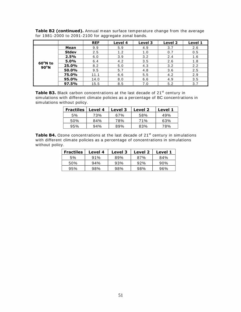
Table B2 (continued). Annual mean surface temperature change from the average for 1981-2000 to 2091-2100 for aggregate zonal bands.
REF Level 4 Level 3 Level 2 Level 1 Mean 9.9 5.9 4.9 3.7 2.6 Stdev 2.5 1.2 1.0 0.7 0.5 2.5% 6.0 3.9 3.2 2.4 1.6 5.0% 6.4 4.2 3.5 2.6 1.8
25.0% 8.2 5.0 4.3 3.2 2.2 50.0% 9.5 5.7 4.8 3.6 2.5 75.0% 11.1 6.6 5.5 4.2 2.9 95.0% 14.0 8.0 6.6 4.9 3.5
60oN to 90oN
97.5% 15.5 8.5 7.0 5.2 3.7
Table B3. Black carbon concentrations at the last decade of 21st century in simulations with different climate policies as a percentage of BC concentrations in simulations without policy.
Fractiles Level 4 Level 3 Level 2 Level 1 5% 73% 67% 58% 49% 50% 84% 78% 71% 63% 95% 94% 89% 83% 78%
Table B4. Ozone concentrations at the last decade of 21st century in simulations with different climate policies as a percentage of concentrations in simulations without policy.
Fractiles Level 4 Level 3 Level 2 Level 1 5% 91% 89% 87% 84% 50% 94% 93% 92% 90% 95% 98% 98% 98% 96%
51

APPENDIX C: PROBABILITIES OF EXCEEDING TARGETS
Table C1. Odds of Exceeding Illustrative Targets in Global Mean Surface Air Temperature Change from 1981-2000 average to 2091-2100 average in no-policy and Four Control Ensembles.
ΔT > 2oC ΔT > 4oC ΔT > 6oC No-Policy 400 in 400 17 in 20 1 in 4 Level 4 400 in 400 1 in 4 1 in 400 Level 3 97 in 100 7 in 100 <1 in 400 Level 2 8 in 10 1 in 400 <1 in 400 Level 1 1 in 4 <1 in 400 <1 in 400
Table C2. Probability of Exceeding Selected Targets in Average Surface Air Temperature Change over 60oN to 90oN from 1981-2000 average to 2091-2100 average.
ΔT > 4oC ΔT > 6oC ΔT > 8oC No-Policy 400 in 400 95 in 100 7 in 10 Level 4 95 in 100 3 in 10 3 in 100 Level 3 8 in 10 9 in 100 1 in 400 Level 2 1 in 4 1 in 400 < 1 in 400 Level 1 1 in 200 < 1 in 400 < 1 in 400
Table C3. Probability of Exceeding Selected Targets in Sea Ice Cover Change from 1981-2000 average to 2091-2100 average (September, Northern Hemisphere).
ΔSIC > 20% ΔSIC > 40% ΔSIC > 60% No-Policy 400 in 400 97 in 100 3 in 4 Level 4 398 in 400 2 in 5 1 in 20 Level 3 380 in 400 15 in 100 1 in 200 Level 2 3 in 5 1 in 100 < 1 in 400 Level 1 8 in 100 < 1 in 400 < 1 in 400
Table C4. Probability of Exceeding Selected Targets in Sea Ice Cover Change from 1981-2000 average to 2091-2100 average (March, Southern Hemisphere).
ΔSIC > 10% ΔSIC > 20% ΔSIC > 40% No-Policy 400 in 400 399 in 400 6 in 10 Level 4 400 in 400 2 in 3 6 in 400 Level 3 400 in 400 38 in 100 1 in 200 Level 2 400 in 400 1 in 20 < 1 in 400 Level 1 19 in 20 < 1 in 400 < 1 in 400
52

53
Table C5. Probability of Exceeding Illustrative Targets of Global Consumption Loss due to the Costs of Emissions Reductions in 2020.
ΔWL > 1% ΔWL > 2% ΔWL > 3% No-Policy - - - Level 4 1 in 100 1 in 400 < 1 in 400 Level 3 3 in 100 1 in 200 < 1 in 400 Level 2 1 in 4 1 in 50 1 in 200 Level 1 7 in 10 3 in 10 1 in 10

REPORT SERIES of the MIT Joint Program on the Science and Policy of Global Change
Contact the Joint Program Office to request a copy. The Report Series is distributed at no charge.
1. Uncertainty in Climate Change Policy AnalysisJacoby & Prinn December 1994
2. Description and Validation of the MIT Version of theGISS 2D Model Sokolov & Stone June 1995
3. Responses of Primary Production and Carbon Storageto Changes in Climate and Atmospheric CO2
Concentration Xiao et al. October 19954. Application of the Probabilistic Collocation Method
for an Uncertainty Analysis Webster et al. January 19965. World Energy Consumption and CO2 Emissions:
1950-2050 Schmalensee et al. April 19966. The MIT Emission Prediction and Policy Analysis
(EPPA) Model Yang et al. May 1996 (superseded by No. 125)7. Integrated Global System Model for Climate Policy
Analysis Prinn et al. June 1996 (superseded by No. 124)8. Relative Roles of Changes in CO2 and Climate to
Equilibrium Responses of Net Primary Productionand Carbon Storage Xiao et al. June 1996
9. CO2 Emissions Limits: Economic Adjustments and theDistribution of Burdens Jacoby et al. July 1997
10. Modeling the Emissions of N2O and CH4 from theTerrestrial Biosphere to the Atmosphere Liu Aug. 1996
11. Global Warming Projections: Sensitivity to Deep OceanMixing Sokolov & Stone September 1996
12. Net Primary Production of Ecosystems in China andits Equilibrium Responses to Climate ChangesXiao et al. November 1996
13. Greenhouse Policy Architectures and InstitutionsSchmalensee November 1996
14. What Does Stabilizing Greenhouse GasConcentrations Mean? Jacoby et al. November 1996
15. Economic Assessment of CO2 Capture and DisposalEckaus et al. December 1996
16. What Drives Deforestation in the Brazilian Amazon?Pfaff December 1996
17. A Flexible Climate Model For Use In IntegratedAssessments Sokolov & Stone March 1997
18. Transient Climate Change and Potential Croplands ofthe World in the 21st Century Xiao et al. May 1997
19. Joint Implementation: Lessons from Title IV’s VoluntaryCompliance Programs Atkeson June 1997
20. Parameterization of Urban Subgrid Scale Processesin Global Atm. Chemistry Models Calbo et al. July 1997
21. Needed: A Realistic Strategy for Global WarmingJacoby, Prinn & Schmalensee August 1997
22. Same Science, Differing Policies; The Saga of GlobalClimate Change Skolnikoff August 1997
23. Uncertainty in the Oceanic Heat and Carbon Uptakeand their Impact on Climate ProjectionsSokolov et al. September 1997
24. A Global Interactive Chemistry and Climate ModelWang, Prinn & Sokolov September 1997
25. Interactions Among Emissions, AtmosphericChemistry & Climate Change Wang & Prinn Sept. 1997
26. Necessary Conditions for Stabilization AgreementsYang & Jacoby October 1997
27. Annex I Differentiation Proposals: Implications forWelfare, Equity and Policy Reiner & Jacoby Oct. 1997
28. Transient Climate Change and Net EcosystemProduction of the Terrestrial BiosphereXiao et al. November 1997
29. Analysis of CO2 Emissions from Fossil Fuel in Korea:1961–1994 Choi November 1997
30. Uncertainty in Future Carbon Emissions: A PreliminaryExploration Webster November 1997
31. Beyond Emissions Paths: Rethinking the Climate Impactsof Emissions Protocols Webster & Reiner November 1997
32. Kyoto’s Unfinished Business Jacoby et al. June 199833. Economic Development and the Structure of the
Demand for Commercial Energy Judson et al. April 199834. Combined Effects of Anthropogenic Emissions and
Resultant Climatic Changes on Atmospheric OHWang & Prinn April 1998
35. Impact of Emissions, Chemistry, and Climate onAtmospheric Carbon Monoxide Wang & Prinn April 1998
36. Integrated Global System Model for Climate PolicyAssessment: Feedbacks and Sensitivity StudiesPrinn et al. June 1998
37. Quantifying the Uncertainty in Climate PredictionsWebster & Sokolov July 1998
38. Sequential Climate Decisions Under Uncertainty: AnIntegrated Framework Valverde et al. September 1998
39. Uncertainty in Atmospheric CO2 (Ocean Carbon CycleModel Analysis) Holian Oct. 1998 (superseded by No. 80)
40. Analysis of Post-Kyoto CO2 Emissions Trading UsingMarginal Abatement Curves Ellerman & Decaux Oct. 1998
41. The Effects on Developing Countries of the KyotoProtocol and CO2 Emissions TradingEllerman et al. November 1998
42. Obstacles to Global CO2 Trading: A Familiar ProblemEllerman November 1998
43. The Uses and Misuses of Technology Development asa Component of Climate Policy Jacoby November 1998
44. Primary Aluminum Production: Climate Policy,Emissions and Costs Harnisch et al. December 1998
45. Multi-Gas Assessment of the Kyoto ProtocolReilly et al. January 1999
46. From Science to Policy: The Science-Related Politics ofClimate Change Policy in the U.S. Skolnikoff January 1999
47. Constraining Uncertainties in Climate Models UsingClimate Change Detection TechniquesForest et al. April 1999
48. Adjusting to Policy Expectations in Climate ChangeModeling Shackley et al. May 1999
49. Toward a Useful Architecture for Climate ChangeNegotiations Jacoby et al. May 1999
50. A Study of the Effects of Natural Fertility, Weatherand Productive Inputs in Chinese AgricultureEckaus & Tso July 1999
51. Japanese Nuclear Power and the Kyoto AgreementBabiker, Reilly & Ellerman August 1999
52. Interactive Chemistry and Climate Models in GlobalChange Studies Wang & Prinn September 1999
53. Developing Country Effects of Kyoto-Type EmissionsRestrictions Babiker & Jacoby October 1999
REPORT SERIES of the MIT Joint Program on the Science and Policy of Global Change
Contact the Joint Program Office to request a copy. The Report Series is distributed at no charge.
54. Model Estimates of the Mass Balance of theGreenland and Antarctic Ice Sheets Bugnion Oct 1999
55. Changes in Sea-Level Associated with Modificationsof Ice Sheets over 21st Century Bugnion October 1999
56. The Kyoto Protocol and Developing CountriesBabiker et al. October 1999
57. Can EPA Regulate Greenhouse Gases Before theSenate Ratifies the Kyoto Protocol?Bugnion & Reiner November 1999
58. Multiple Gas Control Under the Kyoto AgreementReilly, Mayer & Harnisch March 2000
59. Supplementarity: An Invitation for Monopsony?Ellerman & Sue Wing April 2000
60. A Coupled Atmosphere-Ocean Model of IntermediateComplexity Kamenkovich et al. May 2000
61. Effects of Differentiating Climate Policy by Sector:A U.S. Example Babiker et al. May 2000
62. Constraining Climate Model Properties UsingOptimal Fingerprint Detection Methods Forest et al.May 2000
63. Linking Local Air Pollution to Global Chemistry andClimate Mayer et al. June 2000
64. The Effects of Changing Consumption Patterns on theCosts of Emission Restrictions Lahiri et al. Aug 2000
65. Rethinking the Kyoto Emissions TargetsBabiker & Eckaus August 2000
66. Fair Trade and Harmonization of Climate ChangePolicies in Europe Viguier September 2000
67. The Curious Role of “Learning” in Climate Policy:Should We Wait for More Data? Webster October 2000
68. How to Think About Human Influence on ClimateForest, Stone & Jacoby October 2000
69. Tradable Permits for Greenhouse Gas Emissions:A primer with reference to Europe Ellerman Nov 2000
70. Carbon Emissions and The Kyoto Commitment in theEuropean Union Viguier et al. February 2001
71. The MIT Emissions Prediction and Policy AnalysisModel: Revisions, Sensitivities and ResultsBabiker et al. February 2001 (superseded by No. 125)
72. Cap and Trade Policies in the Presence of Monopolyand Distortionary Taxation Fullerton & Metcalf March ‘01
73. Uncertainty Analysis of Global Climate ChangeProjections Webster et al. Mar. ‘01 (superseded by No. 95)
74. The Welfare Costs of Hybrid Carbon Policies in theEuropean Union Babiker et al. June 2001
75. Feedbacks Affecting the Response of theThermohaline Circulation to Increasing CO2
Kamenkovich et al. July 200176. CO2 Abatement by Multi-fueled Electric Utilities:
An Analysis Based on Japanese DataEllerman & Tsukada July 2001
77. Comparing Greenhouse Gases Reilly et al. July 200178. Quantifying Uncertainties in Climate System
Properties using Recent Climate ObservationsForest et al. July 2001
79. Uncertainty in Emissions Projections for ClimateModels Webster et al. August 2001
80. Uncertainty in Atmospheric CO2 Predictions from aGlobal Ocean Carbon Cycle ModelHolian et al. September 2001
81. A Comparison of the Behavior of AO GCMs inTransient Climate Change ExperimentsSokolov et al. December 2001
82. The Evolution of a Climate Regime: Kyoto toMarrakech Babiker, Jacoby & Reiner February 2002
83. The “Safety Valve” and Climate PolicyJacoby & Ellerman February 2002
84. A Modeling Study on the Climate Impacts of BlackCarbon Aerosols Wang March 2002
85. Tax Distortions and Global Climate PolicyBabiker et al. May 2002
86. Incentive-based Approaches for MitigatingGreenhouse Gas Emissions: Issues and Prospects forIndia Gupta June 2002
87. Deep-Ocean Heat Uptake in an Ocean GCM withIdealized Geometry Huang, Stone & HillSeptember 2002
88. The Deep-Ocean Heat Uptake in Transient ClimateChange Huang et al. September 2002
89. Representing Energy Technologies in Top-downEconomic Models using Bottom-up InformationMcFarland et al. October 2002
90. Ozone Effects on Net Primary Production and CarbonSequestration in the U.S. Using a BiogeochemistryModel Felzer et al. November 2002
91. Exclusionary Manipulation of Carbon PermitMarkets: A Laboratory Test Carlén November 2002
92. An Issue of Permanence: Assessing the Effectiveness ofTemporary Carbon Storage Herzog et al. December 2002
93. Is International Emissions Trading Always Beneficial?Babiker et al. December 2002
94. Modeling Non-CO2 Greenhouse Gas AbatementHyman et al. December 2002
95. Uncertainty Analysis of Climate Change and PolicyResponse Webster et al. December 2002
96. Market Power in International Carbon EmissionsTrading: A Laboratory Test Carlén January 2003
97. Emissions Trading to Reduce Greenhouse GasEmissions in the United States: The McCain-LiebermanProposal Paltsev et al. June 2003
98. Russia’s Role in the Kyoto Protocol Bernard et al. Jun ‘0399. Thermohaline Circulation Stability: A Box Model Study
Lucarini & Stone June 2003100. Absolute vs. Intensity-Based Emissions Caps
Ellerman & Sue Wing July 2003101. Technology Detail in a Multi-Sector CGE Model:
Transport Under Climate Policy Schafer & Jacoby July 2003102. Induced Technical Change and the Cost of Climate
Policy Sue Wing September 2003103. Past and Future Effects of Ozone on Net Primary
Production and Carbon Sequestration Using a GlobalBiogeochemical Model Felzer et al. (revised) January 2004
104. A Modeling Analysis of Methane ExchangesBetween Alaskan Ecosystems and the AtmosphereZhuang et al. November 2003

REPORT SERIES of the MIT Joint Program on the Science and Policy of Global Change
Contact the Joint Program Office to request a copy. The Report Series is distributed at no charge.
105. Analysis of Strategies of Companies under CarbonConstraint Hashimoto January 2004
106. Climate Prediction: The Limits of Ocean ModelsStone February 2004
107. Informing Climate Policy Given IncommensurableBenefits Estimates Jacoby February 2004
108. Methane Fluxes Between Terrestrial Ecosystemsand the Atmosphere at High Latitudes During thePast Century Zhuang et al. March 2004
109. Sensitivity of Climate to Diapycnal Diffusivity in theOcean Dalan et al. May 2004
110. Stabilization and Global Climate PolicySarofim et al. July 2004
111. Technology and Technical Change in the MIT EPPAModel Jacoby et al. July 2004
112. The Cost of Kyoto Protocol Targets: The Case ofJapan Paltsev et al. July 2004
113. Economic Benefits of Air Pollution Regulation in theUSA: An Integrated Approach Yang et al. (revised) Jan. 2005
114. The Role of Non-CO2 Greenhouse Gases in ClimatePolicy: Analysis Using the MIT IGSM Reilly et al. Aug. ‘04
115. Future U.S. Energy Security Concerns Deutch Sep. ‘04116. Explaining Long-Run Changes in the Energy
Intensity of the U.S. Economy Sue Wing Sept. 2004117. Modeling the Transport Sector: The Role of Existing
Fuel Taxes in Climate Policy Paltsev et al. November 2004118. Effects of Air Pollution Control on Climate
Prinn et al. January 2005119. Does Model Sensitivity to Changes in CO2 Provide a
Measure of Sensitivity to the Forcing of DifferentNature? Sokolov March 2005
120. What Should the Government Do To EncourageTechnical Change in the Energy Sector? Deutch May ‘05
121. Climate Change Taxes and Energy Efficiency inJapan Kasahara et al. May 2005
122. A 3D Ocean-Seaice-Carbon Cycle Model and itsCoupling to a 2D Atmospheric Model: Uses in ClimateChange Studies Dutkiewicz et al. (revised) November 2005
123. Simulating the Spatial Distribution of Populationand Emissions to 2100 Asadoorian May 2005
124. MIT Integrated Global System Model (IGSM)Version 2: Model Description and Baseline EvaluationSokolov et al. July 2005
125. The MIT Emissions Prediction and Policy Analysis(EPPA) Model: Version 4 Paltsev et al. August 2005
126. Estimated PDFs of Climate System PropertiesIncluding Natural and Anthropogenic ForcingsForest et al. September 2005
127. An Analysis of the European Emission TradingScheme Reilly & Paltsev October 2005
128. Evaluating the Use of Ocean Models of DifferentComplexity in Climate Change StudiesSokolov et al. November 2005
129. Future Carbon Regulations and Current Investmentsin Alternative Coal-Fired Power Plant DesignsSekar et al. December 2005
130. Absolute vs. Intensity Limits for CO2 EmissionControl: Performance Under UncertaintySue Wing et al. January 2006
131. The Economic Impacts of Climate Change: Evidencefrom Agricultural Profits and Random Fluctuations inWeather Deschenes & Greenstone January 2006
132. The Value of Emissions Trading Webster et al. Feb. 2006133. Estimating Probability Distributions from Complex
Models with Bifurcations: The Case of OceanCirculation Collapse Webster et al. March 2006
134. Directed Technical Change and Climate PolicyOtto et al. April 2006
135. Modeling Climate Feedbacks to Energy Demand:The Case of China Asadoorian et al. June 2006
136. Bringing Transportation into a Cap-and-TradeRegime Ellerman, Jacoby & Zimmerman June 2006
137. Unemployment Effects of Climate Policy Babiker &Eckaus July 2006
138. Energy Conservation in the United States:Understanding its Role in Climate Policy Metcalf Aug. ‘06
139. Directed Technical Change and the Adoption of CO2
Abatement Technology: The Case of CO2 Capture andStorage Otto & Reilly August 2006
140. The Allocation of European Union Allowances:Lessons, Unifying Themes and General PrinciplesBuchner et al. October 2006
141. Over-Allocation or Abatement? A preliminaryanalysis of the EU ETS based on the 2006 emissions dataEllerman & Buchner December 2006
142. Federal Tax Policy Towards Energy Metcalf Jan. 2007143. Technical Change, Investment and Energy Intensity
Kratena March 2007144. Heavier Crude, Changing Demand for Petroleum
Fuels, Regional Climate Policy, and the Location ofUpgrading Capacity Reilly et al. April 2007
145. Biomass Energy and Competition for LandReilly & Paltsev April 2007
146. Assessment of U.S. Cap-and-Trade ProposalsPaltsev et al. April 2007
147. A Global Land System Framework for IntegratedClimate-Change Assessments Schlosser et al. May 2007
148. Relative Roles of Climate Sensitivity and Forcing inDefining the Ocean Circulation Response to ClimateChange Scott et al. May 2007
149. Global Economic Effects of Changes in Crops,Pasture, and Forests due to Changing Climate, CO2
and Ozone Reilly et al. May 2007150. U.S. GHG Cap-and-Trade Proposals: Application of a
Forward-Looking Computable General EquilibriumModel Gurgel et al. June 2007
151. Consequences of Considering Carbon/NitrogenInteractions on the Feedbacks between Climate andthe Terrestrial Carbon Cycle Sokolov et al. June 2007
152. Energy Scenarios for East Asia: 2005-2025 Paltsev &Reilly July 2007
153. Climate Change, Mortality, and Adaptation:Evidence from Annual Fluctuations in Weather in the U.S.Deschênes & Greenstone August 2007
REPORT SERIES of the MIT Joint Program on the Science and Policy of Global Change
Contact the Joint Program Office to request a copy. The Report Series is distributed at no charge.
154. Modeling the Prospects for Hydrogen PoweredTransportation Through 2100 Sandoval et al. February 2008
155. Potential Land Use Implications of a Global BiofuelsIndustry Gurgel et al. March 2008
156. Estimating the Economic Cost of Sea-Level RiseSugiyama et al. April 2008
157. Constraining Climate Model Parameters fromObserved 20th Century Changes Forest et al. April 2008
158. Analysis of the Coal Sector under CarbonConstraints McFarland et al. April 2008
159. Impact of Sulfur and Carbonaceous Emissions fromInternational Shipping on Aerosol Distributions andDirect Radiative Forcing Wang & Kim April 2008
160. Analysis of U.S. Greenhouse Gas Tax ProposalsMetcalf et al. April 2008
161. A Forward Looking Version of the MIT EmissionsPrediction and Policy Analysis (EPPA) ModelBabiker et al. May 2008
162. The European Carbon Market in Action: Lessonsfrom the first trading period Interim ReportConvery, Ellerman, & de Perthuis June 2008
163. The Influence on Climate Change of DifferingScenarios for Future Development Analyzed Usingthe MIT Integrated Global System Model Prinn et al.September 2008
164. Marginal Abatement Costs and Marginal WelfareCosts for Greenhouse Gas Emissions Reductions:Results from the EPPA Model Holak et al. November 2008
165. Uncertainty in Greenhouse Emissions and Costs ofAtmospheric Stabilization Webster et al. November2008
166. Sensitivity of Climate Change Projections toUncertainties in the Estimates of Observed Changesin Deep-Ocean Heat Content Sokolov et al. November2008
167. Sharing the Burden of GHG Reductions Jacoby et al.November 2008
168. Unintended Environmental Consequences of aGlobal Biofuels Program Melillo et al. January 2009
169. Probabilistic Forecast for 21st Century ClimateBased on Uncertainties in Emissions (without Policy)and Climate Parameters Sokolov et al. January 2009
170. The EU’s Emissions Trading Scheme: A Proto-typeGlobal System? Ellerman February 2009
171. Designing a U.S. Market for CO2 Parsons et al.February 2009
172. Prospects for Plug-in Hybrid Electric Vehicles in theUnited States & Japan: A General Equilibrium AnalysisKarplus et al. April 2009
173. The Cost of Climate Policy in the United StatesPaltsev et al. April 2009
174. A Semi-Empirical Representation of the TemporalVariation of Total Greenhouse Gas Levels Expressedas Equivalent Levels of Carbon Dioxide Huang et al.June 2009
175. Potential Climatic Impacts and Reliability of VeryLarge Scale Wind Farms Wang & Prinn June 2009
176. Biofuels, Climate Policy and the European VehicleFleet Gitiaux et al. August 2009
177. Global Health and Economic Impacts of FutureOzone Pollution Selin et al. August 2009
178. Measuring Welfare Loss Caused by Air Pollution inEurope: A CGE Analysis Nam et al. August 2009
179. Assessing Evapotranspiration Estimates from theGlobal Soil Wetness Project Phase 2 (GSWP-2)Simulations Schlosser and Gao September 2009
180. Analysis of Climate Policy Targets underUncertainty Webster et al. September 2009