mit opencourseware haus, hermann a., and james … · haus, hermann a., and james r. melcher....

MIT OpenCourseWare httpocwmitedu

Haus Hermann A and James R Melcher Solutions Manual for Electromagnetic Fields and Energy (Massachusetts Institute of Technology MIT OpenCourseWare) httpocwmitedu (accessed MM DD YYYY) License Creative Commons Attribution-NonCommercial-Share Alike Also available from Prentice-Hall Englewood Cliffs NJ 1990 ISBN 9780132489805 For more information about citing these materials or our Terms of Use visit httpocwmiteduterms

SOLUTIONS TO CHAPTER 14

141 DISTRIBUTED PARAMETER EQUIVALENTS AND MODELS

1411 The fields are approximated as uniform in each of the dielectric regions The integral of E between the electrodes must equal the applied voltage and D is conshytinuous at the interface Thus

(1)

and it follows that V

Ea =------------------shy[a + b(euroaeurob)]

(2)

so that the charge per unit length on the upper electrodes is

(3)

where C is the desired capacitance per unit length Because the permeability of the region is uniform H = Iw between the electrodes Thus

gt = (a + b)JLoH = LI L == JLo(a + b)w (4)

where L is the inductance per unit length Note that LC t JLeuro (which permittivity) unless euroa = eurobmiddot

1412 The currents at the node must sum to zero with that through the inductor related to the voltage by V = Ldiconductordt

L a Dz at [I(z) - I(z + Dz)] = V (1)

and C times the rate of change of the voltage drop across the capacitor must be equal to the current through the capacitor

C a Dz at [V(z) - V(z + Dz)] = I (2)

In the limit where Dz - 0 these become the given backward-wave transmission line equations

142 TRANSVERSE ELECTROMAGNETIC WAVES

1

14-2 Solutions to Chapter 14

1421 (a) From Amperes integral law (1410)

H = 121ff (1)

and the vector potential follows by integration

H = _- aaA

bull =gt A(r) - A(a) = -IJ201n(ra) (2)IJo r 1t

and evaluating the integration coefficient by using the boundary condition on A on the outer conductor where r = a The electric field follows from Gauss integral law (1313)

Er = )f21tEr (3)

and the potential follows by integrating

Er = - alb =gt lb(r) - lb(a) = ~n(~) (4)ar 21tE r

Using the boundary condition at r = a then gives the potential

(b) The inductance per unit length follows from evaluation of (2) at the inner boundary

L == = A(b) - A(a) = IJo In(ab) (5) 1 1 21t

Similarly the capacitance per unit length follows from evaluating (5) at the inner boundary

0== A = 21tE (6)V In(ab)

1422 The capacitance per unit length is as given in the solution to Prob 475 The inductance per unit length follows by using (8614) L = 10c2 bull

143 TRANSIENTS ON INFINITE TRANSMISSION LINES

1431 (a) From the values of Land 0 given in Prob 1421 (14312) gives

Zo= ~ln(ab)21t

(b) From IJ = IJo = 41t X 10-7 and E = 25Eo = (25)(885 X 10-12) Zo = (379)ln(ab) Because the only effect of geometry is through the ratio alb and that is logarithmic the range of characteristic impedances encoutered in practice for coaxial cables is relatively small typically between 50 and 100 ohms For example for the four ratios of alb Zo = 2687175 and 262 Ohms respectively To make Zo = 1000 Ohms would require that alb = 29 x lOll

Solutions to Chapter 14 14-3

1482 The characteristic impedance is given by (14313) Presuming that we willfind that 1R gt 1 the expression is approximated by

Zo = [iln(21R)fr

and solved for 1R

lR = iexp[frZo[iJ = exp[fr(300)377J

Evaluation then gives 1R = 61

1488 The solution is analogous to that of Example 1432 and shown in the figure

v

I

1434

Figure 81488

From (14318) and (14319) it follows that

VI = Vo exp(- z2 2a2) 2

Then from (9) and (10)

1V = iVoexp[-(z - ct)22a2

J + exp[-(z + ct)22a2]


1435 In general the voltage and current can be represented by (1439) and (14310) From these it follows that

1436 By taking the aoat and aoaz of the second equation in Prob 1412 and substituting it into the first we obtain the partial differential equation that plays the role played by the wave equation for the conventional transmission line

(1)

Taking the required derivatives on the left amounts to combining (1436) Thus substitution of (1433) into (I) gives

By contrast with the wave-equation this expression is not identically satisfied Waves do not propagate on this line without dispersion

144 TRANSIENTS ON BOUNDED TRANSMISSION LINES

1441 When t = 0 the initial conditions on the line are

I = 0 for 0 lt z lt I

From (1444) and (1445) it follows that for those characteristics originating on the t = 0 axis of the figure

For those lines originating at z = I it follows from (1448) with RL = oo(rL = 1) that

V_ =V+

Similarly for those lines originating at z = 0 it follows from (14410) with r g = 0 and Vg = 0 that

V+ =0

Combining these invarlents in accordance with (1411) and (1412) at each location gives the (z t) dependence of V and I shown in the figure


II

Vj ~ V

1 = 0

V+ =0

VI

1442

J = -V2Z

Figure 81441

When t = 0 the initial conditions on the line are

1 == V2Z

II

V == V2

V=Oj

I == vz

1= VoZo for 0 lt z lt l

Figure 81442

From (1444) and (1445) it follows that for those characteristics originating on


the t = 0 axis of the figure

V+ =Vo2 V_ = -Vo2

For those lines originating at z = it follows from (1448) with RL = 0 (rL = -1)that

V_ = -V+

Similarly for those lines originating at z = 0 it follows from (14410) that

V+ =0

Combining these invarients in accordance with (1441) and (1442) at each locationgives the (z t) dependence of V and I shown in the figure

144S H the voltage and current on the line are initially zero then it follows from(1445) that V_ = 0 on those characteristic lines z + ct = constant that originateon the t = 0 axis Because RL = Zo it follows from (1448) that V_ = 0 for all ofthe other lines z + ct = constant which originate at z = Thus at z = 0 (1441)and (1442) become

V =V+ I=V+Zo

and the ratio of these is the terminal relation V 1= Zo the relation for a resistanceequal in value to the characteristic impedance Implicit to this equivalence is thecondition that the initial voltage and current on the line be zero

1444

bull t

21lclie

Figure 81444

~---~-------------- t

z


The solution is constructed in the z - t plane as shown by the figure Becausethe upper transmission line is both terminated in its characteristic impedance andfree of initial conditions it is equivalent to a resistance Ra connected to the tershyminals of the lower line (see Prob 1443) The values of V+ and V_ follow from(1444) and (1445) for the characteristic lines originating when t = 0 and from(1448) and (14410) for those respectively originating at z = I and z = o

1445 When t lt 0 a steady current flows around the loop and the initial voltageand current distribution are uniform over the length of the two line-segments

v - RaVo bull L _ Vo

-Ra+Rb -Ra+Rb

In the upper segment shown in the figure it follows from (1445) that V_ = OThus for these particular initial conditions the upper segment is equivalent to atermination on the lower segment equal to Za = Ra In the lower segment V+ andV_ originating on the z axis follow from the initial conditions and (1444) and(1445) as being the values given on the z - t diagram The conditions relating theincident to the reflected waves given respectively by (1448) and (14410) are alsosummarised in the diagram Use of (1441) to find V(O t) then gives the functionof time shown at the bottom of the figure

t

v =0

1_ =0

+ shy

= (R - Ro)12 (P Ro)

z = 1R - Ro)

- 2 (R Ro)

11 1(t)__---I- -- ~ t

I

d1(01)

1~ ~-L~____ I____ 1 t=J

z

I fR - R)TIR R

le 21feIR -RT (R - Rl

Figure 81-amp45

1446 From (1444) and (1445) it follows from the initial conditions that V+ andV_ are zero on lines originating on the t = 0 axis The value of V+ on lines coming


or

from the z = 0 axis is determined by requiring that the currents at the inputterminal sum to zero

i g (lZo - 1Rg )

V+ = (1Rg + lZo) + V_ (lZo + 1Rg )

It follows that for 0 lt t lt T V+ = l oRu2 while for T lt t V+ = o At z = I(1448) shows that V+ = -V_ Thus the solution is as summarized in the figure

v=-v+=o

z~ ft=lt==============Pbulli

g V(o t)t IoRg2

-q-J----2l-e-ciJr--2l

-e-+-

T-- t

I~2 le

Fleur 81448

1447 (a) By replacing V+Zo -+ 1+V_Zo -+ -L the general solutions given by(1441) and (1442) are written in terms of currents rather than voltages

1V=Y

o(I+-L) (1)

where Yo == lZo When t = 0 the initial conditions are zero so on charshyacteristic lines originating on the t = 0 axis 1+ and L are zero At z = it follows from (lb) that 1+ = L At z = 0 summation of currents at theterminal gives

i g = (Gg jYo)(l+ - L) + (1+ + L)

which solved for the reflected wave in terms of the incident wave gives

(2)

(3)

Solutions to Chapter 14

where

14-9

(4)

Feom these relations the wave components 1+ and L are constructed assummarized in the figure The voltage at the terminals of the line is

(5)

+

4 N=

iDLt

I Q(l+fQI t(ItIqtIql

2 3

Figure 81447

It follows that during this same interval the terminal current is

(r N

-1

)1(0 t) =10 1 - (1 + oOg) (6)

(b) In terms of the terminal current I the circuit equation for the line in the limitwhere it behaves as an inductor is

i g = lLOg ~~ + I

Solution of this expression with i g = 10 and 1(0) = 0 is

1(0 t) =10 (1 - e-tT ) l == lLOg

(7)

(8)


(c) In the limit where GgYo is very large

(9)

Thus

I 2Nl2(N-l)- lttlt-

c c(10)

Following the same arguments as given by (14428)-(14431) gives

I I2(N - 1)- lt t lt 2N-

c c(11)

which in the limit here (14431) holds the same as (8) where (YofGg)(cfl) =JCLhLCGg = llLGg bull Thus the current reponse (which has the samestair-step dependence on time as for the analogous example represented byFig 1448) becomes the exponential response of the circuit in the limit wherethe inductor takes a long time to charge compared to the transit-time of anelectromagnetic wave

1448

lie

-2J__f_v_o---1-7 _

1 V (0 ) (10) = V = V12 ~voVo21 -------hl-

2lleJVo = (1 - ~e-I-lcr)

z~

+ V g -

Figure 91448

The initial conditions on the voltage and current are zero and it follows from(1444) and (1445) that V+ and V_ on characteristics originating on the t = 0


axis are zero It follows from (10) that on the lines originating on the z ~ 0 axis V+ = Vo2 Then for 0 lt t lt llc the incident V+ at z = I is zero and hence from the differential equation representing the load resistor and capacitor it follows that V_ = 0 during this time as well For llc lt t V+ = Vo2 at z = I In view of the steady state established while t lt 0 the initial capacitor voltage is zero Thus the initial value of V_(IO) is zero and the reflected wave is predicted by

OL(RL + Zo) ~ + V_ = ~o U-l(t - llc)

The appropriate solution is

V_ (I t) = iVo(l - e-lt-Ic))j f == OL(RL + Zo)

This establishes the wave incident at z = O The solution is summarized in the figure

145 TRANSMISSION LINES IN THE SINUSOIDAL STEADY STATE

1451 From (14520) for the load capacitor where ZL = IfjWOL

Y(81 = -112) Yo Yo Yo = YL = jwOL

Thus the impedance is inductiveFor the load inductor where ZL = jwLL (14520) gives

Z(81 = -112) Zo Zo = jwLL

and the impedance is capacitive

1452 For the open circuit ZL = 00 and from (14513) r L = 1 The admittance at any other location is given by (14510)

Y(-l) 1- rLe-21I 1- e-2i~1

---y-- = 1 +r Le-2i~1 = 1+ e-2i~1

where characteristic admittance Yo = 11Zoo This expression reduces to

Y(-l) -- =jtan81

Yo

which is the same as the impedance for the shorted line (14517) Thus wi~h the vertical axis the admittance normalized to the characteristic admittance the frequency or length dependence is as shown by Fig 1452


1453 The matched line requires that 9_ = 0 Thus from (1455) and (1456)

v=v+ exp(-j8Z)j

z

Yo = ~ SiIlIP(~ +1)1

I = fff silllB(~ + 1)1

Figure 81411

At z = -I the circuitis described by

Vg = i(-l)lig +V(-l)

where in complex notation Vg= Re 9g exp(iwt) 9g == -jVo Thus for Rg= Zo

and the given sinusoidal steady state solutions follow

1454 Initially both the current and voltage are sero With the solution written asthe sum of the sinusoidal steady state solution found in Prob 1453 and a transientsolution

v =V(z t) +Vt(z t)j I = I (z t) + It(z t)

the initial conditions on the transient part are therefore

lt(zO) = -V(zO) = ~o sinl8(z + I)l


ItzO) = -I (z 0) = VZo sin[B(z + l)] 2 deg

The boundary conditions for 0 lt t and with the given driving source are satisfied by Vbull Thus Yt must satisfy the boundary conditions that result if Vg = O In terms of a transient solution written as 1439 and 14310 these are that V_ = 0 at z = 0 and [from (14510) with Vg = 0 and Rg = Zol that V+ = 0 at z = -l Thus the initial and boundary conditions for the transient part of the solution are as summarized in the figure With the regions in the x - t plane denoted as shown in the figure the voltage and current are therefore

V = V + Vti I = I + It

where V and I are as given in Prob 1453 and

with (from 14318-19)

V+ = ~o sin[B(z + l)]

in regions I and III and

in regions II and IV

146 REFLECTION COEFFICIENT REPRESENTATION OF TRANSMISSION LINES

1461 The Smith chart solution is like the case of the Quarter-Wave Section exemshyplified using Fig 1463 The load is at r = 2 x = 2 on the chart The impedance a quarater-wave toward the generator amounts to a constant radius clockwise rotashytion of 1800 to the point where r = 025 and x = -jO25 Evaluation of (14620) checks this result because it shows that

I 1 1 2 - j2 r+ JX =

=-1 rL + JXL 2+ j2 8

1462 From (1463) f = 0538 + jO308 and IfI = 0620 It follows from (14610) that the VSWR is 426 These values also follow from drawing a circle through r + jx = 2 + j2 using the radius of the circle to obtain IfI and the construction of Fig 1464a to evaluate (14610)


1463 The angular distance on the Smith charge from the point y = 2 + iO to the circle where y has a real part of 1 is I = 00975~ To cancel the reactance where y = 1 + iO7 at this point the distance from the shorted end of the stub to the point where it is attached to the line must be I = 0347~

1464 Adjustment of the length of the first stub makes it possible to be anywhere on the circle 9 = 2 of the admittance chart at the terminals of the parallel stub and load IT this admittance can be transferred onto the circle 9 = 1 by moving a distance I toward the generator (clockwise) the second stub can be used to match the line by compensating for the reactive part of the impedance Thus determination of the stub lengths amounts to finding a pair of points on these circles that are at the same radius and separated by the angle 0042~ This then gives both the combined stub (1) and load impedance (for the case given y = 2 + i13) and combined stub (2) and line impedance at z = -I (for the case given y = 1 + i116) To create the needed susceptance at the load 11 = 004~ To cancel the resulting susceptance at the second stub h = 038~

1465 The impedance at the left end of the quarter wave section is 05 Thus normalshyized to the impedance of the line to the left the impedance there is ZZ = 025 It follows from the Smith chart and (14610) that the VSWR = 40

147 DISTRIBUTED PARAMETER EQUIVALENTS AND MODELS WITH DISSIPATION

1411 The currents must sum to zero at the node With those through the conducshytance and capacitance on the right

avI(z) - I(z + ~z) = G~zV + C~zshyat

The voltage drop around a loop comprised of the terminals and the series resistance and inductance must sum of zero With the voltage drops across the resistor and inductor on the right

aIV(z) - V(z + ~z) = R~zI + L~zshyat

In the limit where ~z - 0 these expressions become the transmission line equashytions (1471) and (1472)

1412 (a) IT the voltage is given by (14712) as a special case of (1479) then it follows that I(zt) is the special case of (14710)

~ (e- ifJ- _ eifJ-) 1 - R g Jwt

- e Zo (ejJ1 + e-iJl) e


(b) The desired impedance is the ratio of the voltage (14712) to this cUlTent evaluated at z = -I

(eiJJI + e-iJJ1 ) Z = Zo (eiJJI _ e-iJJ1 )

(c) In the long-wave limit 1811 lt 1 exp(i81) -+ 1 + i81 and this expression becomes

Z = Zo = (R + iwL) = 1 i81 -821 [G + iwCl1

where (1478) and (14711) have been used to write the latter equality (Note that (1478) is best left in the form suggested by (1477) to obtain this result) The circuit having this impedance is a conductance lG shunted by a capacitance lC

1413 The short requires that V(O t) = deggives V+ = V_ With the magnitude adshyjusted to match the condition that V(-l t) = Vg(t) (1479) and (14710) become

Thus the impedance at z = -I is

Z = Zo(eiJJI - e-iJJI)j(eiJJI + e-iJJ1 )

In the limit where 1811 lt 1 it follows from this expression and (1478) and (14711) that because exp i81 -+ 1 + i81

Z -+ Zoi81 = I(R + iwL)

which is the impedance of a resistance lR in series with an inductor lL

1414 (a) The theorem is obtained by adding the negative of V times (1) to the negative of 1 times (2)

(b) The identity follows from

(c) Each of the quadratic terms in the power theorem take the form of (1) a time independent part and a part that varies sinusoidally at twice the driving frequency The periodic part time-averages to zero in the power flux term on the left and in the dissipation terms (the last two terms) on the right The only contribution to the energy storage term is due to the second harmonic and


that time-averages to zero Thus on the time-average there is no contribution from the energy storage terms

The integral theorem (d) follows from the integration of (c) over the length of the system Integration of the derivative on the left results in the integrand evaluated at the end points Because the current is zero where z = 0 the only contribution is the time-average input power on the left in (d)

(d) The left hand side is evaluated using (14712) and (1476) First using (14711) (1476) becomes

1= -yotTg tan f3z (2)

Thus

(3)

That the right hand side must give the same thing follows from using (1473) and (1474) to write

GtT = jwctT _ di (4)dz

Rl = - dt - jwLl (5)dz

Thus

dtT

0Re [1 RI + tTtTG]dz = 0 Re [_l _ jwLl1 -1 2 -12 dz

~ ~ ~ di]+ jwCVV - V ---J dz

0 1 dt dl = - -Re [1- + tT-]dz (6)

_12 dz dz

= -ReO d(iV) dz 2 _I dz

= iRe ItT IZ=-I which is the same as (3)

148 UNIFORM AND TEM WAVES IN OHMIC CONDUCTORS


1481 In Amperes law represented by (1214) J u = uE Hence (1216) becomes

oil) 2 oA 02AV(V A + Jjuil) + JjE-) - V A = -JjU- - JjE- (1)

ot ot ot2

Hence the gauge condition (1483) becomes

oA oil)V A =-- = -Jjuil) - JjE- (2)

OZ ot

Evaluation of this expression on the conductor surface with (1489) and (14811) gives

01 oVL- = -JjuV - LC- (3)

OZ ot

From (8614) and (764)

(4)

Thus

01 = -GV _coV (5)OZ ot

This and (14812) are the desired transmission line equations including the losses represented by the shunt conductance G Note that provided the conductors are perfect the TEM wave represented by these equations is exact and not quasishyone-dimensional

1482 The transverse dependence of the electric and magnetic fields are respectively the same as for the two-dimensional EQS capacitor-resistor and MQS inductor The axial dependence of the fields is as given by (14810) and (14811) Thus with (Prob 1421)

uC = 21rEln(ab) L = Jjo In(ab) G = -C = 21rU In(ab)21r E

and hence j and Zo given by (1478) and (14711) with R = 0 the desired fields are

E - R ~ vg (e-fJ +efJ) wt

- e rln(ab)(efJ1 + e-fJ1) e lr

~ (-fJ lIS fJ lIS )H R vg e - e wt = e 21rrZ (efJ1 + e-fJ1) e lltll o


1483 The transverse dependence of the potential follows from (4618)-(4619)(4625) and (4627) Thus with the axial dependence given by (14810)

E = - Bqgtix

_ BqgtiBx By Y

where

[ Vl~-t)2+y]Vg In VlvP-R+t)+Y (e-i~z + ei~z) wt

qgt - -Re - e3

- 2 In[k+V(lR)2_1] (ei~l+ei~l)

Using (1422) Az follows from this potential

where

II V J(vl2 - R2 - x)2 + y2 (e-i~z _ ei~z) A - -R Jl 3wt

z - e n ( ~l ~l) e21rZo y(vl2 _ R2 + x)2 + y2 e3 + e 3

In these expressions f3 and Zo are evaluated from (1478) and (14711) using thevalues of C and L given by (4627) and (4612) with R = 0 and G = (ueuro)C

1484 (a) The integral of E around the given contour is equal to the negative rate ofchange of the magnetic flux linked Thus

and in the limit ~z -+ 0

BEa BEb BHa-- + b-- = -J1o(a + b)--Y

Bz Bz Bt

Because euroaEa = eurobEb this expression becomes

euroa BEa BH(a + -b)-B = -J1o(a+ b)-BY

4 z t

(2)

(3)

If Ea and H y were to be respectively written in terms of V and I this wouldbe the transmission line equation representing the law of induction (see Prob1411)

(b) A similar derivation using the contour closing at the interface gives

(4)


and in the limit tiz -+ 0

aH aEa E = -aJ0ljt - a az (5)

With the use of (3) this expression becomes

HE = - [aJo(Ea - l)b(a + Ea b)] aa (6)

Eb Eb t

Finally for a wave having a z dependence exp(-j8z) the desired ratio follows from (6) and (3)

IEI = b(8a) 11 - Ea I (7)lEal a+b Eb

Thus the approximation is good provided the wavelength is large compared to a and b and is exact in the limit where the dielectric is uniform

149 QUASI-ONE-DIMENSIONAL MODELS

1491 From (14911) 2

R=-shy1rWU

while from (472) and (8612) respectively

c- 211E bull L = en[(a) + Y(Ia)2 - 1]- In[(la) + y(la) -II 11

To make the skin depth small compared to the wire radius

6 = V2 gt R =gt w lt 2a2JW WJampU

For the frequency to be high enough that the inductive reactance dominates 2

wL = wJua In [(la) + Y(Ia)2 _ 1]R 2

Thus the frequency range over which the inductive reactance dominates but the constant resistance model is still appropriate is

2 2 -==---------=== lt w lt -shyJuR2Inl(la) + y(la)2 - 11 a2Ju

For this range to exist the conductor spacing must be large enough compared to their radii that

1 lt In[( i) + Y(Ia)2 - 1]a

Because of the logarithmic dependence the quantity on the right is not likely to be very large


1492 From (14911)

1 1 1 1 1 R = 027la~ + 07lb2 = frO [a~ + b2 ]

while from Prob 1421

L = ~ln(ab)j C= 2frE

In(ab)

For the skin depth to be large compared to the transverse dimensions of the conshyductors

0== V2 gt ~ or b =gt W -lt 2b21J0 and 2~21J0 WIJO

This puts an upper limit on the frequency for which the model is valid To be useful the model should be valid at sufficiently high frequencies that the inductive reactance can dominate the resistance Thus it should extend to

wL = WlJoO In(ab)[ + -] gt 1 R 2 a~ b2

For the frequency range to include this value but not exceed the skin depth limit

2[~+] 2 d 2 1J00In(ab) -lt W -lt b21J0 an ~21J0

which is possible only if

1 In(ab) -lt [a~ + ](b2and~2)

Because of the logarithms dependence of L this is not a very large range

1493 Comparison of (14918) and (1061) shows the mathematical analogy between the charge diffusion line and one-dimensional magnetic diffusion The analogous electric and magnetic variables and parameters are

Hs +-+ V Kp +-+ Vp IJO +-+ RC b +-+ I z +-+

Because the boundary condition on V at =0 is the same as that on Hs at z =0 the solution is found by following the steps of Example 1061 From 10621 it follows that the desired distribution of V is

co (-l)n n1r V = -v - - 2V --Sin (_)e- t P LJ P n7l I

n=l

This transient response is represented by Fig 1063a where HsK p - V Vp and zb - 1

1494 See solution to Prob 1062 using analogy described in solution to Prob 1493

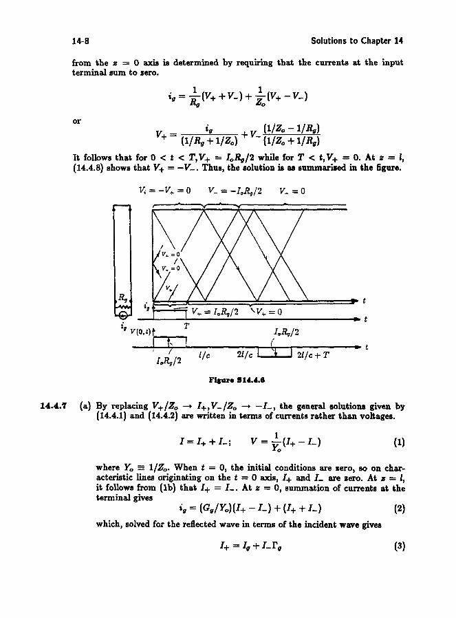SOLUTIONS TO CHAPTER 14

141 DISTRIBUTED PARAMETER EQUIVALENTS AND MODELS

1411 The fields are approximated as uniform in each of the dielectric regions The integral of E between the electrodes must equal the applied voltage and D is conshytinuous at the interface Thus

(1)

and it follows that V

Ea =------------------shy[a + b(euroaeurob)]

(2)

so that the charge per unit length on the upper electrodes is

(3)

where C is the desired capacitance per unit length Because the permeability of the region is uniform H = Iw between the electrodes Thus

gt = (a + b)JLoH = LI L == JLo(a + b)w (4)

where L is the inductance per unit length Note that LC t JLeuro (which permittivity) unless euroa = eurobmiddot

1412 The currents at the node must sum to zero with that through the inductor related to the voltage by V = Ldiconductordt

L a Dz at [I(z) - I(z + Dz)] = V (1)

and C times the rate of change of the voltage drop across the capacitor must be equal to the current through the capacitor

C a Dz at [V(z) - V(z + Dz)] = I (2)

In the limit where Dz - 0 these become the given backward-wave transmission line equations

142 TRANSVERSE ELECTROMAGNETIC WAVES

1



H = 121ff (1)


H = _- aaA



Er = )f21tEr (3)





L == = A(b) - A(a) = IJo In(ab) (5) 1 1 21t


0== A = 21tE (6)V In(ab)




Zo= ~ln(ab)21t




Zo = [iln(21R)fr

and solved for 1R




v

I

1434

Figure 81488


VI = Vo exp(- z2 2a2) 2



J + exp[-(z + ct)22a2]




(1)








V_ =V+


V+ =0



II

Vj ~ V

1 = 0

V+ =0

VI

1442

J = -V2Z

Figure 81441


1 == V2Z

II

V == V2

V=Oj

I == vz


Figure 81442




V+ =Vo2 V_ = -Vo2


V_ = -V+


V+ =0



V =V+ I=V+Zo


1444

bull t

21lclie

Figure 81444

~---~-------------- t

z





-Ra+Rb -Ra+Rb


t

v =0

1_ =0

+ shy

= (R - Ro)12 (P Ro)

z = 1R - Ro)

- 2 (R Ro)

11 1(t)__---I- -- ~ t

I

d1(01)

1~ ~-L~____ I____ 1 t=J

z

I fR - R)TIR R


Figure 81-amp45



or


i g (lZo - 1Rg )

V+ = (1Rg + lZo) + V_ (lZo + 1Rg )


v=-v+=o

z~ ft=lt==============Pbulli

g V(o t)t IoRg2


-e-+-

T-- t

I~2 le

Fleur 81448


1V=Y

o(I+-L) (1)


i g = (Gg jYo)(l+ - L) + (1+ + L)


(2)

(3)


where

14-9

(4)


(5)

+

4 N=

iDLt


2 3

Figure 81447


(r N

-1

)1(0 t) =10 1 - (1 + oOg) (6)


i g = lLOg ~~ + I


1(0 t) =10 (1 - e-tT ) l == lLOg

(7)

(8)



(9)

Thus

I 2Nl2(N-l)- lttlt-

c c(10)


I I2(N - 1)- lt t lt 2N-

c c(11)


1448

lie

-2J__f_v_o---1-7 _

1 V (0 ) (10) = V = V12 ~voVo21 -------hl-


z~

+ V g -

Figure 91448




OL(RL + Zo) ~ + V_ = ~o U-l(t - llc)






Y(81 = -112) Yo Yo Yo = YL = jwOL


Z(81 = -112) Zo Zo = jwLL



Y(-l) 1- rLe-21I 1- e-2i~1

---y-- = 1 +r Le-2i~1 = 1+ e-2i~1


Y(-l) -- =jtan81

Yo




v=v+ exp(-j8Z)j

z



Figure 81411















V+ = ~o sin[B(z + l)]





I 1 1 2 - j2 r+ JX =

=-1 rL + JXL 2+ j2 8



















Z = Zo = (R + iwL) = 1 i81 -821 [G + iwCl1






Z -+ Zoi81 = I(R + iwL)










Thus

(3)




Thus

dtT


~ ~ ~ di]+ jwCVV - V ---J dz

0 1 dt dl = - -Re [1- + tT-]dz (6)

_12 dz dz







ot ot ot2



OZ ot


01 oVL- = -JjuV - LC- (3)

OZ ot

From (8614) and (764)

(4)

Thus











E = - Bqgtix

_ BqgtiBx By Y

where


qgt - -Re - e3



where







Bz Bz Bt



4 z t

(2)

(3)



(4)






Eb Eb t





1491 From (14911) 2

R=-shy1rWU










1 lt In[( i) + Y(Ia)2 - 1]a



1492 From (14911)

1 1 1 1 1 R = 027la~ + 07lb2 = frO [a~ + b2 ]



In(ab)








1 In(ab) -lt [a~ + ](b2and~2)






n=l





H = 121ff (1)


H = _- aaA



Er = )f21tEr (3)





L == = A(b) - A(a) = IJo In(ab) (5) 1 1 21t


0== A = 21tE (6)V In(ab)




Zo= ~ln(ab)21t




Zo = [iln(21R)fr

and solved for 1R




v

I

1434

Figure 81488


VI = Vo exp(- z2 2a2) 2



J + exp[-(z + ct)22a2]




(1)








V_ =V+


V+ =0



II

Vj ~ V

1 = 0

V+ =0

VI

1442

J = -V2Z

Figure 81441


1 == V2Z

II

V == V2

V=Oj

I == vz


Figure 81442




V+ =Vo2 V_ = -Vo2


V_ = -V+


V+ =0



V =V+ I=V+Zo


1444

bull t

21lclie

Figure 81444

~---~-------------- t

z





-Ra+Rb -Ra+Rb


t

v =0

1_ =0

+ shy

= (R - Ro)12 (P Ro)

z = 1R - Ro)

- 2 (R Ro)

11 1(t)__---I- -- ~ t

I

d1(01)

1~ ~-L~____ I____ 1 t=J

z

I fR - R)TIR R


Figure 81-amp45



or


i g (lZo - 1Rg )

V+ = (1Rg + lZo) + V_ (lZo + 1Rg )


v=-v+=o

z~ ft=lt==============Pbulli

g V(o t)t IoRg2


-e-+-

T-- t

I~2 le

Fleur 81448


1V=Y

o(I+-L) (1)


i g = (Gg jYo)(l+ - L) + (1+ + L)


(2)

(3)


where

14-9

(4)


(5)

+

4 N=

iDLt


2 3

Figure 81447


(r N

-1

)1(0 t) =10 1 - (1 + oOg) (6)


i g = lLOg ~~ + I


1(0 t) =10 (1 - e-tT ) l == lLOg

(7)

(8)



(9)

Thus

I 2Nl2(N-l)- lttlt-

c c(10)


I I2(N - 1)- lt t lt 2N-

c c(11)


1448

lie

-2J__f_v_o---1-7 _

1 V (0 ) (10) = V = V12 ~voVo21 -------hl-


z~

+ V g -

Figure 91448




OL(RL + Zo) ~ + V_ = ~o U-l(t - llc)






Y(81 = -112) Yo Yo Yo = YL = jwOL


Z(81 = -112) Zo Zo = jwLL



Y(-l) 1- rLe-21I 1- e-2i~1

---y-- = 1 +r Le-2i~1 = 1+ e-2i~1


Y(-l) -- =jtan81

Yo




v=v+ exp(-j8Z)j

z



Figure 81411















V+ = ~o sin[B(z + l)]





I 1 1 2 - j2 r+ JX =

=-1 rL + JXL 2+ j2 8



















Z = Zo = (R + iwL) = 1 i81 -821 [G + iwCl1






Z -+ Zoi81 = I(R + iwL)










Thus

(3)




Thus

dtT


~ ~ ~ di]+ jwCVV - V ---J dz

0 1 dt dl = - -Re [1- + tT-]dz (6)

_12 dz dz







ot ot ot2



OZ ot


01 oVL- = -JjuV - LC- (3)

OZ ot

From (8614) and (764)

(4)

Thus











E = - Bqgtix

_ BqgtiBx By Y

where


qgt - -Re - e3



where







Bz Bz Bt



4 z t

(2)

(3)



(4)






Eb Eb t





1491 From (14911) 2

R=-shy1rWU










1 lt In[( i) + Y(Ia)2 - 1]a



1492 From (14911)

1 1 1 1 1 R = 027la~ + 07lb2 = frO [a~ + b2 ]



In(ab)








1 In(ab) -lt [a~ + ](b2and~2)






n=l





Zo = [iln(21R)fr

and solved for 1R




v

I

1434

Figure 81488


VI = Vo exp(- z2 2a2) 2



J + exp[-(z + ct)22a2]




(1)








V_ =V+


V+ =0



II

Vj ~ V

1 = 0

V+ =0

VI

1442

J = -V2Z

Figure 81441


1 == V2Z

II

V == V2

V=Oj

I == vz


Figure 81442




V+ =Vo2 V_ = -Vo2


V_ = -V+


V+ =0



V =V+ I=V+Zo


1444

bull t

21lclie

Figure 81444

~---~-------------- t

z





-Ra+Rb -Ra+Rb


t

v =0

1_ =0

+ shy

= (R - Ro)12 (P Ro)

z = 1R - Ro)

- 2 (R Ro)

11 1(t)__---I- -- ~ t

I

d1(01)

1~ ~-L~____ I____ 1 t=J

z

I fR - R)TIR R


Figure 81-amp45



or


i g (lZo - 1Rg )

V+ = (1Rg + lZo) + V_ (lZo + 1Rg )


v=-v+=o

z~ ft=lt==============Pbulli

g V(o t)t IoRg2


-e-+-

T-- t

I~2 le

Fleur 81448


1V=Y

o(I+-L) (1)


i g = (Gg jYo)(l+ - L) + (1+ + L)


(2)

(3)


where

14-9

(4)


(5)

+

4 N=

iDLt


2 3

Figure 81447


(r N

-1

)1(0 t) =10 1 - (1 + oOg) (6)


i g = lLOg ~~ + I


1(0 t) =10 (1 - e-tT ) l == lLOg

(7)

(8)



(9)

Thus

I 2Nl2(N-l)- lttlt-

c c(10)


I I2(N - 1)- lt t lt 2N-

c c(11)


1448

lie

-2J__f_v_o---1-7 _

1 V (0 ) (10) = V = V12 ~voVo21 -------hl-


z~

+ V g -

Figure 91448




OL(RL + Zo) ~ + V_ = ~o U-l(t - llc)






Y(81 = -112) Yo Yo Yo = YL = jwOL


Z(81 = -112) Zo Zo = jwLL



Y(-l) 1- rLe-21I 1- e-2i~1

---y-- = 1 +r Le-2i~1 = 1+ e-2i~1


Y(-l) -- =jtan81

Yo




v=v+ exp(-j8Z)j

z



Figure 81411















V+ = ~o sin[B(z + l)]





I 1 1 2 - j2 r+ JX =

=-1 rL + JXL 2+ j2 8



















Z = Zo = (R + iwL) = 1 i81 -821 [G + iwCl1






Z -+ Zoi81 = I(R + iwL)










Thus

(3)




Thus

dtT


~ ~ ~ di]+ jwCVV - V ---J dz

0 1 dt dl = - -Re [1- + tT-]dz (6)

_12 dz dz







ot ot ot2



OZ ot


01 oVL- = -JjuV - LC- (3)

OZ ot

From (8614) and (764)

(4)

Thus











E = - Bqgtix

_ BqgtiBx By Y

where


qgt - -Re - e3



where







Bz Bz Bt



4 z t

(2)

(3)



(4)






Eb Eb t





1491 From (14911) 2

R=-shy1rWU










1 lt In[( i) + Y(Ia)2 - 1]a



1492 From (14911)

1 1 1 1 1 R = 027la~ + 07lb2 = frO [a~ + b2 ]



In(ab)








1 In(ab) -lt [a~ + ](b2and~2)






n=l






(1)








V_ =V+


V+ =0



II

Vj ~ V

1 = 0

V+ =0

VI

1442

J = -V2Z

Figure 81441


1 == V2Z

II

V == V2

V=Oj

I == vz


Figure 81442




V+ =Vo2 V_ = -Vo2


V_ = -V+


V+ =0



V =V+ I=V+Zo


1444

bull t

21lclie

Figure 81444

~---~-------------- t

z





-Ra+Rb -Ra+Rb


t

v =0

1_ =0

+ shy

= (R - Ro)12 (P Ro)

z = 1R - Ro)

- 2 (R Ro)

11 1(t)__---I- -- ~ t

I

d1(01)

1~ ~-L~____ I____ 1 t=J

z

I fR - R)TIR R


Figure 81-amp45



or


i g (lZo - 1Rg )

V+ = (1Rg + lZo) + V_ (lZo + 1Rg )


v=-v+=o

z~ ft=lt==============Pbulli

g V(o t)t IoRg2


-e-+-

T-- t

I~2 le

Fleur 81448


1V=Y

o(I+-L) (1)


i g = (Gg jYo)(l+ - L) + (1+ + L)


(2)

(3)


where

14-9

(4)


(5)

+

4 N=

iDLt


2 3

Figure 81447


(r N

-1

)1(0 t) =10 1 - (1 + oOg) (6)


i g = lLOg ~~ + I


1(0 t) =10 (1 - e-tT ) l == lLOg

(7)

(8)



(9)

Thus

I 2Nl2(N-l)- lttlt-

c c(10)


I I2(N - 1)- lt t lt 2N-

c c(11)


1448

lie

-2J__f_v_o---1-7 _

1 V (0 ) (10) = V = V12 ~voVo21 -------hl-


z~

+ V g -

Figure 91448




OL(RL + Zo) ~ + V_ = ~o U-l(t - llc)






Y(81 = -112) Yo Yo Yo = YL = jwOL


Z(81 = -112) Zo Zo = jwLL



Y(-l) 1- rLe-21I 1- e-2i~1

---y-- = 1 +r Le-2i~1 = 1+ e-2i~1


Y(-l) -- =jtan81

Yo




v=v+ exp(-j8Z)j

z



Figure 81411















V+ = ~o sin[B(z + l)]





I 1 1 2 - j2 r+ JX =

=-1 rL + JXL 2+ j2 8



















Z = Zo = (R + iwL) = 1 i81 -821 [G + iwCl1






Z -+ Zoi81 = I(R + iwL)










Thus

(3)




Thus

dtT


~ ~ ~ di]+ jwCVV - V ---J dz

0 1 dt dl = - -Re [1- + tT-]dz (6)

_12 dz dz







ot ot ot2



OZ ot


01 oVL- = -JjuV - LC- (3)

OZ ot

From (8614) and (764)

(4)

Thus











E = - Bqgtix

_ BqgtiBx By Y

where


qgt - -Re - e3



where







Bz Bz Bt



4 z t

(2)

(3)



(4)






Eb Eb t





1491 From (14911) 2

R=-shy1rWU










1 lt In[( i) + Y(Ia)2 - 1]a



1492 From (14911)

1 1 1 1 1 R = 027la~ + 07lb2 = frO [a~ + b2 ]



In(ab)








1 In(ab) -lt [a~ + ](b2and~2)






n=l




II

Vj ~ V

1 = 0

V+ =0

VI

1442

J = -V2Z

Figure 81441


1 == V2Z

II

V == V2

V=Oj

I == vz


Figure 81442




V+ =Vo2 V_ = -Vo2


V_ = -V+


V+ =0



V =V+ I=V+Zo


1444

bull t

21lclie

Figure 81444

~---~-------------- t

z





-Ra+Rb -Ra+Rb


t

v =0

1_ =0

+ shy

= (R - Ro)12 (P Ro)

z = 1R - Ro)

- 2 (R Ro)

11 1(t)__---I- -- ~ t

I

d1(01)

1~ ~-L~____ I____ 1 t=J

z

I fR - R)TIR R


Figure 81-amp45



or


i g (lZo - 1Rg )

V+ = (1Rg + lZo) + V_ (lZo + 1Rg )


v=-v+=o

z~ ft=lt==============Pbulli

g V(o t)t IoRg2


-e-+-

T-- t

I~2 le

Fleur 81448


1V=Y

o(I+-L) (1)


i g = (Gg jYo)(l+ - L) + (1+ + L)


(2)

(3)


where

14-9

(4)


(5)

+

4 N=

iDLt


2 3

Figure 81447


(r N

-1

)1(0 t) =10 1 - (1 + oOg) (6)


i g = lLOg ~~ + I


1(0 t) =10 (1 - e-tT ) l == lLOg

(7)

(8)



(9)

Thus

I 2Nl2(N-l)- lttlt-

c c(10)


I I2(N - 1)- lt t lt 2N-

c c(11)


1448

lie

-2J__f_v_o---1-7 _

1 V (0 ) (10) = V = V12 ~voVo21 -------hl-


z~

+ V g -

Figure 91448




OL(RL + Zo) ~ + V_ = ~o U-l(t - llc)






Y(81 = -112) Yo Yo Yo = YL = jwOL


Z(81 = -112) Zo Zo = jwLL



Y(-l) 1- rLe-21I 1- e-2i~1

---y-- = 1 +r Le-2i~1 = 1+ e-2i~1


Y(-l) -- =jtan81

Yo




v=v+ exp(-j8Z)j

z



Figure 81411















V+ = ~o sin[B(z + l)]





I 1 1 2 - j2 r+ JX =

=-1 rL + JXL 2+ j2 8



















Z = Zo = (R + iwL) = 1 i81 -821 [G + iwCl1






Z -+ Zoi81 = I(R + iwL)










Thus

(3)




Thus

dtT


~ ~ ~ di]+ jwCVV - V ---J dz

0 1 dt dl = - -Re [1- + tT-]dz (6)

_12 dz dz







ot ot ot2



OZ ot


01 oVL- = -JjuV - LC- (3)

OZ ot

From (8614) and (764)

(4)

Thus











E = - Bqgtix

_ BqgtiBx By Y

where


qgt - -Re - e3



where







Bz Bz Bt



4 z t

(2)

(3)



(4)






Eb Eb t





1491 From (14911) 2

R=-shy1rWU










1 lt In[( i) + Y(Ia)2 - 1]a



1492 From (14911)

1 1 1 1 1 R = 027la~ + 07lb2 = frO [a~ + b2 ]



In(ab)








1 In(ab) -lt [a~ + ](b2and~2)






n=l





V+ =Vo2 V_ = -Vo2


V_ = -V+


V+ =0



V =V+ I=V+Zo


1444

bull t

21lclie

Figure 81444

~---~-------------- t

z





-Ra+Rb -Ra+Rb


t

v =0

1_ =0

+ shy

= (R - Ro)12 (P Ro)

z = 1R - Ro)

- 2 (R Ro)

11 1(t)__---I- -- ~ t

I

d1(01)

1~ ~-L~____ I____ 1 t=J

z

I fR - R)TIR R


Figure 81-amp45



or


i g (lZo - 1Rg )

V+ = (1Rg + lZo) + V_ (lZo + 1Rg )


v=-v+=o

z~ ft=lt==============Pbulli

g V(o t)t IoRg2


-e-+-

T-- t

I~2 le

Fleur 81448


1V=Y

o(I+-L) (1)


i g = (Gg jYo)(l+ - L) + (1+ + L)


(2)

(3)


where

14-9

(4)


(5)

+

4 N=

iDLt


2 3

Figure 81447


(r N

-1

)1(0 t) =10 1 - (1 + oOg) (6)


i g = lLOg ~~ + I


1(0 t) =10 (1 - e-tT ) l == lLOg

(7)

(8)



(9)

Thus

I 2Nl2(N-l)- lttlt-

c c(10)


I I2(N - 1)- lt t lt 2N-

c c(11)


1448

lie

-2J__f_v_o---1-7 _

1 V (0 ) (10) = V = V12 ~voVo21 -------hl-


z~

+ V g -

Figure 91448




OL(RL + Zo) ~ + V_ = ~o U-l(t - llc)






Y(81 = -112) Yo Yo Yo = YL = jwOL


Z(81 = -112) Zo Zo = jwLL



Y(-l) 1- rLe-21I 1- e-2i~1

---y-- = 1 +r Le-2i~1 = 1+ e-2i~1


Y(-l) -- =jtan81

Yo




v=v+ exp(-j8Z)j

z



Figure 81411















V+ = ~o sin[B(z + l)]





I 1 1 2 - j2 r+ JX =

=-1 rL + JXL 2+ j2 8



















Z = Zo = (R + iwL) = 1 i81 -821 [G + iwCl1






Z -+ Zoi81 = I(R + iwL)










Thus

(3)




Thus

dtT


~ ~ ~ di]+ jwCVV - V ---J dz

0 1 dt dl = - -Re [1- + tT-]dz (6)

_12 dz dz







ot ot ot2



OZ ot


01 oVL- = -JjuV - LC- (3)

OZ ot

From (8614) and (764)

(4)

Thus











E = - Bqgtix

_ BqgtiBx By Y

where


qgt - -Re - e3



where







Bz Bz Bt



4 z t

(2)

(3)



(4)






Eb Eb t





1491 From (14911) 2

R=-shy1rWU










1 lt In[( i) + Y(Ia)2 - 1]a



1492 From (14911)

1 1 1 1 1 R = 027la~ + 07lb2 = frO [a~ + b2 ]



In(ab)








1 In(ab) -lt [a~ + ](b2and~2)






n=l







-Ra+Rb -Ra+Rb


t

v =0

1_ =0

+ shy

= (R - Ro)12 (P Ro)

z = 1R - Ro)

- 2 (R Ro)

11 1(t)__---I- -- ~ t

I

d1(01)

1~ ~-L~____ I____ 1 t=J

z

I fR - R)TIR R


Figure 81-amp45



or


i g (lZo - 1Rg )

V+ = (1Rg + lZo) + V_ (lZo + 1Rg )


v=-v+=o

z~ ft=lt==============Pbulli

g V(o t)t IoRg2


-e-+-

T-- t

I~2 le

Fleur 81448


1V=Y

o(I+-L) (1)


i g = (Gg jYo)(l+ - L) + (1+ + L)


(2)

(3)


where

14-9

(4)


(5)

+

4 N=

iDLt


2 3

Figure 81447


(r N

-1

)1(0 t) =10 1 - (1 + oOg) (6)


i g = lLOg ~~ + I


1(0 t) =10 (1 - e-tT ) l == lLOg

(7)

(8)



(9)

Thus

I 2Nl2(N-l)- lttlt-

c c(10)


I I2(N - 1)- lt t lt 2N-

c c(11)


1448

lie

-2J__f_v_o---1-7 _

1 V (0 ) (10) = V = V12 ~voVo21 -------hl-


z~

+ V g -

Figure 91448




OL(RL + Zo) ~ + V_ = ~o U-l(t - llc)






Y(81 = -112) Yo Yo Yo = YL = jwOL


Z(81 = -112) Zo Zo = jwLL



Y(-l) 1- rLe-21I 1- e-2i~1

---y-- = 1 +r Le-2i~1 = 1+ e-2i~1


Y(-l) -- =jtan81

Yo




v=v+ exp(-j8Z)j

z



Figure 81411















V+ = ~o sin[B(z + l)]





I 1 1 2 - j2 r+ JX =

=-1 rL + JXL 2+ j2 8



















Z = Zo = (R + iwL) = 1 i81 -821 [G + iwCl1






Z -+ Zoi81 = I(R + iwL)










Thus

(3)




Thus

dtT


~ ~ ~ di]+ jwCVV - V ---J dz

0 1 dt dl = - -Re [1- + tT-]dz (6)

_12 dz dz







ot ot ot2



OZ ot


01 oVL- = -JjuV - LC- (3)

OZ ot

From (8614) and (764)

(4)

Thus











E = - Bqgtix

_ BqgtiBx By Y

where


qgt - -Re - e3



where







Bz Bz Bt



4 z t

(2)

(3)



(4)






Eb Eb t





1491 From (14911) 2

R=-shy1rWU










1 lt In[( i) + Y(Ia)2 - 1]a



1492 From (14911)

1 1 1 1 1 R = 027la~ + 07lb2 = frO [a~ + b2 ]



In(ab)








1 In(ab) -lt [a~ + ](b2and~2)






n=l




or


i g (lZo - 1Rg )

V+ = (1Rg + lZo) + V_ (lZo + 1Rg )


v=-v+=o

z~ ft=lt==============Pbulli

g V(o t)t IoRg2


-e-+-

T-- t

I~2 le

Fleur 81448


1V=Y

o(I+-L) (1)


i g = (Gg jYo)(l+ - L) + (1+ + L)


(2)

(3)


where

14-9

(4)


(5)

+

4 N=

iDLt


2 3

Figure 81447


(r N

-1

)1(0 t) =10 1 - (1 + oOg) (6)


i g = lLOg ~~ + I


1(0 t) =10 (1 - e-tT ) l == lLOg

(7)

(8)



(9)

Thus

I 2Nl2(N-l)- lttlt-

c c(10)


I I2(N - 1)- lt t lt 2N-

c c(11)


1448

lie

-2J__f_v_o---1-7 _

1 V (0 ) (10) = V = V12 ~voVo21 -------hl-


z~

+ V g -

Figure 91448




OL(RL + Zo) ~ + V_ = ~o U-l(t - llc)






Y(81 = -112) Yo Yo Yo = YL = jwOL


Z(81 = -112) Zo Zo = jwLL



Y(-l) 1- rLe-21I 1- e-2i~1

---y-- = 1 +r Le-2i~1 = 1+ e-2i~1


Y(-l) -- =jtan81

Yo




v=v+ exp(-j8Z)j

z



Figure 81411















V+ = ~o sin[B(z + l)]





I 1 1 2 - j2 r+ JX =

=-1 rL + JXL 2+ j2 8



















Z = Zo = (R + iwL) = 1 i81 -821 [G + iwCl1






Z -+ Zoi81 = I(R + iwL)










Thus

(3)




Thus

dtT


~ ~ ~ di]+ jwCVV - V ---J dz

0 1 dt dl = - -Re [1- + tT-]dz (6)

_12 dz dz







ot ot ot2



OZ ot


01 oVL- = -JjuV - LC- (3)

OZ ot

From (8614) and (764)

(4)

Thus











E = - Bqgtix

_ BqgtiBx By Y

where


qgt - -Re - e3



where







Bz Bz Bt



4 z t

(2)

(3)



(4)






Eb Eb t





1491 From (14911) 2

R=-shy1rWU










1 lt In[( i) + Y(Ia)2 - 1]a



1492 From (14911)

1 1 1 1 1 R = 027la~ + 07lb2 = frO [a~ + b2 ]



In(ab)








1 In(ab) -lt [a~ + ](b2and~2)






n=l




where

14-9

(4)


(5)

+

4 N=

iDLt


2 3

Figure 81447


(r N

-1

)1(0 t) =10 1 - (1 + oOg) (6)


i g = lLOg ~~ + I


1(0 t) =10 (1 - e-tT ) l == lLOg

(7)

(8)



(9)

Thus

I 2Nl2(N-l)- lttlt-

c c(10)


I I2(N - 1)- lt t lt 2N-

c c(11)


1448

lie

-2J__f_v_o---1-7 _

1 V (0 ) (10) = V = V12 ~voVo21 -------hl-


z~

+ V g -

Figure 91448




OL(RL + Zo) ~ + V_ = ~o U-l(t - llc)






Y(81 = -112) Yo Yo Yo = YL = jwOL


Z(81 = -112) Zo Zo = jwLL



Y(-l) 1- rLe-21I 1- e-2i~1

---y-- = 1 +r Le-2i~1 = 1+ e-2i~1


Y(-l) -- =jtan81

Yo




v=v+ exp(-j8Z)j

z



Figure 81411















V+ = ~o sin[B(z + l)]





I 1 1 2 - j2 r+ JX =

=-1 rL + JXL 2+ j2 8



















Z = Zo = (R + iwL) = 1 i81 -821 [G + iwCl1






Z -+ Zoi81 = I(R + iwL)










Thus

(3)




Thus

dtT


~ ~ ~ di]+ jwCVV - V ---J dz

0 1 dt dl = - -Re [1- + tT-]dz (6)

_12 dz dz







ot ot ot2



OZ ot


01 oVL- = -JjuV - LC- (3)

OZ ot

From (8614) and (764)

(4)

Thus











E = - Bqgtix

_ BqgtiBx By Y

where


qgt - -Re - e3



where







Bz Bz Bt



4 z t

(2)

(3)



(4)






Eb Eb t





1491 From (14911) 2

R=-shy1rWU










1 lt In[( i) + Y(Ia)2 - 1]a



1492 From (14911)

1 1 1 1 1 R = 027la~ + 07lb2 = frO [a~ + b2 ]



In(ab)








1 In(ab) -lt [a~ + ](b2and~2)






n=l





(9)

Thus

I 2Nl2(N-l)- lttlt-

c c(10)


I I2(N - 1)- lt t lt 2N-

c c(11)


1448

lie

-2J__f_v_o---1-7 _

1 V (0 ) (10) = V = V12 ~voVo21 -------hl-


z~

+ V g -

Figure 91448




OL(RL + Zo) ~ + V_ = ~o U-l(t - llc)






Y(81 = -112) Yo Yo Yo = YL = jwOL


Z(81 = -112) Zo Zo = jwLL



Y(-l) 1- rLe-21I 1- e-2i~1

---y-- = 1 +r Le-2i~1 = 1+ e-2i~1


Y(-l) -- =jtan81

Yo




v=v+ exp(-j8Z)j

z



Figure 81411















V+ = ~o sin[B(z + l)]





I 1 1 2 - j2 r+ JX =

=-1 rL + JXL 2+ j2 8



















Z = Zo = (R + iwL) = 1 i81 -821 [G + iwCl1






Z -+ Zoi81 = I(R + iwL)










Thus

(3)




Thus

dtT


~ ~ ~ di]+ jwCVV - V ---J dz

0 1 dt dl = - -Re [1- + tT-]dz (6)

_12 dz dz







ot ot ot2



OZ ot


01 oVL- = -JjuV - LC- (3)

OZ ot

From (8614) and (764)

(4)

Thus











E = - Bqgtix

_ BqgtiBx By Y

where


qgt - -Re - e3



where







Bz Bz Bt



4 z t

(2)

(3)



(4)






Eb Eb t





1491 From (14911) 2

R=-shy1rWU










1 lt In[( i) + Y(Ia)2 - 1]a



1492 From (14911)

1 1 1 1 1 R = 027la~ + 07lb2 = frO [a~ + b2 ]



In(ab)








1 In(ab) -lt [a~ + ](b2and~2)






n=l





OL(RL + Zo) ~ + V_ = ~o U-l(t - llc)






Y(81 = -112) Yo Yo Yo = YL = jwOL


Z(81 = -112) Zo Zo = jwLL



Y(-l) 1- rLe-21I 1- e-2i~1

---y-- = 1 +r Le-2i~1 = 1+ e-2i~1


Y(-l) -- =jtan81

Yo




v=v+ exp(-j8Z)j

z



Figure 81411















V+ = ~o sin[B(z + l)]





I 1 1 2 - j2 r+ JX =

=-1 rL + JXL 2+ j2 8



















Z = Zo = (R + iwL) = 1 i81 -821 [G + iwCl1






Z -+ Zoi81 = I(R + iwL)










Thus

(3)




Thus

dtT


~ ~ ~ di]+ jwCVV - V ---J dz

0 1 dt dl = - -Re [1- + tT-]dz (6)

_12 dz dz







ot ot ot2



OZ ot


01 oVL- = -JjuV - LC- (3)

OZ ot

From (8614) and (764)

(4)

Thus











E = - Bqgtix

_ BqgtiBx By Y

where


qgt - -Re - e3



where







Bz Bz Bt



4 z t

(2)

(3)



(4)






Eb Eb t





1491 From (14911) 2

R=-shy1rWU










1 lt In[( i) + Y(Ia)2 - 1]a



1492 From (14911)

1 1 1 1 1 R = 027la~ + 07lb2 = frO [a~ + b2 ]



In(ab)








1 In(ab) -lt [a~ + ](b2and~2)






n=l





v=v+ exp(-j8Z)j

z



Figure 81411















V+ = ~o sin[B(z + l)]





I 1 1 2 - j2 r+ JX =

=-1 rL + JXL 2+ j2 8



















Z = Zo = (R + iwL) = 1 i81 -821 [G + iwCl1






Z -+ Zoi81 = I(R + iwL)










Thus

(3)




Thus

dtT


~ ~ ~ di]+ jwCVV - V ---J dz

0 1 dt dl = - -Re [1- + tT-]dz (6)

_12 dz dz







ot ot ot2



OZ ot


01 oVL- = -JjuV - LC- (3)

OZ ot

From (8614) and (764)

(4)

Thus











E = - Bqgtix

_ BqgtiBx By Y

where


qgt - -Re - e3



where







Bz Bz Bt



4 z t

(2)

(3)



(4)






Eb Eb t





1491 From (14911) 2

R=-shy1rWU










1 lt In[( i) + Y(Ia)2 - 1]a



1492 From (14911)

1 1 1 1 1 R = 027la~ + 07lb2 = frO [a~ + b2 ]



In(ab)








1 In(ab) -lt [a~ + ](b2and~2)






n=l









V+ = ~o sin[B(z + l)]





I 1 1 2 - j2 r+ JX =

=-1 rL + JXL 2+ j2 8



















Z = Zo = (R + iwL) = 1 i81 -821 [G + iwCl1






Z -+ Zoi81 = I(R + iwL)










Thus

(3)




Thus

dtT


~ ~ ~ di]+ jwCVV - V ---J dz

0 1 dt dl = - -Re [1- + tT-]dz (6)

_12 dz dz







ot ot ot2



OZ ot


01 oVL- = -JjuV - LC- (3)

OZ ot

From (8614) and (764)

(4)

Thus











E = - Bqgtix

_ BqgtiBx By Y

where


qgt - -Re - e3



where







Bz Bz Bt



4 z t

(2)

(3)



(4)






Eb Eb t





1491 From (14911) 2

R=-shy1rWU










1 lt In[( i) + Y(Ia)2 - 1]a



1492 From (14911)

1 1 1 1 1 R = 027la~ + 07lb2 = frO [a~ + b2 ]



In(ab)








1 In(ab) -lt [a~ + ](b2and~2)






n=l




















Z = Zo = (R + iwL) = 1 i81 -821 [G + iwCl1






Z -+ Zoi81 = I(R + iwL)










Thus

(3)




Thus

dtT


~ ~ ~ di]+ jwCVV - V ---J dz

0 1 dt dl = - -Re [1- + tT-]dz (6)

_12 dz dz







ot ot ot2



OZ ot


01 oVL- = -JjuV - LC- (3)

OZ ot

From (8614) and (764)

(4)

Thus











E = - Bqgtix

_ BqgtiBx By Y

where


qgt - -Re - e3



where







Bz Bz Bt



4 z t

(2)

(3)



(4)






Eb Eb t





1491 From (14911) 2

R=-shy1rWU










1 lt In[( i) + Y(Ia)2 - 1]a



1492 From (14911)

1 1 1 1 1 R = 027la~ + 07lb2 = frO [a~ + b2 ]



In(ab)








1 In(ab) -lt [a~ + ](b2and~2)






n=l








Thus

(3)




Thus

dtT


~ ~ ~ di]+ jwCVV - V ---J dz

0 1 dt dl = - -Re [1- + tT-]dz (6)

_12 dz dz







ot ot ot2



OZ ot


01 oVL- = -JjuV - LC- (3)

OZ ot

From (8614) and (764)

(4)

Thus











E = - Bqgtix

_ BqgtiBx By Y

where


qgt - -Re - e3



where







Bz Bz Bt



4 z t

(2)

(3)



(4)






Eb Eb t





1491 From (14911) 2

R=-shy1rWU










1 lt In[( i) + Y(Ia)2 - 1]a



1492 From (14911)

1 1 1 1 1 R = 027la~ + 07lb2 = frO [a~ + b2 ]



In(ab)








1 In(ab) -lt [a~ + ](b2and~2)






n=l






ot ot ot2



OZ ot


01 oVL- = -JjuV - LC- (3)

OZ ot

From (8614) and (764)

(4)

Thus











E = - Bqgtix

_ BqgtiBx By Y

where


qgt - -Re - e3



where







Bz Bz Bt



4 z t

(2)

(3)



(4)






Eb Eb t





1491 From (14911) 2

R=-shy1rWU










1 lt In[( i) + Y(Ia)2 - 1]a



1492 From (14911)

1 1 1 1 1 R = 027la~ + 07lb2 = frO [a~ + b2 ]



In(ab)








1 In(ab) -lt [a~ + ](b2and~2)






n=l





E = - Bqgtix

_ BqgtiBx By Y

where


qgt - -Re - e3



where







Bz Bz Bt



4 z t

(2)

(3)



(4)






Eb Eb t





1491 From (14911) 2

R=-shy1rWU










1 lt In[( i) + Y(Ia)2 - 1]a



1492 From (14911)

1 1 1 1 1 R = 027la~ + 07lb2 = frO [a~ + b2 ]



In(ab)








1 In(ab) -lt [a~ + ](b2and~2)






n=l








Eb Eb t





1491 From (14911) 2

R=-shy1rWU










1 lt In[( i) + Y(Ia)2 - 1]a



1492 From (14911)

1 1 1 1 1 R = 027la~ + 07lb2 = frO [a~ + b2 ]



In(ab)








1 In(ab) -lt [a~ + ](b2and~2)






n=l




1492 From (14911)

1 1 1 1 1 R = 027la~ + 07lb2 = frO [a~ + b2 ]



In(ab)








1 In(ab) -lt [a~ + ](b2and~2)






n=l



mit opencourseware haus, hermann a., and james … · haus, hermann a., and james r. melcher....

Documents