December 2003 • NREL/TP-500-35172

Mitigation of Wind Turbine/Vortex Interaction Using Disturbance Accommodating Control

M. Maureen Hand

National Renewable Energy Laboratory 1617 Cole Boulevard Golden, Colorado 80401-3393 NREL is a U.S. Department of Energy LaboratoryOperated by Midwest Research Institute • Battelle

Contract No. DE-AC36-99-GO10337

December 2003 • NREL/TP-500-35172

Mitigation of Wind Turbine/Vortex Interaction Using Disturbance Accommodating Control

M. Maureen Hand Prepared under Task No. WER3.1940

National Renewable Energy Laboratory 1617 Cole Boulevard Golden, Colorado 80401-3393 NREL is a U.S. Department of Energy LaboratoryOperated by Midwest Research Institute • Battelle

Contract No. DE-AC36-99-GO10337

NOTICE

This report was prepared as an account of work sponsored by an agency of the United States government. Neither the United States government nor any agency thereof, nor any of their employees, makes any warranty, express or implied, or assumes any legal liability or responsibility for the accuracy, completeness, or usefulness of any information, apparatus, product, or process disclosed, or represents that its use would not infringe privately owned rights. Reference herein to any specific commercial product, process, or service by trade name, trademark, manufacturer, or otherwise does not necessarily constitute or imply its endorsement, recommendation, or favoring by the United States government or any agency thereof. The views and opinions of authors expressed herein do not necessarily state or reflect those of the United States government or any agency thereof.

Available electronically at http://www.osti.gov/bridge

Available for a processing fee to U.S. Department of Energy and its contractors, in paper, from:

U.S. Department of Energy Office of Scientific and Technical Information P.O. Box 62 Oak Ridge, TN 37831-0062 phone: 865.576.8401 fax: 865.576.5728 email: reports@adonis.osti.gov

Available for sale to the public, in paper, from: U.S. Department of Commerce National Technical Information Service 5285 Port Royal Road Springfield, VA 22161 phone: 800.553.6847 fax: 703.605.6900 email: orders@ntis.fedworld.gov online ordering: http://www.ntis.gov/ordering.htm

Printed on paper containing at least 50% wastepaper, including 20% postconsumer waste

iii

Abstract Wind turbines, a competitive source of emission-free electricity, are being designed with diameters and hub heights approaching 100 m, to further reduce the cost of the energy they produce. At this height above the ground, the wind turbine is exposed to atmospheric phenomena such as low-level jets, gravity waves, and Kelvin-Helmholtz instabilities, which are not currently modeled in wind turbine design codes. These atmospheric phenomena can generate coherent turbulence that causes high cyclic loads on wind turbine blades. These fluctuating loads lead to fatigue damage accumulation and blade lifetime reduction.

The National Renewable Energy Laboratory (NREL) conducted an experiment to record wind turbine load response and inflow measurements. The spatial resolution of the inflow measurements was insufficient to identify specific turbulence characteristics that contribute to high cyclic loads. However, strong evidence supported the hypothesis that coherent vorticity passage through the rotor was directly correlated with large blade cyclic amplitudes.

An analytic Rankine vortex model was created and implemented in wind turbine simulation codes to isolate the aerodynamic response of the wind turbine to inflow vortices. Numerous simulations computed the blade load cyclic response to vortices of varying radius, circulation strength, orientation, location with respect to the hub, and plane of rotation. The vortex in the plane of rotation most likely to occur as a result of Kelvin-Helmholtz instabilities produces the highest cyclic amplitudes. The response is similar for two- and three-blade wind turbines.

Advanced control was used to mitigate vortex-induced blade cyclic loading. The MATLAB© with Simulink© computational environment was used for control design. Disturbance Accommodating Control (DAC) was used to cancel the vortex “disturbance.” Compared to a standard proportional-integral controller, the DAC controller reduced the blade fatigue load for vortices of various sizes and for vortices superimposed on turbulent flow fields. A full-state feedback controller that incorporates more detailed vortex inputs achieved significantly greater blade load reduction. Blade loads attributed to vortex passage, then, can be reduced through advanced control, and further reductions appear feasible.

iv

Acknowledgments Several of my colleagues at the National Wind Technology Center offered assistance that greatly relieved the computational burden associated with this project. Marshall Buhl provided me with a gateway into the AeroDyn code for the analytic vortex model and supplied WT_Perf results for the design of the baseline controller. Jason Cotrell adapted and verified the FAST wind turbine models. Karl Stol answered numerous questions and requests about the implementation and operation of the SymDyn code. Alan Wright furnished necessary counsel about the relation of disturbance models to the wind turbine dynamics codes. Katie Johnson and Lee Jay Fingersh answered all my questions about the mechanics of the control system on the wind turbine. Working with Neil Kelley, whose pioneering work motivated this investigation into the wind turbine/vortex interaction, has been an enlightening experience because of his depth of knowledge of the atmospheric boundary layer. Finally, Mark Balas, at the University of Colorado, provided tremendous guidance and insight into the control design studies.

v

Contents FIGURES.................................................................................................................................................VII EXHIBITS .................................................................................................................................................. X TABLES.....................................................................................................................................................XI ACRONYMS AND ABBREVIATIONS............................................................................................. XIII SYMBOLS..............................................................................................................................................XIV

SUBSCRIPTS........................................................................................................................................ XVIII SUPERSCRIPTS.................................................................................................................................... XVIII

CHAPTER 1................................................................................................................................................ 1 INTRODUCTION....................................................................................................................................... 1

WIND TURBINE OPERATION...................................................................................................................... 3 RESULTS SUMMARY................................................................................................................................... 5

CHAPTER 2................................................................................................................................................ 7 TURBULENCE AND WIND TURBINES ............................................................................................... 7 CHAPTER 3.............................................................................................................................................. 11 EXPERIMENTAL EVALUATION OF TURBULENCE/ROTOR INTERACTION ....................... 11

EXPERIMENTAL DATA..............................................................................................................................11 CORRELATION OF BLADE LOADS AND TURBULENCE..............................................................................13 SPATIAL VARIATION OF TURBULENCE STRUCTURES ..............................................................................19 CHAPTER CONCLUSIONS..........................................................................................................................21

CHAPTER 4.............................................................................................................................................. 22 ANALYTIC VORTEX/ROTOR INTERACTION................................................................................ 22

RANKINE VORTEX MODEL.......................................................................................................................22 VALIDATION WITH EXPERIMENTAL DATA...............................................................................................24 WIND TURBINE SIMULATION...................................................................................................................27 WIND TURBINE RESPONSE TO VORTEX ...................................................................................................28 CHAPTER CONCLUSIONS..........................................................................................................................34

CHAPTER 5.............................................................................................................................................. 36 LOAD MITIGATION THROUGH ADVANCED CONTROL ........................................................... 36

BASELINE PI CONTROLLER......................................................................................................................36 DAC DESIGN METHODOLOGY.................................................................................................................40

Linearized Wind Turbine Model ......................................................................................................... 40 Disturbance Waveform Generator...................................................................................................... 42 Composite (Plant/Disturbance) State Estimator................................................................................. 43 Control Law for DAC.......................................................................................................................... 43 Performance Assessment Criteria....................................................................................................... 44

DAC DESIGNS..........................................................................................................................................46 Ten-Blade Element Disturbance Model .............................................................................................. 46 DAC with Hub-Height Wind Speed Disturbance Model..................................................................... 50 DAC with One-Blade Element Disturbance Model ............................................................................ 53

vi

DAC with Hub-Height Wind Speed and Sinusoidal Vertical Shear Disturbance Model.................... 56 Robustness of DAC HH+VSHR Controller ........................................................................................ 64

CHAPTER CONCLUSIONS..........................................................................................................................67 CHAPTER 6.............................................................................................................................................. 68 CONCLUSION TO THIS WORK AND BEGINNING OF FUTURE INVESTIGATION............... 68 REFERENCES.......................................................................................................................................... 70 APPENDIX A............................................................................................................................................ 73 VORTEX FLOW-FIELD MODEL DERIVATION AND IMPLEMENTATION............................. 73

VORTEX SUPERIMPOSED ON TURBULENT WIND FIELD...........................................................................76 FORTRAN CODE FOR VORTEX CALCULATIONS AND SAMPLE INPUT FILE............................................78

APPENDIX B ............................................................................................................................................ 88 WIND TURBINE SIMULATION CODE INPUT FILES .................................................................... 88

AERODYN INPUT FILES............................................................................................................................88 SYMDYN INPUT FILES..............................................................................................................................89 FAST INPUT FILE.....................................................................................................................................94

APPENDIX C............................................................................................................................................ 98 LINEAR WIND TURBINE MODELS FOR CONTROL DESIGN .................................................... 98

LINEARIZED 4-DEGREE-OF-FREEDOM MODEL ........................................................................................98 FSFB OF 10-ELEMENT DISTURBANCE MODEL........................................................................................98 DAC WITH HUB-HEIGHT WIND SPEED DISTURBANCE MODEL ............................................................102 DAC WITH ONE-ELEMENT DISTURBANCE MODEL ...............................................................................103 DAC WITH HUB-HEIGHT UNIFORM WIND SPEED AND SINUSOIDAL VERTICAL SHEAR DISTURBANCE MODEL ...................................................................................................................................................106

vii

Figures Figure 1-1. Growth trend for wind turbines .................................................................................2

Figure 1-2. Variable-speed wind turbine power capture as a function of tip speed ratio ............4

Figure 1-3. Comparison of constant-speed and variable-speed wind turbine power capture as a function of wind speed ...........................................................................................5

Figure 2-1. Low-level jet height versus speed derived from National Oceanic and Atmospheric Association/Environmental Technology Laboratory (NOAA/ETL) lidar observations obtained over South-Central Kansas....................................................8

Figure 2-2. Diurnal variation of nuisance faults from September 1999 through August 2000 (DOE/EPRI 2000) .....................................................................................................9

Figure 3-1. NWTC inflow measurement array upwind of ART, looking toward prevailing wind direction..........................................................................................................12

Figure 3-2. Schematic of inflow measurement array instrumentation relative to wind turbine rotor position...............................................................................................13

Figure 3-3. Ten-minute average, hub-height, wind speed as a function of atmospheric stability, Ri ..............................................................................................................14

Figure 3-4. Blade root flap bending moment equivalent fatigue load as a function of atmospheric stability, Ri ..........................................................................................15

Figure 3-5. Top 2% blade flap equivalent fatigue load in relation to balance of database (inflow parameters represent 10-minute mean values from hub-height anemometer)............................................................................................................16

Figure 3-6. Ten-minute record showing turbulent events and turbine response (data collected on February 5, 2001, at 0605 Coordinated Universal Time [UTC])........17

Figure 3-7. Histogram of equivalent fatigue load population ....................................................18

Figure 3-8. Spatial variation of turbulence structure and vertical flux of total TKE (data collected December 19, 2000, at 0900 UTC)..........................................................19

Figure 3-9. Another example of spatial variation of turbulence structure and vertical flux of total TKE (data collected February 5, 2001, at 0605 UTC) ................................20

Figure 4-1. Wind turbine coordinate system with counterclockwise rotating vortex of radius R in the XZ plane. The vortex convects to the left by adjusting xo by ∞V *∆t at each simulation time step. .......................................................................................23

viii

Figure 4-2. Wind turbine coordinate system with counterclockwise rotating vortex of radius R in the YZ plane. The vortex convects to the left by adjusting yo by ∞V *∆t at each simulation time step. .......................................................................................23

Figure 4-3. Vortex rotating counterclockwise in the XZ plane. The vortex radius is 10 m; the circulation strength is –716 m2/s. (a) Quiver plot showing vector magnitude and direction; (b) Streamlines; (c) Horizontal velocity component at the top, center, and bottom of the rotor; (d) Vertical velocity component at the top, center, and bottom of the rotor...................................................................................................24

Figure 4-4. Root flap bending moment ranges from LIST experiment for all wind speed bins and for 10 m/s wind speed bin.........................................................................26

Figure 4-5. Circulation strength measured in YZ plane from LIST experiment for all wind speed bins and for 10 m/s wind speed bin. (CW = clockwise; CC = counterclockwise)....................................................................................................26

Figure 4-6. Peak instantaneous absolute value of vorticity in YZ plane as a function of atmospheric stability, Ri. .........................................................................................27

Figure 4-7. Blade load response to vortices of various size, circulation strength, and center height above hub. The vortex rotates clockwise in the YZ plane with 10 m/s convection speed .....................................................................................................29

Figure 4-8. Blade load response to vortices of various size, circulation strength, and center height above hub. The vortex rotates counterclockwise in the YZ plane with 10 m/s convection speed .........................................................................................29

Figure 4-9. Blade load response to vortices of various size, circulation strength, and center height above hub. The vortex rotates clockwise in the XZ plane with convection speed of 10 m/s........................................................................................................30

Figure 4-10. Time-series traces of root flap bending moment resulting from vortex passage ....................................................................................................................32

Figure 4-11. Comparison root flap bending moment response to vortex flow-field approximations with actual vortex-induced bending moment ................................33

Figure 4-12. Dimensionless bending moment response to vortex parameter variation for two- and three-blade turbines ..........................................................................................34

Figure 5-1. Generator torque versus rotor speed curve for generator torque controller ............37

Figure 5-2. Schematic of wind turbine simulation with PI controller in Simulink environment ............................................................................................................38

Figure 5-3. Wind turbine response to test vortex with PI controller..........................................39

Figure 5-4. Schematic of general DAC design ..........................................................................42

ix

Figure 5-5. Schematic of blade pitch actuators (with slow proportional gain) in Simulink environment.............................................................................................................46

Figure 5-6. Schematic of FSFB controller using 10-element disturbance model in Simulink environment.............................................................................................................48

Figure 5-7. Wind turbine response to test vortex with FSFB of 10-element disturbance model controller ......................................................................................................49

Figure 5-8. Schematic of wind turbine simulation with DAC controller in Simulink environment.............................................................................................................50

Figure 5-9. Wind turbine response to test vortex with DAC HH controller ..............................52

Figure 5-10. Wind turbine response to test vortex with DAC 1 BE controller............................54

Figure 5-11. Wind speed estimate, rotor speed, and rotor speed estimate for DAC 1 BE controller .................................................................................................................55

Figure 5-12. Blade states and state estimates for DAC 1 BE controller ......................................56

Figure 5-13. Blade tip velocity components associated with test vortex .....................................57

Figure 5-14. Wind turbine response to test vortex with DAC HH+VSHR controller .................61

Figure 5-15. Blade states and state estimates for DAC HH+VSHR controller............................62

Figure 5-16. Wind speed estimate, rotor speed, and rotor speed estimate for DAC HH+VSHR controller..............................................................................................63

Figure 5-17. Sinusoidal disturbance estimates for DAC HH+VSHR controller..........................64

Figure A-1. Coordinate system of vortex rotating in XZ plane ..................................................73

x

Exhibits Exhibit A-1. Example SNWIND input file ..................................................................................76

Exhibit A-2. MATLAB© script, combine_turb_vortex.m, which superimposes vortex on full-field turbulence............................................................................................76

Exhibit A-3. USERWIND.FOR subroutine .................................................................................78

Exhibit A-4. Example USERWIND.IPT file ...............................................................................86

Exhibit B-1. AeroDyn input file for three-blade turbine specifying vortex calculation routine as wind input ...............................................................................................88

Exhibit B-2. Example SymDyn inputprops.m file for three-blade turbine ..................................89

Exhibit B-3. Example SymDyn inputsim.m file for three-blade turbine .....................................91

Exhibit B-4. Example FAST input file for two-blade turbine .....................................................94

xi

Tables Table 3-1. Comparison of Turbulence Parameters and Load Indicators for Turbulent

Events .....................................................................................................................18

Table 4-1. Root Flap Bending Moment Response to Vortices of Varied Orientation, Plane of Rotation, and Center Height ...............................................................................31

Table 5-1. Comparison of PI Controller Performance for Two- and Three-Blade Turbines....38

Table 5-2. Comparison of PI Controller and State-Space Controller Performance for Step Wind Input ..............................................................................................................47

Table 5-3. Poles for Open Loop System and Closed Loop System..........................................47

Table 5-4. Comparison of PI Controller and FSFB of 10-Element Disturbance Model Controller Performance for Test Vortex .................................................................48

Table 5-5. Comparison of PI Controller and DAC HH Controller Performance Test Vortex, Full-Field Turbulence, and Vortex Superimposed on Turbulence..........................51

Table 5-6. Comparison of PI Controller and DAC 1 BE Controller Performance for Test Vortex, Full-Field Turbulence, and Vortex Superimposed on Turbulence.............53

Table 5-7. Comparison of PI Controller and DAC HH+VSHR Controller Performance for Test Vortex, Full-Field Turbulence, and Vortex Superimposed on Turbulence .....60

Table 5-8. Additional Comparisons of PI Controller and DAC HH+VSHR Controller Performance for Vortex Superimposed on Full-Field Turbulence..........................65

Table 5-9. Effect of Changing Radius and Circulation Strength of Vortex for DAC HH+VSHR Controller.............................................................................................66

Table 5-10. Effect of Changing Vortex Center Height with Respect to Hub for DAC HH+VSHR Controller.............................................................................................67

Table C-1. State Matrix, A ........................................................................................................98

Table C-2. Control Input Matrix, B ...........................................................................................98

Table C-3. Wind Input Matrix, BD (actually 8 × 60, but presented here sectioned by blade element)...................................................................................................................98

Table C-4. Disturbance Gain Matrix, GD (actually 3 × 60 but presented here sectioned by blade element) .......................................................................................................100

Table C-5. State Gain Matrix, GX............................................................................................101

Table C-6. State Weighting Matrix, Q ....................................................................................102

xii

Table C-7. Input Weighting Matrix, R ....................................................................................102

Table C-8. Wind Input Matrix, BD ..........................................................................................102

Table C-9. Disturbance Gain Matrix, GD. ...............................................................................102

Table C-10. State Estimator Gain, KX .......................................................................................103

Table C-11. State Estimator State Weighting Matrix, QE ........................................................103

Table C-12. Wind Input Matrix, BD, Representing Element 20 ................................................103

Table C-13. Disturbance Gain Matrix, GD. ...............................................................................104

Table C-14. State Gain Matrix, GX............................................................................................104

Table C-15. State Weighting Matrix, Q. ...................................................................................104

Table C-16. Input Weighting Matrix, R. ...................................................................................104

Table C-17. State Estimator Gain, KX .......................................................................................104

Table C-18. Disturbance Estimator Gain, KD............................................................................105

Table C-19. State Estimator State Weighting Matrix, QE ........................................................105

Table C-20. State Estimator Input Weighting Matrix, RE ........................................................105

Table C-21. Wind Input Matrix, BD ..........................................................................................106

Table C-22. Disturbance Gain Matrix, GD ................................................................................106

Table C-23. State Gain Matrix, GX ...........................................................................................106

Table C-24. State Weighting Matrix, Q. ...................................................................................106

Table C-25. Input Weighting Matrix, R. ...................................................................................107

Table C-26. State Estimator Gain Matrix, KX............................................................................107

Table C-27. State Estimator Disturbance Gain Matrix, KD. ......................................................107

Table C-28. State Estimator State Weighting Matrix, QE ........................................................107

Table C-29. State Estimator Input Weighting Matrix, RE ........................................................108

xiii

Acronyms and Abbreviations AIAA American Institute of Aeronautics and Astronautics ART Advanced Research Turbine ASME American Society of Mechanical Engineers CART Controls Advanced Research Turbine COE cost of energy DAC disturbance accommodating control DOE U.S. Department of Energy EPRI Electric Power Research Institute FSFB full-state feedback GPS global positioning system IEA International Energy Agency IMU inertial measurement unit lidar Light Detection And Ranging LIST Long-term Inflow and Structure Test LQR linear quadratic regulator NOAA/ETL National Oceanic and Atmospheric Administration/Environmental Technology

Laboratory NREL National Renewable Energy Laboratory NWTC National Wind Technology Center PE power electronics PI proportional-integral (controller) PID proportional-integral-derivative RFB root flap bending moment RMS root mean square sodar Sonic Detection And Ranging Std. Dev. standard deviation UTC coordinated universal time

xiv

Symbols e , )(te estimator error vector

)(teX estimator state error

)(teD estimator disturbance error

g gravity acceleration, m/s2

h wind turbine hub height, m

i number of cycle counting bins (222)

i unit vector in x-direction

m material constant, exponent for the S-N curve (10 for fiberglass composite material), or vertical wind shear exponent

n number of rain-flow cycles in the ith bin

n unit normal vector

q vector of degrees of freedom, rad

q vector of angular velocities, rad/s

q vector of angular accelerations, rad/s2

r radial distance from vortex center to (x, y, z) position, m

t time

u control input (vector of perturbed blade pitch angles), rad

Du wind/disturbance input

u,v,w wind velocity components corresponding to x, y, z coordinates, respectively, m/s

u', v', w' streamwise, crosswind, and vertical instantaneous component velocities in a right-handed coordinate system where the longitudinal or streamwise wind component is parallel to the mean streamline, m/s

'','','' wvvuwu turbulent Reynolds stress components, (m/s)2

uR radial wind velocity component in cylindrical coordinate system, m/s

uθ angular wind velocity component in cylindrical coordinate system, m/s

)(* tu ideal control law

w’(TKE) vertical flux of turbulence kinetic energy, (m/s)3

x , )(tx state vector

0x initial state vector

x,y,z blade element coordinates in aerodynamic code coordinate system, m

xv

x0, y0, z0 position of vortex center in aerodynamic code coordinate system, m

y , )(ty output vector

Dz , )(tzD disturbance state vector

0Dz initial disturbance vector

zg height above ground level, m

A rotor swept area, or arbitrary area for integration, or time-averaged state matrix, N × N

A combined plant/disturbance state matrix, N+ND × N+ND

A(t) periodic state matrix, N × N

AD amplitude of disturbance generator sinusoid, m/s

B time-averaged control input matrix, N × M

B(t) periodic control input matrix, N × M

BD time-averaged disturbance input matrix, N × ND

BD(t) periodic disturbance input matrix, N × ND

Bo constant for normalization of blade root bending moment, kNm

B+ Moore-Penrose pseudoinverse

C output matrix, dim N × P

C combined plant/disturbance output matrix, N × P+ND

CC counterclockwise rotation

Cq rotor torque coefficient

CP rotor power coefficient

CPMAX peak power coefficient

CW clockwise rotation

)(tE wind transmission vector

F disturbance state matrix, NDS × NDS

Fi amplitude of the ith cycle counting bin, kNm

Fe equivalent fatigue load, kNm

G or Γ vortex circulation strength, m2/s

GX state gain

GD disturbance gain

G combined plant/disturbance gain

G(t) gyroscopic matrix in linear equation of motion

Go constant for normalization of vortex circulation, m2/s

xvi

H(t) control input transmission matrix

I identity matrix

J linear quadratic regulator cost function

JT rotor inertia, kg·m2

KX state estimator gain

KD disturbance estimator gain

K combined plant/disturbance estimator gain

K(t) stiffness matrix in linear equations of motion

L vector of applied loads, function of q , q , W, and φ

M number of control inputs

M(q) mass matrix in nonlinear equations of motion

M(t) mass matrix in linear equations of motion

N number of states

NDOF number of degrees of freedom

NB number of blades

ND number of disturbance inputs

NDS number of disturbance states

No cycles over 10-minute period (840)

P number of plant (turbine) outputs

Q linear quadratic regulator state weighting matrix

QE linear quadratic regulator estimator state weighting matrix

QP dynamic pressure over rotor based on mean convection speed, Pa

QA aerodynamic torque, N·m

QE generator torque, N·m

R radius of vortex, m, or linear quadratic regulator input weighting matrix

RE linear quadratic regulator estimator input weighting matrix

Ri Richardson number

RS radius of circle formed by sonic anemometers, 21 m

RT radius of wind turbine, m

TI turbulence intensity, (%)

TKE turbulence kinetic energy, (m/s)2

)( gzU mean horizontal inflow velocity at height zg

U total wind velocity vector, m/s

xvii

∞V convection speed of vortex, m/s

W wind speed, m/s

α relationship between the perturbed rotor speed and the wind speed perturbation on each blade

αb relationship between the perturbed blade flap angle and the wind speed perturbation on each blade

βj blade flap angle, subscript indicates blade number, rad

φ blade pitch angle, deg

φ vector of blade pitch angles, rad

λ tip speed ratio

λMAX tip speed ratio at peak power coefficient

ρ air density, 1.00 kg/m3 for sea level

σU standard deviation of horizontal wind speed, m/s

Θ disturbance input matrix, ND × NDS

θ angular position in cylindrical coordinate system, rad

mθ mean virtual potential temperature (between 3 m and 61 m), K

)( gv zθ mean virtual potential temperature at height zg, K

ω vorticity, s-1

ψj blade azimuth angle (Blade 1 at 0° in the 12 o’clock position), rad

Ω rotor angular speed, rad/s

∆t simulation time step, 0.004 s

∆ difference between measurements at various zg, or perturbation of state or disturbance

xviii

Subscripts OP operating point

j blade number (1, 2, or 3)

Superscripts x first derivative of x with respect to time, d/dt

x second derivative of x with respect to time, d2/dt2

x estimated value of x

1

Chapter 1

Introduction Recent concern about global climate change has spotlighted renewable energy technologies as emission-free sources of electricity. Wind energy has become the most cost-effective of these technologies, with the cost of wind energy technologies dropping from $0.80/kWh (in 2000 dollars) in 1980 to $0.04–$0.06/kWh in 2000 (IEA 2002). Accompanying these cost reductions and design improvements is the tremendous potential for capacity growth in the U.S. market—at the end of 2002, the installed generating capacity of wind turbines in the United States was 4,685 MW (IEA 2002). The Great Plains region of the country, in particular, has a significant documented resource that is currently being considered for development (Elliot et al. 1987).

The dramatic cost reduction was achieved primarily through the creation of larger machines, which was a direct result of research that improved the analytic tools for design as well as the wind turbine architectures. Improvements to modeling capability and design methodology allowed turbine designers to build larger machines with improved reliability. To continue to reduce the cost of energy (COE), turbine rotor diameters and tower heights will continue to increase. In 2000 the typical commercial wind turbine was rated at 750 kW with a 60 m diameter and a 65 m hub height. In 2003 the “standard size” deployed commercially is 1.5 MW, and new prototypes rated at 5 MW are being tested (as illustrated in Figure 1-1). These turbines will have rotor diameters and hub heights exceeding 100 m (de Vries 2002).

Further reducing the COE without sacrificing structural life or reliability is the design engineer’s challenge. Mass reduction is the primary way to reduce machine cost. Generally the machine’s weight increases with the blade length cubed, while the energy capture increases with the blade length squared (Malcolm and Hansen 2002). Reducing mass for the same power rating has two negative consequences: the design safety margins on critical components are reduced, and the structure becomes more dynamically active. To maximize energy capture and maintain structural integrity, the ability to anticipate the loads the turbine will experience in the operating environment and to mitigate the wind loading through advanced control is critical.

2

Figure 1-1. Growth trend for wind turbines

Most commercial, variable-speed wind turbines use classical proportional-integral-derivative (PID) algorithms to meet a single objective—for example, speed regulation to maintain constant power production in above-rated wind speeds. This type of classical approach to wind turbine control has been demonstrated by a number of researchers (Arsudis and Bohnisch 1990; Leithead et al. 1991; Stuart, Wright, and Butterfield 1996; Hand and Balas 2000). State-space-based design has recently generated a great deal of interest in wind turbine control, primarily because multiple control objectives can be achieved (e.g., speed regulation and blade load reduction). Several researchers have explored state-space-based wind turbine control to meet multiple objectives (Ekelund 1994; Kendall et al. 1997; Balas, Lee and Kendall 1998; Stol, Rigney, and Balas 2000; Stol and Balas 2002; Stol 2003; Wright 2003). These advanced controls, which meet multiple performance objectives, present unique opportunities to balance mass reduction and dampen dynamically excited modes while maintaining performance levels that result in further reduction in the cost of producing wind energy.

The stochastic nature of the wind resource causes fluctuating loads on the wind turbine blades. These cyclic loads contribute to fatigue damage. The average lifetime of a wind turbine is expected to exceed 20 years, but fatigue damage accumulation can significantly reduce this lifetime. In the early 1980s, very large multi-megawatt machines designed for a 20 year operational lifespan often failed within months of being deployed as a result of not accounting for turbulence induced loads in the design (Robinson 2003). The ability to predict wind loads that contribute to fatigue, then, is critical in the design of wind turbines.

As wind turbines with larger diameters are placed on taller towers, fatigue loads become the governing loads for blade design. Malcolm and Hansen (2002) compared the governing load for failure of turbine components for four large wind turbine concepts. The blade root and mid-span fatigue loads are either dominant or have a small margin (2%–11%) to the governing load. Fatigue loads are dominated by high-amplitude cyclic loads, which can result from rotor interactions with coherent turbulence at heights near 100 m.

Understanding the rotor/inflow interaction driving the stochastic loads has proven most illusive to researchers. Three key elements contribute to the complexity of the interaction: atmospheric turbulence produces the temporally and spatially variant inflow condition; the unsteady aerodynamic interaction

3

between the inflow and rotor is both three dimensional and often separated; and the integrated turbine system dynamics, comprised of a large spinning rotor, slender tower, and active blade pitch and torque control, can all couple in a myriad of complex modes and interactions. Each element is a stand-alone topic area worthy of in depth attention and not fully understood. The controls challenge is to use each of these components to glean a sufficient understanding of the interaction physics to develop control methods that mitigate loads and enhance performance.

The most important interaction to resolve is also the most fundamental, the aerodynamic inflow/rotor interaction giving rise to both the resulting structural loads as well as the energy capture capability of the machine. As will be shown later, the existing, empirically derived, inflow models used for design, do not have sufficient fidelity to account for the large transient loads observed in various field measurements. Anecdotal results show that these large loads can only be explained by coherent, large-scale structures in the inflow. Further, these structures are the product of normal atmospheric mixing processes that are more prevalent at night, have characteristic length scales consistent with multi-megawatt turbines, and occur at greater heights where these large machines are beginning to operate. New control methods and strategies must be developed to mitigate adverse loads if wind technology is to advance.

Wind Turbine Operation A wind turbine can be described as a single degree-of-freedom system according to Equations (1-1)–(1-3) (Kendall et al. 1997; Hand and Balas 2000). In general, the rotational speed varies with the difference between torque applied aerodynamically to the rotor by the wind (QA) and the torque applied electrically to the generator (QE). The aerodynamic torque coefficient (Cq) is a highly nonlinear function of the tip speed ratio (λ) and the blade pitch angle (φ).

EAT QQJ −=Ω (1-1)

( ) 2,21 WCARQ qTA φλρ= (1-2)

WRT Ω

=λ (1-3)

The power coefficient (CP) represents the mechanical power delivered by the rotor to the turbine’s low-speed shaft. The relationship between the power coefficient and the aerodynamic torque coefficient is shown in Equation (1-4).

( ) ( )φλλφλ ,, qP CC = (1-4)

Two major control actuation methods are used in most modern utility scale wind turbines: aerodynamic control of the rotor through commanded blade pitch angle and rotor speed control through commanded generator torque. Of these, Equation (1-4) fully describes the control surface.

The mechanical power produced by a rotor is purely a function of the geometry and the inflow velocity. The design parameters that affect aerodynamic performance include blade pitch (angle of attack), taper (solidity), and twist distribution. For a given physical blade, its geometric shape is usually fixed, i.e., the aerodynamic shape, taper, and twist distribution do not change. The CP for any fixed rotor geometry is a well-prescribed function of the blade tip speed ratio with a single maximum value (CPMAX). Control over the aerodynamic torque produced by the rotor can only be achieved in two ways: by changing the

4

geometry by varying the blade pitch angle (as shown in Figure 1-2), or by changing the rotor’s rotational speed so the rotor operates on the optimal blade tip speed ratio.

0.00

0.05

0.10

0.15

0.20

0.25

0.30

0.35

0.40

0.45

0.50

0 2 4 6 8 10 12 14 16

Tip speed ratio

Pow

er c

oeff

icie

nt

Pitch = 1 degPitch = 3 degPitch = 5 deg

Figure 1-2. Variable-speed wind turbine power capture as a function of tip speed ratio

The first method, pitch angle variation, is the principal actuation method for control in high wind speeds where the turbine exceeds the maximum power rating of the generator. Commonly referred to as Region 3 operation (shown in Figure 1-3), blade pitch must be used to shed excess energy by operating at a reduced Cp. Most often, the blade is pitched to “feather,” into the wind, to reduce both Cp and turbine thrust load. Power electronics (PE) are used to “command” a constant generator torque while blade pitch is “commanded” to vary Cp to maintain a constant rotor speed, which corresponds to constant power production. Commanded blade pitch to achieve constant rotor speed is the principal control method explored in this thesis and is the most critical for turbine operations. Control algorithm and actuator failures in Region 3, where energy capture and machine loads are greatest, have routinely resulted in catastrophic loss of the machine.

The second control actuation method, variation of the rotor’s rotation speed, is used to maximize energy capture. Region 2 is defined for wind speeds between the turbine cut in wind speed (minimum speed where power can be produced) and the point at which maximum power is produced. To achieve maximum energy capture, wind turbines must operate at the optimum blade tip speed ratio where CPMAX for the rotor is maintained. As the wind speed varies, the rotation speed must also be changed to maintain the optimal value for λ. Thus, only “variable-speed” turbines are capable of achieving “optimum” energy capture. Optimized performance in Region 2 is critical for the economic viability of the design. Average annual wind distributions are best described using a Weibull function. Although the high winds in Region 3 contain the most potentially destructive energy and loads, most of the total wind energy is actually captured at the lower wind speeds in Region 2 (Carlin, Laxson, and Muljadi 2001).

5

0.0

0.1

0.2

0.3

0.4

0.5

0.6

0 5 10 15 20 25 30

Wind speed (m/s)

Pow

er c

oeffi

cien

tConstant speedVariable speed

Region 1

Region 2

Region 3

Figure 1-3. Comparison of constant-speed and variable-speed wind turbine power capture

as a function of wind speed

Older utility scale machines used synchronous generators directly coupled to the power grid. Hence, these machines operated at a constant rotation speed independent of the inflow velocity. In the 1980s and 1990s, power electronics were extremely expensive, and constant-speed machines had significant cost advantages as well as significant design difficulties. As noted earlier, with constant-speed operation, maximum energy capture could only be achieved at one inflow velocity. Efforts were made to “flatten” the Cp vs. λ curve to achieve better energy capture over a wide range of velocities. Aerodynamics were also used to control Cp at higher wind speeds with “stall controlled” blade designs (Tangler et al. 1990). Unfortunately, unsteady aerodynamic loads on airfoils operating in stall can be quite severe (Huyer, Simms, and Robinson 1996). Likewise, transient torque spikes through the drive train cannot be mitigated when the generator is hard coupled to the grid. As PE costs have decreased radically over the past 10 years, the economics and performance favor variable- over constant-speed designs, and most modern utility class machines operate in this manner.

Results Summary The goal of this thesis is to determine the potential application of disturbance accommodating control (DAC) to reduce wind turbine blade cyclic loads that result from vortex/rotor interactions. The observed formation of coherent, vortical structures and their relation to atmospheric phenomena such as low-level jets, gravity waves, and Kelvin-Helmholtz instabilities is presented in Chapter 2. Experimental evidence of the formation of coherent turbulence structures and their prevalence during the nighttime hours is well documented. Likewise, increased turbine faults during early morning hours suggest that these turbulence structures interact detrimentally with wind turbine rotors.

6

An experiment conducted by NREL during the October 2000–May 2001 wind season attempted to identify and quantify the wind turbine rotor interaction with turbulence structures. These uniquely detailed inflow measurements supported the hypothesis that turbulence structures interact detrimentally with wind turbine rotors, but the inflow measurement array density was insufficient to identify specific turbulence characteristics that contribute to high cyclic loads. There was, however, strong evidence to support the hypothesis that coherent vorticity passage through the rotor was directly correlated with large blade cyclic amplitudes. This study is described in Chapter 3.

In Chapter 4, a simple Rankine vortex model was developed to isolate and quantify the vortex/rotor interaction through simulation. Aerodynamic loads from vortices of varying size, circulation strength, orientation, and location with respect to the rotor hub were computed. Experimental data were used to bound the simulation parameters and ascertain that the simulated turbine response was comparable to the measured response. Characteristics of vortices that cause the largest blade cyclic amplitudes were identified.

State-space-based controllers were demonstrated to mitigate blade cyclic loads that result from the wind turbine/vortex interaction in Chapter 5. A full-state-feedback (FSFB) representation of a detailed disturbance model resulted in blade load amplitude reductions as high as 30% compared to the simulated response with a standard proportional-integral (PI) controller. Because this model was not observable, a DAC controller that includes a state estimator could not be designed. A very simple DAC that included only a uniform wind disturbance produced blade loads very similar to those resulting from the standard PI controller. Simplification of the disturbance model used in FSFB produced an observable system that mitigated blade loads, but speed regulation was compromised when the vortex was superimposed over a turbulent flow field. Finally, a DAC design that modeled the wind disturbance as a uniform wind and sinusoidally varying vertical shear produced blade load amplitude reductions of 9% compared to PI for the vortex alone and as high as 29% for the vortex superimposed over a turbulent flow field while maintaining speed regulation. This controller outperformed the PI controller consistently when the vortex radius, circulation strength, and center height above the hub were varied.

Conclusions and directions for future research are presented in Chapter 6. This work indicates that advanced control can be applied to mitigate the vortex/rotor interaction. As detailed understanding of the turbulence structures and their formation is developed, disturbance models for DAC controllers can be augmented to further improve load mitigation.

7

Chapter 2

Turbulence and Wind Turbines The planetary boundary layer is divided into several atmospheric layers that radically change throughout the diurnal cycle. The layer near the ground is the surface layer, bounded above by the mixed layer during the day and by the nocturnal, or stable, boundary layer at night. The depth of each layer grows and shrinks as the dynamic stability promotes or restricts the development of turbulence (Stull 1988).

During the day the atmosphere is dynamically unstable so that turbulence becomes homogeneous because of thermal mixing. The surface layer extends 100 m to 150 m to the mixed layer. The surface layer is characterized by near-constant vertical flux of momentum with height and positive (upward) heat flux. Turbulence is generated primarily by convection, with large-scale convective circulations forming in the mixed layer.

At night, the boundary layer becomes dynamically stable, with turbulence constrained by negative buoyancy. The surface layer depth can be 10 m to 50 m and is characterized by negative (downward) heat flux. The nocturnal boundary layer can create unique flow characteristics. For example, as the ground cools, the flow near the surface slows. The flow aloft overshoots and accelerates because of the influence of the pressure gradient and the Coriolis forces, producing boundary layer stratification. This state, under the proper conditions, may produce a velocity gradient that supports the formation of Kelvin-Helmholtz waves, gravity waves, and low-level jets.

Newsom and Banta (in press) have documented the formation of low-level jets using Doppler lidar (Light Detection And Ranging) observations. At a site in Kansas, the Doppler lidar observations show that the low-level jet formation height is a function of the jet maximum wind speed shown in Figure 2-1. Wind turbines operating at or near this level would operate within, above, or directly below a low-level jet. The coherent turbulence and high vertical wind shear associated with low-level jets would increase fatigue loads and could significantly reduce machine life.

8

Jet maximum wind speed (m/s)

Hei

ght

abov

e gr

ound

leve

l (m

)

Windturbines

nominal rated wind d

Jet maximum wind speed (m/s)

Nominal rated wind speed

Figure 2-1. Low-level jet height versus speed derived from National Oceanic and Atmospheric Administration/Environmental Technology Laboratory (NOAA/ETL) lidar

observations obtained over south-central Kansas (Source: Dr. Robert Banta, NOAA/ETL)

Although low-level jet formation has been observed from Texas to Minnesota (Stull 1988, p. 522), the most frequent low-level jet activity occurs near the Oklahoma panhandle and extends into Kansas and Texas. A proposed wind turbine installation near Lamar, Colorado, lies in close proximity to this low-level jet hot spot. A 120-m tower was installed at this site to obtain detailed wind measurements at potential turbine hub heights to quantify the potential low-level jet effects that the wind turbines may encounter. A sodar (Sonic Detection And Ranging) system was also installed to identify wind behavior above the tower. Preliminary measurements from this tower show significant vertical shear, which is an indication of a low-level jet. Also, the sodar observations have identified the presence of low-level jets.

Maintenance data from turbines on towers exceeding 60 m suggest that unexpected problems are occurring. Turbines installed in a Texas wind farm have been monitored through a U.S. Department of Energy/Electric Power Research Institute (DOE/EPRI) program for power production, availability, faults, and failures (DOE/EPRI 2000). Figure 2-2 illustrates the hours of faults as a function of time of day. The number of faults increases dramatically during the hours from 12:00 A.M. through 6:00 A.M. During these hours, the turbines are probably operating in the nocturnal boundary layer when the low-level jet is likely to develop. It is also during these hours that the wind speeds are highest. When the turbines are inoperable because of faults, energy production is reduced—in this case, by 30%. It is suspected that high loads and vibration drive these faults. Anecdotal evidence suggests that similar issues occur at wind projects in the northern Great Plains (Kelley 2001).

9

Time of day

Hours of faults

DOE/EPRI Turbine Verification Program:Big Spring, Texas, 1999–2000 Operations

Time of day

Hou

rs o

f fa

ults

Figure 2-2. Diurnal variation of nuisance faults from September 1999 through August 2000 (DOE/EPRI 2000)

Current inflow models used in the design of wind turbines are derived from empirical data from measurements up to 50 m (Kelley 1992). These data and resulting models are based on single-point measurements that are extrapolated to full-field measurements using statistical methods and approximations.

Several researchers have studied the effect of inflow turbulence on the structural response of wind turbines. Three such investigations, conducted by Kelley (1994); by Fragoulis (1997) and Glinou and Fragoulis (1996); and by Sutherland (2002) and Sutherland, Kelley, and Hand (2003), have examined the influence of various inflow parameters on equivalent fatigue loads. These investigations studied three inflow environments: multirow wind parks, near complex terrain, and in smooth terrain, respectively. Important inflow parameters identified by these studies include the three components of the inflow wind vector (i.e., the lateral and vertical wind components in addition to the streamwise component). Atmospheric stability was also identified as a critical parameter.

To quantify the turbine response to a turbulent inflow environment at heights above 40 m, a measurement campaign was undertaken at NREL (Kelley et al. 2002). The “Long-term Inflow and Structure Test” (LIST) consisted of detailed inflow measurements upwind of a 600-kW, 43-m-diameter wind turbine (Snow, Heberling, and Van Bibber 1989; Hock, Hausfeld, and Thresher 1987). Measurements were also obtained on the turbine itself. Five high-resolution sonic anemometers were mounted at the hub height and at radial locations equivalent to the rotor diameter on masts upwind of the turbine. Additional meteorological measurements, such as temperature and atmospheric pressure, were also taken. Load measurements, such as root flap and edge bending moments, power, and nacelle acceleration were obtained from the turbine data system. Kelley et al. (2002) showed that turbulent “events” occurred that

10

fell outside the prediction capability of the turbulence models. These events are not represented in frequency or magnitude by the current turbulence models.

Evidence of atmospheric phenomena that are capable of generating coherent turbulence exists at heights where wind turbine rotors are expected to operate. Recorded nighttime wind turbine faults are consistent with atmospheric stability conditions that support formation of these structures. It is clear that current turbulence models are inadequate for predicting flow phenomena that occur above the surface layer and lead to high failure rates and faults. This is partly due to the inability to model the proper flow physics. As turbines are placed on taller towers, as most manufacturers currently plan to do, model fidelity will continue to diminish.

11

Chapter 3

Experimental Evaluation of Turbulence/Rotor Interaction During the wind season from October 2000 to May 2001, NREL conducted the LIST measurement program at its National Wind Technology Center (NWTC) near Boulder, Colorado. The LIST program was designed to collect long-term turbine and inflow data to characterize the spectrum of loads a wind turbine encounters over a long period, such as a complete wind season. These uniquely detailed inflow measurements provided insight into the turbulence/rotor interaction, but they were not sufficient to identify specific turbulence characteristics that lead to detrimental fatigue loads.

Experimental Data The Advanced Research Turbine (ART) is a 600-kW, 43-m-diameter, two-blade wind turbine (Snow, Heberling, and Van Bibber 1989; Hock, Hausfeld, and Thresher 1987). To relieve the varied wind load across the rotor, the hub teeters. This is an upwind turbine; that is, the rotor rotates upwind of the tower. Strain gauge measurements from the wind turbine included blade root flap and root edge moment on each blade, as well as low-speed shaft torque. The flap moment is the moment that results from the primary wind force on the face of the blade. The edge moment is dominated by the gravitational force that acts on the leading and trailing edges of the blade. Absolute position encoders measured rotor azimuth position, teeter angle, yaw angle, and blade pitch angle. Generator power was also recorded. An inertial measurement unit (IMU) was installed on the forward bearing where the low-speed shaft enters the gearbox. This device provided accelerations in three orthogonal directions as well as rotation rate about three axes. Figure 3-1 shows the wind turbine with the inflow array towers in the background.

12

Figure 3-1. NWTC inflow measurement array upwind of ART, looking toward prevailing wind direction

Measurements of the wind presented to the turbine were obtained from a planar array located 1.5 rotor diameters away from the turbine in the predominantly upwind direction. Five high-resolution ultrasonic anemometers/thermometers were placed on three towers at various locations corresponding to the perimeter of the rotor swept area and at the hub height. Additional wind speed and direction measurements were obtained on the central tower using cup anemometers and bidirectional wind vanes. Air temperature, fast-response temperature, temperature difference, and dew point temperature sensors were installed on the central tower. Barometric pressure was measured at a height of 3 m. Figure 3-2 illustrates the relative location of each instrument with respect to the wind turbine rotor.

13

T

∆Τ

, DP, BPBPBP

FT

FT

Cup anemometer

Hi - resolutionsonic anemometer/thermometer

Wind vane

T Temperature

DP Dew-point temperature

∆Τ

Temperature difference

FT

Fast--response temperature

BP Barometric pressure

Legend

Figure 3-2. Schematic of inflow measurement array instrumentation relative to wind turbine rotor position

The two data systems were synchronized with a global positioning system (GPS) satellite-based time signal. Data were sampled at 518.2 Hz from the wind turbine system, and 20-Hz, six-pole, low-pass Butterworth filters were used on all analog channels. The inflow system was sampled at 40 Hz, which resulted in a Nyquist frequency of 20 Hz. Both systems collected records of 10 minutes in length (24,000 samples per measurement per 10-minute record). Postprocessing routines decimated the turbine data to 40 Hz for merging with the corresponding inflow data files. Further detail may be found in Kelley et al. (2002). In all, 3,299 10-minute records were collected. Of this set, 1,941 records represent data where the turbine operated throughout the duration of the record. A subset of this group consists of 1,044 records where the mean wind speed was greater than 9 m/s, and the mean wind direction remained within ±45º of the perpendicular to the planar array.

Correlation of Blade Loads and Turbulence Turbulent fluctuation about the mean wind causes load fluctuations that affect the fatigue life of the blade. Kelley et al. (2000) used wavelet analysis to demonstrate the role of coherent turbulence (as revealed by the Reynolds stress field) as a contributor to large load excursions. The equivalent fatigue load parameter (Fe) is currently the wind industry’s primary measure for quantifying these amplitude variations observed over a 10-minute time period in relation to the fatigue damage attributed to the fluctuations (Fragoulis 1997; Glinou and Fragoulis 1996; Sutherland 2002). Essentially, the equivalent fatigue load weights each cyclic variation of the load over the 10-minute record using Miner’s Rule, as shown in Equation 3-1. The equivalent fatigue load represents a constant-amplitude, sinusoidal load applied at a constant rate (in this case 84 cycles/minute or 2 cycles per rotor revolution) over a 10-minute period that would cause fatigue damage equivalent to that sustained by the fluctuating load amplitudes that result from the wind over the

14

10-minute period. In this study, a rain-flow cycle counting routine (Rice 1997) was used to count full cycles.

( ) m

o

ii

mi

e N

nFF

1

=

∑

(3-1)

Figure 3-3 illustrates the mean hub-height wind speed as a function of the Richardson Number, or atmospheric stability. Because the Richardson Number is computed using 10-minute averaged values, it represents the background or mean state of the atmosphere over a time period. As the wind speeds increase, the atmospheric stability approaches neutral conditions (Ri = 0) because thermal gradients dissipate as shear increases. The Richardson Number expression is shown in Equation 3-2.

2)(

)(

∆

∆

∆

∆

=

g

g

g

gv

m

zzU

zzg

Ri

θθ

(3-2)

Figure 3-4 shows a similar correlation between blade flap equivalent fatigue load and atmospheric stability. The colors represent the wind speed classifications delineated in Figure 3-3. The highest mean wind speeds (in red) do not correspond to the highest equivalent fatigue loads. This corroborates the notion that turbulent fluctuations about the mean contribute to blade load fluctuations that correspond to fatigue damage. It is also important to note that the highest equivalent fatigue loads occur at low, positive values of the Richardson number. In other words, the turbulence that affects the wind turbine blade fatigue loads primarily occurs under slightly stable atmospheric conditions. Kelley (1994), who used a different blade fatigue indicator, reported similar results.

–0.5 0 0.55

10

15

20

Richardson Number

Mea

n hu

b-he

ight

win

d sp

eed

(m/s

) 5–7 m/s7–9 m/s9–11 m/s11–13 m/s13–15 m/s15–17 m/s>17 m/s

Figure 3-3. Ten-minute average, hub-height wind speed as a function of atmospheric stability, Ri

15

–0.5 0 0.50

50

100

150

200

250

300

350

Richardson Number

Blad

e fla

p eq

uiva

lent

fat

igue

load

(kN

m) 5–7 m/s

7–9 m/s9–11 m/s11–13 m/s13–15 m/s15–17 m/s>17 m/s

Figure 3-4. Blade root flap bending moment equivalent fatigue load as a function of atmospheric stability, Ri

To quantify the turbulent fluctuations about the mean, inflow streamline fluctuation parameters u’, v’, and w’ are used. Using a coordinate system translation to align the sonic anemometer component measurements with the mean streamline, the turbulent fluctuations about the mean are determined. The Reynolds stress components (u’w’, u’v’, and v’w’), which consist of combinations of the primary components, suggest rotation of the flow at the point where the measurement is made.

Figure 3-5(a) shows the top 2% blade flap equivalent fatigue loads (red) as a function of atmospheric stability in relation to the blade flap equivalent fatigue loads for the entire database (blue). Again, hub-height wind speed is not a strong indicator of the top equivalent fatigue loads, as shown in Figure 3-5(b). The mean Reynolds stress components are shown in Figure 3-5(c–e). The Reynolds stress values with the highest magnitudes tend to occur in slightly stable atmospheric conditions, but these peaks are not strongly correlated with the top equivalent fatigue loads. A commonly used measure of turbulence, the turbulence intensity (shown in Figure 3-5 [f]) and Equation [3-3]), also does not provide a strong correlation. Others have used 10-minute statistics to show that the vertical and lateral wind components, sometimes in the form of Reynolds stresses, are related to elevated equivalent fatigue loads (Glinou and Fragoulis 1996; Fragoulis 1997; Sutherland 2002; Sutherland, Kelley, and Hand 2003). However, Figure 3-5 indicates that 10-minute statistics are not sufficient for developing a causal relationship between a turbulent event and the wind turbine response. Further examination of the time-series signals supports this observation.

)(zUTI Uσ

= (3-3)

Figure 3-6(a–d) presents an example of a 10-minute record corresponding to one of the top 2% equivalent fatigue load cases. The Reynolds stresses in Figure 3-6(b) suggest multiple turbulent events within the 10-minute record. When the Reynolds stress magnitudes are not zero for short duration, the cyclic amplitude variation of the root flap bending moment increases. The equivalent fatigue load for this record is 287 kNm. A histogram of the equivalent fatigue loads for the entire population is shown in Figure 3-7. Table 3-1 compares three events within the time series presented in Figure 3-6 (shaded rows) with three other events. They are sorted according to the root flap bending moment range over the time period of each event. This range is used in computing the equivalent fatigue load—the higher the range, the higher the

16

equivalent fatigue load. Note that the highest bending moment range corresponds to one of three events within a 10-minute record. This also corresponds to the record with the highest equivalent fatigue load. However, the record with the lowest equivalent fatigue load contains a single, large event that produces a significant bending moment range. Because the equivalent fatigue load is computed over a 10-minute record, a single, large event surrounded by many low-range cycles may appear to result in significant fatigue damage. Also, the equivalent fatigue load computed over a 10-minute period cannot distinguish between multiple events within a record. It is essentially a 10-minute statistic that does not lend itself to determination of a causal relationship between turbulent inflow properties and the corresponding blade load response.

-0.5 0 0.550

100

150

200

250

300

350

Richardson Number

Blad

e Fl

ap E

quiv

alen

t Fa

tigue

Loa

d (k

Nm

)

- 0.5 0 0.5-3

-2

-1

0

1

Richardson Number

Hub

-hei

ght

u'w

' (m

/s)

2

-0.5 0 0.55

10

15

20

Richardson Number

Hub

-hei

ght

Win

d Sp

eed

(m/s

)

-0.5 0 0.50

0.1

0.2

0.3

0.4

Richardson Number

Hub

-hei

ght

turb

ulen

ce in

tens

ity

- 0.5 0 0.5-6

-4

-2

0

2

4

6

8

Richardson Number

Hub

-hei

ght

u'v'

(m

/s)

2

-0.5 0 0.5-4

-2

0

2

Richardson Number

Hub

-hei

ght

v'w

' (m

/s)

2

All DataTop 2% Flap Fe(a) (b)

(c ) (d)

(e) ( f)

Figure 3-5. Top 2% blade flap equivalent fatigue load in relation to balance of database

(inflow parameters represent 10-minute mean values from hub-height anemometer)

17

50 100 150 200 250 300 350 400 450 500 550 6005

10

15

20

25

m/s

(a) Disk-average wind speed

50 100 150 200 250 300 350 400 450 500 550 600–100

–50

0

50

100

(m/s

) 2

(b) Reynolds stresses

u'w' u'v' v'w'

50 100 150 200 250 300 350 400 450 500 550 600–400

–200

0

200

400

kNm

(c) Zero-mean root flap bending moment

50 100 150 200 250 300 350 400 450 500 550 6000

5

10

15

20

deg

Time (s)

(d) Blade pitch angle

Figure 3-6. Ten-minute record showing turbulent events and turbine response (data collected on February 5, 2001, at 0605 Coordinated Universal Time [UTC])

18

0

50

100

150

200

250

0 100 200 300 400 500

Equivalent load (kNm)

Freq

uenc

y of

occ

urre

nce

Blade 1Blade 2

Figure 3-7. Histogram of equivalent fatigue load population

Table 3-1. Comparison of Turbulence Parameters and Load Indicators

for Turbulent Events

File name Time

within record

(s)

Highest magnitude

u'w' (m/s)2

Highest magnitude

u'v' (m/s)2

Highest magnitude

v'w' (m/s)2

Root flap bending moment

range (kNm)

Root flap equivalent

fatigue load (kNm)

02050605 50–175 20 33 32 466 287 12190900 425–485 34 91 47 511 276 02050605 250–300 44 65 26 521 287 12190900 25–100 32 42 44 524 276 02050505 480–550 110 129 65 621 238 02050605 380–500 37 54 36 658 287

This wind turbine uses full-span blade pitch control to regulate generator power when the wind speed produces generator power exceeding 600 kW. As the blade pitch increases, the mean flap bending moment decreases according to design. This is illustrated in Figure 3-6(c) and (d) just prior to 300 seconds and near 425 seconds. The equivalent fatigue load computation will include the load reduction that results from blade pitch changes. This “mean shift” in the root flap bending moment signal that results from power regulation through blade pitch adjustments complicates the turbine response to turbulent fluctuations.

Another important consideration is the magnitude of the turbulence fluctuation components—the deviations from the mean value over the 10-minute record. Averaging over a different period would produce different fluctuation values. When attempting to use 10-minute statistics to establish a correlation between a turbulent inflow structure and the turbine response, peak values appear to be valuable. Table 3-1 includes the peak absolute value of each Reynolds stress. The highest magnitude Reynolds stresses do not correspond to the highest root flap bending moment range. Even within the same record, the highest bending moment range does not correspond to the highest magnitude Reynolds stresses. Based solely on

19

the magnitude of Reynolds stresses, the single event record should produce a significantly larger load than all the other examples, but it does not.

Spatial Variation of Turbulence Structures A more detailed examination of the turbulence structures associated with large blade responses suggests that the influence of the structure is comparable to the rotor scale or smaller. Figures 3-8 and 3-9 contain time-series traces of the Reynolds stresses at each anemometer for particular events that occurred under stable boundary layer conditions. The turbulent fluctuations extend from the top (58 m) to the bottom (15 m) anemometers and from the north (37 m) to the south (37 m) anemometers. Figure 3-8 represents the second event listed in Table 3-1, and Figure 3-9 represents the sixth event (also shown in Figure 3-6). The Reynolds stresses at the bottom of the rotor tend to be somewhat muted from those at higher levels, which suggests that the turbulent structure weakens as it approaches the surface. In some cases, similar features at all five positions are apparent in each of the Reynolds stress components. This suggests that the fluid contains similar rotational components at each of the five anemometers, which indicates the coherent nature of the structure. In other cases, similar features appear in some signals suggesting that the scale of the turbulence structure is smaller than the rotor. The strength of the structure at the higher levels indicates that it was generated above the turbine rotor and is dissipating as it moves toward the ground.

400 420 440 460 480 500-100-50 0 50 100 50 0

50 0

50 0

50 100

(m/s

)2

Time (s)

(a) u'v' Reynolds stress

400 420 440 460 480 500-100-50 0 50 100 50 0

50 0

50 0

50 100

(m/s

)2

Time (s)

(b) u'w' Reynolds stress

400 420 440 460 480 500-100-50 0 50 100 50 0

50 0

50 0

50 100

(m/s

)2

Time (s)

(c) v'w' Reynolds stress

400 420 440 460 480 500-200

0

200

0

200

0

200

400

(m/s

)3

Time (s)

(d) Vertical f lux of total TKE

58 mNorth-37 m37 mSouth-37 m15 m

Figure 3-8. Spatial variation of turbulence structure and vertical flux of total TKE (data

collected December 19, 2000, at 0900 UTC)

20

380 400 420 440 460 480-100-50 0 50

0 50 0

50 0

50 0

50 100

(m/s

)2

Time (s)

(a) u'v' Reynolds Stress

380 400 420 440 460 480-100-50 0 50

0 50 0

50 0

50 0

50 100

(m/s

)2

Time (s)

(b) u'w' Reynolds Stress

380 400 420 440 460 480-100-50 0 50

0 50 0

50 0

50 0

50 100

(m/s

)2

Time (s)

(c) v'w' Reynolds Stress

380 400 420 440 460 480-200

0

200

0

200

0

200

400

(m/s

)3

Time (s)

(d) Vertical f lux of total TKE

58mNorth-37m37mSouth-37m15m

Figure 3-9. Another example of spatial variation of turbulence structure and vertical flux of

total TKE (data collected February 5, 2001, at 0605 UTC)

The blade loading that corresponds to that shown in Figure 3-9 is contained over the same time period (380–480 seconds) of Figure 3-6. The blade experiences a large cycle at about 425 seconds. The Reynolds stress field contains fluctuations that begin at about 400 seconds and continue to 440 seconds, which corresponds to the same time period in which the large blade load cycle occurs. There is a time delay between the inflow signals at the array upwind of the turbine and the signals at the turbine that varies with the convection rate. However, the correlation between high load events and turbulence is evident. The load response that corresponds to the inflow shown in Figure 3-8 is similar, although it is not presented here.

The vertical flux of turbulence kinetic energy represents the vertical transport of turbulent energy. Figures 3-8(d) and 3-9(d) illustrate this parameter. Turbulence kinetic energy is computed using Equation (3-4), and the vertical flux of TKE is computed by multiplying the TKE by the vertical fluctuation component, w'. The magnitude of the vertical flux of turbulence kinetic energy at the top of the rotor exceeds that at the bottom of the rotor. Negative flux indicates transport of turbulence kinetic energy toward the ground. This characteristic is indicative of atmospheric conditions (stable boundary layer) that support the generation of turbulence above the surface layer.

( ) ( ) ( )[ ]222 '''21 wvuTKE ++= (3-4)

21

Chapter Conclusions The nature of the typical fatigue damage indicator, the equivalent load, does not lend itself to identification of turbulence events that contribute to detrimental fatigue loads because it is essentially a 10-minute statistic. Typical 10-minute statistics calculated from the inflow measurements are also insufficient for identifying a direct correlation between a turbulence event and the wind turbine rotor response. However, the interaction between turbulence structures and the wind turbine rotor clearly leads to large blade cyclic loads that contribute to detrimental fatigue loads.

Although these experimental data are extremely unique in that they contain three-component velocity measurements at five locations corresponding to wind turbine dimensions, the fidelity of these data is insufficient to isolate and characterize turbulence structures with scales smaller than the rotor diameter. In addition, the wind turbine dynamics introduced by the teeter degree of freedom and the blade pitch control algorithm complicate the turbulence/rotor interaction.

Sophisticated instrumentation, such as lidar, appears to provide the resolution necessary (scales on the order of the blade chord) to fully visualize vortices in the flow-field. This type of instrumentation is costly and requires specialized knowledge and experience to produce reliable results. Currently, an experiment designed to couple detailed lidar measurements of the inflow with the response of a large, 70-m diameter, wind turbine is planned for a smooth terrain, Great Plains site. The detailed knowledge of the inflow that will result from this experiment will provide insight into the evolution and form of these coherent turbulence structures.

The experimental data obtained from the LIST experiment do, however, suggest some qualities of the turbulence structure. There is evidence that the structure contains strong vertical characteristics that extend above the rotor plane. The structure’s influence appears to encompass the entire rotor or large parts of the rotor. The highest fatigue loads do correlate, to some degree, with high magnitude Reynolds stresses. The nonzero amplitude of the Reynolds stress measurements indicates rotation of the flow, which suggests vorticity in the flow field.

A simplified approach to modeling the vortex was undertaken to determine whether advanced control has the potential to mitigate the blade loads that result from the turbulence/rotor interaction. An analytic vortex model that encompasses fluid properties identified in the experimental data in conjunction with a wind turbine simulation provides a controlled environment in which the basic interaction between turbulence structures and the wind turbine rotor are quantified.

22

Chapter 4

Analytic Vortex/Rotor Interaction To isolate the aerodynamic load induced by a vortex impinging upon a wind turbine rotor, a Rankine vortex model was created. Wind turbine simulations were conducted using commonly accepted dynamics codes with limited degrees of freedom. The wind turbine blade load response to vortices of varying size, strength, orientation, and location with respect to the rotor hub were computed. The characteristics of vortices that cause the largest blade cyclic amplitude were identified.

Rankine Vortex Model The Rankine vortex is modeled as a potential vortex with a vortex core of variable radius undergoing solid body rotation to avoid a singularity at the vortex center. Parameters that are varied include the vortex radius, the circulation strength, the location of the vortex center with respect to the turbine hub, the orientation of the vortex flow (i.e., clockwise or counterclockwise), and the plane in which the vortex rotates (i.e. XY, XZ, or YZ). Figure 4-1 is a diagram of the wind turbine coordinate system with a counterclockwise rotating vortex in the XZ plane. The origin is located at the intersection of the wind turbine tower centerline and the undeflected hub height. If the vortex center is (x0, y0, z0) in the aerodynamics code coordinate system, and the coordinates of the blade elements provided by the aerodynamics subroutine are (x, y, z), the following equations describe velocity components at the (x, y, z) location that result from a vortex rotating clockwise in the XZ plane within the vortex core (r <= R):

∞+−−= Vzzu )( 0 (4-1) 0=v (4-2)

ω)( 0xxw −= (4-3) Equations (4-4) through (4-6) describe the velocity components surrounding the vortex core (r > R).

∞+

−+−

−Γ−= V

zzxxzzu

o2

02

0

)()(2π (4-4)

0=v (4-5)

−+−

−Γ= 2

02

0 )()(2 zzxxxxw o

π (4-6)

Appendix A contains the derivation of these equations as well as equations describing vortices in the other rotation planes.

23

x

z

Winduw

R

(xo, yo, zo)

Figure 4-1. Wind turbine coordinate system with counterclockwise rotating vortex of radius R in the XZ plane. The vortex convects to the left by adjusting xo by ∞V *∆t at each simulation

time step.

The vortex convects at a specified mean wind speed from –x to x by shifting x0 by ∞V *∆t at every simulation time step. In the case of the vortex in the YZ plane, shown in Figure 4-2, the vortex convects laterally across the rotor from –y to y by shifting y0 by ∞V *∆t at every simulation time step. The convection speed for all simulations in this study was selected to be 10 m/s. At this wind speed, the wind turbine operates below the rated wind speed where the aerodynamic performance is optimized.

View of rotor, looking downwind

Windvw

y z

R

(xo, yo, zo)

Figure 4-2. Wind turbine coordinate system with counterclockwise rotating vortex of radius R in the YZ plane. The vortex convects to the left by adjusting yo by ∞V *∆t at each simulation time

step.

24

Figure 4-3 illustrates the velocity field using a quiver plot (a) and a streamline plot (b). The counterclockwise rotating vortex is centered at (–100, 0, 0). The radius of the vortex is 10 m, and the circulation strength is –716 m2/s. Figure 4-3(c and d) shows the horizontal and vertical velocities at the top of the rotor, at the center, or hub height, and at the bottom of the rotor. A vertical shear is introduced by the variation in the horizontal velocity difference between the top and bottom of the rotor as the vortex passes. The linear velocity profile of the vortex core is evident in the vertical velocity at the center of the rotor shown in Figure 4-3(d).

-200-150-100-500-30

-20

-10

0

10

20

30

x (m)

z (m

)

-200-150-100-500-30

-20

-10

0

10

20

30

x (m)

z (m

)

-200-150-100-5005

10

15

x (m)

Hor

izon

tal v

eloc

ity (m

/s)

-200-150-100-500-15

-10

-5

0

5

10

15

x (m)

Ver

tical

vel

ocity

(m/s

)

TopCenterBottom

TopCenterBottom

(a) (b)

(c ) (d)

Figure 4-3. Vortex rotating counterclockwise in the XZ plane. The vortex radius is 10 m; the circulation strength is –716 m2/s. (a) Quiver plot showing vector magnitude and direction; (b)

Streamlines; (c) Horizontal velocity component at the top, center, and bottom of the rotor; (d) Vertical velocity component at the top, center, and bottom of the rotor.

To map the response of the wind turbine to vortices in the inflow, the radius of the vortex and its circulation strength were varied. The radius was varied from 1 m to 100 m to encompass a range that included scales of the turbine such as the blade chord (0.75 m at the tip) and the rotor radius (21.5 m). An upper bound for the circulation strength was developed using the LIST data.

Validation with Experimental Data Data collected from NREL’s LIST experiment were used to bound the simulated vortex circulation strength and vertical wind speed component. The spatial resolution of the four anemometers that

25

correspond to the circumference of the rotor permits computation of the vorticity in the YZ plane according to the following equation:

izv

yw

x

∂∂

−∂∂

=ω (4-7)

The entire database of 10-minute records in which the turbine operated throughout the record, consisting of 1,941 records, was processed to obtain vorticity at each time step. The maximum and minimum values (positive suggests clockwise rotation, negative suggests counterclockwise rotation from a reference point upwind of the turbine) were 0.38 s-1 and -0.43 s-1, respectively. These vorticity values correspond to circulation using the following relation, where RS represents the radius of the circle formed by the sonic anemometers, 21 m.

2Sx

Ax RdAn πωω =⋅=Γ ∫

(4-8)

The highest circulation strength for a vortex in the YZ plane observed in the LIST experimental data was then 526 m2/s or –582 m2/s. Limiting this study to a maximum circulation of ±1000 m2/s gives a conservative overestimation of the circulation observed in the data. Because experimental data were not available to compute vorticity in other planes, it was assumed that the circulation strength of vortex structures in the XY and XZ planes would not be substantially different from the circulation strength observed in the YZ plane.

Another restriction to the simulation parameters was based on the vertical velocity component recorded in the data. The maximum vertical velocity, w component, in the database of records where the turbine operated throughout each record was 12.2 m/s. By restricting the simulation to vortices where the vertical velocity component did not exceed 16 m/s, another conservative overestimation of observed flow parameters created a limit for simulation conditions. This limited the circulation for vortices of radius 1 m to 100 m2/s, vortices of radius 3 m to 300 m2/s, vortices of radius 5 m and 7 m to 500 m2/s, in addition to the restriction for all other radii introduced by the measured circulation strength, which was restricted to 1000 m2/s.

Figure 4-4 graphically depicts the population of root flap bending moment range (difference between 10-minute record maximum and minimum) measurements for the entire database containing those records where the turbine operated throughout each record. The subset of records that correspond to an average wind speed within the range 10 m/s ± 1 m/s is also included. The line in the center of the box represents the median value of the population. The box represents the lower and upper quartiles of the population. The whiskers extend to 150% of the inner quartile range. The outliers are represented by the ‘+’ symbol. Figure 4-5 shows a similar graphical representation of the population of circulation strength maxima and the absolute value of the circulation strength minima. Again, the entire database is contrasted with those records that fall within the 10 m/s mean wind speed bin for comparison.

26

0

100

200

300

400

500

600

700

800

Root

flap

ben

ding

mom

ent

rang

e (k

Nm

)

All wind bins0

100

200

300

400

500

600

700

800

Root

flap

ben

ding

mom

ent

rang

e (k

Nm

)

10 m/s wind bin

Figure 4-4. Root flap bending moment ranges from LIST experiment for all wind speed bins and for 10 m/s wind speed bin

CW CC0

100

200

300

400

500

600

YZ p

eak

circu

latio

n st

reng

th (

m 2 /s

)

All wind binsCW CC

0

100

200

300

400

500

600

YZ p

eak

circ

ulat

ion

stre

ngth

(m

2 /s)

10 m/s wind bin

Figure 4-5. Circulation strength measured in YZ plane from LIST experiment for all wind speed bins and for 10 m/s wind speed bin (CW = clockwise; CC = counterclockwise)

Figure 4-6 illustrates the correlation between the highest magnitude instantaneous vorticity measurement and the Richardson Number for each 10-minute record. This plot is similar to those shown in Figure 3-5. The top 2% equivalent load records are noted in red. This plot shows a strong correlation between the measured vorticity and the high load cases. Again, the dynamics of teeter and blade pitch control cannot be isolated and complicate the establishment of a direct correlation.

27

-0.5 0 0.50

0.05

0.1

0.15

0.2

0.25

0.3

0.35

0.4

0.45

Richardson Number

Abso

lute

Val

ue o

f YZ

Vor

ticity

(m

2 /s)

A ll Data Top 2% Flap Fe

Figure 4-6. Peak instantaneous absolute value of vorticity in YZ plane as a function of atmospheric stability, Ri

Wind Turbine Simulation The simulated wind turbine geometry was that of the ART, a two-blade, teetered hub, constant-speed wind turbine with blade pitch control to regulate power above rated wind speeds (Snow, Heberling, and Van Bibber 1989; Hock, Hausfeld, and Thresher 1987). This turbine has a rotor radius of 21.5 m and produces 600 kW at rated wind speeds. This simulation study restricted the modeled degrees of freedom to rotor rotation at a constant speed only. This was accomplished by specifying a generator inertia 2 orders of magnitude greater than that of the current generator. This dynamically stiff turbine model allowed the aerodynamic forces imparted to the turbine by the vortex structure to be isolated. Models were created in both the FAST and SymDyn wind turbine simulation codes (associated input files are included in Appendix B).

The FAST and SymDyn codes were verified through comparison with a multibody, finite-element-based simulation code, ADAMS-WT (Mechanical Dynamics, Inc. 1998). The FAST code uses an assumed mode approach that requires knowledge of the mode shapes for a certain operating condition (Wilson et al. 1996, Buhl et al. 2003). The SymDyn code simulated rigid bodies connected by revolute joints (Stol and Bir 2003). The FAST code includes the capability of modeling more degrees of freedom than the SymDyn code, and it is currently the industry standard simulation code. The SymDyn code has the unique capability of linearization of the equations of motion, which is necessary for design of advanced control algorithms. Because both codes produce similar results, only the FAST simulation output is presented in this chapter.

Because wind turbines are designed for optimal aerodynamic performance at rated wind speeds or lower, an operating point of 10 m/s was selected. The rated wind speed for the ART turbine is 12.9 m/s. If the ART operated at variable speed, the corresponding rotational speed at a wind speed of 10 m/s would be 37.1 rpm, and the corresponding pitch angle to achieve maximum power capture would be 1°. The convection speed for the vortex was selected to be 10 m/s, to correspond to this turbine operating point,

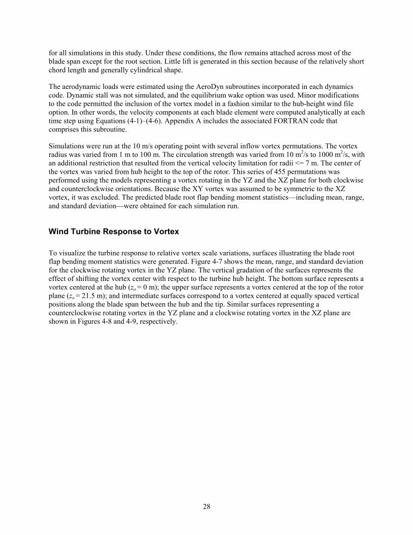
28

for all simulations in this study. Under these conditions, the flow remains attached across most of the blade span except for the root section. Little lift is generated in this section because of the relatively short chord length and generally cylindrical shape.

The aerodynamic loads were estimated using the AeroDyn subroutines incorporated in each dynamics code. Dynamic stall was not simulated, and the equilibrium wake option was used. Minor modifications to the code permitted the inclusion of the vortex model in a fashion similar to the hub-height wind file option. In other words, the velocity components at each blade element were computed analytically at each time step using Equations (4-1)–(4-6). Appendix A includes the associated FORTRAN code that comprises this subroutine.

Simulations were run at the 10 m/s operating point with several inflow vortex permutations. The vortex radius was varied from 1 m to 100 m. The circulation strength was varied from 10 m2/s to 1000 m2/s, with an additional restriction that resulted from the vertical velocity limitation for radii <= 7 m. The center of the vortex was varied from hub height to the top of the rotor. This series of 455 permutations was performed using the models representing a vortex rotating in the YZ and the XZ plane for both clockwise and counterclockwise orientations. Because the XY vortex was assumed to be symmetric to the XZ vortex, it was excluded. The predicted blade root flap bending moment statistics—including mean, range, and standard deviation—were obtained for each simulation run.

Wind Turbine Response to Vortex To visualize the turbine response to relative vortex scale variations, surfaces illustrating the blade root flap bending moment statistics were generated. Figure 4-7 shows the mean, range, and standard deviation for the clockwise rotating vortex in the YZ plane. The vertical gradation of the surfaces represents the effect of shifting the vortex center with respect to the turbine hub height. The bottom surface represents a vortex centered at the hub (zo = 0 m); the upper surface represents a vortex centered at the top of the rotor plane (zo = 21.5 m); and intermediate surfaces correspond to a vortex centered at equally spaced vertical positions along the blade span between the hub and the tip. Similar surfaces representing a counterclockwise rotating vortex in the YZ plane and a clockwise rotating vortex in the XZ plane are shown in Figures 4-8 and 4-9, respectively.

29

0 500 10000

50100

0

500

0

500

0

500

0

500

0

500

Gamma (m2/s)Radius (m)

Blad

e ro

ot f

lap

bend

ing

mom

ent m

ean (

kNm

)

0 500 10000

50100

0

100

0

100

0

100

0

100

0

100

200

Gamma (m2/s)Radius (m)

Blad

e ro

ot f

lap

bend

ing

mom

ent

rang

e (k

Nm

)

0 500 10000

50100

0

10

0

10

0

10

0

10

0

10

20

Gamma (m2/s)Radius (m)

Blad

e ro

ot f

lap

bend

ing

mom

ent

std.

dev

. (k

Nm

)

Figure 4-7. Blade load response to vortices of various size, circulation strength, and center

height above hub. The vortex rotates clockwise in the YZ plane with 10 m/s convection speed.

0 500 10000

50100

0

500

0

500

0

500

0

500

0

500

Gamma (m2/s)Radius (m)

Blad

e ro

ot f

lap

bend

ing

mom

ent m

ean

(kN

m)

0500

1000

050

100

0

100

0

100

0

100

0

100

0

100

200

Gamma (m2/s)Radius (m)

Blad

e ro

ot f

lap

bend

ing

mom

ent r

ange

(kN

m)

0 500 10000

50100

0

10

0

10

0

10

0

10

0

10

20

Gamma (m2/s)Radius (m)

Blad

e ro

ot f

lap

bend

ing

mom

ent s

td. d

ev. (

kNm

)

Figure 4-8. Blade load response to vortices of various size, circulation strength, and center

height above hub. The vortex rotates counterclockwise in the YZ plane with 10 m/s convection speed.

30

0 500 10000

50100

0

500

0

500

0

500

0

500

0

500

Gamma (m2/s)Radius (m)

Blad

e ro

ot f

lap

bend

ing

mom

ent m

ean (

kNm

)

0 500 10000

50 100

0

500

0

500

0

500

0

500

0

500

Gamma (m2/s)Radius (m)

Blad

e ro

ot f

lap

bend

ing

mom

ent

rang

e (k

Nm

)

0 500 10000

50100

0

25

0

25

0

25

0

25

0

25

50

Gamma (m2/s)Radius (m)

Blad

e ro

ot f

lap

bend

ing

mom

ent

std. d

ev. (k

Nm

)

Figure 4-9. Blade load response to vortices of various size, circulation strength, and center

height above hub. The vortex rotates clockwise in the XZ plane with convection speed of 10 m/s.

All surfaces show similarities in turbine response. The mean bending moment shows almost no variation with the scale and position of the vortex. The bending moment cyclic range and standard deviation, which contribute to fatigue damage, both increase as the radius of the vortex decreases and the circulation strength increases. Vortices with radii greater than 20 m to 30 m appear to contribute very little to load variation. This suggests that vortices on the scale of the rotor (turbine radius = 21.5 m) or smaller produce the load variation that leads to fatigue damage.

The clockwise rotating vortex in the YZ plane has the same rotational orientation as the wind turbine, so the rotational velocity of the vortex adds to the rotational velocity of the wind turbine. Intuitively, one would expect higher loads when the velocities add as compared to the case where the velocities subtract, the counterclockwise rotating vortex in the YZ plane. However, comparison of the bending moment range and standard deviation for both the clockwise and counterclockwise rotating vortex in the YZ plane (Figures 4-7 and 4-8) shows similar magnitudes for the vortex centered at the hub. The counterclockwise rotating vortex produces bending moment ranges that exceed those produced by the clockwise rotating vortex by approximately 20 kNm when the vortex is centered at the top of the rotor plane. In general, the loads produced when the vortex is centered at the hub are slightly higher than at any other location. Table 4-1 lists the magnitude of the bending moment ranges and standard deviations at the high magnitude edge for the surfaces that result from a vortex centered at the hub and a vortex centered at the top of the rotor.

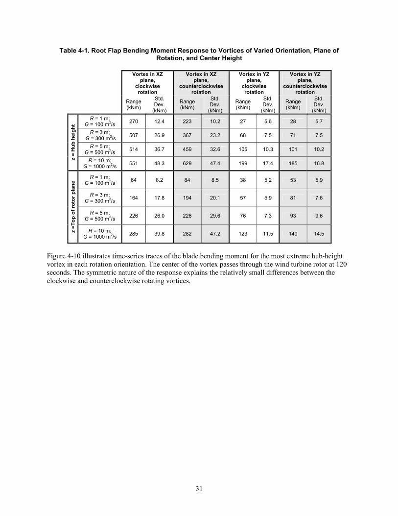
31

Table 4-1. Root Flap Bending Moment Response to Vortices of Varied Orientation, Plane of Rotation, and Center Height

Figure 4-10 illustrates time-series traces of the blade bending moment for the most extreme hub-height vortex in each rotation orientation. The center of the vortex passes through the wind turbine rotor at 120 seconds. The symmetric nature of the response explains the relatively small differences between the clockwise and counterclockwise rotating vortices.

Vortex in XZ plane,

clockwise rotation

Vortex in XZ plane,

counterclockwise rotation

Vortex in YZ plane,

clockwise rotation

Vortex in YZ plane,

counterclockwise rotation

Range (kNm)

Std. Dev.

(kNm)

Range (kNm)

Std. Dev.

(kNm)

Range (kNm)

Std. Dev.

(kNm)

Range (kNm)

Std. Dev.

(kNm) R = 1 m;

G = 100 m2/s 270 12.4 223 10.2 27 5.6 28 5.7

R = 3 m; G = 300 m2/s 507 26.9 367 23.2 68 7.5 71 7.5

R = 5 m; G = 500 m2/s 514 36.7 459 32.6 105 10.3 101 10.2

z =

Hub

hei

ght

R = 10 m; G = 1000 m2/s 551 48.3 629 47.4 199 17.4 185 16.8

R = 1 m; G = 100 m2/s 64 8.2 84 8.5 38 5.2 53 5.9

R = 3 m; G = 300 m2/s 164 17.8 194 20.1 57 5.9 81 7.6

R = 5 m; G = 500 m2/s 226 26.0 226 29.6 76 7.3 93 9.6

z =T

op o

f rot

or p

lane

R = 10 m; G = 1000 m2/s 285 39.8 282 47.2 123 11.5 140 14.5

32

110 112 114 116 118 120 122 124 126 128 1300

100

200

300

400

500

600

700

800

Time (s)

110 112 114 116 118 120 122 124 126 128 1300

100

200

300

400

500

600

700

800

Time (s)

Bla

de ro

ot fl

ap b

endi

ng m

omen

t (kN

m)

YZ Vortex, CWYZ Vortex, CCXZ Vortex, CWXZ Vortex, CC

YZ Vortex, CWYZ Vortex, CCXZ Vortex, CWXZ Vortex, CC

R = 10 m; G = 1000 m2/s; centered at hub height

R = 10 m; G = 1000 m2/s; centered at top of rotor

Bla

de ro

ot fl

ap b

endi

ng m

omen

t (kN

m)

Figure 4-10. Time-series traces of root flap bending moment resulting from vortex passage

This symmetry also exists for vortices in the XZ plane, as illustrated in Figure 4-10. For this reason, surfaces representing only a clockwise rotating vortex in the XZ plane are presented in Figure 4-9. Table 4-1, however, lists the magnitudes for both orientations at the edge of the surface with the highest magnitude for comparison. For vortices centered at hub height, the counterclockwise rotating vortex in the XZ plane has a steeper slope of blade bending moment range at the edge that corresponds to small radius and high circulation strength. On average, both clockwise and counterclockwise rotating vortices produce similar magnitude bending moment ranges for all vortex center locations. The vortex centered at the hub produces higher magnitude range loads than at any other vertical location. The bending moment range for a vortex centered at the top of the rotor plane produced about half the cyclic load as the vortex centered at the hub. However, the vortex centered at the top of the rotor could contribute to extreme peak loads. Although extreme load conditions are important design criteria, this issue is not addressed in this study. The vortex in the XZ plane produces cyclic range variations that exceed those produced by a vortex in the YZ plane by 2–10 times.

The highest magnitude bending moment range of 629 kNm, which results from a vortex of 10 m radius and 1000 m2/s circulation strength rotating counterclockwise in the XZ plane, compares favorably to the extreme range measured on the operating turbine in the 10 m/s wind speed bin (Figure 4-4). Again, complicating factors obscure this comparison. For instance, the operating turbine has a teetered hub, and the measured blade bending moment could include the result of teeter stop impact. Also, the blade bending moment responds with higher cyclic fluctuation when the blade pitch is adjusted to regulate power production. Finally, the mean wind speed during a 10-minute period can fluctuate significantly and the range statistic would not necessarily represent a single inflow event. The simulation does not include any pitch control or turbine dynamics so as to isolate the aerodynamic load induced by a vortex in the inflow. Regardless, the relative magnitude of bending moment ranges produced by the simulated vortices compares favorably to those observed in the experimental data.

33

A preliminary investigation of approximating the vortex flow field was performed using the AeroDyn code’s hub-height wind input file capability (Laino and Hansen 2001). The horizontal, or u, velocity component produced by a 10-m-radius, 500-m2/s circulation vortex at the top and bottom of the rotor was used to compute a time-varying, linear, vertical shear across the rotor. Similarly, the hub-height vertical, or w, velocity component was extracted from the vortex at each simulation time step. These values were used to create hub-height wind files that varied only the vertical shear, only the vertical wind component, and the combination of the two. AeroDyn assumes specified vertical wind velocity components to be uniform across the entire rotor. Figure 4-11 illustrates the time-varying bending moment response to the vortex, along with these three approximations. The amplitude of the bending moment produced by the vortex exceeds all three approximations. The vertical shear alone most closely maintains the cyclic response and amplitude magnitude of the three approximations. The vortex model, however, induces some cyclic bending moment variation at the peak amplitudes that is not captured by the approximations.

114 115 116 117 118 119 120 121 122 123 124200

250

300

350

400

450

500

550

600

Bla

de ro

ot fl

ap b

endi

ng m

omen

t (kN

m)

Time (s)

XZ Vortex, R = 10 m, G = 500 m 2/sVertical shear w component Vertical shear and w component

Figure 4-11. Comparison root flap bending moment response to vortex flow-field

approximations with actual vortex-induced bending moment

The aerodynamic response of a wind turbine to a vortex in the flow field should not be substantially different for two- or three-blade machines. This is demonstrated in Figure 4-12 where a dimensionless representation of the response surfaces for the bending moment coefficient range for the two-blade turbine is compared to that of a three-blade turbine where the vortex was centered both at the hub and at the top of the rotor. The three-blade turbine model is a 46-m, 750-kW rotor based on an initial iteration from the WindPACT rotor design study (Malcolm and Hansen 2002). It was modeled as a dynamically stiff turbine in the same manner as the two-blade turbine. The ratio of the vortex radius to the turbine radius is one dimensionless parameter. The vortex circulation was normalized with the following parameter:

∞= VRG To π2 (4-9)

The blade root bending moment was normalized with the following parameter:

3TPo RQB π= (4-10)

where

34

2

21

∞= VQP ρ

(4-11)

00.5

1

0

50

0.1

0.2

0.3

0.4

0

0.1

0.2

G/Go

T wo blades

R/RT

Ben

din

g m

omen

t co

effic

ien

t ran

ge

00 .5

1

0

50

0.1

0.2

0.3

0.4

0

0.1

0.2

G/Go

Three blades

R/RT

Bend

ing

mom

ent

coef

ficie

nt r

ange

Figure 4-12. Dimensionless bending moment response to vortex parameter variation for

two- and three-blade turbines

Figure 4-12 shows that the bending moment ranges for the two- and three-blade turbines are similar whether the vortex is centered at the hub or at the top of the rotor. The three-blade turbine has a slightly steeper slope as the normalized radius is decreased and the normalized circulation is increased. However, the similarity in the aerodynamic response of the two turbines is confirmed.

Chapter Conclusions This analytic study identifies the aerodynamic response of a dynamically stiff wind turbine to analytic vortex structures in the inflow. The vortex variation included radius, circulation strength, location with respect to the hub, orientation, and plane of rotation. Blade response under each permutation was obtained through simulation using both the FAST and SymDyn wind turbine dynamics codes, although only FAST results were presented here. The blade responses were presented in surface plots that illustrate the variations in blade load as a result of vortex passage through the rotor. Because of symmetry, the turbine response to clockwise and counterclockwise rotating vortices was similar for vortices in the YZ and XZ planes. This is also assumed to be true for vortices in the XY plane. A counterclockwise rotating vortex in the XZ plane and aligned with the hub produced the greatest load variation. Decreased load variation was observed as the vortex was moved vertically to the top of the rotor plane, but these loads still exceeded those observed as a result of passage of a vortex in the YZ plane. Vortices in the XY plane were assumed to be symmetric to those in the XZ plane. A vortex in the XZ plane is most representative of the type of vortical structure that could occur as a result of a Kelvin-Helmholtz instability in the atmospheric boundary layer in which the turbine operates. The mean bending moment is largely unaffected under any of these parameter variations. Vortices of radii smaller than 20 m to 30 m, on the scale of the rotor or

35

smaller, produce bending moment fluctuations that contribute to fatigue damage. Similar bending moment response is produced by a dynamically stiff three-blade turbine, as would be expected. Vertical shear across the rotor approximates the vortex-induced bending moment cyclic variation more closely than the hub-height vertical wind component or a combination of vertical shear and vertical velocity. However, the amplitude of the vortex-induced bending moment is underestimated, and some higher frequency dynamics are not captured.

36

Chapter 5

Load Mitigation through Advanced Control To determine whether advanced control can be applied successfully to the wind turbine/vortex interaction problem, specific restrictions were identified. The control studies were performed on a three-blade, variable-speed wind turbine. This restricts the study to the vortex/wind turbine interaction because any commercial two-blade wind turbine would have a teetered rotor, which complicates the dynamic response. The control study was also restricted to Region 3 operation—the simplest regime in which to design control algorithms. This operating regime occurs at wind speeds above rated, where the primary control objective is to regulate rotor speed. The vortex characteristics that contribute to the highest blade cyclic loads identified in Chapter 4 were used to restrict the control study. A vortex rotating in the XZ plane and centered on the hub produces the most significant bending moment range. Because little difference in response resulted from the orientation of the vortex, the control study was restricted to a counterclockwise vortex orientation.

A vortex representing a point near the center of the sloped surface in Figure 4-12 was selected for the control design. This three-blade wind turbine would be in Region 3 operation when the mean wind speed is 18 m/s. The vortex parameters were scaled using the dimensionless quantities in Equations (4-9)–(4-11). The resulting vortex had a radius of 10.7 m, circulation strength of –577 m2/s, and convection speed of 18 m/s. Simulations represented a time period of 55 seconds with the vortex center passing through the rotor at 45 seconds (at t = 0, (x0, y0, z0) = (-810,0,0)). The first 20 seconds of simulation were neglected to exclude start-up transients in the simulation.

The SymDyn code was used exclusively for the control design studies because linearization routines and control design tools were available; at the time of this study the FAST code did not have comparable tools.

Baseline PI Controller A baseline controller designed using commonly accepted tools was required for comparison to advanced control designs. The industry standard wind turbine controller uses PID algorithms. Figure 5-1 illustrates the control regions as relationships between generator torque and rotor speed. In Region 2, the rotor speed is permitted to vary by maintaining a constant tip speed ratio. This is accomplished by controlling the generator torque according to Equation (5-1). The peak power coefficient and corresponding tip speed ratio were determined using a wind turbine performance code, WT_Perf, that maps the power coefficient over a range of tip speed ratios and blade pitch angles (Buhl 2000).

23

5

2Ω

=

MAX

PMAXTE

CRQλ

ρπ

(5-1)

37

0

50

100

150

200

250

300

0 5 10 15 20 25 30 35

Rotor speed (rpm)

Gen

erat

or to

rque

(kN

m)

Region 2

Region 3

Figure 5-1. Generator torque versus rotor speed curve for generator torque controller

In Region 3, the control objective is to maintain constant power by regulating rotor speed. The generator torque is held constant. The rotor speed is permitted to deviate from the rated speed by a small percentage. For the three-blade turbine, a range of ±3% was selected. The transition between the two regions is generally accomplished by representing an induction generator with 5% slip. The linear part of the curve connects the low end of the Region 3 speed (–3% of rated) to the Region 2 curve.

The baseline controller for Region 3 is a PI controller based on a design for NREL’s Controls Advanced Research Turbine (CART), a variable-speed version of the ART. A series of step changes in wind speed was input to the three-blade turbine simulation, and the rotor speed and pitch actuation recorded. Beginning with the gains for the CART, adjustments were made to these gains to achieve similar performance between the two simulation models. Table 5-1 compares the performance metrics. The root mean square (RMS) of the speed error indicates the deviation from the desired rotor speed. When expressed as percentage of rated, the desired magnitude is restricted to 3% for the three-blade turbine and 1% for the two-blade turbine. These gains maintain speed regulation of the three-blade turbine similarly to the two-blade turbine. The RMS of pitch acceleration indicates actuator demand levels, which are also similar for the two turbine models. The gains associated with the values for the three-blade turbine in Table 5-1 are P = 60 and I = 30.

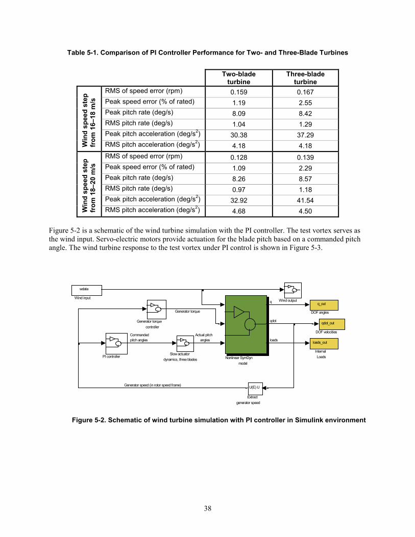
38

Table 5-1. Comparison of PI Controller Performance for Two- and Three-Blade Turbines

Two-blade

turbine Three-blade

turbine RMS of speed error (rpm) 0.159 0.167 Peak speed error (% of rated) 1.19 2.55 Peak pitch rate (deg/s) 8.09 8.42 RMS pitch rate (deg/s) 1.04 1.29 Peak pitch acceleration (deg/s2) 30.38 37.29

Win

d sp

eed

step

fr

om 1

6–18

m/s

RMS pitch acceleration (deg/s2) 4.18 4.18 RMS of speed error (rpm) 0.128 0.139 Peak speed error (% of rated) 1.09 2.29 Peak pitch rate (deg/s) 8.26 8.57 RMS pitch rate (deg/s) 0.97 1.18 Peak pitch acceleration (deg/s2) 32.92 41.54

Win

d sp

eed

step

fr

om 1

8–20

m/s

RMS pitch acceleration (deg/s2) 4.68 4.50 Figure 5-2 is a schematic of the wind turbine simulation with the PI controller. The test vortex serves as the wind input. Servo-electric motors provide actuation for the blade pitch based on a commanded pitch angle. The wind turbine response to the test vortex under PI control is shown in Figure 5-3.

Wind output wdata

Wind input

Slow actuatordynamics, three blades

PI controller Nonlinear SymDynmodel

loads_out Internal Loads

Generator torque controller

UU(E)

Extractgenerator speed

qdot_out

DOF velocities

q_out DOF angles

q

qdot

Generator speed (in rotor speed frame)

loadsCommanded pitch angles Actual pitch

angles

Generator torque

Figure 5-2. Schematic of wind turbine simulation with PI controller in Simulink environment

39

20 25 30 35 40 45 50 55-1

-0.5

0

0.5

1

1.5

2

Time (s)

Blad

e fla

p an

gle

(deg

)

Blade 1Blade 2Blade 3

20 25 30 35 40 45 50 5512

14

16

18

20

22

24

Time (s)

Bla

de p

itch

angl

e (d

eg)

20 25 30 35 40 45 50 5526.2

26.4

26.6

26.8

27.0

27.2

Time (s)

Roto

r sp

eed

(rpm

)

Figure 5-3. Wind turbine response to test vortex with PI controller

40

The blade flap angles indicate significant motion associated with vortex passage. The wind force that results in blade root flap bending moment also causes blade flap angle deflection. Note that the PI controller commands collective pitch angles. This means that each blade is pitched the same amount and in the same direction as the vortex passes. Figure 5-3 presents the baseline response to which all DAC designs are compared.

DAC Design Methodology Linearized Wind Turbine Model The first requirement for design of a DAC algorithm is a linear model of the plant, or in this case, the wind turbine. The equations of motion of the nonlinear wind turbine implemented in SymDyn are presented below, where q is the vector of degrees of freedom.

0)),,,(,,,()( =+ φWqqLQqqfqqM E (5-2)

A linear representation of these equations is needed for control design, specifically for designing a state estimator. This is accomplished by perturbing each variable about an operating point. In this study, the operating point was specified to be a uniform wind of 18 m/s; the u velocity component is 18 m/s, and the w velocity component is 0 m/s. The perturbation equations are of the following form:

qqq OP ∆+= ; qqq OP ∆+= ; qqq OP ∆+= ; WWW OP ∆+= ; φφφ ∆+= OP (5-3)

Substituting Equation (5-3) into Equation (5-2) and expanding in a Taylor series yields the linear wind turbine equations of motion:

φ∆+∆=∆+∆+∆ )()()()()( tHWtEqtKqtGqtM (5-4)

Equation (5-4) is transformed into a first-order state-space form for control design.

DD utButBxtAx )()()( ++= (5-5)

where

−−

= −− )()()()(0

)( 11 tGtMtKtMI

tA DOFDOFDOFDOF xNNxNN , the state matrix,

= − )()(

0)( 1 tHtM

tB BDOF xNN , the control input matrix,

= − )()(

0)( 1 tEtM

tB DDOF xNND , the wind input matrix,

Tqqtx ][)( ∆∆= , the state vector of perturbed coordinates,

41

φ∆=u , the control input (vector of blade pitch angles), and WuD ∆= , the wind disturbance input.

The linear parameters (A, B, BD) are periodic, with the period equal to the time required for one rotor revolution. These parameters are computed for several azimuth angle positions and then averaged over the equivalent of one rotor revolution. This method was successfully developed by Stol (2001). All subsequent notations of the linear system parameters assume that they are time-invariant.

For this study, the linear plant model outputs are state measurements such as the rotor speed and the blade flap angle. This linear model is implemented in the Simulink environment for the purpose of state-space-based control design; now x , u , and Du are functions of time. The state vector is defined as follows:

=

3

2

1

1

3

2

1

1

βββψβββψ

x

(5-6)

The linear model includes four degrees of freedom: rotor rotation, and blade flap for each of three blades. Because the drive-train torsion degree of freedom is not modeled, the generator speed is proportional to the rotor speed by the gear ratio of the gearbox. Thus, rotor speed and generator speed are used interchangeably in this text. The linear plant model is presented in Equations (5-7) and (5-8) where control inputs, u , are dimension M (three pitchable blades); plant outputs, y , are dimension P (1 or 4 for either generator speed alone or generator speed and 3 blade flap angles); and states, x , are dimension N (8).

)()()()( tuBtuBtxAtx DD++= (5-7)

)()( txCty = ; 0)0( xx = (5-8)

The number of disturbance inputs, Du , varies from 1 to 60 depending on the disturbance generator model chosen. Figure 5-4 shows a schematic of a general DAC design built around a linear plant model.

Rotor azimuth position Blade 1 flap angle Blade 2 flap angle Blade 3 flap angle Rotor speed Blade 1 flap rate Blade 2 flap rate Blade 3 flap rate

42

o

DD

xxCxy

uBBuAxx

==

++=

)0(

0)0(ˆ)ˆ(ˆˆ

ˆˆ

=−+=

Θ=

D

DDD

DD

zyyKzFz

zu

0)0(

ˆ

DD

DD

DD

zz

zFzzu

=

=Θ=

yy ˆ−

Du

x

Dz

yDu

u

DG

Θ

0)0(ˆˆˆ

)ˆ(ˆˆˆ

==

−+++=

xxCy

yyKuBBuxAx

X

DD

XG

+

Plant State Estimator

Plant

Disturbance Generator

Disturbance Estimator

Figure 5-4. Schematic of general DAC design

Disturbance Waveform Generator The wind is modeled as a persistent disturbance of known waveform but unknown amplitude, as presented by Johnson (1976). The disturbance inputs, Du , have dimension MD, and the disturbance states,

Dz , have dimension ND.

)()( tztu DD Θ= (5-9)

)()( tzFtz DD = ; 0)0( DD zz = (5-10)

The matrices F and Θ are selected to represent the waveform approximation of the disturbance that enters the linear system. The initial condition, 0

Dz , is not known. For instance, a step disturbance, which has been shown to be an adequate approximation of uniform wind speed for wind turbine controllers (Kendall 1997; Stol, Rigney, and Balas 2000; Stol and Balas 2002; Wright 2003), is modeled with F = 0 and Θ = 1. A sinusoid of unknown amplitude and frequency of Ωt would be modeled as follows:

Ω−

=010

2F ; [ ]01=Θ (5-11)

43

Composite (Plant/Disturbance) State Estimator Because the wind disturbance inputs cannot be directly measured, the disturbance states are estimated from the plant outputs by augmenting the usual plant state estimator. The linear plant state estimator is of the form:

))(ˆ)(()(ˆ)()(ˆ)(ˆ tytyKtuBtuBtxAtx XDD −+++= (5-12)

)(ˆ)(ˆ txCty = ; 0)0(ˆ =x (5-13)

The state estimator is appended with the following disturbance estimator that uses feedback correction from the plant output error.

)(ˆ)(ˆ tztu DD Θ= (5-14)

))(ˆ)((ˆ)(ˆ tytyKzFtz DDD −+= ; 0)0(ˆ =Dz (5-15)

The estimator error is defined as the difference between the state and the state estimate as follows:

−−

=

=

)(ˆ)()(ˆ)(

)()(

)(tztz

txtxtete

teDDD

X (5-16)

The estimator error equation is:

)()()( teCKAte −= (5-17)

where

Θ=

FBA

A D

0; [ ]0CC = ; and

=

D

X

KK

K . (5-18)

Thus, when ( )CA, is observable, the gains, KX and KD, can be chosen through arbitrary pole placement to ensure exponential decay of the error between the states and the state estimates as well as the error between the disturbance and the disturbance estimate.

Control Law for DAC The ideal control law, assuming complete knowledge of the states and the disturbance inputs, would be as follows:

)()()(* tzGtxGtu DDX += (5-19)

The closed loop system would be obtained by substituting Equation (5-19) into Equation (5-7) to obtain Equation (5-20).

44

)()()()()( tzBBGtxBGAtx DDDX Θ+++= (5-20)

When (A,B) is controllable, arbitrary pole placement may be used to determine GX such that the system control has appropriate transient behavior. The selection of the disturbance state gain, GD, permits cancellation, or mitigation, of the disturbance effect on the system.

0→Θ+ DD BBG (5-21)

The Moore-Penrose pseudoinverse of B (B+) is used to solve for GD.

Θ−=Θ−= −+D

TTDD BBBBBBG ))(( 1 (5-22)

The ideal control law is not realizable because the states and disturbance inputs could never be known exactly. The estimates are substituted in the control law along with the error between the states and estimates.

)()()(ˆ)(ˆ)( * teGtutzGtxGtu DDX −=+= (5-23) where

[ ]DX GGG = . (5-24)

The error dissipates exponentially because of the selection of KX and KD in Equation (5-17).

In summary, the linear plant model is used to create a plant state estimator. A disturbance generator model, defining F and Θ, is developed to simulate the waveform of the wind input to the wind turbine. This disturbance generator is used to create a disturbance state estimator, which is appended to the plant state estimator. If ( )CA, is observable, the gains, KX and KD, are selected to dissipate the error between the state and the state estimate. If (A,B) is controllable, the gain, GX, is selected to provide desired transient behavior of the plant states. The realizable control law results in desirable transient stability of the closed loop system. The disturbance gain, GD, is selected to minimize the effect that the disturbance introduces to the system. In this way the disturbance is “accommodated” through the control design.

Performance Assessment Criteria The selection of the state and estimator gains is done using a linear quadratic regulator (LQR) as implemented in MATLAB© (The Mathworks, Inc. 2002). This formulation seeks a solution to the algebraic Riccati equation (Kwakernaak and Sivan 1972) to minimize a cost function

∫∞

+=0

)( dtuRuxQxJ TT (5-25)

where Q is the symmetric, positive semi-definite weighting on the states, and R is the symmetric, positive definite weighting on the inputs, u = Gx. The cost function, J, has no physical significance, but it permits

45

a solution that balances state regulation with input amplitude. For instance, a wind turbine control system balances rotor speed regulation with pitch actuator demand. Using an LQR to design state feedback and estimator feedback gains is especially useful when multiple states are modeled.

The servo-electric motors that pitch the blades convert the commanded pitch angle to a velocity command. Figure 5-5 presents a schematic of the pitch actuator system. The proportional gain, 5 deg/s per degree of error, converts the commanded pitch angle to velocity. In the PI controller, this low-valued gain introduces a lag in pitch actuation to reduce actuator demand. For the state-space-based control designs that seek to meet objectives in addition to rotor speed regulation, this gain was increased to 100 deg/s per degree of error. This permits the controller to more closely follow the commanded pitch angle. The servo-electric motors are rate-limited to 18 deg/s. The acceleration is limited to around 150 deg/s2. Actuator demand for the wind turbine control designs should not exceed these values.

Pitch rate

Pitch acceleration

1 Actual

pitch angles

phidotdot_out

phidot_out

1s

1s

1s

1s

1s

1s

605

60

60

5

5 Demux 1

Commanded pitch angles

Blade #2

Blade #1

Blade #3

Figure 5-5. Schematic of blade pitch actuators (with slow proportional gain) in Simulink

environment

In Region 3 operation, the wind turbine rotor speed should not exceed 3% of the rated rotor speed, or 27.4 rpm for the three-blade turbine. This limit is prescribed by the generator specifications. In addition to limiting the peak rotor speed, minimizing fluctuation about the rated speed during turbine operation is generally desirable. The RMS of the error between the actual and desired rotor speeds is a useful measure of the speed regulation.

Blade root flap bending moments are the most commonly used measures of blade loads associated with the force imparted by the wind (blade root edge bending moments are governed by the inertial and gravitational load fluctuations). The damage equivalent fatigue load, Fe, defined earlier, was used to compare wind turbine simulation response using different control algorithms. Because the damage equivalent load is dominated by the largest cyclic amplitude, the range of flap bending moment over the simulation is also examined. Some of the problems inherent in the measured data that were described in Chapter 3 were not at issue in the simulations. There is one event in each simulation run that occurs at 45 seconds, passage of the test vortex. The convection speed did not fluctuate during the simulation, so

46

the bending moment range is associated with the passage of the vortex. Because the inflow can be exactly duplicated from one simulation to another, comparisons are easily made using these blade bending moment metrics.

Note that controller inputs, considered to be measurements made on the wind turbine, do not include blade bending moments. In some control designs, the blade flap angles are considered to be measurements. The flap angle represents the blade flap deflection caused by the wind force that contributes to the root bending moment. In this way, the flap angle and bending moments are related.

In summary, the metrics used to evaluate control designs included actuator demand, speed regulation, and load mitigation. The blade pitch actuator peak rate and peak acceleration were limited to 18 deg/s and 150 deg/s2, respectively. The RMS of rotor speed error was minimized, and the peak rotor speed was restricted to 3% of the rated speed. The blade root flap bending moment range and damage equivalent fatigue load were minimized. Tables 5-4–5-10 compare the performance of controllers and include the maximum equivalent fatigue load of the three blades and the bending moment range for each blade.

DAC Designs Ten-Blade Element Disturbance Model The wind turbine simulation codes use blade-element-momentum theory (Eggleston and Stoddard 1987) to compute the aerodynamic loads that the wind imparts to the blade. This assumes that each blade can be subdivided into elements along the span. The aerodynamic load is computed for each element using the velocity components computed at the blade element. To capture the details of the vortex as a disturbance model for control design, 10-blade elements along the span of each blade were used. The disturbance model assumed a u and w velocity component step change at each of these 10 elements for each of the three blades for a disturbance model consisting of 60 inputs. For the step change disturbance, F = 0 and Θ = 1. For the 60 inputs, these matrices are 60 rows by 60 columns, where F is populated with zeros and Θ is the identity matrix of dimension 60.

To create the wind input matrix, BD, each of the 60 disturbance inputs was perturbed independently. The operating point was defined to be a uniform wind of 18 m/s. In other words, the u velocity component was perturbed to 18.1 m/s and to 17.9 m/s at each blade element for each blade. The w velocity component was perturbed to 0.1 m/s and to –0.1 m/s at each blade element for each blade. The average of the two perturbations results in the value inserted in the BD matrix, which is presented in Appendix C. The values that represent velocity perturbations for inboard elements are of very low magnitude; those that represent velocity perturbations for the outboard elements are of higher magnitude. This is expected because velocity changes on the outboard sections contribute more strongly to blade flap angle deflection. The GD matrix (included in Appendix C) was obtained using the Moore-Penrose pseudoinverse.

The state gain, GX, was determined using LQR. Initially, step changes in wind speed were input to the simulation and the weightings on the diagonal entries in Q associated with the rotor states were adjusted until the speed regulation and pitch actuation were similar to that of the PI controller. Next, the blade state gains were adjusted by adding weight in the Q matrix to reduce the blade cyclic loading and fatigue equivalent load resulting from the step change wind input. Table 5-2 presents the speed regulation and actuator demand for the baseline PI controller and this state-space controller.

47

Table 5-3 compares the open loop and closed loop poles. The last six entries are associated with the blade states. The addition of damping through feedback reduces the flap deflection. Appendix C contains the GX, Q, and R matrices for the completed design.

Table 5-2. Comparison of PI Controller and State-Space Controller Performance for Step Wind Input

PI controller State-space

controller RMS of speed error (rpm) 0.167 0.14 Peak speed error (% of rated) 2.55 2.41 Peak pitch rate (deg/s) 8.42 14.80 RMS pitch rate (deg/s) 1.29 0.84 Peak pitch acceleration (deg/s2) 37.29 399.87

Win

d sp

eed

step

fr

om 1

6–18

m/s

RMS pitch acceleration (deg/s2) 4.18 14.81 RMS of speed error (rpm) 0.139 0.12 Peak speed error (% of rated) 2.29 2.03 Peak pitch rate (deg/s) 8.57 14.60 RMS pitch rate (deg/s) 1.18 0.77 Peak pitch acceleration (deg/s2) 41.54 398.95

Win

d sp

eed

step

fr

om 1

8–20

m/s

RMS pitch acceleration (deg/s2) 4.50 14.52

Table 5-3. Poles for Open Loop System and Closed Loop System

Open Loop Poles Closed Loop Poles 0 – 1.02 + 0.21i – 0.21 – 1.02 – 0.21i – 3.58 + 19.03i – 7.03 + 1.33i – 3.58 – 19.03i – 7.03 – 1.33i – 3.66 + 18.84i – 7.11 + 1.08i -- 3.66 – 18.84i – 7.11 – 1.08i – 3.66+ 18.84i – 7.11 + 1.08i – 3.66 – 18.84i – 7.11 – 1.08i

The next step is to design a state estimator for the system by augmenting the turbine states with the disturbance states. The observability condition on ( )CA, is not met with this 60-input disturbance model. However, creation of an FSFB controller using this disturbance model yields the best-case scenario. This assumes that each state in the turbine model and in the disturbance model is a known quantity. Using the test vortex as wind input, the u and w time-varying velocity components associated with each blade element were output from the rigid model simulation as a text file. This text file was then read into the controller simulation to result in known disturbance input. Figure 5-6 is a diagram of this FSFB control system.

48

Wind output

Subtract operating point

K*u State

feedback gain

phi_op Operating

pitch angle

Nonlinear SymDynmodel

loads_out Internal loads

Qe

Generator torque

Fast actuatordynamics, three blades

K*u Disturbance feedback gain qdot_out

DOF velocities

q_out DOF angles

elem_data Blade element

velocity components

qdot

qdot

q

q

States, x

loads

Figure 5-6. Schematic of FSFB controller using 10-element disturbance model in Simulink

environment

Table 5-4 compares the simulated turbine response to the test vortex using FSFB of the 10-element disturbance model and the response using the PI controller. A reduction in blade fatigue equivalent load as high as 30% seems possible if the disturbance model incorporates enough detail of the vortex in the inflow. Reduction of each blade’s cyclic amplitude of more than 30% is also achievable. Note that the FSFB controller exceeds the pitch actuator rate and acceleration limits. FSFB causes the pitch input to constantly adjust because new disturbance information is presented. There is no settling time as there is when the input is limited or nonexistent.

Table 5-4. Comparison of PI Controller and FSFB of 10-Element Disturbance Model Controller Performance for Test Vortex (RFB = root flap bending moment)

Test VortexPI FSFB Difference

RMS speed error (rpm) 0.05 0.05 -6%Max speed error (% rated) 1.6 1.4 -17%Max pitch rate (deg/s) 9.9 31.5 219%RMS pitch rate (deg/s) 1.03 2.81 174%Max pitch acceleration (deg/s^2) 67.7 807.2 1092%RMS pitch acceleration (deg/s^2) 8.02 40.63 407%Flap damage equivalent load (kNm) 369 258 -30%Blade 1 RFB range (kNm) 422 288 -32%Blade 2 RFB range (kNm) 551 386 -30%Blade 3 RFB range (kNm) 381 249 -35%

Figure 5-7 shows the wind turbine time-series response to the test vortex. The flap angle deflection is reduced compared to that corresponding to the PI controller in Figure 5-3. This contributes to blade flap damage equivalent load reduction. Also, the blade pitch angles are commanded independently in response to the velocity conditions associated with the vortex at each blade position. Because others have successfully implemented an observable disturbance model consisting of a step change in hub-height wind speed for other control objectives (Kendall 1997; Stol, Rigney, and Balas. 2000; Stol and Balas 2002; Wright 2003), this was attempted next.

49

20 25 30 35 40 45 50 55-1

-0.5

0

0.5

1

1.5

2

Time (s)

Blad

e fla

p an

gle

(deg

)Blade 1Blade 2Blade 3

20 25 30 35 40 45 50 5512

14

16

18

20

22

24

Time (s)

Bla

de p

itch

angl

e (d

eg)

20 25 30 35 40 45 50 5526.2

26.4

26.6

26.8

27.0

27.2

Time (s)

Roto

r sp

eed

(rpm

)

Figure 5-7. Wind turbine response to test vortex with FSFB of 10-element disturbance model controller

50

DAC with Hub-Height Wind Speed Disturbance Model (DAC HH) The simplest disturbance model used for wind turbine control design consists of a step change in uniform wind speed. In this case, F = 0, Θ = 1, and uD = zD. The matrix, BD, is determined by perturbing the hub-height wind speed about 18 m/s. The matrix GD is obtained using the Moore-Penrose pseudoinverse. The matrix GX is obtained using LQR with the Q matrix weightings that result from the FSFB controller design. The state estimator is constructed because observability of ( )CA, is achieved when the single disturbance state is appended to the plant states. The estimator gains, KX and KD, are determined using LQR. Only the rotor speed is assumed to be a measured output of the plant. All gain and weighting matrices are included in Appendix C. Figure 5-8 is a schematic of the simulation, and the response to the test vortex for this controller is compared to that of the PI controller in Table 5-5.

Generator torque

x

W ind output wdata W ind input

K*u

Turbine measurements Subtract operating point

phi_op Operating

pitch angle

Nonlinear SymDynmodel

loads_out Internal loads

Fast actuatordynamics, three blades

qdot_out DOF velocities

q_out DOF angles

DAC controller

CART torque controller

qdot

qdot

q

q

States, x

wdata

u loads

y

Figure 5-8. Schematic of wind turbine simulation with DAC controller in Simulink

environment

51

Table 5-5. Comparison of PI Controller and DAC HH Controller Performance for Test Vortex, Full-Field Turbulence, and Vortex Superimposed on Turbulence

Test Vortex Full-Field Turbulence Turbulence + vortex

PI DAC HH Difference PI DAC HH Difference PI DAC HH DifferenceRMS speed error (rpm) 0.05 0.05 -4% 0.32 0.30 -7% 0.33 0.31 -7%Max speed error (% rated) 1.6 1.6 -5% 2.4 2.6 5% 2.4 2.5 3%Max pitch rate (deg/s) 9.9 13.3 35% 7.4 9.0 21% 9.8 12.0 23%RMS pitch rate (deg/s) 1.03 1.42 38% 2.73 2.85 4% 2.93 3.13 7%Max pitch acceleration (deg/s^2) 67.7 112.7 67% 33.4 56.6 69% 49.5 74.5 50%RMS pitch acceleration (deg/s^2) 8.02 12.17 52% 10.76 15.92 48% 12.31 18.27 48%Flap damage equivalent load (kNm) 369 356 -4% 268 272 1% 372 382 3%Blade 1 RFB range (kNm) 422 410 -3% 317 304 -4% 510 518 1%Blade 2 RFB range (kNm) 551 531 -4% 310 312 1% 555 570 3%Blade 3 RFB range (kNm) 381 398 4% 396 401 1% 521 527 1%

A full-field turbulence wind file with a mean wind speed of 18 m/s was created using SNWind (Kelley 1992, Buhl 2003). The center block of Table 5-5 compares the DAC controller (DAC HH) and the PI controller response to the turbulent wind. The last block compares the performance of the two controllers to the test vortex superimposed on the turbulent wind (vortex centered at 45 seconds). Appendix A contains the SNWind input file used to generate a full-field turbulence file and describes the method used to superimpose the vortex on the turbulence. The DAC HH controller achieves slight load mitigation for the vortex alone, but this is lost when turbulence is added. This DAC design approach performs very similarly to the PI controller, a conclusion further evidenced in Figure 5-9, which shows the time-series response. The blade flap angles and commanded pitch angles are similar to those shown in Figure 5-3. This DAC design commands collective blade pitch, which does not accommodate the vortex passage. Obviously the disturbance must incorporate some element of the vortex dynamics to predict the different blade loads that result from vortex passage.

52

20 25 30 35 40 45 50 55-1

-0.5

0

0.5

1

1.5

2

Time (s)

Blad

e fla

p an

gle

(deg

)

Blade 1Blade 2Blade 3

20 25 30 35 40 45 50 5512

14

16

18

20

22

24

Time (s)

Bla

de p

itch

angl

e (d

eg)

20 25 30 35 40 45 50 5526.2

26.4

26.6

26.8

27.0

27.2

Time (s)

Roto

r sp

eed

(rpm

)

Figure 5-9. Wind turbine response to test vortex with DAC HH controller

53

DAC with One-Blade Element Disturbance Model (DAC 1 BE) A disturbance model based on the 10-element model, but modified to include only the velocities associated with each blade tip (one blade element), was constructed because it is observable. The disturbance consisted of six inputs representing the u and w velocity components at the tip element of each blade. The tip element was chosen because it is most strongly related to the blade flap deflection. Each input was modeled as a step change in wind speed. The F and Θ matrices are identical to those in the 10-element model except that they are of dimension 6. The wind input matrix, BD, included in Appendix C, was obtained by perturbing each velocity component on each blade independently. The disturbance gain matrix, GD, was obtained using the Moore-Penrose pseudoinverse. The state gain matrix, GX, was determined using LQR, and the weighting matrices are included with GX in Appendix C. Only the rotor position and speed states were weighted because the disturbance model associated with each blade contributes to the flap angle deflection. Accommodating the disturbance should correspond to decreased flap angle deviation, which, in turn, reduces the blade loads. Rotor speed and each blade flap angle were assumed to be measurements input to the controller. Because the reduced disturbance model with these plant measurements met the observability condition for ( )CA, an estimator was designed. Again, LQR was used to determine the state estimator gain, KX, and the disturbance estimator gain, KD. The gains and weighting matrices are in Appendix C.

A simulation using the test vortex as the wind input was performed with this DAC design (DAC 1 BE). The response is compared to that of the PI controller in Table 5-6. The full-field turbulence data and the vortex superimposed on the turbulence were also introduced as wind input for this controller. Although some mitigation in equivalent fatigue load is achieved with the DAC design, the speed regulation for the cases with turbulence is unacceptable because the 3% rated speed limit is exceeded. The time-series output for the vortex alone is shown in Figure 5-10. It shows that the pitch controller commands collective blade pitch that is incapable of accommodating the vortex disturbance.

Table 5-6. Comparison of PI Controller and DAC 1 BE Controller Performance for Test Vortex, Full-Field Turbulence, and Vortex Superimposed on Turbulence

Test Vortex Full-Field Turbulence Turbulence + Vortex

PID DAC 1 BE Difference PID DAC 1 BE Difference PID DAC 1 BE DifferenceRMS speed error (rpm) 0.05 0.09 73% 0.32 0.81 152% 0.33 0.81 144%Max speed error (% rated) 1.6 1.8 7% 2.4 7.4 205% 2.4 7.4 204%Max pitch rate (deg/s) 9.9 2.3 -77% 7.4 3.5 -53% 9.8 3.6 -63%RMS pitch rate (deg/s) 1.03 0.26 -75% 2.73 1.60 -41% 2.93 1.66 -43%Max pitch acceleration (deg/s^2) 67.7 14.1 -79% 33.4 9.0 -73% 49.5 11.3 -77%RMS pitch acceleration (deg/s^2) 8.02 1.52 -81% 10.76 2.71 -75% 12.31 3.05 -75%Flap damage equivalent load (kNm) 369 329 -11% 268 252 -6% 372 354 -5%Blade 1 RFB range (kNm) 422 404 -4% 317 277 -13% 510 496 -3%Blade 2 RFB range (kNm) 551 492 -11% 310 351 13% 555 528 -5%Blade 3 RFB range (kNm) 381 331 -13% 396 368 -7% 521 524 1%

54

20 25 30 35 40 45 50 55-1

-0.5

0

0.5

1

1.5

2

Time (s)

Blad

e fla

p an

gle

(deg

)

Blade 1Blade 2Blade 3

20 25 30 35 40 45 50 5512

14

16

18

20

22

24

Time (s)

Bla

de p

itch

angl

e (d

eg)

20 25 30 35 40 45 50 5526.2

26.4

26.6

26.8

27.0

27.2

Time (s)

Roto

r sp

eed

(rpm

)

Figure 5-10. Wind turbine response to test vortex with DAC 1 BE controller

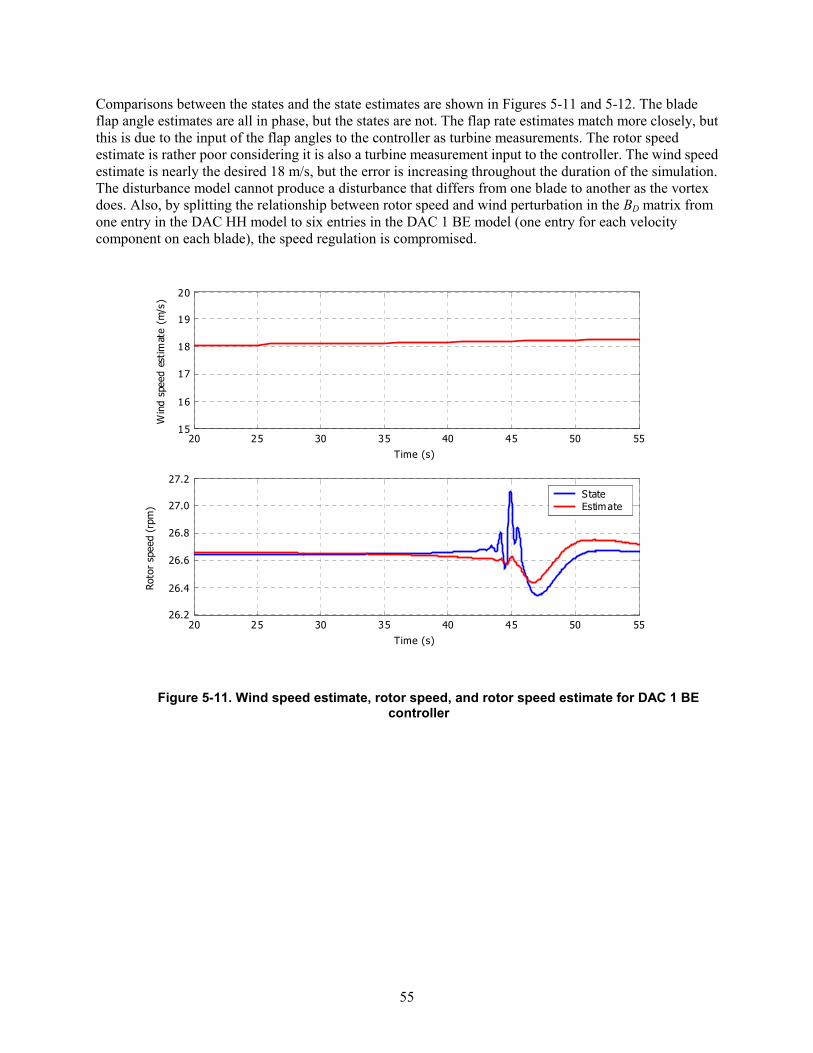
55

Comparisons between the states and the state estimates are shown in Figures 5-11 and 5-12. The blade flap angle estimates are all in phase, but the states are not. The flap rate estimates match more closely, but this is due to the input of the flap angles to the controller as turbine measurements. The rotor speed estimate is rather poor considering it is also a turbine measurement input to the controller. The wind speed estimate is nearly the desired 18 m/s, but the error is increasing throughout the duration of the simulation. The disturbance model cannot produce a disturbance that differs from one blade to another as the vortex does. Also, by splitting the relationship between rotor speed and wind perturbation in the BD matrix from one entry in the DAC HH model to six entries in the DAC 1 BE model (one entry for each velocity component on each blade), the speed regulation is compromised.

20 25 30 35 40 45 50 5526.2

26.4

26.6

26.8

27.0

27.2

Roto

r sp

eed

(rpm

)

Time (s)

20 25 30 35 40 45 50 5515

16

17

18

19

20

Win

d sp

eed

estim

ate

(m/s

)

Time (s)

StateEstimate

Figure 5-11. Wind speed estimate, rotor speed, and rotor speed estimate for DAC 1 BE controller

56

20 25 30 35 40 45 50 55-1

-0.5

0

0.5

1

Blad

e 1

flap

angl

e (d

eg)

T ime (s)20 25 30 35 40 45 50 55

-10

-5

0

5

10

Blad

e 1

flap

rate

(de

g/s)

Time (s)

20 25 30 35 40 45 50 55-1

-0.5

0

0.5

1

Blad

e 2

flap

angl

e (d

eg)

T ime (s)20 25 30 35 40 45 50 55

-10

-5

0

5

10

Blad

e 2

flap

rate

(de

g/s)

Time (s)

20 25 30 35 40 45 50 55-1

-0.5

0

0.5

1

Blad

e 3

flap

angl

e (d

eg)

T ime (s)20 25 30 35 40 45 50 55

-10

-5

0

5

10

Blad

e 3

flap

rate

(de

g/s)

Time (s)

StateEst imate

Figure 5-12. Blade states and state estimates for DAC 1 BE controller

DAC with Hub-Height Wind Speed and Sinusoidal Vertical Shear Disturbance Model (DAC HH+VSHR) Wind turbines operating in the atmospheric boundary layer are generally subjected to a vertical shear profile. Wright (2003) proposed a DAC controller design to mitigate blade loads that result from homogenous turbulence in vertical shear for a two-blade wind turbine. This disturbance model incorporates a step change in uniform wind along with a sinusoidal variation that represents the vertical shear profile. Figure 4-3 shows the u component at the top and at the bottom of the rotor associated with vortex passage. This difference in wind speed across the rotor disk results in vertical shear. The vortex, however, has a w velocity component that is not associated with vertical shear. Figure 5-13 shows the time-series traces of both the u and w velocity components at the tip of each blade resulting from passage of the test vortex. Figure 5-13 also shows the corresponding total velocity (vector sum of u and w components). The vertical velocity component contributes very little to the total velocity at the tip of each

57

blade. A sinusoidal variation of the velocity appears to be an adequate approximation of the tip velocity that results from vortex passage. Thus, Wright’s (2003) disturbance model, adapted to a three-blade wind turbine, was applied to the vortex problem.

20 25 30 35 40 45 50 555

10

15

20

25

30

Time (s)

u V

eloc

ity c

ompo

nent

(m/s

)

20 25 30 35 40 45 50 55-10

-5

0

5

10

Time (s)

w V

eloc

ity c

ompo

nent

(m/s

)

20 25 30 35 40 45 50 555

10

15

20

25

30

Time (s)

Tota

l vel

ocity

(m/s

)

Blade 1Blade 2Blade 3

Blade 1Blade 2Blade 3

Blade 1Blade 2Blade 3

Figure 5-13. Blade tip velocity components associated with test vortex

Vertical shear as a function of height above ground is frequently described with Equation (5-26). An exponent of 1/7 corresponds to average vertical shear profiles, and an exponent of 0.4 corresponds to a linear vertical shear across the rotor. This term is expanded in a binomial series; the higher order terms are neglected; and the substitution, zg = r cos Ψ, is made. The amplitude of the sinusoid, AD, is assumed to be unknown.

)cos1(1*)( 1Ψ+≈

+= D

mg

g AWhz

WzW (5-26)

In this disturbance model, the uniform wind is modeled as a step change as before. The vertical shear is modeled as a sinusoidal variation as a function of blade azimuth angle. The three blades are each 120º out of phase with each other. This phase difference is incorporated in the disturbance model by associating the wind perturbation on each blade with the azimuth angle of Blade 1. The wind speed perturbation on each blade is defined using the following equations:

58

)sin866.0cos21(**)240cos(**)(

)sin866.0cos21(**)120cos(**)(

)cos(**)(

11113

11112

111

Ψ+Ψ−+=+Ψ+=Ψ=∆

Ψ−Ψ−+=+Ψ+=Ψ=∆

Ψ+=Ψ=∆

DD

DD

D

AWWAWWWW

AWWAWWWW

AWWWW

(5-27)

Three disturbance inputs comprising five disturbance states are created from the combination of uniform step and sinusoidal variations in Equation (5-27). Let WtuD =)(1 such that the uniform wind speed disturbance is modeled as a step change as in previous designs, uD1 = zD1 and 01 =Dz . Let

)cos()(2 tAtu DD Ω= where tΩ=Ψ1 .

ΩΩ−

Ω=

)sin(

)cos(

3

2

tAtA

zz

D

D

D

D

ΩΩ−

ΩΩ−=

)cos(

)sin(2

3

2

tAtA

zz

D

D

D

D

[ ]

=

3

22 01

D

DD z

zu

Ω−

=

010

23

2

D

D

zz

(5-28)

Similarly, let )sin(3 tAu DD Ω= where tΩ=Ψ1 such that:

[ ]

=

5

43 01

D

DD z

zu

Ω−

=

010

25

4

D

D

zz

(5-29)

The complete disturbance model incorporating all three disturbance inputs is:

=

5

4

3

2

1

3

2

1

010000001000001

D

D

D

D

D

D

D

D

zzzzz

uuu

Ω−

Ω−=

5

4

3

2

1

2

2

5

4

3

2

1

00001000000000010000000

D

D

D

D

D

D

D

D

D

D

zzzzz

zzzzz

(5-30)

The wind input matrix, BD, is constructed to incorporate the different wind speed perturbation on each blade as follows:

59

−

−−

=

+−

−−

+

=

∆∆∆

3

2

1

321

321

21

3

2

1

866.021

866.021

00003000000000000

866.021

866.021

000000

000000000000

000000

000000000000

D

D

D

bbb

bbb

b

DDD

DDD

DD

b

b

b

b

b

b

uuu

uuu

uuu

uu

WWW

ααα

ααα

αα

αα

αααα

αα

αααα

(5-31)

The term, a, represents the relationship between the rotor speed and the wind speed perturbation associated with each blade. The term, αb, represents the relationship between each blade flap angle rate and the wind speed perturbation. The values of α and of αb were obtained from the wind input matrix representing the uniform wind perturbation (DAC HH). The wind disturbance gain, GD, was determined using the Moore-Penrose pseudoinverse.

The state gains, GX, were determined using LQR. Only rotor states were weighted because the disturbance to be accommodated affects the blade flap angle states. A state estimator was constructed. Because ( )CA, is observable when measuring the three blade flap angles and the rotor speed, the estimator gains, KX and KD, were selected using LQR. All gain and weighting matrices are included in Appendix C.

A simulation of the wind turbine response to passage of the test vortex using this DAC controller (DAC HH+VSHR) was compared to the response using the PI controller. Table 5-7 includes this comparison along with a comparison for the example of full-field turbulence and the example of the test vortex superimposed on the full-field turbulence. The time-series response of the turbine to the vortex is presented in Figure 5-14.

60

Table 5-7. Comparison of PI Controller and DAC HH+VSHR Controller Performance for Test Vortex, Full-Field Turbulence, and Vortex Superimposed on Turbulence

Test Vortex Full-Field Turbulence Turbulence + Vortex

PIDAC

HH+VSHR Difference PIDAC

HH+VSHR Difference PIDAC

HH+VSHR DifferenceRMS speed error (rpm) 0.05 0.08 68% 0.32 0.29 -11% 0.33 0.29 -12%Max speed error (% rated) 1.6 1.9 14% 2.4 2.6 5% 2.4 2.5 4%Max pitch rate (deg/s) 9.9 23.5 138% 7.4 13.9 87% 9.8 25.8 164%RMS pitch rate (deg/s) 1.03 2.94 186% 2.73 5.19 90% 2.93 6.55 124%Max pitch acceleration (deg/s^2) 67.7 136.4 101% 33.4 67.7 103% 49.5 111.4 125%RMS pitch acceleration (deg/s^2) 8.02 14.74 84% 10.76 20.85 94% 12.31 25.03 103%Flap damage equivalent load (kNm) 369 336 -9% 268 210 -22% 372 295 -21%Blade 1 RFB range (kNm) 422 345 -18% 317 272 -14% 510 430 -16%Blade 2 RFB range (kNm) 551 501 -9% 310 260 -16% 555 440 -21%Blade 3 RFB range (kNm) 381 334 -13% 396 309 -22% 521 376 -28%

Compared to the PI controller, the DAC design that includes uniform wind and vertical shear variation mitigates the blade flap equivalent load by 9%. This margin is increased to 21% when turbulence is added. Figure 5-14 illustrates the independent blade pitch angle commanded by the controller. The pitch angle commands are 120º out of phase, as desired. Comparison with Figure 5-3 illustrates the flap angle reduction that causes the blade damage equivalent load reduction. The pitch rate limitation of 18 deg/s is exceeded in the examples including the vortex. Actual implementation of the controller would not permit this rate, which may result in slightly reduced blade response.

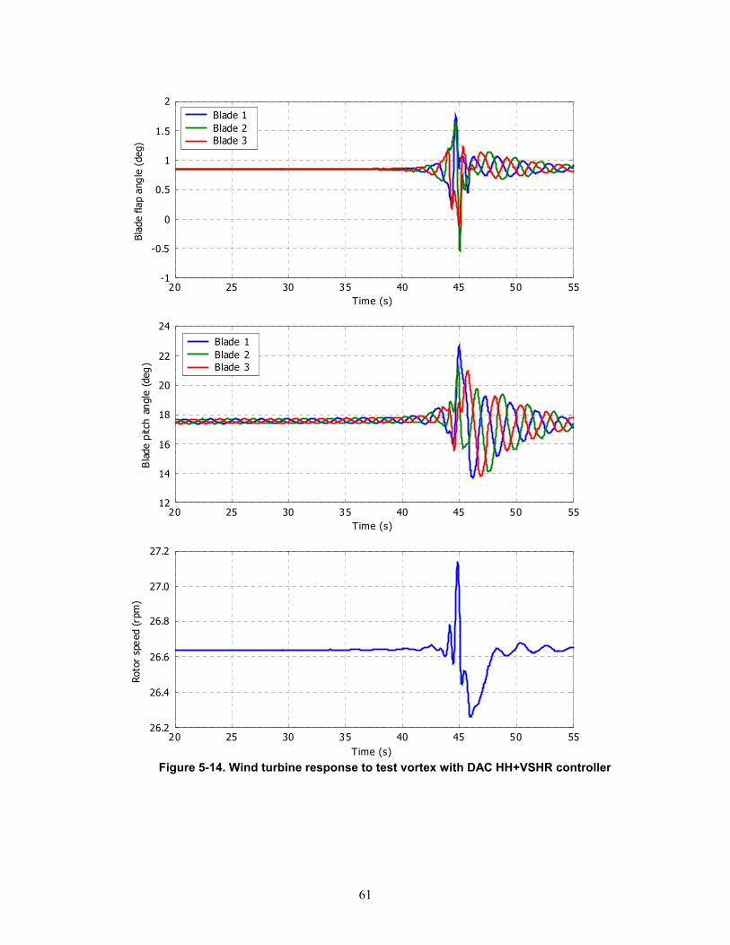
61

20 25 30 35 40 45 50 55-1

-0.5

0

0.5

1

1.5

2

Time (s)

Blad

e fla

p an

gle

(deg

)

Blade 1Blade 2Blade 3

20 25 30 35 40 45 50 5512

14

16

18

20

22

24

Time (s)

Bla

de p

itch

angl

e (d

eg)

Blade 1Blade 2Blade 3

20 25 30 35 40 45 50 5526.2

26.4

26.6

26.8

27.0

27.2

Time (s)

Roto

r sp

eed

(rpm

)

Figure 5-14. Wind turbine response to test vortex with DAC HH+VSHR controller

62

The blade flap states and state estimates are shown in Figure 5-15. The estimates follow the trend of the state, as desired. Figure 5-16 illustrates the estimated uniform wind speed, which remains at 18 m/s. The estimated rotor speed and the actual rotor speed, also shown in Figure 5-16, are very similar. This is expected because the rotor speed is a measurement input to the controller.

20 25 30 35 40 45 50 55-1

-0.5

0

0.5

1

Blad

e 1

flap

angl

e (d

eg)

T ime (s)20 25 30 35 40 45 50 55

-20

-10

0

10

20

Blad

e 1

flap

rate

(de

g/s)

Time (s)

20 25 30 35 40 45 50 55-1

-0.5

0

0.5

1

Blad

e 2

flap

angl

e (d

eg)

T ime (s)20 25 30 35 40 45 50 55

-20

-10

0

10

20

Blad

e 2

flap

rate

(de

g/s)

Time (s)

20 25 30 35 40 45 50 55-1

-0.5

0

0.5

1

Blad

e 3

flap

angl

e (d

eg)

T ime (s)20 25 30 35 40 45 50 55

-20

-10

0

10

20

Blad

e 3

flap

rate

(de

g/s)

Time (s)

StateEstimate

Figure 5-15. Blade states and state estimates for DAC HH+VSHR controller

63

20 25 30 35 40 45 50 5515

16

17

18

19

20

Time (s )

Win

d sp

eed

esti

mat

e (m

/s)

20 25 30 35 40 45 50 5526.2

26.4

26.6

26.8

27.0

27.2

Rot

or s

peed

(rpm

)

T ime (s )

StateEstimate

Figure 5-16. Wind speed estimate, rotor speed, and rotor speed estimate for DAC HH+VSHR

controller

Figure 5-17 shows the estimated sinusoidal variation in wind speed associated with the vertical shear profile. The wind speed associated with each blade tip is shown for comparison. The test vortex convects with a uniform wind (i.e., there is no vertical shear other than that induced by the vortex). However, the disturbance estimates do predict fluctuations that follow the trend of the velocity fluctuations associated with the vortex. As demonstrated in Figure 4-11, vertical shear is a good approximation of vortex passage, but it does not include the details of the vortex.

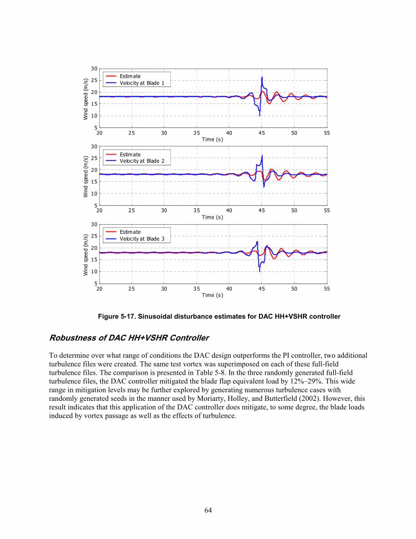
64

20 25 30 35 40 45 50 555

10

15

20

25

30

Time (s)

Win

d sp

eed

(m/s

)

20 25 30 35 40 45 50 555

10

15

20

25

30

Time (s)

Win

d sp

eed

(m/s

)

20 25 30 35 40 45 50 555

10

15

20

25

30

Time (s)

Win

d sp

eed

(m/s

) EstimateVeloc ity at Blade 3

EstimateVeloc ity at Blade 2

EstimateVeloc ity at Blade 1

Figure 5-17. Sinusoidal disturbance estimates for DAC HH+VSHR controller

Robustness of DAC HH+VSHR Controller To determine over what range of conditions the DAC design outperforms the PI controller, two additional turbulence files were created. The same test vortex was superimposed on each of these full-field turbulence files. The comparison is presented in Table 5-8. In the three randomly generated full-field turbulence files, the DAC controller mitigated the blade flap equivalent load by 12%–29%. This wide range in mitigation levels may be further explored by generating numerous turbulence cases with randomly generated seeds in the manner used by Moriarty, Holley, and Butterfield (2002). However, this result indicates that this application of the DAC controller does mitigate, to some degree, the blade loads induced by vortex passage as well as the effects of turbulence.

65

Table 5-8. Additional Comparisons of PI Controller and DAC HH+VSHR Controller Performance for Vortex Superimposed on Full-Field Turbulence

Turbulence + vortex (2) Turbulence + vortex (3)

PIDAC

HH+VSHR Difference PIDAC

HH+VSHR DifferenceRMS speed error (rpm) 0.34 0.34 -2% 0.34 0.27 -20%Max speed error (% rated) 2.5 2.4 -5% 2.1 1.9 -11%Max pitch rate (deg/s) 8.4 19.3 130% 11.3 24.3 116%RMS pitch rate (deg/s) 3.11 6.87 121% 2.93 6.89 135%Max pitch acceleration (deg/s^2) 50.6 109.8 117% 68.4 164.2 140%RMS pitch acceleration (deg/s^2) 11.74 25.35 116% 13.79 27.40 99%Flap damage equivalent load (kNm) 362 257 -29% 443 388 -12%Blade 1 RFB range (kNm) 539 378 -30% 661 474 -28%Blade 2 RFB range (kNm) 487 383 -21% 650 579 -11%Blade 3 RFB range (kNm) 476 367 -23% 653 524 -20%

The vortex parameters were then adjusted to determine the robustness of the DAC controller’s response to parameter variation. Table 5-9 shows the comparison between the DAC and PI controllers for five different vortex configurations, all with a mean convection speed of 18 m/s. The test vortex used in the DAC design is shown in the center. Again, the DAC controller mitigates blade loads as compared to the PI controller for all conditions. The margin decreases as the vortex radius decreases, and it remains relatively constant as circulation increases. The general trend in loads follows that of the surface shown in Figure 4-12. However, the maximum pitch rate exceeds the prescribed limit in most cases, and the maximum pitch acceleration is exceeded in two cases.

66

Table 5-9. Effect of Changing Radius and Circulation Strength of Vortex for DAC HH+VSHR Controller

R=15.7 m, G=-577 m^2/s

^ PIDAC

HH+VSHR DifferenceRMS speed error (rpm) 0.05 0.09 65%Max speed error (% rated) 1.0 1.4 41%Max pitch rate (deg/s) ^ 4.8 19.2 304%RMS pitch rate (deg/s) 0.67 3.30 394%Max pitch acceleration(deg/s^2) 25.6 65.6 156%RMS pitch acceleration (deg/s^2) ^ 4.10 11.53 181%Flap damage equivalent load (kNm) 344 280 -18%Blade 1 RFB range (kNm) ^ 447 300 -33%Blade 2 RFB range (kNm) 513 418 -18%Blade 3 RFB range (kNm) 420 346 -18%

^ R=10.7 m, G=-377 m^2/s R=10.7 m, G=-577 m^2/s R=10.7 m, G=-777 m^2/s

PIDAC

HH+VSHR Difference PIDAC

HH+VSHR Difference PIDAC

HH+VSHR DifferenceRMS speed error (rpm) 0.03 0.05 73% 0.05 0.08 68% 0.07 0.12 67%Max speed error (% rated) ^ 0.9 1.1 16% 1.6 1.9 14% 2.3 2.8 20%Max pitch rate (deg/s) 5.9 14.6 147% 9.9 23.5 138% 13.2 33.2 150%RMS pitch rate (deg/s) 0.64 1.87 193% 1.03 2.94 186% 1.31 4.03 207%Max pitch acceleration(deg/s^2) ^ 41.1 83.5 103% 67.7 136.4 101% 91.3 197.9 117%RMS pitch acceleration (deg/s^2) 5.06 9.39 86% 8.02 14.74 84% 10.10 20.28 101%Flap damage equivalent load (kNm) 223 203 -9% 369 336 -9% 473 433 -8%Blade 1 RFB range (kNm) 273 224 -18% 422 345 -18% 594 473 -20%Blade 2 RFB range (kNm) ^ 334 303 -9% 551 501 -9% 706 647 -8%Blade 3 RFB range (kNm) 252 228 -10% 381 334 -13% 493 470 -5%

^R=5.7 m, G=-577 m^2/s

PIDAC

HH+VSHR DifferenceRMS speed error (rpm) ^ 0.04 0.06 44%Max speed error (% rated) 1.6 1.8 10%Max pitch rate (deg/s) 10.4 21.2 105%RMS pitch rate (deg/s) ^ 1.03 2.14 107%Max pitch acceleration(deg/s^2) 88.8 183.0 106%RMS pitch acceleration (deg/s^2) 8.36 15.81 89%Flap damage equivalent load (kNm) ^ 384 375 -2%Blade 1 RFB range (kNm) 383 366 -4%Blade 2 RFB range (kNm) 573 560 -2%Blade 3 RFB range (kNm) ^ 259 241 -7%

R in

crea

sin

g

G increasing > > > > > > > Table 5-10 compares the DAC and PI controllers when the vortex center height is increased from the hub height to the top of the rotor. As shown in Figure 4-12, the load variation resulting from the vortex decreases substantially as the vortex center is raised above the hub. The DAC controller mitigates the blade loads as compared to the PI controller for each selected height. The margin decreases as the vortex center is raised, but again, the loads decrease in general.

67

Table 5-10. Effect of Changing Vortex Center Height with Respect to Hub for DAC HH+VSHR Controller

z increasing > > > > > > >

z=0 m z=11.0 m z=23 m

PIDAC

HH+VSHR Difference PIDAC

HH+VSHR Difference PIDAC

HH+VSHR DifferenceRMS speed error (rpm) 0.05 0.08 68% 0.15 0.12 -20% 0.26 0.25 -2%Max speed error (% rated) 1.6 1.9 14% 1.3 1.2 -6% 2.5 3.4 34%Max pitch rate (deg/s) 9.9 23.5 138% 6.0 11.1 84% 8.6 11.8 36%RMS pitch rate (deg/s) 1.03 2.94 186% 1.07 2.02 90% 1.86 2.19 18%Max pitch acceleration(deg/s^2) 67.7 136.4 101% 25.0 64.7 158% 20.9 37.4 79%RMS pitch acceleration (deg/s^2) 8.02 14.74 84% 2.92 8.01 174% 3.25 4.64 43%Flap damage equivalent load (kNm) 369 336 -9% 276 251 -9% 166 163 -2%Blade 1 RFB range (kNm) 422 345 -18% 412 374 -9% 248 243 -2%Blade 2 RFB range (kNm) 551 501 -9% 315 288 -9% 207 216 5%Blade 3 RFB range (kNm) 381 334 -13% 239 207 -13% 208 237 14%

Chapter Conclusions A baseline PI controller was designed for the three-blade turbine model to perform similarly to the PI controller implemented in the two-blade CART field experiment. All subsequent DAC designs were compared to this baseline controller. Multiple performance metrics were used to evaluate controller performance. The peak rotor speed, RMS of rotor speed error, pitch actuation rate and acceleration, blade root flap bending moment range, and damage equivalent load were all assessed as important criteria for controller performance. Several DAC designs were presented. Initially a disturbance model that included both u and w velocity components for 10 elements on each blade, resulting in 60 disturbance inputs, was created. An estimator could not be designed because the augmented system was not observable. However, implementation of this design as a FSFB controller indicated that as much as 30% blade load range and damage equivalent load reduction was possible. This was accomplished by commanding independent blade pitch angles in relation to the vortex velocity field. A simple DAC design using a single disturbance input of uniform wind speed did not command independent blade pitch angles and performed similarly to the PI controller. A DAC design using only the blade tip element velocities for a six-input disturbance model resulted in some load mitigation, but speed regulation was compromised. This disturbance model did not lead to adequate blade flap angle estimates and also commanded collective pitch angles. Finally, a DAC design that incorporated a uniform wind disturbance and two sinusoidal disturbances that approximated the azimuthally varying effect of vertical shear provided 9% damage equivalent load reduction when the vortex was input to the simulation.

This DAC design produced even greater damage equivalent load reduction over the PI controller when the vortex was superimposed on turbulent wind. The controller appears robust when the vortex radius and circulation strength are varied because the DAC produces lower blade damage equivalent loads than the PI controller. As the vortex is raised from hub height to the top of the rotor, the magnitude of the blade loads is reduced, and the margin of load reduction achieved by the DAC over the PI controller is also reduced.

The blade load conditions that lead to increased fatigue damage resulting from vortex passage are mitigated by implementation of a DAC controller. The disturbance is modeled as a uniform wind and an azimuthally varying vertical shear. The implementation of FSFB of a disturbance model that incorporates velocity changes at multiple points along the blade span indicates that even more blade load mitigation is possible.

68

Chapter 6

Conclusion to This Work and Beginning of Future Investigation

The wind turbine industry is poised for dramatic growth as turbines with diameters and hub heights approaching 100 m enter the market. These large rotating structures are expected to perform for 20 years or longer, but they encounter cyclic load fluctuations that cause fatigue damage. These loads mandate that the machines be heavier, more dynamically active, and thus more costly. These fatigue loads are further exacerbated by atmospheric flow phenomena that produce turbulence structures not modeled in today’s design codes. Advanced control algorithms offer an opportunity to extend fatigue lifetime while contributing to COE decreases through improved performance.

The diurnal cycle of the planetary boundary layer produces stability conditions in which coherent turbulence structures may develop, as discussed in Chapter 2. Various atmospheric phenomena, such as low-level jets, gravity waves, and Kelvin-Helmholtz instabilities, occur at heights where large wind turbines are expected to operate. These atmospheric phenomena are excellent sources of coherent turbulence on the same dimensional scale as these large machines.

As explained in Chapter 3, quantifying the effects of turbulence structures on wind turbines is difficult. Experimental data consisting of three-component wind velocity measurements at five locations corresponding to wind turbine dimensions furnished a unique opportunity to characterize these structures. Inflow and load data collected simultaneously from an operating wind turbine were used to establish a causal relationship between a blade flap fatigue load indicator and turbulence indicators. Sufficient measurements were made to provide some correlation between coherent turbulence and blade flap bending moments. The Reynolds stress measurements of the impinging wind indicated vorticity in the flow field. Complications arose from the wind turbine dynamics associated with the teetering hub and blade pitch control algorithm. However, the detrimental nature of the turbulence/wind turbine interaction was well documented.

In Chapter 4, the aerodynamic response of the wind turbine to a vortex was isolated using an analytic, Rankine vortex model in simulation with a rigid wind turbine model. The blade root flap bending moment range, which contributes to the fatigue damage equivalent load, was compared for vortices of various radius, circulation strength, orientation, plane of rotation, and height above the turbine hub. The experimental data were used to verify the magnitude of predicted loads with actual turbine measurements and to bound the vortex circulation strength. Rigid two- and three-blade wind turbines responded similarly to the range of vortex parameters. The vortex characteristics that contribute to fatigue damage were identified.

Chapter 5 presents an example of a DAC design that mitigates the blade flap fatigue equivalent load resulting from vortex passage as compared to a standard industry PI controller. This design models the wind disturbance as a uniform wind with a spatially varied vertical shear contribution. Other designs that did not incorporate enough detail of the vortex to reduce loads were presented as well. A disturbance model that incorporates wind velocities along the span of the blade was implemented in FSFB because observability conditions were not met. This simulation suggests that even greater fatigue load mitigation is possible if the vortex detail is modeled sufficiently.

69

The robustness of the successful DAC design was explored. The representative vortex was superimposed on three different, randomly generated turbulence files, and the DAC controller outperformed the PI controller in all three cases. Vortex parameter variation also yielded superior performance of the DAC over the PI controller. The uniform wind and vertical shear disturbance model apparently approximates the vortex flow field well enough to result in some blade load mitigation, which leads to extended blade fatigue life.

This report serves as a strong basis from which investigators can further pursue this important wind turbine issue. Several issues remain to be investigated before the complicated wind turbine/vortex interaction can be fully understood. Field testing is always the culmination of control design, and more tasks designed to ascertain the robustness of this DAC design must be completed. Additional investigation of the atmospheric conditions that produce and sustain vortices will lead to improved disturbance modeling. Continued simulation and development using the tools produced by this study will give greater insight into the appropriate vortex detail necessary to achieve the maximum load mitigation.

This control design was restricted to one operational regime, Region 3, and expansion to other operation regimes must be completed before field implementation. In addition, further study of the robustness to turbulence should be performed. Randomly selecting vortex size and strength parameters, along with the randomly selected turbulence seeds, provides the test engineer with greater confidence in the fidelity of the control algorithm before field implementation. Unmodeled modes in the control design have thwarted designers in the past. When a fully flexible wind turbine simulation is used with this 4 degree-of-freedom DAC controller, the tower fore-aft and drive-train torsion modes will probably become unstable (Wright 2003). However, Wright did show that these modes can be stabilized successfully. Once these issues are addressed, field testing can begin.

Improved understanding of the atmospheric phenomena that produce vortices will yield information that will enhance the disturbance model. Questions about the frequency of occurrence, the typical size, and the typical strength of the vortices remain unanswered. In addition, detection capability of inflow vortices could lead to advanced control designs that include measurements of the vortex.

Exploitation of the tools and results presented here could lead to more detailed vortex disturbance models that further mitigate blade loads. The aerodynamic response of the wind turbine blade to the impinging vortex must be understood on the blade element level. The spanwise variation of angle-of-attack and lift coefficient as the vortex passes may lead to additional parameters that can be modeled as disturbance inputs. For instance, the chord of the circle formed by the vortex core and its extent over the blade may be important. Perhaps additional measurements on the blade such as angle-of-attack or lift coefficient would deliver information that permits additional blade load mitigation to the controller.

One complicating issue is the assumption of linearity necessary for state-space design. The controller operates on perturbations from the operating point, so as to minimize or reject the difference to restore the plant to the operating point condition. The wind turbine operating point cannot have the vortex present because it is an intermittent phenomenon. However, to create the disturbance model, perturbations of the vortex parameters are required. To perturb from no vortex to the vortex centered on the rotor may violate the linearity assumption. This must be explored to augment the disturbance model with vortex parameters.

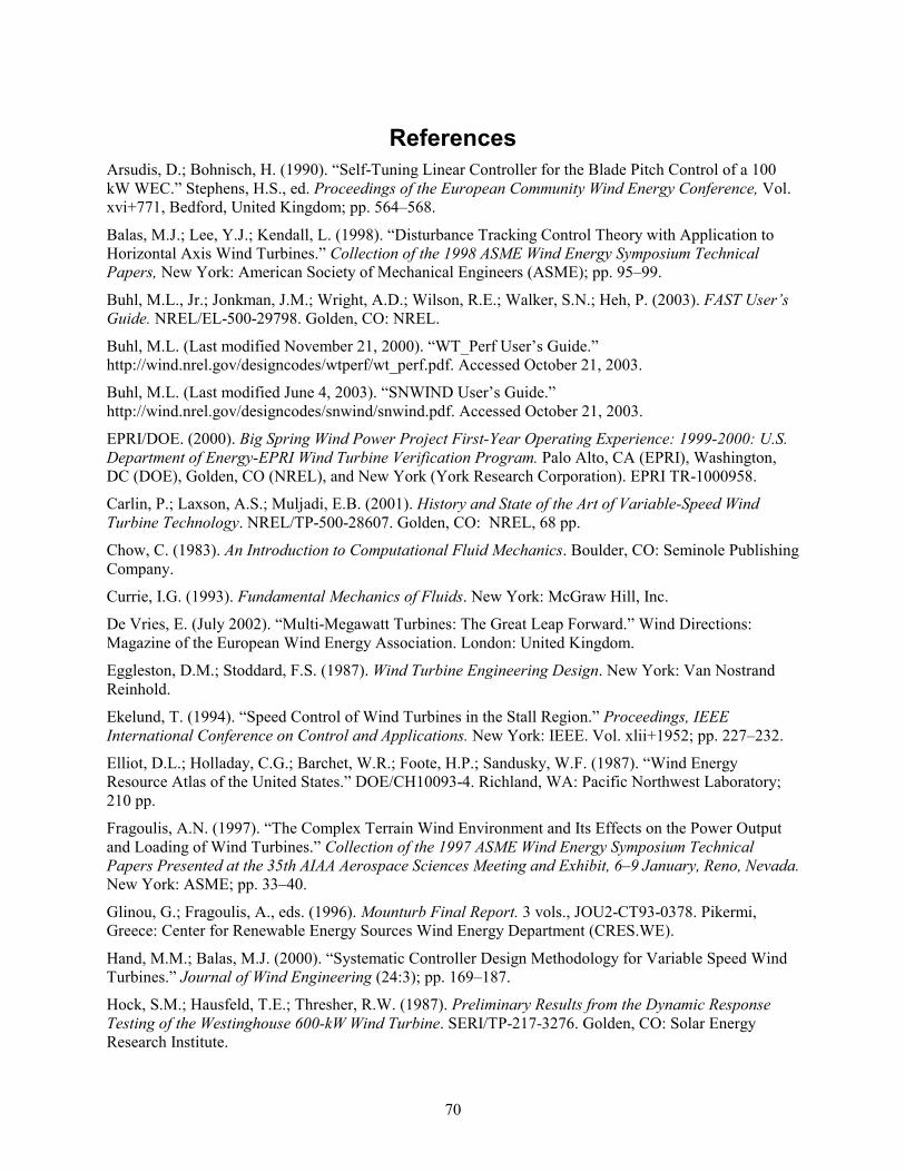
70

References Arsudis, D.; Bohnisch, H. (1990). “Self-Tuning Linear Controller for the Blade Pitch Control of a 100 kW WEC.” Stephens, H.S., ed. Proceedings of the European Community Wind Energy Conference, Vol. xvi+771, Bedford, United Kingdom; pp. 564–568.

Balas, M.J.; Lee, Y.J.; Kendall, L. (1998). “Disturbance Tracking Control Theory with Application to Horizontal Axis Wind Turbines.” Collection of the 1998 ASME Wind Energy Symposium Technical Papers, New York: American Society of Mechanical Engineers (ASME); pp. 95–99.

Buhl, M.L., Jr.; Jonkman, J.M.; Wright, A.D.; Wilson, R.E.; Walker, S.N.; Heh, P. (2003). FAST User’s Guide. NREL/EL-500-29798. Golden, CO: NREL.

Buhl, M.L. (Last modified November 21, 2000). “WT_Perf User’s Guide.” http://wind.nrel.gov/designcodes/wtperf/wt_perf.pdf. Accessed October 21, 2003.

Buhl, M.L. (Last modified June 4, 2003). “SNWIND User’s Guide.” http://wind.nrel.gov/designcodes/snwind/snwind.pdf. Accessed October 21, 2003.

EPRI/DOE. (2000). Big Spring Wind Power Project First-Year Operating Experience: 1999-2000: U.S. Department of Energy-EPRI Wind Turbine Verification Program. Palo Alto, CA (EPRI), Washington, DC (DOE), Golden, CO (NREL), and New York (York Research Corporation). EPRI TR-1000958.

Carlin, P.; Laxson, A.S.; Muljadi, E.B. (2001). History and State of the Art of Variable-Speed Wind Turbine Technology. NREL/TP-500-28607. Golden, CO: NREL, 68 pp.

Chow, C. (1983). An Introduction to Computational Fluid Mechanics. Boulder, CO: Seminole Publishing Company.

Currie, I.G. (1993). Fundamental Mechanics of Fluids. New York: McGraw Hill, Inc.

De Vries, E. (July 2002). “Multi-Megawatt Turbines: The Great Leap Forward.” Wind Directions: Magazine of the European Wind Energy Association. London: United Kingdom.

Eggleston, D.M.; Stoddard, F.S. (1987). Wind Turbine Engineering Design. New York: Van Nostrand Reinhold.

Ekelund, T. (1994). “Speed Control of Wind Turbines in the Stall Region.” Proceedings, IEEE International Conference on Control and Applications. New York: IEEE. Vol. xlii+1952; pp. 227–232.

Elliot, D.L.; Holladay, C.G.; Barchet, W.R.; Foote, H.P.; Sandusky, W.F. (1987). “Wind Energy Resource Atlas of the United States.” DOE/CH10093-4. Richland, WA: Pacific Northwest Laboratory; 210 pp.

Fragoulis, A.N. (1997). “The Complex Terrain Wind Environment and Its Effects on the Power Output and Loading of Wind Turbines.” Collection of the 1997 ASME Wind Energy Symposium Technical Papers Presented at the 35th AIAA Aerospace Sciences Meeting and Exhibit, 6–9 January, Reno, Nevada. New York: ASME; pp. 33–40.

Glinou, G.; Fragoulis, A., eds. (1996). Mounturb Final Report. 3 vols., JOU2-CT93-0378. Pikermi, Greece: Center for Renewable Energy Sources Wind Energy Department (CRES.WE).

Hand, M.M.; Balas, M.J. (2000). “Systematic Controller Design Methodology for Variable Speed Wind Turbines.” Journal of Wind Engineering (24:3); pp. 169–187.

Hock, S.M.; Hausfeld, T.E.; Thresher, R.W. (1987). Preliminary Results from the Dynamic Response Testing of the Westinghouse 600-kW Wind Turbine. SERI/TP-217-3276. Golden, CO: Solar Energy Research Institute.

71

Huyer, S.; Simms, D.; Robinson, M. (1996). “Unsteady Aerodynamics Associated with a Horizontal Axis Wind Turbine.” AIAA J., 34, No. 7, pp. 1410-1419.

IEA. (2002). “IEA Wind Energy Annual Report.” Boulder, CO: PWT Communications.

Johnson, C.D. (1976). “Theory of Disturbance Accommodating Controllers.” Leondes, C.T., ed. Control and Dynamic Systems; Advances Theory and Applications, Vol. 12. New York: Academic Press; pp. 387–489.

Kelley, N. (October 2001). Personal communication. Boulder, CO.

Kelley, N.; Hand, M.; Larwood, S.; McKenna, E. (2002). “The NREL Large-Scale Turbine Inflow and Response Experiment—Preliminary Results.” Collection of the 2002 ASME Wind Energy Symposium Technical Papers Presented at the 40th AIAA Aerospace Sciences Meeting and Exhibit, 14–17 January, Reno, Nevada. New York: ASME; pp. 412–426. Also published as NREL Report No. CP-500-30917, Golden, CO: NREL.

Kelley, N.D.; Bialasiewicz, J.T.; Osgood, R.M.; Jakubowski, A. (2000). “Using Wavelet Analysis to Assess Turbulence/Rotor Interactions.” Wind Energy (3:4); pp.121–134.

Kelley, N.D. (1994). “The Identification of Inflow Fluid Dynamics Parameters that can be Used to Scale Fatigue Loading Spectra of Wind Turbine Structural Components.” Musial, W., et al., eds. Proceedings, Wind Energy 1994. Solar Energy Division (SED)-Vol. 15. New York: ASME; pp. 181–196. Also published as NREL Report No. TP-442-6008, Golden, CO: NREL.

Kelley, N.D. (1992). Full Vector (3-D) Inflow Simulation in Natural and Wind Farm Environments Using an Expanded Version of the SNLWIND (VEERS) Turbulence Code. NREL/TP-442-5225. Prepared for the 12th ASME Wind Energy Symposium, January 1993. Golden, CO: NREL; 8 pp.

Kendall, L.; Balas, M.J.; Lee, Y.J.; and Fingersh, L.J. (1997). “Application of Proportional-Integral and Disturbance Accommodating Control to Variable-Speed Variable Pitch Horizontal Axis Wind Turbines.” Journal of Wind Engineering (12:1); pp. 21–38.

Kwakernaak, H.; Sivan, R. (1972). Linear Optimal Control Systems. New York: Wiley-Interscience.

Laino, D.J.; Hansen, A.C. (Last modified August 8, 2001). “User’s Guide to the Wind Turbine Aerodynamics Computer Software AeroDyn v.12.50.” http://wind.nrel.gov/designcodes/AeroDyn/AeroDyn.pdf. Accessed September 24, 2003.

Leithead, W.E.; de la Salle, S.; Reardon, D.; Grimble, M.J. (1991). “Wind Turbine Modelling and Control.” International Conference on Control, Conference Publication No. 332. London: IEE.

Malcolm, D.J.; Hansen, A.C. (2002). WindPACT Turbine Rotor Design Study: June 2000–June 2002. NREL/SR-500-32495. Golden, CO: NREL; 82 pp.

The Mathworks, Inc. (2002). MATLAB: The Language of Technical Computing User’s Manual, Version 6.5. Natick, MA: The Mathworks, Inc.

Mechanical Dynamics, Inc. (1998). Using ADAMS/Solver (v9.1). Ann Arbor, MI: Mechanical Dynamics, Inc.

Moriarty, P.J.; Holley, W.E.; Butterfield, C.P. (2002). “Probabilistic Methods for Predicting Wind Turbine Design Loads.” Collection of the 2003 Wind Energy Symposium Technical Papers Presented at the 41st AIAA Aerospace Sciences Meeting and Exhibit, 6–9 January, Reno, Nevada. New York: ASME; pp. 235–243.

Newsom, R.K.; Banta, R.M. (in press). “Shear-Instability Gravity Waves in the Stable Nocturnal Boundary Layer as Observed by Doppler Lidar CASES-99.” Journal of the Atmospheric Sciences.

72

Rice, R., ed. (1997). SAE Fatigue Design Handbook, 3rd edition. Warrendale, PA: Society of Automotive Engineers; 470 pp.

Robinson, M. (November 11, 2003). Personal communication. Boulder, CO.

Snow, A.L.; Heberling, C.F., II; Van Bibber, L.E. (1989). The Dynamic Response of a Westinghouse 600-kW Wind Turbine. SERI/STR-217-3405. Golden, CO: Solar Energy Research Institute.

Stol, K. (2001). “Dynamics Modeling and Periodic Control of Horizontal-Axis Wind Turbines.” Ph.D. thesis. Boulder, CO: University of Colorado.

Stol, K.; Bir, G. (Last modified July 15, 2003). “User’s Guide for SymDyn Version 1.2.” http://wind/designcodes/symdyn/symdyn.pdf. Accessed October 2, 2003.

Stol, K. (2003). “Disturbance Tracking and Blade Load Control of Wind Turbines in Variable-Speed Operation.” Collection of the 2003 ASME Wind Energy Symposium Technical Papers Presented at the 41st AIAA Aerospace Sciences Meeting and Exhibit, 6–9 January, Reno, Nevada. New York: ASME; pp. 317–322.

Stol, K.; Balas, M. (2002). “Periodic Disturbance Accommodating Control for Speed Regulation of Wind Turbines.” Collection of the 2002 ASME Wind Energy Symposium Technical Papers Presented at the 40th AIAA Aerospace Sciences Meeting and Exhibit, 14–17 January, Reno, Nevada. New York: ASME; pp. 310–315.

Stol, K.; Rigney, B.; Balas, M. (2000). “Disturbance Accommodating Control of a Variable-Speed Turbine Using a Symbolic Dynamics Structural Model.” Collection of the 2000 ASME Wind Energy Symposium Technical Papers Presented at the 38th AIAA Aerospace Sciences Meeting and Exhibit, 10–13 January, Reno, Nevada. New York: ASME; pp. 84-90.

Stuart, J.G.; Wright, A.D.; and Butterfield, C. P. (1996). Considerations for an Integrated Wind Turbine Controls Capability at the National Wind Technology Center: An Aileron Control Case Study for Power Regulation and Load Mitigation. NREL/TP-440-21335. Golden, CO: NREL.

Stull, R.B. (1988). An Introduction to Boundary Layer Meteorology. Dordrecht, The Netherlands: Kluwer Academic Publishers.

Sutherland, H.J.; Kelley, N.D.; Hand, M.M. (2003). “Inflow and Fatigue Response of the NWTC Advanced Research Turbine.” Collection of the 2003 ASME Wind Energy Symposium Technical Papers Presented at the 41st AIAA Aerospace Sciences Meeting and Exhibit, 6-9 January, Reno, Nevada. New York: ASME; pp. 214–224.

Sutherland, H. (2002). “Inflow and the Fatigue of the LIST Wind Turbine.” Collection of the 2002 ASME Wind Energy Symposium Technical Papers Presented at the 40th AIAA Aerospace Sciences Meeting and Exhibit, 14-17 January, Reno, Nevada. New York: ASME; pp. 427–437.

Tangler, J.; Smith, B.; Jager, D.; Olsen, T. (1990). “SERI Thin-Airfoil Blade Atmospheric Performance Test: Final Results.” Windpower '90: Proceedings of the Conference held 24-28 September 1990, Washington, DC. Washington, DC: American Wind Energy Association; pp. 118-125. Also published as NREL Report No. TP-257-4076, Golden CO: NREL.

Wilson, R.E.; Freeman, L.N.; Walker, S.N.; Harman, C.R. (1996). Final Report for the FAST Advanced Dynamics Code: Two Bladed Teetered Hub Version 2.4 User's Manual Appendix for Three and Four Bladed Versions. Also published as NREL Report No. SR-500-23563, Golden, CO: NREL; 51 pp.

Wright, A. (2003). Modern Control Design for Flexible Wind Turbines. Ph.D. thesis. Boulder, CO: University of Colorado.

73

Appendix A

Vortex Flow-Field Model Derivation and Implementation A Rankine vortex model was used to simulate vortices of varied parameters in the flow field upwind of the wind turbine. The vortex itself is assumed to behave like a solid body, rotating cylinder of infinite length surrounded by an inviscid and incompressible flow field that is modeled with potential flow vortex equations. The convection speed, radius, circulation strength, and Cartesian coordinates of the vortex center are variable. Equations were developed for vortices in three planes. Linear superposition of a uniform flow with the vortex is used to cause the vortex to convect through the wind turbine rotor.

The coordinate system is aligned with the one used by the aerodynamics subroutines within AeroDyn, the wind turbine dynamics code that computes the aerodynamic forces on blade elements (Laino and Hansen 2001). The wind flows from negative x toward positive x as illustrated in Figure 4-1. The y-axis is positive to the left when looking downwind, and the z-axis is positive vertically as shown in Figure 4-2. The origin is located at the intersection of the undeflected hub height of the wind turbine and the tower centerline. AeroDyn was modified to include a new subroutine called USERWIND. The x, y, and z coordinates of a blade element are passed to the subroutine; the corresponding u, v, and w velocity components are computed and returned to the main program.

Figure A-1 shows the coordinate system of a vortex centered at the origin. The cylindrical coordinates of the Rankine vortex can be described as

ruuR πθ 2

;0 Γ== (A-1)

using a complex potential (Currie 1993) or the Biot-Savart law (Chow 1983). The velocity along the axis of the vortex is also zero. The relationship between the circulation strength and the vorticity is described by the following equation:

ωπω 22 rdAnA

=⋅=Γ ∫ (A-2)

x

z

uθ

urwu

r

θ

ω

Figure A-1. Coordinate system of vortex rotating in XZ plane

74

The equations describing a vortex in the XZ plane are developed below using the vortex center as the origin of the coordinate system. Similar equations were developed for vortices rotating in the YZ and XY planes. The vortex is radius R; it convects at ∞V ; the circulation strength is Γ; and the vorticity is ω. The velocity components are converted to Cartesian coordinates for compatibility with the aerodynamics subroutines.

For a potential flow vortex in the XZ plane, (r > R):

wuuuU r +=+= θ (A-3)

+Γ−

=Γ−

=−= 222sin

2sincos

zxz

ruuu r π

θπ

θθ θ

(A-4)

+Γ

=Γ

=+= 222cos

2cossin

zxx

ruuw r π

θπ

θθ θ (A-5)

For the vortex core, which is approximated by solid body rotation (r <= R):

wuuuU r +=+= θ (A-6)

ωθωθθ θ zruuu r −=−=−= sinsincos (A-7)

ωθωθθ θ xruuw r ==+= coscossin (A-8)

For a uniform flow field (all r):

∞= Vu (A-9)

If the vortex center is (x0, y0, z0) in the aerodynamics code coordinate system, and the coordinates provided by the aerodynamics subroutine are (x, y, z), the following equations describe the vortex rotating clockwise in the XZ plane for the vortex core (r <= R):

∞+−−= Vzzu )( 0 (A-10)

0=v (A-11)

ω)( 0xxw −= (A-12)

The following equations represent the velocity components for the potential flow surrounding the vortex (r > R):

∞+

−+−

−Γ−= V

zzxxzzu

o2

02

0

)()(2π (A-13)

75

0=v (A-14)

−+−

−Γ= 2

02

0 )()(2 zzxxxxw o

π (A-15)

Note that the x-coordinate of the vortex center, x0, moves tV ∆∞ * every time step. This allows the vortex to convect through the rotor. A clockwise rotating vortex core (r <= R) in the XY plane is described as follows:

∞+−= Vyyu )( 0 (A-16)

ω)( 0xxv −−= (A-17)

0=w (A-18)

The velocity components for the potential flow field surrounding the vortex (r > R) are listed below.

∞+

−+−

−Γ= V

yyxxyyu

o2

02

0

)()(2π (A-19)

−+−

−Γ−= 2

02

0 )()(2 yyxxxxv o

π (A-20)

0=w (A-21)

Again, the x-coordinate of the vortex center, x0, moves tV ∆∞ * every time step to convect through the rotor. A clockwise rotating vortex core (r <= R) in the YZ plane is described as follows:

∞= Vu (A-22)

ω)( 0zzv −−= (A-23)

ω)( 0yyw −= (A-24)

The velocity components for the potential flow field surrounding the vortex (r > R) are listed below.

∞= Vu (A-25)

∞+

−+−

−Γ−= V

zzyyzzv

o2

02

0

)()(2π (A-26)

76

−+−

−Γ= 2

02

0 )()(2 zzyyyyw o

π (A-27)

In this case, the vortex convects through the rotor by shifting y0 by tV ∆∞ * at every time step so that the vortex convects laterally across the rotor.

Vortex Superimposed on Turbulent Wind Field A grid of three component wind velocities corresponding to (x, y, z) positions was created using the SNWind code (Kelley 1992, Buhl 2003). The mean wind speed was specified to be 18 m/s and the turbulence intensity B. A MATLAB© (The Mathworks, Inc. 2002) script was created to read this binary wind file format, compute the vortex velocity components at each grid point location, add the vortex velocity components to the turbulent wind file velocity components, and output a new wind file that contains the vortex superimposed on the turbulent wind file. The aerodynamics code reads this file and interpolates between grid points to obtain the three velocity components at each blade element in order to compute the aerodynamic force coefficients on the blade.

Exhibit A-1. Example SNWIND input file

SNWind v1.2 input file for 18 m/s convection. Runtime options: 143456 First random seed (1-999999999) 789032 Second random seed (1-999999999) False Output hub-height turbulence parameters in GenPro-binary form? (Generates RootName.bin) False Output hub-height turbulence parameters in formatted form? (Generates RootName.dat) False Output hub-height time-series data in AeroDyn form? (Generates RootName.hh) True Output full-field time-series data in AeroDyn form? (Generates RootName.wnd, RootName.ddd) False Output full-field time-series data in formatted (readable) form? (Generates RootName.u, RootName.v, RootName.w) False Clockwise rotation looking downwind? (used only for full-field binary files) Turbine/model specifications: 6 Square grid-point matrix dimension (even values only) 0.05 Time step [seconds] 55.0 Usable length of time series [seconds] (program will add GridWidth/MeanHHWS seconds) 36.85 Hub height [m] (should be > 0.5*GridWidth) 60.00 Grid width and height [m] (should be >= 2*(RotorRadius+ShaftLength)) 0.0 Vertical mean flow (uptilt) angle [degrees] 0.0 Horizontal mean flow (skew) angle [degrees] Meteorological boundary conditions: "IECKAI" Turbulence model ("IECKAI"=Kaimal, "IECVKM"=Von Karman) "B" IIEC turbulence characteristic ("A", "B", or the turbulence intensity in percent) 36.85 Height of the reference wind speed [m] 18.0 Mean wind speed at the reference height [m/s] ================================================== NOTE: Do not add or remove any lines in this file!

Exhibit A-2. MATLAB© script, combine_turb_vortex.m, which superimposes vortex on full-field turbulence

% this script reads a binary full-field wind input file. It assumes that % dimensions and scaling are appropriate, i.e. no error checking. % % this must be entered from the *.sum file output from SNWind % TI(1)=15.5; % for V_18_turb.wnd % TI(2)=13.; % TI(3)=7.1; % % this must be entered from the *.sum file output from SNWind

77

% TI(1)=10.5; % for V_18_turbB.wnd % TI(2)=10.0; % TI(3)=7.0; % % this must be entered from the *.sum file output from SNWind % TI(1)=13.4; % for V_18_turbB2.wnd % TI(2)=10.7; % TI(3)=6.9; % this must be entered from the *.sum file output from SNWind TI(1)=14.5; % for V_18_turbB3.wnd TI(2)=12.9; TI(3)=7.1; filename='V_18_turbB3_XZ_CC_r_10_7_G_577'; % fid=fopen('V_18_turb_XZ_CC_r_10_7_G_577.wnd','r'); fid=fopen('V_18_turbB3.wnd','r'); header=fread(fid,19,'int16'); % Compute scaling values from header entries NFFComp=-header(1); FFZDelt=0.001*header(2); InvFFZD=1.0/FFZDelt; FFYDelt=0.001*header(3); InvFFYD=1.0/FFYDelt; FFXDelt=0.001*header(4); TFFSteps=2*header(5); XGrid=0.0; MeanFFWS=0.1*header(6); InvMFFWS=1.0/MeanFFWS; FFDTime=FFXDelt/MeanFFWS; FFRate=1.0/FFDTime; NZGrids=header(12)/1000.; FFZHWid=0.5*FFZDelt*(NZGrids-1); NYGrids=header(13)/1000.; FFYHWid=0.5*FFYDelt*(NYGrids-1); ZGrid = FFZDelt*(NZGrids-1)/2; YGrid = FFYDelt*(NYGrids-1)/2; DYGrid = FFYDelt; DZGrid = FFZDelt; % read u,v,w information at each time step u=zeros(NZGrids,NYGrids,TFFSteps); v=u; w=u; % XZ vortex parameters R_Vortex=10.7; X_Vortex=-810.0-(2*23+3.858); Y_Vortex=0; Z_Vortex=0; VS = -0.477; R_Turbine=23; HHWindSpeed=18; CIRC = VS*2*pi*R_Vortex*HHWindSpeed; VORT = CIRC/(2*pi*R_Vortex^2); for IT=1:TFFSteps ZGrid = -FFZDelt*(NZGrids-1)/2; for IR=1:NZGrids YGrid = -FFYDelt*(NYGrids-1)/2; for IC=1:1:NYGrids %assume anti-clockwise temp=fread(fid,1,'int16'); u(IR,IC,IT)=MeanFFWS*(1+0.00001*TI(1)*temp); temp=fread(fid,1,'int16'); v(IR,IC,IT)=0.00001*TI(2)*MeanFFWS*temp; temp=fread(fid,1,'int16'); w(IR,IC,IT)=0.00001*TI(3)*MeanFFWS*temp; % add vortex components R_Point = sqrt((XGrid-X_Vortex)^2 + (ZGrid-Z_Vortex)^2); if ( R_Point < R_Vortex ) u(IR,IC,IT) = u(IR,IC,IT)-VORT*(ZGrid-Z_Vortex); v(IR,IC,IT) = v(IR,IC,IT)+0.0; w(IR,IC,IT) = w(IR,IC,IT)+VORT*(XGrid-X_Vortex); else

78

u(IR,IC,IT) = u(IR,IC,IT)-CIRC/(2*pi)*(ZGrid-Z_Vortex)/((XGrid-X_Vortex)^2+(ZGrid-Z_Vortex)^2); v(IR,IC,IT) = v(IR,IC,IT)+0.0; w(IR,IC,IT) = w(IR,IC,IT)+CIRC/(2*pi)*(XGrid-X_Vortex)/((XGrid-X_Vortex)^2+(ZGrid-Z_Vortex)^2); end YGrid = YGrid + DYGrid; end ZGrid = ZGrid + DZGrid; end X_Vortex = X_Vortex + HHWindSpeed*FFDTime; end fclose(fid); % binary output file ifile=strcat(char(filename),'.wnd'); fid=fopen(ifile,'w'); fwrite(fid,header, 'int16'); % output u,v,w, data for IT=1:TFFSteps for IR=1:NZGrids for IC=1:NYGrids fwrite(fid,100000/TI(1)*(u(IR,IC,IT)/MeanFFWS-1),'int16'); fwrite(fid,100000/(MeanFFWS*TI(2))*v(IR,IC,IT),'int16'); fwrite(fid,100000/(MeanFFWS*TI(3))*w(IR,IC,IT),'int16'); end end end fclose(fid);

FORTRAN Code for Vortex Calculations and Sample Input File

Exhibit A-3. USERWIND.FOR subroutine

! ****************************************************** SUBROUTINE UserWind ! This subroutine gets XGRND,YGRND,ZGRND and TIME from ! MODULES FFWIND, and AeroTime. It assumes that ! XGRND is positive downwind, YGRND is positive left when ! looking downwind, and ZGRND is positive up. VX, VY, ! and VZ are computed, and UWmeanU, UWmeanV and UWmeanW are ! computed as well. These are declared in WIND. The hub ! height (HH) is declared in Rotor. DT is in AeroTime USE WIND USE FF_WIND USE AeroTime USE Rotor USE AD_IOParams ! UnWind USE Constant ! PI USE Blade ! IBLADE USE Element IMPLICIT NONE LOGICAL(1), SAVE :: FrstPass = .TRUE. ! Flag to indicate if this is the first pass. REAL HHWindSpeed, UW_U, UW_V, UW_W, PowerExp, VSlope, L,EndTime REAL XGrid, YGrid, DYGrid, ZGrid, DZGrid,OutX(55,55),OutY(55,55),OutZ(55,55) REAL R_Vortex, X_Vortex, Y_Vortex, Z_Vortex, CIRC, VORT, R_Point, VS REAL ElemArray(200), BladeArray(200) ! for output of blade element velocity data REAL Uop, Vop, Wop, Pert_Value INTEGER*2 TEMP1 DOUBLE PRECISION PREVTIME INTEGER IOS, GS, UnWindOut, IR, IC, IREC, Kelem INTEGER Pert_Blade, Pert_Elem CHARACTER*1 Pert_Comp CHARACTER*140 Frmt CHARACTER*150 LINE

79

CHARACTER*80 TITLE CHARACTER*110 MESAGE CHARACTER*10 FField LOGICAL WindOut, PrintFlag DATA UnWindOut /95/ ! Open the wind input file IF (FrstPass) THEN CALL OpenInputFile (UnWind, 'userwind.ipt', 'FORMATTED') ! Read in the title line READ(UnWind,'( A )',IOSTAT=IOS) TITLE IF ( IOS < 0 ) CALL PremEOF ( 'userwind.ipt' , 'Title' ) MESAGE = TITLE Frmt = '(''Heading of the userwind.ipt file :'', /A)' ! Read in the time length of the simulation; use 0 to signify no x_vortex movement READ(UnWind,'( A )',IOSTAT=IOS) LINE IF ( IOS < 0 ) CALL PremEOF ( 'userwind.ipt' , 'simulation time' ) READ(LINE,*,ERR=205) EndTime PREVTIME = 0.000 ! Read in the output file parameters READ(UnWind,'( A )',IOSTAT=IOS) LINE IF ( IOS < 0 ) CALL PremEOF ( 'userwind.ipt' , 'output file parameter' ) LINE = ADJUSTL( LINE ) CALL Conv2UC(LINE(1:5)) IF (LINE(1:4) == 'TRUE') THEN WindOut=.TRUE. PrintFlag=.FALSE. ! don't want to print until complete time step passes ! Read in the number of output grid nodes READ(UnWind,'( A )',IOSTAT=IOS) LINE IF ( IOS < 0 ) CALL PremEOF ( 'userwind.ipt' , 'grid size' ) READ(LINE,*,ERR=205) GS ! Read in the output grid dimension READ(UnWind,'( A )',IOSTAT=IOS) LINE IF ( IOS < 0 ) CALL PremEOF ( 'userwind.ipt' , 'grid dimension' ) READ(LINE,*,ERR=205) L XGrid = 0.0 ! if matching to turbine data is necessary change to be initial XGRND YGrid = L/2 ZGrid = L/2 DYGrid = L/(GS-1) DZGrid = L/(GS-1) ! Read in the hub-height wind speed READ(UnWind,'( A )',IOSTAT=IOS) LINE IF ( IOS < 0 ) CALL PremEOF ( 'userwind.ipt' , 'hub-height wind speed' ) READ(LINE,*,ERR=205) HHWindSpeed ! Open the output file and write binary header (in FFfile format) OPEN( UnWindOut , FILE='userwind.out' , STATUS='UNKNOWN', FORM='BINARY', ACCESS='DIRECT',RECL=2 ) WRITE (UnWindOut,REC= 1) INT2( -3 ) WRITE (UnWindOut,REC= 2) INT2( 1000.0*L/REAL(GS-1) ) WRITE (UnWindOut,REC= 3) INT2( 1000.0*L/REAL(GS-1) ) WRITE (UnWindOut,REC= 4) INT2( 1000.0*DTAero*HHWindSpeed ) WRITE (UnWindOut,REC= 5) INT2( (EndTime/DTAero)/2 ) WRITE (UnWindOut,REC= 6) INT2( 10.0*HHWindSpeed ) WRITE (UnWindOut,REC= 7) INT2( 0 ) WRITE (UnWindOut,REC= 8) INT2( 0 ) WRITE (UnWindOut,REC= 9) INT2( 0 ) WRITE (UnWindOut,REC=10) INT2( 0 ) WRITE (UnWindOut,REC=11) INT2( 0 ) WRITE (UnWindOut,REC=12) INT2( 1000*GS ) WRITE (UnWindOut,REC=13) INT2( 1000*GS ) WRITE (UnWindOut,REC=14) INT2( 0 ) WRITE (UnWindOut,REC=15) INT2( 0 ) WRITE (UnWindOut,REC=16) INT2( 0 ) WRITE (UnWindOut,REC=17) INT2( 0 ) WRITE (UnWindOut,REC=18) INT2( 0 ) WRITE (UnWindOut,REC=19) INT2( 0 ) IREC=20 OPEN (98,FILE='time.out')

80

! WRITE(98,'(2F15.5)') TIME, PREVTIME ELSE WindOut=.FALSE. PrintFlag = .FALSE. ! Skip the number of output grid nodes READ(UnWind,'( A )',IOSTAT=IOS) LINE IF ( IOS < 0 ) CALL PremEOF ( 'userwind.ipt' , 'grid size' ) READ(LINE,*,ERR=205) GS ! Skip the output grid dimension READ(UnWind,'( A )',IOSTAT=IOS) LINE IF ( IOS < 0 ) CALL PremEOF ( 'userwind.ipt' , 'uniform U' ) READ(LINE,*,ERR=205) L ! Read in the hub-height wind speed READ(UnWind,'( A )',IOSTAT=IOS) LINE IF ( IOS < 0 ) CALL PremEOF ( 'userwind.ipt' , 'hub-height wind speed' ) READ(LINE,*,ERR=205) HHWindSpeed ENDIF ! Read in the flow field type READ(UnWind,'( A )',IOSTAT=IOS) LINE IF ( IOS < 0 ) CALL PremEOF ( 'userwind.ipt' , 'flow field model' ) LINE = ADJUSTL( LINE ) CALL Conv2UC(LINE(1:7)) IF (LINE(1:7) == 'UNIFORM') THEN FField='UNIFORM' ! Read in the uniform U velocity READ(UnWind,'( A )',IOSTAT=IOS) LINE IF ( IOS < 0 ) CALL PremEOF ( 'userwind.ipt' , 'uniform U' ) READ(LINE,*,ERR=205) UW_U ! Read in the uniform V velocity READ(UnWind,'( A )',IOSTAT=IOS) LINE IF ( IOS < 0 ) CALL PremEOF ( 'userwind.ipt' , 'uniform V' ) READ(LINE,*,ERR=205) UW_V ! Read in the uniform W velocity READ(UnWind,'( A )',IOSTAT=IOS) LINE IF ( IOS < 0 ) CALL PremEOF ( 'userwind.ipt' , 'uniform W' ) READ(LINE,*,ERR=205) UW_W ELSEIF (LINE(1:5) == 'POWER') THEN FField='POWER' ! Read in the power law exponent READ(UnWind,'( A )',IOSTAT=IOS) LINE IF ( IOS < 0 ) CALL PremEOF ( 'userwind.ipt' , 'power law exponent' ) READ(LINE,*,ERR=205) PowerExp ELSEIF (LINE(1:6) == 'VLINSH') THEN FField='VLINSH' ! Read in the linear shear slope READ(UnWind,'( A )',IOSTAT=IOS) LINE IF ( IOS < 0 ) CALL PremEOF ( 'userwind.ipt' , 'vertical shear slope' ) READ(LINE,*,ERR=205) VSlope ELSEIF (LINE(3:6) == 'VRTX') THEN IF (LINE(1:2) == 'YZ') THEN FField='YZVRTX' ELSEIF (LINE(1:2) == 'XZ') THEN FField='XZVRTX' ELSEIF (LINE(1:2) == 'XY') THEN FField='XYVRTX' ENDIF ! Read in the vortex radius READ(UnWind,'( A )',IOSTAT=IOS) LINE IF ( IOS < 0 ) CALL PremEOF ( 'userwind.ipt' , 'vortex radius' ) READ(LINE,*,ERR=205) R_vortex ! Read in the x-coordinate vortex center READ(UnWind,'( A )',IOSTAT=IOS) LINE IF ( IOS < 0 ) CALL PremEOF ( 'userwind.ipt' , 'vortex x-coordinate' ) READ(LINE,*,ERR=205) X_Vortex ! Read in the y-coordinate vortex center READ(UnWind,'( A )',IOSTAT=IOS) LINE

81

IF ( IOS < 0 ) CALL PremEOF ( 'userwind.ipt' , 'vortex y-coordinate' ) READ(LINE,*,ERR=205) Y_Vortex ! Read in the z-coordinate vortex center READ(UnWind,'( A )',IOSTAT=IOS) LINE IF ( IOS < 0 ) CALL PremEOF ( 'userwind.ipt' , 'vortex z-coordinate' ) READ(LINE,*,ERR=205) Z_Vortex ! Read in the vortex rotational direction, fraction of HHWindSpeed READ(UnWind,'( A )',IOSTAT=IOS) LINE IF ( IOS < 0 ) CALL PremEOF ( 'userwind.ipt' , 'vortex sign' ) READ(LINE,*,ERR=205) VS CIRC = VS*2*PI*R_Vortex*HHWindSpeed VORT = VS*HHWindSpeed/R_Vortex Kelem = 1 ! for use in outputting blade element velocity data ELSEIF (LINE(1:7) == 'PERTURB') THEN FField = 'PERTURB' ! Read in the operating point READ (UnWind,'(A)',IOSTAT=IOS) LINE IF ( IOS < 0 ) CALL PremEOF ( 'userwind.ipt' , 'U operating point' ) READ(LINE,*,ERR=205) Uop READ (UnWind,'(A)',IOSTAT=IOS) LINE IF ( IOS < 0 ) CALL PremEOF ( 'userwind.ipt' , 'V operating point' ) READ(LINE,*,ERR=205) Vop READ (UnWind,'(A)',IOSTAT=IOS) LINE IF ( IOS < 0 ) CALL PremEOF ( 'userwind.ipt' , 'W operating point' ) READ(LINE,*,ERR=205) Wop ! Read in Blade, Element and Component perturbation location READ (UnWind,'(A)',IOSTAT=IOS) LINE IF ( IOS < 0 ) CALL PremEOF ( 'userwind.ipt' , 'Blade to be perturbed' ) READ(LINE,*,ERR=205) Pert_Blade READ (UnWind,'(A)',IOSTAT=IOS) LINE IF ( IOS < 0 ) CALL PremEOF ( 'userwind.ipt' , 'Element to be perturbed' ) READ(LINE,*,ERR=205) Pert_Elem READ (UnWind,'(A)',IOSTAT=IOS) LINE IF ( IOS < 0 ) CALL PremEOF ( 'userwind.ipt' , 'Component to be perturbed' ) LINE = ADJUSTL( LINE ) CALL Conv2UC(LINE(1:1)) Pert_Comp=LINE(1:1) ! Read in perturbation value READ (UnWind,'(A)',IOSTAT=IOS) LINE IF ( IOS < 0 ) CALL PremEOF ( 'userwind.ipt' , 'Perturbation value' ) READ(LINE,*,ERR=205) Pert_Value Kelem=1 ! for use in outputting perturbation velocity data for error checking ENDIF CLOSE ( UnWind ) FrstPass = .FALSE. ! These are required for the skewed wake correction. For now they are assumed ! to represent the mean convection speed which does not change with time. If ! time varying mean convection speed is needed, these can be updated in the ! other branch of the subroutine. These variables are declared in Module WIND. UWmeanU = HHWindSpeed UWmeanV = 0. UWmeanW = 0. RETURN ENDIF ! Compute VX, VY, and VZ using the ground coordinates (origin at hub-height). IF (EndTime.NE.0.0) THEN !for linearization, X_Vortex does not change IF ((FFIELD=='XZVRTX').OR.(FFIELD=='PERTURB')) THEN IF (Kelem.gt.(NB*NELM*2)) PrintFlag=.TRUE. IF (PREVTIME.NE.TIME) THEN X_Vortex = X_Vortex + HHWindSpeed*(TIME-PREVTIME) PREVTIME = TIME ENDIF

82

ELSEIF (PREVTIME.NE.TIME) THEN X_Vortex = X_Vortex + HHWindSpeed*(TIME-PREVTIME) ! XGrid = XGrid - (HHWindSpeed*(TIME-PREVTIME)) IF ( FField.EQ.'YZVRTX') THEN Y_Vortex = Y_Vortex + HHWindSpeed*(TIME - PREVTIME) ENDIF PREVTIME = TIME PrintFlag = .TRUE. ENDIF ENDIF SELECT CASE (FField) CASE ('UNIFORM') VX = UW_U VY = UW_V VZ = UW_W CASE ('POWER') VX = HHWindSpeed / HH**PowerExp * (ZGRND + HH)**PowerExp VY = 0 VZ = 0 CASE ('VLINSH') VX = (ZGRND) / VSlope + HHWindSpeed VY = 0 VZ = 0 CASE ('YZVRTX') R_Point = SQRT((YGRND-Y_Vortex)**2 + (ZGRND-Z_Vortex)**2) IF ( R_Point.LE.R_Vortex ) THEN VX = HHWindSpeed VY = -VORT*(ZGRND-Z_Vortex) VZ = VORT*(YGRND-Y_Vortex) ELSE VX = HHWindSpeed VY = -CIRC/(2*PI)*(ZGRND-Z_Vortex)/((YGRND-Y_Vortex)**2+(ZGRND-Z_Vortex)**2) VZ = CIRC/(2*PI)*(YGRND-Y_Vortex)/((YGRND-Y_Vortex)**2+(ZGRND-Z_Vortex)**2) ENDIF CASE ('XZVRTX') R_Point = SQRT((XGRND-X_Vortex)**2 + (ZGRND-Z_Vortex)**2) IF ( R_Point.LE.R_Vortex ) THEN VX = -VORT*(ZGRND-Z_Vortex) + HHWindSpeed VY = 0.0 VZ = VORT*(XGRND-X_Vortex) ELSE VX = -CIRC/(2*PI)*(ZGRND-Z_Vortex)/((XGRND-X_Vortex)**2+(ZGRND-Z_Vortex)**2)+HHWindSpeed VY = 0.0 VZ = CIRC/(2*PI)*(XGRND-X_Vortex)/((XGRND-X_Vortex)**2+(ZGRND-Z_Vortex)**2) ENDIF ! Currently XZ is only one capable of recording element velocity data IF (WindOut) THEN ElemArray(Kelem)=VX ElemArray(Kelem+1)=VZ BladeArray(Kelem)=IBlade BladeArray(Kelem+1)=JElem Kelem=Kelem+2 ENDIF CASE ('XYVRTX') R_Point = SQRT((YGRND-Y_Vortex)**2 + (XGRND-X_Vortex)**2) IF ( R_Point.LE.R_Vortex ) THEN VX = VORT*(YGRND-Y_Vortex)+HHWindSpeed VY = -VORT*(XGRND-X_Vortex) VZ = 0.0 ELSE VX = CIRC/(2*PI)*(YGRND-Y_Vortex)/((YGRND-Y_Vortex)**2+(XGRND-X_Vortex)**2)+HHWindSpeed VY = -CIRC/(2*PI)*(XGRND-X_Vortex)/((YGRND-Y_Vortex)**2+(XGRND-X_Vortex)**2) VZ = 0.0 ENDIF CASE ('PERTURB') IF ((IBlade==Pert_Blade).AND.(JElem==Pert_Elem)) THEN IF(Pert_Comp=='U') THEN VX = Pert_Value VY = Vop VZ = Wop ELSEIF (Pert_Comp=='V') THEN VX = Uop VY = Pert_Value VZ = Wop ELSEIF (Pert_Comp=='W') THEN VX = Uop VY = Vop

83

VZ = Pert_Value ENDIF ELSEIF ((XGRND==0.0).AND.(YGRND==0.0).AND.(ZGRND==0).AND.(Pert_Blade==4)) THEN IF(Pert_Comp=='U') THEN VX = Pert_Value VY = Vop VZ = Wop ELSEIF (Pert_Comp=='V') THEN VX = Uop VY = Pert_Value VZ = Wop ELSEIF (Pert_Comp=='W') THEN VX = Uop VY = Vop VZ = Pert_Value ENDIF ELSE VX = Uop VY = Vop VZ = Wop ENDIF IF (WindOut) THEN ElemArray(Kelem)=VX ElemArray(Kelem+1)=VZ BladeArray(Kelem)=IBlade BladeArray(Kelem+1)=JElem Kelem=Kelem+2 ENDIF END SELECT ! Output grid to file if that option is selected. IF (WindOut) THEN IF (PrintFlag) THEN SELECT CASE (FField) CASE ('UNIFORM') DO IR = 1,GS DO IC = 1,GS OutX(IR,IC) = UW_U OutY(IR,IC) = UW_V OutZ(IR,IC) = UW_W END DO END DO CASE ('POWER') YGrid = HH - L/2 ! should be Z DYGrid = L / (GS-1) DO IR = 1,GS DO IC = 1,GS OutX(IR,IC) = HHWindSpeed / HH**PowerExp * YGrid**PowerExp OutY(IR,IC) = 0 OutZ(IR,IC) = 0 END DO YGrid = YGrid + DYGrid END DO CASE ('VLINSH') YGrid = HH - L/2 ! should be Z DYGrid = L / (GS-1) DO IR = 1,GS DO IC = 1,GS OutX(IR,IC) = (YGRID-HH) / VSlope + HHWindSpeed OutY(IR,IC) = 0 OutZ(IR,IC) = 0 END DO YGrid = YGrid + DYGrid END DO CASE ('YZVRTX') ZGrid = L/2 DO IR = 1,GS YGrid = L/2 DO IC = 1,GS R_Point = SQRT((YGrid-Y_Vortex)**2 + (ZGrid-Z_Vortex)**2) IF ( R_Point.LE.R_Vortex ) THEN OutX(IR,IC) = HHWindSpeed OutY(IR,IC) = -VORT*(ZGrid-Z_Vortex) OutZ(IR,IC) = VORT*(YGrid-Y_Vortex) ELSE OutX(IR,IC) = HHWindSpeed OutY(IR,IC) = -CIRC/(2*PI)*(ZGrid-Z_Vortex)/((YGrid-Y_Vortex)**2+(ZGrid-Z_Vortex)**2)

84

OutZ(IR,IC) = CIRC/(2*PI)*(YGrid-Y_Vortex)/((YGrid-Y_Vortex)**2+(ZGrid-Z_Vortex)**2) ENDIF YGrid = YGrid - DYGrid END DO ZGrid = ZGrid - DZGrid END DO CASE ('XZVRTX') ZGrid = L/2 DO IR = 1,GS YGrid = L/2 DO IC = 1,GS R_Point = SQRT((XGrid-X_Vortex)**2 + (ZGrid-Z_Vortex)**2) IF ( R_Point.LE.R_Vortex ) THEN OutX(IR,IC) = -VORT*(ZGrid-Z_Vortex)+HHWindSpeed OutY(IR,IC) = 0.0 OutZ(IR,IC) = VORT*(XGrid-X_Vortex) ELSE OutX(IR,IC) = -CIRC/(2*PI)*(ZGrid-Z_Vortex)/((XGrid-X_Vortex)**2+(ZGrid-Z_Vortex)**2)+HHWindSpeed OutY(IR,IC) = 0.0 OutZ(IR,IC) = CIRC/(2*PI)*(XGrid-X_Vortex)/((XGrid-X_Vortex)**2+(ZGrid-Z_Vortex)**2) ENDIF YGrid = YGrid - DYGrid END DO ZGrid = ZGrid - DZGrid END DO CASE ('XYVRTX') ZGrid = L/2 DO IR = 1,GS YGrid = L/2 DO IC = 1,GS R_Point = SQRT((YGrid-Y_Vortex)**2 + (XGrid-X_Vortex)**2) IF ( R_Point.LE.R_Vortex ) THEN OutX(IR,IC) = VORT*(YGrid-Y_Vortex)+HHWindSpeed OutY(IR,IC) = -VORT*(XGrid-X_Vortex) OutZ(IR,IC) = 0.0 ELSE OutX(IR,IC) = CIRC/(2*PI)*(YGrid-Y_Vortex)/((XGrid-X_Vortex)**2+(YGrid-Y_Vortex)**2)+HHWindSpeed OutY(IR,IC) = -CIRC/(2*PI)*(XGrid-X_Vortex)/((XGrid-X_Vortex)**2+(YGrid-Y_Vortex)**2) OutZ(IR,IC) = 0.0 ENDIF YGrid = YGrid - DYGrid END DO ZGrid = ZGrid - DZGrid END DO END SELECT ! Output grid at this calling time step. The origin is at the hub height, and the top row is ! (L/2, L/2) to (-L/2, L/2) IF ((FFIELD=='XZVRTX').OR.(FFIELD=='PERTURB')) THEN ! Print*,'printing: ',Kelem, 'elements', TIME ! if (Kelem.ge.122) then WRITE(98,'(200F15.5)') TIME, (ElemArray(IC),IC=1,Kelem-1) ! WRITE(98,'(200F15.5)') Time, (BladeArray(IC),IC=1,Kelem-1) Kelem=1 ! PrintFlag=.FALSE. ! endif ELSE WRITE(98,'(2F15.5)') TIME,PREVTIME ENDIF DO IR=1,GS DO IC=1,GS WRITE (UnWindOut,REC=IREC) INT2( 1000.0*( OutX(IR,IC) - HHWindSpeed )/HHWindSpeed ) IREC = IREC + 1 WRITE (UnWindOut,REC=IREC) INT2( 1000.0*OutY(IR,IC)/HHWindSpeed ) IREC = IREC + 1 WRITE (UnWindOut,REC=IREC) INT2( 1000.0*OutZ(IR,IC)/HHWindSpeed ) IREC = IREC + 1 ENDDO ENDDO PrintFlag = .FALSE. ENDIF ENDIF

85

205 Frmt = '('' Error reading input file line: '', /, 2x, A)' RETURN END SUBROUTINE UserWind ! ******************************************************

Exhibit A-4. Example USERWIND.IPT file USERWIND Vortex operating point file 55.0 Time length of simulation, 0 for steady-state operating point FALSE Output file creation 11 Output grid nodes 50 Output grid dimension (m) 18 Hub-height wind speed (m/s) XZVRTX Vortex (first two characters specify plane, XZ, YZ, or XY) 10.7 Radius of vortex -810.0 X coordinate of vortex center 0.0 Y coordinate of vortex center 0.0 Z coordinate of vortex center -0.477 Vortex rotation (1=clockwise; -1=counter-clockwise) **** so far this is the end! UNIFORM Flow-field type (Uniform, Power, VLINSH) 10.0 U 0.0 V 0.0 W POWER Power law vertical shear 0.14 Power law exponent VLINSH Linear vertical shear 50 slope YZVRTX Vortex (first two characters specify plane, XZ, YZ, or XY) 10.0 Radius of vortex -100.0 X coordinate of vortex center 0.0 Y coordinate of vortex center 0.0 Z coordinate of vortex center 1.0 Vortex rotation (1=clockwise; -1=counter-clockwise)

86

Appendix B

Wind Turbine Simulation Code Input Files AeroDyn Input Files

Exhibit B-1. AeroDyn input file for three-blade turbine specifying vortex calculation routine as wind input

3 blade Turbine aerodynamic parameters for FAST. SI SysUnits - System of units for used for input and output [must be SI for FAST] (unquoted

string) STEADY StallMod - Dynamic stall included [BEDDOES or STEADY] (unquoted string) NO_CM UseCm - Use aerodynamic pitching moment model? [USE_CM or NO_CM] (unquoted string) EQUIL InfModel - Inflow model [DYNIN or EQUIL] (unquoted string) SWIRL IndModel - Induction-factor model [NONE or WAKE or SWIRL] (unquoted string) 1.0E-3 TLModel - Tip-loss model (EQUIL only) [PRANDtl, GTECH, or NONE] (unquoted string) PRAND Hub-loss model (EQUIL only) [PRANdtl or NONE] "USERWIND" Name of file containing wind data (quoted string) 36.850 HH- Wind reference (hub) height [TowerHt+Twr2Shft+OverHang*SIN(NacTilt)] (m) 0.3 TwrShad - Tower-shadow velocity deficit (-) 3.0 ShadHWid - Tower-shadow half width (m) 4.0 T_Shad_Refpt - Tower-shadow reference point (m) 1.03 Rho - Air density (kg/m^3) 1.625-4 KinVisc - Kinematic air viscosity [CURRENTLY IGNORED] (m^2/sec) 0.001 DTAero - Time interval for aerodynamic calculations (sec) 4 NumFoil - Number of airfoil files (-) "AeroData\cylinder_GEC.DAT" FoilNm - Names of the airfoil files [NumFoil lines] (quoted strings) "AeroData\s818_2703.dat" "AeroData\s825_2103.dat" "AeroData\s826_1603.dat" 20 BldNodes - Number of blade nodes used for analysis (-) RNodes AeroTwst DRNodes Chord NFoil PrnElm 0.55338 11.10000 1.10675 1.27498 1 NOPRINT 1.66013 11.10000 1.10675 1.49652 1 NOPRINT 2.76688 11.10000 1.10675 1.71807 1 NOPRINT 3.87363 11.10000 1.10675 1.93961 2 NOPRINT 4.98038 10.66000 1.10675 2.06670 2 NOPRINT 6.08713 9.14000 1.10675 1.96193 2 NOPRINT 7.19388 7.62000 1.10675 1.85715 2 NOPRINT 8.30063 6.10000 1.10675 1.75238 2 NOPRINT 9.40738 4.58000 1.10675 1.64761 2 NOPRINT 10.51413 3.08750 1.10675 1.54284 2 NOPRINT 11.62088 2.61250 1.10675 1.43811 2 NOPRINT 12.72763 2.13750 1.10675 1.33339 3 NOPRINT 13.83438 1.66250 1.10675 1.22866 3 NOPRINT 14.94113 1.18750 1.10675 1.12394 3 NOPRINT 16.04788 0.71250 1.10675 1.01922 3 NOPRINT 17.15463 0.51300 1.10675 0.92248 3 NOPRINT 18.26138 0.39900 1.10675 0.82823 3 NOPRINT 19.36813 0.28500 1.10675 0.73398 4 NOPRINT 20.47488 0.17100 1.10675 0.63973 4 NOPRINT 21.58163 0.05700 1.10675 0.54547 4 NOPRINT

87

SymDyn Input Files

Exhibit B-2. Example SymDyn inputprops.m file for three-blade turbine

% inputprops.m: Contains the input turbine properties for derivation of SymDyn parameters % via the SymDyn preprocessor (SymDynPP.m) % SymDyn v1.10 % Assumes S.I. units % ftitle = '3-blade CART properties (3/03)'; % title for reference % Geometry and other constants Nb = 3; % number of blades rigid_hub = 1; % 0 = free teeter, 1 = locked teeter (for use in frequency matching) gearratio = 67.568; % gearbox gear ratio precone = 0; % blade precone, pos. moves blade tips downwind [deg] tilt0 = -3.77; % nominal tilt, pos. moves downwind end of nacelle up [deg] delta3 = 0; % teeter axis angular offset (ignored for locked teeter or Nb>2) [deg] omega0 = 26.64; % nominal rotor speed, pos. clockwise when looking downwind [rpm] dtheight = 34.862; % tower height [m] dtilt = 1.734; % height from tower top to tilt axis, pos. up [m] dshaft = 0; % dist. from tilt axis to shaft axis, normal to shaft, pos. down [m] dteeter = -3.858; % dist. from tilt axis to teeter axis, parallel to shaft, pos. downwind

[m] dhradius = 1.165; % dist. from teeter axis to blade root, normal to hub centerline [m] dbroot = 0; % dist. from teeter axis to blade root, parallel to hub centerline [m] dblength = 22.135; % blade length from root to tip [m] % Center of mass locations cyoke = 0; % c.g. of nacelle yoke, measured up from tower top along yaw axis [m] cnx = 0; % c.g. of nacelle, measured down from tilt axis [m] cny = -0.402; % c.g. of nacelle, measured downwind from tilt axis [m] cHSS = 0; % c.g. of HSS + generator from tilt axis along shaft, pos. upwind [m] cLSS = -3.867; % c.g. of LSS from tilt axis along shaft, pos. downwind [m] chub = 0; % c.g. of hub from teeter axis, measured upwind along hub center [m] % Masses myoke = 0; % mass of nacelle yoke [kg] mnac = 23228; % mass of nacelle + nonrotating parts of generator and shaft bearings

[kg] mHSS = 0; % mass of HSS + rotating generator parts [kg] mLSS = 5885; % mass of LSS [kg] mhub = 5622; % mass of hub [kg] % Moments of inertia (MOI's) Iyokex = 0; % MOI of nacelle yoke in yoke frame [kg.m^2] Iyokey = 0; % " Iyokez = 0; % " Inacx = 3.659e4; % MOI of nacelle and all nonrotating gen. parts in nac frame [kg.m^2] Inacy = 1.2e3; % " Inacz = 3.659e4; % " IHSSlat = 0; % lateral MOI of HSS + generator [kg.m^2] IHSSlong = 34.4; % longitudinal MOI of HSS + generator [kg.m^2] ILSSlat = 0; % lateral MOI of LSS [kg.m^2] ILSSlong = 0; % longitudinal MOI of LSS [kg.m^2] Ihubx = 0; % MOI of hub in hub frame [kg.m^2] Ihuby = 1.5e4; % " Ihubz = 1.5e4; % " % Joint and shaft stiffnesses kyaw = 0; % yaw joint torsional stiffness [N.m/rad] ktilt = 0; % tilt joint torsional stiffness [N.m/rad] kteet = 0; % teeter torsional stiffness (ignored for rigid hub or Nb>2) [N.m/rad] kLSS = 2.690e7; % LSS torsional stiffness (value <= 0 interpreted as rigid) [N.m/rad] kHSS = -1; % HSS torsional stiffness (value <= 0 interpreted as rigid) [N.m/rad] % Tower distributed properties % x/height (m), mass-per-unit-length (kg/m), I/L (kg.m), GJ (N.m^2), EI (N.m^2) %

88

% must contain at least two rows, one for x/height = 0.0 and one for x/height = 1.0 tdata = [ 0.000 1548 3444 3.06E+10 8.31E+10 0.066 1361 2311 2.05E+10 5.58E+10 0.197 1428 1277 1.13E+10 3.09E+10 0.262 1311 742 6.57E+09 1.80E+10 0.329 1311 742 6.57E+09 1.80E+10 0.430 1311 742 6.57E+09 1.80E+10 0.514 878 482 4.28E+09 1.17E+10 0.614 878 482 4.28E+09 1.17E+10 0.698 878 482 4.28E+09 1.17E+10 0.782 599 317 2.81E+09 7.65E+09 0.881 599 317 2.81E+09 7.65E+09 0.966 1311 742 6.57E+09 1.80E+10 1.000 1311 742 6.57E+09 1.80E+10 ]; mtop = 1610; % lumped mass at tower top (part of tower not nacelle, e.g. for yaw bearings) % Blade distributed properties % x/length (m), mass-per-unit-length (kg/m), Iy/L (kg.m), Iz/L (kg.m), ea_twist (deg), % EIy (N.m^2), EIz (N.m^2), chord (m), aero_twist (deg) % % must contain at least two rows, one for x/length = 0.0 and one for x/length = 1.0 bdata = [ 0.000 784.72 0.0 0.0 11.1 1.91E+09 1.91E+09 0.0 0.0 0.021 92.97 0.0 0.0 11.1 2.65E+08 2.65E+08 0.0 0.0 0.053 93.48 0.0 0.0 11.1 2.31E+08 2.54E+08 0.0 0.0 0.105 94.32 0.0 0.0 11.1 1.74E+08 2.36E+08 0.0 0.0 0.158 95.17 0.0 0.0 11.1 1.18E+08 2.19E+08 0.0 0.0 0.211 96.02 0.0 0.0 11.1 6.11E+07 2.01E+08 0.0 0.0 0.263 90.68 0.0 0.0 9.5 5.26E+07 1.76E+08 0.0 0.0 0.316 85.34 0.0 0.0 7.9 4.41E+07 1.50E+08 0.0 0.0 0.368 80.00 0.0 0.0 6.3 3.56E+07 1.25E+08 0.0 0.0 0.421 74.66 0.0 0.0 4.7 2.72E+07 1.00E+08 0.0 0.0 0.474 69.32 0.0 0.0 3.1 1.87E+07 7.51E+07 0.0 0.0 0.526 62.25 0.0 0.0 2.6 1.55E+07 6.34E+07 0.0 0.0 0.579 55.18 0.0 0.0 2.1 1.23E+07 5.17E+07 0.0 0.0 0.632 48.11 0.0 0.0 1.6 9.06E+06 4.00E+07 0.0 0.0 0.684 41.04 0.0 0.0 1.1 5.85E+06 2.83E+07 0.0 0.0 0.737 33.97 0.0 0.0 0.6 2.65E+06 1.65E+07 0.0 0.0 0.789 28.32 0.0 0.0 0.48 2.12E+06 1.35E+07 0.0 0.0 0.842 22.67 0.0 0.0 0.36 1.60E+06 1.04E+07 0.0 0.0 0.895 17.02 0.0 0.0 0.24 1.08E+06 7.32E+06 0.0 0.0 0.947 11.37 0.0 0.0 1.12 5.57E+05 4.25E+06 0.0 0.0 1.000 5.73 0.0 0.0 0.0 3.49E+04 1.18E+06 0.0 0.0 ]; aero_elem_loc = 20; % list of AeroDyn element locations from the blade root as a fraction of % blade length _OR_ an integer for the number of equilength elements per

blade

89

Exhibit B-3. Example SymDyn inputsim.m file for three-blade turbine

% inputsim.m: Contains initialization data for analyses % SymDyn v1.20 7/15/03 % Assumes S.I. units % %% % General inputs %% %active_dofs = [6,8,9,10]; % active degrees of freedom from the list [1,2,3,4,5,6,7,8,9,...8+Nb] active_dofs = [6,9,10,11]; aero_flag = 1; % Aerodynamics flag (1 = aero on, 0 = aero off) usewindfile_flag = 1; % flag for use of AeroDyn wind file (1 = yes, 0 = no) g = 9.81; % gravity acceleration [m/s^2] %% % Joint structural damping [N.m.s/rad] %% Cjoint(1) = 0; % tower fore-aft damping Cjoint(2) = 0; % tower side-to-side damping Cjoint(3) = 0; % tower twist damping Cjoint(4) = 0; % yaw joint damping Cjoint(5) = 0; % tilt joint damping Cjoint(6) = 0; % generator shaft damping Cjoint(7) = 0; % shaft torsion damping Cjoint(8) = 0; % teeter joint damping Cjoint(9) = 0; % blade flap damping %% % Override SymDyn parameters if desired % Do not change Nb here (this must by done in inputprops.m and SymDynPP rerun) %% %tilt0 = 0; % zero tilt (example) %K4 = 1e6; % nonzero yaw stiffness (example) %K5 = 1e7; % nonzero tilt stiffness (example) %% % Initial conditions and prescribed displacements and velocities %% % Equilibrium position for joints, when spring torque is zero [radians] % Fixed tilt and precone values are already included q0 = zeros(1,8+Nb); % zeros % Initial conditions for joint angles [radians] % Fixed tilt and precone values are already included q_init(1) = 0; % tower fore-aft q_init(2) = 0; % tower lateral q_init(3) = 0; % tower twist q_init(4) = 0; % yaw q_init(5) = 0; % tilt q_init(6) = 0; % azimuth q_init(7) = 0; % shaft compliance q_init(8) = 0; % teeter q_init(9) = 0; % flap of blade #1 q_init(10) = 0; % flap of blade #2 q_init(11) = 0; % flap of blade #3 - uncomment for 3-bladed rotor % Initial conditions for joint velocities [radians/s] qdot_init(1) = 0; % tower fore-aft rate qdot_init(2) = 0; % tower lateral rate qdot_init(3) = 0; % tower twist rate qdot_init(4) = 0; % yaw rate qdot_init(5) = 0; % tilt rate qdot_init(6) = 26.64*pi/30; % generator speed qdot_init(7) = 0; % shaft compliance rate qdot_init(8) = 0; % teeter rate qdot_init(9) = 0; % flap rate of blade #1 qdot_init(10) = 0; % flap rate of blade #2 qdot_init(11) = 0; % flap rate of blade #3 - uncomment for 3-bladed rotor %% % Inputs for calculation of steady-state operating point (using calc_steady.m) % and for linearization (using calc_ABCD.m)

90

% 'constant-speed' means azimuth position is not an active degree-of-freedom %% % parameters for steady-state only: trim_case = 2; % calc_steady.m case (1 = find gen torque, 2 = find coll.

pitch) % - ignored for constant-speed case % parameters for steady-state and linearization: wdata_op = [18, 0, 0, 0, 0.0, 0, 0]; % operating pt hub-height wind data (delta in deg) dist_op = [18 0 0]; % assume u, v, w, same for each element and hub, i.e. uniform wind; theta_op = 17.4811*pi/180; % operating blade pitch angles [rad] Tg_op = 298000; % operating generator torque [Nm] - ignored for constant-

speed case omega_des = 26.64*pi/30; % desired mean rotor speed [rad/s] - ignored for

constant-speed case nsteps = 200; % number of time steps to save operating point and state

matrices over % parameters for linearization only: torque_ctrl_swtch = 0; % Gen. torque control (0 = off, 1 = on) pitch_ctrl_swtch = 2; % Pitch control type (0 = no pitch, 1 = coll. pitch, 2 = individ.

pitch) wdata_dist = [3]; % Elements of AeroDyn HH wind data for treatment as disturbance, from

[1,...,7] %elem_dist = [1 2 3 4 5 6 7 8 9 10 11 12 13 14 15 16 17 18 19 20]; % blade elements to be

perturbed (>20 indicates hub) elem_dist = [20]; %elem_dist = [1 10 20 25]; load_meas = [9,10,11]; % List of load locations to define linear outputs, from

[1,...,8+Nb] load_meas_compt = [0,0,0,0,0,1; % Boolean matrix for desired load components, one row for each 0,0,0,0,0,1; 0,0,0,0,0,1]; % location in load_meas, representing [Fx,Fy,Fz,Mx,My,Mz] twr_sg_height = 9.3; % Height of tower strain gauge from base for tower load measurements % Gains for CART PI controller for region 3 operation Kp = 60*pi/180; Ki = 30*pi/180; theta_init=theta_op*ones(Nb,1); %% % Simulation inputs (custom user variables for Simulink models) % Typical variables are wdata, theta, and Tg, but others may be appended %% %wdata = load('d:\list\model\wind\XZ_CC_r_10_G_600_vert_vshr_u_18.wnd'); % load ('d:\list\3-blade surface\wind.mat'); % wdata(:,1:2)=wind4; % wdata(:,2)=wdata(:,2)+3; % wdata(:,3:8)=zeros; % % load element data, and extract columns corresponding to those in % elem_dist % temp=load('d:\list\model\wind\XZ_CC_r_10_7_G_577_Z_0_v_18_3blade_elem.wnd'); % % makewind_elem; % time=temp(:,1); % tempdata=temp(:,2:size(temp,2)); % clear temp; % hub=find(elem_dist>20); % temp=zeros(size(tempdata,1),(length(elem_dist)-1)*2*Nb); % assumes hub element never there!! % nelm=20; % currently hardwired to 20 elements % % if hub ~=0 % % % for k=1:Nb *******THIS BRANCH DOESN'T

WORK*************************** % % % for j=1:(length(elem_dist)-1) % % % colelem=nelm*2*(k-1)+elem_dist(j)*2; % % % colnum=(length(elem_dist)-1)*2*(k-1); % % % temp(:,colnum+(2*j-1):colnum+2*j)=tempdata(:,colelem-1:colelem); % % % end % % % end % % % temp(:,2*(length(elem_dist)-1)*Nb+1:2*(length(elem_dist)-1)*Nb+2)=tempdata(:,121:122); % % else % k_offset=40; % jj=1; % for j=1:size(elem_dist,2) % for k=1:Nb % ntemp=(k_offset*(k-1))+elem_dist(j)*2-1; % temp(:,jj:jj+1)=tempdata(:,ntemp:ntemp+1); % jj=jj+2; % end

91

% end % end % elem_data(:,1)=time; % elem_data(:,2:size(temp,2)+1)=temp; % clear time; % clear tempdata wdata = [0.0, 18, 0, 0, 0, 0.0, 0, 0]; %custom wdata (steady wind) % wdata = [0.0, 18.0, 0, 0, 0, 0.4, 0, 0; %custom wdata (multiple steps in wind speed) % 30.0, 18.0, 0, 0, 0, 0.4, 0, 0; % 30.01, 16.0, 0, 0, 0, 0.4, 0, 0; % 40.0, 16.0, 0, 0, 0, 0.4, 0, 0; % 40.01, 18.0, 0, 0, 0, 0.4, 0, 0; % 50.0, 18.0, 0, 0, 0, 0.4, 0, 0; % 50.01, 20.0, 0, 0, 0, 0.4, 0, 0; % 60.0, 20.0, 0, 0, 0, 0.4, 0, 0; % 60.01, 22.0, 0, 0, 0, 0.4, 0, 0; % 70.0, 22.0 , 0, 0, 0, 0.4, 0, 0]; % %wdata = [0.0, 16.0, 0, 0, 0, 0.2, 0, 0; % custom wdata (ramp in wind speed) % 30.0, 20.0, 0, 0, 0, 0.2, 0, 0]; theta = 6*pi/180*ones(Nb,1); % custom pitch angles Tg = 298000; % custom generator torque % Simple Induction Generator Model from FAST % ElecPwr_SetPt = 600000;,%525300; % Pitch control when generator power exceeds this % SIG_SlPc = 2.; % generator slip percentage % SIG_SySp = 1800; % synchronous or zero-torque generator speed--should be 1800 % SIG_RtTq = 3183.; % torque supplied by generator running at rated speed % SIG_PORt = 5.; % pullout ratio % GenEff = 1.0; % Generator efficiency % gearratio = 67.568; gearbox ratio must be duplicated here since inputprops get cleared % Tg = 3183*gearratio; % % Tg = 136000; % % SIG_RtSp = SIG_SySp*(1.0+0.01*SIG_SlPc); % SIG_POS1=SIG_PORt*(SIG_RtSp-SIG_SySp); % SIG_POTq=SIG_RtTq*SIG_PORt; % SIG_Slop=SIG_RtTq/(SIG_RtSp - SIG_SySp);

FAST Input File Exhibit B-4. Example FAST input file for two-blade turbine

-------------------------------------------------------------------------------- ------- FAST INPUT FILE -------------------------------------------------------- ART simulation at 10m/s, pitch=-1, omega=37.1 rpm, lambda=8.3 5/2/03 ---------------------- SIMULATION CONTROL -------------------------------------- False Echo - Echo input data to "echo.out" (switch) 2 NumBl - Number of blades (-) 165.0 TMax - Total run time (s) 0.004 DT - Integration time step (s) ---------------------- TURBINE CONTROL ----------------------------------------- 0 PCMode - Pitch control mode 0: none, 1: power control, 2: speed control

(switch) 10.0 TPCOn - Time to enable active pitch control (s) 0 VSContrl - Variable-speed control 0: none, 1: simple VS, 2: user-defined VS

(switch) 1800 RatGenSp - Rated generator speed for simple variable-speed generator control (HSS

side) (rpm) [used only when VSContrl=1] 4879.24 Reg2TCon - Torque constant for simple variable-speed generator control in Region

2 (HSS side) (N-m/rpm^2) [used only when VSContrl=1] 1 GenModel - Generator model 1: Simple, 2: Thevenin, 3: User Defined (-) True GenTiStr - Method to start the generator T: timed using TimGenOn, F: generator

speed using SpdGenOn (switch) True GenTiStp - Method to stop the generator T: timed using TimGenOf, F: when

generator power = 0 (switch) 900.0 SpdGenOn - Generator speed to turn on the generator for a startup (HSS speed)

(rpm) 0.0 TimGenOn - Time to turn on the generator for a startup (s) 9999.9 TimGenOf - Time to turn off the generator (s) 9999.9 THSSBrDp - Time to initiate deployment of the HSS brake (s) 9999.9 TiDynBrk - Time to initiate deployment of the dynamic generator brake [CURRENTLY

IGNORED] (s) 9999.9 TTpBrDp(1) - Time to initiate deployment of tip brake 1 (s) 9999.9 TTpBrDp(2) - Time to initiate deployment of tip brake 2 (s)

92

9999.9 TTpBrDp(3) - Time to initiate deployment of tip brake 3 (s) [unused for 2 blades] 9999.9 TBDepISp(1) - Deployment-initiation speed for the tip brake on blade 1 (rpm) 9999.9 TBDepISp(2) - Deployment-initiation speed for the tip brake on blade 2 (rpm) 9999.9 TBDepISp(3) - Deployment-initiation speed for the tip brake on blade 3 (rpm) [unused

for 2 blades] 9999.9 TPitManS(1) - Time to start override pitch maneuver for blade 1 and end standard

pitch control (s) 9999.9 TPitManS(2) - Time to start override pitch maneuver for blade 2 and end standard

pitch control (s) 9999.9 TPitManS(3) - Time to start override pitch maneuver for blade 3 and end standard

pitch control (s) [unused for 2 blades] 9999.9 TPitManE(1) - Time at which override pitch maneuver for blade 1 reaches final pitch

(s) 9999.9 TPitManE(2) - Time at which override pitch maneuver for blade 2 reaches final pitch

(s) 9999.9 TPitManE(3) - Time at which override pitch maneuver for blade 3 reaches final pitch

(s) [unused for 2 blades] -1.0 B1Pitch(1) - Blade 1 initial pitch (degrees) -1.0 B1Pitch(2) - Blade 2 initial pitch (degrees) -1.0 B1Pitch(3) - Blade 3 initial pitch (degrees) [unused for 2 blades] -1. B1PitchF(1) - Blade 1 final pitch for pitch maneuvers (degrees) -1. B1PitchF(2) - Blade 2 final pitch for pitch maneuvers (degrees) -1. B1PitchF(3) - Blade 3 final pitch for pitch maneuvers (degrees) [unused for 2 blades] ---------------------- ENVIRONMENTAL CONDITIONS -------------------------------- 9.80665 Gravity - Gravitational acceleration (m/s^2) 9.80665 ---------------------- FEATURE SWITCHES ---------------------------------------- True FlapDOF1 - First flapwise blade mode DOF (switch) True FlapDOF2 - Second flapwise blade mode DOF (switch) True EdgeDOF - First edgewise blade mode DOF (switch) False TeetDOF - Rotor-teeter DOF (switch) [unused for 3 blades] False DrTrDOF - Drivetrain rotational-flexibility DOF (switch) True GenDOF - Generator DOF (switch) False TiltDOF - Nacelle-tilt DOF (switch) False YawDOF - Yaw DOF (switch) True TwFADOF1 - First fore-aft tower bending-mode DOF (switch) True TwFADOF2 - Second fore-aft tower bending-mode DOF (switch) True TwSSDOF1 - First side-to-side tower bending-mode DOF (switch) True TwSSDOF2 - Second side-to-side tower bending-mode DOF (switch) True CompAero - Compute Aerodynamic forces (switch) ---------------------- INITIAL CONDITIONS -------------------------------------- 0.0 OoPDefl - Initial out-of-plane blade-tip displacement, (meters) 0.0 IPDefl - Initial in-plane blade-tip deflection, (meters) 0.0 TeetDefl - Initial or fixed teeter angle (degrees) [unused for 3 blades] 0.0 Azimuth - Initial azimuth angle for blade 1 (degrees) 42.0 RotSpeed - Initial or fixed rotor speed (rpm) -3.77 NacTilt - Initial or fixed nacelle-tilt angle (degrees) -3.77 0.0 NacYaw - Initial or fixed nacelle-yaw angle (degrees) 0.0 TTDspFA - Initial fore-aft tower-top displacement (meters) 0.0 TTDspSS - Initial side-to-side tower-top displacement (meters) ---------------------- TURBINE CONFIGURATION ----------------------------------- 21.336 TipRad - The distance from the rotor apex to the blade tip (meters) 1.381 HubRad - The distance from the rotor apex to the blade root (meters) 1 PSpnElN - Number of the innermost blade element which is still part of the

pitchable portion of the blade for partial-span pitch control [1 to BldNodes] [CURRENTLY IGNORED] (-)

0.000 UndSling - Undersling length [distance from teeter pin to the rotor apex] (meters) [unused for 3 blades]

0.000 HubCM - Distance from rotor apex to hub mass [positive downwind] (meters) (0.210 originally in file, don't know why)

-3.858 OverHang - Distance from yaw axis to rotor apex [3 blades] or teeter pin [2 blades] (meters)

-1.1 ParaDNM - Distance parallel to shaft from yaw axis to nacelle CM (meters) 0.000 PerpDNM - Perpendicular distance from shaft to nacelle CM (meters) 34.862 TowerHt - Height of tower above ground level (meters) 1.734 Twr2Shft - Vertical distance from the tower top to the yaw/shaft intersection

(meters) 0.0 TwrRBHt - Tower rigid base height (meters) 0.0 Delta3 - Delta-3 angle for teetering rotors (degrees) [unused for 3 blades] 0.0 PreCone(1) - Blade 1 cone angle (degrees) 0.0 PreCone(2) - Blade 2 cone angle (degrees) 0.0 PreCone(3) - Blade 3 cone angle (degrees) [unused for 2 blades] 0.0 AzimB1Up - Azimuth value to use for I/O when blade 1 points up (degrees) ---------------------- MASS AND INERTIA ---------------------------------------- 29113. NacMass - Nacelle mass (kg) !!!checked by JC on

1/3/02 5852. HubMass - Hub mass (kg) !!!checked by

JC on 1/3/02 0. TipMass(1) - Tip-brake mass, blade 1 (kg) 0. TipMass(2) - Tip-brake mass, blade 2 (kg) 0. TipMass(3) - Tip-brake mass, blade 3 (kg) [unused for 2 blades] 71750. NacYIner - Nacelle inertia about yaw axis (kg m^2)

93

71750. NacTIner - Nacelle inertia about tilt axis (kg m^2) 34.4 GenIner - Generator inertia about HSS (kg m^2) 15000. HubIner - Hub inertia about teeter axis (kg m^2) [unused for 3 blades] ---------------------- DRIVETRAIN ---------------------------------------------- 100.0 GBoxEff - Gearbox efficiency (%) 85.0 GenEff - Generator efficiency [ignored by the Thevenin and user-defined generator

models] (%) 43.165 GBRatio - Gearbox ratio (-) False GBRevers - Gearbox reversal T: if rotor and generator rotate in opposite

directions (switch) 6000.0 HSSBrTqF - Fully deployed HSS-brake torque (N-m) 0.5 HSSBrDt - Time for HSS-brake to reach full deployment once initiated (sec) "DynBrk.dat"DynBrkFi - File containing a mech-gen-torque vs HSS-speed curve for a dynamic

brake [CURRENTLY IGNORED] (quoted string) 2.691e7 DTTorSpr - Drivetrain torsional spring (N-m/rad) 0.0e4 DTTorDmp - Drivetrain torsional damper (N-m/s) ---------------------- SIMPLE INDUCTION GENERATOR ------------------------------ 2.0 SIG_SlPc - Rated generator slip percentage [>0] (%) Now HSS side! 1800.0 SIG_SySp - Synchronous (zero-torque) generator speed [>0] (rpm) Now HSS side! 3183. SIG_RtTq - Rated torque [>0] (N-m) Now HSS side! 5.0 SIG_PORt - Pull-out ratio (Tpullout/Trated) [>1] (-) ---------------------- THEVENIN-EQUIVALENT INDUCTION GENERATOR ----------------- 60.0 TEC_Freq - Line frequency [50 or 60] (Hz) 6 TEC_NPol - Number of poles [even integer > 0] (-) 0.0185 TEC_SRes - Stator resistance [>0] (ohms) 0.017 TEC_RRes - Rotor resistance [>0] (ohms) 480.0 TEC_VLL - Line-to-line RMS voltage (volts) 0.0340 TEC_SLR - Stator leakage reactance (ohms) 0.0050 TEC_RLR - Rotor leakage reactance (ohms) 0.7750 TEC_MR - Magnetizing reactance (ohms) ---------------------- TOWER --------------------------------------------------- 15 TwrNodes - Number of tower nodes used for analysis (-) "CART_tower.dat" TwrFile - Name of file containing tower properties (quoted string) ---------------------- NACELLE-YAW --------------------------------------------- 0.0 YawSpr - Nacelle-yaw spring constant (N-m/rad) 0.0 YawDamp - Nacelle-yaw constant (N-m/rad/s) 0.0 YawNeut - Neutral yaw position--yaw spring force is zero at this yaw (degrees) ---------------------- NACELLE-TILT -------------------------------------------- 0.0 TiltSpr - Nacelle-tilt linear-spring constant (N-m/rad) 0.0 TiltDamp - Nacelle-tilt damping constant (N-m/rad/s) 0.0 TiltSStP - Nacelle-tilt soft-stop position (degrees) 0.0 TiltHStP - Nacelle-tilt hard-stop position (degrees) 0.0 TiltSSSp - Nacelle-tilt soft-stop linear-spring constant (N-m/rad) 0.0 TiltHSSp - Nacelle-tilt hard-stop linear-spring constant (N-m/rad) ---------------------- ROTOR-TEETER -------------------------------------------- 1 TeetDMod - Rotor-teeter damper model (0: none, 1: linear, 2: user-defined)

(switch) [unused for 3 blades] 0.0 TeetDmpP - Rotor-teeter damper position (degrees) [unused for 3 blades] 4.0e4 TeetDmp - Rotor-teeter damping constant (N-m/rad/s) [unused for 3 blades] 0.0 TeetCDmp - Rotor-teeter rate-independent Coulomb-damping moment (N-m) [unused for

3 blades] 2.5 TeetSStP - Rotor-teeter soft-stop position (degrees) [unused for 3 blades] 6.0 TeetHStP - Rotor-teeter hard-stop position (degrees) [unused for 3 blades] 1.0 TeetSSSp - Rotor-teeter soft-stop linear-spring constant (N-m/rad) [unused for 3

blades] 5.0e6 TeetHSSp - Rotor-teeter hard-stop linear-spring constant (N-m/rad) [unused for 3

blades] ---------------------- TIP-BRAKE ----------------------------------------------- 0.0 TBDrConN - Tip-brake drag constant during normal operation, Cd*Area (m^2) 0.0 TBDrConD - Tip-brake drag constant during fully-deployed operation, Cd*Area (m^2) 0.5 TpBrDT - Time for tip-brake to reach full deployment once released (sec) ---------------------- BLADE --------------------------------------------------- "CART_blades.dat" BldFile(1) - Name of file containing properties for blade 1 (quoted string) "CART_blades.dat" BldFile(2) - Name of file containing properties for blade 2 (quoted string) "CART_blades.dat" BldFile(3) - Name of file containing properties for blade 3 (quoted string)

[unused for 2 blades] ---------------------- AERODYN ------------------------------------------------- "AeroDyn01.ipt" ADFile - Name of file containing AeroDyn input parameters (quoted string) ---------------------- OUTPUT -------------------------------------------------- True SumPrint - Print summary data to "<RootName>.fsm" (switch) True TabDelim - Generate a tab-delimited tabular output file. (switch) "F12.5" OutFmt - Format used for tabular output except time. Resulting field should be 10

characters. (quoted string) [not checked for validity!] 100.0 TStart - Time to begin tabular output (s) 10 DecFact - Decimation factor for tabular output [1: output every time step] (-) 1.0 SttsTime - Amount of time between screen status messages (sec) 0.0 ShftGagL - Distance from rotor apex [3 blades] or teeter pin [2 blades] to shaft

strain gages [positive for upwind rotors] (meters) 3 NBlGages - Number of blade nodes that have strain gages for output [0 to 5] (-) 3,5,7 BldGagNd - List of blade nodes that have strain gages [1 to BldNodes] (-)

94

OutList - The next line(s) contains a list of output parameters. See OutList.txt for a listing of available output channels, (-)

"RootMyb1, RootMyb2" - Blade 1 and 2 root flap bending moments "RootMxb1, RootMxb2" - Blade 1 and 2 root edge bending moments "BldPitch1,BldPitch2" - Blade 1 and 2 pitch angles "TeetPya" - Teeter angle "RootMyc1, RootMyc2" - Blade 1 and 2 root out-of-plane moments "RootMxc1, RootMxc2" - Blade 1 and 2 root in-plane moments "LSShftTq" - Low-speed shaft torque "Azimuth" - Generator Power or Azimuth for vs cases "Azimuth" - Rotor azimuth position "YawPzn" - Nacelle yaw angle "YawBrRVxt,YawBrRVyt" - Tower-top/yaw bearing roll rate and pitch rate "YawBrRVxt" - Tower-top/yaw bearing yaw rate doesn't exist "YawBrTAxp, YawBrTAyp" - Tower-top/yaw bearing translational acceleration X and Y "YawBrTAzp" - Tower-top/yaw bearing translational acceleration Z "YawBrTDxt, YawBrTDyt" - Tower-top/yaw bearing translational displacement X and Y "YawBrTDzt" - Tower-top/yaw bearing translational displacement Z "YawBrTDxp, YawBrTDyp" - Tower-top/yaw bearing translational displacement X and Y "YawBrTDzp" - Tower-top/yaw bearing translational displacement Z "RotSpeed" - High speed shaft angular speed (rpm) "Azimuth" - Electrical generator torque (kNm) or azimuth for vs cases "WindVxt,WindVyt,WindVzt" - 3- components of hub-height wind speed "TotWindV, HorWindV" - Total and horizontal hub-height wind speed "HorWndDir" - Horizontal hub-height wind direction "VerWndDir" - Vertical hub-height wind direction END of FAST input file (the word "END" must appear in the first 3 columns of this last line).

95

Appendix C

Linear Wind Turbine Models for Control Design Linearized 4-Degree-of-Freedom Model

Table C-1. State Matrix, A

0.0000 0.0000 0.0000 0.0000 1.0000 0.0000 0.0000 0.00000.0000 0.0000 0.0000 0.0000 0.0000 1.0000 0.0000 0.00000.0000 0.0000 0.0000 0.0000 0.0000 0.0000 1.0000 0.00000.0000 0.0000 0.0000 0.0000 0.0000 0.0000 0.0000 1.00000.0000 5.7459 5.7460 5.7460 –0.1475 –0.0816 –0.0816 –0.08160.0005 –370.7405 –2.5216 –2.5217 –1.3016 –7.2889 0.0358 0.0359

–0.0001 –2.5216 –370.7388 –2.5216 –1.3020 0.0358 –7.2899 0.0359–0.0004 –2.5216 –2.5217 –370.7389 –1.3010 0.0358 0.0358 –7.2886

Table C-2. Control Input Matrix, B

0.0000 0.0000 0.00000.0000 0.0000 0.00000.0000 0.0000 0.00000.0000 0.0000 0.0000

–0.2197 –0.2198 –0.2196–38.4602 0.0970 0.0964

0.0965 –38.4666 0.09690.0969 0.0965 –38.4581

FSFB of 10-Element Disturbance Model

Table C-3. Wind Input Matrix, BD (actually 8 x 60, but presented here sectioned by blade element)

Blade 1

u perturbation Blade 1

w perturbationBlade 2

u perturbationBlade 2

w perturbationBlade 3

u perturbation Blade 3

w perturbation

Element 2 0 0 0 0 0 0

0 0 0 0 0 0

0 0 0 0 0 0

0 0 0 0 0 0

0 0 0 0 0 0

0 0 0 0 0 0

96

Blade 1

u perturbation Blade 1

w perturbationBlade 2

u perturbationBlade 2

w perturbationBlade 3

u perturbation Blade 3

w perturbation

0 0 0 0 0 0

0 0 0 0 0 0

Element 4 0 0 0 0 0 0

0 0 0 0 0 0

0 0 0 0 0 0

0 0 0 0 0 0

0.0001 0 0.0001 0 0.0001 0

0 0 0 0 0 0

0 0 0 0 0 0

0 0 0 0 0 0

Element 6 0 0 0 0 0 0

0 0 0 0 0 0

0 0 0 0 0 0

0 0 0 0 0 0

0.0012 –0.0001 0.0012 –0.0001 0.0012 –0.0001

–0.0005 0.0001 –0.0005 0.0001 –0.0005 0.0001

–0.0005 0.0001 –0.0005 0.0001 –0.0005 0.0001

–0.0005 0.0001 –0.0005 0.0001 –0.0005 0.0001

Element 8 0 0 0 0 0 0

0 0 0 0 0 0

0 0 0 0 0 0

0 0 0 0 0 0

0.0017 –0.0001 0.0017 –0.0001 0.0017 –0.0001

0.0136 –0.0012 –0.0007 0.0001 –0.0007 0

–0.0007 0 0.0136 –0.0012 –0.0007 0

–0.0007 0.0001 –0.0007 0.0001 0.0136 –0.0012

Element 10 0 0 0 0 0 0

0 0 0 0 0 0

0 0 0 0 0 0

0 0 0 0 0 0

0.0016 –0.0001 0.0016 –0.0001 0.0016 –0.0001

0.0334 –0.002 –0.0007 0 –0.0007 0

–0.0007 0 0.0334 –0.002 –0.0007 0

–0.0007 0 –0.0007 0 0.0334 –0.002

Element 12 0 0 0 0 0 0

0 0 0 0 0 0

0 0 0 0 0 0

0 0 0 0 0 0

0.0014 –0.0001 0.0014 –0.0001 0.0014 –0.0001

0.0539 –0.0035 –0.0006 0 –0.0006 0

–0.0006 0 0.0539 –0.0035 –0.0006 0

–0.0006 0 –0.0006 0 0.0539 –0.0035

Element 14 0 0 0 0 0 0

97

Blade 1

u perturbation Blade 1

w perturbationBlade 2

u perturbationBlade 2

w perturbationBlade 3

u perturbation Blade 3

w perturbation

0 0 0 0 0 0

0 0 0 0 0 0

0 0 0 0 0 0

0.0011 –0.0001 0.0011 –0.0001 0.0011 –0.0001

0.0693 –0.0055 –0.0005 0 –0.0005 0

–0.0005 0 0.0693 –0.0055 –0.0005 0

–0.0005 0 –0.0005 0 0.0693 –0.0054

Element 16 0 0 0 0 0 0

0 0 0 0 0 0

0 0 0 0 0 0

0 0 0 0 0 0

0.0008 0 0.0008 0 0.0008 0

0.0827 –0.0058 –0.0004 0 –0.0004 0

–0.0004 0 0.0827 –0.0058 –0.0004 0

–0.0004 0 –0.0004 0 0.0827 –0.0057

Element 18 0 0 0 0 0 0

0 0 0 0 0 0

0 0 0 0 0 0

0 0 0 0 0 0

0.0005 0 0.0005 0 0.0005 0

0.0836 –0.0051 –0.0002 0 –0.0002 0

–0.0002 0 0.0836 –0.0052 –0.0002 0

–0.0002 0 –0.0002 0 0.0836 –0.0051

Element 20 0 0 0 0 0 0

0 0 0 0 0 0

0 0 0 0 0 0

0 0 0 0 0 0

0.0001 0 0.0001 0 0.0001 0

0.0783 –0.0054 –0.0001 0 –0.0001 0

–0.0001 0 0.0783 –0.0054 –0.0001 0

–0.0001 0 –0.0001 0 0.0783 –0.0053

Table C-4. Disturbance Gain Matrix, GD (actually 3 x 60 but presented here sectioned by blade element)

Blade 1

u perturbation Blade 1

w perturbationBlade 2

u perturbationBlade 2

w perturbationBlade 3

u perturbation Blade 3

w perturbation

Element 2 0 0 0 0 0 0

0 0 0 0 0 0

0 0 0 0 0 0

Element 4 0 0 0 0 0 0

0 0 0 0 0 0

98

Blade 1

u perturbation Blade 1

w perturbationBlade 2

u perturbationBlade 2

w perturbationBlade 3

u perturbation Blade 3

w perturbation

0 0 0 0 0 0

Element 6 0 0 0 0 0 0

0 0 0 0 0 0

0 0 0 0 0 0

Element 8 0.0004 0 0 0 0 0

0 0 0.0004 0 0 0

0 0 0 0 0.0004 0Element

10 0.0009 –0.0001 0 0 0 0

0 0 0.0009 –0.0001 0 0

0 0 0 0 0.0009 –0.0001Element

12 0.0014 –0.0001 0 0 0 0

0 0 0.0014 –0.0001 0 0

0 0 0 0 0.0014 –0.0001Element

14 0.0018 –0.0001 0 0 0 0

0 0 0.0018 –0.0001 0 0

0 0 0 0 0.0018 –0.0001Element

16 0.0021 –0.0001 0 0 0 0

0 0 0.0021 –0.0002 0 0

0 0 0 0 0.0021 –0.0001Element

18 0.0022 –0.0001 0 0 0 0

0 0 0.0022 –0.0001 0 0

0 0 0 0 0.0022 –0.0001Element

20 0.002 –0.0001 0 0 0 0

0 0 0.002 –0.0001 0 0

0 0 0 0 0.002 –0.0001

Table C-5. State Gain Matrix, GX

0.4472 0.2732 0.2733 0.2732 0.7725 0.1909 0.0120 0.0120 0.4473 0.2733 0.2733 0.2733 0.7727 0.0120 0.1909 0.0120 0.4471 0.2732 0.2732 0.2732 0.7724 0.0120 0.0120 0.1909

99

Table C-6. State Weighting Matrix, Q

0.6 0 0 0 0 0 0 0 0 1.00E–06 0 0 0 0 0 0 0 0 1.00E–06 0 0 0 0 0 0 0 0 1.00E–06 0 0 0 0 0 0 0 0 1 0 0 0 0 0 0 0 0 0.1 0 0 0 0 0 0 0 0 0.1 0 0 0 0 0 0 0 0.1

Table C-7. Input Weighting Matrix, R

1 0 0 0 1.00E+00 0 0 0 1.00E+00

DAC with Hub-Height Wind Speed Disturbance Model

Table C-8. Wind Input Matrix, BD

0 0 0 0

0.0511 0.7735 0.7736 0.7735

Table C-9. Disturbance Gain Matrix, GD

0.0202 0.0202 0.0202

GX, Q, and R were identical to FSFB of the 10-element disturbance model.

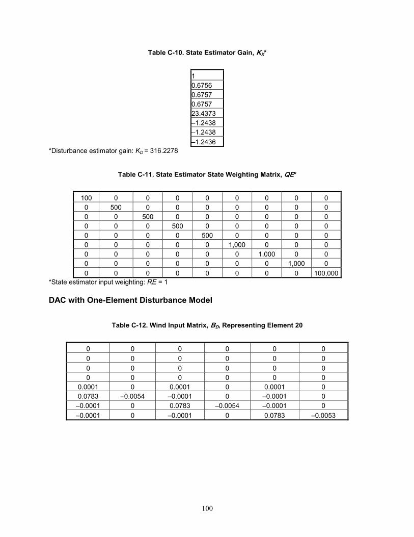
100

Table C-10. State Estimator Gain, KX*

1 0.6756 0.6757 0.6757 23.4373 –1.2438 –1.2438 –1.2436

*Disturbance estimator gain: KD = 316.2278

Table C-11. State Estimator State Weighting Matrix, QE*

100 0 0 0 0 0 0 0 0 0 500 0 0 0 0 0 0 0 0 0 500 0 0 0 0 0 0 0 0 0 500 0 0 0 0 0 0 0 0 0 500 0 0 0 0 0 0 0 0 0 1,000 0 0 0 0 0 0 0 0 0 1,000 0 0 0 0 0 0 0 0 0 1,000 0 0 0 0 0 0 0 0 0 100,000

*State estimator input weighting: RE = 1 DAC with One-Element Disturbance Model

Table C-12. Wind Input Matrix, BD, Representing Element 20

0 0 0 0 0 0 0 0 0 0 0 0 0 0 0 0 0 0 0 0 0 0 0 0

0.0001 0 0.0001 0 0.0001 0 0.0783 –0.0054 –0.0001 0 –0.0001 0 –0.0001 0 0.0783 –0.0054 –0.0001 0 –0.0001 0 –0.0001 0 0.0783 –0.0053

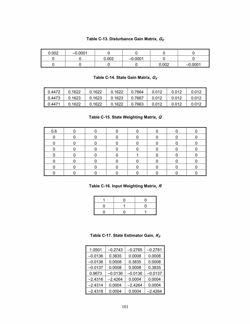
101

Table C-13. Disturbance Gain Matrix, GD

0.002 –0.0001 0 0 0 0

0 0 0.002 –0.0001 0 0 0 0 0 0 0.002 –0.0001

Table C-14. State Gain Matrix, GX

0.4472 0.1622 0.1622 0.1622 0.7664 0.012 0.012 0.012 0.4473 0.1623 0.1623 0.1623 0.7667 0.012 0.012 0.012 0.4471 0.1622 0.1622 0.1622 0.7663 0.012 0.012 0.012

Table C-15. State Weighting Matrix, Q

0.6 0 0 0 0 0 0 0 0 0 0 0 0 0 0 0 0 0 0 0 0 0 0 0 0 0 0 0 0 0 0 0 0 0 0 0 1 0 0 0 0 0 0 0 0 0 0 0 0 0 0 0 0 0 0 0 0 0 0 0 0 0 0 0

Table C-16. Input Weighting Matrix, R

1 0 0 0 1 0 0 0 1

Table C-17. State Estimator Gain, KX

1.0501 –0.2743 –0.2765 –0.2781–0.0136 0.3835 0.0008 0.0008 –0.0136 0.0008 0.3835 0.0008 –0.0137 0.0008 0.0008 0.3835 0.9673 –0.0136 –0.0136 –0.0137–2.4316 –2.4264 0.0004 0.0004 –2.4314 0.0004 –2.4264 0.0004 –2.4318 0.0004 0.0004 –2.4264

102

Table C-18. Disturbance Estimator Gain, KD

1.9113 2.2601 –1.0496 –1.04980.0482 –1.0642 –0.8579 –0.85771.9113 –1.0487 2.2606 –1.04890.0396 –0.8135 –1.0217 –0.81351.9132 –1.0571 –1.0572 2.2522 0.0621 –0.9287 –0.9281 –1.1341

Table C-19. State Estimator State Weighting Matrix, QE

100 0 0 0 0 0 0 0 0 0 0 0 0 0

0 5,000 0 0 0 0 0 0 0 0 0 0 0 0 0 0 5,000 0 0 0 0 0 0 0 0 0 0 0 0 0 0 5,000 0 0 0 0 0 0 0 0 0 0 0 0 0 0 500 0 0 0 0 0 0 0 0 0 0 0 0 0 0 5,000 0 0 0 0 0 0 0 0 0 0 0 0 0 0 5,000 0 0 0 0 0 0 0 0 0 0 0 0 0 0 5,000 0 0 0 0 0 0 0 0 0 0 0 0 0 0 11,000 0 0 0 0 0 0 0 0 0 0 0 0 0 0 10,000 0 0 0 0 0 0 0 0 0 0 0 0 0 0 11,000 0 0 0 0 0 0 0 0 0 0 0 0 0 0 10,000 0 0 0 0 0 0 0 0 0 0 0 0 0 0 11,000 0 0 0 0 0 0 0 0 0 0 0 0 0 0 10,000

Table C-20. State Estimator Input Weighting Matrix, RE

1,000 0 0 0

0 1,000 0 0 0 0 1,000 0 0 0 0 1,000

103

DAC with Hub-Height Uniform Wind Speed and Sinusoidal Vertical Shear Disturbance Model

Table C-21. Wind Input Matrix, BD

0 0 0 0 0 0 0 0 0 0 0 0

0.0511 0 0 0.7735 0.7735 0 0.7736 –0.3868 –0.66990.7735 –0.3868 0.6699

Table C-22. Disturbance Gain Matrix, GD

0.0202 0.0201 0 0 0 0.0202 –0.01 0 –0.0174 0 0.0202 –0.01 0 0.0174 0

Table C-23. State Gain Matrix, GX

0.4472 0.1622 0.1622 0.1622 0.7664 0.012 0.012 0.012 0.4473 0.1623 0.1623 0.1623 0.7667 0.012 0.012 0.012 0.4471 0.1622 0.1622 0.1622 0.7663 0.012 0.012 0.012

Table C-24. State Weighting Matrix, Q

1 0 0 0 0 0 0 0 0 0 0 0 0 0 0 0 0 0 0 0 0 0 0 0 0 0 0 0 0 0 0 0 0 0 0 0 1 0 0 0 0 0 0 0 0 0 0 0 0 0 0 0 0 0 0 0 0 0 0 0 0 0 0 0

104

Table C-25. Input Weighting Matrix, R

1 0 0 0 1 0 0 0 1

Table C-26. State Estimator Gain Matrix, KX

2.8433 6.5008 –1.768 –7.22611.9592 18.2427 0.0307 0.0306 1.9593 0.0307 18.2424 0.0307 1.9592 0.0306 0.0307 18.242924.208 1.9592 1.9593 1.9592

–35.2099 –81.6817 2.4791 2.4786 –35.2079 2.4788 –81.6866 2.4791 –35.2136 2.479 2.4797 –81.6788

Table C-27. State Estimator Disturbance Gain Matrix, KD

194.653 143.8821 143.887 143.8912

0 179.793 –89.9012 –89.9013–0.0055 –88.384 44.1872 44.1853–0.0043 0.0001 –155.708 155.70810.0012 –0.001 76.542 –76.5407

Table C-28. State Estimator State Weighting Matrix, QE

100 0 0 0 0 0 0 0 0 0 0 0 00 1 0 0 0 0 0 0 0 0 0 0 00 0 1 0 0 0 0 0 0 0 0 0 00 0 0 1 0 0 0 0 0 0 0 0 00 0 0 0 500 0 0 0 0 0 0 0 00 0 0 0 0 1,000 0 0 0 0 0 0 00 0 0 0 0 0 1,000 0 0 0 0 0 00 0 0 0 0 0 0 1000 0 0 0 0 00 0 0 0 0 0 0 0 100,000 0 0 0 00 0 0 0 0 0 0 0 0 50,000 0 0 00 0 0 0 0 0 0 0 0 0 0 0 00 0 0 0 0 0 0 0 0 0 0 50,000 00 0 0 0 0 0 0 0 0 0 0 0 0

105

Table C-29. State Estimator Input Weighting Matrix, RE

1 0 0 0 0 1 0 0 0 0 1 0 0 0 0 1

REPORT DOCUMENTATION PAGE

Form Approved OMB NO. 0704-0188

Public reporting burden for this collection of information is estimated to average 1 hour per response, including the time for reviewing instructions, searching existing data sources, gathering and maintaining the data needed, and completing and reviewing the collection of information. Send comments regarding this burden estimate or any other aspect of this collection of information, including suggestions for reducing this burden, to Washington Headquarters Services, Directorate for Information Operations and Reports, 1215 Jefferson Davis Highway, Suite 1204, Arlington, VA 22202-4302, and to the Office of Management and Budget, Paperwork Reduction Project (0704-0188), Washington, DC 20503. 1. AGENCY USE ONLY (Leave blank)

2. REPORT DATE

December 2003

3. REPORT TYPE AND DATES COVERED

Technical Report

4. TITLE AND SUBTITLE Mitigation of Wind Turbine/Vortex Interaction Using Disturbance Accommodating Control

6. AUTHOR(S)

M. Maureen Hand

5. FUNDING NUMBERS

WER3-1940

7. PERFORMING ORGANIZATION NAME(S) AND ADDRESS(ES)

National Renewable Energy Laboratory 1617 Cole Blvd.

Golden, CO 80401-3393

8. PERFORMING ORGANIZATION

REPORT NUMBER NREL/TP-500-35172

9. SPONSORING/MONITORING AGENCY NAME(S) AND ADDRESS(ES)

10. SPONSORING/MONITORING

AGENCY REPORT NUMBER

11. SUPPLEMENTARY NOTES

12a. DISTRIBUTION/AVAILABILITY STATEMENT

National Technical Information Service U.S. Department of Commerce 5285 Port Royal Road

Springfield, VA 22161

12b. DISTRIBUTION CODE

13. ABSTRACT (Maximum 200 words) Complete Descriptive Abstract: Wind turbines, a competitive source of emission-free electricity, are being designed with diameters and hub heights approaching 100 m, to further reduce the cost of the energy they produce. At this height above the ground, the wind turbine is exposed to atmospheric phenomena such as low-level jets, gravity waves, and Kelvin-Helmholtz instabilities, which are not currently modeled in wind turbine design codes. These atmospheric phenomena can generate coherent turbulence that causes high cyclic loads on wind turbine blades. These fluctuating loads lead to fatigue damage accumulation and blade lifetime reduction. Advanced control was used to mitigate vortex-induced blade cyclic loading. A full-state feedback controller that incorporates more detailed vortex inputs achieved significantly greater blade load reduction. Blade loads attributed to vortex passage, then, can be reduced through advanced control, and further reductions appear feasible.

15. NUMBER OF PAGES

14. SUBJECT TERMS

Wind turbine; wind turbine blade; low-level jets; cyclic loading.

16. PRICE CODE

17. SECURITY CLASSIFICATION

OF REPORT Unclassified

18. SECURITY CLASSIFICATION

OF THIS PAGE Unclassified

19. SECURITY CLASSIFICATION

OF ABSTRACT Unclassified

20. LIMITATION OF ABSTRACT

UL

NSN 7540-01-280-5500 Standard Form 298 (Rev. 2-89) Prescribed by ANSI Std. Z39-18 298-102