mixed models in r using the lme4 package part 5...

Mixed models in R using the lme4 packagePart 5: Generalized linear mixed models

Douglas Bates

8th International Amsterdam Conferenceon Multilevel Analysis

<[email protected]>

2011-03-16

Douglas Bates (Multilevel Conf.) GLMM 2011-03-16 1 / 40

Outline

1 Generalized Linear Mixed Models

2 Specific distributions and links

3 Data description and initial exploration

4 Model building

5 Conclusions from the example

6 Summary


Generalized Linear Mixed Models

When using linear mixed models (LMMs) we assume that theresponse being modeled is on a continuous scale.

Sometimes we can bend this assumption a bit if the response is anordinal response with a moderate to large number of levels. Forexample, the Scottish secondary school test results in the mlmRev

package are integer values on the scale of 1 to 10 but we analyzethem on a continuous scale.

However, an LMM is not suitable for modeling a binary response, anordinal response with few levels or a response that represents a count.For these we use generalized linear mixed models (GLMMs).

To describe GLMMs we return to the representation of the responseas an n-dimensional, vector-valued, random variable, Y , and therandom effects as a q-dimensional, vector-valued, random variable, B.


Parts of LMMs carried over to GLMMs

Random variablesY the response variableB the (possibly correlated) random effectsU the orthogonal random effects, such that B = ΛθU

Parametersβ - fixed-effects coefficientsσ - the common scale parameter (not always used)θ - parameters that determine Var(B) = σ2ΛθΛ

Tθ

Some matricesX the n × p model matrix for βZ the n × q model matrix for bP fill-reducing q × q permutation (from Z )Λθ relative covariance factor, s.t. Var(B) = σ2ΛθΛ

Tθ


The conditional distribution, Y |U

For GLMMs, the marginal distribution, B ∼ N (0,Σθ) is the same asin LMMs except that σ2 is omitted. We define U ∼ N (0, I q) suchthat B = ΛθU .

For GLMMs we retain some of the properties of the conditionaldistribution for a LMM

(Y |U = u) ∼ N(µY|U , σ

2I)

where µY|U (u) = Xβ + ZΛθu

SpecificallyI The conditional distribution, Y |U = u , depends on u only through the

conditional mean, µY|U (u).I Elements of Y are conditionally independent. That is, the distribution,

Y |U = u , is completely specified by the univariate, conditionaldistributions, Yi |U , i = 1, . . . ,n.

I These univariate, conditional distributions all have the same form.They differ only in their means.

GLMMs differ from LMMs in the form of the univariate, conditionaldistributions and in how µY|U (u) depends on u .


Some choices of univariate conditional distributions

Typical choices of univariate conditional distributions are:I The Bernoulli distribution for binary (0/1) data, which has probability

mass function

p(y |µ) = µy(1− µ)1−y , 0 < µ < 1, y = 0, 1

I Several independent binary responses can be represented as a binomialresponse, but only if all the Bernoulli distributions have the same mean.

I The Poisson distribution for count (0, 1, . . . ) data, which hasprobability mass function

p(y |µ) = e−µµy

y !, 0 < µ, y = 0, 1, 2, . . .

All of these distributions are completely specified by the conditionalmean. This is different from the conditional normal (or Gaussian)distribution, which also requires the common scale parameter, σ.


The link function, g

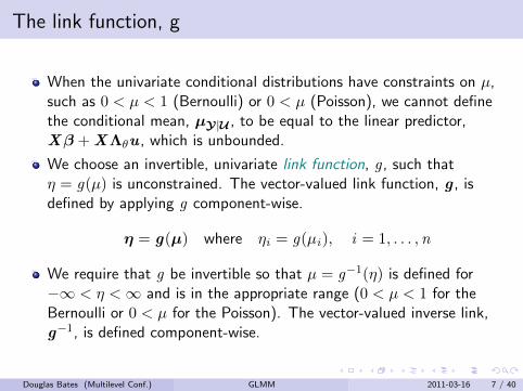
When the univariate conditional distributions have constraints on µ,such as 0 < µ < 1 (Bernoulli) or 0 < µ (Poisson), we cannot definethe conditional mean, µY|U , to be equal to the linear predictor,Xβ +XΛθu , which is unbounded.

We choose an invertible, univariate link function, g , such thatη = g(µ) is unconstrained. The vector-valued link function, g , isdefined by applying g component-wise.

η = g(µ) where ηi = g(µi), i = 1, . . . ,n

We require that g be invertible so that µ = g−1(η) is defined for−∞ < η <∞ and is in the appropriate range (0 < µ < 1 for theBernoulli or 0 < µ for the Poisson). The vector-valued inverse link,g−1, is defined component-wise.


“Canonical” link functions

There are many choices of invertible scalar link functions, g , that wecould use for a given set of constraints.

For the Bernoulli and Poisson distributions, however, one link functionarises naturally from the definition of the probability mass function.(The same is true for a few other, related but less frequently used,distributions, such as the gamma distribution.)

To derive the canonical link, we consider the logarithm of theprobability mass function (or, for continuous distributions, theprobability density function).

For distributions in this “exponential” family, the logarithm of theprobability mass or density can be written as a sum of terms, some ofwhich depend on the response, y , only and some of which depend onthe mean, µ, only. However, only one term depends on both y and µ,and this term has the form y · g(µ), where g is the canonical link.


The canonical link for the Bernoulli distribution

The logarithm of the probability mass function is

log(p(y |µ)) = log(1− µ) + y log

(µ

1− µ

), 0 < µ < 1, y = 0, 1.

Thus, the canonical link function is the logit link

η = g(µ) = log

(µ

1− µ

).

Because µ = P [Y = 1], the quantity µ/(1− µ) is the odds ratio (inthe range (0,∞)) and g is the logarithm of the odds ratio, sometimescalled “log odds”.

The inverse link is

µ = g−1(η) =eη

1 + eη=

1

1 + e−η


Plot of canonical link for the Bernoulli distribution

µ

η=

log(

µ

1−

µ)

−5

0

5

0.0 0.2 0.4 0.6 0.8 1.0


Plot of inverse canonical link for the Bernoulli distribution

η

µ=

1

1+

exp(

−η)

0.0

0.2

0.4

0.6

0.8

1.0

−5 0 5


The canonical link for the Poisson distribution

The logarithm of the probability mass is

log(p(y |µ)) = log(y !)− µ+ y log(µ)

Thus, the canonical link function for the Poisson is the log link

η = g(µ) = log(µ)

The inverse link isµ = g−1(η) = eη


The canonical link related to the variance

For the canonical link function, the derivative of its inverse is thevariance of the response.

For the Bernoulli, the canonical link is the logit and the inverse link isµ = g−1(η) = 1/(1 + e−η). Then

dµ

dη=

e−η

(1 + e−η)2=

1

1 + e−ηe−η

1 + e−η= µ(1− µ) = Var(Y)

For the Poisson, the canonical link is the log and the inverse link isµ = g−1(η) = eη. Then

dµ

dη= eη = µ = Var(Y)


The unscaled conditional density of U |Y = y

As in LMMs we evaluate the likelihood of the parameters, given thedata, as

L(θ,β|y) =∫Rq

[Y |U ](y |u) [U ](u) du ,

The product [Y |U ](y |u)[U ](u) is the unscaled (or unnormalized)density of the conditional distribution U |Y .

The density [U ](u) is a spherical Gaussian density 1(2π)q/2

e−‖u‖2/2.

The expression [Y |U ](y |u) is the value of a probability mass functionor a probability density function, depending on whether Yi |U isdiscrete or continuous.

The linear predictor is g(µY|U ) = η = Xβ + ZΛθu . Alternatively,we can write the conditional mean of Y , given U , as

µY|U (u) = g−1 (Xβ + ZΛθu)


The conditional mode of U |Y = y

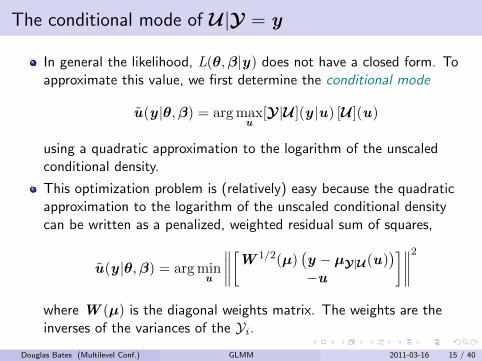
In general the likelihood, L(θ,β|y) does not have a closed form. Toapproximate this value, we first determine the conditional mode

u(y |θ,β) = argmaxu

[Y |U ](y |u) [U ](u)

using a quadratic approximation to the logarithm of the unscaledconditional density.

This optimization problem is (relatively) easy because the quadraticapproximation to the logarithm of the unscaled conditional densitycan be written as a penalized, weighted residual sum of squares,

u(y |θ,β) = argminu

∥∥∥∥[W 1/2(µ)(y − µY|U (u)

)−u

]∥∥∥∥2where W (µ) is the diagonal weights matrix. The weights are theinverses of the variances of the Yi .


The PIRLS algorithm

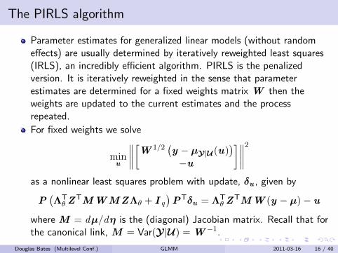
Parameter estimates for generalized linear models (without randomeffects) are usually determined by iteratively reweighted least squares(IRLS), an incredibly efficient algorithm. PIRLS is the penalizedversion. It is iteratively reweighted in the sense that parameterestimates are determined for a fixed weights matrix W then theweights are updated to the current estimates and the processrepeated.

For fixed weights we solve

minu

∥∥∥∥[W 1/2(y − µY|U (u)

)−u

]∥∥∥∥2as a nonlinear least squares problem with update, δu , given by

P(ΛTθ Z

TMWMZΛθ + I q

)PTδu = ΛT

θ ZTMW (y − µ)− u

where M = dµ/dη is the (diagonal) Jacobian matrix. Recall that forthe canonical link, M = Var(Y |U) = W −1.


The Laplace approximation to the deviance

At convergence, the sparse Cholesky factor, L, used to evaluate theupdate is

LLT = P(ΛTθ Z

TMWMZΛθ + I q

)PT

orLLT = P

(ΛTθ Z

TMZΛθ + I q

)PT

if we are using the canonical link.

The integrand of the likelihood is approximately a constant times thedensity of the N (u ,LLT) distribution.

On the deviance scale (negative twice the log-likelihood) thiscorresponds to

d(β,θ|y) = dg(y ,µ(u)) + ‖u‖2 + log(|L|2)

where dg(y ,µ(u)) is the GLM deviance for y and µ.


Modifications to the algorithm

Notice that this deviance depends on the fixed-effects parameters, β,as well as the variance-component parameters, θ. This is becauselog(|L|2) depends on µY|U and, hence, on β. For LMMs log(|L|2)depends only on θ.

In practice we begin by optimizing w.r.t. u and β simultaneously,evaluating the Laplace approximation and optimizing this w.r.t. θ.Then we use a “pure” Laplace approximation which is optimized w.r.t.both β and θ.

The second stage can be suppressed with the optional argument nAGQ= 0. Another argument verbose = 2 shows the two stages explicitly

Another approach is adaptive Gauss-Hermite quadrature (AGQ). Thishas a similar structure to the Laplace approximation but is based onmore evaluations of the unscaled conditional density near theconditional modes. It is only appropriate for models in which therandom effects are associated with only one grouping factor


Contraception data

One of the data sets in the "mlmRev" package, derived from data filesavailable on the multilevel modelling web site, is from a fertilitysurvey of women in Bangladesh.

One of the (binary) responses recorded is whether or not the womancurrently uses artificial contraception.

Covariates included the woman’s age (on a centered scale), thenumber of live children she had, whether she lived in an urban or ruralsetting, and the district in which she lived.

Instead of plotting such data as points, we use the 0/1 response togenerate scatterplot smoother curves versus age for the differentgroups.


Contraception use versus age by urban and livch

Centered age

Pro

port

ion

0.0

0.2

0.4

0.6

0.8

1.0

−10 0 10 20

N

−10 0 10 20

Y

0 1 2 3+


Comments on the data plot

These observational data are unbalanced (some districts have only 2observations, some have nearly 120). They are not longitudinal (no“time” variable).

Binary responses have low per-observation information content(exactly one bit per observation). Districts with few observations willnot contribute strongly to estimates of random effects.

Within-district plots will be too imprecise so we only examine theglobal effects in plots.

The comparisons on the multilevel modelling site are for fits of amodel that is linear in age, which is clearly inappropriate.

The form of the curves suggests at least a quadratic in age.

The urban versus rural differences may be additive.

It appears that the livch factor could be dichotomized into“0”versus“1 or more”.


Preliminary model using Laplacian approximation

Generalized linear mixed model fit by maximum likelihood [’merMod’]

Family: binomial

Formula: use ~ age + I(age^2) + urban + livch + (1 | district)

Data: Contraception

AIC BIC logLik deviance

2388.785 2433.323 -1186.392 2372.785

Random effects:

Groups Name Variance Std.Dev.

district (Intercept) 0.2253 0.4747

Number of obs: 1934, groups: district, 60

Fixed effects:

Estimate Std. Error z value

(Intercept) -1.0152756 0.1739721 -5.836

age 0.0035135 0.0092106 0.381

I(age^2) -0.0044867 0.0007228 -6.207

urbanY 0.6844018 0.1196840 5.718

livch1 0.8018807 0.1618666 4.954

livch2 0.9010171 0.1847709 4.876

livch3+ 0.8994111 0.1854007 4.851


Comments on the model fit

This model was fit using the Laplacian approximation to the deviance.

There is a highly significant quadratic term in age.

The linear term in age is not significant but we retain it because theage scale has been centered at an arbitrary value (which,unfortunately, is not provided with the data).

The urban factor is highly significant (as indicated by the plot).

Levels of livch greater than 0 are significantly different from 0 butmay not be different from each other.


Reduced model with dichotomized livch


Family: binomial

Formula: use ~ age + I(age^2) + urban + ch + (1 | district)

Data: Contraception


2385.241 2418.645 -1186.621 2373.241

Random effects:




Fixed effects:


(Intercept) -0.987377 0.167529 -5.894

age 0.006170 0.007826 0.788

I(age^2) -0.004558 0.000714 -6.384

urbanY 0.680226 0.119476 5.693

chY 0.846208 0.147027 5.755


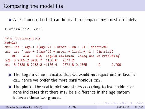
Comparing the model fits

A likelihood ratio test can be used to compare these nested models.

> anova(cm2 , cm1)

Data: Contraception

Models:

cm2: use ~ age + I(age^2) + urban + ch + (1 | district)

cm1: use ~ age + I(age^2) + urban + livch + (1 | district)

Df AIC BIC logLik deviance Chisq Chi Df Pr(>Chisq)

cm2 6 2385.2 2418.7 -1186.6 2373.2

cm1 8 2388.8 2433.3 -1186.4 2372.8 0.4565 2 0.796

The large p-value indicates that we would not reject cm2 in favor ofcm1 hence we prefer the more parsimonious cm2.

The plot of the scatterplot smoothers according to live children ornone indicates that there may be a difference in the age patternbetween these two groups.


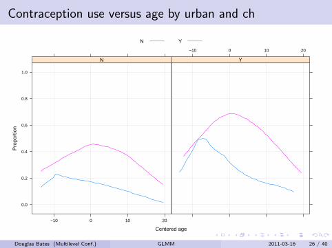
Contraception use versus age by urban and ch

Centered age

Pro

port

ion

0.0

0.2

0.4

0.6

0.8

1.0

−10 0 10 20

N

−10 0 10 20

Y

N Y


Allowing age pattern to vary with ch


Family: binomial

Formula: use ~ age * ch + I(age^2) + urban + (1 | district)

Data: Contraception


2379.181 2418.153 -1182.591 2365.181

Random effects:




Fixed effects:


(Intercept) -1.3230260 0.2144340 -6.170

age -0.0472742 0.0218378 -2.165

chY 1.2105520 0.2069791 5.849

I(age^2) -0.0057574 0.0008358 -6.889

urbanY 0.7139915 0.1202574 5.937

age:chY 0.0683363 0.0254331 2.687


Prediction intervals on the random effectsS

tand

ard

norm

al q

uant

iles

−2

−1

0

1

2

−1.5 −1.0 −0.5 0.0 0.5 1.0

●

●

●

●

●

●●●

●●

●●●

●●

●●●●●

●●●●●●● ●●

●● ●●●●●●

●●

●●●

●●●●●

●●

●●

●●

●●

●

●

●

●

●


Extending the random effects

We may want to consider allowing a random effect for urban/rural bydistrict. This is complicated by the fact the many districts only haverural women in the study

district

urban 1 2 3 4 5 6 7 8 9 10 11 12 13 14 15 16

N 54 20 0 19 37 58 18 35 20 13 21 23 16 17 14 18

Y 63 0 2 11 2 7 0 2 3 0 0 6 8 101 8 2

district

urban 17 18 19 20 21 22 23 24 25 26 27 28 29 30 31 32

N 24 33 22 15 10 20 15 14 49 13 39 45 25 45 27 24


Including a random effect for urban by district


Family: binomial

Formula: use ~ age * ch + I(age^2) + urban + (urban | district)

Data: Contraception


2371.530 2421.636 -1176.765 2353.530

Random effects:

Groups Name Variance Std.Dev. Corr


urbanY 0.5261 0.7253 -0.793


Fixed effects:


(Intercept) -1.3441450 0.2227632 -6.034

age -0.0461824 0.0219444 -2.105

chY 1.2116385 0.2082354 5.819

I(age^2) -0.0056514 0.0008431 -6.703

urbanY 0.7901052 0.1600452 4.937

age:chY 0.0664711 0.0255671 2.600

Correlation of Fixed Effects:

(Intr) age chY I(g^2) urbanY

age 0.696

chY -0.855 -0.792

I(age^2) -0.091 0.301 -0.097

urbanY -0.370 -0.061 0.088 -0.018

age:chY -0.575 -0.930 0.676 -0.496 0.055


Significance of the additional random effect

> anova(cm4 ,cm3)

Data: Contraception

Models:

cm3: use ~ age * ch + I(age^2) + urban + (1 | district)

cm4: use ~ age * ch + I(age^2) + urban + (urban | district)


cm3 7 2379.2 2418.2 -1182.6 2365.2

cm4 9 2371.5 2421.6 -1176.8 2353.5 11.651 2 0.002951

The additional random effect is highly significant in this test.

Most of the prediction intervals still overlap zero.

A scatterplot of the random effects shows several random effectsvectors falling along a straight line. These are the districts with allrural women or all urban women.


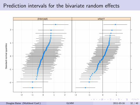
Prediction intervals for the bivariate random effectsS

tand

ard

norm

al q

uant

iles

−2

−1

0

1

2

−2 −1 0 1 2

●

●

●

●

●●●●●●●●●●●●●●●●●●●●●●

●●●●●●●●●●●●●

●●●●●●●

●●

●●●●●●●●

●

●

●

●

(Intercept)

−2 −1 0 1

●

●

●

●

●●

●●

●●●●●●●●●●

●●●● ●●

●●●●●●●

●●●●●●●●●●●●●●●●

●●●●●●●●●

●

●

●

●

urbanY


Scatter plot of the BLUPs

urbanY

(Int

erce

pt)

−1.0

−0.5

0.0

0.5

1.0

−1.0 −0.5 0.0 0.5 1.0

●

●●

●

●

●

●

●

●

●

●

●

●

●

●

●

●

●●

●

●

●

●

●

●

●

●

● ●

●

●

●

●

●

●

●

●

●

●

●

●

● ●

●

●

●

●

●

●

●●

●

●●

●

●

●

●●●


Nested simple, scalar random effects versus vector-valued


Family: binomial

Formula: use ~ age * ch + I(age^2) + urban + (1 | urban:district) + (1 | district)

Data: Contraception


2370.464 2415.003 -1177.232 2354.464

Random effects:


urban:district (Intercept) 0.30987 0.5567


Number of obs: 1934, groups: urban:district, 102; district, 60

Fixed effects:


(Intercept) -1.3406181 0.2210382 -6.065

age -0.0461495 0.0220190 -2.096

chY 1.2129371 0.2089635 5.805

I(age^2) -0.0056309 0.0008437 -6.674

urbanY 0.7833789 0.1691559 4.631

age:chY 0.0664924 0.0256365 2.594


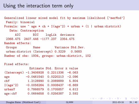
Using the interaction term only


Family: binomial

Formula: use ~ age * ch + I(age^2) + urban + (1 | urban:district)

Data: Contraception


2368.475 2407.446 -1177.237 2354.475

Random effects:


urban:district (Intercept) 0.3229 0.5683

Number of obs: 1934, groups: urban:district, 102

Fixed effects:


(Intercept) -1.3406928 0.2211336 -6.063

age -0.0461540 0.0220213 -2.096

chY 1.2128990 0.2089889 5.804

I(age^2) -0.0056264 0.0008437 -6.669

urbanY 0.7866579 0.1705857 4.612

age:chY 0.0664658 0.0256387 2.592


Comparing models with random effects for interactions

> anova(cm6 ,cm5 ,cm4)

Data: Contraception

Models:

cm6: use ~ age * ch + I(age^2) + urban + (1 | urban:district)

cm5: use ~ age * ch + I(age^2) + urban + (1 | urban:district) + (1 |

cm5: district)

cm4: use ~ age * ch + I(age^2) + urban + (urban | district)


cm6 7 2368.5 2407.4 -1177.2 2354.5

cm5 8 2370.5 2415.0 -1177.2 2354.5 0.0107 1 0.9177

cm4 9 2371.5 2421.6 -1176.8 2353.5 0.9338 1 0.3339

The random effects seem to best be represented by a separaterandom effect for urban and for rural women in each district.

The districts with only urban women in the survey or with only ruralwomen in the survey are naturally represented in this model.


Showing the optimization stages

> cm6 <- glmer(use ~ age*ch + I(age^2) + urban + (1| urban:district),

+ Contraception , binomial , verbose =2L)

npt = 3 , n = 1

rhobeg = 0.2 , rhoend = 2e-07

0.020: 5: 2354.74;0.600000

0.0020: 8: 2354.59;0.572147

0.00020: 11: 2354.59;0.567988

2.0e-05: 13: 2354.59;0.567275

2.0e-06: 14: 2354.59;0.567275

2.0e-07: 15: 2354.59;0.567273

At return

18: 2354.5894: 0.567273

npt = 9 , n = 7

rhobeg = 2e-04 , rhoend = 2e-07

2.0e-05: 11: 2354.54;0.567273 -1.30421 -0.0446451 1.18092 -0.00567546 0.764306 0.0646009

2.0e-06: 24: 2354.52;0.567257 -1.30425 -0.0444421 1.18090 -0.00561934 0.764246 0.0647203

2.0e-07: 300: 2354.51;0.567979 -1.30454 -0.0436418 1.18099 -0.00561732 0.765138 0.0639954

At return

3743: 2354.4746: 0.568279 -1.34069 -0.0461540 1.21290 -0.00562640 0.786658 0.0664658


Conclusions from the example

Again, carefully plotting the data is enormously helpful in formulatingthe model.

Observational data tend to be unbalanced and have many morecovariates than data from a designed experiment. Formulating amodel is typically more difficult than in a designed experiment.

A generalized linear model is fit with the function glmer() whichrequires a family argument. Typical values are binomial or poisson

Profiling is not provided for GLMMs at present but will be added.

We use likelihood-ratio tests and z-tests in the model building.


A word about overdispersion

In many application areas using “pseudo” distribution families, such asquasibinomial and quasipoisson, is a popular and well-acceptedtechnique for accomodating variability that is apparently larger thanwould be expected from a binomial or a Poisson distribution.

This amounts to adding an extra parameter, like σ, the common scaleparameter in a LMM, to the distribution of the response.

It is possible to form an estimate of such a quantity during the IRLSalgorithm but it is an artificial construct. There is no probabilitydistribution with such a parameter.

I find it difficult to define maximum likelihood estimates without aprobability model. It is not clear how this “distribution which is not adistribution” could be incorporated into a GLMM. This, of course,does not stop people from doing it but I don’t know what theestimates from such a model would mean.


Summary

GLMMs allow for the conditional distribution, Y|B = b, to be otherthan a Gaussian. A Bernoulli (or, more generally, a binomial)distribution is used to model binary or binomial responses. A Poissondistribution is used to model responses that are counts.

The conditional mean depends upon the linear predictor, Xβ + Zb,through the inverse link function, g−1.

The conditional mode of the random effects, given the observed data,y , is determined through penalized iteratively reweighted leastsquares (PIRLS).

We optimize the Laplace approximation at the conditional mode todetermine the mle’s of the parameters. In some simple cases, a moreaccurate approximation, adaptive Gauss-Hermite quadrature (AGQ),can be used instead, at the expense of greater computationalcomplexity.


mixed models in r using the lme4 package part 5...

Documents