mixsim 2.1 tutorial -...

MIXSIM 2.1 Tutorial

November 2006

c© Fluent Inc. November 8, 2006 1

kcg

Rectangle

Copyright c© 2006 by Fluent Inc.All Rights Reserved. No part of this document may be reproduced or otherwise used in

any form without express written permission from Fluent Inc.

Airpak, FIDAP, FLUENT, FLUENT for CATIA V5, FloWizard, GAMBIT, Icemax, Icepak,Icepro, Icewave, Icechip, MixSim, and POLYFLOW are registered trademarks of FluentInc. All other products or name brands are trademarks of their respective holders.

CHEMKIN is a registered trademark of Reaction Design Inc.

Portions of this program include material copyrighted by PathScale Corporation2003-2004.

Fluent Inc.Centerra Resource Park

10 Cavendish CourtLebanon, NH 03766

2 c© Fluent Inc. November 8, 2006

kcg

Rectangle

Tutorial: Cylindrical Vessel with a Pitched Blade Impeller

and Flat Baffles

Introduction

The purpose of this tutorial is to introduce to you, the MixSim 2.1 user interface and thetypical problem-solving procedure. It illustrates the setup and solution of a simple mixerconfiguration consisting of a cylindrical vessel with a pitched blade impeller and four baffles.This configuration is commonly used in process industries for mixing and related operations.

This tutorial demonstrates how to do the following:

• Create a new model.

• Specify the fluid and its relevant properties.

• Define the tank, baffles, shaft, and impeller geometry.

• Generate the grid.

• Perform the calculation.

• Postprocess the results.

Prerequisites

This tutorial assumes that you have read Chapters 3 and 4 of the MixSim User’s Guide andare familiar with the basic user interface elements.

Problem Description

The configuration considered in this tutorial is shown in Figure 1. The cylindrical tank,with an ASME 10% tank bottom shape, has a diameter of 1.0 m, a liquid level height of1.0 m, and an open top. This means that the top shape of the tank is not specified, becausethe liquid level remains in the cylindrical part of the tank.

The tank contains a top mounted, centrally located shaft, a pitched blade axial flow impellermounted to it, and four flat baffles. The fluid in the tank is water. The liquid flow field issolved and displayed during postprocessing.


Cylindrical Vessel with a Pitched Blade Impeller and Flat Baffles

Figure 1: Problem Schematic

Step 1: Starting a New Session

1. Start MixSim.

2. Create a new model.

File −→New Model

The Model Management panel and a graphics display window will open. The modeldetails and geometry are defined in the Model Management panel. This panel containsan Object Tree, Graphics Display, and some text-entry boxes. The graphics displaywindow shows three views of the geometry: front view, top view, and a view that youcan manipulate. Arrange these windows on your screen so that both are visible.



3. Specify an appropriate title and a brief description in the Title and Description fields,respectively.

The text entered in the Title and Description fields appears only in the the ModelManagement panel (here) and at the top of the generated HTML report.

4. Enter cyl-pitched-blade for File Name.

This file name will be used as a prefix for all files that are automatically created byMixSim, (mesh and data files).



5. Retain the selection of MRF in the Analysis Type drop-down list.

6. Click Apply to save your inputs.

You need to click Apply to save your inputs after modifying any entry in the ModelManagement panel.

Step 2: Fluid Properties

You need not visit the Continuum panel if you plan to run the simulation with the defaultsettings. You can directly set the fluid material. Here, we introduce to you the interface ele-ments that can be used to choose different settings for the turbulance model and/ot materialproperties.

1. Select Continuum in the Object Tree.

The Model Management panel will show a set of buttons for handling materials andrelated models.

2. Click the Viscous Model button to open the Viscous Model panel.

You can specify either laminar or turbulent flow in the Viscous Model panel. You canselect the turbulence model to be used. The default Realizable k-epsilon model is usedin this example.

(a) Retain the default selection of k-epsilon (2 eqn) in the Model list and Realizablein the k-epsilon Model list, respectively.

(b) Click OK to close the Viscous Model panel.

(c) Click Apply in the Model Management panel to save the settings.



Two more buttons (Edit Materials and Copy Material) are provided in the Continuumobject panel. They allow you to copy one or more materials from a database into theMixSim session and edit (modify) them. For more information on using the Mate-rials panel and adding new materials to the database, refer to Section 6.3: PhysicalProperties in the MixSim User’s Guide.

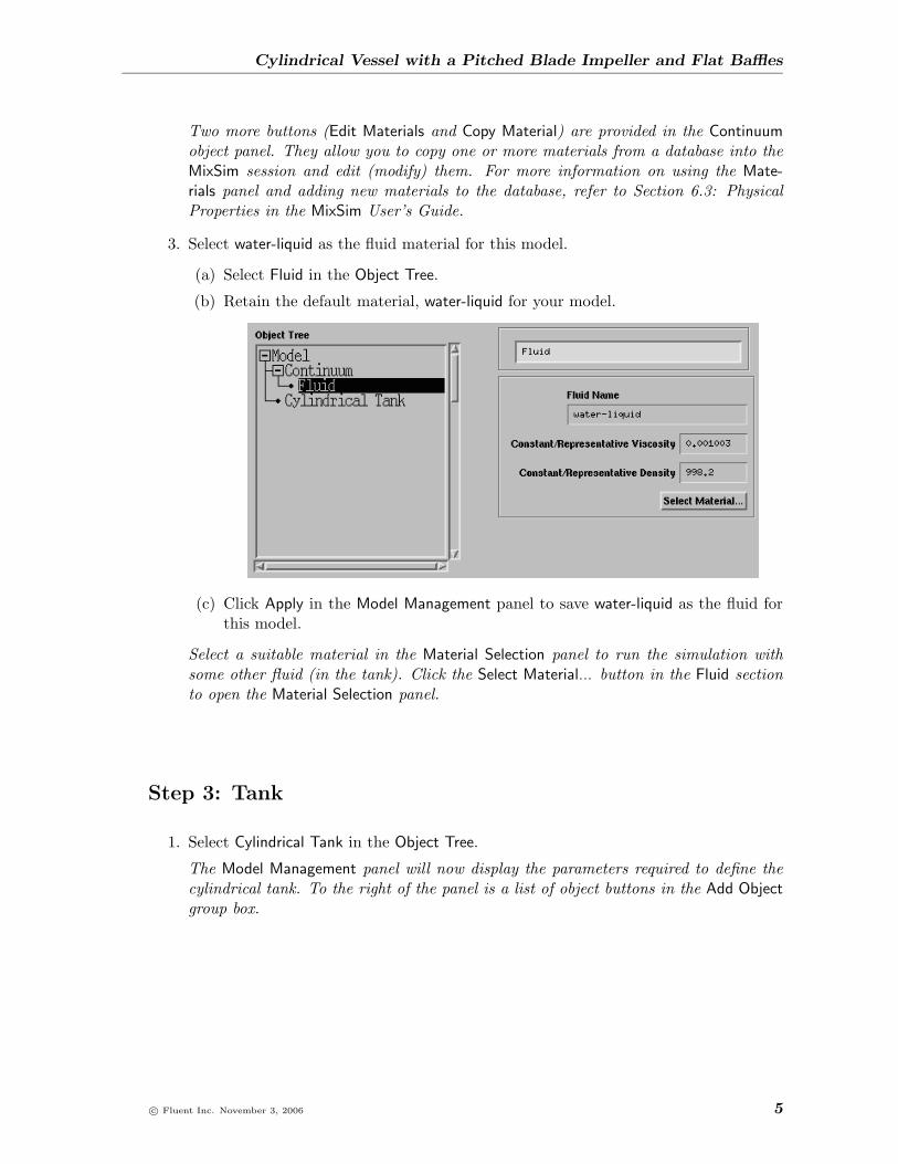
3. Select water-liquid as the fluid material for this model.

(a) Select Fluid in the Object Tree.

(b) Retain the default material, water-liquid for your model.

(c) Click Apply in the Model Management panel to save water-liquid as the fluid forthis model.

Select a suitable material in the Material Selection panel to run the simulation withsome other fluid (in the tank). Click the Select Material... button in the Fluid sectionto open the Material Selection panel.

Step 3: Tank

1. Select Cylindrical Tank in the Object Tree.

The Model Management panel will now display the parameters required to define thecylindrical tank. To the right of the panel is a list of object buttons in the Add Objectgroup box.



2. Retain the default values for Diameter, Tank Height, and Liquid Level of the tank.

3. Retain the selection of Open in the Top Style drop-down list.

4. Select ASME (10%) in the Bottom Style drop-down list.

5. Retain other default settings and click Apply.

The graphics display in the Model Management panel and graphics window are updatedto display the tank according to your specifications. You can manipulate the view inthe top right frame of the preview graphics window. You can rotate the image usingthe left mouse button, zoom the image using the right mouse button and center theimage in the window using the middle mouse button.



Figure 2: Cylindrical Tank with ASME 10% Bottom Style

Step 4: Baffles

1. Click Baffle in the Add Object group box.

A Baffle frame with a list of different types of baffles is displayed.

2. Click Flat Baffles in the Baffle frame.

The Model Management panel will now display the parameters for the flat baffles.



3. Retain 0.194 m for Bottom Elevation.

4. Enter 1.1 for Top Elevation.

This will allow the baffles to extend to the top of the tank.

5. Retain the default value of 0.1 m for Width and Distance from Wall.

6. Make sure that the Zero Thickness Baffle option is enabled.

Note: MixSim will neglect the baffle thickness in the simulated geometry and compu-tational grid when the Zero Thickness Baffle option is enabled. This will reducethe number of computational cells and hence, the memory (RAM) and calculationtime for the solution, without significantly affecting the accuracy of the results.

7. Retain the default values for other parameters and click Apply.

The graphics window is updated to display the tank with the baffles (Figure 3).



Figure 3: Tank with Flat Baffles

Step 5: Shaft

1. Click Cylindrical Tank in the Object Tree.

To add another “child” object to the vessel, you must go back to the parent object.

2. Click Shaft in the Add Object group box.

A Shaft frame with a list of different types of shafts will be displayed.



3. Click Top Shaft in the Shaft frame.

The Model Management panel will now display the parameters required to define thetop shaft.

4. Enter 150 rpm for Speed.

5. Enter 0.3 m for Shaft Tip Elevation and click Apply.

The graphics window is updated to display the tank with the baffles and the shaft.



Figure 4: Tank with Baffles and Shaft

Step 6: Impeller

1. Click Generic Impellers in the Add Object group box.

A Generic Impellers frame with a list of different impeller models will be displayed.

2. Click the Pitched Blade button in the Generic Impellers frame.

The Model Management panel will now display the parameters required to define thePitched Blade impeller.

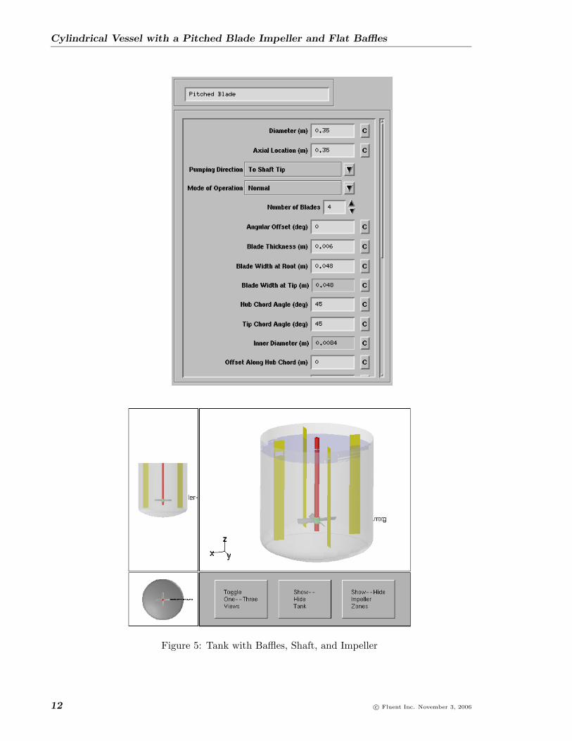
3. Enter 0.35 m for Diameter in order to resize the impeller to suit the tank dimensions.

4. Enter 0.35 m for Axial Location.

5. Retain other default parameters and click Apply. The graphics window is updated todisplay the tank with baffles, shaft, and impeller (Figure 5).

6. Close the Model Management panel.



Figure 5: Tank with Baffles, Shaft, and Impeller



7. Save the MixSim model.

File −→ Write −→MixSim Model...

(a) Retain the suggested file name (cyl-pitched-blade.mxm) and click OK.

The suggested file name in the Write:MixSim Model File field (cyl-pitched-blade.mxm)is automatically generated from the File Name parameter, entered in the Model Man-agement panel at the beginning of the session. This file name is generated only once.If you change the File Name parameter after saving the model once, the suggested filename for Write:MixSim Model File will not change.

Step 7: Grid

1. Generate the grid.

Grid −→Generate Grid...

MixSim uses the GAMBIT process in the background to create the geometry and gen-erate the grid. As the grid is generated, GAMBIT commands appear on the MixSimconsole and a progress bar panel will show the rate of completion of the grid generationprocess.



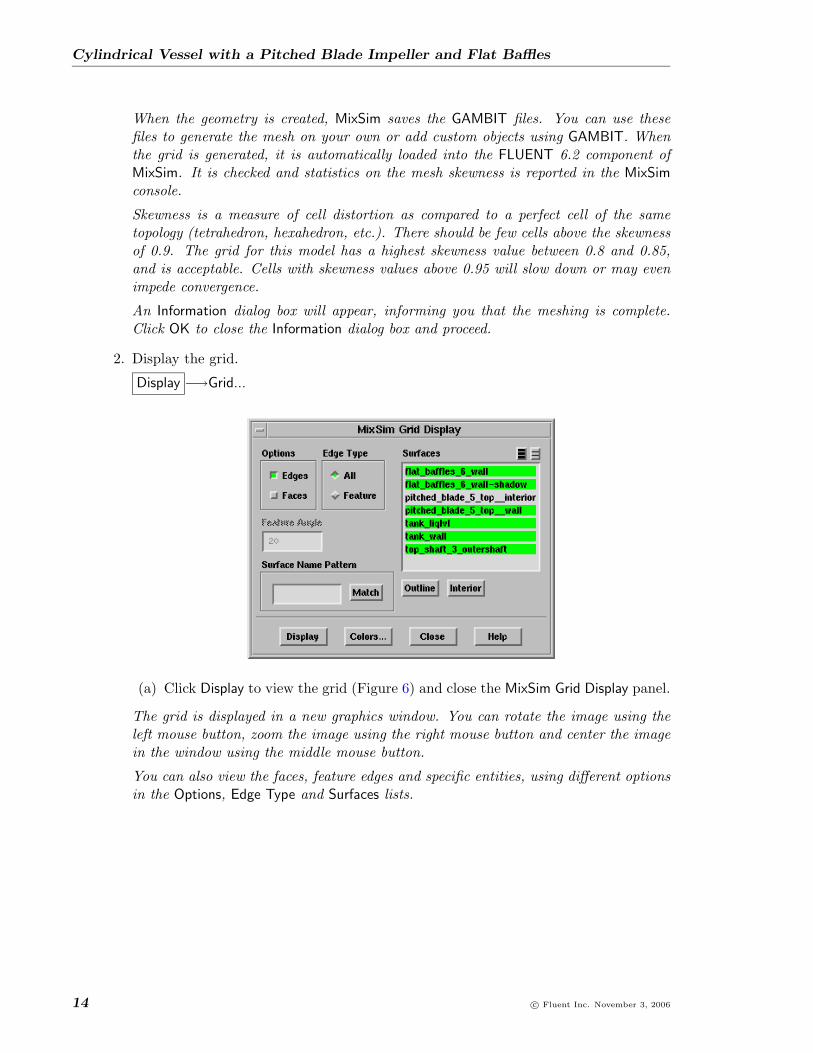
When the geometry is created, MixSim saves the GAMBIT files. You can use thesefiles to generate the mesh on your own or add custom objects using GAMBIT. Whenthe grid is generated, it is automatically loaded into the FLUENT 6.2 component ofMixSim. It is checked and statistics on the mesh skewness is reported in the MixSimconsole.

Skewness is a measure of cell distortion as compared to a perfect cell of the sametopology (tetrahedron, hexahedron, etc.). There should be few cells above the skewnessof 0.9. The grid for this model has a highest skewness value between 0.8 and 0.85,and is acceptable. Cells with skewness values above 0.95 will slow down or may evenimpede convergence.

An Information dialog box will appear, informing you that the meshing is complete.Click OK to close the Information dialog box and proceed.

2. Display the grid.

Display −→Grid...

(a) Click Display to view the grid (Figure 6) and close the MixSim Grid Display panel.

The grid is displayed in a new graphics window. You can rotate the image using theleft mouse button, zoom the image using the right mouse button and center the imagein the window using the middle mouse button.

You can also view the faces, feature edges and specific entities, using different optionsin the Options, Edge Type and Surfaces lists.



Figure 6: Grid Display

Step 8: Solution

1. Start the calculation.

Solve −→Iterate

The default number of iterations is 10.

2. Retain the number of initial iterations.

MixSim sets up and runs the calculation using its FLUENT component. During thecalculation, MixSim will display convergence monitor plots for turbulent kinetic energy(averaged on the free liquid surface), shaft moment (torque), and scaled residuals.



These plots tell you when the solution has finished. When the (scaled) residuals aresmall and some representative quantities do not change (significantly) between itera-tions any more, you may assume that the iterative solution has converged and moreiterations will not improve the result further. The representative quantities are chosenand plotted automatically by MixSim, and are used for the first two monitor plots.

The values of these monitor quantities usually take very large negative or positivevalues during the first few iterations and then rapidly approach a relatively narrowrange close to the final value. Judging the relative change in these values from oneiteration to the next is difficult, because the interesting changes are squeezed verticallyin the plots that still contain much higher initial values. To improve the plot aroundthe final value, you should clear the plot after the first few iterations. For this reason,perform only 10 iterations when you begin the solution.

For the guidelines on setting the number of iterations, see Section 14.2.2 in Chapter14: Performing the Calculation.

3. Click Iterate to start the calculation.

The automatically created plot windows are shown in Figures 7, 8, and 9.

Z

Y

X

Scaled ResidualsMixSim 2.1 (2.1.10)

Iterations1086420

1e+01

1e+00

1e-01

1e-02

epsilonkz-velocityy-velocityx-velocitycontinuityResiduals

Figure 7: Residual Plot



Z

Y

X

Convergence history of Turbulence Kinetic Energy (k) on tank_liqlvlMixSim 2.1 (2.1.10)

Iteration

(m2/s2)Values

Facetof

Sum

1086420

0.5000

0.4000

0.3000

0.2000

0.1000

0.0000

symmonMonitors

Figure 8: Convergence Plot for Turbulent Kinetic Energy

ZYX

Moment Convergence History About Z-AxisMixSim 2.1 (2.1.10)

Iterations

Cm

10987654321

140.0000

120.0000

100.0000

80.0000

60.0000

40.0000

20.0000

0.0000

Figure 9: Moment Convergence History About the Z-axis



4. Click the Reset Monitor Plot Data button in the Iterate panel.

This resets the monitor plots. Otherwise, the automatic scaling of the ordinate axesin the monitor plots will cause the a part of the plot to be vertically compressed sothat no useful information can be seen.

Solve −→Iterate

(a) Click Reset Monitor Plot Data.

5. Reset the number of iterations.

Mixing tank models generally take approximately 5000 iterations to converge. Gener-ally, a mixing simulation is considered to be converged when both, the shaft torque/momentand the turbulence energy monitors flatten out and the residuals are flat and below1 · 10−5. When the residuals fall below 1 · 10−5 and the monitors flatten out, it is notnecessary for the scaled residuals to become constant/flat.

(a) Make sure that the Initialize option is disabled.

(b) Enable the Save Case and Save Data options.

This will make sure that the case and data files are saved in the working directoryat the end of the simulation. Alternatively, you can disable these options and savethe files manually after the iterations have been completed.

(c) Enter 5000 for Iterations and click Iterate.

The residuals and monitor plots at the end of 5000 iterations are shown in Fig-ures 10, 11, and 12.

Completing 5000 iterations may take quite some time. If for a different model,you find that the monitor quantities are constant after fewer (e.g. 3000) itera-tions, click Cancel in the Working dialog box or type <Ctrl-C> in the MixSimconsole to interrupt the solver. Allow some time for the solver to process yourrequest for interruption.

To obtain an accurate solution perform the calculation using higher order discretiza-!tion. To switch to higher order discretization, click the Switch to Higher Accuracybutton in the Iterate panel and continue iterations till the solution appears converged.



Z

Y

X

Scaled ResidualsMixSim 2.1 (2.1.10)

Iterations6000500040003000200010000

1e+00

1e-01

1e-02

1e-03

1e-04

1e-05

1e-06

1e-07

epsilonkz-velocityy-velocityx-velocitycontinuityResiduals

Figure 10: Residual Plot

Z

Y

X

Convergence history of Turbulence Kinetic Energy (k) on tank_liqlvlMixSim 2.1 (2.1.10)

Iteration

(m2/s2)Values

Facetof

Sum

6000500040003000200010000

5.0000

4.5000

4.0000

3.5000

3.0000

2.5000

2.0000

1.5000

1.0000

0.5000

0.0000

symmonMonitors

Figure 11: Convergence Plots for Turbulent Kinetic Energy



ZYX

Moment Convergence History About Z-AxisMixSim 2.1 (2.1.10)

Iterations

Cm

55005000450040003500300025002000150010005000

7.2500

7.0000

6.7500

6.5000

6.2500

6.0000

5.7500

5.5000

5.2500

5.0000

4.7500

Figure 12: Moment Convergence History About the Z-axis

Step 9: Postprocessing

You can use the case and data files provided with this tutorial to proceed with the post-processing for this problem. To do so, start a new MixSim session, load (or read) themodel file (cyl-pitched-blade.mxm) and then load the FLUENT case and data files pro-vided (cyl-pitched-blade.cas and cyl-pitched-blade.dat).

1. Start a new MixSim session.

2. Read the MixSim model file provided with this tutorial.

File −→ Read −→MixSim Model...

Select cyl-pitched-blade.mxm from the Files list and click OK.

3. Read the converged case and data files provided with this tutorial:

File −→ Read −→Case & Data...

Select cyl-pitched-blade.cas from the Files list and click OK.

4. Display velocity vectors that start from the impeller surface.

Display −→Vectors...

(a) Enter 10 for Scale and retain the setting of 0 for Skip.

(b) Select the impeller surface pitched blade 5 top wall from the Surfaces selectionlist.



(c) Retain other default parameters and click Display to plot the vectors (Figure 13).

You can confirm that the impeller is rotating clockwise and pumping down.

Note: You can manipulate the graphics display with the mouse in the same wayas when you displayed the grid.

Figure 13: Vectors of Velocity Magnitude

(d) Modify the vector display.

i. Enable Lights On and Show Tank in the Options group box in the Vectorspanel.



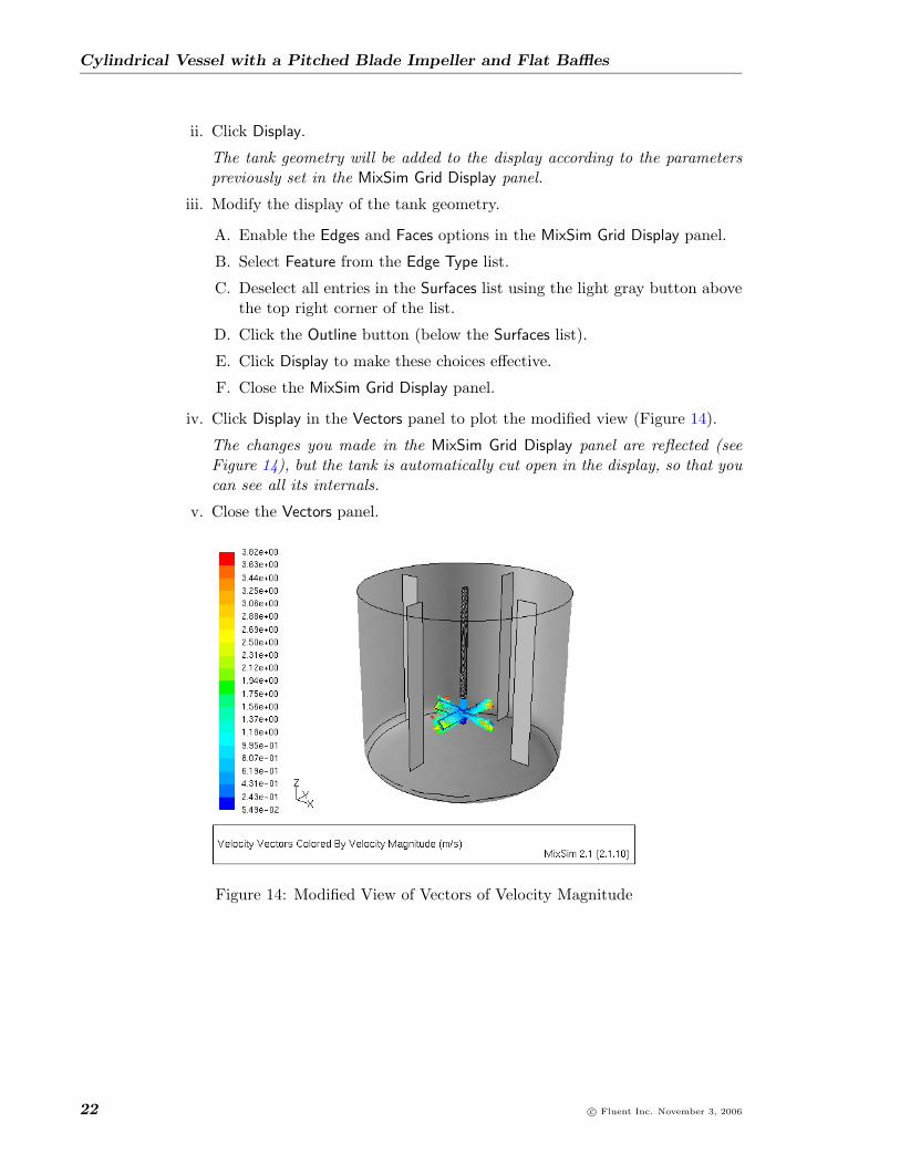
ii. Click Display.

The tank geometry will be added to the display according to the parameterspreviously set in the MixSim Grid Display panel.

iii. Modify the display of the tank geometry.

A. Enable the Edges and Faces options in the MixSim Grid Display panel.

B. Select Feature from the Edge Type list.

C. Deselect all entries in the Surfaces list using the light gray button abovethe top right corner of the list.

D. Click the Outline button (below the Surfaces list).

E. Click Display to make these choices effective.

F. Close the MixSim Grid Display panel.

iv. Click Display in the Vectors panel to plot the modified view (Figure 14).

The changes you made in the MixSim Grid Display panel are reflected (seeFigure 14), but the tank is automatically cut open in the display, so that youcan see all its internals.

v. Close the Vectors panel.

Figure 14: Modified View of Vectors of Velocity Magnitude



5. Display contours of static pressure.

Display −→Contours...

(a) Select flat baffles 6 wall in the Surfaces list.

(b) Enable Lights On, Show Tank, and Clear Colors in the Options group box.

(c) Retain all other default values and click Display (Figure 15).

You can now see the contours of pressure on one side of the baffle. The pressuredistribution on some baffles is on the side which is not facing you and there is auniform grey color on the other side.

Figure 15: Contours of Static Pressure on Flat Baffles—View 1



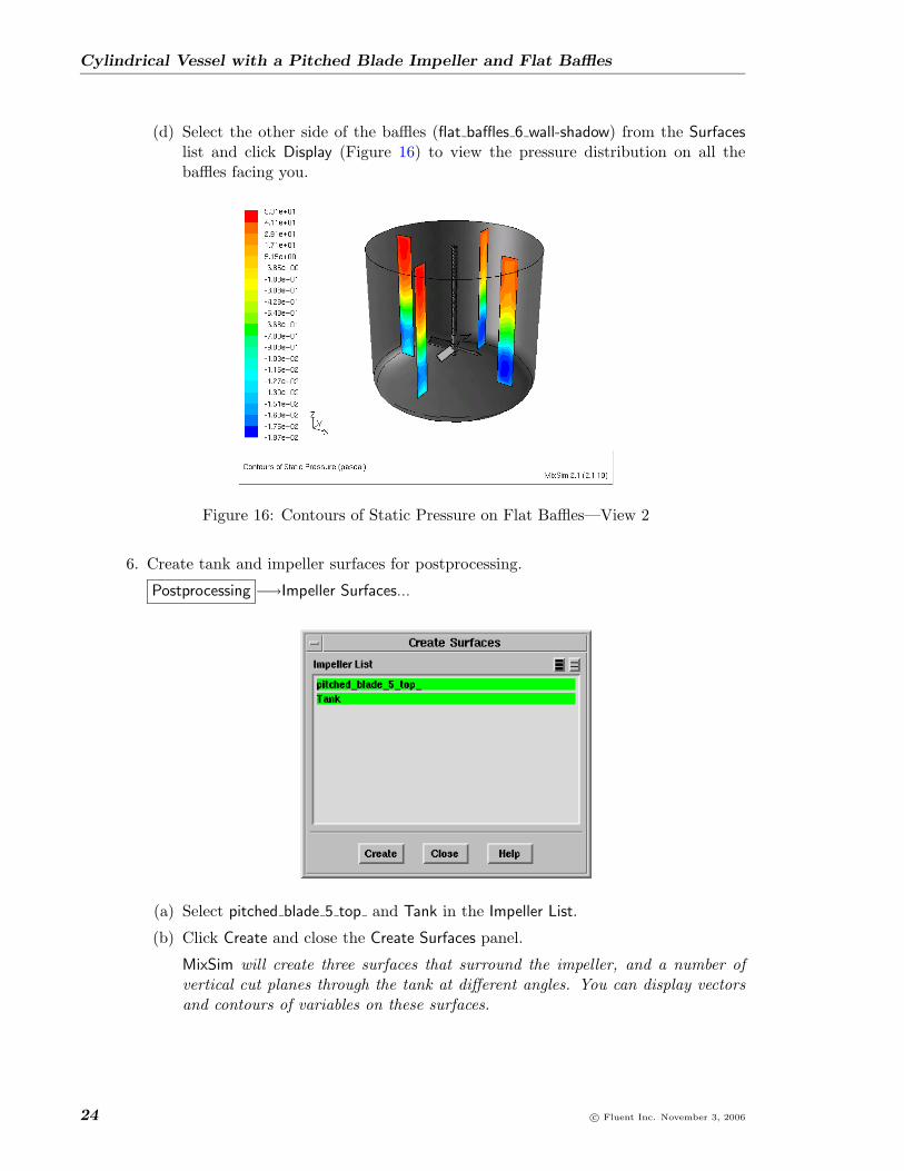
(d) Select the other side of the baffles (flat baffles 6 wall-shadow) from the Surfaceslist and click Display (Figure 16) to view the pressure distribution on all thebaffles facing you.

Figure 16: Contours of Static Pressure on Flat Baffles—View 2

6. Create tank and impeller surfaces for postprocessing.

Postprocessing −→Impeller Surfaces...

(a) Select pitched blade 5 top and Tank in the Impeller List.

(b) Click Create and close the Create Surfaces panel.

MixSim will create three surfaces that surround the impeller, and a number ofvertical cut planes through the tank at different angles. You can display vectorsand contours of variables on these surfaces.



7. Display contours of velocity in the fluid domain.

Display −→Contours...

(a) Select Velocity and Velocity Magnitude from the Contours of drop-down lists.

(b) Deselect the previously selected surfaces and select tank cut plane 60 degree fromthe Surfaces selection list.

(c) Disable the Lights On option and click Display to display the contours of velocityin the fluid domain (Figure 17).

Figure 17: Contours of Velocity in the Fluid Domain

8. Display velocity vectors on the vertical cut plane tank cut points 60 degree (Figure 18).

Velocity Vectors Colored By Velocity Magnitude (m/s)MixSim 2.1 (2.1.10)

1.23e+001.17e+001.11e+001.05e+009.90e-019.30e-018.70e-018.10e-017.50e-016.90e-016.31e-015.71e-015.11e-014.51e-013.91e-013.31e-012.71e-012.11e-011.51e-019.12e-023.13e-02

Z

YX

Figure 18: Velocity Vectors on the Cut Plane

You can try increasing the Scale setting in the MixSim Velocity Vectors panel.



9. Display the isosurface of velocity magnitude.

Postprocessing −→Iso Surface...

(a) Select Velocity and Velocity Magnitude from the Surface of Constant drop-downlists and click Compute.

The isovalues for Velocity Magnitude will be displayed in the Min and Max fields.

(b) Disable Faces in the Options group box in the MixSim Grid Display panel.

Display −→Grid...

(c) Move the Iso-Values slider from left to right to vary the isovalue from minimumto maximum (Figure 19).

Figure 19: Isosurface of Velocity Magnitude



As you move the slider, the graphics display is simultaneously updated. Thiswill help you in judging which part of the tank is poorly agitated. View thegraphic display simultaneously to see the isosurface for the corresponding isovalue(Figure 19).

10. Create a horizontal cut plane surface that is located exactly in the impeller plane.

You need to switch to the FLUENT user interface.

File −→Control Panel...

(a) Select Fluent from the Switch GUI menubar list.

(b) Close the Application Control Panel.

You will now have access to the FLUENT menu bar and all the commands inFLUENT.

(c) Open the Iso-Surface panel in FLUENT.

Surface −→Iso-Surface...

i. Select Grid... and Z-Coordinate from the Surface of Constant drop-down lists.



ii. Click Compute.

MixSim computes and displays the total range of z coordinate values.

iii. Enter 0.35 (the z coordinate of the horizontal impeller plane) for Iso-Values.

iv. Enter z=0.35 in the New Surface Name field.

v. Click Create and close the Iso-Surface panel.

(d) Switch back to the MixSim interface.

File −→Control Panel...

i. Select Mixsim from the Switch GUI menubar list.

ii. Close the Application Control Panel.

(e) Deselect the previously selected surfaces and select z=0.35 from the Surfaces listin the Contours panel.

(f) Enable Lights On, Show Tank, and Clear Colors in the Options group box.

(g) Click Display (Figure 20).

Figure 20: Contours of Velocity at the Impeller

11. Display a sweep surface.

Sweep surfaces allow you to dynamically create cut plane displays of contours or ve-locity vectors.

Display −→Sweep Surface...

(a) Select Contours in the Display Type list.

The Contours panel will open. Click the Properties... button if the panel does notopen automatically.



i. Select Pressure... and Static Pressure from the Contours of drop-down lists.

ii. Select the surfaces on which you want to see a contour plot together withthe sweep surface, e.g. the baffles.

iii. Click Compute.

MixSim will determine the minimum and maximum values for the chosenquantity that appear at any location of the selected surfaces. If you havenot selected any surface, the global maximum and minimum values will beidentified. If you want to specify the range of the color scale, disable AutoRange and enter appropriate values manually.

iv. Click OK to close the Contours panel.

(b) Move the horizontal slider located at the bottom of the Sweep Surface panel toview the surface sweeping throughout the tank domain (see Figures 21, 22, and23).

(c) Enter 1 for the Final Value in the Animation group box.

(d) Click the Animate button to animate the sweep surface.

You will see the contour plot displayed at 10 successive planes.

Notes:

• Moving the slider automatically updates the graphics display.

• All settings made in the MixSim Grid Display, Contours, or Vectors panels affectthe graphics display.

• The Contours and Vectors panels can be accessed through the Properties buttonin the Sweep Surface panel.

• To change the sweep direction, after entering vector component values in the X,Y, and Z fields, press <Enter> on your keyboard while the cursor is placed inany of the X, Y, or Z entry fields.



Figure 21: Contours of Pressure—Below the Impeller

Figure 22: Contours of Pressure—At the Impeller



Figure 23: Contours of Pressure—Above the Impeller

Step 10: Generating Reports

In addition to generating a correlations report, you can also create reports after the solutionis complete. These results are calculated from the numerical fluid flow (CFD) simulation(not from any correlations). Reports can be generated using the options in the Reportpull-down menu.

1. Report torque and power consumption values for the impeller.

Report −→Torque/Power



Select a Shaft and an Impeller to automatically update the displayed values. The Updatebutton allows you to force an update of the displayed values.

See Chapter 15: Examining the Solution for information on the other reports availablein MixSim.

2. Generate the HTML report for the MixSim model.

Report −→Generic Reports

(a) Select all the items in the Object List.

(b) Enter an appropriate file name in the File Name field.

You can use the Browse... button to select the location to save the file.

(c) Click Write.

(d) View the report in the browser.

The HTML report is shown in Figures 24—28. The report has been split across pagesfor better viewability. The report will appear as a continuous page in the browser.

Step 11: Exit

(a) Click Exit in the File menu to exit MixSim.

File −→Exit



Figure 24: HTML Report—Geometry and Model Objects List



Figure 25: HTML Report—Fluid Properties



Figure 26: HTML Report—Cylindrical Tank Parameters



Figure 27: HTML Report—Baffle and Shaft Parameters



Figure 28: HTML Report—Pitched Blade Parameters



Summary

By creating surfaces in the fluid domain, we can examine the flow field and can see highvelocities in the region around and below the impeller, with the velocity sharply decreasingin the radial direction. Very low velocities exist near the baffles and directly below theimpeller on the bottom of the vessel. These are the flow and velocity patterns expected ina mixing tank.

This tutorial has illustrated a typical problem-solving procedure using MixSim and has alsodemonstrated the how to analyze the model using postprocessing tools.


mixsim 2.1 tutorial -...

Documents