mixture of d-vine copulas for modeling dependence
TRANSCRIPT
Computational Statistics and Data Analysis 64 (2013) 1–19
Contents lists available at SciVerse ScienceDirect
Computational Statistics and Data Analysis
journal homepage: www.elsevier.com/locate/csda
Mixture of D-vine copulas for modeling dependenceDaeyoung Kim a, Jong-Min Kim b,∗, Shu-Min Liao c, Yoon-Sung Jung d
a Department of Mathematics and Statistics, University of Massachusetts, Amherst, MA 01003, USAb Statistic Discipline, Division of Science and Mathematics, University of Minnesota-Morris, Morris, MN 56267, USAc Department of Mathematics, Amherst College, Amherst, MA 01003, USAd Cooperative Agricultural Research Center, College of Agriculture and Human Sciences, Prairie View A&M University, Prairie View,TX 77446, USA
a r t i c l e i n f o
Article history:Received 24 June 2012Received in revised form 13 February 2013Accepted 14 February 2013Available online 5 March 2013
Keywords:DependenceMultivariate dataPair-copulaVines
a b s t r a c t
The identification of an appropriate multivariate copula for capturing the dependencestructure in multivariate data is not straightforward. The reason is because standardmultivariate copulas (such as the multivariate Gaussian, Student-t, and exchangeableArchimedean copulas) lack flexibility to model dependence and have other limitations,such as parameter restrictions. To overcome these problems, vine copulas have beendeveloped and applied to many applications. In order to reveal and fully understand thecomplex and hidden dependence patterns in multivariate data, amixture of D-vine copulasis proposed incorporating D-vine copulas into a finite mixture model. As a D-vine copulahas multiple parameters capturing the dependence through iterative construction of pair-copulas, the proposed model can facilitate a comprehensive study of complex and hiddendependence patterns in multivariate data. The proposed mixture of D-vine copulas isapplied to simulated and real data to illustrate its performance and benefits.
© 2013 Elsevier B.V. All rights reserved.
1. Introduction
Interest in copulas has been growing as statistical tools for understanding the dependence between several randomvariables, and copula-based modeling has been extensively applied to many areas including actuarial sciences (Carriére,2006), finance (Cherubini et al., 2004;McNeil et al., 2005), neuroscience (Onken et al., 2009), andweather research (Schölzeland Friederichs, 2008).
Copulas have several attractive properties. First, due to Sklar’s theorem (Sklar, 1959), copulas allowus tomodel separatelythe marginal distributions and the joint dependence structure. Second, they are invariant under increasing and continuoustransformations. Third, they do not require the marginals to be elliptically distributed, unlike correlation. Finally, copulascan be used to measure dependence in the tails of the joint distribution.
More importantly, the development of the vine copulas (Joe, 1996; Bedford and Cooke, 2001, 2002; Kurowicka and Cooke,2006; Aas et al., 2009) has been accelerating the use of the copula-basedmodeling to depict the dependence formultivariatedata. Vine copulas are a graphicalmodel designed to overcome the limitations of existing standardmultivariate copulas suchas the multivariate Gaussian, Student-t, and exchangeable Archimedean copulas. It is hierarchical in nature in the sensethat it can express a multivariate copula by using a cascade of bivariate copulas, the so-called pair-copulas. There are twopopular classes of vine copulas that have been widely used by many researchers: the canonical (C-) vine copulas and theD-vine copulas (Kurowicka and Cooke, 2004).
Recently there has been research that combine copulas with a finite mixture model in various areas of application to notonly fully understand the different dependence patterns between observed random variables, but also add more flexibility
∗ Corresponding author. Tel.: +1 320 589 6341; fax: +1 320 589 6371.E-mail addresses: [email protected], [email protected] (J.-M. Kim).
0167-9473/$ – see front matter© 2013 Elsevier B.V. All rights reserved.http://dx.doi.org/10.1016/j.csda.2013.02.018
2 D. Kim et al. / Computational Statistics and Data Analysis 64 (2013) 1–19
in terms of statistical modeling. By a finite mixture model, we mean a probabilistic model represented as a weighted sumof a few parametric densities. It is well known that the finite mixture model is very useful for uncovering hidden structuresin the data (Lindsay, 1995; McLachlan and Peel, 2000). For instance, Vrac et al. (2005) developed a mixture model of Frankcopulas to partition a global field of atmospheric profiles of temperature and humidity to characterize air masses whiletaking into account dependences between and among temperature and moisture through Frank copula functions. Cuvelierand Noirhomme-Fraiture (2005) proposed a mixture model of Clayton copulas for clustering in data mining, and showedthe Clayton copula based-mixture model provided equivalent or better results in terms of clustering compared to a mixtureof Normal copulas. Hu (2006) employed a mixture of three copulas, Gaussian, Gumbel and Gumbel-Survival, to modeldependence of monthly returns between a pair of stock indexes and capture left and/or right tail dependence.
Although useful, the aforementioned approaches to model heterogeneous dependence structures are unfortunatelylimited to bivariate data, and thus it is difficult to apply them to multivariate data with diverse dependence structures.As will be shown in Section 4.2, the four-dimensional precipitation data measured from four municipalities (Vestby, Ski,Hurdal and Nannestad) in Akershus County of Norway has two different dependence structures: one describing the overallpattern of precipitation in the Akershus Countywhile the other delineating dependence pattern of precipitation governed byeach location of the four municipalities. Note that none of the existing methods are developed to reveal these two differenttypes of dependence simultaneously.
In this paper we propose a mixture of D-vine copulas which includes multiple parameters for examining the differentdependences inherent in multivariate data and can be extended to a multivariate copula function. As one of the mostcommonly used vine copulas, a D-vine copula utilizes d(d − 1)/2 bivariate copula densities to express a d-dimensionalmultivariate density. By incorporating D-vine copulas into a finite mixture model, one can not only generate dependencestructures that may not belong to existing copula families, but also conduct a comprehensive study of complex and hiddendependence patterns in multivariate data. Note that a finite mixture model can also be viewed as a semiparametriccompromise between a fully parametric model (which often forces too much structure onto the data) and a nonparametricmodel (which leads to model estimates highly dependent on observed data). The reader will find from Section 4.2 thatthe proposed mixture of D-vine copulas successfully captures the diverse dependence structures hidden in multivariateprecipitation data mentioned above.
This article is organized as follows: Section 2 briefly reviews the D-vine copula and its full inference. Section 3 proposes afinite mixture model of D-vine copulas, describes the model estimation using the EM algorithm (Dempster et al., 1977), anddiscusses the model selection process. Section 4 shows the performance of the proposed mixture model of D-vine copulasin simulated data and real data. A brief discussion is then followed in Section 5.
2. D-vine copula
This section reviews the pair-copula decomposition of a multivariate distribution, the D-vine copula and its inferencepresented in Aas et al. (2009) and Aas and Berg (2009).
2.1. The pair-copula construction
Let X = (X1, . . . , Xd)′ be a d-dimensional random vector with the joint distribution function F = F(x1, . . . , xd) with
marginals F1 = F1(x1), . . . , Fd = Fd(xd). A copula is a function that allows us to represent the joint distribution in termsof its marginals and their dependence structure. Sklar’s theorem (Sklar, 1959) states that the copula associated with F is ad-dimensional distribution function C: [0, 1]d → [0, 1] that satisfies
F (x1, . . . , xd) = C (F1 (x1) , . . . , Fd (xd) ; β) , (1)
where β is the parameter vector measuring dependence between the marginals. For notational convenience, we will oftensuppress the parameter vector β.
For an absolutely continuous F with strictly increasing, continuous marginal densities F1, . . . , Fd, the joint densityfunction f is obtained from Eq. (1):
f (x1, . . . , xd) = c1···d (F1 (x1) , . . . , Fd (xd)) ·
dk=1
fk (xk) , (2)
where c1···d(·) is some uniquely identified d-variate copula density.Under suitable regularity conditions, one can represent a d-dimensional multivariate density in Eq. (2) as a product of
pair-copulas in an iterative manner, using the general form of a conditional marginal density in Eq. (3) (Aas et al., 2009):
f (xk|v) = cxk , vj|v−jFxk|v−j
, Fvj|v−j
· fxk|v−j
, (3)
where v = x−k is the (d − 1)-dimensional vector excluding xk, vj is any one component arbitrarily chosen from v, and v−jis the vector v excluding vj.
In the bivariate case (d = 2), the unconditional bivariate density and conditional density are
f (x1, x2) = c12 (F1 (x1) , F2 (x2)) f1 (x1) f2 (x2) , f (x1 | x2) = c12 (F1 (x1) , F2 (x2)) f1 (x1) ,
D. Kim et al. / Computational Statistics and Data Analysis 64 (2013) 1–19 3
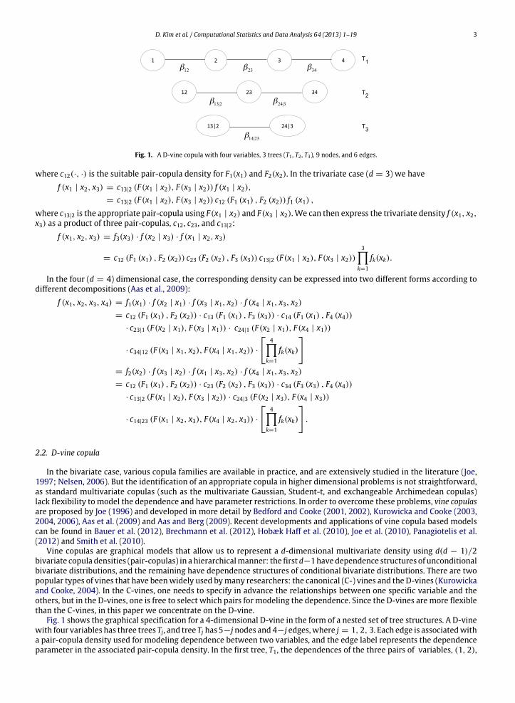
Fig. 1. A D-vine copula with four variables, 3 trees (T1 , T2 , T3), 9 nodes, and 6 edges.
where c12(·, ·) is the suitable pair-copula density for F1(x1) and F2(x2). In the trivariate case (d = 3) we havef (x1 | x2, x3) = c13|2 (F(x1 | x2), F(x3 | x2)) f (x1 | x2),
= c13|2 (F(x1 | x2), F(x3 | x2)) c12 (F1 (x1) , F2 (x2)) f1 (x1) ,
where c13|2 is the appropriate pair-copula using F(x1 | x2) and F(x3 | x2). We can then express the trivariate density f (x1, x2,x3) as a product of three pair-copulas, c12, c23, and c13|2:
f (x1, x2, x3) = f3(x3) · f (x2 | x3) · f (x1 | x2, x3)
= c12 (F1 (x1) , F2 (x2)) c23 (F2 (x2) , F3 (x3)) c13|2 (F(x1 | x2), F(x3 | x2))3
k=1
fk(xk).
In the four (d = 4) dimensional case, the corresponding density can be expressed into two different forms according todifferent decompositions (Aas et al., 2009):
f (x1, x2, x3, x4) = f1(x1) · f (x2 | x1) · f (x3 | x1, x2) · f (x4 | x1, x3, x2)= c12 (F1 (x1) , F2 (x2)) · c13 (F1 (x1) , F3 (x3)) · c14 (F1 (x1) , F4 (x4))
· c23|1 (F(x2 | x1), F(x3 | x1)) · c24|1 (F(x2 | x1), F(x4 | x1))
· c34|12 (F(x3 | x1, x2), F(x4 | x1, x2)) ·
4
k=1
fk(xk)
= f2(x2) · f (x3 | x2) · f (x1 | x3, x2) · f (x4 | x1, x3, x2)= c12 (F1 (x1) , F2 (x2)) · c23 (F2 (x2) , F3 (x3)) · c34 (F3 (x3) , F4 (x4))
· c13|2 (F(x1 | x2), F(x3 | x2)) · c24|3 (F(x2 | x3), F(x4 | x3))
· c14|23 (F(x1 | x2, x3), F(x4 | x2, x3)) ·
4
k=1
fk(xk)
.
2.2. D-vine copula
In the bivariate case, various copula families are available in practice, and are extensively studied in the literature (Joe,1997; Nelsen, 2006). But the identification of an appropriate copula in higher dimensional problems is not straightforward,as standard multivariate copulas (such as the multivariate Gaussian, Student-t, and exchangeable Archimedean copulas)lack flexibility to model the dependence and have parameter restrictions. In order to overcome these problems, vine copulasare proposed by Joe (1996) and developed in more detail by Bedford and Cooke (2001, 2002), Kurowicka and Cooke (2003,2004, 2006), Aas et al. (2009) and Aas and Berg (2009). Recent developments and applications of vine copula based modelscan be found in Bauer et al. (2012), Brechmann et al. (2012), Hobæk Haff et al. (2010), Joe et al. (2010), Panagiotelis et al.(2012) and Smith et al. (2010).
Vine copulas are graphical models that allow us to represent a d-dimensional multivariate density using d(d − 1)/2bivariate copula densities (pair-copulas) in a hierarchicalmanner: the first d−1havedependence structures of unconditionalbivariate distributions, and the remaining have dependence structures of conditional bivariate distributions. There are twopopular types of vines that have beenwidely used bymany researchers: the canonical (C-) vines and the D-vines (Kurowickaand Cooke, 2004). In the C-vines, one needs to specify in advance the relationships between one specific variable and theothers, but in the D-vines, one is free to select which pairs for modeling the dependence. Since the D-vines are more flexiblethan the C-vines, in this paper we concentrate on the D-vine.
Fig. 1 shows the graphical specification for a 4-dimensional D-vine in the form of a nested set of tree structures. A D-vinewith four variables has three trees Tj, and tree Tj has 5−jnodes and 4−j edges,where j = 1, 2, 3. Each edge is associatedwitha pair-copula density used for modeling dependence between two variables, and the edge label represents the dependenceparameter in the associated pair-copula density. In the first tree, T1, the dependences of the three pairs of variables, (1, 2),
4 D. Kim et al. / Computational Statistics and Data Analysis 64 (2013) 1–19
(2, 3), (3, 4), are modeled using three pair-copulas, c12(·; β12), c23(·; β23), and c34(·; β34). In the second tree, T2, two condi-tional dependences are modeled: (i) between the first and third variable given the second variable, the pair (1, 3 | 2), usingassociated pair-copula density c13|2(·; β13|2), and (ii) between the second and fourth variable given the third variable, the pair(2, 4 | 3), using associated pair-copula density c24|3(·; β24|3). Note that pairwise dependences of the two variables xa and xbwhere a, b = 1, . . . , d aremodeled in subsequent trees conditioned on those variables between the variables xa and xb in T1.
The d-dimensional D-vine density, given by Bedford and Cooke (2001), is
f (x; φ) =
dk=1
fk (xk)
×
d−1i=1
d−ij=1
cj,j+i|(j+1):(j+i−1)Fxj | xj+1, . . . , xj+i−1
, Fxj+i | xj+1, . . . , xj+i−1
; βj,j+i|(j+1):(j+i−1)
, (4)
where fk (xk) are themarginal densities, cj,j+i|(j+1):(j+i−1) are the bivariate copula densitieswith parameter(s)βj,j+i|(j+1):(j+i−1),and φ is the set of all parameters in the D-vine density.
In the four-dimensional case (d = 4), Eq. (4) then becomes
f (x1, x2, x3, x4; φ) = c12 (F(x1), F(x2); β12) · c23 (F(x2), F(x3); β23) · c34 (F(x3), F(x4); β34)
· c13|2F (x1 | x2) , F (x3 | x2) ; β13|2
· c24|3
F (x2 | x3) , F (x4 | x3) ; β24|3
· c14|23
F (x1 | x2, x3) , F (x4 | x2, x3) ; β14|23
·
4k=1
fk(xk),
where φ = (β12, β23, β34, β13|2, β24|3, β14|23).
2.3. Full inference for a D-vine copula
This section introduces the inference procedures of parameters in the D-vine density of Eq. (4). Assume that N observedsamples, say xk = (xk,1, . . . , xk,N), where k = 1, . . . , d, are available. Assume further that each random variable Xk is as-sumed to be uniform in [0,1] (so that fk(xk) = 1), which uses the normalized ranks of the original data for the parameterestimation. This is not a restrictive assumption because it is common that the distributions of the marginals are not knownin practice, and the normalized ranks of the data, which are only approximately uniform and independent, keep the largestamount of information about the joint dependence between the variables (Oakes, 1982).
Since statistical inference for a D-vine copula is based on the normalized ranks of the data, the method of maximumpseudo-likelihood for parameter estimation (Oakes, 1994; Genest et al., 1995; Shih and Louis, 1995; Kim et al., 2007) isadopted to maximize the log-pseudo likelihood for the D-vine density over the parameters:
ℓ(φ) =
d−1i=1
d−ij=1
Nn=1
log cj,j+i|(j+1):(j+i−1)
×Fxj,n | xj+1,n, . . . , xj+i−1,n
, Fxj+i,n | xj+1,n, . . . , xj+i−1,n
; βj,j+i|(j+1):(j+i−1)
, (5)
where φ is the set of all parameters in the D-vine density.In the case of a four-dimensional variables (d = 4), Eq. (5) becomes
ℓ(φ) =
Nn=1
log c12
x1,n, x2,n; β12
+ log c23
x2,n, x3,n; β23
+ log c34
x3,n, x4,n; β34
+ log c13|2
Fx1,n | x2,n
, Fx3,n | x2,n
; β13|2
+ log c24|3
Fx2,n | x3,n
, Fx4,n | x3,n
; β24|3
+ log c14|23
Fx1,n | x2,n, x3,n
, Fx4,n | x2,n, x3,n
; β14|23
,
where φ = (β12, β23, β34, β13|2, β24|3, β14|23).Full inference of a D-vine copula in Eq. (4) consists of three steps (Aas et al., 2009):
[Step 1] Choose which variables to include at the first tree T1 of a D-vine copula and decide the order of the variables using(tail) dependences (i.e., join the variables that have the strongest (tail) dependence).
[Step 2] Specify the parametric shape of each pair-copula in an assumed D-vine.[Step 3] Estimate all parameters of an assumed D-vine by numerically maximizing the log-pseudo likelihood in Eq. (5).
In [Step 1], one can find themost appropriate ordering of the variables by comparing Kendall’s tau values for all bivariatepairs (Aas et al., 2009; Aas and Berg, 2009). If there is information available on pair copula types for all pairs of a D-vinedensity, one can also choose the ordering of the variables by first fitting a specified bivariate copula to each pair, estimatingdependence parameters, and then comparing them (Aas et al., 2009).
D. Kim et al. / Computational Statistics and Data Analysis 64 (2013) 1–19 5
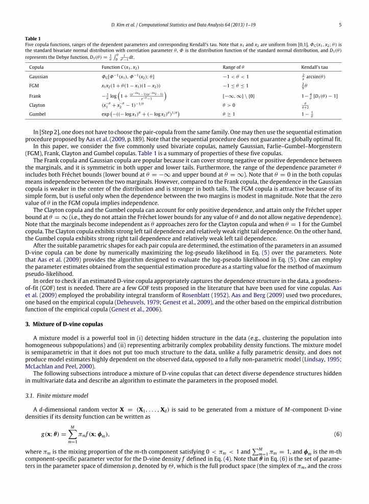
Table 1Five copula functions, ranges of the dependent parameters and corresponding Kendall’s tau. Note that x1 and x2 are uniform from [0,1], ΦG(x1, x2; θ) isthe standard bivariate normal distribution with correlation parameter θ , Φ is the distribution function of the standard normal distribution, and D1(θ)
represents the Debye function, D1(θ) =1θ
θ
0t
et−1 dt .
Copula Function C(x1, x2) Range of θ Kendall’s tau
Gaussian ΦG[Φ−1(x1), Φ−1(x2); θ ] −1 < θ < 1 2
πarcsin(θ)
FGM x1x2(1 + θ(1 − x1)(1 − x2)) −1 ≤ θ ≤ 1 29 θ
Frank −1θlog
1 +
(e−θx1 −1)(e−θx2 −1)e−θ −1
[−∞, ∞] \ 0 1−
4θ[D1(θ) − 1]
Clayton (x−θ1 + x−θ
2 − 1)−1/θ θ > 0 θθ+2
Gumbel exp−((− log x1)θ + (− log x2)θ )1/θ
θ ≥ 1 1 −
1θ
In [Step 2], one does not have to choose the pair-copula from the same family. Onemay then use the sequential estimationprocedure proposed by Aas et al. (2009, p.189). Note that the sequential procedure does not guarantee a globally optimal fit.
In this paper, we consider the five commonly used bivariate copulas, namely Gaussian, Farlie–Gumbel–Morgenstern(FGM), Frank, Clayton and Gumbel copulas. Table 1 is a summary of properties of these five copulas.
The Frank copula and Gaussian copula are popular because it can cover strong negative or positive dependence betweenthe marginals, and it is symmetric in both upper and lower tails. Furthermore, the range of the dependence parameter θincludes both Fréchet bounds (lower bound at θ = −∞ and upper bound at θ = ∞). Note that θ = 0 in the both copulasmeans independence between the twomarginals. However, compared to the Frank copula, the dependence in the Gaussiancopula is weaker in the center of the distribution and is stronger in both tails. The FGM copula is attractive because of itssimple form, but is useful only when the dependence between the two margins is modest in magnitude. Note that the zerovalue of θ in the FGM copula implies independence.
The Clayton copula and the Gumbel copula can account for only positive dependence, and attain only the Fréchet upperbound at θ = ∞ (i.e., they do not attain the Fréchet lower bounds for any value of θ and do not allow negative dependence).Note that the marginals become independent as θ approaches zero for the Clayton copula and when θ = 1 for the Gumbelcopula. The Clayton copula exhibits strong left tail dependence and relativelyweak right tail dependence. On the other hand,the Gumbel copula exhibits strong right tail dependence and relatively weak left tail dependence.
After the suitable parametric shapes for each pair copula are determined, the estimation of the parameters in an assumedD-vine copula can be done by numerically maximizing the log-pseudo likelihood in Eq. (5) over the parameters. Notethat Aas et al. (2009) provides the algorithm designed to evaluate the log-pseudo likelihood in Eq. (5). One can employthe parameter estimates obtained from the sequential estimation procedure as a starting value for themethod of maximumpseudo-likelihood.
In order to check if an estimated D-vine copula appropriately captures the dependence structure in the data, a goodness-of-fit (GOF) test is needed. There are a few GOF tests proposed in the literature that have been used for vine copulas. Aaset al. (2009) employed the probability integral transform of Rosenblatt (1952). Aas and Berg (2009) used two procedures,one based on the empirical copula (Deheuvels, 1979; Genest et al., 2009), and the other based on the empirical distributionfunction of the empirical copula (Genest et al., 2006).
3. Mixture of D-vine copulas
A mixture model is a powerful tool in (i) detecting hidden structure in the data (e.g., clustering the population intohomogeneous subpopulations) and (ii) representing arbitrarily complex probability density functions. The mixture modelis semiparametric in that it does not put too much structure to the data, unlike a fully parametric density, and does notproduce model estimates highly dependent on the observed data, opposed to a fully non-parametric model (Lindsay, 1995;McLachlan and Peel, 2000).
The following subsections introduce a mixture of D-vine copulas that can detect diverse dependence structures hiddenin multivariate data and describe an algorithm to estimate the parameters in the proposed model.
3.1. Finite mixture model
A d-dimensional random vector X = (X1, . . . ,Xd) is said to be generated from a mixture of M-component D-vinedensities if its density function can be written as
g(x; θ) =
Mm=1
πmf (x; φm), (6)
where πm is the mixing proportion of the m-th component satisfying 0 < πm < 1 andM
m=1 πm = 1, and φm is the m-thcomponent-specific parameter vector for the D-vine density f defined in Eq. (4). Note that θ in Eq. (6) is the set of parame-ters in the parameter space of dimension p, denoted by Θ , which is the full product space (the simplex of πm, and the cross
6 D. Kim et al. / Computational Statistics and Data Analysis 64 (2013) 1–19
product space of φm):
θ =
π1
φ1
, · · · ,
πm
φm
, · · · ,
πM
φM
, (7)
with each column corresponding to the parameters of each component. Here p is the total number of free parameters to beestimated, which is equal to (M − 1) +
Mm=1 dim(φm) where dim(a) denotes the dimension of a vector a.
Note that different column permutations of θ in Eq. (7) will give the same density g(x; θ) in Eq. (6), which is calledlabel-switching in mixture models. Therefore, we say that a mixture of M-component D-vine densities in Eq. (6) isidentifiable up to a column permutation of θ. See Lindsay (1995) and McLachlan and Peel (2000) for more details.
For the estimation of Eq. (6), both the number of components M and the parameters θ need to be estimated, which willbe addressed in the following two sections.
3.2. EM algorithm
In this section we describe the EM algorithm (Dempster et al., 1977) to obtain the estimates for the parameters θ in amixture of M-component D-vine densities, given the data set and the number of components M . The determination of Mwill be discussed later in Section 3.3.
Assume thatN observations, say xk = (xk,1, . . . , xk,N)where k = 1, . . . , d, drawn randomly from aM-component D-vinedensities in Eq. (6), are available. Then the log-likelihood of θ, ℓ(θ), is
ℓ(θ) = log
N
n=1
g(xn; θ)
= log
N
n=1
Mm=1
πmf (xn; φm)
. (8)
Let us denote latent variables zn = (zn1, . . . , znm, . . . , znM), where znm = 1 if xn comes from the m-th component andznm = 0 otherwise. Assume that zn is independent and identically distributed from a multinomial distribution, that is,zn ∼ Mult(M, π = (π1, . . . , πM)). The complete-data log likelihood for the complete data yn = (xn, zn), ℓc(θ), is given by
ℓc(θ) = logN
n=1
Mm=1
πmf (xn; φm)
znm=
Nn=1
Mm=1
znm logπm +
Nn=1
Mm=1
znm log f (xn; φm). (9)
The EM algorithm for estimating θ in a mixture of M-component D-vine densities is described as follows: Start with someinitial guess for the parameters, θ(0), and then repeat the E-step and M-step to compute successive estimates, θ(s) fors = 1, 2, . . . .[E-step] Computes the conditional expectation of the complete-data log likelihood, ℓc(θ) in Eq. (9), given the observed data
and current parameter estimates for θ. This is equivalent to the calculation of the posterior probability that xnbelongs to them-th component, given the current values of the parameters:
z(s)nm = E(znm | x, θ(s)) = P(znm = 1 | x, θ(s)) =
π(s)m f (xn; φ(s)
m )
Mℓ=1
π(s)ℓ f (xn; φ
(s)ℓ )
. (10)
[M-step]Compute the parameter estimates for each component independently, (π (s+1)1 , . . . , π
(s+1)m , . . . , π
(s+1)M ) and (φ
(s+1)1 ,
. . . , φ(s+1)m , . . . ,φ
(s+1)M ), by maximizing the expected complete-data log likelihood from the E-step. Here we can
obtain a closed-form solution for π(s+1)m : π
(s+1)m =
Nn=1 z(s)nmN . Then the estimation of φ(s+1)
m in the m-th componentD-vine density is equivalent to obtaining the parameter estimates weighted by z(s)
nm for the parameters in a D-vinedensity of Eq. (4). The optim function in the R software (R Development Core Team, 2012) is used to numericallymaximize the second term in Eq. (9) with respect to φm.
A nice property of the EM algorithm is that the log likelihood, ℓ(θ) in Eq. (8), is not decreased during the iteration:ℓ(θ(s+1)) ≥ ℓ(θ(s)). Thus, the E-step andM-step are iterateduntil ℓ(θ(s+1))−ℓ(θ(s)) is smaller than apredetermined tolerance,say 0.000001. For a detailed treatment of the convergence properties of EM algorithm, please see Dempster et al. (1977)and Wu (1983).
It is well known that the likelihood function for a finite mixture model has multiple local maximizers. Thus, we run theEM algorithm from multiple starting values for θ randomly selected from the range of the parameter space and choose alocal maximizer with the highest log likelihood among the found multiple local maximizers.
3.3. Model selection
Section 3.2 described how to estimate the parameters θ in Eq. (6). For full inference for a mixture model of D-vinedensities, however, (a) the determination of the number of componentsM and (b) the selection of pair-copula types in eachD-vine density are required. To these ends, we employ three widely used model selection criteria: Akaike’s information
D. Kim et al. / Computational Statistics and Data Analysis 64 (2013) 1–19 7
criterion (AIC) of Akaike (1973), the Bayesian information criterion (BIC) of Schwarz (1978), and the consistent AIC (CAIC)of Bozdogan (1987),
AIC = −2 log L(θ) + 2p,
BIC = −2 log L(θ) + p log(n),
CAIC = −2 log L(θ) + p(log(n) + 1),
where θ is the estimate of a p-dimensional θ in Eq. (6). Each criteria described above has two terms; the first term formeasuring the goodness-of-fit, and the second term for penalizing model complexity.
In practice, the number of components M is often determined by the model selection techniques, as the simulations inthe literature have shown that they can not only provide empirical evidence supporting the mixture model when the dataare heterogeneous, but also that they can help us avoid using over-parameterized models (see McLachlan and Peel (2000)for detailed reviews of simulation results). Note that the AIC tends to select more components than necessary even whenN is very large and a mixture model is correctly specified (Bozdogan, 1987; Celeux and Soromenho, 1996). The numericalexamples shown in Section 4 will illustrate this potential issue of the AIC.
As to the specification of pair-copula types in each D-vine density of a mixture model, it is not straightforward to employthe sequential estimation procedure proposed by Aas et al. (2009, p.189) (such as constructing pairwise scatter plots ofvariables and/or applying a GOF test for each pair of variables). This is because, in the context of the mixture model, theheterogeneity in the dependence structure is unobserved, and thus there is no observable information available regardingthe contribution of individual data points to unobserved heterogeneous dependence structures in the data. Thus, in thispaper, we employ the five commonly used bivariate copulas described in Table 1 of Section 2.3 (Gaussian, Frank, Clayton,Gumbel and FGM) as candidates of copula types for all pairs in a mixture of D-vine copulas.
In the numerical examples of Section 4, we will consider several candidates of a mixture of D-vine densities (generatedfrom five copula functions for all pairs and several values for the number of components) for given data, and identify abest-fit model by means of the model selection procedures described above.
We close this section by summarizing a procedure for the full inference of a mixture of D-vine copulas in Eq. (6):
[Step 1] Obtain the normalized ranks of the d-dimensional observed data.[Step 2] Decide the ordering of the variables at the first level (tree 1) of each D-vine density in a mixture of D-vine densities
by following a strategy proposed by Aas and Berg (2009): compute Kendall’s tau values for all bivariate pairs, andthe variables at tree 1 are ordered according to the (d − 1) largest Kendall’s tau values.
[Step 3] Consider various candidates of copulas for all pairs in an assumed model.[Step 4] Given a copula function chosen from the candidates of copula functions, fit a mixture of M-component D-vine
densities, withM ranging from 1 toM⋆ to the normalized data. Note that whenM = 1, a mixture ofM-componentD-vine densities is equivalent to the D-vine copulamodelwithout usingmixtures. If the number of copula functionsconsidered for the pair-copula is S, the number of mixture models fitted is S × M⋆. For the estimation of theparameters in each model, employ the EM algorithm described in Section 3.2.
[Step 5] Choose the best fitted model (the final pair-copula type for all pairs and the value of M) among the fitted modelsby finding the model with the smallest values of the model selection measures such as the AIC, BIC, and CAIC.
4. Numerical examples
In this section the performance of the proposed mixture of D-vine copulas is illustrated with numerous simulatedexamples and with a real data set studied in Aas and Berg (2009). The results of model estimation are presented in aform of the tree structure as shown in Fig. 1, with the dependence parameter in each pair-copula term at the edge andthe corresponding Kendall’s tau value in parenthesis.
4.1. Simulation studies
The results from the simulation examples are presented in three subsections. In the first subsection the focus is on thescenario where the data generating process (DGP) is a mixture of D-vine copulas in order to check whether the proposedmodel is able to capture different patterns of dependence structures hidden in themultivariate data. In the second and thirdsubsection, the focus is on the model misspecification scenario. The second subsection is concerned with the case wherethe DGP is a single-component multivariate D-vine copula which does not have any meaningful mixture of dependences,but a mixture of D-vine copulas is fitted to the data. This scenario will investigate the effect of the misspecificationon the number of components. The third subsection studies the performance of the proposed model when the DGP ismisspecified; more specifically, we study the case when the data are generated from amixture of multivariate skew normaldistributions (Azzalini and Capitanio, 1999), rather than a mixture of D-vine copulas.
For the data simulation, the CDVineSim function in the R package CDVine (Brechmann and Schepsmeier, 2011) is usedin the first two subsections and the rmsn function in the R package sn (Azzalini, 2011) is used in the third subsection.
8 D. Kim et al. / Computational Statistics and Data Analysis 64 (2013) 1–19
(a) Case 1.
(b) Case 2.
(c) Case 3.
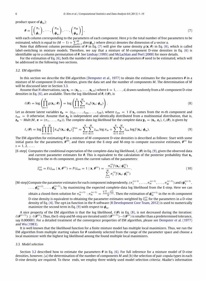
Fig. 2. Simulation models for three cases: (a) Case 1 — a mixture of Frank based D-vine copulas with two components, the first one with only negativedependence and the second one with only positive dependence, (b) Case 2 — a mixture of Clayton based D-vine copulas with two components, the firstone with weak positive dependence and the second one with strong positive dependence, and (c) Case 3 — a mixture of Frank based D-vine copulas withthree components, the first one with only negative dependence, the second one with only positive dependence and the third one with both positive andnegative dependences. Note that the values at each edge are the true value of the parameter (outside the parenthesis) and the corresponding Kendall tauvalue (inside the parenthesis).
4.1.1. Cases with a mixture of D-vine copulasWe here illustrate applications of a mixture of D-vine copulas to three sets of simulated data representing different
types of dependence structure. The first two sets of simulated data, denoted by Case 1 and Case 2, are the cases where theobservations are generated from a two-component (M = 2) mixture of three-dimensional (d = 3) D-vine densities withFrank and Clayton copulas for all pairs, respectively. The third set of simulated data, denoted by Case 3, is the case wherethere are three different dependence structures generated from a three-component (M = 3) mixture of three-dimensional(d = 3) D-vine densities with Frank copulas for all pairs.
Fig. 2 shows three simulation models (Case 1, Case 2, Case 3) in the form of tree structures. Fig. 2 (a) (Case 1) shows atwo-componentmixture of three dimensional Frank copula-based D-vine densities with equalmixing proportions (π1 = π2= 0.5), where the first component has only negative dependences and the second component has only positive depen-dences. Fig. 2 (b) (Case 2) is a mixture of Clayton-based D-vine densities with two components (π1 = π2 = 0.5), one withweak positive dependence and the other with strong positive dependence. Fig. 2 (c) (Case 3) represents a mixture of Frankcopula-based D-vine densities with three components (π1 = π2 = 0.3, π3 = 0.4), and has more challenging dependencestructures than those of Case 1. The third component of this last simulation model contains both positive and negativedependence.
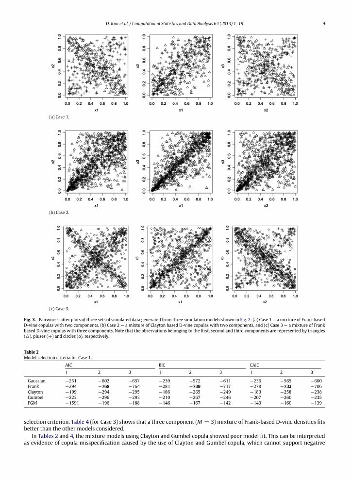
Fig. 3 gives pairwise scatter plots for three sets of data simulated from the three simulation models given in Fig. 2. Thenumber of observations (N) simulated from the threemixturemodels are 500 for Case 1, 1000 for Case 2 and 1000 for Case 3,respectively. Let Tmj be the j-th tree of the m-th component. The observations generated from the first component D-vinedensity (T11, T12) and the second component D-vine density (T21, T22) are represented by triangles () and pluses (+),respectively. The observations generated from the third component (T31, T32) in Case 3 are represented by circles (o).
In order to find a best fittedmodel to each data set, we consider the five copula functions (Gaussian, FGM, Frank, Clayton,and Gumbel) as candidates for all pair-copulas in a mixture of D-vine densities, with the number of components rangingfrom1 toM∗. For Case 1 and 2,we setM∗
= 3, and for Case 3, setM∗= 4. Thenwe compute themodel selection criteria (AIC,
BIC, CAIC) at each fittedmodel. Note that we employ amultiple starting value strategy in the EM algorithmwhen estimatingthe parameters in an assumed model.
Tables 2–4 provide the results for the model selection in the three sets of simulated data. Note that Boldface indicatesthe number of components and pair-copula type selected by each criterion. As shown in Table 2 (for Case 1) and Table 3(for Case 2), a two-component (M = 2) mixture of Frank (for Case 1) and Clayton (for Case 2) based D-vine densities isbetter fitted to simulated data than the other models we considered because it has the smallest values for each of the model
D. Kim et al. / Computational Statistics and Data Analysis 64 (2013) 1–19 9
(a) Case 1.
(b) Case 2.
(c) Case 3.
Fig. 3. Pairwise scatter plots of three sets of simulated data generated from three simulationmodels shown in Fig. 2: (a) Case 1 — amixture of Frank basedD-vine copulas with two components, (b) Case 2 — a mixture of Clayton based D-vine copulas with two components, and (c) Case 3 — a mixture of Frankbased D-vine copulas with three components. Note that the observations belonging to the first, second and third components are represented by triangles(), pluses (+) and circles (o), respectively.
Table 2Model selection criteria for Case 1.
AIC BIC CAIC1 2 3 1 2 3 1 2 3
Gaussian −251 −602 −657 −239 −572 −611 −236 −565 −600Frank −294 −768 −764 −281 −739 −717 −278 −732 −706Clayton −199 −294 −295 −186 −265 −249 −183 −258 −238Gumbel −223 −296 −293 −210 −267 −246 −207 −260 −235FGM −1591 −196 −188 −146 −167 −142 −143 −160 −139
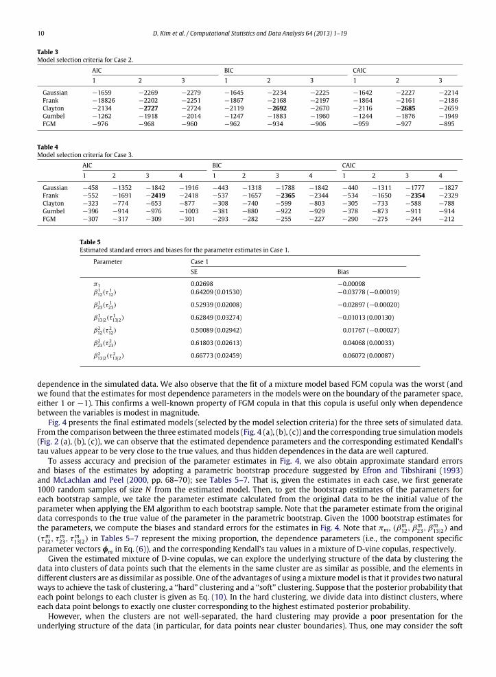
selection criterion. Table 4 (for Case 3) shows that a three component (M = 3) mixture of Frank-based D-vine densities fitsbetter than the other models considered.
In Tables 2 and 4, the mixture models using Clayton and Gumbel copula showed poor model fit. This can be interpretedas evidence of copula misspecification caused by the use of Clayton and Gumbel copula, which cannot support negative
10 D. Kim et al. / Computational Statistics and Data Analysis 64 (2013) 1–19
Table 3Model selection criteria for Case 2.
AIC BIC CAIC1 2 3 1 2 3 1 2 3
Gaussian −1659 −2269 −2279 −1645 −2234 −2225 −1642 −2227 −2214Frank −18826 −2202 −2251 −1867 −2168 −2197 −1864 −2161 −2186Clayton −2134 −2727 −2724 −2119 −2692 −2670 −2116 −2685 −2659Gumbel −1262 −1918 −2014 −1247 −1883 −1960 −1244 −1876 −1949FGM −976 −968 −960 −962 −934 −906 −959 −927 −895
Table 4Model selection criteria for Case 3.
AIC BIC CAIC1 2 3 4 1 2 3 4 1 2 3 4
Gaussian −458 −1352 −1842 −1916 −443 −1318 −1788 −1842 −440 −1311 −1777 −1827Frank −552 −1691 −2419 −2418 −537 −1657 −2365 −2344 −534 −1650 −2354 −2329Clayton −323 −774 −653 −877 −308 −740 −599 −803 −305 −733 −588 −788Gumbel −396 −914 −976 −1003 −381 −880 −922 −929 −378 −873 −911 −914FGM −307 −317 −309 −301 −293 −282 −255 −227 −290 −275 −244 −212
Table 5Estimated standard errors and biases for the parameter estimates in Case 1.
Parameter Case 1SE Bias
π1 0.02698 −0.00098β112(τ
112) 0.64209 (0.01530) −0.03778 (−0.00019)
β123(τ
123) 0.52939 (0.02008) −0.02897 (−0.00020)
β113|2(τ
113|2) 0.62849 (0.03274) −0.01013 (0.00130)
β212(τ
212) 0.50089 (0.02942) 0.01767 (−0.00027)
β223(τ
223) 0.61803 (0.02613) 0.04068 (0.00033)
β213|2(τ
213|2) 0.66773 (0.02459) 0.06072 (0.00087)
dependence in the simulated data. We also observe that the fit of a mixture model based FGM copula was the worst (andwe found that the estimates for most dependence parameters in the models were on the boundary of the parameter space,either 1 or −1). This confirms a well-known property of FGM copula in that this copula is useful only when dependencebetween the variables is modest in magnitude.
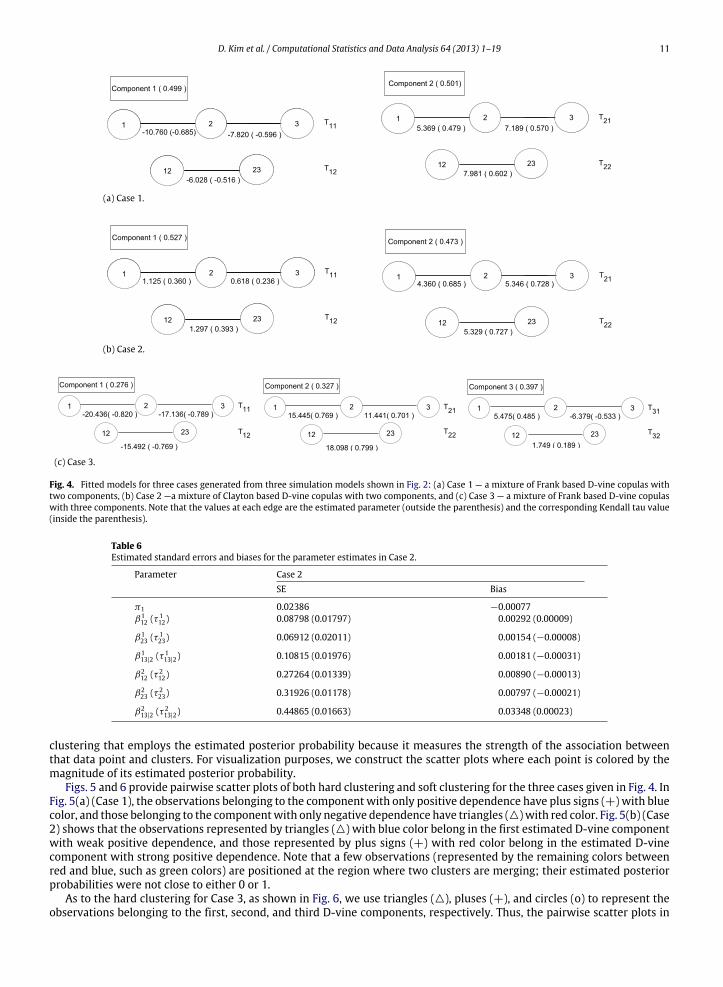
Fig. 4 presents the final estimated models (selected by the model selection criteria) for the three sets of simulated data.From the comparison between the three estimatedmodels (Fig. 4 (a), (b), (c)) and the corresponding true simulationmodels(Fig. 2 (a), (b), (c)), we can observe that the estimated dependence parameters and the corresponding estimated Kendall’stau values appear to be very close to the true values, and thus hidden dependences in the data are well captured.
To assess accuracy and precision of the parameter estimates in Fig. 4, we also obtain approximate standard errorsand biases of the estimates by adopting a parametric bootstrap procedure suggested by Efron and Tibshirani (1993)and McLachlan and Peel (2000, pp. 68–70); see Tables 5–7. That is, given the estimates in each case, we first generate1000 random samples of size N from the estimated model. Then, to get the bootstrap estimates of the parameters foreach bootstrap sample, we take the parameter estimate calculated from the original data to be the initial value of theparameter when applying the EM algorithm to each bootstrap sample. Note that the parameter estimate from the originaldata corresponds to the true value of the parameter in the parametric bootstrap. Given the 1000 bootstrap estimates forthe parameters, we compute the biases and standard errors for the estimates in Fig. 4. Note that πm, (βm
12, βm23, β
m13|2) and
(τm12, τ
m23, τ
m13|2) in Tables 5–7 represent the mixing proportion, the dependence parameters (i.e., the component specific
parameter vectors φm in Eq. (6)), and the corresponding Kendall’s tau values in a mixture of D-vine copulas, respectively.Given the estimated mixture of D-vine copulas, we can explore the underlying structure of the data by clustering the
data into clusters of data points such that the elements in the same cluster are as similar as possible, and the elements indifferent clusters are as dissimilar as possible. One of the advantages of using amixturemodel is that it provides two naturalways to achieve the task of clustering, a ‘‘hard’’ clustering and a ‘‘soft’’ clustering. Suppose that the posterior probability thateach point belongs to each cluster is given as Eq. (10). In the hard clustering, we divide data into distinct clusters, whereeach data point belongs to exactly one cluster corresponding to the highest estimated posterior probability.
However, when the clusters are not well-separated, the hard clustering may provide a poor presentation for theunderlying structure of the data (in particular, for data points near cluster boundaries). Thus, one may consider the soft
D. Kim et al. / Computational Statistics and Data Analysis 64 (2013) 1–19 11
(a) Case 1.
(b) Case 2.
(c) Case 3.
Fig. 4. Fitted models for three cases generated from three simulation models shown in Fig. 2: (a) Case 1 — a mixture of Frank based D-vine copulas withtwo components, (b) Case 2 —a mixture of Clayton based D-vine copulas with two components, and (c) Case 3 — a mixture of Frank based D-vine copulaswith three components. Note that the values at each edge are the estimated parameter (outside the parenthesis) and the corresponding Kendall tau value(inside the parenthesis).
Table 6Estimated standard errors and biases for the parameter estimates in Case 2.
Parameter Case 2SE Bias
π1 0.02386 −0.00077β112 (τ 1
12) 0.08798 (0.01797) 0.00292 (0.00009)
β123 (τ 1
23) 0.06912 (0.02011) 0.00154 (−0.00008)
β113|2 (τ 1
13|2) 0.10815 (0.01976) 0.00181 (−0.00031)
β212 (τ 2
12) 0.27264 (0.01339) 0.00890 (−0.00013)
β223 (τ 2
23) 0.31926 (0.01178) 0.00797 (−0.00021)
β213|2 (τ 2
13|2) 0.44865 (0.01663) 0.03348 (0.00023)
clustering that employs the estimated posterior probability because it measures the strength of the association betweenthat data point and clusters. For visualization purposes, we construct the scatter plots where each point is colored by themagnitude of its estimated posterior probability.
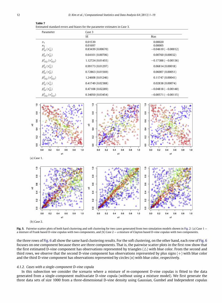
Figs. 5 and 6 provide pairwise scatter plots of both hard clustering and soft clustering for the three cases given in Fig. 4. InFig. 5(a) (Case 1), the observations belonging to the component with only positive dependence have plus signs (+) with bluecolor, and those belonging to the componentwith only negative dependence have triangles ()with red color. Fig. 5(b) (Case2) shows that the observations represented by triangles () with blue color belong in the first estimated D-vine componentwith weak positive dependence, and those represented by plus signs (+) with red color belong in the estimated D-vinecomponent with strong positive dependence. Note that a few observations (represented by the remaining colors betweenred and blue, such as green colors) are positioned at the region where two clusters are merging; their estimated posteriorprobabilities were not close to either 0 or 1.
As to the hard clustering for Case 3, as shown in Fig. 6, we use triangles (), pluses (+), and circles (o) to represent theobservations belonging to the first, second, and third D-vine components, respectively. Thus, the pairwise scatter plots in
12 D. Kim et al. / Computational Statistics and Data Analysis 64 (2013) 1–19
Table 7Estimated standard errors and biases for the parameter estimates in Case 3.
Parameter Case 3SE Bias
π1 0.01539 0.00020π2 0.01697 0.00005β112 (τ 1
12) 0.83439 (0.00670) −0.04610 (−0.00012)
β123 (τ 1
23) 0.64101 (0.00706) 0.00760 (0.00032)
β113|2 (τ 1
13|2) 1.12724 (0.01455) −0.17388 (−0.00136)
β212 (τ 2
12) 0.99173 (0.01297) 0.06814 (0.00018)
β223 (τ 2
23) 0.72863 (0.01569) 0.06007 (0.00051)
β213|2 (τ 2
13|2) 1.24608 (0.01246) 0.11747 (0.00041)
β312 (τ 3
12) 0.41749 (0.02388) 0.02838 (0.00074)
β323 (τ 3
23) 0.47108 (0.02289) −0.04818 (−0.00140)
β313|2 (τ 3
13|2) 0.34050 (0.03454) −0.00571 (−0.00115)
(a) Case 1.
(b) Case 2.
Fig. 5. Pairwise scatter plots of both hard clustering and soft clustering for two cases generated from two simulation models shown in Fig. 2: (a) Case 1 —a mixture of Frank based D-vine copulas with two components, and (b) Case 2 — a mixture of Clayton based D-vine copulas with two components.
the three rows of Fig. 6 all show the same hard clustering results. For the soft clustering, on the other hand, each row of Fig. 6focuses on one component because there are three components. That is, the pairwise scatter plots in the first row show thatthe first estimated D-vine component has observations represented by triangles () with blue color. From the second andthird rows, we observe that the second D-vine component has observations represented by plus signs (+) with blue colorand the third D-vine component has observations represented by circles (o) with blue color, respectively.
4.1.2. Cases with a single-component D-vine copulaIn this subsection we consider the scenario where a mixture of m-component D-vine copulas is fitted to the data
generated from a single-component multivariate D-vine copula (without using a mixture model). We first generate thethree data sets of size 1000 from a three-dimensional D-vine density using Gaussian, Gumbel and Independent copulas
D. Kim et al. / Computational Statistics and Data Analysis 64 (2013) 1–19 13
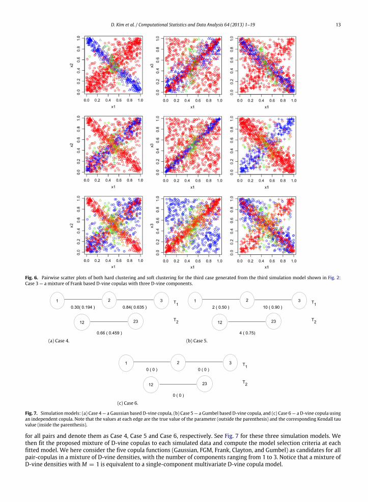
Fig. 6. Pairwise scatter plots of both hard clustering and soft clustering for the third case generated from the third simulation model shown in Fig. 2:Case 3 — a mixture of Frank based D-vine copulas with three D-vine components.
(a) Case 4. (b) Case 5.
(c) Case 6.
Fig. 7. Simulationmodels: (a) Case 4 — a Gaussian based D-vine copula, (b) Case 5 — a Gumbel based D-vine copula, and (c) Case 6 — a D-vine copula usingan independent copula. Note that the values at each edge are the true value of the parameter (outside the parenthesis) and the corresponding Kendall tauvalue (inside the parenthesis).
for all pairs and denote them as Case 4, Case 5 and Case 6, respectively. See Fig. 7 for these three simulation models. Wethen fit the proposed mixture of D-vine copulas to each simulated data and compute the model selection criteria at eachfitted model. We here consider the five copula functions (Gaussian, FGM, Frank, Clayton, and Gumbel) as candidates for allpair-copulas in a mixture of D-vine densities, with the number of components ranging from 1 to 3. Notice that a mixture ofD-vine densities withM = 1 is equivalent to a single-component multivariate D-vine copula model.
14 D. Kim et al. / Computational Statistics and Data Analysis 64 (2013) 1–19
Table 8Model selection criteria for Case 4.
AIC BIC CAIC1 2 3 1 2 3 1 2 3
Gaussian −2002 −1997 −1991 −1987 −1963 −1937 −1984 −1956 −1926Frank −1759 −1765 −1761 −1744 −1731 −1707 −1741 −1724 −1696Clayton −1456 −1530 −1542 −1441 −1495 −1488 −1438 −1488 −1477Gumbel −1753 −1770 −1765 −1738 −1736 −1711 −1735 −1729 −1700FGM −709 −701 −693 −694 −666 −639 −691 −659 −628
Table 9Model selection criteria for Case 5.
AIC BIC CAIC1 2 3 1 2 3 1 2 3
Gaussian −5823 −6083 −6120 −5809 −6049 −6066 −5806 −6042 −6055Frank −5511 −5669 −5692 −5496 −5634 −5638 −5493 −5627 −5627Clayton −3539 −4452 −4573 −3525 −4417 −4519 −3522 −4410 −4508Gumbel −6583 −6582 −6575 −6569 −6548 −6521 −6566 −6541 −6510FGM −1051 −1043 −1035 −1036 −1008 −981 −1033 −1001 −970
Table 10Model selection criteria for Case 6.
AIC BIC CAIC1 2 3 1 2 3 1 2 3
Gaussian 1.716 −0.58 −1.59 16.44 33.78 52.40 19.44 40.78 63.40Frank 2.15 0.74 −6.53 16.88 35.09 47.45 19.88 42.09 58.45Clayton 0.98 7.84 15.52 15.70 42.19 69.51 18.70 49.19 80.51Gumbel 2.60 6.09 13.48 17.33 40.45 67.47 20.33 47.45 78.47FGM 2.09 2.31 8.13 16.82 36.66 62.12 19.82 43.66 73.12
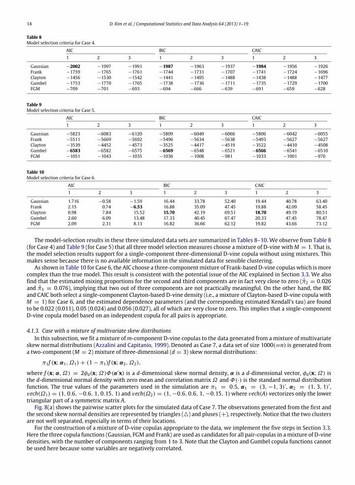
The model-selection results in these three simulated data sets are summarized in Tables 8–10. We observe from Table 8(for Case 4) and Table 9 (for Case 5) that all three model selection measures choose a mixture of D-vine withM = 1. That is,the model selection results support for a single-component three-dimensional D-vine copula without using mixtures. Thismakes sense because there is no available information in the simulated data for sensible clustering.
As shown in Table 10 for Case 6, the AIC choose a three-componentmixture of Frank-based D-vine copulas which is morecomplex than the true model. This result is consistent with the potential issue of the AIC explained in Section 3.3. We alsofind that the estimated mixing proportions for the second and third components are in fact very close to zero (π2 = 0.026and π3 = 0.076), implying that two out of three components are not practically meaningful. On the other hand, the BICand CAIC both select a single-component Clayton-based D-vine density (i.e., a mixture of Clayton-based D-vine copula withM = 1) for Case 6, and the estimated dependence parameters (and the corresponding estimated Kendall’s tau) are foundto be 0.022 (0.011), 0.05 (0.024) and 0.056 (0.027), all of which are very close to zero. This implies that a single-componentD-vine copula model based on an independent copula for all pairs is appropriate.
4.1.3. Case with a mixture of multivariate skew distributionsIn this subsection, we fit a mixture ofm-component D-vine copulas to the data generated from amixture of multivariate
skew normal distributions (Azzalini and Capitanio, 1999). Denoted as Case 7, a data set of size 1000(=n) is generated froma two-component (M = 2) mixture of three-dimensional (d = 3) skew normal distributions:
π1f (x; α1, Ω1) + (1 − π1)f (x; α2, Ω2),
where f (x; α, Ω) = 2φd(x; Ω)Φ(α′x) is a d-dimensional skew normal density, α is a d-dimensional vector, φd(x; Ω) isthe d-dimensional normal density with zero mean and correlation matrix Ω and Φ(·) is the standard normal distributionfunction. The true values of the parameters used in the simulation are π1 = 0.5, α1 = (3, −1, 3)′, α2 = (1, 3, 1)′,vech(Ω1) = (1, 0.6, −0.6, 1, 0.15, 1) and vech(Ω2) = (1, −0.6, 0.6, 1, −0.15, 1)where vech(A) vectorizes only the lowertriangular part of a symmetric matrix A.
Fig. 8(a) shows the pairwise scatter plots for the simulated data of Case 7. The observations generated from the first andthe second skew normal densities are represented by triangles () and pluses (+), respectively. Notice that the two clustersare not well separated, especially in terms of their locations.
For the construction of a mixture of D-vine copulas appropriate to the data, we implement the five steps in Section 3.3.Here the three copula functions (Gaussian, FGM and Frank) are used as candidates for all pair-copulas in a mixture of D-vinedensities, with the number of components ranging from 1 to 3. Note that the Clayton and Gumbel copula functions cannotbe used here because some variables are negatively correlated.
D. Kim et al. / Computational Statistics and Data Analysis 64 (2013) 1–19 15
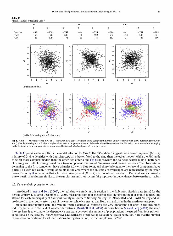
Table 11Model selection criteria for Case 7.
AIC BIC CAIC1 2 3 1 2 3 1 2 3
Gaussian −59 −758 −768 −44 −724 −714 −41 −717 −703Frank −50 −626 −636 −36 −592 −582 −33 −585 −571FGM −45 −179 −171 −30 −145 −117 −27 −138 −106
(a) Simulated data.
(b) Hard clustering and soft clustering.
Fig. 8. Case 7 — pairwise scatter plots of (a) simulated data generated from a two-component mixture of three-dimensional skew normal distributions,and (b) hard clustering and soft clustering based on a two-component mixture of Gaussian-based D-vine densities. Note that the observations belongingto the first and second components are represented by triangles () and pluses (+), respectively.
Table 11 provides the results for themodel selection for Case 7. The BIC and CAIC suggest that a two-component (M = 2)mixture of D-vine densities with Gaussian copulas is better fitted to the data than the other models, while the AIC tendsto select more complex models than the other two criteria did. Fig. 8 (b) provides the pairwise scatter plots of both hardclustering and soft clustering based on a two-component mixture of Gaussian-based D-vine densities. The observationsbelonging to the first component have triangles () with blue color, and those belonging to the second component havepluses (+) with red color. A group of points in the area where the clusters are overlapped are represented by the greencolors. From Fig. 8 we observe that a fitted two-component (M = 2) mixture of Gaussian-based D-vine densities providesthe two estimated clusters similar to the true clusters and thus successfully captures the dependences between the variables.
4.2. Data analysis: precipitation data
Introduced in Aas and Berg (2009), the real data we study in this section is the daily precipitation data (mm) for theperiod January 1, 1990 to December 31, 2006, measured from four meteorological stations in the four municipalities, onestation for each municipality of Akershus County in southern Norway: Vestby, Ski, Nannestad, and Hurdal. Vestby and Skiare located in the southwestern part of the county, while Nannestad and Hurdal are situated in the northwestern part.
Modeling precipitation data and valuing related derivative contracts are very important not only in the insuranceindustry, but also in the field of weather derivatives (Musshoff et al., 2006). As described in Aas and Berg (2009), the maininterest here is to estimate the dependence structure between the amount of precipitations measured from four stations,conditional on that it rains. Thus,we remove dayswith zero precipitation values for at least one station. Note that the numberof non-zero precipitation for all four stations during this period, i.e. the sample size, is 2065.
16 D. Kim et al. / Computational Statistics and Data Analysis 64 (2013) 1–19
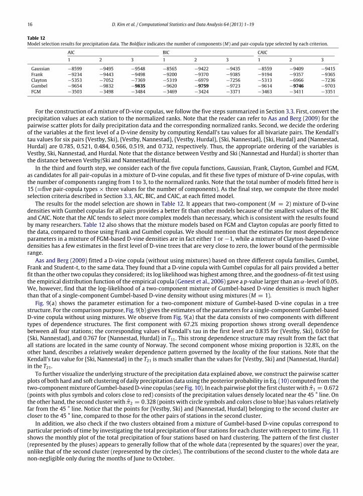
Table 12Model selection results for precipitation data. The Boldface indicates the number of components (M) and pair-copula type selected by each criterion.
AIC BIC CAIC1 2 3 1 2 3 1 2 3
Gaussian −8599 −9495 −9548 −8565 −9422 −9435 −8559 −9409 −9415Frank −9234 −9443 −9498 −9200 −9370 −9385 −9194 −9357 −9365Clayton −5353 −7052 −7369 −5319 −6979 −7256 −5313 −6966 −7236Gumbel −9654 −9832 −9835 −9620 −9759 −9723 −9614 −9746 −9703FGM −3503 −3498 −3484 −3469 −3424 −3371 −3463 −3411 −3351
For the construction of a mixture of D-vine copulas, we follow the five steps summarized in Section 3.3. First, convert theprecipitation values at each station to the normalized ranks. Note that the reader can refer to Aas and Berg (2009) for thepairwise scatter plots for daily precipitation data and the corresponding normalized ranks. Second, we decide the orderingof the variables at the first level of a D-vine density by computing Kendall’s tau values for all bivariate pairs. The Kendall’stau values for six pairs Vestby, Ski, Vestby, Nannestad, Vestby, Hurdal, Ski, Nannestad, Ski, Hurdal and Nannestad,Hurdal are 0.785, 0.521, 0.484, 0.566, 0.519, and 0.732, respectively. Thus, the appropriate ordering of the variables isVestby, Ski, Nannestad, and Hurdal. Note that the distance between Vestby and Ski (Nannestad and Hurdal) is shorter thanthe distance between Vestby/Ski and Nannestad/Hurdal.
In the third and fourth step, we consider each of the five copula functions, Gaussian, Frank, Clayton, Gumbel and FGM,as candidates for all pair-copulas in a mixture of D-vine copulas, and fit these five types of mixture of D-vine copulas, withthe number of components ranging from 1 to 3, to the normalized ranks. Note that the total number of models fitted here is15 (=five pair-copula types × three values for the number of components). As the final step, we compute the three modelselection criteria described in Section 3.3, AIC, BIC, and CAIC, at each fitted model.
The results for the model selection are shown in Table 12. It appears that two-component (M = 2) mixture of D-vinedensities with Gumbel copulas for all pairs provides a better fit than other models because of the smallest values of the BICand CAIC. Note that the AIC tends to select more complex models than necessary, which is consistent with the results foundby many researchers. Table 12 also shows that the mixture models based on FGM and Clayton copulas are poorly fitted tothe data, compared to those using Frank and Gumbel copulas. We should mention that the estimates for most dependenceparameters in a mixture of FGM-based D-vine densities are in fact either 1 or −1, while a mixture of Clayton-based D-vinedensities has a few estimates in the first level of D-vine trees that are very close to zero, the lower bound of the permissiblerange.
Aas and Berg (2009) fitted a D-vine copula (without using mixtures) based on three different copula families, Gumbel,Frank and Student-t, to the same data. They found that a D-vine copula with Gumbel copulas for all pairs provided a betterfit than the other two copulas they considered; its log likelihoodwas highest among three, and the goodness-of-fit test usingthe empirical distribution function of the empirical copula (Genest et al., 2006) gave a p-value larger than an α-level of 0.05.We, however, find that the log-likelihood of a two-component mixture of Gumbel-based D-vine densities is much higherthan that of a single-component Gumbel-based D-vine density without using mixtures (M = 1).
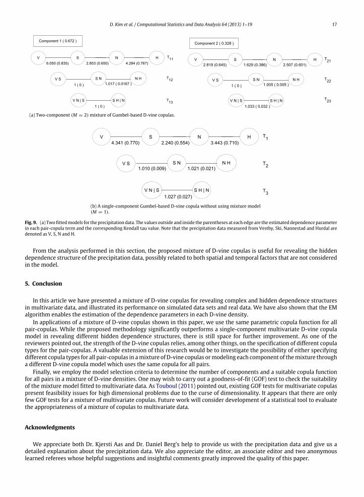
Fig. 9(a) shows the parameter estimation for a two-component mixture of Gumbel-based D-vine copulas in a treestructure. For the comparison purpose, Fig. 9(b) gives the estimates of the parameters for a single-component Gumbel-basedD-vine copula without using mixtures. We observe from Fig. 9(a) that the data consists of two components with differenttypes of dependence structures. The first component with 67.2% mixing proportion shows strong overall dependencebetween all four stations; the corresponding values of Kendall’s tau in the first level are 0.835 for Vestby, Ski, 0.650 forSki, Nannestad, and 0.767 for Nannestad, Hurdal in T11. This strong dependence structure may result from the fact thatall stations are located in the same county of Norway. The second component whose mixing proportion is 32.8%, on theother hand, describes a relatively weaker dependence pattern governed by the locality of the four stations. Note that theKendall’s tau value for Ski, Nannestad in the T21 is much smaller than the values for Vestby, Ski and Nannestad, Hurdalin the T21.
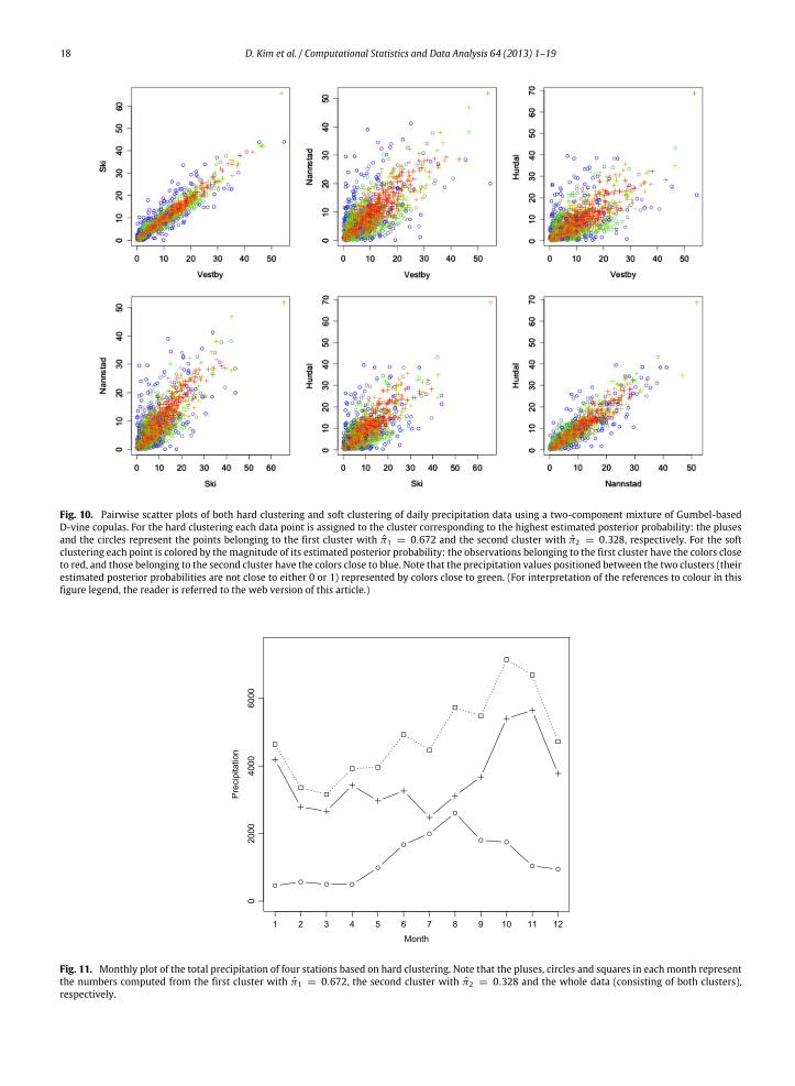
To further visualize the underlying structure of the precipitation data explained above, we construct the pairwise scatterplots of both hard and soft clustering of daily precipitation data using the posterior probability in Eq. (10) computed from thetwo-componentmixture ofGumbel-basedD-vine copulas (see Fig. 10). In eachpairwise plot the first clusterwith π1 = 0.672(points with plus symbols and colors close to red) consists of the precipitation values densely located near the 45 ° line. Onthe other hand, the second clusterwith π2 = 0.328 (points with circle symbols and colors close to blue) has values relativelyfar from the 45 ° line. Notice that the points for Vestby, Ski and Nannestad, Hurdal belonging to the second cluster arecloser to the 45 ° line, compared to those for the other pairs of stations in the second cluster.
In addition, we also check if the two clusters obtained from a mixture of Gumbel-based D-vine copulas correspond toparticular periods of time by investigating the total precipitation of four stations for each cluster with respect to time. Fig. 11shows the monthly plot of the total precipitation of four stations based on hard clustering. The pattern of the first cluster(represented by the pluses) appears to generally follow that of the whole data (represented by the squares) over the year,unlike that of the second cluster (represented by the circles). The contributions of the second cluster to the whole data arenon-negligible only during the months of June to October.
D. Kim et al. / Computational Statistics and Data Analysis 64 (2013) 1–19 17
(a) Two-component (M = 2) mixture of Gumbel-based D-vine copulas.
(b) A single-component Gumbel-based D-vine copula without using mixture model(M = 1).
Fig. 9. (a) Two fittedmodels for the precipitation data. The values outside and inside the parentheses at each edge are the estimated dependence parameterin each pair-copula term and the corresponding Kendall tau value. Note that the precipitation data measured from Vestby, Ski, Nannestad and Hurdal aredenoted as V, S, N and H.
From the analysis performed in this section, the proposed mixture of D-vine copulas is useful for revealing the hiddendependence structure of the precipitation data, possibly related to both spatial and temporal factors that are not consideredin the model.
5. Conclusion
In this article we have presented a mixture of D-vine copulas for revealing complex and hidden dependence structuresin multivariate data, and illustrated its performance on simulated data sets and real data. We have also shown that the EMalgorithm enables the estimation of the dependence parameters in each D-vine density.
In applications of a mixture of D-vine copulas shown in this paper, we use the same parametric copula function for allpair-copulas. While the proposed methodology significantly outperforms a single-component multivariate D-vine copulamodel in revealing different hidden dependence structures, there is still space for further improvement. As one of thereviewers pointed out, the strength of the D-vine copulas relies, among other things, on the specification of different copulatypes for the pair-copulas. A valuable extension of this research would be to investigate the possibility of either specifyingdifferent copula types for all pair-copulas in amixture of D-vine copulas ormodeling each component of themixture througha different D-vine copula model which uses the same copula for all pairs.
Finally, we employ the model selection criteria to determine the number of components and a suitable copula functionfor all pairs in a mixture of D-vine densities. One may wish to carry out a goodness-of-fit (GOF) test to check the suitabilityof the mixture model fitted to multivariate data. As Touboul (2011) pointed out, existing GOF tests for multivariate copulaspresent feasibility issues for high dimensional problems due to the curse of dimensionality. It appears that there are onlyfew GOF tests for a mixture of multivariate copulas. Future work will consider development of a statistical tool to evaluatethe appropriateness of a mixture of copulas to multivariate data.
Acknowledgments
We appreciate both Dr. Kjersti Aas and Dr. Daniel Berg’s help to provide us with the precipitation data and give us adetailed explanation about the precipitation data. We also appreciate the editor, an associate editor and two anonymouslearned referees whose helpful suggestions and insightful comments greatly improved the quality of this paper.
18 D. Kim et al. / Computational Statistics and Data Analysis 64 (2013) 1–19
Fig. 10. Pairwise scatter plots of both hard clustering and soft clustering of daily precipitation data using a two-component mixture of Gumbel-basedD-vine copulas. For the hard clustering each data point is assigned to the cluster corresponding to the highest estimated posterior probability: the plusesand the circles represent the points belonging to the first cluster with π1 = 0.672 and the second cluster with π2 = 0.328, respectively. For the softclustering each point is colored by themagnitude of its estimated posterior probability: the observations belonging to the first cluster have the colors closeto red, and those belonging to the second cluster have the colors close to blue. Note that the precipitation values positioned between the two clusters (theirestimated posterior probabilities are not close to either 0 or 1) represented by colors close to green. (For interpretation of the references to colour in thisfigure legend, the reader is referred to the web version of this article.)
Fig. 11. Monthly plot of the total precipitation of four stations based on hard clustering. Note that the pluses, circles and squares in each month representthe numbers computed from the first cluster with π1 = 0.672, the second cluster with π2 = 0.328 and the whole data (consisting of both clusters),respectively.
D. Kim et al. / Computational Statistics and Data Analysis 64 (2013) 1–19 19
References
Aas, K., Berg, D., 2009. Models for construction of multivariate dependence: a comparison study. The European Journal of Finance 15 (7), 639–659.Aas, K., Czado, C., Frigessi, A., Bakken, H., 2009. Pair-copula constructions of multiple dependence. Insurance: Mathematics & Economics 44 (2), 182–198.Akaike, H., 1973. Information theory and an extension of the maximum likelihood principle. In: Petrov, B.N., Csaki, F. (Eds.), 2nd International Symposium
on Information Theory. Akademiai Kiado, Budapest, pp. 267–281.Azzalini, A., Capitanio, A., 1999. Statistical applications of the multivariate skew normal distribution. Journal of the Royal Statistical Society Series B 61,
579–602.Azzalini, A., 2011. R package sn: The skew-normal and skew-t distributions (version 0.4-17). http://azzalini.stat.unipd.it/SN.Bauer, A., Czado, C., Klein, T., 2012. Pair-copula constructions for non-Gaussian DAG models. Canadian Journal of Statistics 40 (1), 86–109.Bedford, T., Cooke, R.M., 2001. Probability density decomposition for conditionally dependent random variables modeled by vines. Annals of Mathematics
and Artificial Intelligence 32, 245–268.Bedford, T., Cooke, R.M., 2002. Vines — a new graphical model for dependent random variables. Annals of Statistics 30 (4), 1031–1068.Brechmann, E., Czado, C., Aas, K., 2012. Truncated and simplified regular vines in high dimensions with application to financial data. Canadian Journal of
Statistics 40 (1), 68–85.Brechmann, E.C., Schepsmeier, U., 2011. Modeling dependence with C- and D-vine copulas: The R-package CDVine. R vignette of the R-package CDVine
(version 1.1-4).Bozdogan, H., 1987. Model selection and Akaikes information criterion (AIC): the general theory and its analytical extensions. Psychometrika 52 (3),
345–370.Carriére, J.F., 2006. Copulas, Encyclopedia of Actuarial Science.Celeux, G., Soromenho, G., 1996. An entropy criterion for assessing the number of clusters in a mixture model. Journal of Classification 13 (2), 195–212.Cherubini, U., Luciano, E., Vecchiato, W., 2004. Copula Methods in Finance. John Wiley, Chichester.Cuvelier, E., Noirhomme-Fraiture, M., 2005. Clayton copula and mixture decomposition, in: Janssen, J., Lenca, P., (Eds.), In: Applied Stochastic Models and
Data Analysis (ASMDA 2005), Brest, France, 17–20 May, pp. 699–708.Deheuvels, P., 1979. La fonction de dépendance empirique et ses propriétés: Un test nonparamétrique d’indépendence. Académie Royale de Belgique.
Bulletin de la Classe des Sciences. 5e Série 65, 274–292.Dempster, A.P., Laird, N.M, Rubin, D.B., 1977. Maximum likelihood from incomplete data via the EM algorithm. Journal of the Royal Statistical Society. Series
B 39 (1), 1–38.Efron, B., Tibshirani, R., 1993. An Introduction to the Bootstrap. Chapman & Hall, London.Genest, C., Ghoudi, K., Rivest, L.-P., 1995. A semi-parametric estimation procedure of dependence parameters in multivariate families of distributions.
Biometrika 82, 543–552.Genest, C., Quessy, J.-F., Rémillard, B., 2006. Goodness-of-fit procedures for copulamodels based on the probability integral transform. Scandinavian Journal
of Statistics 33 (2), 337–366.Genest, C., Rémillard, B., Beaudoin, D., 2009. Goodness-of-fit tests for copulas: a review and a power study. Insurance: Mathematics & Economics 44 (2),
199–213.Hobæk Haff, I., Aas, K., Frigessi, A., 2010. On the simplified pair-copula construction — simply useful or too simplistic? Journal of Multivariate Analysis 101
(5), 1296–1310.Hu, L., 2006. Dependence patterns across financial markets: a mixed copula approach. Applied Financial Economics 16 (10), 717–729.Joe, H., 1996. Families ofm-variate distributions with given margins andm(m − 1)/2 bivariate dependence parameters, in: Rüschendorf, L., Schweizer, B.,
Taylor, M. D., (Eds.), Distributions with fixed marginals and related topics, pp. 120–141.Joe, H., 1997. Multivariate Models and Dependence Concepts. Chapman & Hall, London.Joe, H., Li, H., Nikoloulopoulos, A.K., 2010. Tail dependence functions and vine copulas. Journal of Multivariate Analysis 101, 252–270.Kim, G., Silvapulle, M.J., Silvapulle, P., 2007. Comparison of semiparametric and parametric methods for estimating copulas. Computational Statistics &
Data Analysis 51 (6), 2836–2850.Kurowicka, D., Cooke, R.M., 2003. A parametrization of positive definite matrices in terms of partial correlation vines. Linear Algebra and its Applications
372, 225–251.Kurowicka, D., Cooke, R.M., 2004. Distribution — free continuous bayesian belief nets. in: Fourth International Conference on Mathematical Methods in
Reliability Methodology and Practice, Santa Fe, New Mexico.Kurowicka, D., Cooke, R.M., 2006. Uncertainty Analysis with High Dimensional Dependence Modelling. Wiley, New York.Lindsay, B.G., 1995. Mixture Models: Theory, Geometry and Applications. In: NSF-CBMS Regional Conference Series in Probability and Statistics, Vol. 5.
Institute of Mathematical Statistics and the American Statistical Association, Alexandria, Virginia.McLachlan, G.J., Peel, D., 2000. Finite Mixture Models. Wiley.McNeil, A.J., Frey, R., Embrechts, P., 2005. Quantitative Risk Management: Concepts, Techniques and Tools. Princeton University Press.Musshoff, O., Odening, M., Xu, W., 2006. Modeling and hedging rain risk. in: Annual Meeting of the American Agricultural Economics Association (AAEA),
Long Beach, USA, July pp. 23–26.Nelsen, R.B., 2006. An Introduction to Copulas, second ed. Springer, New York.Oakes, D., 1982. A model for association in bivariate survival data. Journal of the Royal Statistical Society. Series B 44 (3), 414–422.Oakes, D., 1994. Multivariate survival distributions. Journal of Nonparametric Statistics 3, 343–354.Onken, A., Grünewälder, S., Munk, M.H.J., Obermayer, K., 2009. Analyzing short-term noise dependencies of spike-counts in macaque prefrontal cortex
using copulas and the flashlight transformation. PLoS Computational Biology 5 (11), e1000577, 1–11.Panagiotelis, A., Czado, C., Joe, H., 2012. Pair copula constructions for multivariate discrete data. Journal of the American Statistical Association 107,
1063–1072.R Development Core Team, 2012. R: A Language and Environment for Statistical Computing. R Foundation for Statistical Computing, Vienna, Austria, ISBN:
3-900051-08-9, http://www.R-project.org.Rosenblatt, M., 1952. Remarks on a multivariate transformation. Annals of Mathematical Statistics 23 (3), 470–472.Schwarz, G., 1978. Estimating the dimension of a model. The Annals of Statistics 6 (2), 461–464.Schölzel, C., Friederichs, P., 2008. Multivariate non-normally distributed random variables in climate research — introduction to the copula approach.
Nonlinear Processes in Geophysics 15 (5), 761–772.Shih, J.H., Louis, T.A., 1995. Inference on the association parameter in copula models for bivariate survival data. Biometrics 51, 1384–1399.Sklar, A., 1959. Fonctions de répartition à n dimensions et leurs marges. Publications de l’Institut de Statistique de l’Université de Paris 8, 229–231.Smith,M.,Min, A., Almeida, C., Czado, C., 2010.Modelling longitudinal data using a pair-copula decomposition of serial dependence. Journal of the American
Statistical Association 105, 1467–1479.Touboul, J., 2011. Goodness-of-Fit Tests For Elliptical and Independent Copulas through Projection Pursuit. Algorithms 4 (2), 87–114.Vrac, M., Chédin, A., Diday, E., 2005. Clustering a Global Field of Atmospheric Profiles by Mixture Decomposition of Copulas. Journal of Atmospheric and
Oceanic Technology 22 (10), 1445–1459.Wu, C.F.J., 1983. On the convergence properties of the EM algorithm. The Annals of Statistics 11 (1), 95–103.