Mobile and Sensor Systems

Lecture 4: Sensor Network RoutingProf Cecilia Mascolo

In this lecture

• We will introduce sensor network routing protocols, in particular:– Directed diffusion– MINT routing

• We will talk about sensor network management and reprogramming

2

Network Protocols• Can we apply ad hoc networks protocols?• Yes protocols like epidemic can be applied but

overhead is an issue.• Aims are usually different: not communication but

data reporting to single or multiple source.• Specific protocols have been devised.• Specific nodes are interested in specific events:– Sink interested in all results;– Sink interested in a sensor reading change.

Protocols for Repeated interactions• Subscribe once, events happen multiple times:– Exploring the network topology might actually

pay off. But: unknown which node can provide data, multiple nodes might ask for data.! How to map this onto a “routing” problem?

• Put enough information into the network: publications and subscriptions can be mapped onto each other.But try to avoid using unique identifiers: might not be available, might require too big a state size in intermediate nodes.!

Directed Diffusion

• Directed diffusion as one option for implementation:– Try to rely only on local interactions.

–Data-centric approach.• Nodes send “interests” for data which are

diffused in the network.• Sensors produce data which is routed according

to interests.• Intermediate nodes can filter/aggregate data.

6

Directed Diffusion

EventSensorsources

Sensorsink

DirectedDiffusion

Asensor field

Interest Propagation• Each sink sends expression of

interests to neighbours.• Each node will store interests

and disseminate those further to their neighbours.– Cache of interest is checked

not to repeat disseminations.• Interests need refreshing from

the sink (they time out).• Interests have a “rate of events”

which is defined as “gradient”.

S

N

8

Interest Example

Type = Wheeled vehicle // detect vehicle locationInterval = 20 ms // send events every 20ms Duration = 10 s // Send for next 10 sField = [x1, y1, x2, y2] // from sensors in this area

Data delivery• Sensor data sources emit events which are sent

to neighbours according to interest (ie if there is a gradient).

• Each intermediate node sends back data at a rate which depends on the gradient.– ie if gradient is 1 event per second and 2

events per second are received send either the first or a combination of the two (aggregation).

Gradients Reinforcement• Events are stored to avoid cycles (check if same

event received before).• Data can reach a node through different paths.

Gradient reinforcement needed.

• When gradients are established the rate is defined provisionally (usually low). Sinks will ‘reinforce’ good paths which will be followed with higher rate.

• A path expires after a timeout so if not reinforced it will cease to exist. This allows adaptation to changes and failures.

Directed diffusion –Two-phase pull

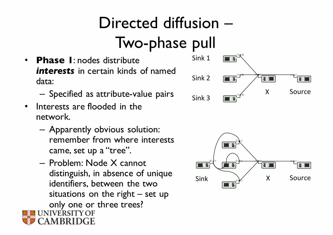
• Phase 1: nodes distribute interests in certain kinds of named data: – Specified as attribute-value pairs

• Interests are flooded in the network.– Apparently obvious solution:

remember from where interests came, set up a “tree”.

– Problem: Node X cannot distinguish, in absence of unique identifiers, between the two situations on the right – set up only one or three trees?

Sink1

Sink2

Sink3SourceX

Sink SourceX

Direction diffusion Gradients in two-phase pull

• Option 1: Node X forwarding received data to all “parents” in a “tree”: Not attractive, many needless packet repetitions over multiple routes.

• Option 2: node X only forwards to one parent. Not acceptable, data sinks might miss events.

• Option 3: Only provisionally send data to all parents, but ask data sinks to help in selecting which paths are redundant, which are needed.– Information from where an interest came is called

gradient.– Forward all published data along all existing gradients

13

Direction diffusion Gradients in two-phase pull

Event

SinkAsensor field

Reinforcedgradient

Reinforcedgradient

Directed diffusion –extensions

• Problem: Interests are flooded through the network.

• Geographic scoping & directed diffusion: Interest in data from specific areas should be sent to sources in specific geo locations only.

• Push diffusion – few senders, many receivers: Same interface/naming concept, but different routing protocol.Here: do not flood interests, but flood the (relatively few) data. Interested nodes will start reinforcing the gradients.

Issues• Purely theoretical work.• Apart from the flooding of the interests…No

consideration of real world issues such as link stability or link load and load dependence.

• Mac Layer issues (assume nodes are awake…or does not discuss it).

• More recent approaches have considered link capabilities more explicitly as part of the routing decision making.

Data aggregation

• Less packets transmitted -> less energy used

• To still transmit data, packets need to combine their data into fewer packets ! aggregation is needed

• Depending on network, aggregation can be useful or pointless • Directed diffusion gradient might require some data aggregation

Metrics for data aggregation

• Accuracy: Difference between value(s) the sink obtains from aggregated packets and from the actual value (obtained in case no aggregation/no faults occur)

• Completeness: Percentage of all readings included in computing the final aggregate at the sink

• Latency• Message overhead

Link quality based routing• Directed diffusion uses some sort of implicit ways

to indicate which are the good links.– Through the gradient.

• Ad hoc routing protocols for mobile networks route messages based on shorter path in terms of number of hops.

• The essence of the next protocol we present: “number of hops might not be the best performance indication in wireless sensor network”.

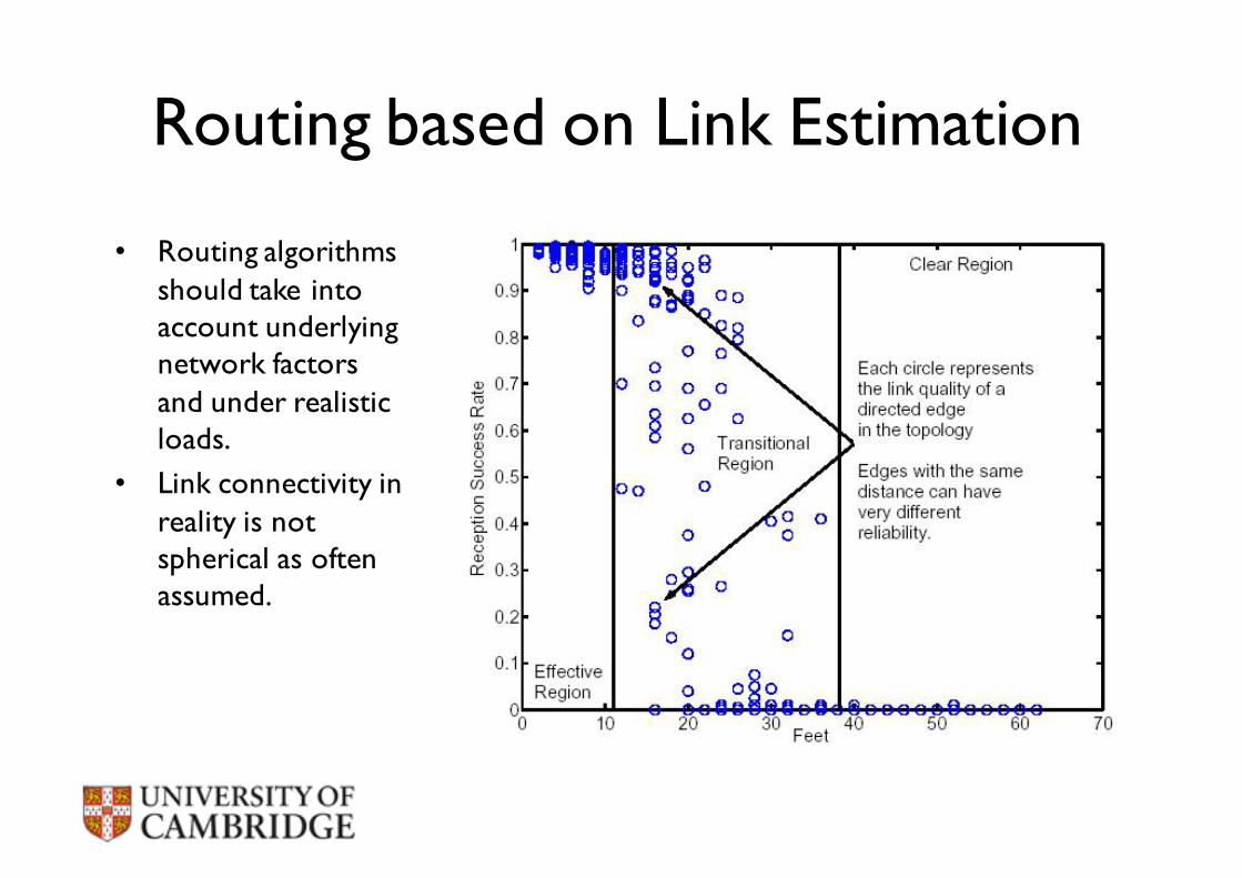
Routing based on Link Estimation

• Routing algorithms should take into account underlying network factors and under realistic loads.

• Link connectivity in reality is not spherical as often assumed.

20

RSSI – Stationary

June2008 WEIShortCourseL7-link 20

21

RSSI – Driving

June2008 WEIShortCourseL7-link 21

Link Estimation

• A good estimator in this setting must:– Be stable.– Be simple to compute and have a low memory

footprint.– React quickly to large changes in quality.

–Neighbour broadcast can be used to passively estimate.

WMEWMA• Snooping– Track the sequence numbers of the packets from

each source to infer losses• Window mean with EWMA– EWMA(tx)=a (MA(tx)) + (1-a)EWMA(t(x-1))– tx : last time interval; a: weight–MA(tx) is the number of packets received in the last

period.

WMEWA (t =30, a =0.6)

Neighborhood Management

• Neighborhood table:– Record information about nodes from which it

receives packets (also through snooping).• If network is dense, how does a node determine

which nodes it should keep in the table?• Keep a sufficient number of good neighbours in

the table.

Link Estimation based Routing

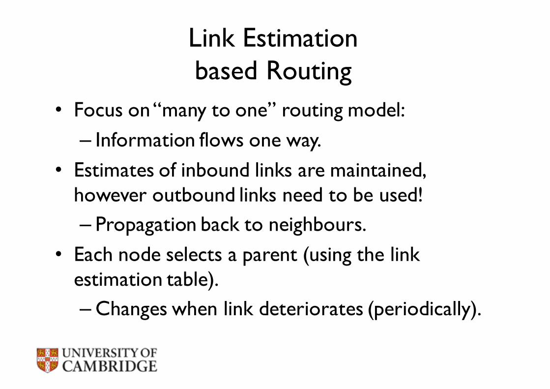
• Focus on “many to one” routing model:– Information flows one way.

• Estimates of inbound links are maintained, however outbound links need to be used!– Propagation back to neighbours.

• Each node selects a parent (using the link estimation table).–Changes when link deteriorates (periodically).

Distance vector routing: cost metrics

• Routing works as a standard distance vector routing.

• The DVR cost metric is usually the hop count.• In lossy networks hop count might underestimate

costs.– Retransmissions on bad links: shortest path

with bad links might be worse than longer path with good links.– Solution: consider the cost of retransmission

on the whole path.

MIN-T Route

• MT (Minimum Transmission) metric: – Expected number of transmissions along the

path.– For each link, MT cost is estimated by

1/(Forward link quality) * 1/(Backward link quality).• backward links are important for acks.

• Use DVR with the usual hop counts and MT weights on links.

An Example

S

D E

CBA

0.3

0.2

0.4

0.70.2

RoutingTableonD:Id Cost NextHopA 0.2 AB 0.7 BS 0.5 A

Sensor Network Programming/Reprogramming• Long Lifetime requires retasking the sensors.• However programming each node separately may

not be feasible.• What is reprogramming?– Send function parameters (“wake up every X

seconds”).– Sending binaries or code to compile.

• Checking that each node has the right code can be quite costly too.

30

Idea

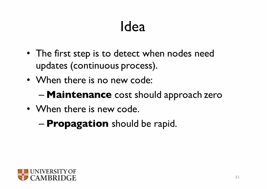
• The first step is to detect when nodes need updates (continuous process).

• When there is no new code:–Maintenance cost should approach zero

• When there is new code.–Propagation should be rapid.

31

Trickle

• Simple, “polite gossip” algorithm.

• “Every once in a while, broadcast what code you have, unless you’ve heard some other nodes broadcast the same thing, in which case, stay silent for a while.”

32

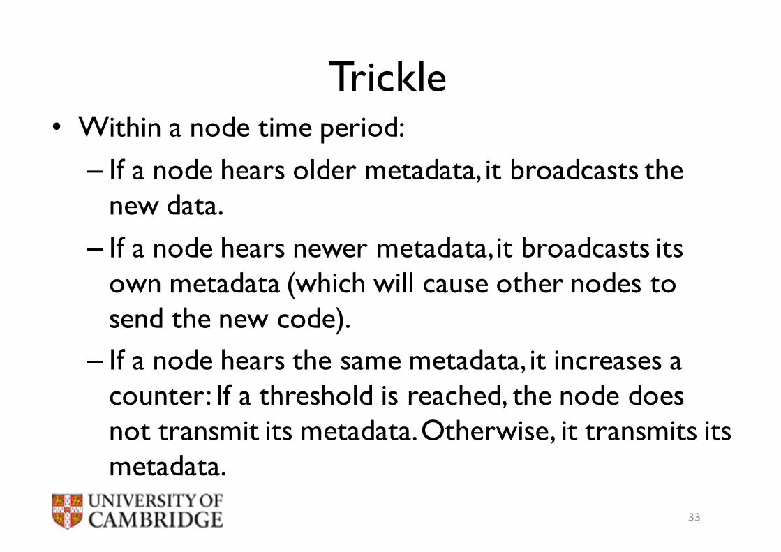
Trickle• Within a node time period:– If a node hears older metadata, it broadcasts the

new data.– If a node hears newer metadata, it broadcasts its

own metadata (which will cause other nodes to send the new code).

– If a node hears the same metadata, it increases a counter: If a threshold is reached, the node does not transmit its metadata.Otherwise, it transmits its metadata.

33

Trickle – Main Parameters

• Counter c: Count how many times identical metadata has been heard

• k: threshold to determine how many times identical metadata must be heard before suppressing transmission of a node’s metadata

• t: the time at which a node will transmit its metadata. t is in the range of [0, τ]

34

Example Trickle Execution

t1a t1b

time

t2a t2b

τt3a t3b

2

3

transmission suppressedtransmission reception

1

k=1c

1

0

1

35

Summary

• We have described sensor network challenges and solutions

• We have talked about sensor network management and reprogramming

36

References

• Intanagonwiwat, C., Govindan, R., and Estrin, D. 2000. Directed diffusion: a scalable and robust communication paradigm for sensor networks. In Proceedings of the 6th Annual international Conference on Mobile Computing and Networking (Boston, Massachusetts, United States, August 06 - 11, 2000). MobiCom '00. ACM, New York, NY, 56-67.

• Woo, A., Tong, T., and Culler, D. 2003. Taming the underlying challenges of reliable multihop routing in sensor networks. In Proceedings of the 1st international Conference on Embedded Networked Sensor Systems (Los Angeles, California, USA, November 05 - 07, 2003). SenSys '03. ACM, New York, NY. Pages: 14-27.

• Levis P., Patel L., Shenker S., Culler D. 2004. Trickle: A Self-Regulating Algorithm for Code Propagation and Maintenance in Wireless Sensor Networks. In Proceedings of the First USENIX/ACM Symposium on Networked Systems Design and Implementation (NSDI 2004). Pages 15-28.