mobility data mining - unipi.itdidawiki.cli.di.unipi.it/.../dm/chap06_mobility_data_mining-1.pdf ·...

1

Mobility data miningMirco Nannia

1.1 Introduction

1.1.1 What is mobility data mining

The trajectories of a moving object are a powerful summary for its ac-tivity related to mobility. As seen in previous chapters, such informationcan be queried in order to retrieve those trajectories (and the objectsthat own them) that respond to some given search criteria, for instancefollowing a predefined interesting behavior. However, when massive in-formation is available, we might be able to move a step forward and askthat such “interesting behaviors” automatically emerge from the data.That is precisely the domain explored by mobility data mining.

Moving from queries to data mining essentially consists in adding de-grees of freedom to the search process that the algorithms perform. Forinstance, a query might consist in searching those trajectories that atsome point perform the following sequence of maneuvers: abrupt slowdown, U-turn and finally accelerate. One possible corresponding datamining task, instead, might require to discover which sequences of ma-neuvers are performed frequently in the database of trajectories. Then,the output sequences obtained might contain also the slow-down → U-turn → accelerate example mentioned above. To perform this data min-ing process the user needs to specify the general structure of the behav-iors he/she searches (sequences), what kind of elements they can contain(the set of maneuvers to consider, as well as a precise way to locate agiven maneuver within a trajectory), and a criterion to select “inter-esting” behaviors – in our example, the user wants only behaviors thatappear frequently in the data.

a KDD Lab, ISTI-CNR, Pisa, Italy

2 Mobility data mining

1.1.2 Note on terminology

In this chapter we will make frequent use of the terms “trajectory pat-tern”. As mentioned in Chapter 1, the notion of trajectory pattern issubstantially equivalent to that of “trajectory behavior”, which also ap-peared in previous chapters of this book. The two notions originate fromdifferent communities and simply reflect different perspectives of thesame subject: the data management view (where “trajectory behavior”originates) focuses more on determining which trajectory is associated toeach behavior; the data mining view, on the contrary, is more focusedon what are the interesting behaviors in the input trajectories.

The several forms and variants of existing analysis tasks that belongto mobility data mining cannot be easily categorized into a set of fixedclasses. However, it is possible to recognize a few simple dimensionsalong which to locate the different analysis methods. In the following wemention one of them, that will be also used later as guideline during thepresentation of analysis examples.

1.1.3 Local patterns vs. global models

The example of behavior illustrated at the beginning of this section isrepresentative of a class of mining methods, called local patterns or, inmost contexts, simply patterns. The key point of local patterns is the aimof identifying behaviors and regularities that involve only a (potentiallysmall) subset of trajectories, and that describe only a (potentially small)part of each trajectory involved.

The complementary class of mining methods is called global models, orsimply models. Their objective is to provide a general characterizationof the whole dataset of trajectories, thus going towards the definitionof general laws that regulate the data, rather than spotting interestingyet isolated phenomena. For instance, we will see later mining tasksaimed to define a global subdivision of all trajectories into homogeneousgroups, as well as tasks aimed to discover rules able to predict the futureevolution of a trajectory (i.e., the next locations it will visit).

In the rest of the chapter we will provide an overview of the problemsand methods available in the mobility data mining field. For obviousreasons of space, the discussion will not cover exhaustively the availableliterature on the subject, and instead will propose some representativeexamples of the various topics. The presentation will mainly follow thedistinction between local patterns and global models introduced above.

1.2 Local trajectory patterns/behaviors 3

1.2 Local trajectory patterns/behaviors

The mobility data mining literature offers several examples of trajectorypatterns that can be discovered from trajectory data. Despite this widevariety, most proposals actually respect two basic rules: first, a pattern isinteresting (and therefore extracted) only if it is frequent, and thereforeit involves (or appears in) several trajectories1; second, a pattern mustdescribe the movement in space of the objects involved, and not onlyaspatial or highly abstracted spatial features.

While the spatial component of trajectory data is virtually always partof the patterns extracted, the temporal one (also intrinsic in trajectorydata) can be treated in several different ways, and we will use this differ-entiation to better organize the presentation. Then, while a trajectorypattern always describes a behavior that is followed by several movingobjects, we can choose whether they should do so together (i.e., duringthe period), at different moments yet with same timings (i.e., there canbe a time shift between the moving objects), or in any way, with noconstraints on time.

1.2.1 Using absolute time or Groups that move together

One of the basic questions that arise when analyzing moving objectstrajectories is the following:

Are there groups of objects that move together for some time?

For instance, in the realm of animal monitoring such kind of patternswould help to identify possible aggregations, such as herds or simplefamilies, as well as predator-prey relations. In human mobility, similarpatterns might indicate groups of people moving together on purposeor forced by external factors, e.g. a traffic jam, where cars are forced tostay close to each other for a long time period.

Obviously, the larger are the groups and/or the longer is the periodthey stay together, the higher is the likelihood that the observed phe-nomenon is significant and not a pure coincidence. For instance, if twomembers of a population of zebras under monitoring happen to move

1 While that holds for the majority of methods appeared in the mobility datamining literature, significant exceptions exist, including the extreme case ofoutliers detection, consisting of anomalous (and thus infrequent) patterns. Forease of presentation, outlier detection will be described later in this chapter, inthe context of global models.


close to each other for a short time, that can be seen as a random en-counter. However, if dozens of zebras are observed together for severalhours, we can safely assume that they form a herd or something is hap-pening that forces them to keep together.

The simplest form of trajectory pattern in literature that exactly an-swers the question posed above is the trajectory flock. As the name sug-gests, a flock is a group of moving objects that satisfy three constraints:

• a spatial proximity constraint: within the whole duration of the flock,all its members must be located within a disk of radius r – possiblya different one at each time instant, i.e. the disk moves to follow theflock;

• a minimum duration constraint: the flock duration must be at least ktime units;

• a frequency constraint: the flock must contain at least m members.

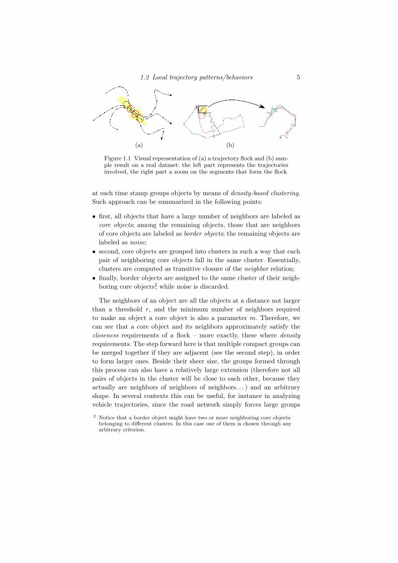
Figure 1.1(a) shows an abstract example of flock, where three trajecto-ries meet at some point (at the fifth time unit), keep close to each otherfor some time (four consecutive time units) and then separate (ninthtime unit). If, for instance, the constraints chosen by the user are theradius r used in the figure to draw the circles, a minimum duration offour time units (or less) and a minimum size of three members, then thecommon movement shown in the figure will be recognized as a flock.

Figure 1.1(b) shows an example extracted from a real dataset thatcontains GPS tracks of tourists in a recreational park (DwingelderveldNational Park, in Netherland). The leftmost section of the figure depictsthe three trajectories that were involved in the flock, while the rightmostone shows (a zoom with) only the segments of trajectories that createthe flock. As we can see, in this example a flock is a local pattern, bothin the sense of involving only a small subset of trajectories (three, in ourcase), and in the sense of describing an interesting yet relatively smallsegment of the whole life of the trajectories involved.

The general concepts of moving together or forming a group are imple-mented by the flocks framework in the simplest way possible: the objectsare required to be very close to each other during all the duration of theflock. However, a group might appear also under different conditions.One of these alternatives is to require that at each timestamp the objectsform a cluster – thus borrowing ideas and methods from the clusteringliterature. A notable example are moving clusters, a form of pattern that


(a) (b)

Figure 1.1 Visual representation of (a) a trajectory flock and (b) sam-ple result on a real dataset: the left part represents the trajectoriesinvolved, the right part a zoom on the segments that form the flock

at each time stamp groups objects by means of density-based clustering.Such approach can be summarized in the following points:

• first, all objects that have a large number of neighbors are labeled ascore objects; among the remaining objects, those that are neighborsof core objects are labeled as border objects; the remaining objects arelabeled as noise;

• second, core objects are grouped into clusters in such a way that eachpair of neighboring core objects fall in the same cluster. Essentially,clusters are computed as transitive closure of the neighbor relation;

• finally, border objects are assigned to the same cluster of their neigh-boring core objects2, while noise is discarded.

The neighbors of an object are all the objects at a distance not largerthan a threshold r, and the minimum number of neighbors requiredto make an object a core object is also a parameter m. Therefore, wecan see that a core object and its neighbors approximately satisfy thecloseness requirements of a flock – more exactly, these where densityrequirements. The step forward here is that multiple compact groups canbe merged together if they are adjacent (see the second step), in orderto form larger ones. Beside their sheer size, the groups formed throughthis process can also have a relatively large extension (therefore not allpairs of objects in the cluster will be close to each other, because theyactually are neighbors of neighbors of neighbors. . . ) and an arbitraryshape. In several contexts this can be useful, for instance in analyzingvehicle trajectories, since the road network simply forces large groups

2 Notice that a border object might have two or more neighboring core objectsbelonging to different clusters. In this case one of them is chosen through anyarbitrary criterion.


Figure 1.2 Visual example of a moving cluster over three time units

of cars to distribute along the roads (therefore creating a cluster withsnake-like shape) instead of freely agglomerate around a center (whichwould instead yield a compact, spherical-shape cluster).

A second, interesting feature that characterizes moving clusters is thefact that the population of objects involved in the pattern can gradu-ally change along the time: the only strict requirements are that at eachtimestamp a (spatial dense) cluster exists, and that when moving froma timestamp to the consecutive one the population shared by the corre-sponding spatial clusters is larger than a given fraction (a parameter ofthe method). A simple example of pattern that illustrates this point isshown in Figure 1.2: at each time slice a dense cluster is found, formedby three objects, and any pair of consecutive clusters share two overthree objects. This way, moving clusters that last a long time, mighteven start from a set of objects and end into a completely different (pos-sibly disjoint) set. In our example, only one object permanently belongsto the moving cluster. In some sense, the pattern is not strictly relatedto a population that generates it. The purpose of the pattern becomes todescribe phenomena that happen in the population, not to find a groupof individuals that do something peculiar consistently together.

One element of rigidity that affects both the patterns illustrated so faris the fact that they describe continuous portions of time. For instance, ifa herd that usually moves compactly gets dispersed for a short time (forinstance due to an attack by predators) and later gets compact again,both flocks and moving clusters will generally result into two differentand disconnected patterns – the before and the after the temporary dis-persion. One possible way to avoid this loss of information consists inallowing gaps in the patterns, i.e., a pattern involves a set of timestampsthat are not necessarily consecutive. In the literature we can find a solu-tion of this kind, known as swarm patterns. Swarms are a general formof patterns that generalize flocks and moving clusters, since any spa-tial clustering method can be applied at the level of single timestamp,


and then spatial clusters belonging to different timestamps are linked(in case they share an appropriate fraction of population) regardless oftheir temporal distance.

1.2.2 Using relative time

In some contexts, the moving objects we are examining might act in asimilar way, even if they are not together. For instance, similar dailyroutines might lead several individuals to drive their car along the sameroutes, even if they leave home at very different hours of the day. Or,tourists that visit a city in different days of the year might actually visitit in the same way – for instance by visiting the same places in the sameorder and spending approximately the same amount of time on them –because they simply share interests and attitude. This leads to a newcategory of questions, which can be well represented by the following:

Are there groups of objects that perform a sequence of movements, withsimilar timings though possibly during completely different moments?

Patterns like flocks and moving clusters can provide some answers tothe question, but usually it is a small set, since it is limited to movementsthat happen synchronously among all objects involved. The questionposed above involves a much weaker constraint on the temporal dimen-sion of the problem, and therefore might allow many more answers. Inthe following we will present one example of pattern that goes in thisdirection and extracts spatio-temporal behaviors that are followed byseveral objects, but allowing any arbitrary time shift between them.

T-Patterns (abbreviation of Trajectory patterns) are defined as se-quences of spatial locations with typical transition times, such as thefollowing two:

Railway Station15min−→ Museum2h15min−→ Castle Square

Railway Station10min−→ Middle Bridge10min−→ Campus

For instance, the first pattern might represent the typical behavior oftourists that rapidly reach a museum from the railway station and spendthere about two hours before getting to the adjacent square. The secondpattern, instead, might be related to students that reach the universitycampus from the station by passing through the mandatory passage onthe central bridge over the river. A graphical example is also providedin Figure 1.3(left).


The two key points that characterize T-patterns are the following:first, they do not specify any particular route among two consecutiveregions described: instead, a typical travel time is specified, which ap-proximates the (similar) travel time of each individual trajectory rep-resented by the pattern. In the gap between two consecutive regions atrajectory might even have stopped in other regions not described in thepattern; second, the individual trajectories aggregated in a pattern neednot to be simultaneous, since the only requirement to join the pattern isto visit the same sequence of places with similar transition times, evenif they start at different absolute times.

T-patterns are parametric on three main parameters: the set of spatialregions to be used to form patterns, i.e., the spatial extension of “Rail-way Station” and any other place considered relevant for the analysis3;the minimum support threshold, corresponding to the minimum size ofthe population that contributes to form the pattern (the parameter mfor flocks); and a time tolerance threshold τ , that determines the waytransition times are aggregated: transition times that differ less thanτ will be considered compatible, and therefore can be joined to form acommon typical transition time.

Figure 1.3(right) depicts an example of T-pattern on vehicle data de-scribing the movements of a fleet of trucks. The pattern shows that thereexists a consistent flow of vehicles from region A to region B, and thenback to region C, close to the origin. Also, the time taken to move fromregion A to region B (t1 in the figure) is around ten times larger thenthe transition time from B to C. That might suggest, for instance, thatthe first part of the pattern describes a set of deliveries performed bythe trucks, while the second part describes the fast return to the base.

1.2.3 Not using time

In many cases it is interesting to understand if there are typical routesfollowed by significant portions of the population, i.e.:

Are there groups of objects that perform a common route (or segmentof route), regardless of when and how fast they move?

That means, for instance, that we are interested in what path anindividual follows, but not the hour of the day he/she does it, nor the3 Actually, the algorithmic tool provided in literature to extract T-patterns also

contains heuristics to automatically define such regions, but in general thedomain expert might want to do it maually in order to better exploit itsknowledge or to better focus the analysis, or both.

1.3 Global trajectory models 9

Figure 1.3 Visual representation of a T-pattern (left) and sampleresult on a real dataset (right)

transportation means adopted: cars, bicycles, pedestrians and peopleon the bus might follow the same path yet at very different speeds,resulting in different relative times. Also notice that we are interestedhere in routes that might be just a small part of a longer trip of theindividual.

The mobility data mining literature provides a few definitions of pat-terns that can answer to the question given above. In particular, we willbriefly summarize one of the earliest proposals appeared, at that timenamed generically as spatio-temporal sequential pattern (in contrast, thetrend in recent times is to assign elaborate and sonorous names to anynew form of pattern or model).

The basic idea, also depicted in Figure 1.4, consists of two steps4:first, segments of trajectories are grouped based on their distance anddirection, in such a way that each group is well described by a single rep-resentative segment (see the two thick segments in the figure); second,consecutive segments are joined to form the pattern. Frequent sequencesare then outputted as sequences of rectangles such that their width quan-tifies the average distance between each segment and the points in thetrajectory it covers. Figure 1.4 depicts a simple pattern of this kind,formed of two segments and corresponding rectangles. In particular, itis possible to see how the second part of the pattern is tighter than thefirst one, i.e., the trajectory segments it represents are more compact.

1.3 Global trajectory models

A common need in data analysis at large is to understand which are thelaws and rules that drive the behavior of the objects under monitoring.4 The original proposal of this pattern considers a single, long input trajectory.

However, the same concepts can be easily extended to multiple trajectories.


Figure 1.4 Visual representation of a spatio-temporal sequential pat-tern

In the context of mobility data mining we refer to such laws and rulesas (global) trajectory models, and in this area we can recognize threeimportant representative classes of problems: dividing trajectories intohomogeneous groups; learning rules to label any arbitrary trajectorywith some tag, to be chosen among a set of predefined classes; predictingwhere an arbitrary trajectory will move next. In the following we willintroduce and discuss each of them.

1.3.1 Trajectory clustering

In data mining, clustering is defined as the task of creating groups ofobjects that are similar to each other, while keeping separated thosethat are much different. In most cases, the final result of clustering isa partitioning of the input objects into groups, called clusters, whichmeans that all objects are assigned to a cluster, and clusters are mutuallydisjoint. However, exceptions to this general definition exists and arerelatively common.

While the data mining literature is extremely rich of clustering meth-ods for simple data types, such as numerical vectors or tuples of a rela-tional database, moving to the realm of trajectory makes it difficult todirectly apply them. The problem is, trajectories are complex objects,and many traditional clustering methods are tightly bound to the simpleand standard data type they were developed for. In most cases, to usethem we need to adapt the existing methods or even to re-implementtheir basic ideas in a completely new, trajectory-oriented way. We willsee next some solutions that try to reuse as much as possible existingmethods and frameworks; then, we will discuss a few clustering methodsthat were tailored around trajectory data since the beginning.

Generic methods with trajectory distances. Several clustering methods


in the data mining literature are actually clustering schemata that can beapplied to any data type, provided that a notion of similarity or distancebetween objects is given. For this reason, they are commonly referred toas distance-based methods. The key point is that such methods do notlook at the inner structure of data, and simply try to create groups thatexhibit small distances between its members. All the knowledge aboutthe structure of the data and their semantics is encapsulated in thedistance function provided, which summarizes this knowledge throughsingle numerical values – the distances between pairs of objects; the algo-rithm itself, then, combines such summaries to form groups by followingsome specific strategy.

To give an idea of the range of alternative clustering schemata avail-able in literature, we mentioned three very common ones: k-means, hi-erarchical clustering, density-based clustering.

K-means tries to partition all input objects into k clusters, where k isa parameter given by the user. The method starts from a random par-titioning and then performs several iterations to progressively refine it.During an iteration, k-means first computes a centroid for each cluster,i.e., a representative object that lies in the perfect center of the clus-ter5), then re-assigns each object to the centroid that is closest to it.Such iterative process stops when convergence (perfect or approximate)is reached.

Hierarchical clustering methods try to organize objects in a multi-level structure of clusters and sub-clusters. The idea is that under tightproximity requirements, several small and specific clusters might be ob-tained, while loosening the requirements some clusters might be mergedtogether into larger and more general ones. For instance, agglomerativemethods start from a set of extremely small clusters – one singleton foreach input object – and iteratively selects and merge together the pairof clusters that are most similar. At each iteration, then, the number ofclusters decreases of one unit, and the process ends when only one hugecluster is obtained, containing all objects. The final output will be a datastructure called dendogram, represented as a tree where each singletoncluster is a leaf, and each cluster is a node having as children the twosub-clusters that originated it through merging.

Finally, density-based clustering, as already introduced in Section 1.2.1,

5 Notice that such object is a new one, computed from those in the cluster.Therefore, some level of understanding of the data structure is needed, here.When that is not possible, usually a variant is applied, called k-medoid thatselects the most central object of the cluster as representative.


is aimed to form maximal, crowded (i.e., dense) groups of objects, thusnot limiting the cluster extension or its shape and, in some cases, puttingtogether also couples of very dissimilar objects.

How to choose the appropriate clustering method? While no strictrule can exist, a general hint consists in paying attention to some ba-sic characteristics of the data and the expected characteristics of theoutput. For instance, if we expect that our data should form compactclusters of spherical shapes (i.e., they should agglomerate around somecenters of attraction), then k-means is a good candidate, especially if thedataset is large – k-means is known to be very efficient. However, theuser should know the number k of clusters to be found in the data, or atleast some reasonable guess. That can be avoided with hierarchical, ag-glomerative algorithms, since the dendograms they produce synthesizethe results that can be obtained for all possible values of k, from 1 to N(the number of input objects). The choice of the most appealing k can bepostponed after the computation, and be supported by an examinationof the dendogram. However, hierarchical clustering is usually expensive(efficient variants exist, yet introducing other factors to be evaluated), soit is not a good option with large datasets. Finally, density-based meth-ods apparently do not suffer of any of the issues mentioned above, andare also more robust to noisy data, yet the resulting clusters will usuallyhave an arbitrary shape and size – a feature that might be unacceptablein some contexts, and extremely useful in others.

Depending on the analysis task that the user wants to perform, oncethe clustering schema to be adopted has been selected, he/she needsto choose the most appropriate similarity function, i.e., the numericalmeasure that quantifies how much two trajectories look similar. Therange of possible choices is virtually unlimited. The examples that canbe found in the literature include the following, approximately sorted inincreasing order of complexity:

• spatial starts, ends, or both: two trajectories are compared based onlyon their starting points (the origin of the trip), or the ending point(the final destination of the trip), or a combination of them. Thedistance between the trajectories, then, reduces to the spatial distancebetween two points. When both starts and ends are considered, thesum or average of their respective distances is computed. The outputof a clustering based on these distances will generally put together


Figure 1.5 Sample trajectory clustering on a real dataset, obtainedusing a density-based clustering schema, and a spatial route distancefunction

trajectories that start or end in similar places, regardless of whenthey do start/end and what happens in the rest of the trajectory;

• spatial route: in this case, the spatial shape of the trajectory is consid-ered, and two trajectories that follow a similar path (though possiblyat different times and with different speeds) from start to end, willresult in a low distance.

• spatio-temporal route: in this case, also the time is considered, there-fore two trajectories will be similar when they approximately movetogether throughout their life.

Obviously, the selection of the clustering schema and the selectionof the distance function might also be performed in the opposite order.Indeed, in some cases the choice of the distance to adopt is relatively easyor even enforced by the specific application, in which case the selectionof the distance is performed first.

Figure 1.5(right) shows an example of result obtained by a specificcombination of schema and distance, namely a density-based clusteringalgorithm using the spatial route distance described above. Differentclusters are plotted with different colors. The dataset used in the examplecontains trajectories of vehicles in Tuscany, Italy, also plotted on the leftof the figure.

Trajectory-oriented clustering methods. A complementary approachto clustering, as opposed to the distance-based solutions described sofar, consists in algorithms that try to better exploit the nature andinner structure of trajectory data. From a technical point of view, that


usually translates to deeply re-adapt some existing solution in order toaccommodate the characteristics of trajectory data.

One important family of solutions makes use of standard probabilisticmodeling tools. A very early example was provided by mixture models-based clustering of trajectories. The basic idea is not dissimilar fromk-means: we assume that the data actually forms a set of k groups, andeach group can be summarized by means of a representative object. Thedifference is that now the representative is a probability distribution oftrajectories that fits well with the trajectories in its cluster. The keypoint in this approach, obviously, is exactly how a probability distribu-tion of trajectories can be defined (and fitted on a dataset). In short,the solution adopted computes a central representative trajectory plus arandom Gaussian noise around it. The closeness of a trajectory from thecluster center, then, is simply computed as its likelihood, i.e., the prob-ability that it was generated from the central trajectory adding someGaussian noise. Another well-known statistical tool often adopted whendealing with trajectories are Hidden Markov Models (HMMs). The basicapproach, here, consists in modeling a trajectory as a sequence of transi-tions between spatial areas. Then, a cluster of trajectories is modeled bymeans of a Markov model (i.e. the set of transition probabilities betweenall possible pairs of regions) that better fits the trajectories. Moreover,the precise position that a trajectory is expected to occupy within eachspatial region is also modeled through a probability distribution. Theclustering problem, then, consists in finding a set of HMMs (the clus-ters), such that each of them fits well with a subset of the trajectories.

Other examples of trajectory-oriented clustering methods can arise byadding novel dimensions to the clustering problem. For instance, in theliterature it was investigated the problem of finding clusters by means ofa distance-based clustering method (a density-based one, more exactly,though a similar process might be easily replicated for other approaches)when it is not known in advance the time interval to consider for clus-tering. For instance, we might expect that rush hours in urban trafficdata exhibit cluster structures that are better defined than what hap-pens in random periods of the day. The problem, then, becomes to findboth the optimal time interval (rush hours were just a guess to be con-firmed) and the corresponding optimal cluster structure. The solutionproposed, named time-focused trajectory clustering, adopts a trajectorydistance computed as the average spatial distance between the trajecto-ries within a given time interval, which is a parameter of the distance.Then, for each time interval T , the algorithm can be run focusing on the


Figure 1.6 Three-dimensional depiction of sample result obtainedwith time-focused trajectory clustering on a dataset of synthetic tra-jectories.

trajectory segments laying within T . The quality of the resulting clustersis evaluated in terms of their density, and an heuristics is provided toexplore only a reasonable subset of the possible values of T . A sampleresult of the process is given in Figure 1.6, that depicts a set of trajec-tories forming three clusters (plus some noise) and shows the optimaltime interval (that where the clusters are clearest) as dark trajectorysegments.

1.3.2 Trajectory classification

Clustering is also known as unsupervised classification, since the ob-jective is to find a way to put objects into groups without any priorknowledge of which groups might exist, and what their objects look like.In several contexts such knowledge is available, more exactly in the formof a set of predefined classes and a set of objects that are already labeledwith the class they belong to – the so called training set. The problem,here, becomes to find rules to classify new objects in a way that is co-herent with the prior knowledge, i.e. they fit well with the training set.For instance, we might have access to a set of vehicle trajectories thatwere manually labeled with the vehicle type (car, truck, motorbike), andwe would like to find a way to automatically label an other, much largerset of new trajectories.


The simplest solution to the problem is the so called k-nearest neigh-bors (kNN) approach: instead of inferring any classification rule, it di-rectly compares each new trajectory t against the training set, and findsthe k labeled trajectories that are closest to t. The most popular labelamong the neighbors is then assigned also to t. The assumption is thatthe more similar are two trajectories, the more likely they belong tothe same class. Obviously, everything revolves around a proper choicefor the similarity measure applied, which should be as much coherentas possible with the classification problem at hand. As an example, wecan expect that a similarity function which takes into consideration theacceleration of objects will recognize well the vehicle type – the lighterthe vehicle, the easier is to reach high accelerations. On the contrary, ameasure based only on the places visited might perform worse.

The same idea is also applied in several sampling-based solutions tothe clustering problem: when the dataset is too large to process, one ap-proach consists in randomly sampling a small subset of trajectories, andcomputing clusters on them. Then, all others trajectories are assigned tothe cluster (i.e., classified) with a kNN approach or by comparing themagainst the centroid of each cluster.

Approaching the problem from a different viewpoint, each class in-volved in the classification problem could be modeled through a prob-abilistic model that is fitted to the available trajectories in the class.Then, each new trajectory can be assigned to the class whose modelmost likely generated it. Similarly to what we have seen with clustering,hidden Markov models are a common choice to do it. As compared toclustering, the problem is now simplified, since the association trajecto-ries↔ classes is known apriori. Behind the probabilistic framework theyoperate in, HMMs essentially aggregate trajectories based on their over-all shape, again assuming that similar trajectories have better chancesof belonging to the same class.

The final way to classify trajectories we will see, is based on a tradi-tional two-steps approach: first extract a set of discriminative featuresby a preliminary analysis of the trajectories; then, use such features –that can be expressed as a database tuple or a vector – to train anyexistent standard classification model for vector/relational data.

The first step requires to understand which characteristics of the tra-jectories appear to better predict which class each trajectory belongs to.One straightforward approach might consist in calculating a predefinedset of measures expected to be informative enough for the task. For in-


stance, aggregates such as average speed of the trajectory, its length,duration, average acceleration and diameter of the covered region mightbe used. Other, more sophisticated, solutions might instead try to ex-tract finer aspects of the movement, tuned to calculate only the mostuseful ones. A proposal of this kind can be find in literature with thename TraClass, which heavily relies on a trajectory clustering step.

TraClass is based on a fundamental observation: in several (if notmost) cases, the features that best discriminate trajectory classes arerelated to a small part of the overall trajectory. All approaches men-tioned so far, on the contrary, uniquely consider overall characteristics– that includes HMM-based solutions, since each model must fit wholetrajectories. Single, short-duration events hidden in the long life of atrajectory might then be lost in the process. TraClass tries to fill in thegap by extracting a set of trajectory behaviors (which, we recall, lookfor local behaviors rather than overall descriptions of full trajectories).The basic tool adopted is trajectory segmentation and the clustering ofsuch segments to form movement patterns.

TraClass works at two levels: regions and trajectory segments. At thefirst one, it extracts higher-level features based on the regions of spacethat trajectories visited, without using movement patterns; at the secondone, lower-level trajectory-based features are computed, using movementpatterns. The extraction phase is made more effective by evaluating thediscriminative power of the regions and patterns under construction. Forinstance, a frequent movement that is performed by trajectories of allclasses will be not useful for classification (knowing that a trajectory con-tains such pattern does not help in guessing the right class to associateto it); on the contrary, a slightly less frequent pattern that is mostly fol-lowed by trajectories of a single class is a very promising feature. In theproposed framework, trajectory partitioning makes discriminative partsof trajectories identifiable, and the two types of patterns collaborate tobetter characterize trajectories.

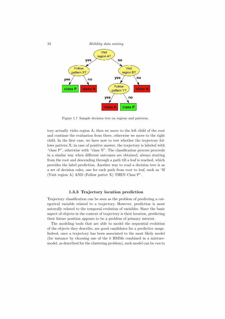
Once a vector of features has been computed for each trajectory, wecan choose any generic, vector-based classification algorithm. One rep-resentative (and easy to grasp) example are decision trees. The resultingclassification model has the structure of a tree, whose internal nodesrepresent tests on the features of the object to classify, and the leavesindicate the class to associate to the objects. Figure 1.7 shows a fictitiousexample based on TraClass features, with two classes: positive (P) andnegative (N). When a new trajectory needs to be classified, the test onthe root (the top circle) is performed on it. In the example, if the trajec-


Figure 1.7 Sample decision tree on regions and patterns.

tory actually visits region A, then we move to the left child of the rootand continue the evaluation from there, otherwise we move to the rightchild. In the first case, we have now to test whether the trajectory fol-lows pattern X: in case of positive answer, the trajectory is labeled with“class P”, otherwise with “class N”. The classification process proceedsin a similar way when different outcomes are obtained, always startingfrom the root and descending through a path till a leaf is reached, whichprovides the label prediction. Another way to read a decision tree is asa set of decision rules, one for each path from root to leaf, such as “If(Visit region A) AND (Follow patter X) THEN Class P”.

1.3.3 Trajectory location prediction

Trajectory classification can be seen as the problem of predicting a cat-egorical variable related to a trajectory. However, prediction is mostnaturally related to the temporal evolution of variables. Since the basicaspect of objects in the context of trajectory is their location, predictingtheir future position appears to be a problem of primary interest.

The modeling tools that are able to model the sequential evolutionof the objects they describe, are good candidates for a predictive usage.Indeed, once a trajectory has been associated to the most likely model(for instance by choosing one of the k HMMs combined in a mixture-model, as described for the clustering problem), such model can be run to


Figure 1.8 Sample Prediction tree produced by WhereNext.

simulate the most likely next steps. In most cases we can apply the sameremarks discussed earlier in this section for classification: if the modelis based on an overall summary of the behavior of a set of trajectories,most likely it will not be able to capture local events, even though theirappearance is highly correlated with a future behavior – in our case, thenext location.

In literature it can be found an approach called WhereNext, that worksin a way not too dissimilar from the one followed by TraClass for the clas-sification problem. Basically, WhereNext extracts T-patterns (see Sec-tion 1.2.2) from a training dataset of trajectories and combine them intoa tree structure similar to a prefix-tree. In particular, each root-to-nodepath corresponds to a T-pattern, and root-to-leaf paths correspond tomaximal patterns. Figure 1.8 shows a sample prediction tree, condensing12 patterns, 7 of which are maximal (one per leaf).

When a new trajectory is presented, its most recent segment is com-pared against the regions represented in the tree, looking for the bestmatch among the root-to-node paths. For instance, Figure 1.8 depictsthe case where the last part of the trajectory visits region A followedby region B after a delay between 9 and 15 time units. The match isdepicted by the red sequence. Then, the model finds that the matchedsequence is a prefix of a longer pattern, and so it suggests as likely con-tinuation region E (marked in green in the figure), to be reached after adelay between 10 and 56 time units.

WhereNext has a few characteristic features that distinguish it frommost alternative approaches: first, the next location prediction is equippedalso with a temporal delay; second, if no good match is found between


new trajectories and prediction tree, no prediction is provided, whilemost standard approaches always output a suggestion, even if it has anextremely low confidence; finally, the location prediction occurs in termsof regions and not single spatial points, although the center of the regioncan be returned if a single point is required by the specific application.

1.3.4 Trajectory outliers

The general objective of clustering is to fit each object in data intosome category (and discovering the categories is part of the problem).However, sometimes the analyst is exactly interested in those objectsthat deviate from the rest of the dataset, and therefore cannot really fitany category. Such objects are called outliers.

Finding an outlier object means to discover some feature or patternthat holds for the object, and yet is anomalous or at least very rarein the dataset. In this sense, the problem can be properly seen as a(infrequent) pattern discovery task. The reason for discussing it now isthat most outlier detection methods in literature actually adopt someclustering procedure, and identify outliers as those objects that are (orwould be) left out of any cluster. Here we provide two examples.

A basic method for discovering trajectory outliers consists in adopt-ing a density-based clustering perspective, and therefore compute thenumber of neighbors of each trajectory over a reasonably large neigh-borhood. Then, the trajectories that have too few neighbors are classifiedas outliers. As density-based clustering, the method is parametric on thedistance measure adopted, and therefore, in principle, any distance be-tween trajectories can be applied. Alternatively, from each trajectory aset of predefined representative features can be extracted, such as av-erage speed, initial position, and similar, and then apply any standarddistance over vector data.

In Section 1.3.2 the TraClass trajectory classification method was pre-sented, which has the characteristic of working over trajectory segments(obtained by properly cutting original trajectories) rather than wholetrajectories. By clustering such segments, relevant sub-trajectory pat-terns were extracted and later used for classification purposes. Followingthe same idea, outliers can be found within trajectory segments, there-fore focusing on single parts of trajectory that behave in a anomalousway. In particular, each trajectory segment is compared against the rep-

1.4 Conclusion 21

resentative segment of each cluster, and if no representative segment fitswell enough, the input trajectory segment is classified as outlier.

1.4 Conclusion

We conclude this chapter with a few notes on the topics presented andsome of the open questions in mobility data mining research.

1.4.1 Summary

Mobility data mining, as many other instantiations of the general datamining paradigm into specific contexts, brings with itself the generalcategorization of problems and methods it inherited from standard datamining. In particular, the three main categories – frequent patterns,clustering and classification – appear again. However, some specifici-ties of trajectory data emerged and stimulated the development of newapproaches. In particular, the complexity of the data, joining temporaland spatial information, greatly increases the search space of most inter-esting problems, such as finding patterns or discovering discriminativespatio-temporal features for classification or prediction problems.

1.4.2 Open questions

One aspect of mobility data mining that the reader might have guessedby reading this chapter is the fact that it still lacks an overall, compre-hensive and clear theoretical framework. Such a framework should beable to accommodate existing problems and solutions proposed in liter-ature, as well as clarify the relations between them. Some examples ofefforts in this direction exist in literature, and we also reported a few ofthem – for instance, the relation between local trajectory patterns andglobal trajectory classification models, and their ability to grasp differ-ent, complementary kinds of discriminatory features of trajectory data;or the relations between some of the various forms of trajectory pattern.However, such cases are rather isolated, and at the present, providing anintegrated view of methods and issues is still a largely unexplored partof the research field.

Another important point in mobility data mining is the fact that sev-eral data sources might provide information about the same mobilityphenomena coming from different viewpoints. Each data source usually


has distinctive characteristics, strong points and limitations, and theirintegration might help in overcoming the limits of each of them. For in-stance, vehicle GPS data are usually very detailed in space (i.e., spatialuncertainty is small) and time (frequency of data acquisition is rela-tively high), yet it is inherently limited to the vehicles that are involvedin the data collection process; instead, mobile phone service providersare able to collect information about mobility of all their customers, andthrough the collaboration of a few providers it is possible to cover theactivity of very large portions of the real population. One example arecall detail records (CDRs), that describe the cell towers that served eachcall performed by each phone, together with its timestamp. CDRs allowto build mobility trajectories for each customer served. However, suchtrajectories are very sparse (one point corresponds to a call, which areusually not so frequent) and spatially rough (a point actually representsthe whole area served by the cell tower). Activities that try to com-bine these two data sources are appearing nowadays, with the aim ofimproving the representativity of GPS data through the extremely highpenetration of the (spatially and temporally poor) CDR data.

Finally, so far, our discussion has always implicitly assumed that thetrajectory data were analyzed off-line and in a centralized setting, i.e.,by first collecting all data in a single database and then analyzing them.However, mobility data are usually massive and arrive as a continuousstream from the data source(s). Massiveness and streaming nature ofdata leads, at a large scale, to make it impossible to collect them in acentralized database, and therefore analysis methods need to be devel-oped that exploit appropriate technologies, such as distributed databases(a paradigm where data are distributed along several data centers, to bequeried to obtain the data needed for each specific analysis or compu-tation step), distributed computation (several nodes with computationpowers collaborate to analyze data) and streaming-oriented computa-tion (essentially aimed to perform computation by looking at the inputdata only once).

1.5 Bibliographic Notes

As mentioned at the beginning of the chapter, the literature on mobilitydata mining is rather extensive – especially for such a young field – andheterogeneous. Attempting an exhaustive discussion of existing problemsand proposals would require much more space and would be beyond our

1.5 Bibliographic Notes 23

purposes as well. In the following, we will provide an essential list ofbibliographic references for the reader, including those describing themethods cited in the chapter and a few pointers for further readings.

The original definition of flock patterns required that the group ofobjects meet at a single time instant and have the same direction ofmovement. Successive variants introduced the temporal duration con-straint, also adopted in this chapter, starting from Gudmundsson et al.(2004). Moving clusters were defined by Kalnis et al. (2005), providedwith a few heuristics for incrementally computing the interesting pat-terns, while spatio-temporal sequential patterns appeared in Cao et al.(2005).

T-patterns were introduced by Giannotti et al. (2007), and later wereexploited in building WhereNext – a location prediction method by Mon-reale et al. (2009) – as well as in several application works.

One rich source for a library of trajecory distances – to be used withingeneric clustering algorithms – is provided by Pelekis et al. (2007). Sev-eral references exist for standard (distance-based) clustering schema thatcan be applied to trajectory data, including basic introductions to datamining such as Tan et al. (2005).

Model-based approaches to trajectory clustering can be found in sev-eral, isolated papers, especially on specific application domains (videosurveillance, animal tracking, etc.). The mixture-models trajectory clus-tering described in this chapter was first introduced in Gaffney andSmyth (1999), later extended to include time shifts. Hidden MarkovModels-based approaches can be found, for instance, in Mlich and Chme-lar (2008).

Time-focused clustering, an extension of density-based clustering fortrajectories, was presented in Nanni and Pedreschi (2006).

The TraClass framework for trajectory classification was introduced inLee et al. (2008a), mainly based on previous works of the same authorson trajectory segmentation and clustering. The same principles werethen applied to the outlier detection problem, as described in Lee et al.(2008b).

Finally, a few sources already exist for deeper exploring the subject ofdata mining on trajectory data, including the book by Giannotti and Pe-dreschi (2008), which contains a chapter on spatio-temporal data mining,and the book chapter on spatio-temporal clustering by Kisilevich et al.(2010).

References

Cao, H., Mamoulis, N., and Cheung, D.W. 2005. Mining Frequent Spatio-temporal Sequential Patterns. Pages 82–89 of: Proceedings of the 5thInternational Conference on Data Mining. IEEE Computer Society Press.

Gaffney, S., and Smyth, P. 1999. Trajectory Clustering with Mixture of Re-gression Models. Pages 63–72 of: Proceedings of the 5th InternationalConference on Knowledge Discovery and Data Mining. ACM Press.

Giannotti, F., Nanni, M., Pinelli, F., and Pedreschi, D. 2007. TrajectoryPattern Mining. Pages 330–339 of: Proceedings of the 13th InternationalConference on Knowledge Discovery and Data Mining. ACM Press.

Giannotti, Fosca, and Pedreschi, Dino (eds). 2008. Mobility, Data Mining andPrivacy - Geographic Knowledge Discovery. Springer.

Gudmundsson, J., van Kreveld, M. J., and Speckmann, B. 2004. Efficientdetection of motion patterns in spatio-temporal data sets. Pages 250–257 of: Proceedings of the 12th International Workshop on GeographicInformation Systems. ACM Press.

Kalnis, P., Mamoulis, N., and Bakiras, S. 2005. On Discovering Moving Clus-ters in Spatio-temporal Data. Pages 364–381 of: Proceedings of the 9th In-ternational Symposium on Spatial and Temporal Databases. LNCS 3633.Springer.

Kisilevich, S., Mansmann, F., Nanni, M., and Rinzivillo, S. 2010. Spatio-temporal clustering. Pages 855–874 of: Maimon, O., and Rokach, L. (eds),Data Mining and Knowledge Discovery Handbook, second edn. Springer.

Lee, J.-G., Han, J., Li, X., and Gonzalez, H. 2008a. TraClass: trajectory clas-sification using hierarchical region-based and trajectory-based clustering.Proceedings of the VLDB Endowment, 1(1), 1081–1094.

Lee, Jae-Gil, Han, Jiawei, and Li, Xiaolei. 2008b. Trajectory Outlier Detection:A Partition-and-Detect Framework. Pages 140–149 of: Proceedings of the24th International Conference on Data Engineering. IEEE ComputerSociety Press.

Mlich, J., and Chmelar, P. 2008. Trajectory classification based on HiddenMarkov Models. Pages 101–105 of: Proceedings of the 18th InternationalConference on Computer Graphics and Vision.

References 25

Monreale, A., Pinelli, F., Trasarti, R., and Giannotti, F. 2009. WhereNext: alocation predictor on trajectory pattern mining. Pages 637–646 of: Pro-ceedings of the 15th ACM SIGKDD international conference on Knowl-edge discovery and data mining. ACM Press.

Nanni, M., and Pedreschi, D. 2006. Time-focused clustering of trajectoriesof moving objects. Journal of Intelligent Information Systems, 27(3),267–289.

Pelekis, N., Kopanakis, I., Marketos, G., Ntoutsi, I., Andrienko, G., andTheodoridis, Y. 2007. Similarity Search in Trajectory Databases. Pages129–140 of: Proceedings of the 14th International Symposium on TemporalRepresentation and Reasoning. IEEE Computer Society.

Tan, P.-N., Steinbach, M., and Kumar, V. 2005. Introduction to Data Mining.Addison-Wesley.

mobility data mining - unipi.itdidawiki.cli.di.unipi.it/.../dm/chap06_mobility_data_mining-1.pdf ·...

Documents