mocha wp2 deliverable d2 - cordiscordis.europa.eu/.../mocha-wp2-deliverable-d2-4.pdfthis section is...

216732 – MOCHA Deliverable Report

of 23

SEVENTH FRAMEWORK PROGRAMME THEME [ICT-1-3.1]

Next-Generation Nanoelectronics Components and Electronics Integration

Deliverable Report

Work Package 2 – IC buffers’ innovative modelling approach

Deliverable D2.4 - Report describing the tool for the interactive generation of IC models

Contract no.: 216732 Project acronym: MOCHA Project full title: MOdelling and CHAracterization for SiP Signal and Power Integrity Analysis Start date of project: 1st January 2008 Duration: 2 years Instrument: Small or medium-scale focused research project - STREP Report responsible partner: Politecnico di Torino Report preparation date: 07/10/2009 Dissemination level: PU WP2 leader: Igor Simone Stievano WP2 leader organization: Politecnico di Torino Project coordinator: Antonio Girardi Project coordinator organization: Numonyx Italy Srl

Revision: 1.0


of 23

Content 1. Generalities .................................................................................................................3

2. Task overview .............................................................................................................3

3. Model structure ...........................................................................................................3

4. Tool for the generation of models from simulations ....................................................3

Macromodeling procedure .................................................................................................6

Step 1: Create port excitation ......................................................................................................... 6

STEP 2: Collect port responses...................................................................................................... 7

STEP 3: Load port responses ......................................................................................................... 8

Macromodel generation, validation and implementation ....................................................9

STEP 4: Macromodel generation ................................................................................................. 10 STEP 5: Macromodel validation .................................................................................................. 11 STEP 6: Macromodel implementation......................................................................................... 12

5. Tool for the generation of models from real measured data ..................................... 13

Load data and estimation of the buffer static characteristics isH,L. .................................... 13

Estimation of the dynamic submodels idH,L. ...................................................................... 14

Load data and computation of the weighting coefficients wH,L ......................................... 15

Model implementation ...................................................................................................... 17

Auxiliary functions: ........................................................................................................... 17

References .......................................................................................................................... 23


of 23

1. Generalities This document summarizes the activity carried out within the Task 2.4 “Complementary software generation”:

General description of the task (from the official description of work):

The Mpilog tool is extended to account for the new models developed in Task 2.1 and for the generation of models from real measured port transient responses.

The partners that are mainly involved in this part of the activity are NUMONYX, POLITO and IT.

2. Task overview In this task, the state-of-the art Mpilog tool that was originally developed by POLITO for the interactive generation of macromodels for the I/O ports of digital integrated circuits from the transistor-level description of devices has been extended to generate the models developed in Task 2.1 and Task 2.2. Mpilog is a graphical application developed under MATLAB® R2007b. It is a 32-bit stand-alone application running on MATLAB-supported Microsoft Windows Systems. In addition, to complement the model generation from simulation data, a set of Matlab routines has been prepared for the model generation form real measured measurements via the procedure collected in Task 2.3 and detailed in the deliverable D2.4.

Section 3 summarizes the structure of the driver models and the next two Sections 4 and 5 present the modeling tools that have been generated for the estimation of the model parameters from device port transient simulations/measurements.

3. Model structure As outlined in the Deliverable D2.1 [3], the following two-piece representation is assumed for the characterization of the port behavior of a digital buffer

i1(t) = wH(t) iH(v1(t),vdd(t),d/dt) + wL(t) iL(v1(t),vdd(t),d/dt) (1)

where the current i1 is the output port current flowing out of the buffer, iH and iL are submodels accounting for the device behavior in the logic high and low state, respectively, and the time-varying functions wH(t) and wL(t) provide the transition between the two submodels, i.e., the switching between the two logic states. In addition, the two submodels iH and iL writes

iH,L = isH,L(v,vdd) + idH,L(v,vdd,d/dt) (2)

where isH,L is the static surface of the output current of the buffer at high or low output state and idH,L are parametric models accounting for the nonlinear dynamic behavior of the output current defined by Local-Linear State-Space relations [1,3].

4. Tool for the generation of models from simulations

This Section is aimed at providing a quick reference guide for the application of the enhanced version of the Mpilog tool developed within the MOCHA project. A detailed step-by-step procedure that is carried out to generate the Mpilog macromodel for a generic example device is reported below. The tool is freely available for downloading from the official website of the EMC group www.emc.polito.it. A link is also included in the MOCHA website www.mocha.polito.it.


of 23

Once the tool is installed and launched, from the main Mpilog window, the initial selection of Single-ended drivers leads to the following window that collects the general details of the driver to be modeled (see the General panel) and the steps required by the model generation process (see the Modeling panel).

Here we suggest that the user starts to model this device by creating a new project by means of the New option of the drop menu File. The user must specify an empty folder (e.g., "c:\temp\example1") with the purpose of collecting the project files that will be archived in a structured manner. Such folder contains a non-editable autogenerated .MAT file ("sedrvws.MAT") saving all workspace data, and a suite of subfolders devised for a structured data file archival (see below for details). The archived workspaces of previously-used devices can be re-used, via the Load option of the same drop menu.

Once a new project has been created, the only general information required by the user for starting the modeling process are the Device operation (inverting or non inverting), the nominal values of the Power supply voltage, VDD, the port Switching time, tsw and the Input transition time , i.e., the rising/transition times of the input (e.g., square wave) signals applied to the input port of the driver. As an example, VDD=5V and tsw=2ns and tin=4ns. Typically, the above values are provided by the device vendor or detailed in the device datasheet.

If needed (this choice is suggested for expert users only), some advanced parameters can be modified by using the Advanced button that takes the user to the following window:


of 23

The meaning of the parameters and the possible selections in the above window are:

• Z0 is the approximate value of the characteristic impedance of the lines connected to the device when it operates in normal condition. This value is used for both the model estimation and for the generation of a validation test consisting of the driver connected to a transmission line load.

• NT is used to define the sampling period used to discretize the port voltage and current responses used for the generation of the device models. The sampling period is defined as the typical port transition time (tsw) divided by NT.

• N is used to define the bit time used for the validation test feature included in the tool. Specifically, the bit time is computed as N*tsw.

The remaining parameters can be used to modify the shaping factors of the port excitations applied to the device under modeling. These excitations are required to collect the port responses used by Mpilog to compute the model parameters by fitting the model and the port responses. Since the stimuli that are commonly adopted for the identification of nonlinear dynamical systems like digital devices are multilevel signals possibly superimposed by a small amplitude noisy signal, the following parameters can be modified: the accepted overvoltage of the multilevel signal, the amount of noise for the excitations applied to the functional I/O ports and to the power supply port of devices, the duration of the transitions between the different levels of the stimuli and the duration of the flat parts (steady-states) .

The last parameter, Tolerance, allows the automatic computation of the duration of the weighting signals that account for the switching activity of the model and that play the same role of the input signal of a driver circuit (this parameter is for debug purpose and expert users only).

It is worth noting that the feature for macromodel validation included in Mpilog requires the installation of the HSPICE simulation program. So, in order to use the validation feature, it is recommended to locate the executable file of the HSPICE installation (hspice.exe) by using the SPICE button in the general panel.


of 23

Finally, when all the previous parameters are defined, the button lock freezes the general panel and enables the steps in the modeling panel, as shown below.

If needed, button unlock can be used to disable the modeling panel and to enable changes and/or modifications in general panel.

Macromodeling procedure

The macromodeling procedure is guided through the modeling panel, where the buttons are organized as the logical sequence of actions to be performed. Only those buttons for which the necessary data are present in the device folder are enabled and the corresponding light is green.

In summary, the macromodeling procedure consists of the following logical steps. The first step refers to the design of the excitation signals that must be applied to the device ports in order to extract its static and dynamic behavior. The second step is the application of such stimuli to the device under modeling; this step must necessarily be performed aside from the current tool, since an experiment (real or virtual) must be performed on the device under modeling (eg, a SPICE simulation of the transistor-level description of the device). The third step is the collection of device responses. Finally, the remaining steps perform the response processing (aimed at fitting the model parameters), and subsequently validate the macromodel and generate a subcircuit implementing the same macromodel. These steps are described in more details in the following.

Step 1: Create port excitation

The first step of the modeling process amounts to creating simulation templates that can be employed by the user for stimulating the transistor-level model of the device under modeling via a suitable set of DC and transient excitations. The simulation templates automatically created by the tool will be stored in subfolder excitation under the modeling project tree.

The Create button leads to the following window:


of 23

This window allows the format of the templates (presently, conventional SPICE formats are implemented). The additional option show curves activates the display of the excitation signals designed by the tool; this selection is for debugging purpose, therefore it is recommended to activate this choice only if the advanced user wants to verify in details the generated stimuli.

The Go button generates all the required simulation templates in subfolder excitation (e.g., c:\temp\example1\excitation\), as indicated in the window that is automatically opened by the tool and that will help the user to track all the operations that are performed.

As an example, for the HSPICE format, the simulation templates generated by the tool are:

• File "static.sp": template for the computation of the device static characteristics. • File "dynamic.sp": template for the computation of the transient port responses recorded

while the driver is forced in fixed logic states or is driven to perform complete state transitions on suitable loads.

STEP 2: Collect port responses

After the templates are generated, the corresponding circuit simulations must be performed, in order to collect all the required responses that allow the computation of the device macromodel. These simulations cannot be run by inside the Mpilog tool, since they are dependent on the specific circuit simulator available to the user.

The Collect button instructs the user to go offline and to perform all analyses by means of the preferred circuit simulator, or the one required by the original device description (eg, HSPICE for the example devices). The Collect button opens the following brief html document guiding the user through the off-line simulations.


of 23

STEP 3: Load port responses

Once the simulation templates have been used for computing the device responses via the user's preferred SPICE simulator, the simulation results must be loaded using the Load button in the main window that leads to the following window


of 23

The user must choose the output format of the simulator (e.g., HSPICE) used to run the simulation templates (e.g., "static.sp" and "dynamic.sp" for HSPICE). The present version of the tool supports the following output file formats: CSV, CSDF, RAW in ASCII format and HSPICE output format. The two Load buttons allow the loading of the simulation results. In addition, in order to perform a visual check of the loaded waveforms, the Plot buttons, allow the generation of separate plots for all the set of responses. As an example, the first plot button on top produces the static characteristics of the device, in the High and Low state, on the same graph, as shown below.

Macromodel generation, validation and implementation

Once the device responses are successfully loaded, Mpilog is ready to identify the device macromodel, to validate it, and perform the implementation, i.e., transfer the results in a script compatible with circuit or hardware description simulation. The user can proceed to one of these steps after the completion of the previous steps.


of 23

STEP 4: Macromodel generation

The Generate button of Macromodel panel activates the computation algorithm for the identification procedure. Before starting the computation, the user is asked to set few parameters, via the following window:

In a nutshell, this is the meaning of the parameters and possible selections in the above window:

• The Model type pupup allows the user to create a macromodel for the output port of the device only or a macromodel including the additional effects of the power supply pin.

• The Model class pupup allows the user to choose from the most recent model representations that have been proven to be particularly effective in the estimation of digital device macromodels. When the most effective model representation that has been verified to produce best results for the specific structure at hand (e.g., single ended drivers) is available, the popup might be disabled.

• The Model structure defines the structure assumed by the device model. The two different selections in the popup window are model structures defined by a single fully nonlinear dynamic model and model structures consisting of the sum of a static contribution and a dynamic part. Both selections are the common model structures used in literature for the modeling of an unknown system from its external observations. Again, when a specific choice has been proven to provide best results, the popup is disabled.

• The Maximum model size is the maximum number of mathematical functions that may be used to build the model; once again, experience tells that a typical model size is within the range [1,8] and there is very little to gain at larger values.

• The flag use one waveform only... improves the convergence of the estimation of the model parameters for critical devices exhibiting a stiff behavior during state switching. Specifically, the model representation assumed for digital drivers is a weighted combination of submodels accounting for the driver behavior in fixed High and Low logic states. Since the weights combining the submodels are obtained from device responses to suitable loads (2 loads are typically used), this flag allows to simplify the computation of the weights by using one load only.


of 23

It is worth noting that in the current version of the tool, most of the advanced settings have been disabled since the default model structure developed in the MOCHA project is used (Local-Linear Satew-Spaec relations and splitted structure correspondinfg to the Model class and the Model structure pop-ups, respectively).

Should the user wish to display a comparison between the identification curves and the model responses during the model estimation process, the Show curves box may be ticked.

The Go button actually starts the generation of macromodel and reports the details of all steps completed during the estimation procedure in a Log window, as shown below. The metric adopted to measure the accuracy of the approximation of submodels composing the complete macromodel is the Mean Square Error (MSE) between reference and model responses; MSE values are provided in the Log window. Details of the structure of port macromodel are reported in references [1-8] at the end of this document.

Upon completion of the macromodel generation, the Validation and Implementation buttons are enabled, in order to allow the user to check the overall accuracy of the macromodel and to implement the macromodel in the preferred format (HSPICE, ELDO, VERILOG-A,...), respectively.

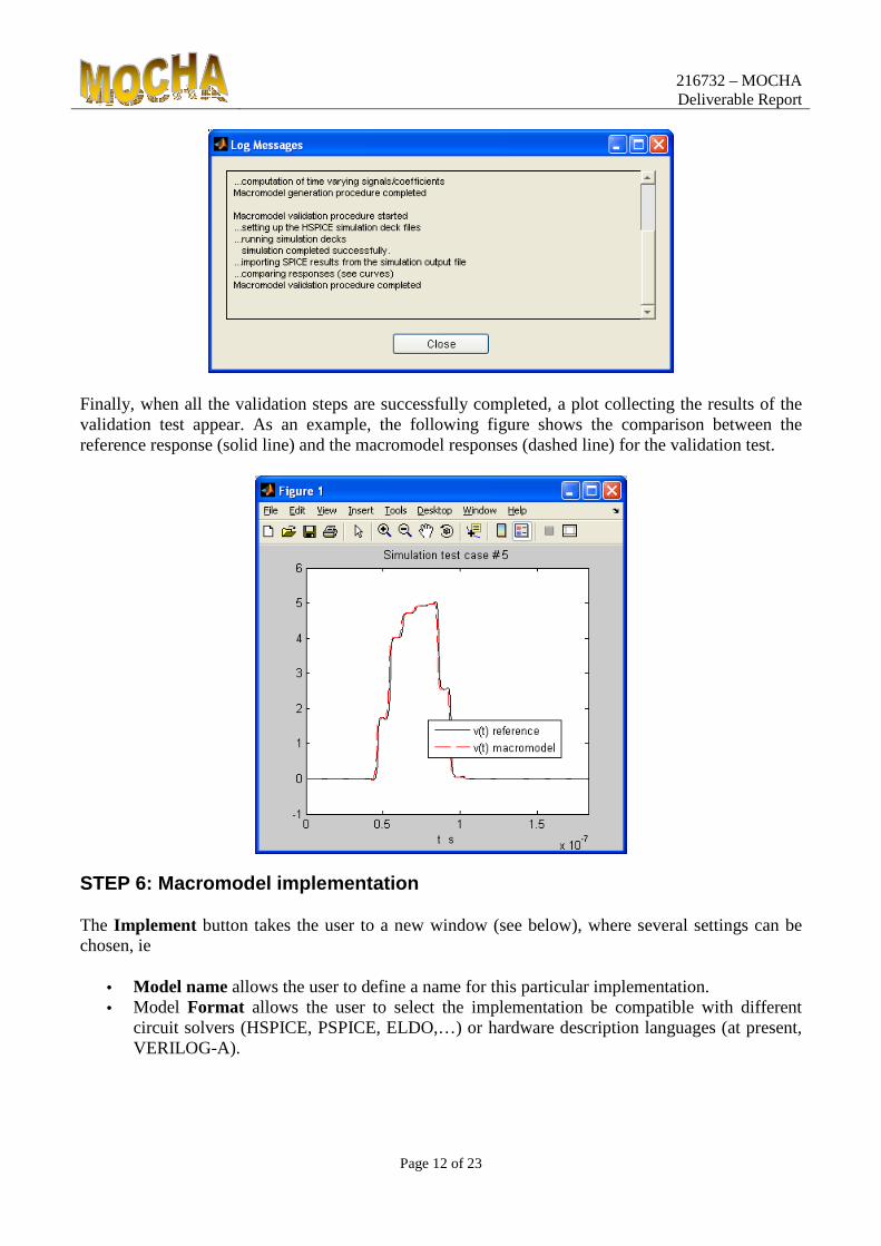
STEP 5: Macromodel validation

The Validate button allows to automatically check the accuracy of the generated model before implementing and using it. The validation is done by computing the macromodel response to simulation test cases by comparing the model response and the reference one obtained with the transitor-level description of the example device. The simulation test case consists of the example device performing two complete state transitions (bit pattern "010") while its output port is connected to a distributed transmission line and the supply pin is connected to an ideal VDD battery. More details on the test case performed are in the section labeled Test#5 in the template file "dynamic.sp".

When the Validate button is pressed, the following Log window appears where the user can follow all the steps performed during the validation phase.


of 23

Finally, when all the validation steps are successfully completed, a plot collecting the results of the validation test appear. As an example, the following figure shows the comparison between the reference response (solid line) and the macromodel responses (dashed line) for the validation test.

STEP 6: Macromodel implementation

The Implement button takes the user to a new window (see below), where several settings can be chosen, ie

• Model name allows the user to define a name for this particular implementation. • Model Format allows the user to select the implementation be compatible with different

circuit solvers (HSPICE, PSPICE, ELDO,…) or hardware description languages (at present, VERILOG-A).


of 23

The Go button generates the macromodel implementation as a new file (named by the device name specified in the Implement window). The file is created in folder "c:\temp\example1\macromodel\HSPICE" (or in subfolder VERILOG-A,... for different implementations). It is suggested that the user moves this file in the workspace of his/her preferred simulator, and starts using it.

5. Tool for the generation of models from real measured data In this Section, the set of routines used to build the models of the example test cases considered in the MOCHA project is detailed below. A pseudo-code combining textual comments and Matlab programming and figures is used. As outlined in D2.3, the modeling procedure can be divided into the following steps: (i) estimation of the buffer static characteristic isH,L; (ii) estimation of the dynamic submodels idH,L; (iii) computation of the weighting coefficients wH,L and (iv) model implementation.

Preliminary operations: clear the workspace, close all the possible open figures and assign the value of the supply voltage. close all; clear all; VDD = 1.8; %V

Load data and estimation of the buffer static characteristics isH,L. Load the device port transient current and voltage waveform obtained as suggested by the modeling procedure as in D2.3 (see Fig.5 of D2.3) and store the curves in the variables v1 and i1 . The time axis is store in the vector time . The device responses and the time axis are ressampled by using the sampling period stored in the variable T. In this example T=100e-12 (T has been decided by the sampling capabilities of the scope used for the acquisition).

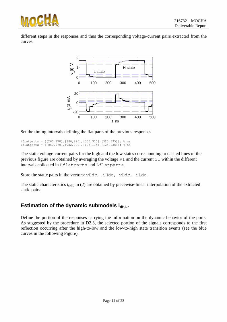
The required responses are obtained by driving the device to produces a periodic “010” bit pattern on a distributed load like a transmission line load The line length is suitably designed to allow for the response of the buffer to produce a number of steps (3-5). In such a way, the static values of the buffer characteristics are extracted from the flat parts of the response. The following Figure shows the buffer response to a distributed load consisting of the shunt connection of two identical coaxial cables (Z0=50Ω, length L=2.3m). The blue lines superimposed to the responses highlight the


of 23

different steps in the responses and thus the corresponding voltage-current pairs extracted from the curves.

0 100 200 300 400 500

0

1

2

v 1(t)

VL state

H state

0 100 200 300 400 500-20

0

20

t ns

i 1(t)

mA

Set the timing intervals defining the flat parts of the previous responses Hflatparts = [260,270],[280,290],[305,315],[325,33 5]; % ns Lflatparts = [062,070],[082,090],[105,115],[125,13 5]; % ns

The static voltage-current pairs for the high and the low states corresponding to dashed lines of the previous figure are obtained by averaging the voltage v1 and the current i1 within the different intervals collected in Hflatparts and Lflatparts .

Store the static pairs in the vectors: vHdc, iHdc, vLdc, iLdc .

The static characteristics isH,L in (2) are obtained by piecewise-linear interpolation of the extracted static pairs.

Estimation of the dynamic submodels idH,L. Define the portion of the responses carrying the information on the dynamic behavior of the ports. As suggested by the procedure in D2.3, the selected portion of the signals corresponds to the first reflection occurring after the high-to-low and the low-to-high state transition events (see the blue curves in the following Figure).


of 23

0 100 200 300 400

0

1

2

v 1(t)

V

Identification (L and H submodels)

0 100 200 300 400-20

0

20

i 1(t)

mA

t ns Define the timing intervals LIMITH = [270,275]; % ns LIMITL = [070,075]; % ns

Store the portion of the v1 and i1 signals belonging to these intervals: indH = find( time>=LIMITH(1) & time<=LIMITH(2) ) ; indL = find( time>=LIMITL(1) & time<=LIMITL(2) ) ; v2H = v2(indH); i1H = i1(indH); v1L = v1(indL); v2L = v2(indL); i1L = i1(indL);

Extract the static response and call the routines for the estimation of the models parameters defining the dynamic responses, i.e. the dynamic submodels idH,L of (2). i1Hstat = interp1(vHdc,iHdc,v1H,'linear','extrap '); % i1sH i1Lstat = interp1(vLdc,iLdc,v1L,'linear','extrap '); % i1sL OFFSETH = 1.8; NETH = estimNet_LLSS ((i1H-i1Hstat),(v1H-OFFSE TH),2,0,'NaN',T); NETL = estimNet_LLSS ((i1L-i1Lstat),v1L,2,0,'N aN',T); i1Hmod = simNet_LLSS(NETH,(v1H-OFFSETH),0); % co rresponds to i1dH i1Lmod = simNet_LLSS(NETL,v1L,0); % corresponds to i1dL

Load data and computation of the weighting coefficients wH,L

The weighting signals wH and wL are computed after the estimation of the submodels iH and iL from port responses occurring during state switchings, as discussed in [3]. In our problem, this amounts to solving the single linear equation (1) where v1 and i1 are the voltage and current responses recorded during single transition events while the device operates in regular conditions and wL is assumed to be wL = (1 - wH). In principle, such an assumption can be removed and two set of port responses can be used to compute two independent wH and wL signals. However, the latter simplification benefits the quality of the complete model since it reduces possible ill-conditioning or inaccuracies of the solution of the linear problem arising from noisy measured data or from the approximated responses of submodels iH and iL.


of 23

As an example, the following Figure shows the measured curves that can be effectively used to estimate the weighting signals and that are obtained by recording the device responses with a 50Ω termination.

0 100 200 300 400

0

1

2

v 1(t)

V

Identification (weighting signals)

0 100 200 300 400

0

10

20

i 1(t)

mA

t ns

Store in the variables v1 and i1 the responses collecting the two high-to-low and low-to-high state switching events that will be used for the estimation of the weighting coefficents. Define the intervals corresponding to the switching events and compute the weighting signals by linear inversion of (1). LIMITUP = [246.5,270]*1e-9; LIMITDN = [46.5,70]*1e-9; indUP = find( time>=LIMITUP(1) & time<=LIMITUP(2 ) ); indDN = find( time>=LIMITDN(1) & time<=LIMITDN(2 ) ); timeUP = time(indUP); timeDN = time(indDN); v1UP = v1(indUP); v1DN = v1(indDN); i1UP = i1(indUP); i1DN = i1(indDN); i1Hstat = interp1(vHdc,iHdc,v1,'linear','extrap'); i1Lstat = interp1(vLdc,iLdc,v1,'linear','extrap'); i1Hmod = simNet_LLSS(NETH,(v1-OFFSETH),0); i1Lmod = simNet_LLSS(NETL,v1,0); wH = (i1-i1Lstat-i1Lmod)./(i1Hstat+i1Hmod-i1Ls tat-i1Lmod+eps); wL = 1-wH;

Separate the weighting coefficients fro the single up and down switching events wHUP = wH(indUP); wHDN = wH(indDN); wLUP = wL(indUP); wLDN = wL(indDN); NN = min(length(wHUP),length(wHDN)); wHUP = wHUP(1:NN); wHDN = wHDN(1:NN); wLUP = wLUP(1:NN); wLDN = wLDN(1:NN);

If needed, the weighting signals wHUP, wHDN, wLUP, wLDN can be effectively approximated by means of simple analytical functions. It is worth noting that, to possibly reduce the effects of


of 23

measurement errors, the analytical approximation of the weighting signal by means of smooth functions contribute to the improvement of the model accuracy. Also, due to the typical smooth sigmoidal shape of the weighting signals, the approximation carried out by means of a tanh function and two gaussian functions has been proven to be enough to provide accurate results. Assign the variables collecting model parameters MOD.T = T; MOD.NET_H = NETH; MOD.NET_L = NETL; MOD.dcH.v = [-VDD/2,0, vHdc,VDD+VDD/2]; MOD.dcH.i = interp1(vHdc,iHdc,MOD.dcH.v,'linear' ,'extrap'); MOD.dcL.v = [-VDD/2,vLdc,VDD, VDD+VDD/2]; MOD.dcL.i = interp1(vLdc,iLdc,MOD.dcL.v,'linear' ,'extrap'); MOD.wH = wH; MOD.wL = wL; MOD.wHu = wHUP; MOD.wHd = wHDN; MOD.wLu = wLUP; MOD.wLd = wLDN; MOD.VDD = 1.8; MOD.BASENAME = 'drvmodmeas'; MOD.tin = 1e-9;

Model implementation Call the function that generates the HSPICE implementation of the model: sedrv_MOD2HSPICE_measurements(MOD,'./);

It is worth noting that the models obtained by means of this detailed procedure has been used to produce the responses collected in the deliverable D2.3 (Report collecting the guidelines for the generation of a test board for the generation of IC port models from measurements. Two test-cases models extracted by measurement).

Auxiliary functions: %%%%%%%%%%%%%%%%%%%%%%%%%%%%%%%%%%%%%%%%%%%%%%%%%%%%%%%%%%%%%%%%%%%%%%%%%%%%%%%%%%%%%%%%%%%%%%%%%%%%% function NSS = estimNet_LLSS (y0,U0,NN,FLAGFIG,Ts) % for the model generation from measured data, a si mple linear model is chosen for the dynamic part. % It corresponds to p=1 (see the details on the mod el structure in D2.1). %%%%%%%%%%%%%%%%%%%%%%%%%%%%%%%%%%%%%%%%%%%%%%%%%%%%%%%%%%%%%%%%%%%%%%%%%%%%%%%%%%%%%%%%%%%%%%%%%%%%% % NN = 'best' or fix value (e.g., NN=1) % INITIAL LINEAR ESTIMATION BY USING 4SID METHOD (V heragen,1994) Ninit = size(y0,1); DATA = iddata(y0(1:Ninit,:),U0(1:Ninit,:),Ts); m = size(U0,2); no = size(y0,2); MODEL = n4sid(DATA,NN,... 'nk',zeros(1,m),'DisturbanceModel','None',' N4Weight',... 'MOESP','CovarianceMatrix','None','InitialS tate','Estimate'); % max order allowed: 3 n=size(MODEL.A,1); if n>3


of 23

n=3; MODEL = n4sid(DATA,n,... 'nk',zeros(1,m),'DisturbanceModel','Non e','N4Weight',... 'MOESP','CovarianceMatrix','None','Init ialState','Estimate'); end % NSS MODEL INITIALIZATION... NSS.n = size(MODEL.A,1); NSS.no = no; NSS.m = m; NSS.A = MODEL.A; NSS.B = MODEL.B; NSS.C = MODEL.C; NSS.D = MODEL.D; % FORCE DC STAT CHAR = 0... NSS.D = -NSS.C*inv(eye(size(NSS.A))-NSS.A)*NSS.B; ymod = simNet_4SID(NSS,U0,y0(1)); if FLAGFIG==1 graphNet(y0,ymod,NSS.n); end %================================================== ==================================== function graphNet(y,ymod,n) %================================================== ==================================== no = size(y,2); str=['order ',num2str(n)]; hfig = figure; set(hfig,'UserData','myplot'); for kk=1:no subplot(no,1,kk) plot(y(:,kk),'k-') hold on plot(ymod(:,kk),'r--') hold off; set(gca,'xlim',[1,length(y)]); if kk==no xlabel('samples'); end ylabel(['normalized response i_',num2str(kk)]) if kk==1 title(str); legend('reference','model'); end end

%%%%%%%%%%%%%%%%%%%%%%%%%%%%%%%%%%%%%%%%%%%%%%%%%%%%%%%%%%%%%%%%%%%%%%%%%%%%%%%%%%%%%%%%%%%%%%%%%%%%% function ymod = simNet_LLSS(NSS,U,y0) % for the model generation from measured data, a si mple linear model is chosen for the dynamic part. % It corresponds to p=1 (see the details on the mod el structure in D2.1). %%%%%%%%%%%%%%%%%%%%%%%%%%%%%%%%%%%%%%%%%%%%%%%%%%%%%%%%%%%%%%%%%%%%%%%%%%%%%%%%%%%%%%%%%%%%%%%%%%%%% n = NSS.n; no = NSS.no; m = NSS.m; N = length(U); % evaluate x0 i.c. x0 = inv(eye(n)-NSS.A)*(NSS.B*U(1,:)'); % response X = [x0';zeros(N-1,n)]; ymod = zeros(N,no); xprev = X(1,:)'; uprev = U(1,:)'; %tic; for kk = 2:N ukk = U(kk,:)';


of 23

xkk = NSS.A*xprev + NSS.B*uprev ; ymod(kk,:) = NSS.C*xkk + NSS.D*ukk; X(kk,:) = xkk'; xprev = xkk; uprev = ukk; end %tsim = toc; % disp([' simulation time = ',num2str(tsim),' sec.' ]); ymod(1,:) = ymod(2,:);

%%%%%%%%%%%%%%%%%%%%%%%%%%%%%%%%%%%%%%%%%%%%%%%%%%%%%%%%%%%%%%%%%%%%%%%%%%%%%%%%%%%%%%%%%%%%%%%%%%%%% function sedrv_MOD2HSPICE_measurements(MOD,MYPATH); %%%%%%%%%%%%%%%%%%%%%%%%%%%%%%%%%%%%%%%%%%%%%%%%%%%%%%%%%%%%%%%%%%%%%%%%%%%%%%%%%%%%%%%%%%%%%%%%%%%%% format long e form = '%2.14e'; T = MOD.T; VDD = MOD.VDD; filename=[MOD.BASENAME,'.lib']; tw=T*[0:length(MOD.wHu)-1]'; TMIN=tw(end); wHu=MOD.wHu; wHd=MOD.wHd; wLu=MOD.wLu; wLd=MOD.wLd; TIPODIMODELLO='Output-port driver macromodel '; STRUCTURE='nonlinear static + dynamic)'; FID = fopen(fullfile(MYPATH,filename),'wt'); str=['* ',TIPODIMODELLO,' (',STRUCTURE,'), ',date]; fprintf(FID,'%s\n',str); str=['* HSPICE implementation autogenerated by Mpil og (MODEL FORM MEASUREMENTS)']; fprintf(FID,'%s\n',str); str=['***************************************** *********** ']; fprintf(FID,'\n%s\n',str); str=['* COMPLETE MACROMODEL ']; fprintf(FID,'%s\n',str); str=['***************************************** *********** ']; fprintf(FID,'%s\n',str); str=['.subckt ',MOD.BASENAME,' in v vdd ref']; fprintf(FID,'%s\n\n',str); str=['.PARAM Ts = ',num2str(T,form)]; fprintf(F ID,'%s\n',str); str=['.PARAM Rx = 1']; fprintf(FID,'%s\n',str); str=['.PARAM step(x) = ''(1/2)*(1+sgn(x))''' ]; fprintf(FID,'%s\n',str); str=['.PARAM port(x,y,z) = ''step(x+(-1)*y) - step(x+(-1)*z)''']; fprintf(FID,'%s\n\n',str); %str=['**************************************** ************ ']; fprintf(FID,'\n%s\n',str); %str=['* "bit" cuncatenation... ']; fprintf(FID ,'\n%s\n',str); %str=['**************************************** ************ ']; fprintf(FID,'\n%s\n',str); %str=['* create V(in1) = normazlized V(in)']; f printf(FID,'%s\n',str); str=[' Ein2 in2 0 vol=''V(in,0)/',num2str(MOD. VDD),'-0.5''']; fprintf(FID,'%s\n',str); str=[' Ein1 in1 0 vol=''0.5*(1+sgn(V(in2)))''' ]; fprintf(FID,'%s\n',str); %str=['* normalize the digital input signal in the range [-1,1]']; fprintf(FID,'%s\n',str); str=[' GIN 0 2 cur=''2*(V(in1)-0.5)''']; fprin tf(FID,'%s\n',str); %str=['* design an ideal integrator']; fprintf( FID,'%s\n',str); str=[' RIN 2 0 1e6']; fprintf(FID,'%s\n',str); str=[' CIN 2 0 ',num2str(TMIN),' ic=0']; fprin tf(FID,'%s\n',str); %str=['* V(1,0) can be used to sweep the time o f the up and down sequences']; fprintf(FID,'%s\n',str); str=[' XD1 21 2 IDDIODE_',MOD.BASENAME]; fprin tf(FID,'%s\n',str); str=[' VD1 21 0 0']; fprintf(FID,'%s\n',str); str=[' XD2 2 22 IDDIODE_',MOD.BASENAME]; fprin tf(FID,'%s\n',str); str=[' VD2 22 0 1']; fprintf(FID,'%s\n',str); %str=['* create 1-V(1,0)']; fprintf(FID,'%s\n', str); str=[' E1 1 0 vol='' V(2,0) + (',num2str(M OD.tin/2/TMIN,form),') ''']; fprintf(FID,'%s\n',str); str=[' E111 111 0 vol='' 1 - V(2,0) + (',num2s tr(MOD.tin/2/TMIN,form),') ''']; fprintf(FID,'%s\n\n',str);


of 23

str=[' Ew1 w1 0 vol=''V(in1)*V(wu1)+(1-V(in1)) *V(wd1)''']; fprintf(FID,'%s\n',str); str=[' Ew2 w2 0 vol=''V(in1)*V(wu2)+(1-V(in1)) *V(wd2)''']; fprintf(FID,'%s\n',str); str=['*** model structure...']; fprintf(FID,'\n %s\n',str); str=['Gy1 vdd y1 cur='' V(w1)*( V(f1) + V(fs1) ) ''']; fprintf(FID,'%s\n',str); str=['Gy2 ref y2 cur='' V(w2)*( V(f2) + V(fs2) ) ''']; fprintf(FID,'%s\n',str); str=['Rc1 ref v 1e6']; fprintf(FID,'%s\n',str); str=['Rc2 ref vdd 1e6']; fprintf(FID,'%s\n',str ); str=['Ry1 y1 y Rx']; fprintf(FID,'%s\n',str); str=['Ry2 y2 y Rx']; fprintf(FID,'%s\n',str); str=['Ry y v Rx']; fprintf(FID,'%s\n',str); % INPUT VARIABLES... str=['*** input variables...']; fprintf(FID,'\n %s\n',str); str=['Ru1 u1 0 Rx']; fprintf(FID,'%s\n',str); str=['Eu1 u1 0 vol=''V(v,vdd)''']; fprintf(FID,'%s\n\n',str); str=['Ru2 u2 0 Rx']; fprintf(FID,'%s\n',str); str=['Eu2 u2 0 vol=''V(v,ref)''']; fprintf(FID,'%s\n\n',str); str=['*** 4SID submodels']; fprintf(FID,'\n\n%s \n\n',str); str=['* fH (f1), order = ',num2str(MOD.NET_H.n) ]; fprintf(FID,'%s\n',str); str=['XfH f1 u1 ',MOD.BASENAME,'_fH']; fprintf( FID,'%s\n',str); str=['* fL (f2), order = ',num2str(MOD.NET_L.n) ]; fprintf(FID,'%s\n',str); str=['XfL f2 u2 ',MOD.BASENAME,'_fL']; fprintf( FID,'%s\n',str); str=['*** Static characteristics: PULL-UP & PUL L-DOWN...']; fprintf(FID,'\n%s\n',str); tol = 1e-4; dv = 5e-3; str=['Rfs1 fs1 0 1'];fprintf(FID,'%s\n',str); str=['Efs1 fs1 0 PWL(1) v vdd'];fprintf(FID,'%s \n',str); for k=1:length(MOD.dcH.v) str=['+ ',num2str(MOD.dcH.v(k)-VDD,'%2.14e'),', ',num2str(MOD.dcH.i(k),'%2.14e')]; fprintf(FID,'%s\n',str); end; str=['Rfs2 fs2 0 1'];fprintf(FID,'%s\n',str); str=['Efs2 fs2 0 PWL(1) v ref'];fprintf(FID,'%s \n',str); for k=1:length(MOD.dcL.v) str=['+ ',num2str(MOD.dcL.v(k),'%2.14e'),', ',n um2str(MOD.dcL.i(k),'%2.14e')]; fprintf(FID,'%s\n',str); end; str=['*** Weighting functions...']; fprintf(FID ,'\n%s\n',str); str=['Eyu yu 0 vol=''V(1,0) ''']; fprintf(FID,' \n%s\n',str); str=['Eyd yd 0 vol=''V(111,0) ''']; fprintf(FID ,'%s\n\n',str); str=['*** Weighting functions...']; fprintf(FID ,'\n%s\n',str); statcharport2HSPICE('wu','1',FID,tw/TMIN,wHu,fo rm,['yu 0'],' V(yu) '); statcharport2HSPICE('wd','1',FID,tw/TMIN,wHd,fo rm,['yd 0'],' V(yd) '); statcharport2HSPICE('wu','2',FID,tw/TMIN,wLu,fo rm,['yu 0'],' V(yu) '); statcharport2HSPICE('wd','2',FID,tw/TMIN,wLd,fo rm,['yd 0'],' V(yd) '); str=['.ends']; fprintf(FID,'%s\n\n',str); %------------------------------------------ str=['***************************************** *********** ']; fprintf(FID,'%s\n',str); str=['* LLSS SUBCIRCUITS (p=1) ']; fprintf(FID,'%s\n',str); str=['***************************************** *********** ']; fprintf(FID,'%s\n\n',str); submodelMIMO_LLSS2HSPICE([MOD.BASENAME,'_fH'],T ,MOD.NET_H,FID,form); submodelMIMO_LLSS2HSPICE([MOD.BASENAME,'_fL'],T ,MOD.NET_L,FID,form); %------------------------------------------ str=['***************************************** *********** ']; fprintf(FID,'%s\n',str); str=['* AUX SUBMODELS ']; fprintf(FID,'%s\n',str); str=['***************************************** *********** ']; fprintf(FID,'%s\n',str);


of 23

str=['.subckt IDDIODE_',MOD.BASENAME,' 1 2']; f printf(FID,'%s\n',str); str=['.PARAM step(x) = ''(1/2)*(1+sgn(x))''' ];fprintf(FID,'%s\n',str); str=['.PARAM a = 1e6'];fprintf(FID,'%s\n',str); str=[' Gd 1 2 cur=''a*POW(V(1,2),2)*step(V(1,2) )'''];fprintf(FID,'%s\n',str); str=['.ends'];fprintf(FID,'%s\n\n',str); str=['*.subckt IDDIODE_',MOD.BASENAME,' 1 2']; fprintf(FID,'%s\n',str); str=['*Gd 1 2 PWL(1) 1 2'];fprintf(FID,'%s\n',s tr); str=['*+ -1, 0'];fprintf(FID,'%s\n',str); str=['*+ 0, 0'];fprintf(FID,'%s\n',str); str=['*+ 1e-6, 1e6'];fprintf(FID,'%s\n',str); str=['*.ends'];fprintf(FID,'%s\n\n',str); ST=fclose(FID); format; %%%%%%%%%%%%%%%%%%%%%%%%%%%%%%%%%%%%%%%%%%%%%%%%%%%%%%%%%%%%%%%%%%%%%%%%%%%%%%%%%%%%%%%%%%%%%%%%%%%%%function submodelMIMO_LLSS2HSPICE(BASENAME,T,NET,FID,form); % function for p=1 only %%%%%%%%%%%%%%%%%%%%%%%%%%%%%%%%%%%%%%%%%%%%%%%%%%%%%%%%%%%%%%%%%%%%%%%%%%%%%%%%%%%%%%%%%%%%%%%%%%%%% str=['.subckt ',BASENAME]; for nn=1:NET.no str=[str,' f',num2str(nn)]; end for mm=1:NET.m str=[str,' u',num2str(mm)]; end fprintf(FID,'%s\n',str); str=['.PARAM Ts = ',num2str(T,form)]; fprintf(F ID,'%s\n',str); str=['.PARAM Rx = 1']; fprintf(FID,'%s\n\n',str ); % STATE VARIABLES... str=['* state variables...']; fprintf(FID,'%s\n ',str); str=['* x','1,...,x',num2str(NET.n)]; fprintf(F ID,'%s\n\n',str); for kn=1:NET.n str=['* x',num2str(kn)]; fprintf(FID,'%s\n',str ); str=[' Rx',num2str(kn),' x',num2str(kn),' 0 Rx ']; fprintf(FID,'%s\n',str); str=[' Cx',num2str(kn),' x',num2str(kn),' 0 Ts ']; fprintf(FID,'%s\n',str); str=[' Gx',num2str(kn),' 0 x',num2str(kn),' cu r=''V(fx',num2str(kn),')/Rx''']; fprintf(FID,'%s\n\n',str); end; str=['*** State-Space models...']; fprintf(FID, '%s\n\n',str); str=['*(1) state equation...']; fprintf(FID,'%s \n\n',str); for ii=1:NET.n str=[' Rfx',num2str(ii),' 0 fx',num2str(ii ),' Rx']; fprintf(FID,'%s\n',str); str=[' Gfx',num2str(ii),' 0 fx',num2str(ii ),' cur=''0\\']; fprintf(FID,'%s\n',str); for jj=1:NET.n str=[' +(',num2str(NET.A(ii,jj),form),')*V (x',num2str(jj),')\\']; fprintf(FID,'%s\n',str); end; for jj=1:NET.m str=[' +(',num2str(NET.B(ii,jj),form),')*V (u',num2str(jj),')\\']; fprintf(FID,'%s\n',str); end; str=[' ''']; fprintf(FID,'%s\n\n',str); end; str=['*(2) output equation...']; fprintf(FID,'% s\n\n',str); for nn=1:NET.no str=[' Rf',num2str(nn),' 0 f',num2str(nn),' Rx ']; fprintf(FID,'%s\n',str); str=[' Gf',num2str(nn),' 0 f',num2str(nn),' cu r=''0\\']; fprintf(FID,'%s\n',str); for jj=1:NET.n str=[' +(',num2str(NET.C(nn,jj),form),')*V(x', num2str(jj),')\\']; fprintf(FID,'%s\n',str); end; if (~isempty(NET.D))&(NET.D~=0) for jj=1:NET.m str=[' +(',num2str(NET.D(nn,jj),form),')*V(u', num2str(jj),')\\']; fprintf(FID,'%s\n',str);


of 23

end; end; str=[' ''']; fprintf(FID,'%s\n\n',str); end; str=['.ends']; fprintf(FID,'%s\n\n',str); %%%%%%%%%%%%%%%%%%%%%%%%%%%%%%%%%%%%%%%%%%%%%%%%%%%%%%%%%%%%%%%%%%%%%%%%%%%%%%%%%%%%%%%%%%%%%%%%%%%%% function statcharport2HSPICE(NAME,LABEL,FID,dcV,dcI,form,INPUT1,INPUT2); %%%%%%%%%%%%%%%%%%%%%%%%%%%%%%%%%%%%%%%%%%%%%%%%%%%%%%%%%%%%%%%%%%%%%%%%%%%%%%%%%%%%%%%%%%%%%%%%%%%%% % # points of static characteristic data... LV = length(dcV); a1 = (dcI(2)-dcI(1))/(dcV(2)-dcV(1)); b1 = dcI(1) - a1*dcV(1); a2 = (dcI(end)-dcI(end-1))/(dcV(end)-dcV(end-1)); b2 = dcI(end) - a2*dcV(end); if (LV<=100) % # points less than 100 str=['R',NAME,LABEL,' ',NAME,LABEL,' 0 1']; fpri ntf(FID,'%s\n',str); kk=1; str=['G',NAME,LABEL,num2str(kk),' 0 ',NAME,LABEL ,' cur = ''\\']; fprintf(FID,'%s\n',str); str=['V(',NAME,LABEL,num2str(kk),')*( port(',INPUT2,',(',num2str(dcV(1),form),'),(',num2s tr(dcV(end),form),')) )''']; fprintf(FID,'%s\n\n',str); str=['Gstep',NAME,LABEL,num2str(1),' 0 ',NAME,LA BEL,' cur = ''\\']; fprintf(FID,'%s\n',str); str=['( (',num2str(a1,form),')*',INPUT2,' + (',n um2str(b1,form),') )*step( -1*',INPUT2,' + (',num2str(dcV(1),form),') )']; fprintf(FID,'%s\n\n',str); str=['Gstep',NAME,LABEL,num2str(2),' 0 ',NAME,LA BEL,' cur = ''\\']; fprintf(FID,'%s\n',str); str=['( (',num2str(a2,form),')*',INPUT2,' + (',n um2str(b2,form),') )*step( ',INPUT2,' - (',num2str(dcV(end),form),') )']; fprintf(FID,'%s\n\n',str); str=['Rx',NAME,LABEL,'1 ',NAME,LABEL,'1 0 1']; f printf(FID,'%s\n',str); str=['Gx',NAME,LABEL,'1 0 ',NAME,LABEL,'1 PWL(1) ',INPUT1]; fprintf(FID,'%s\n',str); for jj=1:LV str=['+ ',num2str(dcV(jj),form),', ',num2str (dcI(jj),form)]; fprintf(FID,'%s\n',str); end else % # points more than 100 Nbreaks = floor(LV/99); vbreaks = 100 + 99*[0:1:Nbreaks-1]'; str=['R',NAME,LABEL,' ',NAME,LABEL,' 0 1']; fpri ntf(FID,'%s\n',str); kk = 1; str=['G',NAME,LABEL,num2str(kk),' 0 ',NAME,LABEL ,' cur = ''\\']; fprintf(FID,'%s\n',str); str=['V(',NAME,LABEL,num2str(kk),')*( port(',INPUT2,',(',num2str(dcV(1),form),'),(',num2s tr(dcV(vbreaks(kk)),form),')) )''']; fprintf(FID,'%s\n\n',str); for kk=2:Nbreaks str=['G',NAME,LABEL,num2str(kk),' 0 ',NAME,L ABEL,' cur = ''\\']; fprintf(FID,'%s\n',str); str=['V(',NAME,LABEL,num2str(kk),')*( port(' ,INPUT2,',(',num2str(dcV(vbreaks(kk-1)),form),'),(',num2str(dcV(vbreaks(kk)),form),')) )''']; fprintf(FID,'%s\n\n',str); end kk = Nbreaks+1; str=['G',NAME,LABEL,num2str(kk),' 0 ',NAME,LABEL ,' cur = ''\\']; fprintf(FID,'%s\n',str); str=['V(',NAME,LABEL,num2str(kk),')*( port(',INP UT2,',(',num2str(dcV(vbreaks(kk-1)),form),'),(',num2str(dcV(end),form),')) )''']; fprintf(FID,'%s\n\n',str); str=['Gstep',NAME,LABEL,num2str(1),' 0 ',NAME,LA BEL,' cur = ''\\']; fprintf(FID,'%s\n',str); str=['( (',num2str(a1,form),')*',INPUT2,' + (',n um2str(b1,form),') )*step( -1*',INPUT2,' + (',num2str(dcV(1),form),') )''']; fprintf(FID,'%s\n\n',str); str=['Gstep',NAME,LABEL,num2str(2),' 0 ',NAME,LA BEL,' cur = ''\\']; fprintf(FID,'%s\n',str); str=['( (',num2str(a2,form),')*',INPUT2,' + (',n um2str(b2,form),') )*step( ',INPUT2,' - (',num2str(dcV(end),form),') )''']; fprintf(FID,'%s\n\n',str);


of 23

str=['Rx',NAME,LABEL,'1 ',NAME,LABEL,'1 0 1']; f printf(FID,'%s\n',str); str=['Gx',NAME,LABEL,'1 0 ',NAME,LABEL,'1 PWL(1) ',INPUT1]; fprintf(FID,'%s\n',str); for jj=1:vbreaks(1) str=['+ ',num2str(dcV(jj),form),', ',num2str (dcI(jj),form)]; fprintf(FID,'%s\n',str); end for kk=2:Nbreaks str=['Rx',NAME,LABEL,num2str(kk), ' ',NAME,L ABEL,num2str(kk),' 0 1']; fprintf(FID,'%s\n',str); str=['Gx',NAME,LABEL,num2str(kk), ' 0 ',NAME ,LABEL,num2str(kk),' PWL(1) ',INPUT1]; fprintf(FID,'%s\n',str); for jj=vbreaks(kk-1):vbreaks(kk) str=['+ ',num2str(dcV(jj),form),', ',num 2str(dcI(jj),form)]; fprintf(FID,'%s\n',str); end end str=['Rx',NAME,LABEL,num2str(Nbreaks+1),' ',NAME ,LABEL,num2str(Nbreaks+1),' 0 1']; fprintf(FID,'%s\n',str); str=['Gx',NAME,LABEL,num2str(Nbreaks+1),' 0 ',NA ME,LABEL,num2str(Nbreaks+1), ' PWL(1) ',INPUT1]; fprintf(FID,'%s\n',str); for jj=vbreaks(end):LV str=['+ ',num2str(dcV(jj),form),', ',num2str (dcI(jj),form)]; fprintf(FID,'%s\n',str); end str = ['***']; fprintf(FID,'%s\n\n',str); end str = ['***']; fprintf(FID,'%s\n\n',str);

References [1] I. S. Stievano et Al. , "Behavioral modeling of digital devices via composite local-linear state-space relations," IEEE

Transactions on Instrumentation and Measurement, Vol. 57, No. 8, 2008.

[2] I. S. Stievano, I. A. Maio, F. G. Canavero, “Behavioral models of IC output buffers from on-the-fly measurements,” IEEE Transactions on Instrumentation and Measurement, vol. 57, No. 4, pp. 850-855, 2008.

[3] MOCHA Deliverable D2.1, “Report describing the structure of the new parametric model for digital ICs and detailed procedure for model validation”, Oct. 2008.

[4] MOCHA Deliverable D2.3, “Report collecting the guidelines for the generation of a test board for the generation of IC port models from measurements. Two test-cases models extracted by measurement”, Jul. 2009.

[5] Jan M. Rabaey, “Digital Integrated Circuits - 2nd ed.”, Prentice Hall electronics and VLSI series, 2003.

mocha wp2 deliverable d2 - cordiscordis.europa.eu/.../mocha-wp2-deliverable-d2-4.pdfthis section is...

Documents