modal interactions of a three-degree-of-freedom system...
TRANSCRIPT

Nonlinear DynDOI 10.1007/s11071-015-2343-3
ORIGINAL PAPER
N − 1 modal interactions of a three-degree-of-freedomsystem with cubic elastic nonlinearities
X. Liu · A. Cammarano · D. J. Wagg ·S. A. Neild · R. J. Barthorpe
Received: 11 May 2015 / Accepted: 20 August 2015© The Author(s) 2015. This article is published with open access at Springerlink.com
Abstract In this paper the N − 1 nonlinear modalinteractions that occur in a nonlinear three-degree-of-freedom lumped mass system, where N = 3, areconsidered. The nonlinearity comes from springs withweakly nonlinear cubic terms. Here, the case where allthe natural frequencies of the underlying linear systemare close (i.e. ωn1 : ωn2 : ωn3 ≈ 1 : 1 : 1) is con-sidered. However, due to the symmetries of the sys-tem under consideration, only N − 1 modes interact.Depending on the sign and magnitude of the nonlin-ear stiffness parameters, the subsequent responses canbe classified using backbone curves that represent theresonances of the underlying undamped, unforced sys-tem. These backbone curves, which we estimate ana-lytically, are then related to the forced response of thesystem around resonance in the frequency domain. Theforced responses are computed using the continuationsoftware AUTO-07p. A comparison of the results gives
X. Liu (B) · D. J. Wagg · R. J. BarthorpeDepartment of Mechanical Engineering, University ofSheffield, Sheffield S1 3JD, UKe-mail: [email protected]
D. J. Wagge-mail: [email protected]
A. CammaranoSchool of Engineering, University of Glasgow, GlasgowG12 8QQ, UK
S. A. NeildDepartment of Mechanical Engineering, University of Bristol,Bristol BS8 1TR, UK
insights into the multi-modal interactions and showshow the frequency response of the system is related tothose branches of the backbone curves that representsuch interactions.
Keywords 3-DoF nonlinear oscillator · Backbonecurve · Nonlinear modal interaction · Second-ordernormal form method
1 Introduction
Understanding the effects of modal interactions of cou-pled systems of nonlinear equations is an importantstep in being able to predict the subsequent dynamicresponse of the system. In this paper, we considera three-degree-of-freedom (3-DoF) lumped mass sys-temwith cubic stiffness nonlinearities. In particular weconsider the potential forced responses that can occurby analysing the backbone curves of the underlyingundamped, unforced system. The justification of thisapproach lies in that the vast majority of engineeringstructures is characterised by low level of damping.This implies that their dynamical behaviour is largelydetermined by the dynamics of the associated Hamil-tonian system [10].
The motivation for this study is the possibilityfor modes, in multi-degree-of-freedom nonlinear sys-tems, to interact with each other [17]. These typesof modal interaction have been previously studiedbecause they are often related to unwanted vibrationeffects in engineering structures [16]. The majority of
123
X. Liu et al.
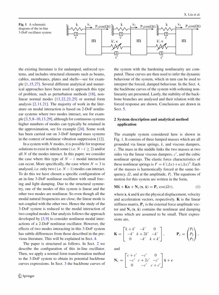
Fig. 1 A schematicdiagram of the in-line3-DoF oscillator system
the existing literature is for undamped, unforced sys-tems, and includes structural elements such as beams,cables, membranes, plates and shells—see for exam-ple [1,15,27]. Several different analytical and numer-ical approaches have been used to approach this typeof problem, such as perturbation methods [18], non-linear normal modes [13,22,23,25] or normal formanalysis [2,11,21]. The majority of work in the liter-ature on modal interaction is based on 2-DoF nonlin-ear systems where two modes interact, see for exam-ple [3,5,8–10,13,29], although for continuous systemshigher numbers of modes can typically be retained inthe approximation, see for example [24]. Some workhas been carried out on 3-DoF lumped mass systemsin the context of nonlinear vibration suppression [12].
In a systemwith N modes, it is possible for responsesolutions to exist in which some ( i.e. N−i ≥ 2) and/orall N of the modes interact. In this paper, we considerthe case where this type of N − i modal interactioncan occur. More specifically, the case where N = 3 isanalysed, i.e. only two ( i.e. N −1) modes can interact.To do this we have chosen a specific configuration ofan in-line 3-DoF nonlinear oscillator with small forc-ing and light damping. Due to the structural symme-try, one of the modes of this system is linear and theother two modes are nonlinear. So even though all themodal natural frequencies are close, the linear mode isnot coupled with the other two. Hence the study of the3-DoF system is reduced to the modal interaction oftwo coupled modes. Our analysis follows the approachdeveloped by [3,9] to consider nonlinear modal inter-actions of a 2-DoF nonlinear oscillator. However, theeffects of two modes interacting in this 3-DoF systemhas subtle differences from those described in the pre-vious literature. This will be explained in Sect. 4.
The paper is structured as follows. In Sect. 2 wedescribe the configuration of this in-line oscillator.Then, we apply a normal form transformation methodto the 3-DoF system to obtain its potential backbonecurves expressions. In Sect. 3 the backbone curves of
the system with the hardening nonlinearity are com-puted. These curves are then used to infer the dynamicbehaviour of the system, which in turn can be used tointerpret the forced, damped behaviour. In the Sect. 4,the backbone curves of the system with softening non-linearity are presented. Lastly, the stability of the back-bone branches are analysed and their relation with theforced response are shown. Conclusions are drawn inSect. 5.
2 System description and analytical methodapplication
The example system considered here is shown inFig. 1. It consists of three lumped masses which are allgrounded via linear springs, k, and viscous dampers,c. The mass in the middle links the two masses at twosides via the linear viscous dampers, c′, and the cubicnonlinear springs. The elastic force characteristics ofthese nonlinear springs is F = k′(Δx)+κ(Δx)3. Eachof the masses is harmonically forced at the same fre-quency, Ω , and at the amplitude, Pi . The equations ofmotion for this system are written in the form,
Mx + Kx + Nx (x, x) = Px cos(Ωt), (1)
where x, x and x are the physical displacement, velocityand acceleration vectors, respectively. K is the linearstiffness matrix, Px is the external force amplitude vec-tor and Nx (x, x) contains the nonlinear and dampingterms which are assumed to be small. Their expres-sions are,
K =⎡⎣k + k′ −k′ 0−k′ k + 2k′ −k′0 −k′ k + k′
⎤⎦ , Px =
⎛⎝P1P2P3
⎞⎠ ,
and
Nx =⎡⎣c + c′ −c′ 0−c′ c + 2c′ −c′0 −c′ c + c′
⎤⎦ x + κ
123

N − 1 modal interactions of a three-degree-of-freedom system
⎛⎝
(x1 − x2)3
(x2 − x1)3 + (x2 − x3)3
(x3 − x2)3
⎞⎠ .
To proceed, the second-order normal form method isapplied to approximately solve the equations of motionof this system. First, in order to decouple the linearterms, the linear modal transformation is applied toEq. 1 to obtain the linear modal decomposition equa-tions in terms of the new modal state q = {q1 q2 q3}Tas,
q + Λq + Nq(q, q) = Pq cos(Ωt), (2)
where Λ is a diagonal matrix of the squares of thecorresponding linear natural frequencies ω2
n1 = k/m,ω2n2 = (k + k′)/m and ω2
n3 = (k + 3k′)/m. Nq is thevector containing the damping and nonlinear couplingterms,
Nq =⎛⎝2ωn1ζ1q12ωn2ζ2q22ωn3ζ3q3
⎞⎠+ μ
⎛⎝
0q32 + 27q2q239q22q3 + 27q33
⎞⎠ , (3)
whereμ = κ/m, 2ωn1ζ1 = c/m, 2ωn2ζ2 = (c+c′)/mand 2ωn3ζ3 = (c + 3c′)/m. In the modal coor-dinates, the external force amplitude vector, Pq ={Pm1 Pm2 Pm3}T , is
Pq = Φ−1M−1Px = 1
6m
⎡⎣2 2 23 0 −31 −2 1
⎤⎦Px , (4)
where Φ is the matrix of the linear modeshapes. Herethe modeshapes used for the linear transformation are{1, 1, 1}T , {1, 0, −1}T and {1, −2, 1}T for the threemodes, respectively.
Then, the forcing transformation, q → v, is sup-posed to be applied to remove the non-resonant forcingterms. Here we assume that the system is forced nearresonance, this allows us to set q = v. Substituting thisinto Eq. 2 gives,
v + Λv + Nv(v, v) = Pv cos(Ωt), (5)
where Nv(v, v) = Nq(q, q) and Pv = Pq .Lastly, applying the near-identity nonlinear trans-
form v → u to Eq. 5 by using v = u + H(u, u) givesthe equation,
u + Λu + Nu(u, u) = Pu cos(Ωt), (6)
where Pu = Pq and Nu = nuu∗ includes only thenonlinear resonant terms responding at the fundamen-tal frequency of the corresponding modes. Here u and
H(u, u) used in the transformation are the fundamentaland harmonic components of v, respectively. Substitut-ing vi → ui = uip +uim into Eq. 3 in v gives the func-tional form of the u∗ vector and the coefficient matrixnv so that Nv = nvu∗ as below, where the subscript irepresents the i th linear mode.
Then the homological equation is used to computea matrix, β, for determining the resonance terms in thenear-identity transformation [21]. The individual βi,l
terms, can be computed using,
βi,l =[
N∑n=1
{(snpl − snml)ωrn
}]2 − ω2ri , (7)
where the subscript l denotes the l th term of u∗, writ-ten as u∗
l and snpl and snml represent the power indicesof unp and unm of the term u∗
l , respectively. Finally thevariable, r , that describes the ratio between the responsefrequencies of mode 2 and 3, i.e. r = ωr3/ωr2, is intro-duced, so that for the example considered here β is,
u∗v =
⎡⎢⎢⎢⎢⎢⎢⎢⎢⎢⎢⎢⎢⎢⎢⎢⎢⎢⎢⎢⎢⎢⎢⎢⎢⎢⎢⎢⎢⎢⎢⎢⎢⎢⎢⎢⎢⎢⎢⎢⎢⎢⎢⎢⎢⎢⎢⎢⎢⎢⎣
u32pu22pu2mu2pu22mu32m
u2pu23pu2pu3pu3mu2pu23mu2mu23p
u2mu3pu3mu2mu23mu22pu3p
u2pu2mu3pu22mu3pu22pu3m
u2pu2mu3mu22mu3mu33p
u23pu3mu3pu23mu33mu1pu1mu2pu2mu3pu3m
⎤⎥⎥⎥⎥⎥⎥⎥⎥⎥⎥⎥⎥⎥⎥⎥⎥⎥⎥⎥⎥⎥⎥⎥⎥⎥⎥⎥⎥⎥⎥⎥⎥⎥⎥⎥⎥⎥⎥⎥⎥⎥⎥⎥⎥⎥⎥⎥⎥⎥⎦
,nTv =μ
⎡⎢⎢⎢⎢⎢⎢⎢⎢⎢⎢⎢⎢⎢⎢⎢⎢⎢⎢⎢⎢⎢⎢⎢⎢⎢⎢⎢⎢⎢⎢⎢⎢⎢⎢⎢⎢⎢⎢⎢⎢⎢⎢⎢⎢⎢⎢⎢⎢⎣
0 1 00 3 00 3 00 1 00 27 00 54 00 27 00 27 00 54 00 27 00 0 90 0 180 0 90 0 90 0 180 0 90 0 270 0 810 0 810 0 27jη1 0 0
− jη1 0 00 jη2 00 − jη2 00 0 jη30 0 − jη3
⎤⎥⎥⎥⎥⎥⎥⎥⎥⎥⎥⎥⎥⎥⎥⎥⎥⎥⎥⎥⎥⎥⎥⎥⎥⎥⎥⎥⎥⎥⎥⎥⎥⎥⎥⎥⎥⎥⎥⎥⎥⎥⎥⎥⎥⎥⎥⎥⎥⎦
,
123

X. Liu et al.
βT = ω2r2
⎡⎢⎢⎢⎢⎢⎢⎢⎢⎢⎢⎢⎢⎢⎢⎢⎢⎢⎢⎢⎢⎢⎢⎢⎢⎢⎢⎢⎢⎢⎢⎢⎢⎢⎢⎢⎢⎢⎢⎢⎢⎢⎢⎢⎢⎢⎢⎢⎢⎣
− 8 −− 0 −− 0 −− 8 −− 4(r2 + r) −− 0 −− 4(r2 − r) −− 4(r2 − r) −− 0 −− 4(r2 + r) −− − 4(1 + r)− − 0− − 4(1 − r)− − 4(1 − r)− − 0− − 4(1 + r)− − 8r2
− − 0− − 0− − 8r2
0 − −0 − −− 0 −− 0 −− − 0− − 0
⎤⎥⎥⎥⎥⎥⎥⎥⎥⎥⎥⎥⎥⎥⎥⎥⎥⎥⎥⎥⎥⎥⎥⎥⎥⎥⎥⎥⎥⎥⎥⎥⎥⎥⎥⎥⎥⎥⎥⎥⎥⎥⎥⎥⎥⎥⎥⎥⎥⎦
,
where ηi = 2ωniζi/u and in β, a dash indicates thatthe value is insignificant since the corresponding coeffi-cient in nv is zero. The zero terms in β represent uncon-ditionally resonant terms which have to be retained inNu . Furthermore, there are also additional condition-ally resonant terms which are potentially set to zerodepending on the value of r . For example, r = 1 willlead further zero terms in β. For all the terms for whichβ = 0, the corresponding terms in nv are set equal tothose in nu .
The modal interaction case considered here is whenωn1 : ωn2 : ωn3 ≈ 1 : 1 : 1. This allows us to assumeall modal fundamental response frequencies are at theforcing frequency, i.e. Ω = ωr1 = ωr2 = ωr3, suchthat r = 1. Therefore, the terms in column 2, row 7 and8 and column 3, row 13 and 14 in β become zero andthe resulting dynamic equations of ui are,
u1 + 2ωn1ζ1u1 + ω2n1u1 = Pm1 cos(Ωt), (8a)
u2 + 2ωn2ζ2u2 + ω2n2u2
+ 3μ[(
u22pu2m + u2pu22m
)
+ 18(u2pu3pu3m + u2mu3pu3m
)
+ 9(u2mu
23p + u2pu
23m
)]
= Pm2 cos(Ωt), (8b)
u3 + 2ωn3ζ3u3 + ω2n3u3
+ 9μ[9(u23pu3m + u3pu
23m)
+ 2(u2pu2mu3p + u2pu2mu3m)
+ (u22pu3m + u22mu3p)]
= Pm3 cos(Ωt). (8c)
Substituting uip = (Ui/2) e j(Ωt−φi ) and uim =(Ui/2) e− j(Ωt−φi ), where Ui and φi are the funda-mental response amplitude and phase of the i th mode,respectively, into Eq. 8 and balancing the coefficients ofe jΩt and e− jΩt , we obtain the time-invariant equationsfor the forced response of the system,{(ω2
n1 − Ω2)2 + (2ωn1ζ1Ω)2}U 21 = P2
m1,{[ω2n2 − Ω2 + 3μ
4(U 2
2 + (18 + 9p)U 23 )
]2
+ (2ωn2ζ2Ω)2
}U 22 = P2
m2
{[ω2n3 − Ω2 + 9μ
4(9U 2
3 + (2 + p)U 22 )
]2
+ (2ωn3ζ3Ω)2
}U 23 = P2
m3, (9)
where p = e j2(|φ2−φ3|). The |φ2 − φ3| term representsthe phase difference between mode 2 and 3.
To obtain the backbone curves, the unforced,undamped system needs to be considered. Therefore,by setting the damping and external force to be zero,i.e. ζi = 0 and Pmi = 0, in Eq. 9 gives[
− Ω2 + ω2n1
]U1 = 0, (10a)
[−Ω2 + ω2
n2 + 3
4μ{U 22 + (18 + 9p)U 2
3
}]U2 = 0,
(10b)[−Ω2+ω2
n3+9
4μ{9U 2
3 + (2 + p)U 22
}]U3 = 0.
(10c)
Then successively setting (U2 and U3), (U1 and U3)
and then (U1 and U2) to zero for Eq. 10 results in threesingle-mode backbone curve solutions labelled S1, S2
123
N − 1 modal interactions of a three-degree-of-freedom system
and S3
S1 : U1 �= 0,U2 = U3 = 0, Ω2 = ω2n1, (11)
S2 : U2 �= 0,U1 = U3 = 0,
Ω2 = ω2n2 + 3
4μU 2
2 , (12)
S3 : U3 �= 0,U1 = U2 = 0,
Ω2 = ω2n3 + 81
4μU 2
3 . (13)
Further observing Eq. 10, it can be seen that mode 1is linear and not coupled with the other two modes,while modes 2 and 3 could potentially interact witheach other. This modal interaction is also affected bythe value of p. If u2 and u3 are both present, i.e.U2 �= 0and U3 �= 0, Eq. 10b and 10c can be rearranged andset equal, so that
Ω2 = ω2n2 + 3
4μ{U 22 + (18 + 9p)U 2
3
}
= ω2n3 + 9
4μ{9U 2
3 + (2 + p)U 22
}. (14)
To ensure Eq. 14 is real, the phase difference terms needto be, p = ±1. Here, p = 1 and p = −1 represent thein-unison and out-of-unison resonances, respectively.A detailed discussion describing how the value chosenof p and the corresponding resonant types can be foundin [3,9]. Firstly, by setting p = +1 yields two extrabackbone curves, labelled S4+ and S4−, with the phasedifference
S4+ : |φ2 −φ3| = 0, S4− : |φ2 −φ3| = π, (15)
and their corresponding backbone branch expressionsare same and given as,
S4± : U 22 = ω2
n2 − ω2n3
6μ, (16a)
Ω2 = 9ω2n2 − ω2
n3
8+ 81
4μU 2
3 . (16b)
The case where p = −1 yields two further backbonecurves, denoted S5+ and S5−. They are characterisedby the phase differences,
S5+ : |φ2−φ3|=+π/2, S5− : |φ2−φ3|=−π/2.
(17)
Substituting p = −1 into Eq. 14 gives the responseamplitude and frequency relationships,
S5± : U 22 = 2(ω2
n2 − ω2n3)
3μ− 9U 2
3 , (18a)
Ω2 = 3ω2n2 − ω2
n3
2. (18b)
From inspection of Eqs. 16a, 18a, it can be seen that,since ωn3 > ωn2, the sign ofμmust be negative for theequations to have real solutions such that the backbonebranches are physically realisable.
3 Hardening case
3.1 Backbone curves
When the nonlinear stiffness is positive, μ > 0, thesolutions for Eqs. 16a and 18a are complex. Therefore,for the hardening case, the backbone branches S4± andS5± have no physical meaning and only S1, S2 andS3 exist. This means that there is no nonlinear modalinteraction between the three backbone curves.
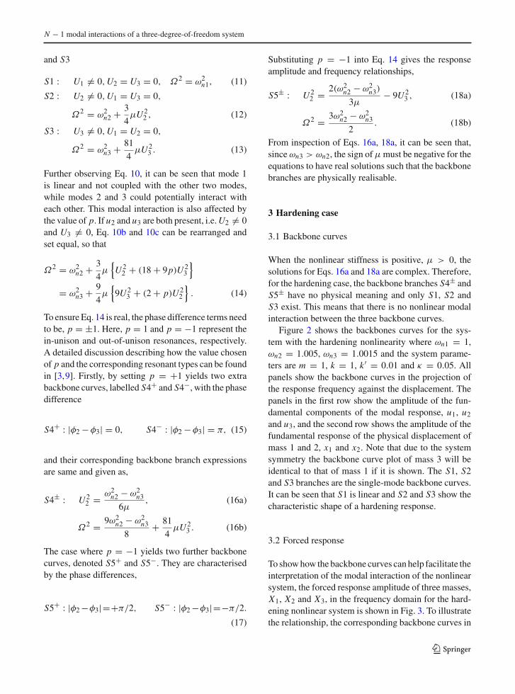
Figure 2 shows the backbones curves for the sys-tem with the hardening nonlinearity where ωn1 = 1,ωn2 = 1.005, ωn3 = 1.0015 and the system parame-ters are m = 1, k = 1, k′ = 0.01 and κ = 0.05. Allpanels show the backbone curves in the projection ofthe response frequency against the displacement. Thepanels in the first row show the amplitude of the fun-damental components of the modal response, u1, u2and u3, and the second row shows the amplitude of thefundamental response of the physical displacement ofmass 1 and 2, x1 and x2. Note that due to the systemsymmetry the backbone curve plot of mass 3 will beidentical to that of mass 1 if it is shown. The S1, S2and S3 branches are the single-mode backbone curves.It can be seen that S1 is linear and S2 and S3 show thecharacteristic shape of a hardening response.
3.2 Forced response
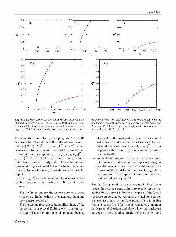
To showhow the backbone curves can help facilitate theinterpretation of the modal interaction of the nonlinearsystem, the forced response amplitude of three masses,X1, X2 and X3, in the frequency domain for the hard-ening nonlinear system is shown in Fig. 3. To illustratethe relationship, the corresponding backbone curves in
123
X. Liu et al.
1 1.01 1.02 1.030
0.2
0.4
0.6
0.8
Ω
U1
S1
3S2S
(a)
1 1.01 1.02 1.030
0.2
0.4
0.6
0.8
Ω
U2
S2
S3
(b)
1 1.01 1.02 1.030
0.2
0.4
0.6
0.8
Ω
U3
S2
S3
(c)
1 1.005 1.01 1.015 1.02 1.025 1.03 1.0350
0.1
0.2
0.3
0.4
0.5
0.6
0.7
0.8
Ω
X 1 S1 S2
S3
(d)
1 1.005 1.01 1.015 1.02 1.025 1.03 1.0350
0.1
0.2
0.3
0.4
0.5
0.6
0.7
0.8
Ω
X 2 S1
S2
S3
(e)
Fig. 2 Backbone curves for the nonlinear oscillator with thephysical parameters m = 1, k = 1, k′ = 0.01 and κ = 0.05,so the modal natural frequencies are ωn1 = 1, ωn2 = 1.005 andωn3 = 1.015. The panels in the first row show the modal dis-
placement results, Ui , and those of the second row represent thebackbone curve of the physical displacements of the mass 1 and2, X1 and X2. The corresponding single-mode backbone curvesare labelled by S1, S2 and S3
Fig. 2 are also shown. Here, a damping ratio ζ � 0.001is chosen for all modes and the external force ampli-tude is [P1, P2, P3]T = [3,−1, 1]T × 10−3, whichcorresponds to the situation where all three modes areexcited at the same amplitude, i.e. [Pm1, Pm2, Pm3]T =[1, 1, 1]T × 10−3. The forced response has been com-puted from an initial steady state solution, found withnumerical integration in MATLAB, which is then con-tinued in forcing frequency using the software AUTO-07p [4].
From Fig. 3, it can be seen that the response curvecan be divided into three parts from left to right by twominima,
– For the first resonance, the response curves of threemasses are similar to that of the linear oscillator andare centred around S1.
– For the second resonance, the familiar shape of theresponses of a typical Duffing oscillator are fol-lowing S2 and the jump phenomenon can be also
observed on the right part of the curve for mass 1and 3. Note that due to the special values of the lin-ear modeshape of mode 2, i.e. {1, 0,−1}T , there isno peak for the response of mass 2 in Fig. 3b withinthis bandwidth.
– For the third resonance, in Fig. 3a, the curve aroundS3 contains a loop where the upper trajectory isunstable which occurs from the addition and sub-traction of the modal contributions. In Fig. 3b, c,the response of the typical Duffing oscillator canbe observed enveloping S3.
For the first part of the response, mode 1 or linearmode, the resonant peak points are exactly on the lin-ear backbone curve S1. For the other parts of the forcedresponse curves, the curves cross the backbone curvesS2 and S3 almost at the fold points. This is in linewith the results found for systems with a lower numberof degrees of freedom and shows how the backbonecurves provide a good estimation of the position and
123
N − 1 modal interactions of a three-degree-of-freedom system
Fig. 3 Displacementamplitude of the threemasses when the system isforced by the external force[P1, P2, P3] =[3, −1, 1] × 10−3,corresponding to the modalforce [Pm1, Pm2, Pm3] =[1, 1, 1] × 10−3, withsystem parameters m = 1,k = 1, k′ = 0.01, κ = 0.05,c = 0.002 and c′ = 0. Theblue solid lines and reddashed lines represent thestable and unstableresponse, respectively. Thegrey lines representbackbone curves and the redstars represent fold points.(Color figure online)
0.98 1 1.02 1.04 1.06 1.08 1.1 1.120
0.1
0.2
0.3
0.4
0.5
0.6
0.7
0.8
0.9
Ω
X 1
(a)
0.98 1 1.02 1.04 1.06 1.08 1.1 1.120
0.1
0.2
0.3
0.4
0.5
0.6
0.7
0.8
0.9
Ω
X 2
(b)
0.98 1 1.02 1.04 1.06 1.08 1.1 1.120
0.1
0.2
0.3
0.4
0.5
0.6
0.7
0.8
0.9
Ω
X 3
(c)
the shape of resonant peaks in the frequency amplitudeplane.
4 Softening case
4.1 Backbone curves
For the softening case, μ < 0, Eqs. 16a and 18a havereal solutions. Therefore, the in-unison, S4±, and out-of-unison, S5±, resonant backbone curves are physi-
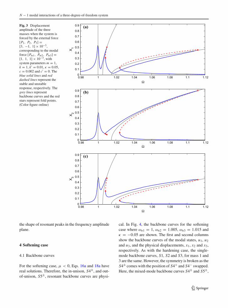
cal. In Fig. 4, the backbone curves for the softeningcase where ωn1 = 1, ωn2 = 1.005, ωn3 = 1.015 andκ = −0.05 are shown. The first and second columnsshow the backbone curves of the modal states, u1, u2and u3, and the physical displacements, x1, x2 and x3,respectively. As with the hardening case, the single-mode backbone curves, S1, S2 and S3, for mass 1 and3 are the same. However, the symmetry is broken as theS4± comes with the position of S4+ and S4− swapped.Here, the mixed-mode backbone curves S4± and S5±,
123

X. Liu et al.
where both mode 2 and 3 are activated, are of primaryinterest.
In Fig. 4, as expected the branch S1 is still a straightvertical line and S2 and S3 are curved, but with anopposite bending direction compared with those of thehardening system. Furthermore, it can be seen thatS4± emanate from branch S2 and S5± bifurcate frombranch S3. This type of bifurcation phenomenon hasbeen previously studied in other systems, see for exam-ple [3,9]. A significant difference from the previoussystems in the literature is that the S5± here is a ver-tical straight backbone curve which means that, likea linear mode, the resonant frequencies will not varywith the response amplitude. Also the backbone curveS5± has a finite length and it ends at S2, which impliesthat the out-of-unison resonance only happens withina certain amplitude range for this example.
4.2 Stability of the backbone curve
We now consider the stability of the backbone curves.Here, only the stability analysis of the backbone branchS2 is given in detail due to the fact that both S4± andS5± intersect with it, as shown in Fig. 4. Note that onbackbone curve S2 which is the solution of Eq. 12,u3 is equal to zero. So the stability of S2 can be deter-mined by considering the dynamics of u3 about its zerosolution (Note that u1 is not considered here due to itsindependence of u2 and u3). When the zero solution ofu3 is unstable, the S2 solution is also unstable.
Now, the unforced, undamped equation of mode 3,Eq. 8c, is consideredwith setting cm3 = 0 and Pm3 = 0,such that,
u3 + ω2n3u3 + 9μ[
2u2pu2mu3 +(u22pu3m + u22mu3p
)]= 0. (19)
As u3 is considered around its zero solution, theu3pu3mu3 term is so small that it has been neglected.The stability of the system is found by considering theamplitude and phase of u3 to be a slowly varying func-tions of time using the parameter ε to denote ’small-ness’. A similar treatment can also be seen in [28].Combined with ui = uip + uim , we can write u3 as
u3 = u3p + u3m = U3p(εt)
2e jωr3t + U3m(εt)
2e− jωr3t .
(20)
Furthermore, the derivatives of u3 can be written as,
u3 = jωr3
(U3p(εt)
2e jωr3t − U3m(εt)
2e− jωr3t
)
+ ε
(U3p(εt)
2e jωr3t + U3m(εt)
2e− jωr3t
),
(21)
and
u3 = −ω2r3u3
+ 2 jωr3ε
(U3p(εt)
2e jωr3t − U3m(εt)
2e− jωr3t
)
+O(ε2), (22)
where order ε2 terms have been neglected. Substitutingthe expression of u3 into Eq. 19 and then balancing thecoefficients of the e jωr3t and e− jωr3t terms gives,
U3p = − j
(ω2r3 − ω2
n3
ωr3
)U3p
2
+ j9μ
8ωr3
(2U2pU2mU3p +U 2
2pU3m
),
(23a)
and
U3m = j
(ω2r3 − ω2
n3
ωr3
)U3m
2
− j9μ
8ωr3
(2U2pU2mU3m +U 2
2mU3p
).
(23b)
Now these equations can be expressed in the form,
U3 = fU3U3, (24)
where U3 = {U3p U3m}T and the Jacobian matrix is,
fU3 = j
ωr3⎡⎣
9μ4 U2pU2m − ω2
r3−ω2n3
29μ8 U 2
2p
− 9μ8 U 2
2m − 9μ4 U2pU2m + ω2
r3−ω2n3
2
⎤⎦ .
So the stability of the zero solution ofu3 canbe assessedby considering the eigenvalues of thematrix, fU3 , aboutthe equilibrium solution U3 = 0. So, the eigenvalues,
123

N − 1 modal interactions of a three-degree-of-freedom system
0.96 0.97 0.98 0.99 1 1.010
0.1
0.2
0.3
0.4
0.5
0.6
0.7
0.8
S1
3S2SS4± BP1BP2,3
U1
Ω
(a)
0.96 0.97 0.98 0.99 1 1.010
0.1
0.2
0.3
0.4
0.5
0.6
0.7
0.8
S1
S2
S3
S4+
S4−
S5±
BP1
BP2
BP3
X 1
Ω
(b)
0.96 0.97 0.98 0.99 1 1.010
0.1
0.2
0.3
0.4
0.5
0.6
0.7
0.8
S2
S3
S4±
S5±
BP1
BP2
BP3
U2
Ω
(c)
0.96 0.97 0.98 0.99 1 1.010
0.1
0.2
0.3
0.4
0.5
0.6
0.7
0.8
S1
S2
S3
S4± S5±
BP1
BP3
BP2
X 2
Ω
(d)
0.96 0.97 0.98 0.99 1 1.010
0.1
0.2
0.3
0.4
0.5
0.6
0.7
0.8
S2
S3
S4±
S5±
BP1BP2
BP3
U3
Ω
(e)
0.96 0.97 0.98 0.99 1 1.010
0.1
0.2
0.3
0.4
0.5
0.6
0.7
0.8
S1
S2
S3
S4−
S4+
S5±
BP1
BP2
BP3
X 3
Ω
(f)
Fig. 4 Backbone curves for the oscillator with the physical para-meters k = 1, k′ = 0.01 and κ = −0.05, such that the modalnatural frequencies are ωn1 = 1, ωn2 = 1.005 and ωn3 = 1.015.The panels in the first and second column show the modal andphysical displacement results, respectively. Stable solutions are
shown with the solid lines, whereas unstable solutions are repre-sented by the dashed lines. Bifurcation points are noted by BPi .Note that due to the identical natural frequencies, the branchesS5± overlap with S1, so the S5± backbone curves are indicatedby the short cross lines for distinction
123

X. Liu et al.
λ, are given by,
ω2r3λ
2 +(9μ
4U 22 − ω2
r3 − ω2n3
2
)2
−(9μ
8U 22
)2
= 0,
(25)
where U 22 = U2pU2m has been used. From inspecting
the above equation, it can be seen that the values of λ
can be only be either purely imaginary or real. Whenall the eigenvalues, λ, are purely imaginary the systemis marginally stable, while when λ are real the systemis unstable. This implies that the bifurcation point onthe backbone curve occurs when both of the roots ofEq. 25 are zero, such that,
∣∣∣∣∣9μ
4U 22 − ω2
r3 − ω2n3
2
∣∣∣∣∣ =∣∣∣∣9μ
8U 22
∣∣∣∣ . (26)
Then using the expression for S2 given in Eq. 12 givesthe bifurcation points,
BP1 : Ω2 = 9ω2n2 − ω2
n3
8& U 2
2 = ω2n2 − ω2
n3
6μ, (27)
and
BP2 : Ω2 = 3ω2n2 − ω2
n3
2& U 2
2 = 2(ω2n2 − ω2
n3)
3μ.
(28)
These are the same points where S4± and S5± inter-sect with S2, respectively. Note that since the linearnatural frequencies of the modes are similar, the res-onant response of the second and third modes will beat the same frequency. Hence, here, the relationshipωr3 = ωr2 = Ω has been used to simplify the equa-tions.
Using the same approach, it can be also shown thatthe parts of S2 below bifurcation point BP1 and aboveBP2 are stable and the part between the two bifurcationpoints is unstable.
The same method was also used to predict that onS3 there is another bifurcation point,
BP3 : Ω2 = 3ω2n2 − ω2
n3
2& U 2
3 = 2(ω2n2 − ω2
n3)
27μ,
(29)
which is the intersection point of S3 and S5±. Also thestability condition of branch S3 is that the part belowBP3 is stable and the section above is unstable.All thesebifurcation points are also shown in Fig. 4. Using bifur-cation theory for Hamiltonian systems and comparingwith other similar systems in the published literature,all the bifurcation points here are (Hamiltonian) pitch-fork bifurcations [3,7,25].
4.3 Analysis of the forced response
4.3.1 Forced response
We now examine the relationship between the forcedresponse and the backbone curves for the softeningnonlinear case. From the backbone curve results, itcan be seen that the modal interactions occur for thiscase. Therefore, a simple forced configuration whereonly mode 2 is excited is chosen as two kinds ofinteractions bifurcate from backbone curve S2. Forthis forcing configuration, three different force ampli-tudes are chosen which are [Pm1, Pm2, Pm3] =[0, 0.4, 0]×10−3, [0, 0.9, 0]×10−3 and [0, 1.5, 0]×10−3 and the damping ratio is chosen to be ζ =0.001.
Figure 5 shows the forced response results superim-posed on the backbone curves for mass 1.
– For the small force amplitude situation, Fig. 5a,there is only one response curve which is centredaround S2. This curve is the response of a typicalsoftening Duffing oscillator and only composed theresponse of mode 2, u2. For this case, the forceis insufficient to trigger the modal interaction orjump.
– For the medium force amplitude situation, Fig. 5b,there are three response curves (1 blue and 2 green).The two green curves following S4± bifurcate fromthe single-mode response curve (blue one) at twosecondary bifurcation points, respectively, and theyare composed of the response of both mode 2, u2,and mode 3, u3.
– For the large force amplitude situation, Fig. 5c,there are two additional response curves (the blackones) surrounding S5± which also bifurcates fromthe single-mode response curve ofmode2.On thesetwo curves, both mode 2 and 3 are present as well.
From the results in Fig. 5, it can be noticed that forthe situation where only one nonlinear mode is directly
123
N − 1 modal interactions of a three-degree-of-freedom system
0.98 0.985 0.99 0.995 1 1.005 1.01 1.015 1.020
0.1
0.2
0.3
0.4
0.5
0.6
0.7
0.8
Ω
X 1(a)
0.98 0.985 0.99 0.995 1 1.005 1.01 1.015 1.020
0.1
0.2
0.3
0.4
0.5
0.6
0.7
0.8
Ω
X 1
(b)
0.98 0.985 0.99 0.995 1 1.005 1.01 1.015 1.020
0.1
0.2
0.3
0.4
0.5
0.6
0.7
0.8
Ω
X 1
(c)
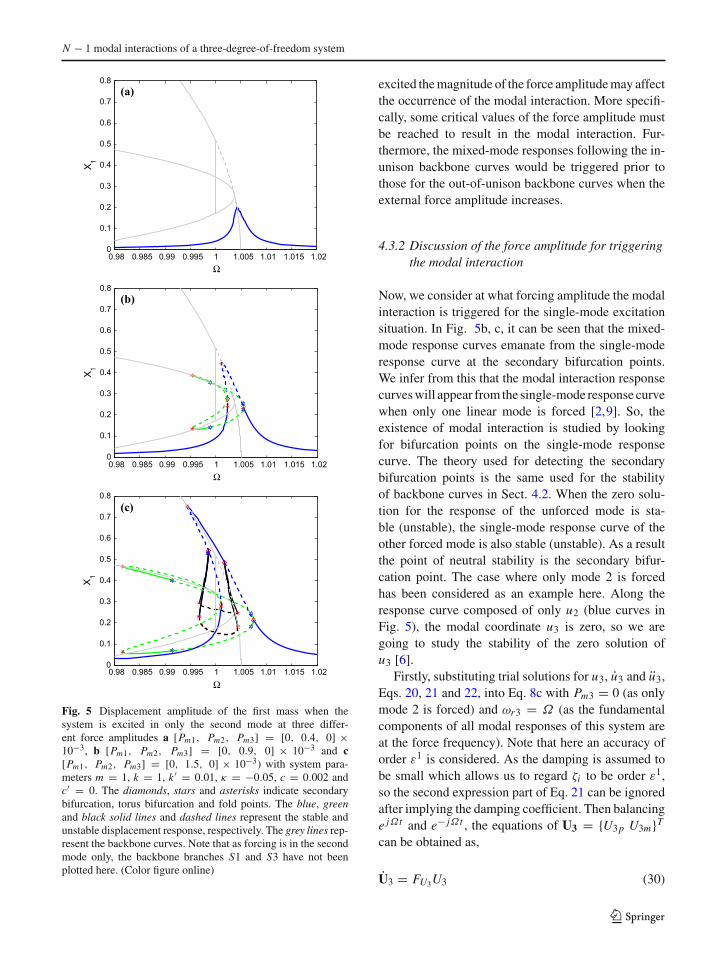
Fig. 5 Displacement amplitude of the first mass when thesystem is excited in only the second mode at three differ-ent force amplitudes a [Pm1, Pm2, Pm3] = [0, 0.4, 0] ×10−3, b [Pm1, Pm2, Pm3] = [0, 0.9, 0] × 10−3 and c[Pm1, Pm2, Pm3] = [0, 1.5, 0] × 10−3) with system para-meters m = 1, k = 1, k′ = 0.01, κ = −0.05, c = 0.002 andc′ = 0. The diamonds, stars and asterisks indicate secondarybifurcation, torus bifurcation and fold points. The blue, greenand black solid lines and dashed lines represent the stable andunstable displacement response, respectively. The grey lines rep-resent the backbone curves. Note that as forcing is in the secondmode only, the backbone branches S1 and S3 have not beenplotted here. (Color figure online)
excited themagnitude of the force amplitudemay affectthe occurrence of the modal interaction. More specifi-cally, some critical values of the force amplitude mustbe reached to result in the modal interaction. Fur-thermore, the mixed-mode responses following the in-unison backbone curves would be triggered prior tothose for the out-of-unison backbone curves when theexternal force amplitude increases.
4.3.2 Discussion of the force amplitude for triggeringthe modal interaction
Now, we consider at what forcing amplitude the modalinteraction is triggered for the single-mode excitationsituation. In Fig. 5b, c, it can be seen that the mixed-mode response curves emanate from the single-moderesponse curve at the secondary bifurcation points.We infer from this that the modal interaction responsecurveswill appear from the single-mode response curvewhen only one linear mode is forced [2,9]. So, theexistence of modal interaction is studied by lookingfor bifurcation points on the single-mode responsecurve. The theory used for detecting the secondarybifurcation points is the same used for the stabilityof backbone curves in Sect. 4.2. When the zero solu-tion for the response of the unforced mode is sta-ble (unstable), the single-mode response curve of theother forced mode is also stable (unstable). As a resultthe point of neutral stability is the secondary bifur-cation point. The case where only mode 2 is forcedhas been considered as an example here. Along theresponse curve composed of only u2 (blue curves inFig. 5), the modal coordinate u3 is zero, so we aregoing to study the stability of the zero solution ofu3 [6].
Firstly, substituting trial solutions for u3, u3 and u3,Eqs. 20, 21 and 22, into Eq. 8c with Pm3 = 0 (as onlymode 2 is forced) and ωr3 = Ω (as the fundamentalcomponents of all modal responses of this system areat the force frequency). Note that here an accuracy oforder ε1 is considered. As the damping is assumed tobe small which allows us to regard ζi to be order ε1,so the second expression part of Eq. 21 can be ignoredafter implying the damping coefficient. Then balancinge jΩt and e− jΩt , the equations of U3 = {U3p U3m}Tcan be obtained as,
U3 = FU3U3 (30)
123
X. Liu et al.
where
FU3 =
⎡⎢⎢⎣
Ω2−ω2n3− 9μ
2 U2pU2m− j2ωn3ζ3Ω
2 jΩ − 9μU22p
8 jΩ
9μU22m
8 jΩΩ2−ω2
n3− 9μ2 U2pU2m+ j2ωn3ζ3Ω
−2 jΩ
⎤⎥⎥⎦ .
Then the eigenvalues , λ, for FU3 can be obtained from,
aλ2 + bλ + c = 0, (31)
where
a = 4Ω2,
b = 8ωn3ζ3Ω2,
and
c = (Ω2 − ω2n3)
2 − 9μU 22 (Ω2 − ω2
n3)
+ 243
16U 42 + (2ωn3ζ3Ω)2.
Therefore, the stability of the zero solution, U3 = 0,can be determined from the eigenvalues, λi , i = 1, 2.The roots of Eq. 31 are given by,
λ1,2 = −b ±√
(b2 − 4ac)
2a. (32)
For all parameter values in this example a and b arepositive. So when one of the eigenvalues is zero andanother is negative real, the system is neutrally stable.Therefore, the bifurcation occurs when c is zero, suchthat,
243μ2U 42 − 144μ(Ω2 − ω2
n3)U22
+16[(Ω2 − ω2
n3)2 + (2ωn3ζ3Ω)2
]= 0.
(33)
Combining Eq. 33 with the equation for the single-mode response curve for u2 obtained by settingU3 = 0in Eq. 8(b) expressed as below,
9μ2U 62 + 24μ(ω2
n2 − Ω2)U 42
+16[(ω2
n2 − Ω2)2 + (2ωn2ζ2Ω)2]U 22 = 16P2
m2,
(34)
it allows us to find the position and number of theirintersection points. To ensure the solutions are physi-cally reasonable, only the intersection points at U > 0
and Ω > 0 are considered. Those points are secondarybifurcation points that can be used to predict the onsetof the modal interaction.
There are three possible cases:
(1) if there is zero or one intersection point, there willbe no modal interaction. Fig. 6a.
(2) if there are two or three intersection points, themodal interaction response following the in-unisonbackbone curves will exist. Fig. 6b.
(3) if there are four intersection points, both the modalinteraction response following the in-unison andout-of-unison backbone curves will occur. Fig-ure 6c.
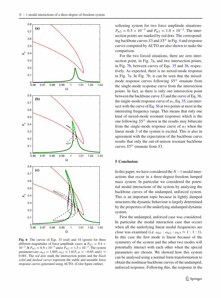
Figure 6 shows the curves of Eqs. 33 (red) and 34(green) with the same parameter values of the sys-tem shown in Fig. 5, and their intersection points aremarked by red dots. To make a comparison, the cor-responding response curves (black) in Fig. 5 are alsoshown here. From Fig. 6, it can be seen that the single-mode response curve results approximated using thenormal form technique and those calculated by AUTOare in good agreement. In addition, the intersections ofEqs. 33 and 34 are very close to the secondary bifur-cation points for every case. The results show that theanalyticalmethodpresented in this paper can be appliedto detect the occurrence of modal interaction and iden-tify the position of bifurcation points.
Furthermore, when only mode 3 is excited, the sameanalysis method can be applied to find the bifurcationpoints at the single-mode response curve composed ofonly u3. This leads to two equations below,
2187μ2U 43 − 432μ(Ω2 − ω2
n2)U23
+16[(Ω2 − ω2
n2)2 + (2ωn2ζ2Ω)2
]= 0,
(35)
and
6561μ2U 63 + 648μ(ω2
n3 − Ω2)U 43
+16[(ω2
n3 − Ω2)2 + (2ωn3ζ3Ω)2]U 23 = 16P2
m3.
(36)
Similarly, combining Eqs. 35 and 36 to find the posi-tion and number of their intersection points, we canpredict the occurrence of modal interaction for theonly mode 3 forced situation. Figure 7 shows theposition relationship between these two curves of the
123
N − 1 modal interactions of a three-degree-of-freedom system
0.96 0.97 0.98 0.99 1 1.01 1.02 1.030
0.1
0.2
0.3
0.4
0.5
0.6
0.7
0.8
Ω
X 1(a)
0.96 0.97 0.98 0.99 1 1.01 1.02 1.030
0.1
0.2
0.3
0.4
0.5
0.6
0.7
0.8
Ω
X 1
(b)
0.96 0.97 0.98 0.99 1 1.01 1.02 1.030
0.1
0.2
0.3
0.4
0.5
0.6
0.7
0.8
Ω
X 1
(c)
Fig. 6 The curves of Eqs. 33 (red) and 34 (green) for threedifferent magnitudes of force amplitude cases: a Pm2 = 0.4 ×10⁻³, b Pm2 = 0.9×10⁻³ and c Pm2 = 1.5×10⁻³. The systemparameters are:ωn2 = 1.005,ωn3 = 1.015,μ = −0.05, and ζ ≈0.001. The red dots mark the intersection points and the blacksolid and dashed curves represent the stable and unstable forceresponse curves generated using AUTO. (Color figure online)
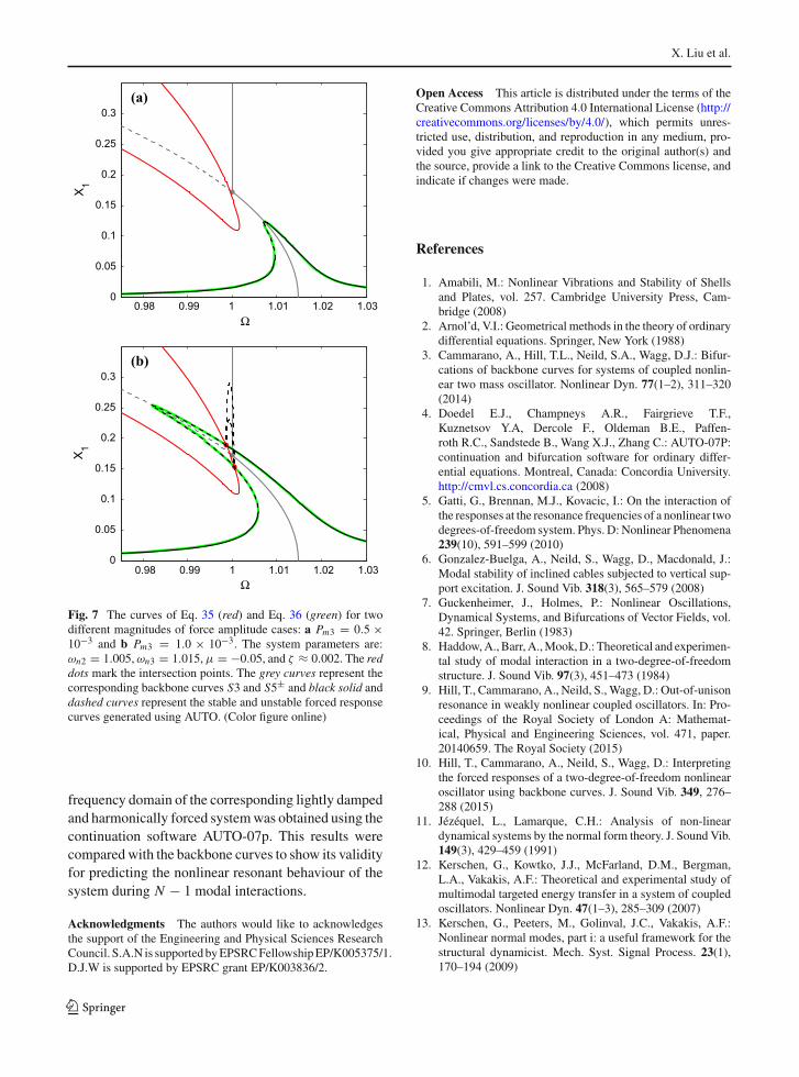
softening system for two force amplitude situations:Pm3 = 0.5 × 10⁻³ and Pm3 = 1.0 × 10⁻³. The inter-section points are marked by red dots. The correspond-ing backbone curves S3 and S5± in Fig. 4 and responsecurves computed by AUTO are also shown to make thecomparison.
For the two forced situations, there are zero inter-section point, in Fig. 7a, and two intersection points,in Fig. 7b, between curves of Eqs. 35 and 36, respec-tively. As expected, there is no mixed-mode responsein Fig. 7a. In Fig. 7b, it can be seen that the mixed-mode response curves following S5± emanate fromthe single-mode response curve from the intersectionpoints. In fact, as there is only one intersection pointbetween the backbone curve S3 and the curve of Eq. 36,the single-mode response curve of u3, Eq. 35, can inter-sect with the curve of Eq. 36 at two points at most in theinteresting frequency range. This means that only onekind of mixed-mode resonant responses which is theone following S5± shown in the results may bifurcatefrom the single-mode response curve of u3 when thelinear mode 3 of the system is excited. This is also inagreement with the expectation of the backbone curveresults that only the out-of-unison resonant backbonecurves S5± emanate from S3.
5 Conclusion
In this paper, we have considered the N−1modal inter-actions that occur in a three-degree-freedom lumpedmass system. In particular we considered the poten-tial modal interactions of the system by analysing thebackbone curves of the undamped, unforced system.This is an important topic because in lightly dampedstructures the dynamic behaviour is largely determinedby the properties of the underlying undamped dynamicsystem.
First the undamped, unforced case was considered.In particular the modal interaction case that occurswhen all the underlying linear modal frequencies areclose was examined (i.e. ωn1 : ωn2 : ωn3 ≈ 1 : 1 : 1).In this case the first mode is linear because of thesymmetry of the system and the other two modes willpotentially interact with each other when the specialparameters are chosen. We showed how this systemcan be analysed using a normal form transformation toobtain the nonlinear backbone curves of the undamped,unforced response. Following this, the response in the
123
X. Liu et al.
0.98 0.99 1 1.01 1.02 1.030
0.05
0.1
0.15
0.2
0.25
0.3
Ω
X 1(a)
0.98 0.99 1 1.01 1.02 1.030
0.05
0.1
0.15
0.2
0.25
0.3
Ω
X 1
(b)
Fig. 7 The curves of Eq. 35 (red) and Eq. 36 (green) for twodifferent magnitudes of force amplitude cases: a Pm3 = 0.5 ×10⁻³ and b Pm3 = 1.0 × 10⁻³. The system parameters are:ωn2 = 1.005,ωn3 = 1.015,μ = −0.05, and ζ ≈ 0.002. The reddots mark the intersection points. The grey curves represent thecorresponding backbone curves S3 and S5± and black solid anddashed curves represent the stable and unstable forced responsecurves generated using AUTO. (Color figure online)
frequency domain of the corresponding lightly dampedand harmonically forced systemwas obtained using thecontinuation software AUTO-07p. This results werecompared with the backbone curves to show its validityfor predicting the nonlinear resonant behaviour of thesystem during N − 1 modal interactions.
Acknowledgments The authors would like to acknowledgesthe support of the Engineering and Physical Sciences ResearchCouncil. S.A.N is supportedbyEPSRCFellowshipEP/K005375/1.D.J.W is supported by EPSRC grant EP/K003836/2.
Open Access This article is distributed under the terms of theCreative Commons Attribution 4.0 International License (http://creativecommons.org/licenses/by/4.0/), which permits unres-tricted use, distribution, and reproduction in any medium, pro-vided you give appropriate credit to the original author(s) andthe source, provide a link to the Creative Commons license, andindicate if changes were made.
References
1. Amabili, M.: Nonlinear Vibrations and Stability of Shellsand Plates, vol. 257. Cambridge University Press, Cam-bridge (2008)
2. Arnol’d, V.I.: Geometrical methods in the theory of ordinarydifferential equations. Springer, New York (1988)
3. Cammarano, A., Hill, T.L., Neild, S.A., Wagg, D.J.: Bifur-cations of backbone curves for systems of coupled nonlin-ear two mass oscillator. Nonlinear Dyn. 77(1–2), 311–320(2014)
4. Doedel E.J., Champneys A.R., Fairgrieve T.F.,Kuznetsov Y.A, Dercole F., Oldeman B.E., Paffen-roth R.C., Sandstede B., Wang X.J., Zhang C.: AUTO-07P:continuation and bifurcation software for ordinary differ-ential equations. Montreal, Canada: Concordia University.http://cmvl.cs.concordia.ca (2008)
5. Gatti, G., Brennan, M.J., Kovacic, I.: On the interaction ofthe responses at the resonance frequencies of a nonlinear twodegrees-of-freedom system. Phys. D: Nonlinear Phenomena239(10), 591–599 (2010)
6. Gonzalez-Buelga, A., Neild, S., Wagg, D., Macdonald, J.:Modal stability of inclined cables subjected to vertical sup-port excitation. J. Sound Vib. 318(3), 565–579 (2008)
7. Guckenheimer, J., Holmes, P.: Nonlinear Oscillations,Dynamical Systems, and Bifurcations of Vector Fields, vol.42. Springer, Berlin (1983)
8. Haddow,A., Barr,A.,Mook,D.: Theoretical and experimen-tal study of modal interaction in a two-degree-of-freedomstructure. J. Sound Vib. 97(3), 451–473 (1984)
9. Hill, T., Cammarano, A., Neild, S.,Wagg, D.: Out-of-unisonresonance in weakly nonlinear coupled oscillators. In: Pro-ceedings of the Royal Society of London A: Mathemat-ical, Physical and Engineering Sciences, vol. 471, paper.20140659. The Royal Society (2015)
10. Hill, T., Cammarano, A., Neild, S., Wagg, D.: Interpretingthe forced responses of a two-degree-of-freedom nonlinearoscillator using backbone curves. J. Sound Vib. 349, 276–288 (2015)
11. Jézéquel, L., Lamarque, C.H.: Analysis of non-lineardynamical systems by the normal form theory. J. Sound Vib.149(3), 429–459 (1991)
12. Kerschen, G., Kowtko, J.J., McFarland, D.M., Bergman,L.A., Vakakis, A.F.: Theoretical and experimental study ofmultimodal targeted energy transfer in a system of coupledoscillators. Nonlinear Dyn. 47(1–3), 285–309 (2007)
13. Kerschen, G., Peeters, M., Golinval, J.C., Vakakis, A.F.:Nonlinear normal modes, part i: a useful framework for thestructural dynamicist. Mech. Syst. Signal Process. 23(1),170–194 (2009)
123
N − 1 modal interactions of a three-degree-of-freedom system
14. Lamarque, C.H., Touzé, C., Thomas, O.: An upper boundfor validity limits of asymptotic analytical approaches basedon normal form theory. Nonlinear Dyn. 70(3), 1931–1949(2012)
15. Lewandowski, R.: On beams membranes and plates vibra-tion backbone curves in cases of internal resonance. Mec-canica 31(3), 323–346 (1996)
16. Nayfeh, A.H.: Nonlinear Interactions. Wiley, Hoboken(2000)
17. Nayfeh, A.H., Balachandran, B.: Modal interactions indynamical and structural systems. Appl. Mech. Rev.42(11S), S175–S201 (1989)
18. Nayfeh, A.H., Mook, D.T.: Nonlinear Oscillations. Wiley,Hoboken (2008)
19. Nayfeh, A.H., Pai, P.F.: Linear and Nonlinear StructuralMechanics. Wiley, Hoboken (2008)
20. Neild, S., Wagg, D.: A generalized frequency detuningmethod for multidegree-of-freedom oscillators with nonlin-ear stiffness. Nonlinear Dyn. 73(1–2), 649–663 (2013)
21. Neild, S.A., Wagg, D.J.: Applying the method of normalforms to second-order nonlinear vibration problems. Proc.R. Soc A: Math., Phys. Eng. Sci. 467(2128), 1141–1163(2011)
22. Pierre, C., Jiang, D., Shaw, S.: Nonlinear normal modes andtheir application in structural dynamics. Math. Probl. Eng.2006, 1–15 (2006)
23. Rand, R.H.: Nonlinear normal modes in two-degree-of-freedom systems. J. Appl. Mech. 38(2), 561–561 (1971)
24. Rega, G., Lacarbonara, W., Nayfeh, A., Chin, C.: Multipleresonances in suspended cables: direct versus reduced-ordermodels. Int. J. Non-Linear Mech. 34(5), 901–924 (1999)
25. Thompson, J.M.T., Stewart, H.B.: Nonlinear Dynamics andChaos. Wiley, Hoboken (2002)
26. Touzé, C., Amabili, M.: Nonlinear normal modes fordamped geometrically nonlinear systems: application toreduced-order modelling of harmonically forced structures.J. Sound Vib. 298(4), 958–981 (2006)
27. Touzé, C., Thomas, O., Chaigne, A.: Asymmetric non-linearforced vibrations of free-edge circular plates. part 1: theory.J. Sound Vib. 258(4), 649–676 (2002)
28. Wagg, D., Neild, S.: Nonlinear Vibration with Control: forFlexible and Adaptive Structures, vol. 218. Springer, Berlin(2014)
29. Xin, Z., Neild, S., Wagg, D., Zuo, Z.: Resonant responsefunctions for nonlinear oscillators with polynomial typenonlinearities. J. Sound Vib. 332(7), 1777–1788 (2013)
123