model-based analysis of sensor-noise in predictive passive ... · model-based analysis of...

MODEL-BASED ANALYSIS OFSENSOR-NOISE IN PREDICTIVE PASSIVE SAFETY ALGORITHMS

Tobias DirndorferRobotics and Embedded Systems, Technische Universitat MunchenMichael BotschDepartment for Active and Passive Safety, AUDI AG, IngolstadtAlois KnollRobotics and Embedded Systems, Technische Universitat MunchenGermanyPaper Number 11-0251

ABSTRACT

The introduction of environment perception sensorsinto the automotive world enables further improve-ment of the already highly optimized passive safetysystems. Such sensors facilitate the development ofsafety applications that can act in a context sen-sitive manner concerning the protection of vehicleoccupants. Hereby the quality of the provided in-formation is decisive for the usability and effectiverange of such sensors within integrated safety sys-tems. In this paper noise effects in sensors and theirimplications on the prediction of collision parame-ters are analyzed. The focus lies on sensors thatcan measure distances but not velocities or acceler-ations of the objects surrounding the car. For suchsensors a noise model is presented as well as a track-ing algorithm aiming to estimate the velocities andto compensate the effects of noise. This informationis used by a trajectory-based algorithm to predictrelevant collision parameters like time-to-collision,relative velocity at collision time etc. Monte Carlosimulations show the influence of noise on the ac-curacy of the predicted collision parameters. Thedescribed model-based study allows the systematicdeduction of sensor requirements and represents anew way for the evaluation of the robustness of pre-dictive passive safety systems.

INTRODUCTION

Modern cars provide a high level of safety dueto the optimization of bodywork, seat-belts orairbags in the last decades. Conventional pas-sive safety applications for the activation of oc-cupant restraint systems work on established sen-sor concepts, e.g., acceleration and pressure sen-sors, and have already reached a high level of adap-tivity and robustness. The introduction of envi-ronment perception sensors leads to a further im-provement of security, since safety systems can bedeveloped that act in a context sensitive man-ner [1, 2, 3, 4]. First applications like the proac-tive reversible belt-tensioner can already be foundin new cars, e. g., in the Audi A7 [5], and the adap-

tation of airbags and other passive safety systemsto the specific crash situation are in the focus ofcurrent development. Future cars will combine allavailable information—including those gained byCar-to-X (http://www.simTD.de, http://www.car-to-car.org) technologies—concerning the environ-ment to increase the effectiveness of vehicle safetyin an integral sense.The number of sensors that are and will be in-tegrated in new vehicles is increasing since appli-cations have various requirements concerning therange, aperture, sensitivity or other properties.Typical applications using such sensors are mainlylocated in the field of advanced driver assistancesystems like automatic cruise control, lane assist,heading control, etc. In the vehicle safety domainrequirements on such sensors are high, i. e., a verysmall false positive rate and a very high true pos-itive rate in the detection of objects in the envi-ronment of the car. Not only the detection of anobject’s existence is of high interest but also itsexact location, velocity and geometry. Such pre-crash information allows the estimation of collisionparameters before a collision occurs. This infor-mation can be used to optimize the activation ofadaptive restraint systems. However, the pre-crash-prediction of the collision parameters is subject toa couple of disturbance effects, e.g., inexact mea-surements as well as time delays caused by trackingalgorithms or the communication between differentelectronic control units. These factors can affect

Figure 1. Effects of sensor noise on the col-lision prediction

Dirndorfer, Botsch, Knoll 1

the required precision of predictive crash severityestimations and therefore the effectiveness of inte-grated safety systems. The example from Figure 1illustrates that a large noise power of the predic-tive sensor can lead to a wrong prediction of how ascenario will develop in the future. Assuming thatthe dynamic parameters like velocities or accelera-tions do not change during the prediction intervala small noise power disturbs the prediction mar-ginally, whereas a large noise power can lead to acompletely wrong estimation of the scenario. Thefirst illustration in Figure 1 shows a prediction withno measurement noise, the second illustration thesame scenario but under the assumption that smallnoise power disturbs the measurement and the thirdillustration the same scenario but under the as-sumption that a large noise power disturbs the mea-surement. Therefore, it is necessary to quantify theeffect of noise on predictions that are used to adaptrestraint systems by taking into account the wholesignal processing chain. This paper focuses on sucha model of disturbance effects and their influenceon the computation of relevant collision parameterslike the time-to-collision, the relative velocity at col-lision time, the collision angle and further geometricparameters. On the one hand the noise caused bysensors describing the state of the ego vehicle andon the other hand the noise caused by predictivesensors detecting the vehicle environment are con-sidered. Whereas a stationary white noise Gaussianrandom process is assumed for the noise disturb-ing the ego-state, for the predictive sensor a moresophisticated model is applied. The focus lies onsensors able to measure the position and geometryof objects but not their velocity and acceleration.The velocity must be estimated based on positionchanges which is accomplished here using a Kalmanfilter. Thus, the noise process describing the in-accuracy of the position measurement determinesthe noise process for the velocity. The model forposition inaccuracies takes into account a distancebased noise power. On the basis of such a noisemodel Monte Carlo simulations are performed forfour predictive sensor variants to analyze the ef-fects on the computed collision parameters. Thefour sensor variants were chosen to represent sen-sors with different performances.

The chapter “MEASUREMENT DATA” intro-duces the relative dynamics model and the sensornoise model that are used in the Monte Carlo sim-ulations later on. Chapter “COLLISISION PRE-DICTION ALGORITHM” focuses on the trackingmodel and on the trajectory-based prediction mod-ule used to calculate the collision parameters. InChapter “MONTE CARLO SIMULATION” threetraffic scenarios are analyzed in detail and the ef-

fects of noisy measurements are presented. Thegeneral outline of the paper is illustrated in Fig-ure 2.

Figure 2. Outline of the paper

Throughout the paper vectors and matrices are de-noted by lower and upper case bold letters. AM ×N zero matrix is dented by 0M×N .

MEASUREMENT DATA

In this chapter the model-based generation processof noisy measurements as input data for a collisionprediction algorithm is described. Firstly the two-dimensional relative dynamics model used for thesimulation of ideal sensor data concerning the egovehicle and an ego-mounted predictive sensor mea-suring relative position data is explained. After-wards the application of sensor noise to the simu-lated exact reference data is depicted.

Relative dynamics model

For the motion simulation of the ego and opponentvehicle in specific collision scenarios a nonlinear sin-gle track model with a Pacejka tire force approachas described in [6] was applied (see Figure 3). Thismodel offers a good two-dimensional description ofthe global vehicle movement in stationary as wellas dynamic driving scenarios disregarding effects ofpitch and roll. As only the global vehicle trajec-tory over ground and not the exact knowledge ofinternal system state variables such as wheel rota-


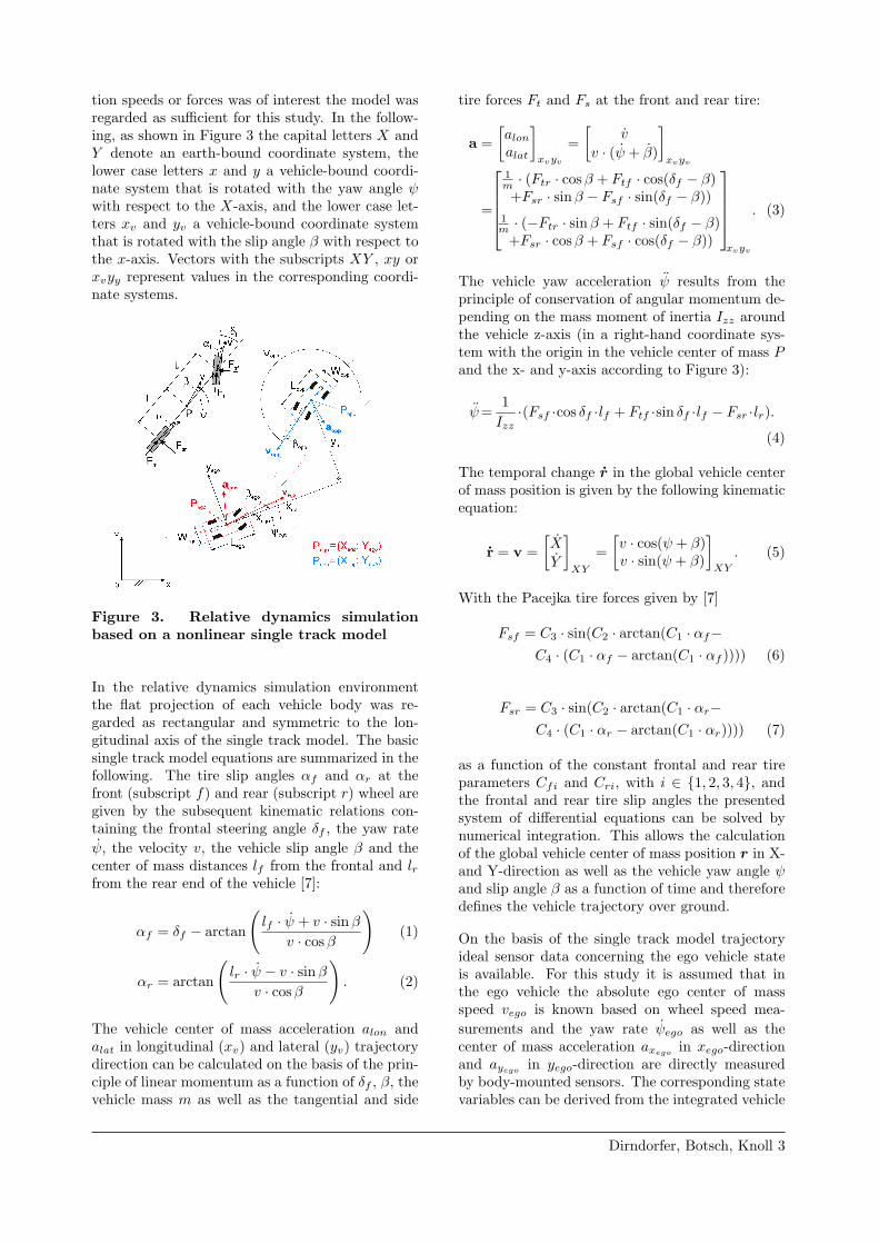
tion speeds or forces was of interest the model wasregarded as sufficient for this study. In the follow-ing, as shown in Figure 3 the capital letters X andY denote an earth-bound coordinate system, thelower case letters x and y a vehicle-bound coordi-nate system that is rotated with the yaw angle ψwith respect to the X-axis, and the lower case let-ters xv and yv a vehicle-bound coordinate systemthat is rotated with the slip angle β with respect tothe x-axis. Vectors with the subscripts XY , xy orxvyy represent values in the corresponding coordi-nate systems.

Figure 3. Relative dynamics simulationbased on a nonlinear single track model

In the relative dynamics simulation environmentthe flat projection of each vehicle body was re-garded as rectangular and symmetric to the lon-gitudinal axis of the single track model. The basicsingle track model equations are summarized in thefollowing. The tire slip angles αf and αr at thefront (subscript f) and rear (subscript r) wheel aregiven by the subsequent kinematic relations con-taining the frontal steering angle δf , the yaw rateψ, the velocity v, the vehicle slip angle β and thecenter of mass distances lf from the frontal and lrfrom the rear end of the vehicle [7]:

αf = δf − arctan

(lf · ψ + v · sinβ

v · cosβ

)(1)

αr = arctan

(lr · ψ − v · sinβ

v · cosβ

). (2)

The vehicle center of mass acceleration alon andalat in longitudinal (xv) and lateral (yv) trajectorydirection can be calculated on the basis of the prin-ciple of linear momentum as a function of δf , β, thevehicle mass m as well as the tangential and side

tire forces Ft and Fs at the front and rear tire:

a =[alonalat

]xvyv

=[

v

v · (ψ + β)

]xvyv

=

1m · (Ftr · cosβ + Ftf · cos(δf − β)+Fsr · sinβ − Fsf · sin(δf − β))

1m · (−Ftr · sinβ + Ftf · sin(δf − β)

+Fsr · cosβ + Fsf · cos(δf − β))

xvyv

. (3)

The vehicle yaw acceleration ψ results from theprinciple of conservation of angular momentum de-pending on the mass moment of inertia Izz aroundthe vehicle z-axis (in a right-hand coordinate sys-tem with the origin in the vehicle center of mass Pand the x- and y-axis according to Figure 3):

ψ=1Izz

·(Fsf ·cos δf ·lf + Ftf ·sin δf ·lf − Fsr ·lr).

(4)

The temporal change r in the global vehicle centerof mass position is given by the following kinematicequation:

r = v =[X

Y

]XY

=[v · cos(ψ + β)v · sin(ψ + β)

]XY

. (5)

With the Pacejka tire forces given by [7]

Fsf = C3 · sin(C2 · arctan(C1 · αf−C4 · (C1 · αf − arctan(C1 · αf )))) (6)

Fsr = C3 · sin(C2 · arctan(C1 · αr−C4 · (C1 · αr − arctan(C1 · αr)))) (7)

as a function of the constant frontal and rear tireparameters Cfi and Cri, with i ∈ {1, 2, 3, 4}, andthe frontal and rear tire slip angles the presentedsystem of differential equations can be solved bynumerical integration. This allows the calculationof the global vehicle center of mass position r in X-and Y-direction as well as the vehicle yaw angle ψand slip angle β as a function of time and thereforedefines the vehicle trajectory over ground.

On the basis of the single track model trajectoryideal sensor data concerning the ego vehicle stateis available. For this study it is assumed that inthe ego vehicle the absolute ego center of massspeed vego is known based on wheel speed mea-surements and the yaw rate ψego as well as thecenter of mass acceleration axego in xego-directionand ayego in yego-direction are directly measuredby body-mounted sensors. The corresponding statevariables can be derived from the integrated vehicle


trajectory via the following equations:

vego = |vego| =√X2ego + Y 2

ego (8)

ψego =dψegodt

(9)

axego= cos(βego) · vego− sin(βego) · vego · (ψego + βego) (10)

ayego = sin(βego) · vego+ cos(βego) · vego · (ψego + βego). (11)

The parallel simulation of two trajectories offers thepossibility to calculate the relative position datarPopp/Pego

measured by an ideal ego-mounted pre-dictive sensor which can be calculated for any givenreference point rPopp

on the opponent vehicle.

For a predictive sensor located at rPsensand

mounted at a displacement of xPsens/Pegoin xego-

direction and yPsens/Pegoin yego-direction relative

to the ego center of mass rPegothe relative location

measurement of the opponent reference point rPopp

is given by:[xsensysens

]xegoyego

:= rPopp/P sens= rPopp − rPsens =

=[XPopp

YPopp

]XY

−

[[XPego

YPego

]XY

+[xPsens/Pego

yPsens/Pego

]xegoyego

]

=

(XPopp

−XPego) cosψego

+(YPopp− Y Pego

) sinψego−xPsens/Pego

−(XPopp −XPego) sinψego+(YPopp

− Y Pego) cosψego−yPsens/Pego

xegoyego

=[xrel − xPsens/Pego

yrel − yPsens/Pego

]xegoyego

. (12)

The relative position data xsens and ysens measuredby the predictive ego sensor allows the calculationof the relative center of mass position rrel via thefollowing equation in which rPopp particularly refersto the opponent center of mass:

rrel = rPopp − rPego =[xrelyrel

]xegoyego

=[xsens + xPsens/Pego

ysens + yPsens/Pego

]xegoyego

. (13)

The derived relative center of mass position dataover time also allows the determination of the rela-tive velocity vrel between the ego and the opponentcenter of mass by:

vrel = vPopp− vPego

= rPopp− rPego

= rrel =[xrel − ψego · yrelyrel + ψego · xrel

]xegoyego

. (14)

The relative acceleration between the two vehiclecenters of mass can then be calculated by:

arel=aPopp−aPego

= vPopp−vPego

= vrel=

=[xrel−ψegoyrel−2ψegoyrel−ψ2

egoxrelyrel+ψegoxrel+2ψegoxrel−ψ2

egoyrel

]xegoyego

.

(15)

The simulated ideal measurement data concerningthe ego vehicle and the relative position data con-cerning the opponent vehicle measured by a pre-dictive sensor will be used as input for a collisionprediction algorithm estimating the expected geo-metric and kinematic collision parameters after thenoise model explained in the following section is ap-plied.

Noise model

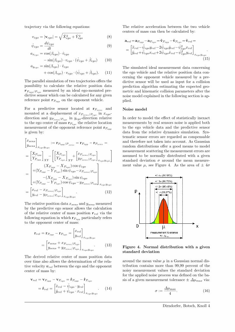
In order to model the effect of statistically inexactmeasurements by real sensors noise is applied bothto the ego vehicle data and the predictive sensordata from the relative dynamics simulation. Sys-tematic sensor errors are regarded as compensableand therefore not taken into account. As Gaussianrandom distributions offer a good means to modelmeasurement scattering the measurement errors areassumed to be normally distributed with a givenstandard deviation σ around the mean measure-ment value µ, see Figure 4. As the area of ± 4σ

Figure 4. Normal distribution with a givenstandard deviation

around the mean value µ in a Gaussian normal dis-tribution contains more than 99,99 percent of thenoisy measurement values the standard deviationfor the applied noise process was defined on the ba-sis of a given measurement tolerance ± ∆µmax via:

σ :=∆µmax

4. (16)


The following equations show the noisy measure-ments for the ideal ego state variables velocity vego,yaw rate ψego and the accelerations axego and ayego :

vnoisyego = vego + ηvego(0, σvego

) (17)

anoisyxego= axego

+ ηaxego(0, σaxego

) (18)

anoisyyego= ayego

+ ηayego(0, σayego

) (19)

ψnoisyego = ψego + ηψego(0, σψego

), (20)

where η(µ, σ) denotes a Gaussian random variablewith mean µ and variance σ2.

The noisy measurements for the ideal predictivesensor data xrel and yrel as well as for the ideallydetected opponent length Wsens are given by:

xnoisysens = xsens + ηxsens(0, σxsens

) (21)

ynoisysens = ysens + ηysens(0, σysens

) (22)

Wnoisysens = Wsens + ηWsens(0, σWsens). (23)

Figure 5 shows an example for ideal and discretenoisy measurement data over time.

Figure 5. Ideal and discrete noisy measure-ment data over time

For the further analysis steps the standard devia-tion of the noisy ego measurements was regardedas constant over time (assumed values for σ seeTable 1).

Table 1.Assumed standard deviations

for ego sensor noise

sensor σvego 0.075 m/saxego

0.050 m/s2ayego

0.050 m/s2ψego 0.005 rad/s

For the predictive sensor measurements (xsens,ysens and Wsens) a more complex model was ap-plied. The standard deviation σ of the applied mea-surement noise was modeled as distance dependentvia the following linear equation because the maxi-mum resolution of the sensor element limits the de-tection accuracy in a decreasing manner along themeasurement distance:

σ(d) = σ0 · (1 + cd · d). (24)

The measurement distance d was calculated on thebasis of the ideal sensor values xsens and ysens:

d =√x2sens + y2

sens. (25)

The assumed basic standard deviations σ0 for thepredictive sensor are shown in Table 2.

Table 2.Assumed basic standard deviations

for predictive sensor noise

sensor value σxsens 0.125 mysens 0.0625 mWsens 0.075 m

As mentioned in the introduction four predictivesensor variants are used for the Monte Carlo analy-sis in this paper. The variants differ in terms of σ0

and cd as depicted in Table 3.

Table 3.Analyzed predictive sensor variants

sensor variant σ0 cd1 σ 0.05 1/m2 σ 0.10 1/m3 2 · σ 0.05 1/m4 2 · σ 0.10 1/m

The distance dependent standard deviation scalingfactor is illustrated in Figure 6.

COLLISION PREDICTION ALGORITHM

Tracking Model

In order to estimate the position and the velocityof an object—as in common predictive sensors—thediscrete state-space formulation

x[k] = f(x[k − 1],h[k],u[k]) (26)y[k] = h(x[k],w[k]) (27)

is used, with x[k] being the state vector at the timeinstance indexed by k, h the system noise, u the


Figure 6. Distance dependent standard de-viation scaling of the measurement noise

control vector, y the measurement vector, w themeasurement noise, and f and h denote the map-pings describing the dynamic model and the sensormodel. In order to use the well-known notation [8]from (27)—unlike in the rest of the paper—a posi-tion vector [x, y]T is notated as r = [rx, ry]T in thissection. The coordinate system used in the follow-ing is a right-hand coordinate system that has itsorigin in the center of gravity of the ego car and thex-axis points to the front. Since the ego car is mov-ing over ground also the location of the origin of thecoordinate system is fixed only for one sample timeT and then it is updated. Figure 7 visualizes themovement of the ego car and an object between twotime stamps. The coordinate system at time t0−T ,

EGO

S

S′

O x

y

P Pold

t0

t0

t0 − T

t0 − T

x′

y′

yego

O′

Object

Figure 7. Movement of ego car and objectin a sample interval T

having the index k−1, is denoted with S, its originwith O and the coordinate system at time instancet0 with S′ and its origin with O′. During the timeT the coordinate system rotates with the yaw angleyego and the object moves from the point Pold tothe point P . In the following the time instance t0has the index k. Since the sensor type that is inthe focus of this paper measures only positions butadditionally also the velocities of the objects in theenvironment of the car are important, the followingstate vector will be used

x[k] =[rO

′Px,S′ [k], rO

′Py,S′ [k], vOPx,S′ [k], vOPy,S′ [k]

]T, (28)

where rO′P

x,S′ [k] is the relative distance in x-directionbetween the object and the ego car at time in-stance t0 expressed in the coordinate system S′,rO

′Py,S′ [k] the relative distance in y-direction, vOPx,S′ [k]

and vOPx,S′ [k] the components of the velocity vectorover ground but rotated in the coordinate systemS′. The advantages of implementing the trackingusing the velocity over ground instead of the rela-tive velocity are described in [9].

To find a suitable model for the mapping h in thedynamic equation (26) firstly the position and thenthe velocity of ego car and object must be ex-pressed in S′ based on the values in the coordinatesystem S.

The position [rOO′

x,S [k], rOO′

y,S [k]]T of the ego car at t0expressed in the cooridinate system S is

rOO′

x,S [k] = vOx,S [k − 1]T + haOx,S

T 2

2(29)

rOO′

y,S [k] = vOy,S [k − 1]T + haOy,S

T 2

2, (30)

with vOx,S [k − 1] and vOy,S [k − 1] being the vectorcomponents of the velocity over ground rotated inthe coordinate system S, and haO

x,Sand haO

y,Srep-

resenting noise terms which take into account thatduring an time interval T the acceleration of thecar is neglected.

The position [rOPx,S [k], rOPy,S [k]]T of the object at timeinstance t0 expressed in the coordinate system S is

rOPx,S [k] = rOPoldx,S [k − 1]+vOPold

x,S [k − 1]T+ha

OPoldx,S

T 2

2(31)

rOPy,S [k] = rOPoldy,S [k − 1]+vOPold

y,S [k − 1]T+ha

OPoldy,S

T 2

2,

(32)

where [rOPoldx,S [k−1], rOPold

y,S [k−1]]T is the position ofthe object at time t0−T expressed in S, [vOPold

x,S [k−1], vOPold

y,S [k − 1]]T the components of the object’svelocity vector over ground at time t0−T expressedin S, and h

aOPoldx,S

and ha

OPoldy,S

noise terms taking into

account that the acceleration of the object duringa sample interval T is neglected.

With equations (29), (30), (31), and (32) the rela-tive position [rO

′Px,S [k], rO

′Py,S [k]]T between ego car and

object at time instance t0 expressed in S can becomputed as

rO′P

x,S [k] = rOPx,S [k]− rOO′

x,S [k]

= rOPoldx,S [k − 1] + vOPold

x,S [k − 1]T + ha

OPoldx,S

T 2

2

− vOx,S [k − 1]T − haOx,S

T 2

2(33)


rO′P

y,S [k] = rOPy,S [k]− rOO′

y,S [k]

= rOPoldy,S [k − 1]+vOPold

y,S [k − 1]T+ha

OPoldy,S

T 2

2

− vOy,S [k − 1]T − haOy,S

T 2

2. (34)

To express the relative distances rO′P

x,S′ [k] and rO′P

y,S′ [k]in the state vector x[k] a transformation to S′ is nec-essary, i. e., a rotation with the yaw angle yego[k]:

rO′P

x,S′ [k]=cos(yego[k])rO′P

x,S [k]+sin(yego[k])rO′P

y,S [k](35)

rO′P

y,S′ [k]=cos(yego[k])rO′P

y,S [k]−sin(yego[k])rO′P

x,S [k].(36)

The velocity of the object over ground but rotatedinto the coordinate system S is

vOPx,S [k] = vOPoldx,S [k − 1] + h

aOPoldx,S

T (37)

vOPy,S [k] = vOPoldy,S [k − 1] + h

aOPoldy,S

T. (38)

In order to express the velocity of the object overground at time instance t0 in S′ a rotation withyego[k] must be performed

vOPx,S′ [k]=cos(yego[k])vOPx,S [k]+sin(yego[k])vOPy,S [k](39)

vOPy,S′ [k]=cos(yego[k])vOPy,S [k]−sin(yego[k])vOPx,S [k].(40)

All relations required to express the mapping h in(26) are now given by (33), (34), (35), (36), (37),(38), (39) and (40). Since only the yaw rate is mea-surable in cars, the yaw rate is approximated byyego[k] = yego[k] · T . Also it is assumed that thesampling interval T is small so that the noise termshaO

x,Sand haO

y,Scorresponding the the ego car can be

neglected in (33) and (34). The following vectorsand matrices are introduced to find an expressionfor h that can be used in a Kalman filter

R[k] =[

cos(yego[k]T ) sin(yego[k]T )−sin(yego[k]T ) cos(yego[k]T )

],

R[k] =[

R[k] 02×2

02×2 R[k]

], F =

1 0 T 00 1 0 T0 0 1 00 0 0 1

,

G=

T 2/2 0

0 T 2/2T 00 T

, x[k−1]=

rO

′Poldx,S′ [k − 1]

rO′Pold

y,S′ [k − 1]vOPoldx,S′ [k − 1]

vOPoldy,S′ [k − 1]

h[k] =

[h

aOPoldx,S

ha

OPoldy,S

], u[k] =

−vOx,S [k − 1]T

000

.The second component in u[k] is zero since vOy,S [k−1] = 0. Now the dynamic equation (26) can bewritten as

x[k] = F [k]x[k − 1] + u[k] + G[k]h[k], (41)

with

F [k]=R[k]F , u[k]=R[k]u[k], and G[k]=R[k]G.(42)

Since the sensor type that is considered in this pa-per measures only the relative position the mea-

surement vector is y[k] =[rO

′Px,S′ [k], rO

′Py,S′ [k]

]Tand

(27) can be expressed as

y[k]=[

1 0 0 00 1 0 0

]x[k]+w[k]=Hx[k]+w[k].

(43)

With the dynamic equation (41) and the measure-ment equation (43) it is straightforward to applya Kalman filter [8] in order to estimate the statevector x[k].

Computation of collision parameters

A collision prediction algorithm has to anticipatethe prospective motion of the ego vehicle and sur-rounding objects on the basis of realistic movementassumptions and estimate the expected collision pa-rameters under the given premises. The predic-tion may both depend on kinematic ego state dataand relative object measurement data provided bya predictive sensor mounted on the moving ego ve-hicle. The prediction process is necessary becausea predictive sensor is usually not able to measurethe geometric and kinematic impact conditions inadequate precision right before the collision. Thisresults from limitations in the sensor field of viewas well as the necessary time interval for the objectcreation and the movement tracking algorithms.

For an online estimation of the collision effect in theego vehicle the geometric and kinematic initial con-ditions of the impact have to be described explicitlyby the predicted collision parameters. Thereforethe following parameters defining the relative posi-tion and movement of the ego and opponent bound-ing boxes at the time of collision were selected, seeFigure 8.

The relative geometric and kinematic movementstate of the two vehicle bounding boxes is described


Figure 8. Predicted collision parameters asinitial conditions of the mechanical impact

by the relative reference point position xcoll in xego-direction and ycoll in yego-direction as well as thegeometric angle φgeom between the vehicle longi-tudinal axes (in Figure 8 the slip angles of bothvehicles are chosen negligibly small) in combina-tion with the ego width Wego, the ego length Lego,the opponent width Wopp and the opponent lengthLopp. As a real predictive sensor will mostly notbe able to detect the complete opponent length theparameter Lopp may also refer to the current lengthof the detected part of the opponent vehicle. Theimpact direction is specified by the angle φvrel

be-tween the relative velocity vector and the ego veloc-ity vector as well as the absolute value vrel of therelative velocity vector. Furthermore the expectedtime to collision (TTC) is estimated on the basisof the underlying assumptions. For this study thecollision parameters were calculated on the basisof a no change assumption concerning the currentmovement state of the ego vehicle and the opponentin two dimensions over ground. The assumptionno change extrapolates the actual moving state ofthe ego vehicle and the opponent sensor object onthe basis of a Taylor series for kinematic state vari-ables. The closer the collision comes the better theno change assumption is able to predict values thatfit the real development of the accident scenario.

The ego and object trajectories are calculated onthe basis of the following correlations concerningthe predicted movement state at t0 defined by thevelocity v, the yaw angle ψ and the slip angle βalong the prediction time tpred:

v(tpred) = v(t0) +dv

dt(t0) · tpred

+12· d

2v

dt2(t0) · t2pred + ...

≈ v(t0) +dv

dt(t0) · tpred (44)

ψ(tpred) = ψ(t0) +dψ

dt(t0) · tpred

+12· d

2ψ

dt2(t0) · t2pred + ...

≈ ψ(t0) +dψ

dt(t0) · tpred (45)

β(tpred) = β(t0) +dβ

dt(t0) · tpred

+12· d

2β

dt2(t0) · t2pred + ...

≈ β(t0) +dβ

dt(t0) · tpred. (46)

On the basis of the movement state variable approx-imations at each prediction time step the vehiclevelocity vector v can be calculated by:

v (tpred) =[v(tpred) · cos(ψ(tpred) + β(tpred))v(tpred) · sin(ψ(tpred) + β(tpred))

]xy

.

(47)

The absolute vehicle position r along the predictedtrajectory can then be calculated by integration:

r (tpred) =

tpred∫t0

v(tpred) · dtpred =[x(tpred)y(tpred)

]xy

.

(48)

The absolute acceleration a along the trajectory isgiven by:

a(tpred) =d

dtpredv(tpred) =

=[

v(tpred)v(tpred) · (ψ(tpred) + β(tpred))

]xvyv

=[alon(tpred)alat(tpred)

]xvyv

. (49)

The resulting trajectory on the basis of a givenand numerically extrapolated working point of theego vehicle movement is shown in the Figure 9. Inthis case the ego slip angle βego is assumed to beknown with a diminishing slip rate βego so thatit remains constant during the prediction. Boththe ego vehicle state as well as the opponent ve-hicle movement are predicted on the basis of thedescribed no change trajectory extrapolation, seeFigure 10. Whereas for the ego vehicle the accel-eration, yaw rate and the slip angle are assumedto be known for the opponent vehicle detected bythe predictive sensor only the velocity in xego- andyego-direction is used for the prediction but not itsacceleration, yaw or slip rate. This assumption is


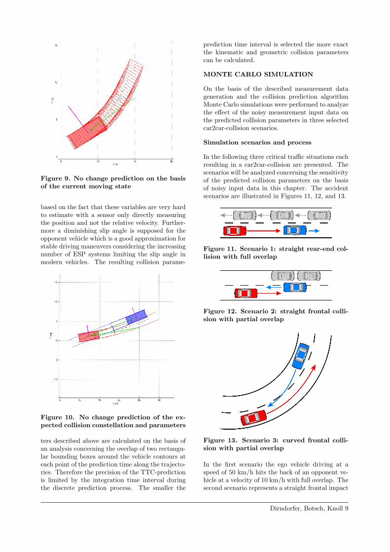
Figure 9. No change prediction on the basisof the current moving state

based on the fact that these variables are very hardto estimate with a sensor only directly measuringthe position and not the relative velocity. Further-more a diminishing slip angle is supposed for theopponent vehicle which is a good approximation forstable driving maneuvers considering the increasingnumber of ESP systems limiting the slip angle inmodern vehicles. The resulting collision parame-

Figure 10. No change prediction of the ex-pected collision constellation and parameters

ters described above are calculated on the basis ofan analysis concerning the overlap of two rectangu-lar bounding boxes around the vehicle contours ateach point of the prediction time along the trajecto-ries. Therefore the precision of the TTC-predictionis limited by the integration time interval duringthe discrete prediction process. The smaller the

prediction time interval is selected the more exactthe kinematic and geometric collision parameterscan be calculated.

MONTE CARLO SIMULATION

On the basis of the described measurement datageneration and the collision prediction algorithmMonte Carlo simulations were performed to analyzethe effect of the noisy measurement input data onthe predicted collision parameters in three selectedcar2car-collision scenarios.

Simulation scenarios and process

In the following three critical traffic situations eachresulting in a car2car-collision are presented. Thescenarios will be analyzed concerning the sensitivityof the predicted collision parameters on the basisof noisy input data in this chapter. The accidentscenarios are illustrated in Figures 11, 12, and 13.

Figure 11. Scenario 1: straight rear-end col-lision with full overlap

Figure 12. Scenario 2: straight frontal colli-sion with partial overlap

Figure 13. Scenario 3: curved frontal colli-sion with partial overlap

In the first scenario the ego vehicle driving at aspeed of 50 km/h hits the back of an opponent ve-hicle at a velocity of 10 km/h with full overlap. Thesecond scenario represents a straight frontal impact


with an overlap of 40 percent within which the egovehicle at a velocity of 50 km/h collides with theopponent vehicle driving at a speed of 40 km/h.In the last scenario the opponent vehicle driving at57.4 km/h leaves its lane on a curved road segmentand collides frontally with the oncoming ego vehiclewith a velocity of 56.2 km/h. For simplicity con-cerning the further analysis steps the selected sce-narios are all stationary concerning velocities, yawand slip rates. Of course dynamic scenarios withsudden break or steering inputs can also be evalu-ated with the proposed method. For the simulationprocess both vehicles are assumed to be equally di-mensioned with a length of 5 m and a width of 2 m.

For the sensitivity analysis of the collision para-meter calculation on the basis of the Monte Carlomethod for each collision scenario 1000 simulationruns were performed with MATLAB/Simulink [10]at a sample time of 1 ms for a sufficiently exact dy-namics simulation. In each scenario Gaussian noisewith the assumed standard deviation (see Chapter“Noise Model”) was added to the ideal measure-ments at a discrete measurement sample time of20 ms modeling the processing cycle for ego andpredictive sensor data. For every scenario two ref-erence time stamps in relation to the actual time ofcollision (TOC) at TOC - 400 ms and TOC - 100 mswere selected. The reference collision parameterswere calculated on the basis of the ideal dynamicsdata. At every reference time step of a scenario thepredicted collision parameters on the basis of thenoisy input values for the collision prediction mod-ule as well as the corresponding reference valueswere logged. The resulting differences between theprediction outputs and the reference values were an-alyzed concerning the statistical mean and standarddeviation as well as the minimum and maximumvalues. The input values for the collision predictionmodule at each time step over all the 1000 simula-tion runs per scenario were all normally distributedwith the given (distance dependent) standard devi-ation around the nominal value and a noise valuelimitation to the ± 4σ interval. The simuation runswere performed with constant ego sensor noise pa-rameters and the four predictive sensor noise vari-ations according to section “Noise model”.

Simulation results

In the following the results of the Monte Carlo sim-ulation process are illustrated. For each of the threesimulated collision scenarios introduced in the lastsection the noisy predictive sensor data as input forthe collision prediction module as well as the re-sulting differences ∆TTC, ∆vrel, ∆φvrel

, ∆φgeom,∆xcoll and ∆ycoll between the prediction outputsand the reference values are presented for two ref-

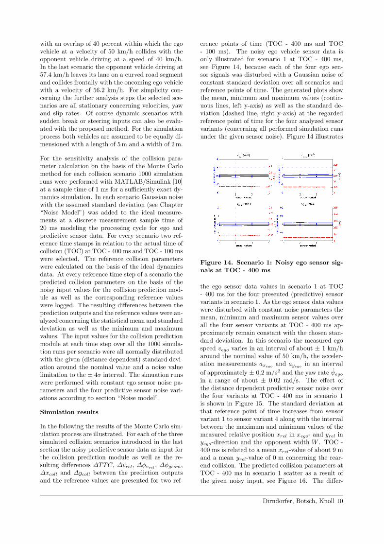
erence points of time (TOC - 400 ms and TOC- 100 ms). The noisy ego vehicle sensor data isonly illustrated for scenario 1 at TOC - 400 ms,see Figure 14, because each of the four ego sen-sor signals was disturbed with a Gaussian noise ofconstant standard deviation over all scenarios andreference points of time. The generated plots showthe mean, minimum and maximum values (contin-uous lines, left y-axis) as well as the standard de-viation (dashed line, right y-axis) at the regardedreference point of time for the four analyzed sensorvariants (concerning all performed simulation runsunder the given sensor noise). Figure 14 illustrates

Figure 14. Scenario 1: Noisy ego sensor sig-nals at TOC - 400 ms

the ego sensor data values in scenario 1 at TOC- 400 ms for the four presented (predictive) sensorvariants in scenario 1. As the ego sensor data valueswere disturbed with constant noise parameters themean, minimum and maximum sensor values overall the four sensor variants at TOC - 400 ms ap-proximately remain constant with the chosen stan-dard deviation. In this scenario the measured egospeed vego varies in an interval of about ± 1 km/haround the nominal value of 50 km/h, the acceler-ation measurements axego

and ayegoin an interval

of approximately ± 0.2 m/s2 and the yaw rate ψegoin a range of about ± 0.02 rad/s. The effect ofthe distance dependent predictive sensor noise overthe four variants at TOC - 400 ms in scenario 1is shown in Figure 15. The standard deviation atthat reference point of time increases from sensorvariant 1 to sensor variant 4 along with the intervalbetween the maximum and minimum values of themeasured relative position xrel in xego- and yrel inyego-direction and the opponent width W . TOC -400 ms is related to a mean xrel-value of about 9 mand a mean yrel-value of 0 m concerning the rear-end collision. The predicted collision parameters atTOC - 400 ms in scenario 1 scatter as a result ofthe given noisy input, see Figure 16. The differ-


Figure 15. Scenario 1: Noisy predictive sen-sor signals at TOC - 400 ms

Figure 16. Scenario 1: Predicted collisionparameters at TOC - 400 ms

ence between the predicted and the reference valuevaries between a resulting minimum and maximumvalue for each collision parameter. In this case forevery parameter the difference increases along withthe sensor variant. The predicted TTC varies inan interval smaller than ± 100 ms around the ref-erence value for all the considered sensor variants.The mean ∆TTC-value is not exactly 0 ms becauseof the prediction tolerance due to the discrete pre-diction time interval of 10 ms. The relative ve-locity vrel was predicted with a tolerance betterthan ± 5 km/h decreasing from sensor variant 4down to 1. The predicted geometric collision an-gle φgeom is more diffuse than the relative velocityangle φvrel

. Both parameters were estimated withan accuracy better than ± 14 concerning the ref-erence in all sensor variants. The predicted relativecollision location parameter xcoll only varies in aquite small range of about ± 0.2 m. The predictedlateral collision opponent location ycoll scatters ina wider range of up to approximately ± 0.5 m. Atthe examined point of time the accuracy of the pre-


diction decreases from sensor variant 1 to sensorvariant 4 for all collision parameters. At TOC -100 ms in scenario 1 the predicted TTC variesin a decreased interval of about ± 50 ms aroundthe reference value in all sensor variants based onsmaller predictive input parameter variations, seeFigures 17 and 18. The relative velocity vrel ispredicted with an accuracy of approximately ± 4km/h. As seen above the predicted relative veloc-ity angle φvrel

again doesn’t scatter as much as thegeometric collision angle φgeom. Both parametersremain in an interval smaller than about ± 12 overall sensor variants. The relative collision location ispredicted relatively exact in xego-direction (± 0.20m) and doesn’t exceed an interval of ± 0.25 m inyego-direction. As a result of the decreasing predic-tive sensor input noise at TOC - 100 ms comparedto TOC - 400 ms the collision parameters are esti-mated with a better (or at least identical) accuracyfor all sensor variants.





In scenario 2 at TOC - 400 ms, see Figures 19and 20, the predicted TTC varies in a maximuminterval of about ± 60 ms around the referencevalue in an increasing manner along the predictivesensor variant due to the growing sensor noise atthat point of time. The relative velocity vrel is pre-dicted with a minimum accuracy of approximately± 6 km/h. Again the predicted relative velocityangle φvrel

doesn’t vary as much as the geometriccollision angle φgeom. Both parameters remain inan interval smaller than about ± 5 over all sensorvariants. The relative collision location xcoll is pre-dicted in a range of about ± 0.3 m in xego-directionand doesn’t exceed an interval of ± 0.6 m in yego-direction. At TOC - 100 ms in scenario 2 theTTC variation interval decreases to approximately± 20 ms due to the significantly smaller predictivesensor noise, see Figures 21 and 22. Whereas theprediction scatter intervals for the relative velocityvrel, the geometric angle φgeom, the relative veloc-ity angle φvrel

and the xcoll-location parameter donot change significantly compared to the values at



TOC - 400 ms, the prediction of the ycoll-parametergets significantly better. This results both from theless scattering yrel-values at TOC - 100 ms as wellas the decreasing effect of errors in the movementprediction direction with a decreasing distance.






In collision scenario 3 the predictive measurementscattering monotonically increases over all sensorvariants at each reference point of time and de-creases from TOC - 400 ms to TOC - 100 ms, seeFigures 23 to 26. As both vehicle trajectories are

curved and the yaw and slip rate of the opponentvehicle are not estimated in the collision predictionmodule the no change prediction assumes a straightopponent trajectory that doesn’t take into accountthe lateral opponent vehicle movement. This re-sults in a visible difference of the mean predictionvalues for the relative velocity vrel and the colli-sion angles φvrel

and φgeom as well as the lateralcollision location ycoll in yego-direction from thereference values. The depicted difference betweenthe mean values for the predicted collision anglesand the ycoll-location parameter gets smaller fromTOC - 400 ms to TOC - 100 ms because the effectof the inexact movement assumption decreases witha smaller distance. In this case the inexact col-lision parameter prediction is not only influencedby the measurement value scattering but also bythe inexact movement assumption in the opponenttrajectory generation. The measurement scatter-ing effects on the predicted collision parameters aresimilar to those observed in scenarios 1 and 2.

CONCLUSIONS

The optimization of passive safety applications bythe use of predictive sensor data requires a suf-ficiently exact prediction of collision parameterscharacterizing the type and severity of a collision.Ego vehicle state sensors as well as predictive sen-sors only measure with a given tolerance and res-olution so that predicted geometric and kinematiccollision parameters always scatter depending onthe characteristics of the applied sensors as well asthe sensor signal processing steps. In this papera method for the model-based evaluation of sen-sor noise effects on the predicted collision parame-ters along the whole signal processing chain witha predictive sensor able to measure distances butnot velocities was presented. On the basis of thedeveloped method a study on the effects of mea-surement scattering concerning the predicted colli-sion parameters was accomplished. Therefore fixednoise parameters for the ego vehicle sensors and twodifferent basic noise levels for the predictive sensorcombined with two noise dependencies along themeasurement distance were assumed. Their effectson the collision parameter prediction were analyzedin three selected collision scenarios. Whereas in thestraight collision scenarios the mean values of thepredicted collision parameters based on noisy inputdata fitted the reference values very accurately incurved scenarios the collision prediction algorithmassuming a straight trajectory for the opponent ve-hicle (as opponent yaw rates are very hard to es-timate) resulted in a time-dependent mean valuein the geometric parameter prediction. Depend-ing on the sensor noise parameters the geometric


collision parameters in all analyzed scenarios scat-tered in a specific range representing the accuracyof the prediction under the given premises. For thethree analyzed scenarios under the made assump-tions the TTC prediction scattering at TOC - 400ms and TOC - 100 ms didn’t exceed a range of ±100 ms around the reference value, the relative ve-locity angle prediction was always in an interval of± 9 and the predicted geometric angle varied in amaximum interval of ± 18 . The relative referencepoint position in longitudinal ego vehicle body di-rection scattered in a range of ± 0.30 m at mostand the relative reference point position in lateralego body direction differed in a maximum range of± 0.60 m (at TOC - 400 ms) respectively ± 0.25 m(at TOC - 100 ms) in straight scenarios and in arange from -0.10 m to -1.30 m (at TOC - 400 ms)respectively -0.50 m to 0.10 m (at TOC - 100 ms) inthe curved scenario. The results show the challengeof collision predictions in the case of small vehicleoverlaps and in curved scenarios. For the reliabledetection and prediction of the collision parametersin these scenarios the sensor noise parameters haveto be kept low in combination with an adequate dy-namic object tracking with ego-compensation evenin areas close to the ego vehicle. The effect of dy-namic scenarios with sudden steering or brake in-puts concerning the parameter prediction was notyet analyzed and has to be observed in future stud-ies.

REFERENCES

[1] Eichberger, A., Wallner, D., Hirschberg, W.2009. “A situation based method to adapt thevehicle restraint system in frontal crashes tothe accident scenario.” Proceedings of the 21stESV Conference; International Conference onthe Enhanced Safety of Vehicles, 2009.

[2] Moritz, R. 2000. “Pre-crash sensing - func-tional evolution based on short range radarsensor platform.” SAE Technical Paper Series,00IBECD-11, 2000.

[3] Skutek, M., Linzmeier, D.T., Appenrodt, N.,Wanielik, G. 2005. “A precrash system basedon sensor data fusion of laser scanner and shortrange radars.” IEEE 8th International Confer-ence on Information Fusion, 2005.

[4] Gietelink, O., Ploeg, J., De Schutter, B.,Verhaegen, M. 2006. “Development of ad-vanced driver assistance systems with vehiclehardware-in-the-loop simulations.” Technicalreport, Delft University of Technology, 2006.

[5] Pudenz, K. 2010. “Der Audi A7 Sportback:Sicherheitssysteme.” ATZonline, July 2010.

[6] Karrenberg, S. 2008. “Zur Erkennung un-vermeidbarer Kollisionen von Kraftfahrzeugenmit Hilfe von Stellvertretertrajektorien.” Tech-nical report, Technische Universitat Carolo-Wilhelmina zu Braunschweig, 2008.

[7] Mitschke, M., Wallentowitz, H. 2004. “Dy-namik der Kraftfahrzeuge.” Springer, 2004.

[8] Bar-Shalom, Y., Li, X. R., Kirubarajan, T.2001. “Estimation with Applications to Track-ing and Navigation.” John Wiley & Sons, July2001.

[9] Altendorfer, R. 2009. “Observable dynamicsand coordinate systems for automotive targettracking.” IEEE Intelligent Vehicles Sympo-sium, 2009.

[10] MATLAB 2009b, Copyright c© 1984-2009 TheMathWorks Inc.


model-based analysis of sensor-noise in predictive passive ... · model-based analysis of...

Documents