model development and empirical tests based on swedish
TRANSCRIPT
THE ASSOCIATION BETWEEN
ACCOUNTING INFORMATION AND STOCK PRICES
Model developmentand
empirical tests based on Swedish data
Mikael Runsten
AKADEMISK AVHANDLING
for avlaggande av ekonomie doktorsexamenvid Handelshogskolan i Stockholmframlagges till offentlig granskning
fredagen den 18 september 1998klockan 13.15 i sal 550
Handelshogskolan, Sveavagen 65


The Association betweenAccounting Information and Stock Prices
Model developmentand
empirical tests based on Swedish data

(;i~ STOCKHOLM SCHOOL OF ECONOMICS~~,,:tfll EFI, THE ECONOMIC RESEARCH INSTITUTE
EFI MissionEFI, the Economic Research Institute at the Stockholm School of Economics, is a scientificinstitution which works independently of economic, political and sectional interests. Itconducts theoretical and empirical research in management and economic sciences,including selected related disciplines. The Institute encourages and assists in thepublication and distribution of its research findings and is also involved in the doctoraleducation at the Stockholm School ofEconomics.EFI selects its projects based on the need for theoretical or practical development of aresearch domain, on methodological interests, and on the generality of a problem.
Research OrganizationThe research activities are organized in twenty Research Centers within eight Research Areas.Center Directors are professors at the Stockholm School of Economic.
ORGANIZATION AND MANAGEMENTManagement and Organisation Theory (A)Public Management (F)Information Management (I)Man and Organisation (PMO)Industrial Production (T)
MARKETINGInformation and Communications (CIC)Risk Research (CFR)Marketing, Distribution and Industrial Dynamics (D)Distribution Research (FDR)Economic Psychology (P)
ACCOUNTING, CONTROL AND CORPORATE FINANCEAccounting and Managerial Finance (B)Managerial Economics (C)
FINANCEFinance (FI)
ECONOMICSHealth Economics (ClIE)International Economics and Geography (lEG)Economics (S)
ECONOMICS STATISTICSEconomic Statistics (ES)
LAWLaw (RV)
OTHERSEthics and Economics (CEE)Policy Sciences (PSC)
Prof. Sven-Erik SjostrandProf. Nils BrunssonProf. Mats LundebergProf. Jan LowstedtProf. Christer Karlsson
Adj Prof. BertH ThorngrenProf. Lennart SjobergProf. Lars-Gunnar MattssonActing Prof. Richard WahlundProf. Lennart Sjoberg
Prof. Lars OstmanProf. Peter Jennergren
Prof. Clas Bergstrom
Prof. Bengt JonssonProf. Mats LundahlProf. Lars Bergman
Prof. Anders Westlund
Prof. BertH Wiman
Adj Prof. Hans de GeerAdj Prof. Brita Schwarz
AdministrationChairman ofthe Board: Prof. Sven-Erik Sjostrand. Director: Ekon Dr Rune Castenas
A dressEFI, Box 6501, S-113 83 Stockholm, Sweden • Internet: www.hhs.se/eft.!Telephone: +46(0)8-736 90 00 • Fax: +46(0)8-31 62 70 • E-mail [email protected]

THE ASSOCIATION BETWEEN
ACCOUNTING INFORMATION AND STOCK PRICES
Model developmentand
empirical tests based on Swedish data
Mikael Runsten
t4\ STOCKHOLM SCHOOL OF ECONOMICS"\\J;' EFI, THE ECONOMIC RESEARCH INSTITUTE

l1'l\ A Dissertation for the,!'!Y(1)i!'11 Doctor's Degree in Philosophy'~!I Stockholm School of Economics, 1998
© EFI and the authorISBN 91-7258-489-0
Key Words:AccountingConservativeEarningsMeasurementReturn on equityStock pricesSwedenValuation
Distributed by:The Economic Research Institute at the Stockholm School of Economics,Box 6501,113 83 Stockholm, Sweden
Printed by Elanders Gotab, Stockholm 1998
Preface
This report is a result of a research project carried out at the department ofAccounting and Managerial Finance at the Economic Research Institute(EFI) at the Stockholm School ofEconomics.
This volume is submitted as a doctor's thesis at the Stockholm School ofEconomics.
The Institute is grateful for the financial support provided by RuneHoglunds minnesfond, Jan Wallenders stiftelse, Svenska Handelsbanken,Institutet far faretagsledning-IFL, and Price Waterhouse,.
As usual at the Economic Research Institute, the author has been entirelyfree to conduct and present his research in his own ways as an expression ofhis own ideas.
Stockholm in July 1998
Rune CastenasDirectorThe Economic Research Institute
Lars OstmanProfessorHead of Department forAccounting and~anagerialFinance


ACKNOWLEDGMENTSMy career as a doctoral student started many years ago. I spent a number ofyears thinking that my thesis would deal with incentive schemes, but waseventually only happy with the title-"Performance beyond Survival". Thenmy attention switched to the topic of this manuscript in the late 1980s. Noone, certainly not myself, could foresee 110w long this research projectwould take. I am greatly indebted to many people for sharing their insightswith me and for making the process such a happy journey.
First of all, I would like to thank Professor Kenth Skogsvik, my thesiscommittee chairman and Professor Lars Ostman, my former chairman. BothLars and Kenth have contributed enormously in different ways over theyears. Besides offering plenty of research advice, they have gently applied amixture of carrots, sticks and other stimuli. But most importantly they haveprovided an exceptional amount of trust and patience. Thank you.
I am also very grateful to the third member of my thesis committee, Professor Peter Jennergren, who above all has helped clarify my economic modeling.
Professor emeritus Sven-Erik Johansson has, over the years, offered numerous stimulating ideas regarding everything from details of accounting to theart of the proper use of a golf tee. Sven-Erik has also generously offered anumber of invaluable suggestions concerning the final draft of this thesis.
In the early phase of my research, a 'traveling research group' consisting ofmy colleagues Kenth Skogsvik (who later became my thesis committeechairman), Peter Kahari, Magnus Bild and myself, spent numerous hoursdiscussing our research projects aboard various trains destined formetropolises such as Andalsnas and Berlin. Peter and Magnus also deservementioning. Peter has been close friend and a trusty gillie. I particularlyadmire Peter's talent for raising basic but difficult research questions. Peterhas also been an important source of inspiration in the art of teaching.

Accounting Information and Stock Prices
Magnus has been a 'true mate'; he has offered numerous suggestionsregarding my work and, towards the very end, he very generously took onsome of my other responsibilities, to allow me to dedicate my self tofinishing this manuscript. Magnus is also very resourceful in theconceptualization and implementation of practical jokes, which hasprovided many enjoyable mon1ents.
Many thanks are due to several other colleagues at the Stockholm School ofEcol10mics, wl10 have provided valuable comments and feedback on different drafts; Professor Lars Samuelsson, Associate Professor Walter Schusterand numerous fellow doctoral students, including Niklas Hellman, HansHallefors, Anja Lagerstrom and Tomas Hjelstrom are hereby gratefully acknowledged. Leif Eriksson, teacher and subsequently co-teacher on manymanagement courses at the Swedish Institute of Management (IFL), has provided perceptive con1ments on my research, and enjoyable company, but hasforemost been an important role model for me as a teacher. AssociateProfessor Per-Olov Edlund has been a very helpful and knowledgeablesource of insights on statistical matters.
To the remaining group of people that for me constitute 'B-sektionen'-Siv,Karin, Vanja, Peter, Ulf, Jorgen, Kerstin, Matti, Per, Hans, Claes, Ingrid,Sten, Mats, Goran, Helena, Lars, Birgit, Christer, Stina, Bertil, Gunnar, Elvi,Catharina, Goran, Steen, Ulrika, Ulrika, Alee, Katerina-thank you forsmiling back.
I very much appreciate valuable suggestions I have received on differentoccasions from Professors Jan1es Orllson, Ray Ball and Stephen Zeff.
The empirical part of this research is based on data compiled by Findata.Findata has generously allowed me to access their database, without whichthis research could not have been conducted. Furthermore, I would like tothank Erik Eklund, one of the co-founders of Findata, who has always beenwilling to discuss detailed data n1atters.
Maria De Liseo proofread this manuscript and I am very grateful for hermany suggestions which no doubt have made my English more readable.
11

Acknowledgements
Dr. Rune Castenas at the Economic Research Institute (EFI) of the Stockholm School of Economics has been very helpful in finding financial support for this project. In this context, I am especially grateful to RuneHoglunds stiftelse, Svenska Handelsbanken, Jan Wallanders stiftelse, theSwedish Institute of Management (IFL), and Price Waterhouse.
I was very fortunate to spend a year at the University of California,Berkeley, and at Stanford University. Both can1puses offered a very stimulating academic environment which contributed immensely to my development. My year in California is in many respects very special to me. I wasvery lucky to get to know my dear friend Udo Zander-the source of manywitty discussions and good entertainment. Many thanks to all the artists ofCircus Alvarado, and particularly Udo, Greg, Dechen and Rick. I am mostgrateful to the Fulbright Commision, C. Silvens stiftelse and the ChilesFoundation for making my stay in the US possible. The personal supportoffered by Earle Chiles and his generous hospitality towards my wife andmyself during our visit to Portland is gratefully remembered.
In my childhood, while working on different construction projects with myfather, I learned that any creative endeavor require two essential ingredients:i) an element of luck which is essential and must be allowed for, ii) time tosit back and enjoy any small achievement. In other words, improvise, seethe opportunities and enjoy the process. Thank you for these lessons which Ihave applied liberally over the years.
Finally, to my wife Eola-thank you for being who you are, and thank youfor letting me be who I am.
Despite the contributions made by all these people, deficiencies in thisthesis still remain. They are entirely my own.
Mikael Runsten
StockholmJuly 1998
iii

CONTENTS
PART I THEORETICAL FRAMEWORK AND RESEARCH
DESIGN
1 INTRODUCTION AND BACKGROUND .....•••.••.••.•.•••.•••••••••••••••..•.•••••.••••.•••••••3
1.1 ECONOMIC, MARKET AND ACCOUNTING VALUE 3
1.2 PREVIOUS RESEARCH 101.3 PURPOSE 171.4 DISCUSSION OF THE PURPOSE, LIMITATIONS AND ASSUMPTIONS 17
1.5 DISTINCTIVE FEATURES AND EXPECTED CONTRIBUTIONS 18
1.6 STRUCTURE OF THIS DOCUMENT 20
2 A VALUATION FRAMEWORK.••••••••..•••.••••••••••••••••.•••••••••••••••••••••••••••••.••••••••• 21
2.1 A VALUATION APPROACH 222.2 THE VALUATION MODEL WITH DISAPPEARING ABNORMAL PROFIT 25
2.3 THE VALUATION MODEL GIVEN A PRUDENT ACCOUNTING REGIME 312.4 A NUMERICAL EXAMPLE 38
2.5 THE VALUATION MODEL IN EMPIRICAL TESTS 412.5.1 Regression specifications for value level studies 44
2.5.2 Model and regression specifications for value change studies 462.5.3 Analysis of the different elements of the regression models 51
3 RESEARCH DESIGN CONSIDERATIONS 57
3.1 FIRM CHARACTERISTICS 57
3.1.1 Expected accounting measurement bias (in capital terms) 583.1.1.1 Sources of the measurement bias for different balance sheet items 59
3.1.1.2 Principal estimation procedure of the measurement bias 68
3.1.1.3 Calculation of the most significant measurement biases 71
3.1.1.4 The measurement bias as calculated by Fruhan 84
3.1.2 Expected growth persistence factor (GPF) 88
v

3.1.3 Expected validity of historical ROE 88
3.1.4 Summarized description of frrm characteristics 89
3.2 CHANGES IN THE ECONOMIC CLIMATE 91
3.3 ACCOUNTING CHANGES 92
3.3.1 Accounting changes in Sweden 1965 - 1995 94
3.3.1.1 Mandatory consolidated statements 99
3.3.1.2 Open disclosure of inventory reserves and depreciation according to plan. 99
3.3.1.3 Consolidation method and accounting for goodwill 103
3.3.1.4 Accounting for associated companies 104
PART II SAMPLE SELECTION, MEASUREMENT AND
ESTIMATION OF MODEL PARAMETERS
4 SAMPLE SELECTION AND MEASUREMENT OF BASIC MODEL
PARAMETERS ........................................................•..••••••.•......•......••••••..•....•••.••. 109
4.1 SAMPLE SELECTION 109
4.2 THE MEASUREMENT OF CURRENT ROE, THE ESTIMATION OF REQUIRED RETURN
AND THE PREDICTION OF FUTURE ROE 113
4.2.1 Measurement of earnings, shareholders' equity and ROE 113
4.2.1.1 Chosen definition of earnings 114
4.2.1.2 Chosen definition of equity 114
4.2.1.3 Operationalization of the chosen definitions 115
4.2.1.4 Measurement of the annual tax rate 116
4.2.1.5 Description of the data 117
4.2.2 Required rate of return or the cost of equity capita1. 122
4.2.3 Prediction of ROE for the next period-eonceptually 128
4.2.3.1 Earnings forecasts 129
4.2.3.1.1 Univariate mechanical approaches 129
4.2.3.1.2 Multivariate mechanical approaches 130
4.2.3.1.3 Non-mechanical approaches 131
4.2.3.1.4 Conclusions regarding the earnings process 132
4.2.3.2 Return on equity forecasts 132
4.2.3.3 Choice of forecasting approach 134
VI

5 OPERATIONALIZATIONS ...••••••••••••••••••...•••••.•••.•••••••••••.•.••••••••••••.•.••••••..•••.• 140
5.1 ESTIMATION AND CLASSIFICATION OF FIRM CHARACTERISTICS 140
5.1.1 The permanent accounting measurement bias 1405.1.1.1 Marginal PMB related to tangible assets 142
5.1.1.2 Marginal PMB related to intangible assets 146
5.1.1.3 Marginal PMB related to deferred taxes 148
5.1.1.4 Summarized estimated PMBs 149
5.1.2 The hurdle rate (g) increase from the PMB 152
5.1.3 Classification in different GPF-level categories 154
5.1.4 Classification of validity ofhistorical ROE 155
5.2 MEASUREMENT OF CHANGES IN THE ECONOMIC CLIMATE 158
5.2.1 Inflation rate pattern 1585.2.2 Changes in the business climate 161
5.3 DESCRIPTION OF ACCOUNTING CHANGE 1645.3.1 Open disclosure of value and depreciation according to plan 1645.3.2 Group consolidation methods-accounting for acquisitions and treatment
of goodwill 1675.3.3 Accounting for associated companies 171
6 REGRESSION VARIABLES .......•...•..•..••.•..••••.•••.••••••.••.••••••••...••••••••.••••••••••.•• 174
6.1 CALCULATION OF THE MAIN VARIABLES FOR THE SPECIFIED REGRESSION MODELS1746.1.1 Market-to-book value premiums 174
6.1.2 Prediction of ROE for the next period-in practice 1776.1.3 Expected residual return 1826.1.4 Calculation of the dependent and independent variables for the change
specifications 1846.1.4.1 The change in market value 184
6.1.4.2 The change in book value 185
6.1.4.3 The change in expected residual income 187
6.1.4.4 The change in book value tinles the PMB 188
VII

PART III EMPIRICAL RESULTS
7 EMPIRICAL RESULTS: THE LEVEL APPROACH•••••••••••••..•••.••.•..•••••...•• 193
7.1 REGRESSIONMODELM.1 194
7.1.1 The full sample 194
7.1.2 Sub-sample regressions controlling for different expected validity of
historical ROE and GPF levels 197
7.2 REGRESSION MODEL M.2 205
7.2.1 The full sample 205
7.2.2 Sub-sample regressions controlling for different expected validity of
historical ROE and GPF levels 208
7.3 REGRESSION RESULTS AND CHANGES IN THE ECONOMIC CLIMATE 217
7.3.1 Business cycle fluctuations 217
7.3.2 Changes in the rate of inflation 224
7.4 REGRESSION RESULTS AND LARGE ACCOUNTING CHANGES 228
7.4.1 Open disclosure of depreciation according to plan 228
7.4.2 Regression results and acquisition activity 233
7.4.2.1 Goodwill treatment method 238
7.4.2.2 The pooling versus the purchase method 241
7.4.3 Accounting for associated companies 245
8 EMPIRICAL RESULTS: THE CHANGE APPROACH.........•..•....•.•.••..•.•••• 247
8.1 REGRESSION MODEL M.3 248
8.2 REGRESSION MODEL M.4 253
8.3 REGRESSION MODEL M.S 258
8.3.1 Stability in association over time 260
8.3.2 Different profit recognition characteristics 265
8.3.3 Regression results for different industries 267
8.3.4 A homogenized sub-sample 269
8.4 REGRESSION RESULTS AND CHANGES IN THE ECONOMIC CLIMATE 270
8.4.1 Business cycle fluctuations 270
8.4.2 Changes in the rate of inflation 272
8.5 REGRESSION RESULTS AND LARGE ACCOUNTING CHANGES 276
8.5.1 Open disclosure of depreciation according to plan 276
viii

8.5.2 Regression results and acquisition activity 278
8.5.2.1 Goodwill treatment method 281
8.5.2.2 The pooling versus the purchase method 282
8.5.3 Accounting for associated companies 283
9 SUMMARY AND CONCLUDING REMARKS.....•...••••••••••••.••••.•••••••••.•••••.•. 284
9.1 RESEARCH PROBLEM AND RESEARCH DESIGN 284
9.2 EMPIRICAL RESULTS 290
9.3 THE VALIDITY OF THE APPLIED RESEARCH DESIGN 295
9.4 CONCLUDING REMARKS 302
APPENDICES
Appendix A Table of PMBs-tangible assets 311
Appendix B Table ofPMBs-intangible assets 312
Appendix C Intangible assets-linear depreciation 314
Appendix D Industry classification 315
Appendix E Check of the industry classification 316
Appendix F Number of quoted fmns 318
Appendix G Swedish earnings measurement practice 320
Appendix H Income statement and balance sheet 323
Appendix I Operationalization of accounting information in terms of Findata
variables 324
Appendix J Median balance sheet items 326
Appendix K Partial PMBs related to M&E and ships 327
Appendix L Partial PMBs related to buildings 328
Appendix M Partial PMBs related to investments in shares 329
Appendix N Partial PMBs related to R&D expenditures 330
Appendix 0 Partial PMBs related to deferred taxes 331
Appendix P Business cycle patterns 332
Appendix QAccounting for acquisitions 333
Appendix R Ordinary least squares-statistical considerations 335
Appendix S M.2 regressions results 342
Appendix T Earnings expectations fronl a business magazine for a small group
of companies 343
Appendix U Accounting for depreciation 348
Appendix V Accounting for associated companies 349
ix

SYMBOLS AND ABBREVIATIONS •.••••••...••••.••••••••••••••••••.••.•••••••••••••••••••••.•.•••350
REFERENCES........•.............•...•.......•.....•........••....•••.••....•.•..••••.....•••••••••••••••••.•••••353
x

Part I
THEORETICAL FRAMEWORK AND
RESEARCH DESIGN
1 Introduction and Background2 A Valuation Framework3 Re.search Design Considerations


1 INTRODUCTION AND BACKGROUND
1.1 Economic, market and accounting valueAccording to economic theory, the value of an asset for its owner is the discounted value of all future cash flows which the owner expects to receive asa consequence of the possession and decisions regarding the asset's use. Thevalue of a finn is assumed to ultimately depend on the monetary success ofthe business. Some fimls have many owners and a share that is traded on astock exchange. Observed stock prices are the result of an interactionbetween many individual investors with different transaction motives,expectations of the future, time horizons and analytical nlethods.l The resultof these individual investors' aggregated actions generate market prices.Observed stock prices can be viewed as an aggregated measure of themarket's valuation of the claim on the firm's future value creation. Thus thestock price is an implicit indicator of the market's expectations of the futuresuccess of the firm.
Accounting can be viewed as a language through which an attempt is madeto measure and describe tIle financial consequences of the actions that aretaken within a financial entity. The accounting procedure generates a number of descriptions of the firm. In the balance sheet the firm's assets andliabilities are identified and valued at a particular point in time. The difference between assets and liabilities is labeled owners' equity. Equity is ameasure of the value that the shareholders have a claim on. In the incomestatement an attenlpt is made to describe the revenues that the activitieshave generated during a period and the expenses that the generation of theserevenues has caused.2 The residual, labeled earnings or net income, is a
Some actors represent their own economy directly, whereas an increasing proportion ofthe actors are en1ployed individuals that invest on behalf of the institutions' ultimateowners.
2 Revenues and expenses can, of course, further be specified at different levels of aggregation.

Accounting Information and Stock Prices
measure of the period's value creation, measured after all the firm's stakeholders, except for the shareholders, have received compensation.3
According to the pricing procedure, value is the result of an almost dailyanonymous trading process where, according to financial theory, the expected performance of a firm is balanced into a price via the investors' return requirements. Information is often assumed to constitute the base forthe creation of expectations of firm prospects, and preferences are manifested into required rates of return. Value from the accounting procedure is,011 the other hand, the result of a measurement procedure that follows specific conventions and rules.
Three value and value creation concepts have been identified. Firstly, thevalue concept derived from discounted future cash flows will be called economic value (V).4 This theoretical value concept will be used as a generalpoint of reference. Secondly, market value (M) and accounting value wereidentified. The term book value of equity (B) will often be used rather thanthe term accounting value. Figure 1.1 illustrates the relationship betweenthese three value concepts. The economic value concept is forward looking(expected future cash flows), while the starting point of traditional costbased accounting is actual cash outlays. The market price observed on thestock market is based on trade between investors.
3
4
Most common accounting regimes postulated today rely extensively on valuationaccording to historical cost. This simplified description of accounting, however, doesnot refer to a particular accounting regime.Classical valuation theory was developed by, among others, Fisher (1906) and Lindahl(1939). See discussion in Johansson and Ostman (1995).
4

Introduction and Background
Value Concepts
L"Expected cash
flows from using theresources"
"Actual cash flowsto get hold of
resources".
Base for traditional
Accounting Value
A
B
"Trade betweeninvestors"
Market Value
..-+
Base for
Economic Value
Time
Figure 1.1 An illustration of three major value concepts relating to theshareholders' claim on a company. Assets minus liabilitiesequals book value of equity (A-L=B). The economic value concept is basically forward looking (expected future cash flows),while the starting point of traditional cost-based accounting isactual cash outlays. The market price observed on the stock market is based on trade between investors.
For each value concept, one can also identify a value change or a returnmeasure. Return can relate to expectations (ex ante) or actual outcomes (expost). In a world of certainty, these measures do, of course, coincide.
Value according to econon1ic theory is intimately connected to a discountfactor (r), which is a measure of a fair expected and required return. Thechange in economic value between two points in time plus the period's nettransactions between the owners and the firm (NT = dividends - new issues)equals 'economic income'. The change in value referring to observed market prices plus the period's net transactions is an ex post return concept. In asimilar way, return can be calculated from accounting descriptions. Thechange in accounting equity plus net transactions with the owners equalsaccounting earnings. Earnings divided by opening equity generates thecommonly used ratio return on equity (ROE).
If the accounting procedure generates 'good' descriptions of the firm'svalue and value creation, a close correspondence between accounting equity(the change in equity) and the stock market value of the firm (the change in
5

Accounting Information and Stock Prices
the stock market's valuation of the firm) can be expected. All three valueconcepts may even be made to coincide, provided a set of strong assumptions. Sufficient conditions include perfect markets, individuals with thesame preferences, the same level of wealth, and access to the same information which is treated in an identical way. In order to ensure that ex postreturn is equal to ex ante return, an assumption of certainty is also required.5
These conditions, 110wever, are not particularly realistic. Rather than separate systems generating identical descriptions, one type of description mayin practice facilitate the functioning of the other. The output of theaccounting procedure may, for example, be used as input in the pricing procedure. Different actors can use accounting information for different purposes; stock investors may, for example, use the information to i) form ideasof the firm's financial status, ii) form expectations of future firm performance, and iii) compare realized performance with expected performance andthus when necessary revise expectations.
The following observations can be made:i) Two of the value expressions (M and B) can easily be observed.ii) Value according to economic theory is not possible to observe, but
is a possible ideal for anyone who produces, establishes laws about,or uses values from the accounting procedure.
iii) The valuation approaches of individual actors (PIE ratios, discounted expected cash flows, etc.) may to varying degrees beinspired by or be consistent with economic theory. The result of theindividual investor's aggregated behavior corresponds to M.
Consider the following simple illustration. In figure 1.2 the market and accounting value of Ericsson, the Swedish telecommunications equipmentmanufacturer, is illustrated over tin1e (from 1966 to 1996). The stockmarket's value of the firm (number of shares outstanding times the latest quotedbuying price) has been measured at the end of each month and the accounting value relates to the end of each year. Given that the stock price ofEricsson at any time is assumed to be a function of how investors expect thefirm to perform, it is easy to realize that these expectations may change atany time due to, for example, the market entry of a new competitor, a press
5 See discussion in chapter 3 and 4 in Beaver (1989).
6

Introduction and Background
release regarding an important breakthrough in research, or news of a largeorder. The value of Ericsson measured according to the current accountingregime is, on the other hand, a function of, for example which revenues maybe recognized and how assets should be valued. Events that change expectations of future performance may take time to work their way into registered accounting performance, given a specific accounting regime, or theperformance may never actually materialize (assuming incorrect expectations).
SEK million
Monthly market value andannual accounting equity of Ericsson
1 000 000 -r-----------------------.
100 000 -I------------------------;~r-----t
10000 -l------------I~:cNlNP..,.'W.....------I
Figure 1.2 The market value (the unbroken line) and accounting equity(dots) ofEricsson during the period 1966 to 1996. Market valuehas been measured at the end of each month and accountingequity at the end of each year. Accounting equity includes 50%of untaxed reserves up until 1988 and 70% from then on. (Notethat a logged value scale simplifies the comparison ofthe relativedistance between the two value measures over the relatively longperiod.)(Data has been compiled/rom Dextel-Findata.)
It can be concluded from the figure that the two descriptions seldom agree.At some points in time, the market's valuation exceeded accounting valueand vice versa. Value change, according to the two descriptions, has oftenbeen contradictory for shorter periods. Both descriptions seem, however, tohave followed the same general trend.
7

Accounting Information and Stock Prices
One reason for this not surprisingly imperfect relationship can be found inthe principles of conventional accounting. The prevailing accounting regimeis guided by a number of fundamental principles and compromises. Anaccounting convention relies on specific principles regarding valuation (forexample; historical costs, current costs or exit prices), matching of costs torevenues within a specific period, recognition of income, and so on. Theguiding principles can, for example, put an emphasis on keeping track ofactual historical transactions or their potential consequences for futuretransactions. Kam (1990) argues that the accounting procedure's way ofcalculating an entity's periodic income is a compromise between whatwould have been possible under two extreme circumstances-the terminalcase and the certainty of future case.
HIn our world of uncertainty, determining income is somewherebetween the strict accrual accounting of the ideal case and thecash receipts and cash payments basis ofthe terminal case. "
HIncome determination for a business firm is not a simple task.The cash flows are not known with certainty, and the time horizon is not ascertainable. Yet, because of legal requirements, necessity and convention, periodic income must be calculated. "
Kam (1990, pp. 192 - 193)
Patell (1989) points out that the existence of many potential users of accounting infomlation may have led to a choice of principles that is not optimal given a specific user's perspective.
HTo the extent that we must focus on a single, bottom-line measure of earnings to meet the demands of all of these constituencies,6 compromises may have been reached in determining themeasurement rules, so that some of the potential usefulness inanyone arena (say equity capital markets) has been knowinglysacrificed when that is necessary to enhance utility in other arenas. "
6 Patell discusses different interest groups in terms of different markets. He refers to themarket for equity capital, debt capital, labor, material and products. He further refers tothe political market when discussing the role measurement plays in taxes, tariffs andduties etc.
8

Introduction and Background
The Swedish accounting convention has been forced to compromise in particular between the information interest of creditors and shareholders. Furthermore, a strong impact on chosen accounting principles is due to the factthat the measurement of tax charges in Sweden has been closely linked toaccounting descriptions. Having to cope with the real difficulties of a combination of genuine uncertainty of the future and long-term projects, theSwedish accounting convention has come to emphasize characteristics suchas objectivity and reliability. This has led to measurement rules characterized by prudence and valuation based on documented transactions.7 Thusthe accounting regime has a deliberate tendency to recognize losses earlyand recognize gains late and to valuing assets low and liabilities high. Thevalue of accounting equity for an arbitrary firm calculated according to theSwedish accounting convention cannot therefore be described as attemptingto be the best possible estimate of 'true value'. Neither can accountingearnings be described as the best possible estimate of the period's financialvalue creation:
tiThe realization convention and the convention ofprudence canoften imply a poor matching ofrevenues and expenses and ofincome and capital in measuring rate ofreturn "
Johansson and Ostman (1995, p. 121)
The role and usefulness of accounting information naturally differs depending on the user and for what purposes the information is used.Hendriksen discusses this nlatter from the point of view of different users:
tiManagers seek information that will help them to predict theeffect of current decisions on future cash flows. Stockholderswho have an effective control of management need informationto be able to judge the relative efficiency ofmanagement. Stockholders, prospective investors, and creditors need informationthat will help them predict the future course of the firm and theprobability of future financial success that will permit repayllzents and cash distributions. While these objectives may lead toa single set ofaccounting principles, different sets ofprinciples
7 Note that most of these observations are not typically Swedish, but are probably asvalid for most industrialized economies.
9

Accounting Information and Stock Prices
may be required to meet the several possible goals of accounting. "
Hendriksen (1982, p.11)
The Financial Accountings Standards Board (FASB) characterizes usefulinformation as follows:
H ••• useful information possesses two primary characteristics:relevance and reliability. Information is relevant if it makes adifference in the decision ofthe user, and it is reliable if it represents what it purports to represent. "
FASB concept statement No.2
With reference to the reliability and relevance concepts, one can argue thatfrom the investor's position, the bottom-line measure of earnings disclosedin an income statement can be analyzed from two perspectives:
i) as a measure of the firm's value creation during the period (earningsin a measuren1ent function);
ii) as an indication (or signal) of the firm's ability to create value(earnings in a signaling function).
1.2 Previous researchMost of the classical accounting research has been related to measurementquestions often from a normative perspective without direct reference tostock prices. However, since the late 1960s, US accounting research haslargely been oriented towards price reactions on accounting signals oftenwithout reference to measurement.
With economic value as the point of reference, a classical measurementissue focuses around how well accounting equity and accounting earningsapproximate firm value and income according to economic theory. Examples of research questions include: Which depreciation pattern bestdescribes the 'true' value change of an asset? What biases or errors are introduced in the measurement procedure when a certain accounting convention is used and, for example, inflation is non-zero? Does current costaccounting better approximate theoretical ideals? [Significant contributions
10

Introduction and Background
include: Fisher (1906), Bonbright (1937), Lindahl (1939), Paton andLittleton (1940), Johansson (1961), Edwards and Bell (1961), Mattessich(1964), and Ijiiri (1967). See also recent discussion in Johansson andOstman (1995).]
In the book "Financial Reporting-An Accounting Revolution" Beaver(1989) notes that the research perspective shifted from economic incomemeasurement to an 'informational' approach in the late 1960s. Beaver argues that the reasons for this shift were related to the 'ideal' that financialstatement data attempt to represent (economic value and income), not beingconceptually clear in an economy where so many of a firm's assets andclaims are represented by imperfect or incomplete markets. Within an'informational perspective' of earnings, earnings are assumed to affect individuals' beliefs about relevant attributes of a firm (such as dividends).Beaver describes the roles of accounting infomlation as follows:
"Financial reporting data play two distinct, but related roles.The first role is to facilitate decision makers, such as investors,in selecting the best action among the available alternatives,such as alternative investment portfolios. The second role is tofacilitate contracting between parties, such as management andinvestors, by having the payment under the contract defined inpart in terms offinancial reporting data. The first role is oftencalled the pre-contracting role while the second is often calledthe post-contract role. "
Beaver (1989, p. 6)
Much of contemporary (empirical) research attention is focused on informational questions (viewing accounting information as signals). These socalled 'Information Content studies' were initiated by the seminal papers byBall and Brown (1968) and Beaver (1968). If information arrives (a signal)which triggers a revision of the expectations of future firm performance,then a simultaneous revision of the market price, (or increased trading volume, as Beaver (1968) tested) is expected. In the traditional informationcontent design, studies focused on the residual price change (price changesnot associated with the general price change in the market) around an eventdate when new information was released. Firms were divided into differentgroups depending on the sign or the magnitude of the news. The magnitudeof the news has usually been calculated as the relative difference between a
11

Accounting Information and Stock Prices
reported news item and the level that the market is assumed to have had reason to expect. The l1ews item most often studied is reported earnings pershare. Referring to the martingale process, as the statistical process bestdescribing the earnings' generation process, the last period's reported earnings have most often been used as the proxy for market expectations (oftenwith an added positive drift term). This branch of research has found a significant association between the sign of the unexpected price change and thesign of the unexpected accounting earnings change. Forsgardh and Hertzen(1975) identified a similar association in the Swedish market.8 Beaver,Clarke and Wright (1979) found a significant positive association betweenthe level of abnormal return and the degree of surprise in disclosedaccounting earnings. With time and effort, research has identified a numberof plausible fundamental relationships. Several lengthy reviews of theseresearch efforts have been published, including Beaver (1981), Lev andOhlson (1982), Foster (1986) and Watts and Zimmerman (1986). However,some disturbing problems have also been identified. Lev's (1989) study,whose purpose was to evaluate the collective results of the research effortsfollowing Ball and Brown (1968), concluded that the studies in generalshow very low explanation (in the R2-sense). In other words, the correlationbetween earnings and returns has been very low. Lev further noted the following:
"The wide intertemporalfluctuations ofthe parameters ofthe returns/earnings regression reflect negatively on the usefulness ofearnings in facilitating the prediction offuture stock returnsperhaps even more so than the low level of the returns/earningsassociation. ... Not much is currently known about the underlying reasons for this instability. Theory suggests that one of thereasons might be changes in the discount rate. "
Lev (1989, p. 168)
The potential reasons for these rather disappointing results are many. Giventhe well-known 'weaknesses' in the accrual accounting procedure and continuous change in accounting principles, a stable and unambiguous relationship over time between an actual reported accounting variable (such as
8 Rather than relying on naive earnings change models, Forsgardh and Hertzen's studyconstitutes an early effort to use expectations from analysts.
12

Introduction and Background
earnings) and the stock price can hardly be expected, even if accountinginformation is used and is important in the valuation process. Many empirical studies use firms from different industries as if they were homogeneous.Accounting compromises nlay well cause very different types of problemsfor different types of business activities. Using achieved earnings duringtime periods with, for example, different levels of inflation and/or differentaccounting regimes, could certainly blur the strength of a modeled theoretical association.
In a rather provocative article Penman (1991) analyzed and criticized thesignal research paradigm and advocated the revival of fundamental analysis.Penman argued that the academic burial of fundamental analysis came aboutin the late 1960s and early 1970s due to the strong belief in the efficientmarket hypothesis (EMH) which prevailed during this period:
HIndeed Hfaith in the EMH" bred a disinterest in bothfundamental security valuation and the accounting that might lead tomeasures of value. Consider some of the well-circulated statements associated with EMH Fundamental analysis doesn't matter because prices give as value. Accounting is not important because the market is efficient with respect to accounting information. And, of course, the classic: the market Hsees through" theaccounting. "
Penman (1991, p. 10 )
In such an academic environment, accounting measurement issues becameless interesting. The skepticism against accounting numbers was strong, asis evident, for example, in a statement by Treynor:9
HBut, it is becoming more and more difficult for accountants toconvince practical decision makers that earnings figures basedon such arbitrary procedures have any relevance... they arebringing steadily closer the day when it will be obvious to everyone in and outside their profession that the earnings concept isnot suited to the needs ofinvestors. "
Treynor (1972, p. 43)
9 Such skepticism is still widespread today. See, for example, Stewart (1991) andCopeland et al (1991).
13

Accounting Information and Stock Prices
Penman concluded that the research results within the information contentparadigm often have a minor practical value. In most practical situations, itwould be more interesting to generate an expected value of a firm ratherthan focusing on the relative stock price response on an accounting newsitem. Penman further argued that the associations that have been studied arestatistical associations and that they are generally not well founded in avaluation theory. Therefore, to determine whether an accounting number hasvalue relevance within this paradigm, it is necessary to assume market efficiency.
An old branch of accounting research literature, which during the last decade has received renewed attention, concerns theoretical modeling of theeconomic value of an entity using concepts from the accounting frameworkwithout reference to the actual stock price. These efforts are the basis for(or, possibly just as much, inspired by), so-called, 'fundamental analysis'.Significant contributions include: Preinreich (1938), Williams (1938),Edwards and Bell (1961), several papers by Ohlson (1989a, 1989b and1995) and Brief and Lawson (1992). The discounted residual income (EVA)oriented approach found in Stewart (1991) and the discounted free cash flowapproach advocated in Copeland et al (1991) are examples of two popular'handbooks' on value management and company valuation today. 10
Over the years, a number of empirical tests of fundamental valuation modelshave been performed. Studies include Meader (1935), Gordon (1962),Miller and Modigliani (1966) and Brown (1968) who have attempted toexplain a firm's market price using different variables. Litzenberger andRao (1971) and Bowen (1981) attempted to explain the ratio of the marketvalue to accounting value of equity. The aim of these studies has primarilybeen to either test a valuation model or to analyze the investors' requiredrate of return and time horizon. These studies have, however, generally notfocused on accounting measurement issues as such. A general conclusionseems to have been that expected profitability (or earnings) is the singlemost important explanatory variable. Foster (1986, p. 445) contains a sun1mary of the result of this branch of research. Foster notes that even if an
10 Damodaran (1994) provides an expose of different valuation approaches and discussestheir pros and cons in different situations.
14

Introduction and Background
earnings measure is important, the studies tend to b1ve very different estimates of key coefficients of the valuation models. He quotes Granger:
"There is no stability in the estimates ofcoefficients ofthe modelderived from a sequence of cross-sectional data sets throughtime. This is an extremely damaging observation, throwing considerable doubt both on the reality of the model and also on itsusefulness as a predictive tool... What causes this coefficient instability? A whole variety of technical statistical reasons can beproposed but the most important reason is likely to prove to bemodel misspecification. "
Granger(1972,pp.503-504)
As a response to the signal-oriented stream of papers a nlore nleasurementoriented branch of studies began to emerge in the early 1990s. With marketvalue as the point of reference, Easton and Harris (1991) concluded that annual accounting earnings explain a statistically significant proportion ofannual stock market return. However, the explanatory power in their samplewas below 10%. In Easton, Harris and Ohlson (1992), the time intervalstudied was increased to a maximum of ten years. Easton, Harris and Ohlsonconcluded that the longer the time interval over which earnings are aggregated, the higher the cross-sectional correlation between earnings and stockreturns. For a ten-year interval they show an R2 of more than 60%. Theysuggested that this result can be explained by the fact that many accountingmeasurement errors diminish when longer periods are studied. They alsonoted, somewhat puzzled, that:
"A dollar of earnings evidently is associated with more than adollar ofchange in value for long return periods. "
Easton, Harris and Ohlson (1992, p. 139)
In a review article discussing capital markets research in accounting duringthe 1980s, Bernard (1989) offered the following concluding remarks regarding "Research on the Role of Accounting in Valuation":
15

Accounting Information and Stock Prices
HThe bad news is that this line of research has suffered fromscanty use ofour knowledge of the accounting system, too littleattention to economic (as opposed to statistical) interpretation,and, in some cases, weak or unstated motivation. "
Bernard(1989,p.99)
Later in the same paragraph, Bernard summarized his suggestions for futureresearch:
HI) Progress will require that we end reliance on simple modelsofvaluation (for example, assuming that returns can be explained by an additive combination ofaccounting variables,without regard to precisely what those variables communicate about the economic status of the firm). An injection ofknowledge about the accounting system and fundamentalanalysis is necessary; research designs must explicitly consider that the signal conveyed by a given accounting numberis clear, only once it is conditioned on other information,possibly including accounting information.
2) It would frequently be useful to sacrifice large sample sizesand sophisticated statistics for the sake of achieving adeeper understanding of the relations among accountingvariables, and between those variables and equity values.This may involve studies of small samples-within an industry or group ofrelated industries.
3) Further reliance on formal modeling would be fruitful. Theframework adopted by Ohlson [1989a and 1989b] may be agood starting point. "
Bernard (1989, p. 99)
Incidentally, Bernard's suggestions coincide with my own research intentions which I had largely formulated before coming across his advice. Theassociation between stock market prices (and the change in prices) andaccounting data will be studied using, what I hope, is a sufficiently richvaluation model specification. The association will be studied with particular attention to: i) differences in firm (or industry) characteristics, ii)changes in the economic climate, and iii) changes in the accounting regime.
16

Introduction and Background
1.3 Purpose
The purpose ofthis study is to investigate the relationship between aselection oftraditional accounting numbers and stock market pricesin Sweden. Particular attention will be paid to the valuation modelspecification, and to i) differences in firm characteristics, ii)changes in the economic climate, and iii) some major changes inaccounting practice.
1.4 Discussion of the purpose, limitations andassumptions
This study will attempt to generate further understanding concerning therelationship between observed stock prices (and changes in stock prices)and the observable outcome of the formal accounting procedure. The studywill focus on key accounting numbers, such as earnings and equity, and keyfinancial ratios, such as return on owners' equity, based on official financialstatements of individual firms.
The specification of a valuation model that formally ties accounting measures to expected stock prices is expected to serve as a useful guide towardsdesigning statistical tests and increasing the possibility of making econonlicinferences from different estimated coefficients. The valuation modelshould be outlined so that, for example, known measurement biases in traditional accounting can be used to improve the explanatory power of aregression rather than obscuring it.
Acknowledging and understanding the nature of the biases in the prevailingaccounting nleasurement systenl should help us to interpret the association(or lack of association) between the accounting descriptions and the marketdescriptions of value and value change. The fact that the type and size of themeasurenlent biases are different for different types of fifll1.s under differentenvironmental conditions will be of particular interest. From an accountingmeasurement perspective, particular characteristics of firms are related toattributes such as the firm's degree of trading versus holding activity, theeconomic lives of the firm's assets, the relative importance of investmentsin intangibles such as research and development as well as brandnames.
17
2 Runsten

Accounting Information and Stock Prices
Potentially important changes over time in the economic climate and financial conditions include the level and pattern of the inflation rate, the generalfluctuations in the business cycle, changes in the tax system and the currency exchange rate. Finally, consequences of the association betweenaccounting numbers and stock prices, from changes in accounting conventions, such as group consolidation practice, and the transition from taXbased towards economically-based disclosure of value and depreciation oftangible assets, will be analyzed.
The aim of this study is to investigate the relationship between accountingmeasures and stock market measures given the prevailing accountingregime(s), it is not to develop an ideal accounting system. Observed stockprices will be viewed as an aggregated measure of the market's valuation ofits claim on invested capital (and/or retained value created) and future valuecreation. Whether the price at all times for all firms perfectly mirrors theimplications of public information is the focus of tests of (semi-strong)market efficiency. This study, however, is not intended as a test of marketefficiency. The associations will be studied without an explicit focus on orassumption of market efficiency. The type and strength of the conclusionsthat can be drawn from observed statistical associations will, however, tosome extent, depend on whether or not the market is considered efficient.The main advantage of assuming market efficiency is that the stock pricecan be used as a 'true benchmark' .
The empirical part of the study will be performed using Swedish data. Aprerequisite for the study of accounting practice changes and the impact ofchanges in the economic climate is a period of time spanning many years.Due to availability of a database including both accounting and stock priceinformation for Swedish firms from 1966, the study will be restricted to theperiod thereafter. As the compilation of data began in 1994, the last year tobe included is 1993.
1.5 Distinctive features and expected contributionsThis is an empirical study of both value and value change, utilizing a valuation model based on accounting concepts, but derived from classical valuation theory. The number of potential confounding variables in such an em-
18

Introduction and Background
pirical test situation is enormous. Using both a value and a value changespecification will provide ways to shed light on the association betweenmarket and accounting values from different angles. Different types of business activities are expected to be affected differently by the measurementrules of accounting. The valuation model will therefore specifically allowfor and incorporate such differences. The specified valuation specificationshould also preferably allow economic interpretations of estimated regression coefficients. A period of more than 25 years will be studied, a periodduring which many fundamental changes took place, both regarding theeconomic and business environment and regarding accounting measurementand disclosure practice. A number of these changes will explicitly beexamined.
This study will thus hopefully contribute to our lmowledge regarding therelationship between stock prices and accounting information, that is,knowledge of the usefulness of accounting information in a valuationcontext. The approach used to control for differences in firm cllaracteristics,changes in the economic climate and accounting conventions, will hopefullyprovide sonle insights into, for example, the noted unstable regression coefficients of many previous level studies (and many information contentstudies). Further, the study will attempt to shed light, for example, on thenoted 'strange' result that a unit of earnings tend to be associated with morethan a unit of change in value for long return windows.
Almost all Swedish companies listed on the Stockholm Stock Exchangeduring the specified 25-year period will be included in this study. This maythus be viewed as a descriptive study of the whole population implying thatstatistical inferences to a larger population are not possible. On the otherhand, the data may both be viewed as a particular realization in the indefinite space of time (a sample in the space of time), or as a non-randomcollection of observations from a large universe of stock markets andaccounting regions. The results could thus be viewed as a description of aparticular era in Swedish history, but inferences towards future periods andcomparisons to similar studies in other countries should also be of interest.The results could further be used as a starting point for the generation ofhypotheses regarding similar relationships in other countries with similaraccounting conventions.
19

Accounting Information and Stock Prices
1.6 Structure of this documentPart I of this document, consisting of Chapters 1, 2 and 3, describes atheoretical framework and the research design. Chapter 2 presents anaccounting based valuation model. From this valuation specification, severaltestable regression specifications for both value and value change arederived. Chapter 3 conceptually develops and discusses: i) differences infirm characteristics, ii) changes in economic climate, and iii) changes in theaccounting regime.
In part II, consisting of Chapters 4, 5 and 6, the empirical sample is selected,whereupon practical measurement issues and estinlation procedures of allnecessary model variables are performed and discussed.
Part III, consisting of Chapters 7, 8 and 9, presents the results of the empirical tests. The results of the level regression specifications are presented anddiscussed in Chapter 7. Subsequently, Chapter 8 presents and discusses theresults of different value change regression specifications, with differenttime intervals. The final chapter includes a summary and offers some concluding remarks.
20

2 A VALUATION FRAMEWORK
In order to empirically study the relationship between accounting and market value measures, and conceptually advance beyond mere statistical associatiol1s, a valuation model that formally ties accounting measures to calculated economic value is needed. This essentially involves three steps: i) expressing value as a function of expected future dividends, ii) expressingfuture dividends as a function of future performance described in accountingterms, and iii) predict the future accounting perforn1ance of a company. Thischapter will deal with the first two steps.
Outlining this valuation model, return on equity (ROE) will be included asthe central accounting performance variable rather than absolute earnings.This choice is driven by two reasons: First, among Swedish listed companies, return on equity is a prominent performance indicator; generating asufficient ROE is perceived by many Swedish firms as a necessary conditionfor long-term surviva1.! Second, the future accounting performance ofindividual companies must in later sections be predicted. To perform such predictions, the empirical observation of a mean reversion pattern in return onequity2 is considered a more fruitful starting point than the empirical observation of a random walk behavior of earnings.3 As the valuation model willeventually be the base for an empirical study of the relationship betweenactual accounting data and market value, and since the prevailing accounting regime in Sweden is expected to be deliberately prudent in several areas,a variable capturing the concept of biased accounting will also explicitly beincluded in the valuation model.
123
See discussion in Johansson (1995) and Johansson and Ostman (1995).See, for exanlple, Freenlan, Ohlson and Penman (1982) and Ou and Penman (1994).See, for example, Ball and Watts (1972).

A Valuation Framework
2.1 A valuation approachThe structure of the valuation approach outlined below was originally presented by Preinreich (1938) and Edwards and Bell (1961). The valuation approach has more recently been refined and further developed in several papers by Ohlson (1989a, 1989b and 1995), Brief and Lawson (1992) andSkogsvik (1993).4 The presentation in Section 2.1 draws on all these references.
The first step is rather uncontroversial. A general valuation model where theeconomic value is the discounted value of expected future dividends can beexpressed in the following way:
[2:1]
where Vj, t is the economic value of the equity of firm j at the end of periodt, Dj,t+s - Nj,t+s is the firm's net transactions with its shareholders(dividends minus new issues) at the end of period t+s, Et(..) is the notationfor expectations at the end of period t,5 ,....., denotes a stochastic variable andrj,t+ r is the market's required rate ofretum on equity capital for firmj.6
In order to simplify the n1athen1atical treatment, assume a flat term structureof future required return (i.e. rj,t+ r is a constant for all future periods). Assume further that investors are risk-neutral which implies that the cost ofequity equals the risk-free interest rate. It will further prove helpful to dividethe valuation function into two parts. The first part consists of the discounted value of expected future dividends minus new issues until a futuredate, Tperiods away, and the second part consists of the discounted value ofthe remaining economic value at time t+T (Vt+T). Firm index (j) is understood but for convenience, will temporarily be suppressed.
45
6
This is by no means a comprehensive list of the contributions in this area.The time index for the expectations operator E(..) will from now on (for notationalconvenience) be suppressed.The subscript t for time when related to a flow variable, such as return on equity, describes a time period (t-1, t). When related to a stock variable, such as price or bookvalue of equity, t refers to the end of the time period. The cash transactions Dt and Ntare assumed to take place at the end of period t.
22

Accounting Information and Stock Prices
[2:2]
In order to perform the second step, one essential assumption regarding theaccounting measurement principles must be established. Ohlson (1989a)calls it the 'clean surplus relation of accounting' and Skogsvik (1993)formulates this requirement as follows:
HThe measurement ofassets and liabilities in the balance sheet isconsistent with the measurement ofrevenues and expenses in theincome statement. "
Assumption A.l on page 5 in Skogsvik (1993)
With accounting notation the requirement can be expressed in the followingway, assuming that accounting equity is measured including the 'latest' newissue and excluding the 'latest' dividend payment:
[2:3] for all periods
According to this relationship, the book value of equity at the end of a period (Bt+ 1) equals the book value of equity at the beginning of the periodplus the accounting earnings for the period in question, nlinus net dividendspaid to the shareholders during the period.7 Dividends reduce equity andstock issues increase equity. The difference between dividends and stockissues will be viewed as a net transaction with the shareholders, denoted(Nn. The equation can thus be,written as:
[2:4] NTi+l = Earningst +l + Bt - Bt+1
Define return on equity (ROE) as follows:
[2:5] ROID = Earningst+l£'t+1 -
Bt
7 Comprehensive accounting is another common term for this accounting relation.
23

A Valuation Framework
If this ROE expression is incorporated into the clean surplus relation of accounting, the following expression is obtained:8
Valuation model [2:2] can be rewritten by replacing net cash transactionswith the accounting variables:
[2:7]
By factoring in r in the clean surplus relation of accounting, the followingexpression is obtained. Note that the difference between ROE and r is ameasure of abnormal return on equity.
[2:8] Bt+s- 1 .(l+ROEt+s)==Bt+s-l .(l+r)+Bt+s-I·(ROEt+s -r)
Expression [2:7] can now be rearranged:9
8 In the following sections, ROE will be used with some slightly different notations.ROEt+1 implies that return on equity for period t+l is uncertain. E[ROEt+1] denotesthe expected outcome of the uncertain return on equity for period t+1. ROEt+l denotesthe actual realization of return on equity for period t+1.
9 _ T E(Bt+s-I.(1 + r) + Bt+s-I.(ROEt+s- r) - Bt+s) E(P;+T)_~-L + -
s=l (1 + r)S (l+r)T
= E(Bt '(I+r)+Bt .(ROEt+I-r)-E(Bt+1)) +(1 + r)l
E(Bt+1.(1 + r) + Bt+1 .(ROEt+2- r) - E(Bt+2))+ 2 +
(1 + r)
E(Bt+T-l·(I+r)+Bt+T_l·(ROEt+T-r)-E(Bt+T)) E(P;+T)_+ ... + T + T-
(l+r) (l+r)
T E(Bt+s-I·(ROEt+s-r)) E(P;+T-Bt+T)=~+L + T
s=1 (1 + r)S (1 + r)
24

Accounting Information and Stock Prices
[2:9]
According to [2:9] the economic value of the shares ofa firm can be dividedinto three parts: i) the current level of accounting equity, ii) the discountedsum of all abnormal profits that the firm is expected to generate from time t
to a date T periods ahead, and iii) the present value of the expected difference between the economic value and accounting value of owner's equity Tperiods ahead.
At this stage, the only assumptions that are necessary for the validity ofvaluation model in [2:9] are a constant required rate of return, end of periodcash flows and the assumption of the clean surplus relation of accounting.The first two assumptions ensure a fairly simple mathematical expressionand the last one generates an axiomatic link between dividends and accounting. The valuation model is thus not sensitive to whether the a9counting regime is, for example, prudent or not.
2.2 The valuation model with disappearing abnormalprofit
It is obvious that the valuation model reduces to Vt = Bt in the absence ofany expected abnormal profits and if Vt+T = Bt+T. Abnormal profits may,however, be expected to be persistent for a nunlber of periods for a certaincompany as a result of imperfect competition due to, for example, patents orother barriers to entry. In a competitive environment, however, it seemsreasonable to expect that such abnormal performance cannot last indefinitely for most companies.lO The second assumption (Vt+T =Bt+T) is consistent with such zero expected abnormal profits after time t+T, and an accounting regime that is 'unbiased'. An unbiased accounting regime is defined to imply that in the absence of expected abnormal performance, ac-
10 This kind of assumption can be traced back to the discussions of goodwill valuation inthe early German accounting literature (e.g. Preinreich 1937 and 1939). See discussionin Chapter 6.5 in Johansson (1959).
25

A Valuation Framework
counting equity will equal economic value and that expected accountingreturn will simultaneously equal the required rate of return for all futureperiods. Performance is deemed to be normal when existing and new projects are expected to generate a return that just covers the cost of capital. Tobe more explicit, unbiased accounting denoted by superscript (u), is definedto imply that in absence of expected abnorn1al perforn1ance:
and
A.2 Assume that such an unbiased accounting language can be established.
According to A.2, unbiased accounting earnings (x(u)) for every futureperiod are expected to equal opening period unbiased accounting equitytimes the cost of capital:
[2: 10] E["'(U) ] - E(B"'(U) ) .x t+T+m - t+T+m-I rfor all m ~ 1 ifno abnormalperformance is expected
or unbiased abnormal earnings (:xa(u)), using the notation in Ohlson(1995), are expected to equal zero for all future periods
[2: 11] E[ ",a(U) ] - 0xt+T+m -for all m ~ 1 given unbiased accountingand no expected abnormal performance
In order to simplify the valuation equation, the following assumptions regarding the firm's expected growth and dividend policy are expected tohold. I I
11 A number of assumptions will be stated in the following sections. To emphasize thedifferent nature of these assumptions, they will be labeled either A, B or C.Category A = Assumptions related to the accounting regime.Category B = Assumptions regarding the firm.Category C = Assumptions regarding investors or the capital market.
26

Accounting Information and Stock Prices
B.1 The fiml will experience a constant growth in assets and will striveto keep a constant ratio of the book value of equity to assets fromtime t to time t+T. Thus equity will grow at a constant rate, denotedg, assumed to be known at time t.
B.2 To ensure that equity grows at a constant rate the firm will adjust itspayment of dividends (or new issues).
Empirical evidence offered by Bertmar and Molin (1977) implies that thedividend policy of Swedish industrial firms (1963 to 1972), could better bedescribed as payments amounting to a constant fraction of accountingequity. This constant fraction has further been shown to be fairly constant asmeasured in the cross-section. Such dividend behavior means that thegrowth of equity has tended to be more closely related to the generated ROEthan to the investment opportunities of the firms. Another consequence ofsuch dividend policies is a tendency for profitable companies to increasetheir equity-to-assets-ratio, and for unprofitable companies to do the opposite.
Assuming constant growth, and allowing the dividend policy to be a residual, obviously violates the above empirical observations. However, withreference to Miller and Modigliani (1961), one can argue that a valuationmodel should preferably be immune to the distribution pattern of dividends.Assuming a rate of growth which is not determined by a fixed retention ratiomeans that the firm's expected capacity to pay dividends will drive value(via the firm's ability to generate profits and the assumption of a constantequity-to-assets-ratio). Value is thus driven by the expected capacity of thefirm to generate profits on current investments, and on the firm's capacity togenerate abnormal profits on new investments.
Given that Bt is lmown at present and given the constant growth assumption, Bt+s is no longer a stochastic variable, thus,...., may be eliminated. Assume further that T is large enough to ensure that all expected abnormalperformance beyond T is eliminated.
B.3 Beyond time t+T all expected abnormal performance is eliminated.
[,...., (u) ]_
E ROEt+T+m - r for all m ~ 1
27
A Valuation Framework
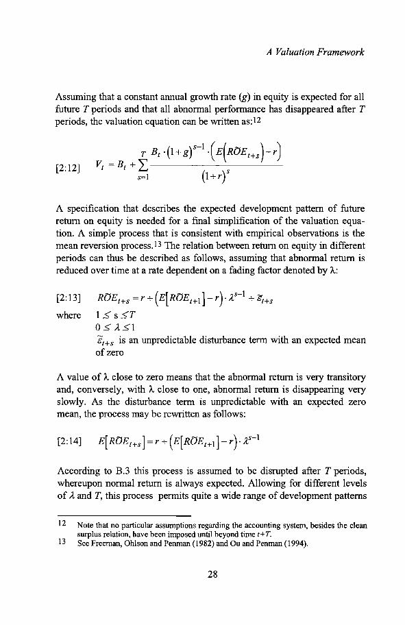
Assuming that a constant annual growth rate (g) in equity is expected for allfuture T periods and that all abnormal performance has disappeared after Tperiods, the valuation equation can be written as: 12
[2: 12]
T Bt .(1+ gt-1-(E(RDEt+s )-r)
Vt == Bt + L----------s=l (1 + r)S
A specification that describes the expected development pattern of futurereturn on equity is needed for a final simplification of the valuation equation. A simple process that is consistent with empirical observations is themean reversion process. 13 The relation between return on equity in differentperiods can thus be described as follows, assuming that abnormal return isreduced over time at a rate dependent on a fading factor denoted by A:
[2: 13] RDEt+s =r+ (E[RDEt+I] - r). ,4s-1 + b"t+s
where 1~ s~T
O~ A~1
8t+s is an unpredictable disturbance term with an expected nleanof zero
A value of Aclose to zero means that the abnormal return is very transitoryand, conversely, with A close to one, abnormal return is disappearing veryslowly. As the disturbance term is unpredictable with an expected zeromean, the process may be rewritten as follows:
[2:14] E[RDEt+s] =r+ (E[RDEt+l] - r). ,4s-1
According to B.3 this process is assumed to be disrupted after T periods,whereupon normal return is always expected. Allowing for different levelsof A and T, this process permits quite a wide range of development patterns
12
13
Note that no particular assumptions regarding the accounting system, besides the cleansurplus relation, have been imposed until beyond time t+T.See Freeman, Ohlson and Penman (1982) and Ou and Penman (1994).
28
Accounting Information and Stock Prices
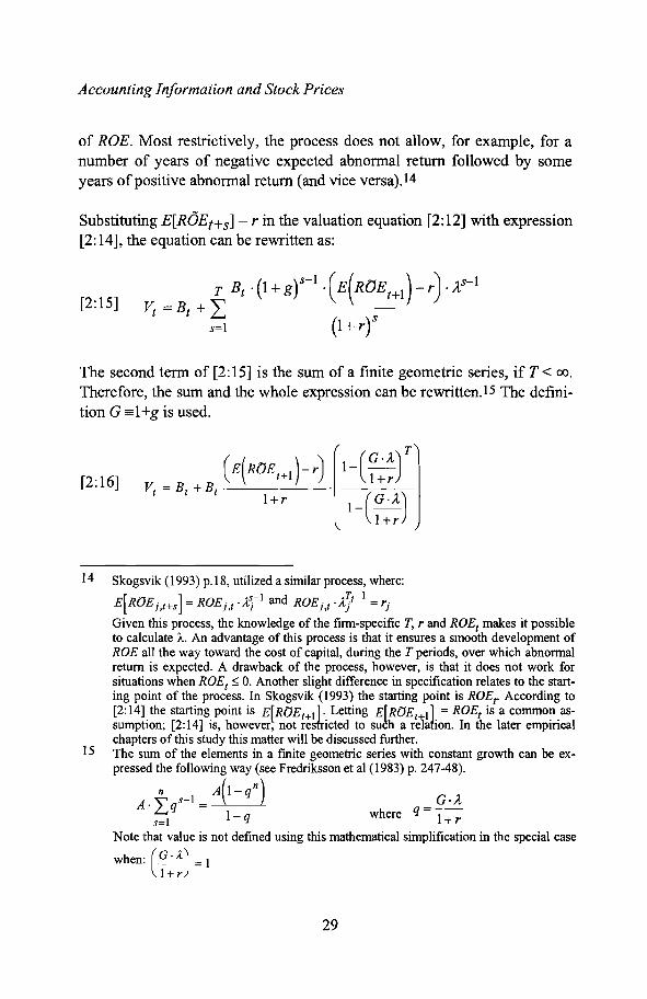
of ROE. Most restrictively, the process does not allow, for example, for anumber of years of negative expected abnormal return followed by someyears ofpositive abnormal return (and vice versa).l4
Substituting E[ROEt+s] - r in the valuation equation [2:12] with expression[2:14], the equation can be rewritten as:
[2: 15]T Bt ·(1+gt-1.(E(ROEt+l)-r).A,S-1
Vt =Bt +I------------s=l (1 + r)S
The second term of [2:15] is the sum ofa finite geometric series, if T< 00.
Therefore, the sum and the whole expression can be rewritten. 15 The definition G ==1+g is used.
[2: 16]
l_(G ..,1,) T
l+r
l_(G ..,1,)l+r
14
15
Skogsvik (1993) p.18, utilized a similar process, where:
[ ]s-1 d T·-1E ROEj,t+s = ROEj,t .A:,j an ROEj,t 'Aj) = rj
Given this process, the knowledge of the firm-specific T, r and ROEt makes it possibleto calculate A. An advantage of this process is that it ensures a smooth development ofROE all the way toward the cost of capital, during the T periods, over which abnormalreturn is expected. A drawback of the process, however, is that it does not work forsituations when ROEt ~ O. Another slight difference in specification relates to the starting point of the process. In Skogsvik (1993) the starting point is ROEt . According to[2:14] the starting point is E[ROEt+11. Letting EfROEt 11= ROEt is a common assunlption; [2: 14] is, however, not resh-icted to su~h a reiafion. In the later empiricalchapters of this study this matter will be discussed further.The sum of the elements in a finite geometric series with constant growth can be expressed the following way (see Fredriksson et al (1983) p. 247-48).
A.~ s-l = A(I- qn) _G·A.~q l-q where q- l+r
Note that value is not defined using this mathematical simplification in the special case
when: (G'A) =1l+r
29

A Valuation Framework
Value is now described as the sunl of two elements: i) the level of currentaccounting equity, ii) the present value of all abnormal profits that the firmis expected to generate from time t to a date T periods ahead. The latter element has in tum been reduced to a multiple of three factors: i) the level ofcurrent accounting equity, ii) next period's expected abnormal return(discounted one period), and iii) a combined factor that depends on a combination of the expected growth, the development pattern and persistence ofabnormal performance, and the discount rate.
The validity of this specification hinges particularly on two critical assumptions. Is it reasonable to assume that abnormal return has disappeared after Tperiods, and is it reasonable to assume that the calculation of the owner'sequity according to the employed accounting convention actually generatesan expected value of JJt+T that equals the expected value of P';+T? Given alarge value of T, the first assumption is probably reasonable for most typesof firms. The second assumption, however, seems more questionable forseveral types of business activities when described by a traditional costbased prudent accounting regime.
30

Accounting Information and Stock Prices
2.3 The valuation model given a prudent accountingregime
The stage when E[Bt+T ] equals E[t';+T] may never occur, even if a firm isonly expected to generate a return that just covers the cost of capital. Forexanlple, for a firm that continuously 'invests' in R&D and where theseinvestments are immediately treated as expenses, this state is unlikely everto occur. Johansson and Ostman (1995) have shown that given rather strictassumptions regarding the investnlent pattern and a constant inflation rate, aconstant relative measurement bias due to different kinds of matching errorscan be expected. An analysis of the size and development of different measurement biases assuming more realistic conditions quickly becomes extremely complex. 16 Simplifications must therefore be made. In this studythe valuation equation will only be expanded to allow for a constant relativemeasurement bias. Assume that the following holds for a prudent (biased)accounting convention. Superscript (b) is introduced to indicate biased accounting:
A.3 The accounting relative measurement bias is expected to be constantover time, in the sense that the fraction of the unbiased equity to thebiased equity is constant over time.
[2: 17] [Bt(U) ]= [Bt~~]
E (b) E (b)Bt Bt+s
for all s ~ 1
This assumption is equivalent to stating that the third counter balancingerror theorem in Johansson and Ostman (1995) holds. 17 An implication ofA.3 is that the growth rate of unbiased and biased equity is the same.Assume further that it is possible to assess the expected level of the permanent measurement bias (denoted PMB) given knowledge of the (biased) accounting regime and the type of assets and liabilities that a particular firm is
16 See Johansson and Ostman (1995) Chapters 8 and 9.17 Note that this is a rather strong assumption. For example, to assume that
E[Bt~~]- E[Bt~~+m] for all m~ 1Bt~~ - Bt~km
would be a less restrictive and possibly a more realistic assumption. However, in orderto achieve a simple model suitable for large-scale empirical testing, the stronger assumption will be utilized in this study.
31
A Valuation Framework
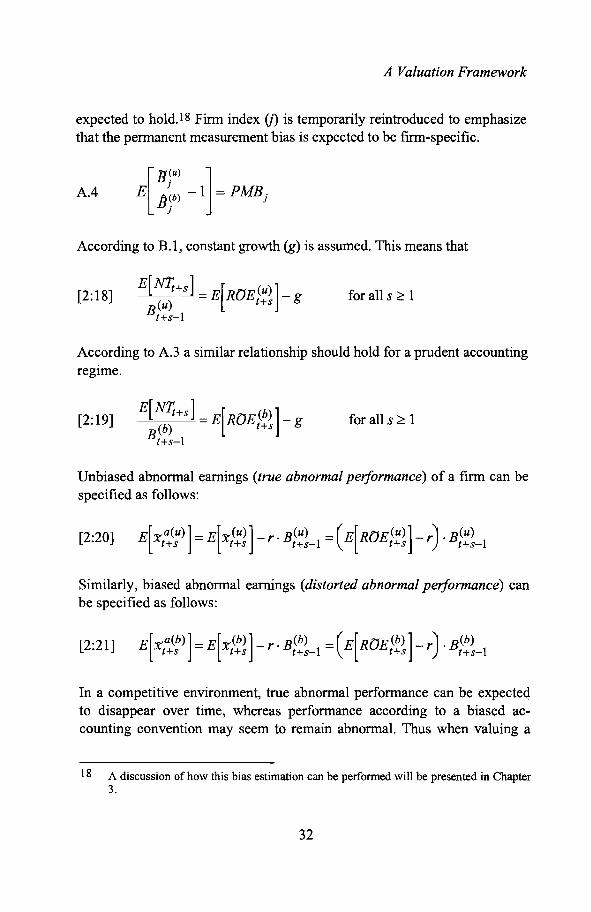
expected to hold. 18 Firm index (j) is temporarily reintroduced to emphasizethat the permanent measurement bias is expected to be firm-specific.
A.4 [l1~U) ]
E bjb) -1 = PMB j
According to B.l, constant growth (g) is assumed. This means that
[2:18] E[N1;+s] =E[ROE(U)]-(u) t+s g
Bt+s- 1
for all s ~ 1
According to A.3 a similar relationship should hold for a prudent accountingregime.
[2:19]E[NT; ]-------"'--_t+---'-"-s =E[ROE(b)]-
B(b) t+s gt+s-l
for all s ~ 1
Unbiased abnormal earnings (true abnormal performance) of a firm can bespecified as follows:
[2:20] E[X-a(U)] =E[X-(U)] - r.B(u) =(E[ROE(U)] - r) .B(u)t+s t+s t+s-l t+s t+s-l
Similarly, biased abnormal earnings (distorted abnormal performance) canbe specified as follows:
[2:21] E[X-a(b)] =E[X-(b)] - r· B(b) =(E[ROE(b)] - r) .B(b)t+s t+s t+s-l t+s t+s-l
In a competitive environment, true abnormal performance can be expecteqto disappear over time, whereas performance according to a biased accounting convention may seem to remain abnormal. Thus when valuing a
18 A discussion of how this bias estimation can be performed will be presented in Chapter3.
32

Accounting Information and Stock Prices
company described by a biased accounting convention, it is important tosucceed in disentangling the part of performance that is pressured by competitive forces. The difference between true and distorted abnormal performance will be a function of the size of the book value of equity, the sizeof the permanent measurement bias (PMB), the rate of growth in the absolute measurement bias (gMB), and the discount rate. Using equations [2:1821] this difference can be formulated as follows:
[2:22] E[:t'.a(b)] _ E[:ra(U)] = (r - gMB). B(b) · PMBt+s t+s t+s-1 t+s-1
According to B.l and A.3, both g and the PMB are constant from timet+1. 19 This means that under these conditions, the difference between trueand distorted abnormal performance will only be a function of the size ofthe book value of equity and a constant, call the constant y:
[2:23]
[2:24]
E[:ra(b)]_E[:ra(U)]=B(b) ·rt+s t+s t+s-1
where
r =(r- g). PMB
Provided that the 'true' abnormal performance that a firm is expected togenerate is unrelated to how performance actually is described, unbiasedabnormal earnings can be extracted from a biased description as follows:
[2:25]( E[ROE(b)] - r) ·B(b) - r ·B(b) =
t+s t+s-l t+s-l
( E[ROE(U)] - r) .B(u) = E[X--a(U)]t+s t+s-l t+s
for all s ~ 1
19 The common tendency to over-value the liability deferred taxes is an example of aparticular accounting issue that can create a measurement bias. As the size of a company's deferred tax might to some extent be a function of the conlpany's level of abnormal performance, the simultaneous assumption of complete permanence in the sizeof the relative measurenlent bias and presence of diminishing abnormal performancecan related to this particular case be viewed as being somewhat inconsistent.
33

A Valuation Framework
The relationship between unbiased and biased ROE can further be specifiedas follows:
B(u)[2:26] E[ROE(b)] =r+ r + (E[ROE(U)] - r). t+s-l for all s ~ 1
t+s t+s B(b)t+s-l
or
[2:27]B(b)
E[ROE(U)] =r + (E[ROE(b)] - r - r). t+s-lt+s t+s (u)
Bt+s- 1
for all s ~ 1
These expressions can be rewritten to:
[2:28] B(b) . (E[ROE(b)] - r- r) =B(u) . ([ROE(U)] - r)t+s-l t+s t+s-l t+s
rplus the cost of equity capital can thus be viewed as the increased hurdlerate which biased ROE must exceed (scaled against biased equity) in orderfor the firm to perform beyond the 'norm', (the norm being unbiased abnormal earnings of zero).
When all expected abnormal performance is expected to have disappeared(after time t+T), [2:26] is obviously reduced to:
[2:29] E(ROE~~+m) =r + r for all m ~ 1
This means that when no abnormal performance is expected (beyond timet+Taccording to B.3) the relationship is simply:
r =E[ROE~km ]- E[ROE~km ]=
[2:30] = E[N1;+T+m] _ E[N1;+T+m]B(b) B(u)
t+T+m-l t+T+m-l
for all m ~ 1
The size and determinants of the constant annual return measurement bias(y), under the conditions of constant growth, a constant relative measure-
34

Accounting Information and Stock Prices
ment bias, and no abnormal performance have previously been derived inSkogsvik (1993, pp. 28).20
A ROE development process similar to [2:14] and consistent with this kindofbiased accounting can be described as follows:
[2:31] E[ROE~~] =r+ r + (E[ROE~~] - (r + r)) ·ls-l
where 1 s ssTOs Aslr = PMB· (r - g)
Given this ROE development process, a known and constant PMB, a knownand constant growth (g), and assuming that all abnormal performance hasdisappeared after T periods, the valuation equation [2: 16] can be extendedto:
[2:32]
20[ (U)] ~N1;+T+ml_ [ (b)] ~N1;+T+ml_
E R()Et+T+m - B(U) - E R()Et+T+m - B(b) - gt+T+m-l t+T+m-l
E[R()E(b) ] _ E[R()E(U) ] = ~N1;+T+m 1_~N1;+T+m1 .Ast+T+m t+T+m Bt~~+m-l Bt~~+m-l
~N1;+T+m] Bt~~+m-l _ E[ N1;+T+m] we haveBt~~+m-l . Bt~~+m-l - Bt~km-l '
35

A Valuation Framework
Value is again described as the sum of two terms: i) the level of current accounting equity adjusted for any measurement bias of the accounting regime, and ii) the present value of all abnormal profits that the firm is expected to generate from time t to a date T periods ahead. The hurdle rate tocalculate abnormal profits has now been adjusted to incorporate the annualn1easurement bias, y.
Dividing both sides of the equation by owners' equity and deducting 1 fromeach side, the following equation is generated:
[2:33]
v: (E(ROE~n-r-r)-t--l=PMB+ .R(b) l+r
t
1- (G. A) T
l+r
l_(G.A)l+r
Within this valuation framework, the following main forces influencing theeconon1ic-to-accounting value relation are thus expected:
Vt1. (b)-I=PMB
Bt
2. ~-1B(b)t
Vt3. (b)-I
Bt
4.Vt(b)-I
Bt
5.Vt(b)-I
Bt
when no abnormal performance is expected
increases when the PMB increases
increases when E(ROE~~) increases
increases when g, T, or A increases
if E(ROE~l ) > (r +r)decreases when g, T, or A increases
if E(ROE~n«r+r)
36
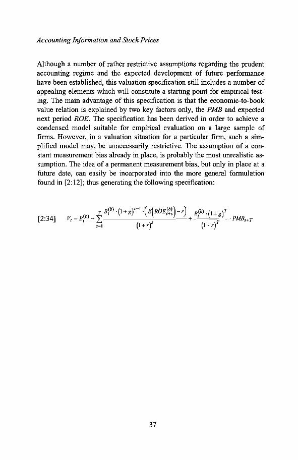
Accounting Information and Stock Prices
Although a number of rather restrictive assumptions regarding the prudentaccounting regime and the expected development of future performancehave been established, this valuation specification still includes a number ofappealing elements which will constitute a starting point for empirical testing. The main advantage of this specification is that the economic-to-bookvalue relation is explained by two key factors only, the PMB and expectednext period ROE. The specification has been derived in order to achieve acondensed model suitable for empirical evaluation on a large sample offirms. However, in a valuation situation for a particular firm, such a simplified model may, be unnecessarily restrictive. The assumption of a constant measurement bias already in place, is probably the most unrealistic assumption. The idea of a permanent measurement bias, but only in place at afuture date, can easily be incorporated into the more general formulationfound in [2: 12]; thus generating the following specification:
[2:34]T B(b) . (1 + g)S-l . (E(ROE(b») - r) B(b) (1 )T
(b) t t+s t . + gVt =Bt + 2: + T ·PMBt+T
s=1 (1 + r)S (1 + r)
37

A Valuation Framework
2.4 A numerical exampleIn the initial valuation framework, economic value was assumed to be afunction of expected future dividends, as in [2: 1]. A number of assumptionsregarding the accounting regime have henceforth been introduced, as well asan assumption of a constant expected growth and a specification of the development of future ROE. To illustrate that the later valuation models in theprevious sections are equivalent to discounted dividend models, a simplenumerical example is presented below.
Basic facts and expectations for a prudent accounting regime:
B(b) = 100 g = 6%0
EO (ROEfb) ) = 30% A = 0.5
r = 10% T = 2
Y = 5% PMB = 1.25
The expected development of equity, ROE, earnings and dividends giventhese expectations are as follows:
s=l s=2 s=3 s=4 s=5 ~ s=oo
B(b) 100 106 112.4 119.1 Constant growth = 6%s-l
EO (ROE}b») 30.0% 22.5% 15.0% 15.0% Constant level = 15%
Earningss 30 23.9 16.9 17.9 Constant growth = 6%
B(b) 106 112.4 119.1 126.4 Constant growth = 6%s
DividendsS 24 17.5 10.1 10.7 Constant growth = 6%
38

Accounting Information and Stock Prices
Discounted dividends according to [2:1]:
10.124 17.5 010-006
V = --+--+. · = 245.2o 1.101 1.102 1.102
The third element in the dividend discount formula is the mathematical simplification that calculates the sum of a perpetual geometric series with constant growth.21
Calculated value according to [2:32]:
_ (1.06. 0.5)2
( ) (0.30 - 0.10 - 0.05) 1 1.10
Vo =100· 1+ 1.25 + 100 · · =1.10 1- ( 1.06 ·0.5)
1.10
= 225 + 20.2 = 245.2
21 This part is identical to the valuation model derived by Williams (1938) and laterpopularized by Gordon (1959, 1962):
i) The expected growth in dividends (g) is constant and eternal (T~oo).ii) The required rate of interest (r) is constant over time.iii) g < r
39
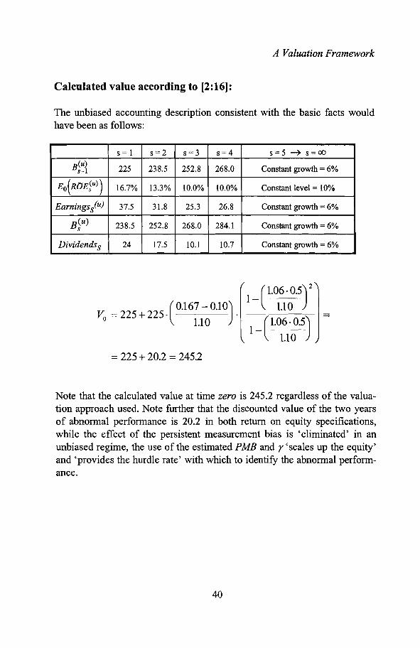
A Valuation Framework
Calculated value according to [2:16]:
The unbiased accounting description consistent with the basic facts wouldhave been as follows:
s=1 s=2 s=3 s=4 s=5 ~ s=OO
B(u)225 238.5 252.8 268.0 Constant growth = 6%s-1
EO(ROE}U) ) 16.7% 13.3% 10.0% 10.0% Constant level = 10%
Earningss(u) 37.5 31.8 25.3 26.8 Constant growth = 6%
B(u) 238.5 252.8 268.0 284.1 Constant growth = 6%s
Dividendss 24 17.5 10.1 10.7 Constant growth = 6%
_ (1.06. 0.5) 2
(0.167 - 0.10) 1 1.10
V == 225 + 225 · · =o 1.10 1- (1.06. 0.5)
1.10
== 225 + 20.2 == 245.2
Note that the calculated value at time zero is 245.2 regardless of the valuation approach used. Note further that the discounted value of the two yearsof abnormal performance is 20.2 in both return on equity specifications,while the effect of the persistent measurement bias is 'eliminated' in anunbiased regime, the use of the estimated PMB and r 'scales up the equity'and 'provides the hurdle rate' with which to identify the abnormal performance.
40

Accounting Information and Stock Prices
2.5 The valuation model in empirical testsAssuming that the valuation models derived in the previous section constitute a reasonable description of the valuation process, it is possible to exchange Mt for Vt in the valuation model.
It is common practice in capital market research to add a risk premium to anestimated risk-free rate of interest in order to allow for uncertainty and riskaverse investors. Ohlson (1995), however, states that it is by no means obvious that risk can be properly captured by simply increasing the discountfactor in a 'present-value-of-expected-dividend' model, such as [2:1] in thisstudy. As a theoretically more appealing alternative, Ohlson (ibid.) refers tothe work of Rubinstein (1976), where adjustments for risk are performed onthe flows (creating certainty-equivalents) rather than on the discount rate.Empirical use of this approach seems, however, to be limited. Ohlson (ibid.p. 31) notes that the risk premium adjusted discount rate concept should beadequate in many empirical applications (or evaluations) of the valuationmodel.
For the empirical tests that will be performed in this study, the idea of anestimated cost of equity capital as the sum of the risk-free interest rate and arisk premium will thus be relied upon, and r will simply be replaced by p inthe valuation equations.
C.2 P = r + risk premium
Exchanging Mt for Vt in the valuation model [2:33], an equation is obtainedin which the Inarket-to-book-value premium is explained by the expectedmeasurement bias and the expected future accounting performance.22
22 The market-to-book value in excess of one will henceforth be called a market-to-bookvalue premiunl. A 'negative premium' may, of course, also occur. Such a 'premium'should, however, more correctly be referred to as a market-to-book value discount.
41

A Valuation Framework
[2:35]
1- (G. AJ T1+r
1-(G.lJ1+r
The first element of this formula is an expression for the expected futureaccounting measurement bias. It has already been given the namePermanent Measurement Bias (PMB).The second element of this formulaconsists of two parts: i) next period's expected abnormal return discountedback one period, ii) a factor that depends on a combination of expectedgrowth, the development pattern and the persistence of future accountingperformance. Let the first part be called Expected Residual Return, orE[RR], and the second part Equity Growth Earnings Persistence Factor, orGPF. Thus:
[2:36]
[2:37] GPF==
1_(GoAJT1+p
1-(G.AJ1+p
Rewriting [2:35] using these expressions and still suppressing the firm index(j), the following model is obviously obtained:
[2:38] ~:) -1 = PMB + GPF· E(RRI+JBt
The relationship according to equation [2:38] can be illustrated graphicallyas in figure 2.1 below. In the absence of an expected persistent accountingmeasurement bias, market-to-book value can be drawn as a positive functionof expected future residual return that goes through the origin and where the
42

Accounting Information and Stock Prices
slope of the line depends on the level of the GPF. The dotted line has beenshifted upwards due to an arbitrary expected existence of a positive accounting measurement bias.
,The slope depends on the GPF
The shift is due to an expected PMB
~ Figure 2.1 A graphical illustration of the relationship between market-to-bookvalues and expected residual return according to equation [2:38].
43

A Valuation Framework
2.5.1 Regression specifications for value level studiesThe explanatory power of the value level specification [2:38] can be assessed for a sample of firms using a linear regression model. For a sampleof firms for which unbiased accounting is possible to obtain, or for whichonly a very small permanent measurement bias is expected, a univariatemodel can be used.
M.1 ~~'t -1=a+A .Et[RRj ,t+l]+&j,tj,t
The inclusion of an estimated expected accounting measurement bias generates the following multiple regression model:23
M.2 ~~'t -1 = a +A ·Et[RRj ,t+l] +~ · PMBj + &j,tj,t
Given a good estimate of the firm's specific expected residual return and thepermanent accounting measurement bias, and given that the valuation modelis valid, the following regression coefficients are expected:
a =0
PI '?- 1P2 = 1
a is expected to be zero as the regression line is expected to run through theorigin. PI is an estimate of the growth persistence factor. The smallestvalue the GPF can amount to, with either A or T amounting to zero, is one.This is in the case of completely transitory abnormal return. Other combinations of the GPF components generate values exceeding one. This meansthat the GPF is expected to be positive and equal or exceed one. P2 is expected to equal one acknowledging the measurement bias. In order to receive a high explanatory power, it is important that the sample of firms isreasonably similar with regard to the level of the growth persistence factor.
23 Viewing M.l as a 'simpler' version of M.2, the added explanatory variable (the PMB)is written last in the expression, in contrast to how it was written in [2:38].
44

Accounting Information and Stock Prices
Consider the following example. Assume access to observations from threedifferent industries, industry A, Band C. Industry A is mature and competitive. Industry B is comparable to industry A, but due to prudence, the specific type of assets that B's firms tend to hold will permanently be undervalued. Industry C is growing quickly and has high barriers to entry. In figure 2.2 a few idealized firm observations from each industry have beenplotted. If these observations were run together in a linear regression analysi~ as outlined in M.l above (without controlling for differences in the accounting measurement bias), a would exceed zero and PI would be positive. If it were possible to estimate and include the measurement bias parameter in the regression, and/or separate the firms into different regressions, it is obvious that the total explanatory power (R2) would increase andthe resulting level of the separate regression coefficients would be different.These observations point to some of the statistical problems associated withthe use of very heterogeneous samples of firms and a rather simple statistical model.
---x- -
Figure 2.2 A graphical illustration of idealized firms' observations from threedifferent industries: A, Band C.
45

A Valuation Framework
2.5.2 Model and regression specifications for value changestudies
Using valuation equation [2:32], the abbreviations introduced in Section 2.3,and assuming a constant expected GPF and PMB, the valuation formula canbe written as follows:
[2:39]
A 'value change model' can either attempt to explain capital gain alone orcapital gain plus dividends (total return). Relative capital gain and rate ofreturn for one period can be specified as follows:
[2:40]
[2:41]
Capital gaint+l = Mt+l - Mt
M t
RMt+l - Mt + Dt+1 - Nt+1etumt+l == ----....:..._-----
M t
Moving s periods ahead, [2:39] can be expressed as:24
[2:39'] M t+s == Bt+s + Bt+s . Et+s(RRt+s+l)' GPF + Bt+s · PMB
A value change version of [2:39] can thus be written as follows:
M t+s - M t == Bt+s - Bt +
[2:42] + [Bt+s .Et+s(RRt+s+I)-Bt ·Et(RRt+I)]. GPF+
+ [Bt+s - Bt ] · PMB
According to this specification, the chal1ge in market value can be explainedby three components: i) the change in accounting equity, which according tothe clean surplus relation is equal to earnings adjusted for net transactions
24 The assumption of a constant GPF implies that the components of the GPF (1, g and p)are constant and that either T is so large that the effect of moving closer to the horizonis marginal or that the horizon keeps nloving forward. This is obviously a set of ratherrestrictive assumptions.
46

Accounting Information and Stock Prices
with the owners, ii) the change in expectations conc(,ming the firm's abilityto generate abnormal eamings25 times the GPF, and iii) the change in accounting equity times the expected persistent accounting measurenlent bias.In the absence of any accounting measurement biases and any expected abnormal performance, the change model simply collapses to an equality between change in equity and change in market value. Dividing both sides ofsuch an equality with opening period market value, a benchmark regressionmodel consistent with zero expected abnormal performance and no measurement bias is obtained:
M.3 M j,t+s - M j,t B j,t+s - B j,t------ =a + Cl . + ~j,t+s
Mj,t Mj,t
This specification is identical to the one evaluated in Ohlson and Penman(1992), provided that the clean surplus relation of accounting holds.26 Thespecification tested in Easton, Harris and Ohlson (1992) was also similar,except that they included the accumulated value of paid dividends in bothvariables (in their main value change specification).27
Dividing both sides of [2:42] by Mt and rearranging the terms somewhatgenerates a more complete value change model:
2526
27
A discussion ofhow this n1easure can be interpreted will follow later.They used (accumulated) net earnings per share minus (accumulated) dividends pershare instead of change in equity.M.3 could in principle be run either on full market value or on a per share basis. In theabsence of any new issues of shares and given appropriate adjustment for stock splitsand stock dividends, both specifications will generate identical results. A new issuewill, however, result in a simultaneous boost in both aggregate market value and equity.On a per share basis, the new issue (adjusted for any element of a stock dividend)should, however, result in no change in the share price. Given the focus on the relationbetween (retained) value creation as it is described by the accounting language and howit is perceived by the investors (manifested in a share price), an analysis on a per sharebasis will provide a stronger test. With frequent occurrences of large new issues, themarket value specification would be positively biased. Both Easton, Harris and Ohlson(1992) and Ohlson and Penman (1992) ran their similar regressions on a per sharebasis.
47

[2:43]
A Valuation Framework
Mt+s - Mt =(1+ PMB). Bt+s -Bt +M t M t
+ GPF. [£t+s(~+s+I) - £t (1~Tr+l)]M t
where Et+s(~+s+l)=Bt+s . Et+s(RRt+s+l) and RI is short for residual
income.
[2:43] is obviously a capital gain specification. The validity of this nlodelcan be tested empirically through regression analysis in the following way:
M.4
This specification is quite similar to one of the specifications tested inEaston and Harris (1991). They attempted to explain one year's market return, with net income and change in net income normalized with openingmarket price. The estimated regression coefficient of the variable 'change innet income' has been analyzed in several market-based accounting studies,for example in Lev (1989). The regression coefficient has often been calledthe Earnings Response Coefficient (ERC) in the literature. In Easton andHarris (1991), the main motive for running the multivariate regression appears to have been to evaluate which of the two variables best explains returns, viewing tIle two variables more or less as competitors.28 In this study,the two variables are viewed as complimentary variables, rather thancompetitors. The change in equity variable is viewed as an attempt to measure the value created (and retained), while the change in the expected residual income variable is interpreted as an indicator (or signal) of changes inthe expected ability of the firm to perform. Given good estimates of the firmspecific residual income and given that the assumptions of constant GPFs
28 The origin of such a competitive view can presumably be traced back to the empiricalresearch that followed Ball and Brown (1968).
48

Accounting Information and Stock Prices
and PMBs are reasonably valid, the following regression coefficients can beexpected: tl is expected to be zero, and el is expected to equal one in theabsence of an accounting measurement bias. In a certain sample, for example research and development intensive firms described by a conservativeaccounting regime, el' however, is expected to exceed one. e2 is an estimate of the growth persistence factor. Thus the coefficient can be interpreted, for example, as an estimate of how long a firm can be expected todefend a new performance level. The e2 coefficient is expected to be positive and to be equal to or exceed one. The level, significance and stability ofel can indicate how well the accounting convention's description of thefirm's value creation is translated into changes in the valuation on the stockmarket. Using published accounting data to estimate expected values of RI,the level, significance and stability of e2 can indicate the strength and relevance of this accounting signal of the firm's ability to generate value.
This signal perspective is quite similar to the classical setting of 'goodnews' versus 'bad news' in the Ball and Brown type of analysis. In that lineof studies, unexpected return has generally been explained by unexp'ectedearnings. The standard operationalization of unexpected earnings as changein published earnings per share (minus a drift term) is similar to the changein expected RI variable of this study in a one-year change setting, providedthat actual ROE is used as a base for expectations, the cost of capital is constant over time, and the growth in equity capital (due to retained earnings) isviewed as the reason for a drift term.
Finally, with explicit firm-specific estimates of the PMB, one may alsospecify the following multivariate regression:
M.5
3 Runsten
MJO t+s - MJo t RJo t+s - RJo t, , == a +cl·' , +
MOt MotJ, J,
[Et+s(RIj,t+s+l) - Et(RIj,t+l)]+~. +
M'tJ,
(Bj,t+s - Bj,t). PMB+ c3 . + '8j t+s
M't 'J,
49

A Valuation Framework
el is now expected to equal one and e3 is expected to 'pick up' differencesin the permanent accounting measurement bias.
Questions to address within this proposed framework relate to the association of the accounting language's descriptions of value creation with valuecreation as perceived by the market (manifested in changes in share prices).As noted earlier, regression specifications similar to M.3 have previouslybeen tested on US data for both long and short intervals (three months up to20 years).29 These studies all noted a stronger association, in an R2 sense, asthe time interval was prolonged. A comnlon conclusion has been that themore backward looking value creation descriptions of traditional accountingalign better with the forward looking (expectation-based) value creationdescriptions, calculated from the changes in market prices, when longerintervals are studied. This result has been attributed to the fact that the likelihood of accounting descriptions describing the same value created as thevalue created perceived by the market, increases as the time horizon increases, that is, there is more value creation overlap. Warfield and Wild(1992) further noted a difference in association for firms from different industries. They argue that the accounting regime's earnings recognition lag ishigher for industries such as mining, construction and manufacturing compared to industries such as wholesale trade, retail trade and service.
Adding control for changes in earnings expectations, such as in M.4, haspreviously and quite similarly been tested for a one-year change period inEaston and Harris (1991). However, to my knowledge, a variable similar tochange in E[R1] and an extension of the time period have not previouslybeen used.30 Further, controlling for differences in expected firm-specificaccounting nleasurement biases (PMBs) does not appear to have been previously evaluated in a value change setting.
Beyond the three regression specifications and the different time intervalsthat will be tested, this study will also explore the differences in associationrelated to different firm characteristics, changes in the economic climate andsome major changes in the accounting regime.
29
30
Warfield and Wild (1992), Easton, Harris and Ohlson (1992), Ohlson and Penman(1992) and O'Hanlon and Pope (1997). The latter used data from the UK.Easton, Harris and Ohlson (1992) did, however, test the variable change in accumulatedearnings.
50

Accounting Information and Stock Prices
2.5.3 Analysis of the different elements of the regression modelsBefore the regression specifications M.1 to M.5 are empirically tested, eachexplanatory variable in the valuation equations can be further discussed. Important issues regarding each explanatory variable include whether they canbe observed, or estimated, and how they can be expected to vary betweendifferent firms at different tin1es.
• M· tJ'can be observed daily and is thus known at tin1e t.
• B· t'j,is published with a two - four n10nth lag annually, most often describingaccounting value at the end of December each year. The increasedfrequency of interim reports means that more frequent observations areavailable.
• Et[RRt+t]is the next period's expected return on equity minus the market's requiredreturn (adjusted for the accounting measurement bias) discounted back oneperiod (recall formula [2:36] for the full definition). It is crucial to generatean estimate of the next period's expected ROE. Required return (P) at time t
can be estimated as the long-term risk-free interest rate plus a market riskpremillm. If a persistent measurement bias is expected for the firm, thismust also be estimated. Knowledge of different firm characteristics and theaccounting regime is essential for this estin1ate.
• GPFjdepends on a combination of '"A, T, G and p (recall formula [2:37] for the fulldefinition). The size of these paran1eters can largely be expected to be functions of the type of business the firm is involved in and the environment thefirm is operating in. The degree of competitive pressures and barriers toentry is expected to influence the level of '"A and T. Whether the market inwhich the firm is active is mature or has a high growth potential is expectedto influence the level of G. p is essentially a function of the interest rate
51

A Valuation Framework
(which in tum is related to expected inflation) and risk. The level of theGPF is thus expected to vary between different industries, depending on theindustry's current degree of competitiveness and growth potential. To illustrate the combined effect on the value of the GPF of different combinationsof growth and persistence, five tables are presented below. Tables 2.1a-eshow the level of the GPF for different combinations of the growth parameter G and the persistence parameter A" given that T equals 2, 5, 10, 15and 20 years and p is equal to 15%..
Table 2.1a The growth persistence factor (GPF) for T = 2, 5, 10, 15 and 20years and p equal to 15% for different combinations of A, and G.
T=2 AG 0.00 0.10 0.20 0.30 0.40 0.50 0.60 0.70 0.80 0.90 1.000.90 1.0 1.1 1.2 1.2 1.3 1.4 1.5 1.5 1.6 1.7 1.80.95 1.0 1.1 1.2 1.2 1.3 1.4 1.5 1.6 1.7 1.7 1.81.00 1.0 1.1 1.2 1.3 1.3 1.4 1.5 1.6 1.7 1.8 1.91.05 1.0 1.1 1.2 1.3 1.4 1.5 1.5 1.6 1.7 1.8 1.91.10 1.0 1.1 1.2 1.3 1.4 1.5 1.6 1.7 1.8 1.9 2.01.15 1.0 1.1 1.2 1.3 1.4 1.5 1.6 1.7 1.8 1.9 2.01.20 1.0 1.1 1.2 1.3 1.4 1.5 1.6 1.7 1.8 1.9 2.01.25 1.0 1.1 1.2 1.3 1.4 1.5 1.7 1.8 1.9 2.0 2.11.30 1.0 1.1 1.2 1.3 1.5 1.6 1.7 1.8 1.9 2.0 2.1
Table 2.1b
T=5 AG 0.00 0.10 0.20 0.30 0.40 0.50 0.60 0.70 0.80 0.90 1.000.90 1.0 1.1 1.2 1.3 1.5 1.6 1.8 2.1 2.4 2.8 3.20.95 1.0 1.1 1.2 1.3 1.5 1.7 1.9 2.2 2.6 3.0 3.51.00 1.0 1.1 1.2 1.4 1.5 1.7 2.0 2.3 2.8 3.2 3.91.05 1.0 1.1 1.2 1.4 1.6 1.8 2.1 2.5 2.9 3.5 4.21.10 1.0 1.1 1.2 1.4 1.6 1.9 2.2 2.6 3.1 3.8 4.61.15 1.0 1.1 1.2 1.4 1.6 1.9 2.3 2.8 3.4 4.1 5.01.20 1.0 1.1 1.3 1.5 1.7 2.0 2.4 2.9 3.6 4.4 5.51.25 1.0 1.1 1.3 1.5 1.7 2.1 2.5 3.1 3.9 4.8 5.91.30 1.0 1.1 1.3 1.5 1.8 2.2 2.7 3.3 4.1 5.2 6.5
52

Accounting Information and Stock Prices
Table 2.1c
T=10 A,G 0.00 0.10 0.20 0.30 0.40 0.50 0.60 0.70 0.80 0.90 1.00
0.90 1.0 1.1 1.2 1.3 1.5 1.6 1.9 2.2 2.6 3.3 4.20.95 1.0 1.1 1.2 1.3 1.5 1.7 2.0 2.4 2.9 3.7 4.91.00 1.0 1.1 1.2 1.4 1.5 1.8 2.1 2.5 3.2 4.2 5.81.05 1.0 1.1 1.2 1.4 1.6 1.8 2.2 2.7 3.5 4.8 6.91.10 1.0 1.1 1.2 1.4 1.6 1.9 2.3 3.0 4.0 5.6 8.31.15 1.0 1.1 1.2 1.4 1.7 2.0 2.5 3.2 4.5 6.5 10.01.20 1.0 1.1 1.3 1.5 1.7 2.1 2.6 3.5 5.1 7.7 12.21.25 1.0 1.1 1.3 1.5 1.8 2.2 2.8 3.9 5.8 9.1 15.01.30 1.0 1.1 1.3 1.5 1.8 2.3 3.0 4.3 6.6 10.8 18.5
Table 2.1d
T= 15 A,G 0.00 0.10 0.20 0.30 0.40 0.50 0.60 0.70 0.80 0.90 1.00
0.90 1.0 1.1 1.2 1.3 1.5 1.6 1.9 2.2 2.7 3.4 4.50.95 1.0 1.1 1.2 1.3 1.5 1.7 2.0 2.4 2.9 3.9 5.41.00 1.0 1.1 1.2 1.4 1.5 1.8 2.1 2.6 3.3 4.5 6.71.05 1.0 1.1 1.2 1.4 1.6 1.8 2.2 2.8 3.7 5.3 8.61.10 1.0 1.1 1.2 1.4 1.6 1.9 2.3 3.0 4.2 6.4 11.21.15 1.0 1.1 1.2 1.4 1.7 2.0 2.5 3.3 4.8 7.9 15.01.20 1.0 1.1 1.3 1.5 1.7 2.1 2.7 3.7 5.6 10.0 20.51.25 1.0 1.1 1.3 1.5 1.8 2.2 2.9 4.1 6.7 12.9 28.71.30 1.0 1.1 1.3 1.5 1.8 2.3 3.1 4.6 8.1 17.0 40.6
Table 2.1e
T=20 A,G 0.00 0.10 0.20 0.30 0.40 0.50 0.60 0.70 0.80 0.90 1.00
0.90 1.0 1.1 1.2 1.3 1.5 1.6 1.9 2.2 2.7 3.4 4.60.95 1.0 1.1 1.2 1.3 1.5 1.7 2.0 2.4 2.9 3.9 5.61.00 1.0 1.1 1.2 1.4 1.5 1.8 2.1 2.6 3.3 4.6 7.21.05 1.0 1.1 1.2 1.4 1.6 1.8 2.2 2.8 3.7 5.5 9.61.10 1.0 1.1 1.2 1.4 1.6 1.9 2.3 3.0 4.2 6.8 13.51.15 1.0 1.1 1.2 1.4 1.7 2.0 2.5 3.3 4.9 8.8 20.01.20 1.0 1.1 1.3 1.5 1.7 2.1 2.7 3.7 5.9 11.7 30.91.25 1.0 1.1 1.3 1.5 1.8 2.2 2.9 4.2 7.2 16.4 49.41.30 1.0 1.1 1.3 1.5 1.8 2.3 3.1 4.7 9.1 23.7 81.4
The GPF varies in the tables from a value of one to values in the region ofeighty when going from a completely transitory abnormal performance (i.e.abnormal performance that immediately fades off after t+1) to a combination oftwel1ty years of constant abnormal performance (i.e. A,=l means that
53

A Valuation Framework
the residual return is constant) on a permanently fast growing equity base. Itis obvious that the latter con1bination is unlikely for most firn1s. One canidentify areas in the tables where the GPF does not change very much. If itwere possible to identify firms, or industries, for which a fairly equivalentlevel of the GPF could be expected, this would be a useful base for the selection of fim1s to be included in different empirical tests.
The competitive forces within an industry have been studied and describedby, for example, Porter (1980). In his terminology, pressure towards normalprofitability can be expected from: current competitors within the industry,potential new entrants, suppliers of goods and labor, the firm's customers,and from potential substituting products. For firms whose competitive edgeis hard to copy, protected via patents or is due to, for example, cost advantages resulting from economies of scale, the reversion process may be expected to be rather slow. For firms currently in a loss situation, the reversionprocess should necessarily be expected to be rather quick if the firm is expected to survive at all. The pressure, especially from investors, may be expected to be strong.31 Consider thus the following potential clusters offirms:
31 There are, however, several examples of firms that for extended time periods havefailed to reach what would be considered a normal level of profitability.
54

Accounting Information and Stock Prices
Table 2.2 A table indicating the relation between different firm and industrycharacteristics and the expected size of the growth persistence factor.
Subgroup Firm/industry Growth persistencecharacteristics factor
• Quick reversion Loss situationCompetitive industry 1~GPF<3Low barriers to entry
• Slow reversion! Barriers to entryNormal growth Mature to normal growth 3 ~GPF~8
• Slow reversion! High barriers to entryHigh growth Rapid expansion GPF> 8
• PMBis expected to be zero when the accounting regime is unbiased. The level ofthe expected measurement bias of a firm's equity is a question of how valueis actually measured and how it should ideally be measured (according to atheoretical ideal such as economic value).32 The prevailing accounting regime in Sweden (as well as in most other Western countries) relies on thenotion of conservatism, with historical cost as a valuation cornerstone andthe realization principle guiding when income may be recognized.Following the recommendations of this kind of an accounting regime,'investments' in different types of assets will be treated differently. Forexample, large expenditures in R&D or in a brandname (through marketing)are generally treated as expenses rather than investments. An accounting description that relies on historical cost as the basis for valuation furthergenerates a measurement bias when a firm holds old and potentially veryvaluable assets. A conservative accounting regime does, furthermore, notnormally allow firms to recognize the potential value of 'investments' inspecialized human resources. Older Swedish accounting practice (relying11eavily on valuation according to what was allowed from the tax authoritiespoint of view) allowed substantial hidden reserves related to, for example,
32 Assuming that such an ideal can actually be defined.
55
A Valuation Framework
the valuation of inventory and depreciable assets. A direct measurement biasis, of course, created by such a non-open accounting procedure, an indirectmeasurement bias is, furthem10re, created by the later common accountingprocedure to value the interest-free deferred tax liability at a face value.
It is thus not difficult to identify characteristics of firms that are prone togenerate a large persistent measurement bias. Such characteristics include:
• Permanent and large R&D expenditures (e.g. pharmaceuticals and 'hightech' firms).
• Permanent and large marketing expenditures (e.g. brandname-intensivefirms).
• Significant investments in specialized human competence through training, etc. (e.g. consulting firms).
• Permanent and large investments in assets with long economic lives (e.g.real estate companies).
• A significant inventory of 011going projects with a long production cycleand a large accumulated income that is reported according to the'con1pleted contract n1ethod' (e.g. construction companies).
Unfortunately, estimating the firm-specific bias is a difficult task. The biasdepends on the firm's combined mix of these types of characteristics, whichin tum depends on factors such as the actual outflow to inflow lag related tothe firm's expenditures (investments). The average economic lives, the agestructure and value change of the assets affects the average unrealizedholding gain. Furthem10re, the inflation rate, changes in the inflation rateand the real growth of the firms will affect the size of the bias.
For firms that do not invest heavily in R&D or marketing, that do not relyon specialized human resources, and whose assets do not have longeconomic lives, the PMB may be expected to be close to zero.
56

3 RESEARCH DESIGN CONSIDERATIONS
In investigating the association between the accounting measures of valueand value creation with stock market prices and price changes, it has beenconsidered important to control for differences in i) firm characteristics, ii)changes in the economic climate, and iii) accounting changes. Some of theseissues will be of particular interest in themselves; others are deemed important to control for in order to avoid the effects of confounding variables.Extreme heterogeneity in a sample of firms, in one or several of thesedimensions, is expected to significantly affect the result of estimating regression specifications, such as M.l to M.5. Low explanatory power andunstable regression coefficients are thus deemed as likely consequences.
3.1 Firm characteristicsConsistent with the outlined valuation model and well-known characteristicsof the traditional cost-based accounting regime, the most important firmcharacteristic is considered to be related to the difference in expected size ofthe accounting measurement bias for different types of business activities.Identification and quantification issues related to this kind of measurementbias will be elaborated on at some length in the next few sections. It is alsoconsidered important to identify characteristics of firms that are expected tohave non-normal growth and experience strong persistence in abnormalperformance, this will be briefly discussed in Section 3.1.2. Finally, ifexpected future ROE is based on the current level of ROE (as in manyprevious earnings-return studies), the identification of firm types for whichsuch a simple estimation procedure may be considered particularly invalid,is deemed important. These matters will briefly be discussed in Section3.1.3.

Accounting Information and Stock Prices
3.1.1 Expected accounting measurement bias (in capital terms)The level of the expected measurement bias of a firm's book value is inprinciple a question of how value is actually measured according to theprevailing accounting regime in comparison with economic ideal measurement principles-eompare to the previously used notion of unbiasedaccounting. The established 'solution' to the problem of describing valueand value creation in a world of uncertainty and non-specified timehorizons, has been to rely on measurement rules based on prudence.Historical cost is the general valuation base and the realization principlegenerally governs when income may be recognized. Thus the accountingregime has a deliberate tendency to realize losses early and gains late, andto valuing assets low and liabilities high. The valuation model used in thisstudy is based on discounted (net) dividends to the owner of the fiml.Conceptually, the ideal measurement principles against which the biasshould be scaled can thus be found in the classical theory of capital value(see, for example, Fisher, 1906 and Lindahl, 1939). According to the notionof unbiased accounting utilized in Chapter 2, accounting value is onlyexpected to equal economic value when no abnormal performance isexpected. Such a valuation concept is most consistent with a current costbased accounting system that allows for capitalization of investments indifferent intangibles. Johansson and Ostman (1995 p. 116) point out(referring to Beaver, 1989) that it is difficult or even impossible to, inpractice, define and measure economic value precisely in a world of uncertainty.I
The prevailing accounting procedures do, nevertheless, in some instances,deviate so much from the ideal reference point that it should be worthwhileto attempt to at least crudely assess the size of the measurement biases.Fruhan (1979) studied the creation, transfer and destruction of shareholdervalue. In order to control for accounting measurement problems, he attempted to nlake systematic adjustments for the measurement biases heidentified as the most significant ones. Fruhan made calculations of bookvalue of equity adjusted for capitalized investments in advertising and R&D.
Johansson and Ostman (1995) further point out that actual measurement principles mayhave a non-trivial influence on actual cash flows, via what they refer to as the postcontracting role of accounting (for example, via tax regulations and debt covenants),and related to the role of motivating and influencing the behavior of users.
58

Research Design Considerations
He further revalued assets according to estimated replacement costs.Fruhan's estin1ates of the accounting measurement bias will be discussedlater.
The size of the measurement bias can be expected to vary immensely fordifferent balance sheet items. As different firms are expected to hold different mixes of balance sheet items, some firms are prone to have large expected permanent measurement biases, whereas others are not.
3.1.1.1 Sources ofthe measurement bias for different balance sheetitems
This section discusses the valuation principles that have generally been usedin Sweden for different balance sheet items, and how these valuation principles are expected to generate deviations from the value norm. The presentation follows the traditional order in which the items have appeared in thebalance sheet. Consider the following simplified balance sheet.
• Cash • Operating liabilities• Accounts receivable • Financial liabilities
• Inventory • Pension obligations
• Other accruals
• Depreciable assets • Untaxed reserves
• Land• Investment in financial assets • Equity
• Other long-term assets...IIntangIbles: IOff-balance sheet lIabIlItIes:
I. Know-How I. Guarantee commitment II r--------------------~_~~E~~~~ J
CashCash is generally valued at face value and does not normally cause anyvaluation problems. If the cash is in a foreign currency, a conservative biasis potentially created via the use of the 'lower of cost or market' valuationrule.
59

Accounting Information and Stock Prices
Accounts receivableAccounts receivable generally causes no large valuation problems. The factthat this asset does not normally generate interest income means that, in astrict sense, it will tend to be overvalued when stated at face value. Thelonger the average collection period and the higher the cost of capital, thelarger this effect is.
Inventory and work in progressThe valuation of inventory in Sweden generally follows the rule of 'lower ofcost or market' and the 'first in first out' principle (FIFO). The FIFO principle ensures that the conservative bias is rather snlall given a reasonablyhigh inventory turnover with low value added.2 Long-term project-intensivecompanies with significant value added (for example, building and construction finns) with revenue recognition at conlpletion nlay, of course, hold'inventory' that is significantly undervalued.
Until 1990, it was for tax purposes possible to value inventory very low.The consequences of this low valuation has, however, been openly disclosed(via full valuation of the asset and a deduction classified as an untaxedreserve between liabilities and equity), at least for the listed Swedishcompanies, since the mid 1960s.3
Other accrualsOther accruals are not generally expected to cause severe valuation problems.
Depreciable assetsDepreciable assets (machinery and equipment, buildings, ships, acquiredgoodwill, etc.) are generally valued at historical cost, reduced by accumulated linear depreciation over the expected economic life. The existence oflarge umealized holding gains may constitute a permanent situation for afirm that holds a portfolio of long lived assets for many years, and either thedepreciation plan is too aggressive and/or there is inflation in the economy(generating nominal value changes in the assets held by the firm). The size
2
3
The unrealized holding gains for a firm trading in commodities with very large pricefluctuations (such as oil or coffee), may however still at times be non-trivial.Open disclosure has been enforced by law since 1977 (ABL 75) and earlier by arecommendations from NBK and FAR. For further details, see Hanner (1980).
60

Research Design Considerations
of the permanent n1easurement bias is expected to be a function of the average age of the assets held and the level of the inflation rate.4
Given constant inflation (equaling the value change of the specific asset), avalid depreciation scheme and knowledge of the economic life of an assettype, the bias of traditional accounting measurement (relative to currentcost) for a portfolio of the asset type can be calculated:
[3:1]N A(r)
Assetbias=I((1+ir- 1)' Ck r(l-1")n=o ace Air)
where
i=
n=A(r) -
n,k -
acc[Ay)] =
r=
the annual rate of change in value for the assettype-in the simplest case corresponding to therate of inflationthe age of the asset (0 years to Nyears)the reported book value of the n year old asset oftype k (after accumulated depreciation)the accumulated book value of all assets of type k(after accumulated depreciation)
the tax rate
The bias for assets of type k (with the same economic life and the same depreciation schedule) is the sum of unrealized holding gains (after tax) for allassets of type k (at a certain date of valuation) divided by the book value ofthese assets (at the same date).
The depreciation rules applicable for taxation purposes have been rathergenerous (for machinery and equipment, a company has a choice between30% depreciation on opening book value or a five-year straight line depreciation of acquisition value). Further, the taxation rules connected to the socalled 'investment funds' could generate a complete write-off of any de-
4 Note that even if a conservative bias is to be expected on average, one may observe theopposite, due to, for example, large declines in property values on the market,combined with the regulations demanding write-downs on fixed assets which have beensubject to value decline.
61

Accounting Information and Stock Prices
preciable asset, even a building, during the investment year.5 Given separatedisclosure of depreciation according to plan and depreciation for taxationpurposes, this causes no additional problems. However, such opendisclosure has not been the general norm until the early 1980s. A gradualadaptation to open disclosure began to occur in the late 1960s. The effect ofthis accounting disclosure issue will be considered separately later in thisstudy.
Land and equivalent propertyLand and equivalent property is generally valued at historical cost. The sizeof the permanent measurement bias is thus expected to be a function of theage of the assets held and the level of annual nominal value change since theacquisition dates.6 To calculate a permanent measurement bias, an estimateof the holding periods and the annual value changes is needed.7
Investments in financial assetsInvestments in shares and otl1er financial assets are generally valued at historical cost. The expected benefits of owning shares are dividends and capital gains. Capital gains remain unrecorded until the shares are sold. The sizeof this measurement bias is thus expected to be a function of the age of theshares and the level of annual nominal capital gains since the acquisitiondates.8
5
6
7
8
The investment fund system first came into being in 1938, but it did not becomeimportant until 1955, when the rules changed. After several revisions, the system wasabandoned in 1990. See, for example, Lodin et at (1990) and Angelin and Jennergren(1994). Note, however, that the effect (the existence of a deferred tax given opendisclosure) of a complete write-off of a long lived asset will remain for many years after1990.Note that Swedish valuation rules allow for write-ups of an asset with a 'substantial andpermanent' market value in excess of acquisition cost. These unrealized holding gainsare, however, not allowed to pass through the income statement and thus violate theclean surplus relation of accounting.The fact that the investment pattern in this type of asset can be expected to beparticularly non-continuous may make the assumption of a permanent measurementbias in this case somewhat dubious.Note that since the mid 1980s in an increasing number of firms the shares held inassociated companies have been valued according to the so-called 'equity-method'.According to this valuation method, the share value will increase in proportion to therealized profits in the associated firm (net of distributed dividends). The expectedmeasurement bias for these firms is thus obviously less important.
62

Research Design Considerations
Intangible assetsInvestments in intangible assets can create a large permanent measurementbias. In a number of companies, large resources are spent annually in orderto generate successful future business. Typical examples of such activitiesare research and development, future-oriented training of personnel, andmarketing campaigns. The resources associated with these activities arecommonly recorded as an immediate expense, rather than being treated asan investment and capitalized. Assuming that an expenditure is expected togenerate a 'fair but late return', the size of the measurenlent bias is a function of how late this return is expected to be realized (and the discount rate).
Consider an investment of a 100 in a zero-coupon bond that repays 161.1five years later. This investment generates 10% annual return and should(given a 10% discount rate) be recorded at 110 at the end of the first year ina balance sheet, according to economic value theory, and then successivelyincrease towards 161.1 over the next four years. Consider an R&D investment with a similar expected cash flow structure. According to commonaccounting practice, R&D expenditures would be valued in the balancesheet at zero for the five years and the benefit of the investment (161.1)would fil1ally show up as revenue at the end of year 5.9 If such aninvestment is made every year, the accumulated unrecorded value canobviously be substantial. For a stable firm that continuously invests in thiskind of an equivalent to a zero-coupon bond, the measurement bias may beexpected to be large and pennanent. The component that shows up annuallyin the income statement can formally be expressed as:
[3:2] Income component =[I. (1 + r *)h ] - I
where
I = the annual constant investment in real terms (expenditure)r* = a discount rate (expected real return)h = the number of years until the investment pays off
9 It is, of course, somewhat unrealistic to assume that the benefit of an R&D investmentcomes in a one-time lump sum (unless the 'research results' are sold off to a thirdparty). The key point to illustrate, however, is the general effect of a timelag betweeninvestment and harvest.
63

Accounting Information and Stock Prices
The unrecorded value of a constant stock (in real terms) of annual investments in such zero-coupon bond equivalents can then be expressed as:
[3:3][{l+r*)h -1]
Value == I .----r*
The annual expenditures (investments) have for tax purposes been fullytreated as expenses. The tax rate times the unrecorded value can thus beviewed as a deferred tax, implying that the after-tax unrecorded value can beexpressed as follows: 10
[3:4][{l+r*)h -1]
Value == I . . (I - ,)r*
where,= the tax rate
If the annual expenditure in an intangible asset is assumed to have grownannually at a constant rate (8), the bias expression can simply be extendedto: 11
[3:4'][1-(!i5r]
Value = I · 1_ ( 1+ r *) ·(1 - T)
1+0where8 = annual real growth in the expenditure I
The expected investment-to-harvest timelag can be expected to varyimmensely between different enterprises. Typical extreme examples includethe basic research activities in a pharmaceutical company and the marketing
10 The complications introduced by non-zero inflation and a particular set of taxation rulesare not elaborated on here.
11 Note that the measurement bias given this specification will always be smaller givenpositive historical growth (8) 0).
64

Research Design Considerations
campaign for a new shampoo of a consumer goods firm. The zero-couponbond metaphor may be non-representative of a typical project; a companymay invest in a particular project for a nunlber of years and then later alsoharvest for several years. However, for a company that is expected to have abalanced portfolio of ongoing projects, an estimate an average investmentto-harvest timelag and the use of the proposed metaphor may constitute auseful tool to estimate a firm's expected permanent measurement bias.12
The calculation of the measurement bias related to intangibles presentedabove is in spirit similar to, for example, Fruhan (1979). However, Fruhanassumed a regular depreciation scheme for the investments (linear for R&Dexpenditures and the double declining balance method for advertisingexpenditures). The measurement bias calculated with the zero-coupon bondmethod will be larger than the corresponding bias for a linear depreciationplan. This is not surprising as the assets are assumed to increase annually invalue according to the former model and decrease in value according thelatter. Which valuation method that is the most representative is eventuallyan empirical matter.
Operating liabilitiesOperating liabilities are generally valued at face value and do not generallycarry an explicit (and separable) interest cost. This generates a conservativebias (over-valuation of the liability) opposite to the one discussed regardingaccounts receivable. 13 For most firms, however, the relative size of this biasis not expected to be severe. For a finn that permanently tends to generatelarge advance payments from customers, this may, on the other hand, stillgenerate a significant bias.
12
13
Green, Stark and Thomas (1996) used similar reasoning when interpreting theregression coefficient of R&D expenditures. They ran a regression using R&Dexpenditures (deflated by the firm's book value of equity) as an explanatory variablefor the market-to-book value premium on UK data.If the liability is assumed to carry an implicit cost of interest (included in the contractedtransaction price), the face value of the liability includes the expected interest cost andthus still over-states the value of the liability in economical value terms until the daythe debt is repaid. This situation also implies that an interest expense is wrongly labeledacquisition expense and it might also be allocated to the wrong period.
65

Accounting Information and Stock Prices
Financial liabilitiesFinancial liabilities are generally valued according to the face value of thecontractual obligation. As long as these commitments also include paymentof interest rates close to the market rate, a valuation method of this kindcauses no measurement bias. However, fluctuating market interest rates anda firm choosing long-term financing with fixed interest rates can generate ameasurement bias compared to the economic value ideal. A conservativebias related to liabilities in a foreign currency, similar to the previouslydiscussed bias regarding liquid assets, may also occur.
Pension obligationsIn Swedish financial statements, the liability to pay future pensions to present and former employees is comnl0nly valued according an actuarialmodel. Pension obligations are generally long-term, and contingent on uncertain factors such as the life spans of the employees. The valuation of suchobligations is thus necessarily very complex. Skogsvik (1993b), performed adeductive analysis of the measurement bias of a commonly used (inSweden) actuarial model conlpared to a valuation based on economictheory. His conclusions indicate that (given stated assumptions), the size ofthe bias is related to the personnel characteristics of the company, the taxrate and the inflation rate of the economy. The relative over-statement of thepension liability is shown to be most substantial if the company'semployees are young, the tax rate is high, and the future inflation rates areexpected to be high. 14 Further, the measurement bias is shown to be muchsmaller for a company with a predominance of old employees, or with anevenly dispersed age distribution of employees. 1S As companies withpredominantly young enlployees may be expected to have a rather smalltotal pension obligation, the overall measurement bias in relation to thebook value of shareholder equity may not be so severe for most companies.
Untaxed reservesAccording to the Swedish accounting tradition, firms have generally disclosed 'untaxed reserves' as an item between liabilities and equity. Formany firms, this item has amounted to a significant portion of the liabilityside of the balance sheet. The individual user of the information has then
14 See Skogsvik, 1993b p. 39.15 Ibid. p. 39.
66

Research Design Considerations
often chosen to reclassify a part of the untaxed reserves as deferred taxesand the other as owners' equity. The standard method has been to use theprevailing marginal tax rate (or a similar approximation) to accomplish thisseparation. As these tax liabilities do not carry an explicit interest cost andare commonly expected to be paid out several years ahead, the value of theliability tends to be over-stated. If deferred taxes related to unrealized holding gains are calculated in a similar fashion, a corresponding type of overstatement will be present. A valuation approach in the spirit of economicvaluation theory would calculate the liability as the discounted value of expected future tax paymel1ts related to the reversal of the untaxed reservesand the unrealized holding gains. 16 The expected size of this bias is thus afunction of the tax rate, the expected lives of the individual untaxed reserves, the time until unrealized holding gains are realized, and the discountrate. Formally, the expected bias may be calculated as follows:
[3:5]
f ~URt· 'l' + f ~UHGt · 'l'
t=1 (1 + rd,atr t=1 (1 + rd,atrDeferred tax biaso =- - 1
(URo+UHGo)·'
where
,=rd,at=
the change in untaxed reserves at time t
the change in unrealized holding gain at time t
the tax rate
the cost of debt after tax
Book value of equityBook value of equity is calculated as a residual: total assets minus total liabilities. G-iven that all potential measurement errors related to assets andliabilities could be estimated, these errors can in principle be aggregatedinto a total measurement error in equity.
16 See discussion in Skogsvik (1987, pp. 127)
67

Accounting Information and Stock Prices
Off-balance sheet liabilitiesProvided that the accounting regime is guided by conservatism, one doesnot expect any unrecorded off-balance sheet liabilities. However, as suchcases may nevertheless occur, the issue should be mentioned.
Other accounting issuesThis list of measurement issues related to different balance sheet itemscould be supplemented with other accounting issues that may have an effecton the size of the measuren1ent bias. An obvious example of such an issue isthe method used for group consolidation after an acquisition. The poolingmethod17 'preserves' any measurement biases whereas the purchasemethod means that acquired tangible assets are given new current valuesand intangible assets, related to, for example, brandnames and know-how,are capitalized (often under the heading goodwill). The previous discussionof measurement errors has essentially been from the perspective of firmsholding 'balanced portfolios' of assets in terms of age structure and valuechange. Such a balance is obviously, at least temporarily, disturbed after alarge acquisition which is consolidated according to the purchase method. 18
3.1.1.2 Principal estimation procedure ofthe measurement bias
A number of potential sources for a measurement bias were identifiedabove. The size of the measuren1ent problems can be expected to vary between different balance sheet items. The total relative measurement bias of afirm in a particular industry is thus expected to be a function of the types ofassets, intangibles and liabilities that the firm is holding. To estimate afirm's measurement bias in relation to the book value of equity, a three-stepapproach can be used: i) estimate the relative measurement bias of differentitems, ii) identify the relative importance of each item for the firm, and iii)scale and aggregate these errors against the book value of equity.
The following formula is a comprehensive way to illustrate a procedure ofthis kind.
17
18
A method similar to the pooling method (called 'Parivardemetoden' in Swedish), wascommonly used by Swedish firms until the mid 1970s.A large acquisition of a particularly large asset (such as a power-plant or a new papermill) will have the same kind of effect on an individual firm's current measurementbias.
68

Research Design Considerations
[3:6]B(u)
PMB=--l=B(r)
K w..[~-1]+ <I> I~u) _ e t;) .[L~) -lJ _r ·D~r) .[D~U) -lJ _H OffJu)L: Z [A(r)] L: TAr) L: TJ(r) T(r) L: TAr) D,.....{r) L: TAr)k=l ace k ¢=l.l.f1 O=l.l.f1 1..10 9'=I.1.f1 lq, 1]=1 .I.f1
where
B(r) = reported (r) book value of owner's equity
B(u) =the estimate of unbiased (u) value of owner's equity
aC1 A£r)] = reported book value of asset type (k)
KTA(r) = :Lacc[A£rl ] = the sum of total reported assets
k=l
Wk =acc[Air)] =
the relative weight of each asset typeTA(r)
acc[ AiU)] = the estimated unbiased value of a particular asset type
I~U) =the estimated value of the intangible (l) asset type (t/i)
L~) = reported book value of liability (L) type (8)
L~) = the estimated unbiased value of liability type (8)
D~r) = reported book value of deferred tax liability (Dn type (rp)
DT~u) = the estimated unbiased value of deferred tax liability
o/f(u) = the estimated unbiased value of the off-balance liabilityTJ type (1])
According to this procedure, all estimated measurement biases (related toassets, intangibles and liabilities) are first quantified and scaled against totalreported assets,19 and then eventually re-scaled against reported book valueof equity.20 The marginal effect of one kind of measurement bias, whenfinally scaled against book value of equity, for a particular firm, conse-
19 This gives the measurement bias in terms of a 100% equity financed firm.20 The total nleasurement bias increases as a function of the firm's leverage.
69
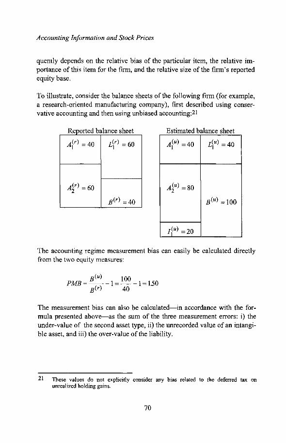
Accounting Information and Stock Prices
quently depends on the relative bias of the particular item, the relative importance of this item for the firm, and the relative size of the finn's reportedequity base.
To illustrate, consider the balance sheets of the following finn (for example,a research-oriented manufacturing company), first described using conservative accounting and then using unbiased accounting:21
Estimated balance sheet
AfU) =40 Liu) =40
Aiu) =80
B(u) =100
Ifu) =20
h tR rtdblepo e a ance s ee
Afr) =40 Lir) =60
Air) =60
B(r) =40
The accounting regime measurement bias can easily be calculated directlyfrom the two equity measures:
PMB =B(u) _ 1= 100 - 1=150B(r) 40
The measurement bias can also be calculated-in accordance with the formula presented above-as the sum of the three measurement errors: i) theunder-value of the second asset type, ii) the unrecorded value of an intangible asset, and iii) the over-value of the liability.
21 These values do not explicitly consider any bias related to the deferred tax onunrealized holding gains.
70

Research Design Considerations
(O.60.(~-1))+tWo-(O.60.(~-1))PMB = 40/ = 0.50 +0.50 + 0.50 =1.50
1100
The marginal PMB is in this case apparently 0.50" for each issue. Acalculation technique of this kind will subsequently be used in order toestimate firm or specific industry sector measurement biases. The effort willnecessarily be somewhat crude since a nun1ber of assumptions, for example,regarding the growth rate and the inflation rate have to be made. Also, theaverage economic lives and annual value change of different firms' assetsmust be estimated. Annual expenditures regarding R&D and future-orientedadvertising must be identified. The average investment-to-harvest timelagmust be estimated. The relative importance of different items for differentfirms must also be identified. Some of this information can be extractedfrom annual reports, but other details have to be approximated. In this study,only the factors that are expected to create the most significant biases willbe considered.
3.1.1.3 Calculation ofthe most significant measurement biases
As in Fruhan's US study from 1979, the main sources of large permanentbiases associated with the Swedish accounting regime can most likely betraced to the historical cost valuation of long lived assets and the expensingprocedure of investments in intangibles. The over-valuation of deferred taxliabilities can possibly also create non-trivial measurement biases forseveral firms. To illustrate the potential size of these biases, different tablesare calculated using the formulas presented above.
Tangible assetsJohansson and Ostman (1995) illustrated with an example that the conservative measurement bias22 will be permanent (in the relative sense of assumption A.3) if three (strict) conditions are fulfilled: 23
22 The current cost method developed by Edwards and Bell (1961) was used as a proxyfor 'ideal' measurement.
23 Additionally, an assumption of no technical development of the asset type is implicitlyassumed.
71

Accounting Information and Stock Prices
Hi) The units have uniform economic lives, uniform rates of depreciation, the same cost of acquisition in real terms and thesame number ofunits are replaced each year.ii) The historical rate of inflation has been constant since thefirst ofthe existing units was acquired.iii) The same rate ofinflation will continue. "
Johansson and Ostman (1995, p. 137)
These rather restrictive conditions may not be expected to hold for fimls ingeneral at a present date, but can still serve as a useful starting point for anestimation procedure of a permanent measurement bias. It can further beshown that their observation of a constant measurement bias also holdswhen allowing for constant annual growth in the number of units of theasset. The measurement bias, will ceteris paribus, always be snlaller whengrowth is positive, given a positive inflation rate. The constant measurementbias, given these particular conditions, can be described as follows in termsof equation [3: 1]:
[3:7] N ( ) (1:;r {l- ~)Asset bias = L (l+i)n -1 . N . (I-i)
n=O'----v----' ~ AP .(1-~) ~Inflation L.J ( )n N Component
Component n=O 1+q''-----...-----
Asset Weight
where
AP = the acquisition price of one unit of the asset in nominal termsn = the age of the asset (in years)N = the economic life of the asset typeq = the annual percentage growth in number of acquired unitsi = the annual unrecorded value change7:= the tax rate
To understand the relative importance of the components that generate ameasurement bias on a depreciable asset, consider figure 3.1a (10%inflation and no growth) and 3.1b (10% inflation and 10% growth). The
72

Research Design Considerations
calculations have been based on [3:7], and on the following specificassumptions:24
• One item of the asset is bought at the beginning of every year.• One sin1ilar old asset is simultaneously scrapped (salvage value = 0).• If growth occurs, more units (a fixed percentage) of the asset are bought
every year.• The units have uniform economic lives (10 years), uniform rates of de
preciation (straight line), and the same cost of acquisition in real terms.• The historical rate of inflation has been constant (10%) since the first of
the existing units was acquired. The same rate of inflation will continue.• The measurement bias is calculated at the end of the year.25
• The deferred tax on holding gains is not considered.
24
25
These conditions are largely borrowed from an example in Johansson and Ostman,1995 pp. 136. Their example was provided to illustrate that growth in equity will besimilar irrespective of traditional measurement principals or current cost measurementunder the specified conditions, i.e. the case of a permanent measurement bias.This means, in combination with beginning-of-the-year acquisitions, that if there is nogrowth, the company holds one unit of the asset that is one year old, one that is twoyears old, etc., and that the oldest unit held is 10 years old and fully depreciated. Thismeans that the nlean age of the units the company holds is 5.5 years.
73

Accounting Information and Stock Prices
1.6 0.06
1.40.05
en 1.2 en..0.04 :ac:
CD 1.0c: ..0 c:C- 0.8 0.03 ~E0 e(.) 0.6 ::sen 0.02 :IC'CS
iii CD0.4 :E
0.20.01
0.0 0.002 3 4 5 6 7 8 9 10
Age of asset in years
I [J Inflation component ~ Asset weight -&-Measurement bias)
Figure 3.la An illustration ofthe components that generate a measurement bias(before tax) on depreciable assets with a lO-year economic life given10% inflation and no growth.
1.6 0.06
1.40.05
en 1.2 en..0.04 :ac:
CD 1.0c ..0 c:c- 0.8 0.03 ~E0 e(.)
0.6 ::sen 0.02 :IC'CS
iii CD0.4 :E
0.20.01
0.0 0.002 3 4 5 6 7 8 9 10
Age of asset in years
CD Inflation component ~ Asset weight -&-Measurement bias I
Figure 3.1b An illustration ofthe components that generate a measurement bias(before tax) on depreciable assets with a lO-year economic life given10% inflation and 10% annual growth.
74

Research Design Considerations
The inflation component is identical in the two figures. It is obviously apositive function of the holding period of the asset (its age). The assetweight, on the other hand, is a decreasing function of the age of the asset,mainly due to the depreciation scheme, but also due to the lower earlier acquisition price of each unit of the asset in nonlinal terms (due to inflation).These two off-setting factors are combined into a measurenlent bias fromeach year's investment. The measurement bias for each year is illustrated inthe figures as a dot (joined by a line). Each dot illustrates the contribution tothe total measurement bias (the right hand y-scale is used) of the asset of aparticular age. The total measurement bias (before tax) constitutes the sumof the measurement biases of each year's investment. The totalnleasurement bias, add up the values represented by the dots in the figures,equals 0.39 and 0.34. Given positive growth, the weights are relativelylarger for the newer assets, and therefore the bias is reduced.
An important insight gained fronl these figures is that the relative contribution to the total measurement bias of a depreciable asset first increases withage, reaches a maximum, and then decreases with age. The measurementbias of a firm holding an unbalanced portfolio of the asset type will thusvary considerably over time. A portfolio of relatively newer assets (e.g. thegrowth case above) will have a smaller measurement bias compared with acompletely balanced portfolio.
The illustrations above have been restricted to one level of inflation rate(10%) and an asset type with one particular economic life (10 years). Table3.1 illustrates the measurement bias according to [3 :7] (excluding the deferred tax effect), for different combinations of inflation rate and economiclives of a depreciable asset, given 5% constant annual growth, and the previously listed assumptions.26
26 Appendix A contains similar tables showing both 0% and 10% growth.
75
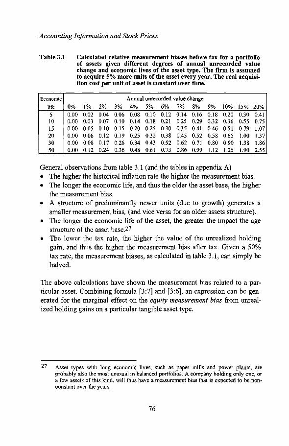
Accounting Information and Stock Prices
Table 3.1 Calculated relative measurement biases before tax for a portfolioof assets given different degrees of annual unrecorded valuechange and economic lives of the asset type. The firm is assumedto acquire 5% more units of the asset every year. The real acquisition cost per unit of asset is constant over time.
Economic Annual unrecorded value change
life 0% 1% 2% 3% 4% 5% 6% 7% 8% 9% 10% 15% 20%
5 0.00 0.02 0.04 0.06 0.08 0.10 0.12 0.14 0.16 0.18 0.20 0.30 0.4110 0.00 0.03 0.07 0.10 0.14 0.18 0.21 0.25 0.29 0.32 0.36 0.55 0.7515 0.00 0.05 0.10 0.15 0.20 0.25 0.30 0.35 0.41 0.46 0.51 0.79 1.0720 0.00 0.06 0.12 0.19 0.25 0.32 0.38 0.45 0.52 0.58 0.65 1.00 1.3730 0.00 0.08 0.17 0.26 0.34 0.43 0.52 0.62 0.71 0.80 0.90 1.38 1.8650 0.00 0.12 0.24 0.36 0.48 0.61 0.73 0.86 0.99 1.12 1.25 1.90 2.55
General observations from table 3.1 (and the tables in appendix A)• The higher the historical inflation rate the higher the measurement bias.• The longer the economic life, and thus the older the asset base, the higher
the measurement bias.• A structure of predominantly newer units (due to growth) generates a
snlaller measurement bias, (and vice versa for an older assets structure).• The longer the economic life of the asset, the greater the impact the age
structure of the asset base.27
• The lower the tax rate, the higher the value of the unrealized holdinggain, and thus the higher the measurement bias after tax. Given a 50%tax rate, the measurement biases, as calculated in table 3.1, can simply behalved.
The above calculations have shown the measurement bias related to a particular asset. Combining formula [3:7] and [3:6], an expression can be generated for the marginal effect on the equity measurement bias from unrealized holding gains on a particular tangible asset type.
27 Asset types with long economic lives, such as paper mills and power plants, areprobably also the most unusual in balanced portfolios. A company holding only one, ora few assets of this kind, will thus have a measurement bias that is expected to be nonconstant over the years.
76

[3:8]
Research Design Considerations
A(r)_k_. Bias T.A.
PMB T.A. = TA(r) kk B(r) /
/ TA(r)
where
PMB[·A. = the marginal PMB ofa tangible assets of type k
A(r)_k_ = the relative importance of the asset type (k)TA(r)
B(r) =the ratio ofbook value of equity to total assets (solidity)TA(r)
BiasI·A. = the measurement bias after tax of asset type k
The marginal measurement bias of an asset type can thus simply be generated by multiplying the measurement bias by the relative importance of theasset type for the firm, and dividing the product by the firm's solidity. Table3.2 illustrates the effect of this additional factor-relative importance divided by solidity-for some possible combinations.
Table 3.2 The relative importance of an asset type (as a percentage of totalassets) divided by different possible solidity levels.
Relative Solidity (equity-to-assets ratio)importance 10% 20% 30% 40% 50% 60% 70% 80% 90% 100%
0% 0.0 0.0 0.0 0.0 0.0 0.0 0.0 0.0 0.0 0.010% 1.0 0.5 0.3 0.3 0.2 0.2 0.1 0.1 0.1 0.120% 2.0 1.0 0.7 0.5 0.4 0.3 0.3 0.3 0.2 0.230% 3.0 1.5 1.0 0.8 0.6 0.5 0.4 0.4 0.3 0.340% 4.0 2.0 1.3 1.0 0.8 0.7 0.6 0.5 0.4 0.450% 5.0 2.5 1.7 1.3 1.0 0.8 0.7 0.6 0.6 0.560% 6.0 3.0 2.0 1.5 1.2 1.0 0.9 0.8 0.7 0.670% 7.0 3.5 2.3 1.8 1.4 1.2 1.0 0.9 0.8 0.780% 8.0 4.0 2.7 2.0 1.6 1.3 1.1 1.0 0.9 0.890% 9.0 4.5 3.0 2.3 1.8 1.5 1.3 1.1 1.0 0.9
100% 10.0 5.0 3.3 2.5 2.0 1.7 1.4 1.3 1.1 1.0
77
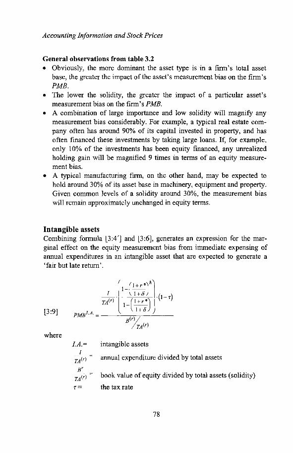
Accounting Information and Stock Prices
General observations from table 3.2• Obviously, the more dominant the asset type is in a firm's total asset
base, the greater the in1pact of the asset's measurement bias on the firm'sPMB.
• The lower the solidity, the greater the inlpact of a particular asset'smeasurement bias on the firm's PMB.
• A combination of large importance and low solidity will magnify anymeasurement bias considerably. For example, a typical real estate con1pany often has around 90% of its capital invested in property, and hasoften financed these investments by taking large loans. If, for example,only 10% of the investments has been equity financed, any unrealizedholding gain will be magnified 9 times in terms of an equity measurement bias.
• A typical manufacturing fim1, on the other hand, may be expected tohold around 30% of its asset base in machinery, equipment and property.Given common levels of a solidity around 30%, the measurement biaswill remain approximately unchanged in equity terms.
Intangible assetsCombining formula [3:4'] and [3:6], generates an expression for the marginal effect on the equity measurement bias from immediate expensing ofannual expenditures in an intangible asset that are expected to generate a'fair but late return'.
ITA(r) .
[3:9]
where
l-(\:r;f ( )-1---:"(-1+-r*~) .1- T
1+8PMB1.A. =-----------:---
B(r)// TA(r)
LA.= intangible assetsI
TA(r) annual expenditure divided by total assets
Br
TA(r) book value of equity divided by total assets (solidity)
,= the tax rate
78
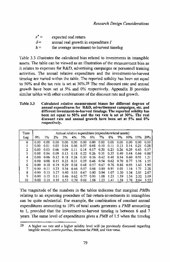
Research Design Considerations
r*= expected real return8 = annual real growth in expenditure Ih = the average investment-to-harvest timelag
Table 3.3 illustrates the calculated bias related to investments in intangibleassets. The table can be viewed as an illustration of the measurement bias asit relates to expenses for R&D, advertising campaigns or personnel trainingactivities. The annual relative expenditure and the investment-to-harvesttimelag are varied within the table. The reported solidity has been set equalto 50% and the tax rate is set at 30%.28 The real discount rate and annualgrowth have been set at 5% and 0% respectively. Appendix B providessimilar tables with other combinations of the discount rate and growth.
Table 3.3 Calculated relative measurement biases for different degrees ofannual expenditures for R&D, advertisement campaigns, etc. anddifferent investment-to-harvest tinlelags. The reported solidity hasbeen set equal to 50°A. and the tax rate is set at 30%. The realdiscount rate and annual growth have been set at 5% and O°A.respectively.
Time Annual relative expenditure (expenditure/total assets)Lag 0% 1% 2% 3% 4% 5% 6% 7% 8% 9% 10% 15% 20%
0 0.00 0.00 0.00 0.00 0.00 0.00 0.00 0.00 0.00 0.00 0.00 0.00 0.001 0.00 0.01 0.03 0.04 0.06 0.07 0.08 0.10 0.11 0.13 0.14 0.21 0.282 0.00 0.03 0.06 0.09 0.11 0.14 0.17 0.20 0.23 0.26 0.29 0.43 0.573 0.00 0.04 0.09 0.13 0.18 0.22 0.26 0.31 0.35 0.40 0.44 0.66 0.884 0.00 0.06 0.12 0.18 0.24 0.30 0.36 0.42 0.48 0.54 0.60 0.91 1.215 0.00 0.08 0.15 0.23 0.31 0.39 0.46 0.54 0.62 0.70 0.77 1.16 1.556 0.00 0.10 0.19 0.29 0.38 0.48 0.57 0.67 0.76 0.86 0.95 1.43 1.907 0.00 0.11 0.23 0.34 0.46 0.57 0.68 0.80 0.91 1.03 1.14 1.71 2.288 0.00 0.13 0.27 0.40 0.53 0.67 0.80 0.94 1.07 1.20 1.34 2.01 2.679 0.00 0.15 0.31 0.46 0.62 0.77 0.93 1.08 1.23 1.39 1.54 2.32 3.09
10 0.00 0.18 0.35 0.53 0.70 0.88 1.06 1.23 1.41 1.58 1.76 2.64 3.52
The magnitude of the numbers in the tables indicates that marginal PMBsrelating to an expensing procedure of fair-return-investments in intangiblescan be quite substantial. For example, the combination of constant annualexpenditures amounting to 10% of total assets generates a PMB amountingto 1, provided that the investment-to-harvest timelag is between 6 and 7years. The same level of expenditures gives a PMB of 1.5 when the timelag
28 A higher tax rate and a higher solidity level will (as previously discussed regardingtangible assets), ceteris paribus, decrease the PMB, and vice versa.
79

Accounting Information and Stock Prices
approaches 10 years. Provided that, perhaps more realistically, the realamount spent every year has steadily increased (by 10%), the PMB forsimilar investment-to-harvest timelags will amount to 0.80 and 1.15 respectively.29 How large estimated measurement bias does this zero-coupon-bondapproach generate compared with an assumption of a conventional lineardepreciation scheme? Appendix C shows a table that illustrates the necessary economic life of an intangible asset, depreciated linearly, in order togenerate equivalent PMBs as calculated by the zero-coupon bond approach.The table shows, for example, that an investment-to-harvest timelag of 5years generates approximately the same PMB as a 10 to 11 year economiclife assunling linear depreciation.
It is well known that the tinlelag between the early research phase and thelaunching of a product in the pharmaceutical industry is generally very long(10 to 20 years). It is also well known that the annual expenditures on R&Din the pharmaceutical industry are significant.30 The expected investmentto-harvest timelag of an advertising campaign cannot be expected to be aslong as that of R&D efforts. The annual expenditures in, for example,brandname-intensive consumer goods industries can, however, besubstantia1.31 For example, a two-year timelag and 15% annual expendituresgenerate a marginal PMB amounting to 0.43 according to table 3.3. Theinvestment-to-harvest tinlelag for personnel training activities is, to myknowledge, almost unexplored. Documented knowledge of annualexpenditures on such activities is also quite limited.32
29
30
31
32
See appendix B. The tables also indicate that a higher real discount rate (e.g., takinglarge expected risk into account), somewhat increases the PMBs, especially for thelonger investment-to-harvest timelags, but has only a nlarginal effect on the PMB for ashorter timelag.Astra, a Swedish pharmaceutical firm, has annually expensed R&D efforts amountingto between lO-15°A, of total assets betwee~ the years 1966 and 1994 (see Astra's annualreports).Swedish firms have in general not disclosed their annual marketing expenditures.International examples of marketing expenditures have been identified for Heineken,the Dutch Brewery, and Coc~ Cola, the US soft dlink company, from the Extelcompany research database for 1993 and 1994. Heineken spent on average 14% andCoca Cola 10% in relation to total reported assets. Annual marketing and advertisementexpenditures for a brandname-intensive firm can apparently amount to 10% of reportedassets or more.Swedish firms rarely disclose information concerning their annual expenditures onpersonnel training activities. Angpanneforeningen, a Swedish consulting firm, is anexception. Angpanneforeningen's average annual personnel training expenses
80
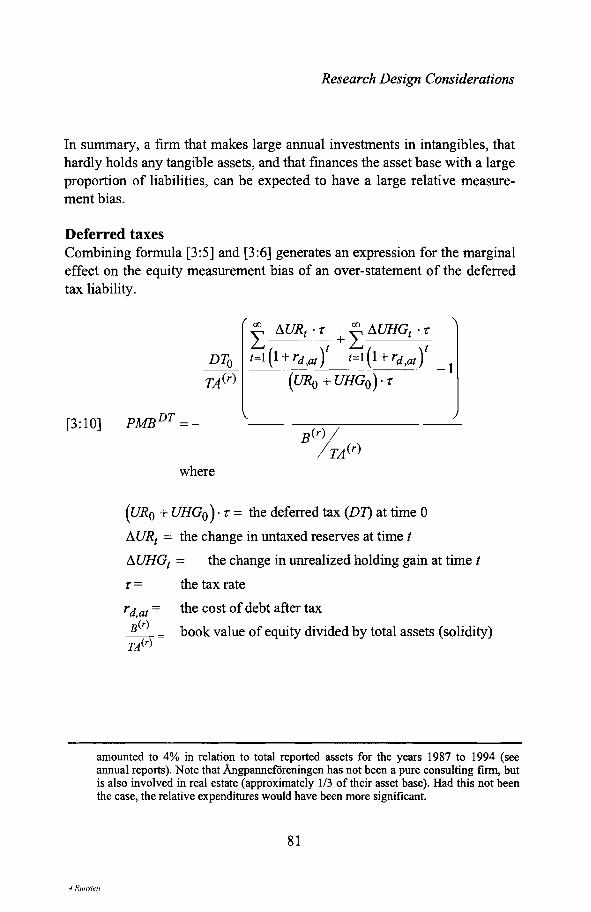
Research Design Considerations
In summary, a firm that makes large annual investments in intangibles, thathardly holds any tangible assets, and that finances the asset base with a largeproportion of liabilities, can be expected to have a large relative measuren1ent bias.
Deferred taxesCombining fom1ula [3:5] and [3:6] generates an expression for the marginaleffect on the equity measurement bias of an over-statenlent of the deferredtax liability.
DTO
TA(r)
f I1.URt ., +f I1.UHGt .,
t=l(l+rd,atr t=l(l + rd,at}t----~------- -1
(URO + UHGO)·"
[3:10] PMB DT =--------------B(r) I
ITA(r)
where
(URO + UHGO) . ,,= the deferred tax (D1) at time 0
~URt = the change in untaxed reserves at time t
~UHGt = the change in unrealized holding gain at time t
" = the tax rate
Yd,at =B(r)
TA(r)
the cost of debt after tax
book value of equity divided by total assets (solidity)
amounted to 4% in relation to total reported assets for the years 1987 to 1994 (seeannual reports). Note that Angpanneforeningen has not been a pure consulting firm, butis also involved in real estate (approximately 1/3 of their asset base). Had this not beenthe case, the relative expenditures would have been more significant.
81
.j Runsten

Accounting Information and Stock Prices
Assuming that all the deferred taxes should be repaid at a single point intime, the equation can be simplified.33
[3: 11]DTO [ 1 IJ
TA(r) (1 + r )PPMB DT =_ d,at
B(r) IITA(r)
where
p = the average length of time until the tax liabilities areexpected to be paid
Table 3.4 illustrates the calculated bias related to the over-valuation tendency of deferred taxes using equation [3: 11]. The relative size of the deferred tax liability and the length of time until expected payment are variedin the table. The solidity is set at 30%, and an after-tax cost of debtamounting to 7% (consistent with, for example, 30% tax rate and 10% costof debt) is used.34
33
34
This simplification can be viewed as an approximation to identifying the weightedaverage time period left until repayment of the liability.A higher discount rate would generate a larger bias and vice versa.
82

Research Design Considerations
Table 3.4 Relative measurement bias for different sizes of the deferred taxliability and different time lengths until payment. The reportedsolidity is set at 30% and 70/0 is used as the after-tax cost of debt.
Time Deferred tax liability/Total assets (%)Lag 0% 5% 10% 15% 20% 25% 30% 35% 40% 45% 50% 55% 60%
0 0.00 0.00 0.00 0.00 0.00 0.00 0.00 0.00 0.00 0.00 0.00 0.00 0.001 0.00 0.01 0.02 0.03 0.04 0.05 0.07 0.08 0.09 0.10 0.11 0.12 0.132 0.00 0.02 0.04 0.06 0.08 0.11 0.13 0.15 0.17 0.19 0.21 0.23 0.253 0.00 0.03 0.06 0.09 0.12 0.15 0.18 0.21 0.24 0.28 0.31 0.34 0.374 0.00 0.04 0.08 0.12 0.16 0.20 0.24 0.28 0.32 0.36 0.40 0.43 0.475 0.00 0.05 0.10 0.14 0.19 0.24 0.29 0.33 0.38 0.43 0.48 0.53 0.576 0.00 0.06 0.11 0.17 0.22 0.28 0.33 0.39 0.44 0.50 0.56 0.61 0.677 0.00 0.06 0.13 0.19 0.25 0.31 0.38 0.44 0.50 0.57 0.63 0.69 0.758 0.00 0.07 0.14 0.21 0.28 0.35 0.42 0.49 0.56 0.63 0.70 0.77 0.849 0.00 0.08 0.15 0.23 0.30 0.38 0.46 0.53 0.61 0.68 0.76 0.84 0.91
10 0.00 0.08 0.16 0.25 0.33 0.41 0.49 0.57 0.66 0.74 0.82 0.90 0.98~00 0.00 0.17 0.33 0.50 0.67 0.83 1.00 1.17 1.33 1.50 1.67 1.83 2.00
It is evident from table 3.4 that orlly a large deferred tax liability with afairly long life expectancy generates a measurement bias that exceeds 0.5.Note that a deferred tax, related to untaxed reserves, in excess of 20-30% ofreported assets, is an unlikely state.35 The deferred tax related to a largeunrealized holding gain (as discussed in the previous sections), can, however, be potentially fairly large. If the time to realization, and thus the timeto payment of the tax liability is expected to be long, the relative overvaluation of the liability may be significant. In the extreme case when thetimelag to repayment approaches infinity, the liability approaches zero andthe n1easurement bias equals DTIB.
35 If the solidity amounts to 30%, as assumed in the table, the maximum deferred tax(related to untaxed reserves) is equal to
30% . r which, with a tax rate amounting to e.g. 50%, gives a maximum DT/A =
(1- r)30%.
83

Accounting Information and Stock Prices
3.1.1.4 The measurement bias as calculated by Fruhan
Fruhan (1979) made calculations of book value of owners' equity adjustedfor capitalized investn1ents in advertising and R&D, and with assets revalued to estimated replacement costs. His sample included 72 US firms at theend of 1976. He deliberately selected firms that consistently, over a ten-yearperiod, had generated a high ROE (exceeding the cost of equity capital). Theselection procedure generated a sample of firms that were extreme performers and/or for which the conservative accounting procedure tended to understate the book value of equity (and thus overstate ROE). Fruhan acknowledged the difficulty regarding the assessment of a reasonable life expectancy and amortizing schedule for R&D and advertising expenditures. Referring to previous studies, he assumed that an advertising expenditure hadan economic life of six years and that its amortization would follow thedouble declining balance n1ethod. He further assumed that R&D expenditures had a ten-year life and straight line depreciation. Some 50% of thefirms in his sample had disclosed domestic inventory and net plant andequipment at replacement cost.36 Extracting data from tables 1-9 and 1-11in Fruhan (ibid.), the following table has been generated. The data havebeen summarized for five different industry sectors.37
36 Note that the replacement cost of land and foreign assets is not adjusted for.37 Specification of firms in each industry sector:
Pharmaceutical Consumer Retail Specialized ManufacturingGoods Service
American Home pro Avon Products Caldor, Inc. Dow Jones Champion Spark PlugBristol-Myers Chesebrough-Ponds Dillon Cos. Dun & Bradstreet Eastman KodakEli Lilly Coca-cola Eckerd (Jack) Emery Air freight Emerson ElectricMarion Labs Dr. Pepper Loehmann's H&RBlock IBMMerck Gillette Longs Drug Stores Marsh & McLennan LubrizolRobins, A.H. Heublein Lucky Stores McDonalds Nalco ChemicalRorer-Amchen Kellogg Melville Corp. Merchants, Inc. National ChemsearchScherling-Plough PepCom Industries New Process Co. Prentice-Hall, Inc. PurolatorSearle, G.D. PepsiCo Inc. Rockower Bros. Roadway Express Square DSmithkline Corp. Procter & Gamble Weis-Market Rollins, Inc. Thomas & Betts Corp.Sterling Drug Revlon Winn-Dixie Stone & Webster XeroxTampax Reynolds,RJ. Wackenhut
Russell Stover Yellow Freight Syst.Candies
84

Table 3.5
Research Design Considerations
Calculated accounting measurement bias for five subgroups offirms extracted from tables 1-9 and 1-11 in Fruhan (1979).
(1) (2) (3) (4) (5)Industry sector Number of Estimated Estimated Estimated Market-to-
firms used advertising replacement total bookin each and R&D cost premium premium premiumestimate premium(2)/(3) (avera~e) (average) (average) (average)
Pharmaceutical 12/9 0.28 0.25 0.57 1.93Consumer Goods 13/8 0.16 0.30 0.46 1.94
Retail 11/2 0.04 0.18 0.21 1.38Specialized Service 12/4 0.04 0.12 0.15 2.29Manufacturing 11/8 0.11 0.39 0.51 1.77
The first column indicates how nlany firm observations the premium averages rely on. The replacement cost adjustment has only been performed onsome of the firms. The second column includes the average estimated premium related to the capitalization of advertising and R&D expenditure. Ithas been calculated as the unweighted average of firm specific adjusted equity divided by reported equity minus one. The third column includes theaverage estimated premiunl related to replacement cost valuation. It has alsobeen calculated as adjusted equity divided by reported equity minus one.The fourth column includes the average total premium, and the fifth columnincludes the average market-to-book value premium for the same firms calculated at the end of 1976.38 It is calculated as the market value of equity atthe end of December 1976 divided by reported equity minus one.
Next follows a discussion of these calculated biases in the light of the'measurement bias tables' presented in the previous section. It should bekept in mind that the data are US, and cover a small group of well performing firms at a single point in tinle. The marginal tax rate was approximately
38 Studying the last column of table 3.5, one may note that Fruhan's adjustment procedureexplains between 7% to 30% of the actual market-to-book value premium. This meansthat expected positive abnormal earnings are expected to explain the remaining 93% to70%. This may well be reasonable given that the best performing firms available wereincluded in Fruhan's study. The utilized measurement bias estimation scheme may,however, also have been too conservative.
85

Accounting Information and Stock Prices
50% at this time39 and the average annual inflation rate40 had been 7.2%and 5.9% during the five and ten years respectively, preceding 1976.
Estimated measurement biases related to intangibles-to be compared with table 3.3
• The R&D intensive group of pharmaceuticals had on average a bias of0.28 caused by the capitalization of R&D and advertising expenditure. Asimilar measurement bias is consistent with, for example, a four-yearinvestment-to-harvest timelag and annual R&D expenditures amountingto 5% in relation to total assets (given the solidity and tax assumptions oftable 3.3).
• The brandname-intensive firms41 in the consumer goods sector had anaverage measurement bias caused by the capitalization of intangible assets of 0.16. In terms of table 3.3, this measurement bias is equivalent toannual expenditures of 5% relative to the asset base of the firm and toslightly more than a two-year investment-to-harvest timelag.
• The manufacturing sector included 'high-tech' firms such as ffiM, Xeroxand Eastman Kodak, which can be expected to have 'invested' heavily inboth R&D and marketing. The average estimated bias was still as low as0.11 for this group. The relative bias effect of intangibles has presumablybeen reduced by the fact that these firms also held a large share of tangible assets. The relative measurement bias may have been reduced furtherby a particularly high solidity in this group of firms.
• With regard to the other sectors, the R&D and advertising capitalizationscheme identified very small measurement biases. Note that Fruhan'sadjustment scheme did not identify biases due to expenses for personneltraining activities. Capitalization of such expenses would probably havethe most in1portant effect on the measurement bias of the firms in thespecialized service sector.
39 Fruhan (1979)40 See Consumer Price Index, Exhibit 17 in Ibbotson and Sinquefield (1989).41 This group includes firms such as Coca-Cola, PepsiCo, Kellogg and Procter & Gamble.
86

Research Design Considerations
Estimated measurement biases caused by replacement cost valuation of inventory and plant and equipment-to be compared withtables 3.1 and 3.2
• The estimated measurement bias caused by replacement cost valuationvaried between 0.12 and 0.39. The highest average bias was shown forthe firms classified as manufacturing firms. This is not surprising asthese firms can be expected to have held a significant share of their assets as plant and equipment and have held a large inventory (possiblyvalued according to the LIFO method). The service sector had the smallest identified replacement cost bias. This is also in line with expectationsas firms in this sector generally hold no inventory and often need a verysnlall base ofM&E.
• Fruhan's sample of firms did not include any firms with tangible assetswith very long economic life (e.g. real estate firms). Such a group offirms would have been expected to have a large premium arising fromthe replacement cost adjustment.
87

Accounting Information and Stock Prices
3.1.2 Expected growth persistence factor (GPF)
One of the slope coefficients in several of the proposed regression specifications in Chapter 2 is assumed to be a function of the expected ability of afiml to persistel1tly generate abnormal perfomlance. Such ability is expectedto differ among different types of firms. The level of the GPF is mainlyexpected to be a function of the firm's growth potential and the degree ofindustry competitiveness. A thorough analysis of the competitive characteristics of an industry, and their implications for an individual company'sgrowth potential and expected success in defending competitive advantages,is obviously a major undertaking.42 In order to control for the most extremecases of heterogeneity in this respect, a simple classification scheme will,however, have to suffice in this study. The scheme used is based on published accounting data and the presumption that high GPF firms should becharacterized by having experienced strong growth and a stable positiveresidual return.
3.1.3 Expected validity of historical ROE
Market-based accounting research has commonly relied on recently published earnings (or ROE) as the base for expected performance for futureperiods. The validity of relying on such a simple prediction procedure, however, is expected to be different for different types of business activities.The validity of s110rt-term historical ROE performance as an indicator offuture performance is expected to be particularly poor if the firm's businessis characterized either by a long production cycle (several years) with revenue recognition at completion, or the realization of holding gains being themain source of profit generation.43 The first is typical of the building andconstruction industry, and the latter is typical of real estate and investmentcompanies. The expected short-term ROE validity problem stems from thefact that the recognition of profits in these industries tends to be particularlynon-continuous and the timing can be particularly affected by managementdiscretion.
42
43
Such an analysis is presumably important for an investor considering which shares tobuy on the stock market.High and/or fluctuating inflation rates are expected to magnify these problems.
88

Research Design Considerations
3.1.4 Summarized description of firm characteristicsTable 3.6 provides a summary of different aspects related to the three firmcharacteristics discussed in this chapter. The first column contains the threefirm characteristics with further subgroups. The second column indicates themain factors that are thought to signify the importance and size of the characteristic. The third column gives examples of typical industries that areprone to be extreme in each dimension. The fourth column indicates how afirm characteristic can be identified and/or quantified. The final columnprovides examples of how a certain fiml characteristic is expected to influence the regression coefficients in the proposed regression specifications ofChapter 2.
For a group of firms with a small expected persistent measurement bias,with similar general business conditions and with a current ROE that is informative, the simple valuation regression model M.l can be expected, ifever, to perform well. A weaker and more unstable regre'ssion result can beexpected, with a more heterogeneous sample of firms (in these dimensions).Given a reasonable quantification of the PMB and given that current ROE isinformative, the valuation regression model M.2 is expected to perform better than M.l with a heterogeneous sample of fimls. In the value change regression specifications, M.3 and M.4, a sample including firms with largeexpected permanent n1easurement biases is expected to generate a slopecoefficient, related to change in equity ( el ), that exceeds one.
89

Table 3.6 Summary table of identified firm characteristics, the main factors signifying the characteristic, typicalfirms, some identification and quantification issues, and examples of expected effects on model coefficients.
Characteristic Main Factors of Influence Typical firms How identify? Affected modelHow quantify? coefficient
1. Persistent measurement bias PMB=I=O
• Intangible assetsR&D Pharmaceutical Capitalized R&D
• Relative importance High-tech expensesMarketing intensive • Timelag from cash out to Consumer products Capitalized advertising(brandname) cash in expensesStructure/personnel • Growth Consulting Capitalized personnel PMB> 0
training expenses a > 0 inM.l
• Assets with long economic life • Relative importance Real estate el > 1 in M.3-4• Age of assets Investment firms• Relevance of depreciation Power plant Estimate
pattern Paper mill current cost• Growth Shipping• Inflation rate
• Deferred taxes • Relative importance Estimate• Time to payment current liability• Cost of debt
2. Firm experiencing abnormal • Industry growth Growth> x G, A, & Tgrowth and/or abnormal return • Barriers to entry & ROE>p A (GPF)persistence • Substitutes A & e2 are
• Price elasticity ROEt is extreme extreme orunstable
3. Current ROE is likely to be a E[RR] =?poor indicator of performance
• Short-term ROE is easily • Revenue recognition criteria Construction company Industry sector A& e are'manipulated' by management • Realization ofholding gains Holding activity unstaf,le
R2 is low

Research Design Considerations
3.2 Changes in the economic climateSome regressions in this study will be run repeatedly using yearly data formore than 25 different years. Other regressions will be run for windows aswide as up to ten years. It is obvious that the association between accounting information and the level or change in stock prices over such longperiods of time may be influenced by a large array of changes in theeconomic climate, and changes in the institutional environment. Changes inthe econon1ic climate, in a broad sense, include issues such as generaleconomic growth, inflation rates, foreign exchange rates, as well as issuessuch as trade agreements with other countries, company and accountinglaws, and tax regulations. A continuously increasing number of actors on thestock market, for example, analysts, intermediaries, institutional and foreigninvestors constitutes another type of change over time. It is beyond thescope of this study to analyze the effects of all these factors on the actual regression results.
Two particular issues relating to the economic climate, however, areconsidered both possible and interesting to control for. These two issues arethe level and the pattern of the inflation rate, and the observable fluctuationsin the business cycle. The accounting description ofa firm's value and valuecreation given an accounting regime based on historical cost valuation is affected by the level of the inflation rate over many years. To what extent thedescription is affected depends largely on the kind of assets the particularfirm owns. Johansson and Ostman (1995, p. 143) give examples of industrysectors that can be expected to be more or less affected by high and/orchanging inflation rates. The most affected industry sectors are those inwhich firms hold a large number of assets with long economic life. If firmsof this type also have an unstable age structure of plant and equipment, andthe rate of inflation is high and fluctuating, the usefulness of the accountingdescriptions as indicators of firm performance is expected to be very limited. To empirically test this proposition, the regression specifications willbe run separately for different firm types at different points in time (or fordifferent time periods). Time periods will be chosen considering the actualinflation rate pattern.
91

Accounting Information and Stock Prices
If investors tend to have different expectations (e.g. optimistic versus pessimistic expectations) about the future performance of firms at differentstages in tl1e business cycle, this factor could generate unstable regressioncoefficients in the level regressions, and should preferably be controlled forin the long window regressions of M.3 to M.5.
3.3 Accounting changesBoth the firm characteristics and the changes in the economical climate discussed above relate to accounting issues. The focus is on the expected ability, or lack of ability, of the accounting convention to capture value andvalue creation for different types of firms under different environmentalconditions. These issues are related to the inherent difficulty for the outcome of an accounting procedure to explain value and value creation.Alongside these issues, changes in the accounting practice can be observed.The changing accounting practice may be seen as a response to a large arrayof factors. One such factor is a general trend towards international harmonization. The information demand of an increasing number of professionalinvestors is another obvious force. Other examples of factors that may trigger changes in the accounting regime are the emergence of, new types ofbusiness activities, new financial instruments, new taxation regulations,higher inflation rate levels, and fluctuating exchange rates.
In this study, the association between certain accounting numbers and thestock market price, or the price change, will be assessed. The two key accounting variables are the book value of owners' equity and accountingearnings. These measures are further combined, generating return on equityand growth in equity. ROE will also be compared to an estimated cost ofequity generating residual return estimates.
It is obvious from valuation equation [2: 16] that value (V) is a positivefunction of both book value of equity (B) and expected return on equity(ROE).44 As a simple guide to understanding (and classify) the effects ofdifferent measurement issues in tem1S of the chosen valuation model, consider figure 3.2.
44 In [2:32] V is also a positive function of a permanent measurement bias (PMB).
92

Research Design Considerations
B
... ..... .. .... ....... ...... .....
.' ....
'" III... .........
.... I
""". ....... ..... ......II • _ • .. . .. . . -.. . .. .. -.
"""",,"""
~
"
",
,,
,,,
,,,,
""..... -.. -. - - . - . -",. - .........IV' .....
B*•.I
I,-I-----I-----tr-.----t----t---t----t----+---IROE
........... ROE* ••••~
Figure 3.2 A simple illustration of the trade-off between book value of equityand ROE that generate economic value.
Assume that given B* and ROE*, the value of a firm is V*. Consider next analternative accounting convention generating different levels of B and ROE.Two main situations emerge:
I Higher book value of equity, lower ROE and V* is unchanged.II Lower book value of equity, higher ROE and v* is unchanged.
Most accounting measurement choices should be possible to classify in oneof the two 'trade-off categories (I & II), where, for example, an increasedbook value only comes at the expense of a lower ROE, and vice versa. Forinstance, a more conservative accounting convention will be expected togenerate lower book value of equity in con1bination with higher expectedROE. Given comprehensive accounting, the two conventions will eventuallyhave accounted for the same value creation and should thus also be valuedsimilarly.45 The management of many companies and the financial press,
45 This does not include effects related to the post-contracting role of accounting, such astaxation etc..
93

Accounting Information and Stock Prices
however, often seem to be very concerned about different accounting principles' effects on key financial ratios. Accounting for acquired goodwill,and its effect on earnings per share, return on equity and solidity is a typicalexample.
In the short-term (for one or a few years), a certain accounting measurementprinciple may simultaneously lead to both higher (or lower) book value ofequity and ROE. Situations III and IV should still not occur--economicvalue (V*) should remain unchanged, and provided that the nlarket isefficient, the market price should also remain the same. However, it isnaturally quite difficult in all situations to disentangle the effects of achosen accounting method for the current year and for a long series ofcoming years. Given such problems, situations III or IV may at least for a'shortsighted' observer seem to be the 'real' situation.
3.3.1 Accounting changes in Sweden 1965 - 1995Accounting changes can be classified as being related to either disclosure ofnew information or changes of measurement principles.
Accounting changes can be manifested in new regulations (laws), new recommendations and a new practice. Table 3.7a is based on (and indicates theapproximate date of) the initial formal issue of a new recommendation(regulation) regarding accounting disclosure issues during the period 1965 1995. Table 3.7b provides a similar overview of changing accounting methods.
94

Table 3.7a A summary of event dates since the mid 1960s of when a new type of accounting disclosure first was formally recommended by a standard setting body or formally required by a new law.Sources: FAR (1965 to 1995) and NBK's published recommendations.
More Information 1965 1970 1975 1980 1985 1990
# Consolidated statements
# Open disclosure ofinventory reserve FAR # 2-66
outline FAR 71 ABL (75)
ABL (75)
# Open disclosure of depreciationaccording to plan NBK (68) FAR # 1-69
# Current cost accounting
draft FAR 81, FAR # 3-83
outline FAR 80
# Interim reports
# Disclosure of effects due tochanged accounting principles
# Disclosure ofR&D expenses
NBK (68) ABL (75)
ABL (75) RR# 5-94
BFN R 1-88
Abbreviation listABL Companies Act (law)BFL Accounting Act (law)FAR Swedish Institute of Authorized Public Accountants (recommending body)BFN Accounting Board (recommending body)RR The Swedish Financial Accounting Standards Council (recommending body)NBK Industry and Commerce Stock Exchange Committee

Table 3.7b A summary of event dates since the mid 1960s of when a new type of accounting method first was formallyrecommended by a standard setting body or formally required by a new law.Sources: FAR (1965 to 1995) and NBK's published recommendations.
draft FAR 76 FAR # 11-78 RR # 1-91triggered by Balans (Dec. 87)
BFL (75) out. FAR 83 draft FAR 86 FAR #13-88 RR # 4-93
New Accounting Method
# Consolidation method- Par value method (~Poolingmethod)- Purchase method
# Accounting for goodwill- Depreciation (maximum life)- Write-off against equity
# Extraordinary items
1970
outline FAR 71
outline FAR 71
1975 1980
draft FAR 76 FAR # 11-78
1985 1990
RR# 1-91
statement #12 FARs Accounting Committee (86)RR# 6-95
outline FAR 80found not compatible with BFL (75)
FAR # 4-66
BFN # 7-90
draft RR 95
if integratedif independent
outline FAR 87
outline FAR (85)
FAR # 4-82
draft FAR 81
draft FAR 76
# Accounting for associated companies- Cost method- Information about retained share in profit- Equity method
# Leasing- Delayed holding gain realization of
a sale & lease back transaction- Substance over form accounting of
a sale & lease back transaction- Capitalization of fmancialleases
# Accounting for pension cost and liability
# Receivables and liabilities in foreign currency- Closing day currency rate
# Translation of foreign subsidiaries- Monetary/non-monetary method (temporal method)- All current method

Research Design Considerations
It is important to note that accounting practice in many cases tends to precede formal regulation. As an instructive example, Hanner (1980) discussesthe effect of the Companies Act (ABL 1975) and the Accounting Act (BFL1976):
tI••••• introduced many changes regarding the annual report. Newrequirements included: complete and public consolidated statements, for larger companies open disclosure of hidden reservesrelated to inventory valuation, cash-flow statements and interimreports. These new legal requirements, however, merely reflectedthe development that had already taken place in practice duringthe 10 - 20 years preceding 1975."
Hanner (1980)46
The continuous development of accounting practice naturally means that atany point in time the actual accounting practice will be very different forinnovative firms and the 'reluctantly adapting' firms.
Over the years, the annual reports have on the whole become more open,contain more information and are considered 'better' .47 Examples of majorimprovements, as mentioned by Hanner, are i) the increased uniformity inthe layout of balance sheets and income statements, ii) the open disclosureof previously hidden reserves, iii) the introduction of consolidated financialstatements. These improvements of accounting information may beexpected to facilitate more precise estimates of firm performance and thuspossibly ensure a better statistical map between accounting performancemeasures and stock market prices.
Other events, however, have introduced new accounting complications. Anincreasing number of mergers and acquisitions at prices largely exceedingbook values have occurred, especially in the latter half of the 1980s. Accounting for these 'excess values', when not associated with physical assets
46 Translated from Swedish.47 For a detailed description of the development of Swedish accounting practice see:
Author Period describedHanner (1953) 1949-1951Hanner (1964) 1951-1962Hanner (1980) 1900-1980Survey of Accounting Practices 1980, 1984, and 1987 1978-1986Rundfelt (1987, 88, 90, 91, 92, 93, and 94) 1984-1994
97

Accounting Information and Stock Prices
(goodwill), has taken many forms and has been very controversial in theaccounting profession.
"Accounting for goodwill is probably perceived as an area thatmore than any other indicates that something is wrong withSwedish accounting practice. The differences in how differentcompanies treat goodwill is obvious to everybody and as theamounts are often significant, comparing companies becomescomplicated. Frequent changes in accounting principles alsocomplicate comparisons for a specific company over time. "
Rundfelt (1990, p. 54)48
A related complication is pointed out in the following observation:
"Another trend has its origin in the fact that the listed groupshave broadened their operations and become more difficult toform a clear picture of as well as that they are continually restructuring themselves through the purchase and sale ofsubsidiaries. This results firstly in the consolidated statements oftenbeing extremely complicated and difficult to follow. Secondlythat the opportunities of making inter-period comparisons of agroup's earnings andfinancial position is in principle impossibleas the entity being reported on is continuously changing. "
Survey of Accounting Practices 1987 (p. 14)
Accounting for financial agreements such as leasing and sale-and-Ieaseback has further led to comparability and interpretation difficulties.Fluctuating exchange rates and the fact that many firms own foreign subsidiaries generate measurement problems in the consolidated accounts.
The diversity in accounting measurement and disclosure practice betweenfirms and over time illustrated by the previous discussion adds complexityto the empirical evaluation of the association between accounting information and stock prices. Awareness of this complexity should be a minimumrequirement when such associations are analyzed. Attempting to grasp theeffects of all the accounting changes seems, however, to be an unrealisticambition. To explicitly test/evaluate the effect of a few selected accountingchanges (issues) will hopefully shed some light on the general issue of the
48 Translated from Swedish.
98

Research Design Considerations
effect of accounting changes and the association between accounting information and stock prices. A brief discussion of the potential candidates forsuch tests is offered below.
3.3.1.1 Mandatory consolidated statements
The information value of consolidated statenlents (complementing the parent company statements) is an interesting topic.49 Requirements fordisclosing consolidated statements were not in place until the Company Act(ABL) of 1975 came into force in January 1977. However, almost all listedcompanies on the Stockholm Stock Exchange had voluntarily provided suchinformation much earlier. Having chosen to use data from the database compiled by Findata and thus to restrict the time period to the years after 1966generates very few observations where consolidated statements are not provided. Since the present study's focus is on change in accountinginformation, it is not particularly relevant to evaluate this matter.50
3.3.1.2 Open disclosure of inventory reserves and depreciation ac-cording to plan
It is obvious that the use of large hidden reserves means that the'informativeness' in the measurement of earnings, equity and thus return onequity is obscured. That the issue, nevertheless, was controversial is evidentfrom the following comments from 1965, concerning the usefulness, andpotential damage, of open disclosure ofhidden reserves.
"The reserves that are created for the above mentioned reasonsare primarily meant to prevent that too high or even fictitiousearnings are presented, giving rise to large payments of taxesand dividends, and thus endangering the survival of the company"
"Shareholders do not always understand what is beneficial andnecessary from the company's point of view, they sometimeshave a short-sighted speculative interest in withdrawing as largea dividend as possible, or in an increasing stockprice. "
49 See analysis in Engshagen (1987).50 However, this appears to now be a more relevant issue with regard to, e.g. Japanese
accounting.
99

Accounting Information and Stock Prices
Han the other hand, it is obvious that the hidden reserves createambiguity around the financial statement. "
Sillen and Vasthagen (1965)51
Open disclosure of inventory reserves (and its annual change) was formallyrequired from January 1 1977, when the Company Act of 1975 canle intoforce; it was, however, recommended as good accounting practice in FARNo.2 from 1966. During the years available in Findata's database, practically all firms provide full disclosure of inventory reserves.
Disclosing depreciation (and gross value) according to plan for depreciableassets, supplementing the depreciation and value that is allowed for taxpurposes, has never been formally required by law. Such disclosure was,however, first recommended by NBK in 1968, followed by a 'weak'recommendation in FAR No.1 issued in 1969, which was later given a moreprominent status in 1981, in the draft of FAR's No.3 concerning accountingfor material assets, (it received the status of a recommendation in 1983).Swedish listed companies have gradually adapted to open depreciation disclosure during the years between 1966 and the early 1980s. The question,then, is whether this change in accounting practice has also had an effect onthe statistical association between accounting data and stock prices?
Consider the following analysis of the difference in the size of equity andreturn on equity when the only difference relates to whether or not accumulated depreciation in excess of plan (and its annual change) is disclosed.ROE is calculated using opening period equity. Given open disclosure,deferred tax is calculated according to what is called the comprehensive taxmethod.
NotationROEH
ROEfJ
Return on equity with hidden disclosure of depreciation inexcess of planReturn on equity with open disclosure of depreciation inexcess ofplan
51 Translated from Swedish.
100

Research Design Considerations
BH Book value of equity with hidden disclosure of depreciationin excess ofplan
BO Book value of equity with open disclosure of depreciation inexcess ofplan
HR Hidden reserve in accumulated depreciation in excess ofplan before deduction of deferred tax
MIR Change in hidden reserve't The tax rate
The relationship between book value of equity given open versus hiddendisclosure of depreciation in excess ofplan can thus be described as:
[3: 12]
If a hidden reserve exists,52 it is obvious that the accounting convention thatdoes not disclose its actual level will underestimate the 'true' level of afirm's equity. Similarly, the relationship between tIle ROEs calculated withopen and hidden disclosure can be described as follows:53
[3: 13]
MIRj
o H B;!t / B;!t ( B;!l JROE ==ROE 0_+ . 1--( (B O HR~_1 B O
(-1 H t-l~ B t - 1
i \ ,v
ii
The first part shows the ROE-effect related to the existence of an openingperiod hidden reserve, the second part shows the ROE-effect related to the
52
53
This means that depreciation has been 'too large' in some previous year, and that thisover-depreciation has not yet been reversed.The relationship between earnings (X) with open and hidden disclosure of depreciationcan be described as follows:
XOXo =x H + MlR· (1- -r) . As ROEtO =---iJ the following relation must also hold:
Bt- l
X H +MfRt .(I-r)ROE[J = t • This expression can be rearranged to equation [3:13].
B!!-l + HRt- 1 •(1- r)
101

Accounting Information and Stock Prices
current period's change in the hidden reserve. Whereas the first effect cannot be positive, the second effect can show all signs depending on whetherthe actual period is characterized by an increase in excess depreciation orvice versa. Three special cases can be summarized in the following way:
[3: 14]
In terms of figure 3.2, the lack of disclosure of excess depreciation meansthat book value of equity is likely to be underestimated (although it is difficult to know by how much), and the disclosed ROE level may either be too'low' or too 'high'. A bad year may well be hidden by a large reversal ofprevious years' excess depreciation and vice versa. This ambiguity, bothrelated to the book value of equity and ROE, could possibly make it moredifficult for investors to evaluate the value and value creation of a firm.Note that these contentions are based on an idea of a relative usefulness ofaccounting data to assess future performance. Valuation model [2:32] is bydefinition essentially immune towards these different accounting choices.54
Given conlprehensive accounting, the same economical events can be described differently, but the same value creation will nevertheless eventuallybe accounted for. In an ex ante situation, less informative accounting datamay, however, make it more difficult to forecast future performance basedon historical performance.
To run the value level and the value change regression specifications on twoseparate sub-samples of firnlS (grouped according to whether or not excessdepreciation is openly disclosed) can thus shed light on this particular information issue.
54 Note, for example, that equation [3: 13] is consistent with the relationship established inchapter 2, between unbiased accounting ROE and the measurement bias of accounting:
ROE(u) = p + (B(U) -IJ. (p - g)B(b)
102

Research Design Considerations
3.3.1.3 Consolidation method and accountingfor goodwill
A consolidation method similar to the pooling method was dominant amongSwedish firms in the late 1960s.55 After a gradual conversion to thepurchase method it eventually became completely dominant. The purchasemethod was initially recommended in a draft from FAR 1971 and achievedformal status as a recommendation in FAR No. 11 from 1978.
Goodwill appears as an accounting item when the purchase method is used,and an 'excess value' has been paid for a conlpany's assets. If this excessvalue is not fully related to any of the firm's physical assets, goodwill hasbeen acquired. According to FAR No. 11, depreciation of such acquiredgoodwill should be completed over a maximum period of 10 years. Triggered by a statement from the Accounting Committee56 in December 1987concerning the future changes of FARs recommendation No. 11, a numberof firms chose to write-off goodwill directly against equity. The old pooling(par) method was, roughly speaking, similar to the purchase method with adirect write-off of goodwill that was equal to the full 'excess value'. Onecould thus state that this 'behavior' was a return to an 'old' accountingmethod. However, this was not the only new method chosen at this time.Several firms chose to go the other way, that is, to extend the depreciationperiod to (up to) 40 years. The diversity in accounting for goodwill was thusquite significant (particularly during the period 1987-1990). This matter wasvery controversial in the accounting profession, and was at least temporarilysettled when the Swedish Financial Standards Council (RR) published itsfirst recommendation No.1 1991, on consolidation issues.
Compare the effects of a direct write-off of goodwill against equity withcapitalized goodwill, with depreciation over a series of years, in terms offigure 3.2. The effects of changing from capitalized goodwill with annualdepreciation to a complete write-off are i) the book value of equity is goingto be reduced, and ii) the net income will be increased in all future periodswIlen the remaining goodwill is not written off, all other things being equal.
55
56
The method has been called 'parivardemetoden' in Swedish. The expression 'parmethod' is sometimes used as an English translation, but as this expression does notseem to be commonly used, the method will be referred to as the pooling method as themethods are identical with regard to the valuation of assets and liabilities.The Accounting Committee is the group of people that in FAR's name (the SwedishInstitute of Authorized Public Accountants) puts forward accounting recommendations.
103

Accounting Information and Stock Prices
Thus the positive effect on future ROE has two sources: as no depreciationis deducted the numerator will increase, and simultaneously the denominator will decrease by the reduction of equity. At the future date when allgoodwill has been fully depreciated, the book value of equity and ROE willcoincide again. This is thus clearly a trade-off situation in terms of figure3.2.
An enlpirical evaluation can reveal if any of the consolidation methods generate more value relevant descriptions. Regressions will be run on separatesub-samples; first firms are divided into different groups depending onwhether or not a large acquisition has occurred, and subsequently the acquisition group of firms are classified according to their chosen method forgoodwill treatment.
3.3.1.4 Accountingfor associated companies
An associated company is normally defined as a company in which a firmholds a significant part of the shares (often quantified as more tllan 20percent of the shares, capital or votes), but not a large enough share to makethe firm a subsidiary. The internationally fairly widespread equity methodwas found to be inconsistent with the Swedish Accounting Act (BFL), inFAR's draft recommendation published in 1980. In a revised draft from1987, FAR 'gave permission' to groups with particularly internationalconstituencies to use the equity method. The cost method was, however, stillrecommended as the main method combined with rather extensive footnoteinformation. In practice, the equity method has been used by several firmssince the early 1970s, and gradually became the dominant method duringthe mid 1980s. In terms of ROE and book value of equity, the change to theequity method has some interesting implications. Book value of equity willincrease in proportion to the increasing equity in the associated company,and the annual income will also increase provided that the income shareexceeds dividends paid. Especially in the early years after an acquisition ofan associated company when the acquisition cost of the firm is still quiteclose to the equity share, but when the income share in excess of dividendspaid may well be significant, the choice of equity method rather than thecost method can lead to both higher book value of equity and higher ROE
104

Research Design Considerations
simultaneously. This fact may also be one reason for the method's increasedpopularity among firms.
Running both the level and the change regression specifications on twoseparate sub-samples of finns (grouped according to the choice ofaccounting for associated companies) will shed some light on whether thisaccounting choice affects the observable statistical association betweenaccounting information and stock prices.
105


P-art II
SAMPLE SELECTION, MEASUREMENT
AND ESTIMATION OF MODEL
PARAMETERS
4 Sample Selection and Measurement of Basic Model Parameters5 Operationalizations6 Regression Variables


4 SAMPLE SELECTION AND MEASURE
MENT OF BASIC MODEL PARAMETERS
4.1 Sample selectionPerforming statistical studies using Swedish stock price data is in a sensesomewhat restrictive. The number of quoted firms has been comparativelyfew. The total population includes all Swedish firms that have ever beentraded on the Stockholm Stock Exchange, including the A, aTe and the 0listed firms (approximately 500 firms in total). The following criteria willbe used to generate data for the empirical tests.
i) Accounting and stock price information must be available in thedatabase as compiled by Findata. This means that banks and insurance companies are excluded and the time period is restricted to theyears after 1966. Furthermore, the database is not complete until1970-only the 40 largest firms are included from 1966.
ii) The firm must be listed for a period of at least four years. Severalfirm classification dimensions need information for a minimum ofthree years. One period is always lost when calculating ratios onopening period data. This criterion generated a total loss of 126firms-83 de-listed firms and 43 recently listed firms.
iii) The firm must have an accounting period coinciding with the calendar year. This criterion is essentially chosen for computational convenience. Firms that have changed to calendar year accounting areincluded provided that they have a minimum of four listed yearsthereafter. These criteria generated a total loss of 34 and 15 firmsrespectively.
iv) The firm must provide accounting information in accordance withSwedish GAAP. Nine listed firms of foreign origin (mainly Norwegian and Finnish) were lost.

Accounting Information and Stock Prices
Screening the database with these criteria generated a total sample of 272firms, 139 of which were de-listed by the end of 1993. The average firm hasbeen listed for twelve years; 52 firms have· been listed for 20 years or more.The second criterion might generate a sample of firms with an above normalability to survive. Note, however, that more than 50% of the remainingfirms in the sample have been de-listed for various reasons. The loss offirms due to the calendar year criterion, generated unfortunately a large lossof trading and retail companies-9 of 23 firms were lost.
The firms have been classified into different industries according to aslightly reduced version of Affarsvarlden's extended industryclassification. 1 Affarsvarlden's industry categories were reduced to 15separate industries (see appendix D). Firms that have not been listed afterthe extended industry classification was first introduced, have beenclassified with the help of Affarsvarlden's earlier (more crude) industryclassification and firm specific industry information found inAffarsvarlden's yearbooks and in Ohman Stock Exchange Guides. Thedifficulty in classifying individual firms into one of the rather broadindustry categories generated a final loss of 20 firms.
Table 4.1 summarizes the nun1ber of quoted firms in each industry at theend of December 1970, 1980 and 1990 for the remaining part of thepopulation. The total number of firms for these particular years was 53, 100and 166, respectively. The last row in the table provides the total number ofdifferent firms irrespective of year. The last column shows that a total of252 firms (of which 52 firms were OTC- or O-listed) have remained in thefinal sample. The number of firms in some of the industries has obviouslybeen very limited in general, and in the early periods some industries evenlacked representation.
Published in Affarsvarlden, a Swedish business weekly, since the fall of 1993.
110
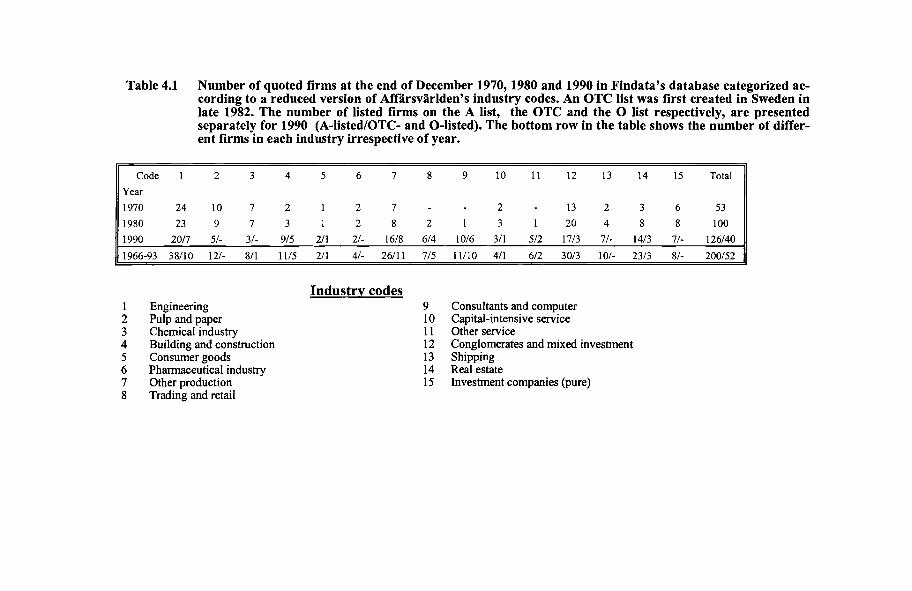
Table 4.1 Number of quoted firms at the end of December 1970, 1980 and 1990 in Findata's database categorized according to a reduced version of Afrarsvarlden's industry codes. An OTC list was first created in Sweden inlate 1982. The number of listed firms on the A list, the OTC and the 0 list respectively, are presentedseparately for 1990 (A-Iisted/OTC- and O-listed). The bottom row in the table shows the number of different firms in each industry irrespective of year.
Code 1 2 3 4 5 6 7 8 9 10 11 12 13 14 15 Total
Year
1970 24 10 7 2 1 2 7 - - 2 - 13 2 3 6 53
1980 23 9 7 3 1 2 8 2 1 3 1 20 4 8 8 100
1990 20/7 5/- 3/- 9/5 2/1 2/- 16/8 6/4 10/6 3/1 5/2 17/3 7/- 14/3 7/- 126/40
1966-93 38110 12/- 8/1 11/5 2/1 4/- 26/11 7/5 11/10 411 6/2 30/3 10/- 23/3 8/- 200/52
12345678
EngineeringPulp and paperChemical industryBuilding and constructionConsumer goodsPharmaceutical industryOther productionTrading and retail
Industry codes9 Consultants and computer10 Capital-intensive service11 Other service12 Conglomerates and mixed investment13 Shipping14 Real estate15 Investment companies (pure)

Accounting Information and Stock Prices
Appendix E contains a description of an additional procedure that was performed in order to check that the individual firm had not been incorrectlyclassified. This procedure led to the reclassification of a few firms that obviously had changed main business activity over the years, and it led to theintroduction of an additional industry category-building, construction andreal estate---containing the firms that could neither be classified as purebuilding and construction firms nor real estate firms.2
The final sample contains, in terms of finn-years, at least 75% of the total(1966 to 1993) population offirm-years.3 The absence ofbanks and the lossof nine trading and retail companies means a slight under-representation offirms with a particularly low expected accounting measurement bias (PMB).The limited number of observations in some industries, obviously, makesstatistical inferences related to that particular industry difficult. The industryclassifications, however, are mainly meant to guide the separation of firmsinto different sub-groups related to expected PMBs and expected validity ofhistorical ROE as a base for predictions. Also, the fact that the compositionof firm types included in the sample varies somewhat over the years will tosome extent make it difficult to produce unbiased comparisons of regressionresults for different time periods. This problem can probably be reduced,first of all, via the explicit inclusion of an estimated PMB in the regressionspecifications, but also via a careful choice of sub-sample compositions.
2
3
Appendix F summarizes the final number of firms in each industry at the end of December each year. The most important reason for the fewer observations, as comparedto the initial sample presented in table 4.1, can be traced to the calculation of data usingopening period capital. This means that the earliest observation for each firm is lost.It must be remembered that the largest loss of firms is related to the criterion requiring aminimum number of years on the stock exchange.
112

Sample Selection and Measurement of ...
4.2 The measurement of current ROE, the estimationof required return and the prediction of futureROE
In order to run empirical tests of the regression specifications proposed inthis study, a number of variables have to be specifically measured. Thissection will deal with three such issues, namely:
1. how to measure ROEj,t and shareholders' equityj,6
2. how to estimate Pj,6
3. how to estimate Et[ROEj,t+ 1].
4.2.1 Measurement of earnings, shareholders' equity and ROE
In this study, ROE for one period will be used as the base for the predictionof the level of ROE expected for the next period. The definition of ROEshould thus be chosen to ensure that it is a reasonable indication of thefinn's current ability to generate a profit. This naturally means that anearnings measure before e~traordinary items is preferred (assuming that thisis a transitory item).4 Given this study's focus on the firm's value and valuechange on the stock market, it is obvious that an earnings measure excludingminority interest is preferred. It is also clear that an earnings measure aftertax is desired, preferably with tax consequences arising from extraordinaryitems excluded. Two tax-related problenls arise: one relates to disclosurepractice, and the other to the treatment of the tax consequences associatedwith the changes in untaxed reserves (when openly disclosed). Appendix Gcontains a brief description of how Swedish practice concerning measurement of earnings and return on equity has changed over time.5 The development is illustrated separately in terms of recommendations, practice inannual reports, practice in the financial press, and empirical accounting research practice.
4
5
Given a longer term measurement perspective, it would be essential that all items wereaccounted for. This would lead to a preference for an earnings measure including extraordinary items. The change in book value of equity will, of course, be affected by allevents, even if they are classified as extraordinary.See also, Johansson (1984) for a discussion of the measurement of deferred taxes infinancial ratios.
113
5 Runsten

Accounting Information and Stock Prices
4.2.1.1 Chosen definition ofearnings
In line with both research practice (Bertmar and Molin, 1977 and Skogsvik,1988) and later recommendations by NBK (1983) and SFF (1985), earningsafter financial items (before extraordinary items), excluding minority shareof earnings, but including any earnings share of associated companies willbe used. Tax expenses will be calculated according to the comprehensive taxmethod with yearly estimates of the tax rate. Note that especially until thenlid 1970s, several firms did not openly disclose their annual and accumulated allocation to untaxed reserves. Tax consequences related to extraordinary items should ideally be controlled for. Given the typical lack of differentiated disclosure of this item and the lack of such disaggregation in Findata's database, an approximation is the best available alternative. The simplest approximation would be to multiply net extraordinary items by the taxrate and thus implicitly assume full taxation and full deductibility of all extraordinary items. However, given that the tax rate on many extraordinarygains has been relatively low and that several extraordinary costs have notbeen tax deductible, an approximation of this kind will overstate the taxconsequences related to extraordinary items. A simple (although not perfect)way to reduce the magnitude of this error is to use only half the tax rate onnet extraordinary items.
4.2.1.2 Chosen definition ofequity
The choice of opening period ex-dividend equity is consistent with thespecification of the valuation model being used in this study. Calculatingequity as disclosed shareholders' equity (excluding minority equity) plusuntaxed reserves minus a deferred tax liability (calculated at the estimatedyearly tax rate)6 is consistent with both the chosen earnings definition andwith the NBK and SFF recommendations.
6 Since it has been possible in Sweden, to defer tax. payment over substantial time periods, the use of the full tax rate will to some extent naturally overstate the deferred tax.liability (and thus understate the value of equity). This matter will be addressed laterwhen PMBs are to be calculated.
114

Sample Selection and Measurement of ...
4.2.1.3 Operationalization ofthe chosen definitions
The main definitions of earnings, equity and ROE can be summarized asfollows: 7
Earningst (~)
Earnings after fmancial itemst A
- (Allocation to untaxed reservest· 1:t )
- Taxes payablet A
+ (Extraordinary itemst· 1:t . 0.5)
- Minority share of earnings after tax
Disclosed shareholder's equityt-l
+ Taxed reservest_l A
+ Untaxed reservest_l (1 - 1:t )
- Proposed dividendt_l
X· tROE· t =_J_,_
J, Bj,t-l
To test whether the regression results are likely to be affected by the chosendefinition of ROE, the level and co-variability of three alternative specifications of ROE have been compared to the main specification for the entiresample of firms (the main ROE specification has been called ROEA). Tomeasure the effect of the rather arbitrarily chosen half tax rate on extraordinary items, an alternative ROE has been calculated assuming full taxation(ROEA). Furthem10re, given the wide-spread use of earnings and ROEcalculations according to the proxy-tax method (especially in the earlyperiods), such an ROE alternative has also been calculated (ROEB). Finally,an ROE specification after extraordinary items and comprehensive tax hasbeen calculated (ROEC). These alternative earnings measures can besummarized as follows:
7 Appendix H shows the principle layout of the income statement and balance sheet thatthese definitions are based on.
115

Accounting Information and Stock Prices
(X tA')Eamingst' Earnings? (xl)
Earnings after fmancial itemst "-
- (Allocation to untaxed reservest' Tt )
- Taxes payablet "-+ (Extraordinary itemst' Tt )
- Minority share of earnings after taxt
Earningsf (xF)Earnings after extraordinary itemst "
- (Allocation to untaxed reservest' Tt)
- Taxes payablet
- Minority share of earnings after taxt
Earnings after fmancial itemst · (1 - Tt )
- Minority share of earnings after taXt
The operationalization of these ROE definitions in terms of variables inFindata's database are presented, along with a discussion of some computing issues, in appendix I.
4.2.1.4 Measurement ofthe annual tax rate
Angelin and Jennergren (1994) provide a concise description of the development of the Swedish company tax rates:
"Until 1984, companies paid a municipal income tax finallyaveraging around 30% of taxable income. The previous year'smunicipal income tax was deductible from taxable income incomputing the state tax in the following year. The state tax was40% until 1983, 32% in 1984, and 52% between 1985 and 1988(the increase in 1985 was intended to compensate for theelimination of the municipal income tax at the end of theprevious year). Between 1989 and 1990, it was 40%. From 1991,it was 30%, as a result of the tax reform. Recently, it waschanged to 28% (from 1994). "
Angelin and Jennergren (1994, p. 8)
In line with common practice,8 the combined tax rate for the yearspreceding 1984 has been estimated as follows:
8 See e.g. Bertmar and Molin (1977).
116
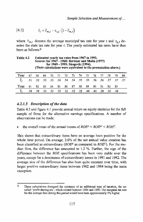
Sample Selection and Measurement of ...
[4:1]
where rm,t denotes the average municipal tax rate for year t and £s,t denotes the state tax rate for year t. The yearly estimated tax rates have thusbeen as follows: 9
Table 4.2 Estimated yearly tax rates from 1967 to 1993.Source: for 1967 - 1968: Bertmar and Molin (1977)
for 1969 - 1993: Skogsvik (1994).(Their calculations were equivalent to the presentation above.)
Year 67 68 69 70 71 72 73 74 75 76 77 78 79 80"'-
.51 .52 .52 .53 .54 .54 .54 .55 .55 .56 .56 .57 .57 .57£t
Year 81 82 83 84 85 86 87 88 89 90 91 92 93"'-
.58 .58 .58 .53 .52 .52 .52 .52 .40 .40 .30 .30 .30£t
4.2.1.5 Description ofthe dataTable 4.3 and figure 4.1 provide annual return on equity statistics for the fullsample of firms for the alternative earnings specifications. A number ofobservations can be made:
• the overall mean of the annual means ofROEA < ROEA' < ROEe.
This shows that extraordinary items have on average been positive for thewhole time period. On average, 2.6% of the net annual value creation hasbeen classified as extraordinary (ROEA as compared to ROEC). For the median firm, the difference has amounted to 1.2 %. Further, the sign of thedifference between the ROE specifications has been very stable over theyears, except for a dominance of extraordinary losses in 1991 and 1992. Theaverage size of the difference has also been quite constant over time, withlarger positive extraordinary items between 1982 and 1984 being the mainexception.
9 These calculations disregard the existence of an additional type of taxation, the socalled 'profit sharing tax', which existed between 1984 and 1990. The marginal tax ratefor the average firm during this period would have been approximately 5% higher.
117

Accounting Information and Stock Prices
• the overall mean of the annual means ofROEA > ROEB
The proxy tax ROE has, on average, been 1.8% lower than the ROE according to the comprehensive tax specification (ROEB as compared toROEA). This means that the calculated average comprehensive tax rate hasbeen lower than the marginal tax rate. This can consistently be observedduring the whole period, except again for the very poor years of 1991 and1992.
• the overall mean of annual std(ROEB)< std(ROEA)< std(ROEC).
Perhaps not surprisingly, return specification C that measures earnings including extraordinary items (ROEC) has been more variable than the returnspecifications measuring earnings before extraordinary items. The fact thatthe ROE specification measured after a proxy tax has been more stable(within each year except 1984) than the return specification that measuresearnings after comprehensive tax, can probably (essentially) be explained bythe differences in tax rate levels. Any extreme return level before tax issomewhat normalized by the higher proxy tax rate. The imperfect calculation of tax consequences on extraordinary items, according to the chosenspecification, can further result in a variation 'spill-over' effect on the ROEmeasure.
The only difference between ROEA and ROEA' concerns the tax calculationrelated to extraordil1ary items. This difference generates a 1.0% differencein the overall average ROE.
118

Sample Selection and Measurement of ...
Table 4.3 The annual median, mean and standard deviation of fourdifferent specifications of ROE for a sample of 252 listed Swedishfirms from 1967 to 1993. The number of firms each year isspecified in the last column. For details regarding the ROE definitions, see Section 4.2.1.4.
ROEA ROEA' ROEB ROECYear Mrlim Mean Std MOOial Mean Std Mrlim Mean Std MOOin Mean Std n1967 6.7 6.6 6.0 7.0 7.2 5.4 4.7 5.5 5.2 7.5 8.3 5.1 391968 8.8 9.5 7.4 8.9 10.4 7.5 6.6 7.3 6.3 10.7 12.1 10.4 391969 9.4 10.8 8.0 10.2 11.9 8.5 7.5 8.8 7.3 11.2 13.8 11.4 421970 9.0 8.9 5.6 9.1 9.4 5.4 7.5 7.8 4.7 9.5 10.4 6.3 431971 9.0 8.7 5.8 9.1 9.2 5.6 6.2 6.4 4.7 9.6 10.2 6.2 701972 9.3 9.9 7.7 10.0 10.7 8.2 6.8 7.1 5.8 10.8 12.1 10.3 721973 14.4 14.2 8.9 15.1 15.3 8.8 10.9 11.3 6.6 15.7 17.2 10.7 761974 17.5 17.9 12.2 17.8 19.2 11.8 13.5 15.7 10.7 18.4 21.3 13.3 791975 12.0 11.1 11.1 12.5 12.7 11.1 9.3 9.0 9.2 13.5 15.1 12.5 771976 10.5 10.1 13.7 11.4 10.9 13.8 7.5 7.2 9.3 11.6 12.2 14.8 831977 7.3 4.5 15.2 7.7 5.1 15.0 5.0 3.4 10.0 7.8 6.2 15.3 861978 8.1 4.7 16.9 8.4 5.0 17.6 4.6 3.4 11.2 8.8 5.4 20.0 881979 11.2 10.5 12.2 11.8 11.8 12.7 8.0 8.4 8.9 12.2 13.6 18.7 891980 11.3 11.3 14.1 11.6 12.7 11.2 9.2 9.1 10.0 12.4 14.8 11.1 911981 11.9 12.0 12.8 12.9 13.6 12.5 7.7 8.5 9.4 14.2 15.9 13.7 921982 11.3 11.9 18.5 11.9 14.4 22.3 7.8 8.7 12.3 13.1 18.0 30.7 951983 13.9 13.5 17.2 14.8 17.8 19.3 10.9 11.4 13.2 16.4 23.9 26.4 961984 16.9 18.0 22.4 18.1 19.9 22.2 13.4 16.1 23.6 19.6 23.2 25.2 1521985 13.5 14.7 11.7 14.4 15.9 12.2 12.2 12.9 10.7 15.6 18.0 16.0 1611986 14.5 15.8 23.2 15.0 16.9 22.9 12.6 14.3 21.6 16.6 19.0 23.8 1641987 15.2 15.0 12.3 16.2 16.0 13.3 12.8 12.8 10.5 15.9 17.9 19.9 1691988 17.2 18.9 29.2 18.0 20.0 28.1 13.7 15.4 18.9 19.0 22.1 28.3 1681989 17.3 18.8 18.5 17.7 20.0 19.8 15.3 16.7 15.6 19.6 23.4 26.8 1661990 11.8 11.3 18.4 12.5 11.4 19.0 10.6 10.7 14.0 12.9 11.8 23.6 1521991 3.5 2.7 16.1 3.6 2.1 17.2 4.1 3.5 13.9 3.4 -0.5 27.9 1311992 1.2 -4.5 23.6 1.0 -5.0 24.3 1.7 -2.5 18.8 0.2 -7.3 30.8 1201993 8.4 7.3 24.5 8.4 7.4 24.5 6.1 6.1 20.1 8.5 7.4 26.8 108Mean 11.2 10.9 14.6 11.7 11.9 14.8 8.8 9.1 11.6 12.4 13.5 18.0 102
119

Accounting Information and Stock Prices
Average ROE with different earnings specifications
25% -r-"----------------------...../'-\
20% -I-------~------____i'--~t___----L--4_----I
15% +--------#---I-~~---___=_"--_#_~~--""oo~<----_=:H_----1
5% +--------------L.J~~----------........t_--JI
0% -I--------------------__~~~
-5% +- ~--1
-10% +--+----1--+----+---+--+-..--+--+--+---+--+--I--+--+--+--+--+--+---+--+--+--I--+----+---+----467 68 69 70 71 72 73 74 75 76 77 78 79 80 81 82 83 84 85 86 87 88 89 90 91 92 93
1--ROE(A) ••••••ROE(B) - - - ROE(C) I
Figure 4.1 A graphical illustration of the annual mean ROE for the sample of252 listed Swedish firms from 1967 to 1993 given three differentearnings specifications.
The choice of ROE specification can naturally be expected to affect the sizeof a in the regression specifications to some extent. If the magnitude of theslope-coefficients in the regression models is likely to be affected by thechoice of the ROE specification, can better be analyzed by studying the covariability of the different ROE specifications. Do all ROE specificationstell the san1e story? In table 4.4, the correlation between ROEA and the threealternative specifications is presented for each year.
120

Sample Selection and Measurement of ...
Table 4.4 Pairwise annual correlation between the main ROE specificationand three alternative specifications.
Annual correlation coefficientsYear ( A A') (ROE!,1;ROE~t ) (ROEft;ROEJ,I ) nROEj,t;ROEj,t
1967 0.98 0.94 0.78 391968 0.92 0.89 0.57 391969 0.94 0.92 0.70 421970 0.96 0.92 0.72 431971 0.96 0.86 0.74 701972 0.95 0.88 0.75 721973 0.94 0.89 0.68 761974 0.96 0.91 0.73 791975 0.97 0.91 0.82 771976 0.99 0.94 0.92 831977 0.99 0.95 0.95 861978 0.98 0.95 0.88 881979 0.86 0.93 0.48 891980 0.94 0.92 0.46 911981 0.96 0.83 0.78 921982 0.94 0.85 0.80 951983 0.92 0.88 0.70 961984 0.97 0.96 0.79 1521985 0.95 0.89 0.71 1611986 0.99 0.93 0.90 1641987 0.90 0.86 0.57 1691988 0.99 0.95 0.89 1681989 0.98 0.96 0.83 1661990 0.99 0.96 0.84 1521991 0.98 0.95 0.72 1311992 0.99 0.97 0.87 1201993 1.00 0.98 0.91 108Mean 0.96 0.92 0.76 102
The correlation between ROEA and ROEA' is on average very close to 1.00(0.96), indicating that the choice between these two specifications might beof little importance for the magnitude and significance of the estimatedslope-coefficients in the regression models. ROEB also tells a very similarstory, with an average correlation of 0.92. Naturally, the ROE specificationincluding extraordinary items 'tells a son1ewhat different story'-nevertheless, the average correlation is 0.76 for the whole time period.
121

Accounting Information and Stock Prices
4.2.2 Required rate of return or the cost of equity capitalEt[ROEj,t+l] is a key explanatory variable in this study. The estimated costof equity capital is used to calculate the sign and size of abnormal performance. The standard procedure in financial market research has been to estimate the market's required rate ofretum as a function of a risk-free interestrate plus a risk premium. Relying on the capital asset pricing model(CAPM), COIT'.J11on research practice has been to use a finn-specific risk parameter such as beta. Unfortunately, estimated historical betas have provedto be empirically ratl1er weak as tl1e explanatory variable for equity return. 10
Different portfolio approaches and estimation refinements have been proposed to mitigate the estimation problems. ll The literature suggests a number of alternative routes for measuring risk. These include betas estimatedutilizing accounting data,12 several multi-dimensional risk modelsemanating from the arbitrage theory of asset prices (APT, Ross 1976),13 andindustry-factor betas.14
It is beyond the scope of this study to evaluate the 'best' risk differentiationmethodology. The common approach that uses a finn- and time-specificestimate of beta based on historic market movements will thus be used asthe main alternative. Findata's 48 month market beta will be used.l5 Someof the initial tests, will also be performed assuming no firm-specific riskdifferentiation at all (i.e. beta = 1 for all firms), in order to gain someindication of the consequences of this choice.
The main cost of equity capital specification can thus be described as follows:
[4:2]
10
1112
131415
See e.g. the following studies: Reinganum (1981), Lakonishok and Shapiro (1986) andFama and French (1992).See e.g. Blume (1970) and Fama and MacBeth (1973).See e.g. Beaver, Kettler and Scholes (1970) and Rosenberg and Guy (1976a and1976b).See e.g. Chen, Roll and Ross (1986) and Roll (1988).See e.g. Kale, Hakansson and Platt (1992).Monthly firm return is compared to changes in "Affarsvarldens generalindex" (AGI).This is a value weighted index based on all firms listed on the Stockholm Stock Exchange.
122

Sample Selection and Measurement of ...
where
P" = The estimated cost of equity capital for firm} at the end ofperiod t.j,t
fit The risk-free interest rate at time t.
rp = The estimated risk premium.
P" = Findata's 48 month market beta for firm)· at the end ofperiod t.j,t
The estimation of the risk-free interest rate and the level of the general riskpremium is the topic of the following paragraphs.
In figure 4.2, the Swedish long-term risk-free rate of interest has been plotted over time. The Swedish money market was heavily regulated until theearly 1980s.16 Treasury notes were not introduced until 1982. In the fall of1983, the National Bank of Sweden abolished some of the placement restrictions on Swedish banks. A year later, restrictions on insurance companieswere also eased. Until then, the second-hand market for long-term government bonds was almost nonexistent. Thus the rates that were published before 1983 in the National Bank's Statistical Yearbook are to some extenthypothetical rather than based on actual trade. Furthermore, the availableterm structure of the bonds has changed over time; in some years orlly oneof the 5, 10 or 15-year bonds has existed. The annual changes of theSwedish Consun1er Price Index have also been plotted in figure 4.2. As canbe seen from the figure, there seems to have been a fairly consistent positivemargin of about 3-5% between the actual rate of inflation and the interestrate after 1982. The pattern is less clear for the years leading up to 1982;there are several years of zero margins and even negative margins. Whatwas the investor's true risk-free alternative? When performing a study of theSwedish n1arket in the 1960s and 1970s, it is not obvious which risk-freeinterest rate one should use. However, in this study published long-termgovernment bond rates will henceforth be used.
16 See Kvist, Nyberg and Wissen (1985) for a more complete discussion of the development of the Swedish money market.
123
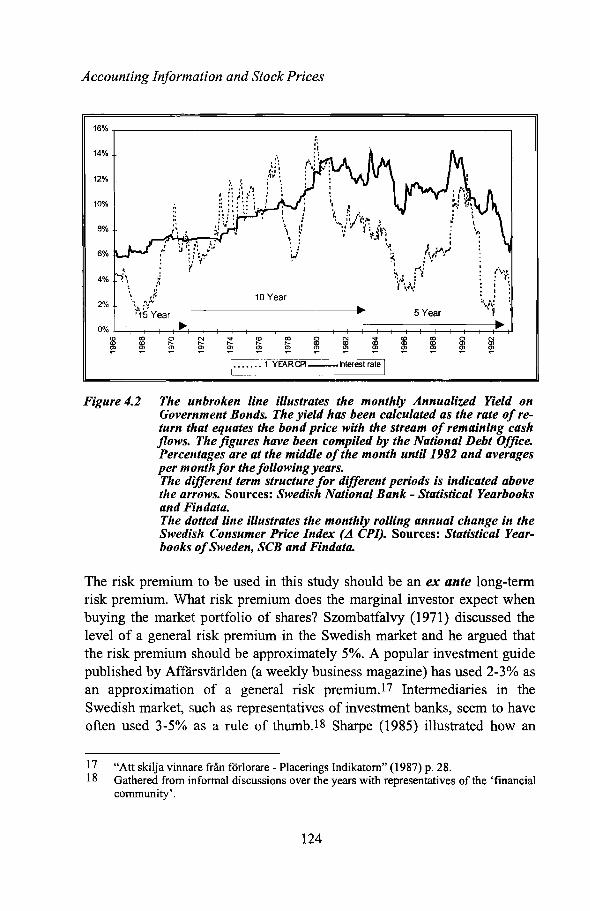
Accounting Information and Stock Prices
16% -r------------------------------.
oex>0)
.~~~~ ~ ~·lv.: It. \..
to......0>
10 Year
-----------~~ 5 Year
o N...... ......0) 0)
ex>to0)
0% +-+-t--+--t--=~__t___!__+__+__t__+__+__+___+__+_+_+__+__+__+__~f____if____i____+____+--+__+'toto0)
8%
6%
10%
12%
14%
1....... 1 YEARCA--nterestrate I
Figure 4.2 The unbroken line illustrates the monthly Annualized Yield onGovernment Bonds. The yield has been calculated as the rate of return that equates the bond price with the stream of remaining cashflows. The figures have been compiled by the National Debt Office.Percentages are at the middle ofthe month until 1982 and averagesper month for the following years.The different term structure for different periods is indicated abovethe arrows. Sources: Swedish National Bank - Statistical Yearbooksand Findata.The dotted line illustrates the monthly rolling annual change in theSwedish Consumer Price Index (A CPI). Sources: Statistical Yearbooks ofSweden, SCB and Findata.
The risk premium to be used in this study should be an ex ante long-termrisk premium. What risk premium does the marginal investor expect whenbuying the market portfolio of shares? Szombatfalvy (1971) discussed thelevel of a general risk premium in the Swedish market and he argued thatthe risk premium should be approximately 5%. A popular investment guidepublished by Affarsvarlden (a weekly business magazine) has used 2-3% asan approximation of a general risk premium.17 Intermediaries in theSwedish market, such as representatives of investment banks, seem to haveoften used 3-5% as a rule of thurrlb.l 8 Sharpe (1985) illustrated how an
17 "Att skilja vinnare fran f6rlorare - Placerings Indikatom" (1987) p. 28.18 Gathered from informal discussions over the years with representatives of the 'financial
con1ffiunity' .
124

Sample Selection and Measurement of ...
American brokerage firm made projections of the risk premium. Theestimates he provided indicate an expected risk premium for stocks for theperiod 1967-1984 of2-7%.19
Studies of ex post risk premiums have generally used the annual change in amarket index and added dividends (assumed to be reinvested), and then deducted an approximation of the risk-free interest rate. Unfortunately, depending on the period being studied, these ex post averages tend to fluctuateimmensely. The results of some empirical studies performed on US andSwedish data are summarized in the tables below.
Table 4.5 Ex post risk premium for different periods in Sweden and the US.Long- and short-term refers to the term structure of the risk-freealternative.
Period! type/ country Geometric Arithmetic Sourcemean mean
1926-87/ long-term! US 4.7% 6.8% Ibbotson & Sinquefield (89)1926-87/ short-term! US 6.2% 8.3% Ibbotson & Sinquefield (89)1926-87/ short-term! SW 5.6% 7.2% Frennberg & Hansson (91a)1919-89/ short-term! SW 4.4% 6.1 % Frennberg & Hansson (91a)1938-87/ short-term! SW 8.9% de Ridder (89)
Table 4.6 Ex post risk premium in Sweden first for separate decades, thenfor successively longer periods starting in 1919 using data pub-lished in Frennberg and Hansson (1991a).
Period Geometric Arithmetic Period Geometric Arithmetic Yearsmean mean mean mean
1919-29 -3.7% -2.3% 1919-29 -3.7% -2.3% 111930-39 -3.3% -0.7% 1919-39 -3.5% -1.5% 211940-49 7.4% 7.7% 1919-49 -0.1% 1.4% 311950-59 12.3% 13.6% 1919-59 2.8% 4.4% 411960-69 2.8% 3.9% 1919-69 2.8% 4.3% 511970-79 0.1% 1.3% 1919-79 2.3% 3.8% 611980-89 17.6% 19.9% 1919-89 4.4% 6.1% 71
The ex post calculated risk premium is apparently very sensitive to whichperiod is chosel1 for study (and how it is calculated). That is, of course, the
19 See figure 20-16 in Sharpe (1985).
125

Accounting Information and Stock Prices
very essence of risk. It is not known in advance what the return will eventually be. Apparently, even for a two-decade period, a portfolio of stocks mayperform worse than the same period's risk-free alternative. Ibbotson andSinquefield (1989) argued that the risk premium follows a random walkimplying that the longest possible historic average is expected to be the bestestimate. Using a probabilistic view ibid. (p. 125) further argued that anarithmetic mean should be used in future-oriented estimations of the cost ofcapital. Scott (1992 and 1993), however, agreed with neither Ibbotson andSinquefield's calculations nor their conclusions:
HIn conclusion, 8 per cent per annum is far too big an estimateofthe risk premium on equities, both because it relies on too bigan estimate ofthe expected mean return on equities, and becauseit relies on too small an estimate ofthe 'riskless' rate ofreturn. "
Scott (1993, p. 64)
Scott (1992) pointed at two crucial assumptions that must be satisfied forthe arithmetic mean to be the relevant base for a risk premium estimate.
HThe crucial assumptions are:1. That past annual returns are a random sample of returns
which are to be expected in the future;2. That each annual return is drawn independently from the
population ofpossible returns. "Scott (1992, p. 23)
Scott (1993) later concluded:
HThe arithmetic mean would, nevertheless, be a better estimateof the future mean expected return if annual return could be regarded as independent drawings from a population. However, Iargue that investors are more likely to form their expectations onthe basis ofcurrent dividend yields and expected growth rates ofdividends, and these do not behave in a random manner, and doconform to the geometric mean. "
Scott (1993, p. 64)
Ibbotson and Sinquefield (1989) pointed out that the serial correlation between successive annual returns on equity had been approximately zero.Poterba and Summers (1988), however, identified a long-term mean reversion tendency in the development of US stock market prices. Frennberg and
126

Sample Selection and Measurement of ...
Hansson (1991b), studying Swedish stock market prices over the period1919 to 1990, also found a long-term mean reversion tendency in pricedevelopment. Clinebell, Kahl and Stevens (1994) studying US data found anauto-regressive risk premium for 1926-58, but a random variation around amuch lower mean risk premium for 1959-1990. In line with Scott'sargumentation, and stating that: "historical observations are notindependent draws from a stationary distribution", Copeland, Koller andMurrin (1991, p. 193) recommend the use of the geometric mean as the bestestimate of an equity risk premium.
The valuation model presented in this study relies on the discounted valueof a long lasting stream of future dividends. For a long-term estimate of thecost of equity capital, tl1e chance that the arithmetic mean calculated riskpremium overstates the expected cost of capital seems to be rather high.Further, the level of the long-term geometric mean is more consistent withaculal observations, admittedly anecdotal, of ex ante risk premiums. For thelongest periods studied, the geometric mean varies between 4 and 6 percent.A risk premium of 5 percent will henceforth be used as the estimate of themarket general risk premium in this study.
127

Accounting Information and Stock Prices
4.2.3 Prediction ofROE for the next period-conceptuallyA robust yet simple method to predict the next period's ROE, or ROE - p, isneeded for this study. The prediction procedure will be used for differentfirms over the whole 27-year period being studied, and while it needs to beas simple as possible, a number of criteria need to be fulfilled. The procedure needs to:1. be consistent with the specification of the valuation model,2. be consistent with empirical observations,3. generate predictions that are reasonable approximations of investor's
expectations, and4. make adequate use of historical observations without preventing the
study of early time periods and firms with a limited history.
In the valuation model in Chapter 2, it was explicitly assumed that a firm'sreturn on equity could deviate from the market's expected return only for alimited period of time (in the absence of a persistent accounting measurement bias). ROE is, in other words, expected to move towards the marketcost of equity capital (P). The underlying forces were assumed to be competition and a struggle to survive. Monopoly or monopoly-like situations, dueto, for example, patents or high barriers to entry, could be one explanationfor persistent or slowly diminishing abnormal return. Given competition anda constant cost of equity capital, one would thus expect an ideally measuredROE to move towards the cost of capital. A process where ROE graduallymoves towards p over time was expressed in a previous section as follows:
where 0 ~ A< 1
Lambda is a 'fading' factor, deciding the speed of the reversion process.
A vast number of studies have been carried out to test the predictive abilityof different forecasting approaches for accounting earnings. Formal studiesof the time series behavior, and the ability to forecast profitability ratios(e.g. ROE) are, on the other hand, relatively scarce. Below follows a briefreview of the results.
128

Sample Selection and Measurement of ...
4.2.3.1 Earnings forecasts
Foster (1986) discussed alternative forecasting approaches and classifiedthem in two times two dimensions: mechanical versus non-mechanical approaches, and univariate versus multivariate approaches.
Table 4.7 Classification of forecasting approaches, from Foster, 1986, Table8.1.
Univariate Multivariate
Mechanical Moving average models Regression modelsBox-Jenkins models Box-Jenkins models
Econometric models
Non-mechanical Visual curve extrapolation Security analyst approach
4.2.3.1.1 Univariate mechanical approaches
Authors of several studies have tried to identify the statistical process thatbest captures the earnings generation process. A univariate approach usesonly the historical development of the variable being studied. The submartingale process has been found to most successfully capture the statisticalproperties of the earnings generation process for a randomly selected sampleof companies.20 A time series that follows a submartingale process canmathematically be expressed as follows: 21
where t/J = 1 and t5 ~ O. In a pure martingale process t/J = 1 and t5 = o. Translated to an earnings measure, the best guess of next period's earningsequals, according to the pure process, the earnings most recentlydisclosed.22 The t5 parameter captures an expected growth in the variable
20
2122
Ball and Watts (1972) is an example of an early study of the earnings generation process. Watts and Zimmerman (1986) provide a good review of the field.The notation in this section follows Foster (1986) p. 232.In the accounting literature, the martingale process is often also referred to, even thoughit is really more restrictive, as the random-walk. If the error terms (St,Et+l, .... Et+n) ofa
129

Accounting Information and Stock Prices
over time, and St is a random variable with an expected zero mean. Whenan absolute nominal earnings measure is used, 0 is expected to be largerthan zero, due to, for example, inflation, reinvestment of earnings andacquisitions. Several studies, including Watts and Zimmerman (1986), haveshown that this is the most successful univariate process in describingearnings changes for a 'normal' sample. Brooks and Buckmaster (1976,1980) have, on the other hand, illustrated that if a sample of extreme firms ischosen (i.e. firms with extreme values of earnings in the last period), aprediction model that assumes that the level of earnings returns to the preextreme level is more successful than the submartingale model.
The focus in the US has often been on quarterly earnings. It is natural thatdifferent methods for seasonal adjustments have been used under such circumstances. The Box-Jenkins methodology has successfully been used tofirst identify a seasonal pattern and thereafter to estimate a function thatexploits all the information in the time series. Firm specific models are estimated and parameters for auto-regression and/or moving averages are generated. This approach has generated better predictions in tests (smaller prediction errors) than the submartingale method.23 However, the estimatedparameters often lack any economical interpretation, and also tend to beunstable both over time and between different samples of firms.
4.2.3.1.2 Multivariate mechanical approaches
Using a multivariate forecasting approach, the dependent variable is thoughtto be a function of several explanatory variables. This approach has beencommon in, for exan1ple, the construction of econometric models forecasting the development of the whole economy or an industry, and for bankruptcy prediction. However, it has been less commonly used for predictingfuture company earnings, Ou (1986) being an exception. Ou constructed alogit-model for the prediction of next year's earnings change. From a list ofmore than sixty accounting numbers and ratios, eight ratios were selected.The predictive performance of the logit-model was subsequently compared
23
series are independent and identically distributed, the series is said to follow a stochastic process called the random-walk. This process is often used to describe the behaviorof changes in stock market prices. See e.g. Copeland and Weston (1988).See e.g. Foster (1986).
130

Sample Selection and Measurement of ...
to four earnings-based models.24 Especially when there were large earningschanges, Ou's prediction model was found to make more accurate predictions than the other four models.
4.2.3.1.3 Non-mechanical approaches
The earnings predictions that security analysts provide are typical of thenon-mechanical forecasting approach. Many factors, such as expectationswith regard to the business climate, the development of interest rates, quotations by managements, and disclosed accounting infornlation are presumably combined into a firm-specific forecast in an approach of this kind.Sometimes expectations are formed for a specific parameter, such as nextyear's earnings, and made public in business magazines. In Sweden, earnings per share predictions (for the next accounting year) have been published in Affarsvarlden (since 1973) and in Veckans Affarer (since 1974).Other actors, such as financial research departments of investment banksand brokerage firms, also produce firm-specific forecasts. Whether theseforecasts are better than the mechanical forecasts is an empirical question,but since they are costly to produce and very much in demand, it appearsthat they might be considered superior.
Brown and Rozeff (1978) have nlade formal evaluations of the predictionperformance of analysts. With a random sample of 50 firms, the predictionperformance of three time series models25 was compared to forecasts published by Value Line.26 They concluded that the security analyst approachwas superior to all the tested time series models. Brown, Griffin, Hagermanand Zmijewski (1984) drew equivalent conclusions. They studied 233 firmsover the period 1975-80, using three different univariate Box-Jenkins models. Again, Value Line was used as a proxy for security analyst's forecasts.Liljeblom (1989) studied 89 stocks listed on the Stockholm Stock Exchangeduring the period 1977-1984. Studying EPS, Liljeblom compared the forecasting performance of a random-walk model against published forecasts in
24
25
26
A random guess prediction, a trend model, a reversal model and a model based onBrooks and Buckmaster.The time series models that were used were a seasonal adjusted martingale, a seasonaladjusted submartingale and a Box-Jenkins model.Value Line Investment Survey published earnings forecasts for 1,600 American firms.A forecast for the next five quarters was published weekly.
131

Accounting Information and Stock Prices
the business weekly Veckans Affarer. She concluded that the forecasts provided by the business magazine significantly outperformed the naive forecasts given by the random-walk model.
Foster (1986) concluded that an important reason for the forecasting superiority of the security analysts is probably their use of a broad infornlation set.
A more formal evaluation of the multivariate mechanical approach versusthe security-analyst approach has not been found in the literature.
4.2.3.1.4 Conclusions regarding the earnings process
• Earnings changes cannot generally be predicted by current and pastearnings. (Ball and Watts [1972])
• Extreme levels of earnings tend to be followed by more normal earnings.(Brooks and Buckmaster [1976, 1980])
• In comparison with the sub-martingale prediction approach, the BoxJenkins methodology has shown a better ability to identify additionalpredictive power for a firm-specific time series.
• Security analysts seem to generate more accurate forecasts than the univariate time series approaches. (Brown and Rozeff [1978], Brown,Griffin, Hagerman and Znlijewski [1984] and Liljeblom [1989]).
• More accurate predictions can be expected to be generated by adding abroader set of accounting variables to the mechanical approach. (Ou[1986])
4.2.3.2 Return on equity forecasts
Foster (1986) noted that little evidence has been published on the time seriesbehavior of financial ratios. Freeman, Ohlson and Penman (1982) rejectedthe hypothesis that ROE follows a random walk. They evaluated the correlation between (ROEt+1 - ROEt) and ROE!, and interpreted the negativecorrelation they found as an indication of a nlean-reversion process, that is,extreme ratios tend to be followed by normal ones. Freeman, Ohlson andPenman (1982) noted that the results in Beaver (1970) and in Lookabill(1976) also support the hypothesis of a mean-reversion process. However,they did not discuss to what mean ROE can be expected to move. The idea
132

Sample Selection and Measurement of ...
of a nlean reversion process is obviously also consistent with the behaviorof extreme earnings documented in Brooks and Buckmaster (1976,80). In asample ofDS firms, Ou and Penman (1994) observed that the ROE ratio hasbeen positively serially correlated and mean reverting; further the reversionprocess has been slow (lasting over many years), and the ROE ratio of different portfolios of firms had apparently not converged to the same mean.The latter is, for example, consistent with the presence of a persistent accounting measurement bias that affects different types of firms differently.Ou and Penman (1994) further noted that the tendency of mean reversionhas been nluch stronger for relatively low and high levels ofROE.
Statistical conclusions regarding the ROE process• Rather strong positive one period auto-correlation.• Slow mean reversion tendency.• All firms' ROE do not seem to converge towards the same mean.• The reversion fronl extreme levels seenlS to be stronger.
133

Accounting Information and Stock Prices
4.2.3.3 Choice offorecasting approachAlternative prediction models that can be used in this study:
PI Et[ROEt+1] = ROEt
P2 Et[ROEt+1] = Pt + A[ROEt - Pt]
P3 Et[RDEt+l ] = Pt +a l .arctan[(ROEt - p}a2 ]
1 n
P4 Et[RDEt+l ] = - LROEt+I_in i=1
n
P5 Et[ROEt+1 ] = L{i)t+l-i . ROEt+1_i;=1
nwhere LaJt+l-i = 1
i=l
P6 Et[ROEt+1] =f{ROEt-n ~ ROEt}
P7 Et[ROEt +1] =f{Accounting line items}
P8 [ ] _ E/V[ROEt+l]+E;A[ROEt+t}Et R(JEt+1 - 2
1 n .
P9 Et[RDEt+1] = - LE:[ROEt+l ]n ;=1
Martingale
Mean reversion (MRP)
S-shaped MRP
Historical mean over nyears
Weighted historicalmean over n years
Estimated ARIMAmodel
Broad information set
Forecasts in businessmagazines27
Analysts' consensus;mean over n analysts
The first three models only exploit information in the most recent performance measure, whereas the next three use information from a number of historic periods. The last three models exploit a wider set of information, eitherin a mechanic prediction model or as manifested in expectations publishedin the financial press or provided by financial analysts. It is beyond thescope of this study to formally test the prediction performance of each ofthese models--one must, however, be chosen.
The first model (a martingale in ROE) is the simplest. Its major disadvantage is that it ignores the observed mean reversion tendency. However,looking just one period ahead, this might not be a severe problem if extreme
27 AV = Affarsvarlden and VA = Veckans Affarer.
134

Sample Selection and Measurement of ...
levels of ROE are controlled for. The MRP model does, on the other hand,specifically exploit the mean reversion tendency. It does not, however, takeinto account the observation that the mean reversion is stronger for the moreextreme levels of ROE. The S-shaped model (P3) is especially designed todeal with this problem.28 The use of several years of reported ROE in a prediction model can be expected to generate more stable predictions, but notnecessarily predictions with smaller prediction errors in a one-period-aheadcontext. The unweighted historic mean is often criticized for putting toolittle weight on the n10st recent observation. That problem is mitigated inthe weighted historic mean prediction model. A drawback inherent in bothof these methods is the need for access to data for many historic years.
The advantages of an ARIMA model are particularly obvious if a seasonalpattern is expected in the data. Such patterns can be expected to be ratherstrong in quarterly data, but as this study is based on annual data, the advantages of such a model specification seem limited.29
The scope of this study further rules out the estimation of a broad information based prediction model (P7). The lack of published forecasts in thebusiness press for the whole period being studied, eliminates the businesspress alternative (P8). The analysts' consensus database compiled byIIB/E/S unfortunately only includes Swedish firms from 1987 and onwards.
PI, P2 and P3 seem to best satisfy the simplicity and the 'low informationconsumption' criteria.
The specification of the S-shaped model needs further description. Theproperties of the trigonometric function arctan (the inverse tangent), is usedin P3 as a transformation function. Arctan has the properties of a first derivative that is positive for all values, a positive second derivative for negative values and a negative second derivative for positive values. These arethe properties of a positively sloping S-function.
28
29
Freeman and Tse (1992) successfully used a similar nonlinear model when they studiedsecurity price responses to unexpected earnings.Furthermore, the need for data for many historic years is a major drawback given thisstudy's purposes.
135

Accounting Information and Stock Prices
[4:4] y=arctan(x)
The slope of [4:4] is equal to one when x is close to zero. The followingboundary characteristics hold for the arctan function (see illustration infigure 4.3):
[4:5]
[4:6]
[4:7]
y = 0 when x = 0
1CY ~ - when x ~ 00
21C
y~-- when x~-oo2
y
+1t/2
---------#-------- X
-1t /2 . ..
Figure 4.3 Graphical illustration ofthe properties ofthe arctan function.
Incorporating parameters al and a2' yields the following function.
[4:8] y = al . arctan(x. a2)
The shape of the function can be altered by using different levels of the parameters (al and a2). The following characteristics hold for the transformedfunction:
i) the value of al· a2 is equal to the slope of the line close to the origin,
136

Sample Selection and Measurement of ...
ii) when al decreases the S-shape is more pronJunced,30iii) when a2 is close to zero, [4:8] is approximately linear.
Exchanging x for (ROE-p) generates the prediction model P3, which givencertain combinations of the parameters al and a2 may be equal to PI, P2 orsimply be consistent with accelerating mean reversion for extreme ROElevels.
• P3 is approximately identical to PI when ale a2 = I and a2 is very low(close to zero).
• P3 is approximately identical to P2 when ale a2 = Aand a2 is very low(close to zero).
• P3 is S-shaped when a2 is not close to zero, the maximum level of expected residual return is decided, regardless of the current level of ROE,by the level of ale (If, for example, aI=O.25 then maximum and
minimum EI[ROEI+1 ] =Pt ±0.25· ; ~ PI ±0.39 ).
al and a2 can thus, for example, be chosen to force the model to generateROE predictions that are equal to the martingale model (or the MRP model)when current ROE is close to p, and predictions with an increasing meanreversion tendency the further current ROE is from p. Concrete illustrationsof these properties follow below. Figure 4.4 illustrates current and predictedROE graphically given prediction models PI, P2 and P3 (with specific parameters).
30 The following boundary conditions hold for the transformed function:
y~al·!!... when x~CX) and y~-al·!!... when X~-OO2 2
137

Accounting Information and Stock Prices
30%
10%
-50% -40%> -300/0 -200/0 -1
-20%
-30%
-40%
-50%
30% 400k 500/0
ROEt - p
Figure 4.4 The relationship between current ROE-p and expected next periodROE-p for the Martingale model (PI), the Mean Reversion model(P2) with A. = 0.7, and the S-shaped model (P3) with aJ = 0.25 anda2 =4 (aJ . a2 =1.0) when p= 15%.
Table 4.8 illustrates the increasing and differing mean reversion speed fordifferent combinations of al and a2 and two examples of current ROE. Notethat when a2 is close to zero, the mean reversion tendency is constant for alllevels of ROE (a linear relationship). The reversion tendency is equal to0.90 (al· a2 = 'A). At the other extreme, when al is close to zero, the meanreversion tendency is complete; Et[ROEt+1] = Pt for all levels of currentROE (A. = 0.00). For all other parameter combinations, the mean reversiontendency increases the further ROE is from the expected norm (P). Forexample, given a combination of at = 0.3 and a2 = 3, the A.-equivalentequals 0.87 and 0.69 respectively, when current ROE equals 25% and 50%respectively.
138

Table 4.8
Sample Selection and Measurement of ...
A numerical illustration of the different degrees of mean reversionfor the S-shaped prediction model, given different combinations ofa1 and a2 and two examples of current ROE. Pt and at · a~ arefixed at 15% and 0.90 respectively. As the multiple (at· a2) In allcases is assumed to be a positive constant (0.90), at and a2 are assumed to only approach zero and infinity respectively, at each extreme of the table.
Et[ROEt+,]=pt +at·arctan[(ROEt -pt)·az]
Pt= 15 % & al·a2 = 0.90 ROEt = 25 % ROEt = 50 %
al a? E[ROEt+l] A-equivalent E[ROEt+l] A-equivalent~ co ~O 24.0% 0.90 46.5% 0.90
1.00 0.90 24.0% 0.90 45.5% 0.870.90 1.00 24.0% 0.90 45.3% 0.870.80 1.13 24.0% 0.90 45.0% 0.860.70 1.29 24.0% 0.90 44.6% 0.850.60 1.50 23.9% 0.89 44.0% 0.830.50 1.80 23.9% 0.89 43.1% 0.800.40 2.25 23.9% 0.89 41.7% 0.760.30 3.00 23.7% 0.87 39.3% 0.690.20 4.50 23.5% 0.85 35.1% 0.570.10 9.00 22.3% 0.73 27.6% 0.360.05 18.00 20.3% 0.53 22.1% 0.20
: :
~O ~ co 15.0% 0.00 15.0% 0.00
Estimating the parameters of the S-shaped model, using empirical data canbe viewed as a test of the relative statistical fit of PI, P2 and P3. Such anestimation can thus be used as a guide towards choosing the mostreasonable prediction procedure.31 However, before such estimations areperformed, the firm-specific PMBs must be estimated.
31 The estin1ation of the parameters for the S-shaped model is done in two steps. Searchthe value of a2 that maximizes the explanatory power of the following linear function:
• (ROEj,t-pj,r)=ao+at·Xj,t+~j,twhere
Xj,t == arctan[(ROEj,t - Pj,t)' a2]
If a permanent firm-specific return on equity measurement bias (Yj,t) is expected, an estimate of the bias is included in the estimation model:
• (ROEj,t - Pj,t - rj,t) =ao + at . Xj,t + ~j,twhere
Xj,t ==arctan[(ROEj,t -Pj,t -rj,t)·a2]
139

5 QPERATIONALIZATIONS
In the first section of this chapter a classification and quantification of thefirm characteristics discussed in Chapter 3 will be performed. Section 5.2presents an operationalization of the selected descriptors of change in theeconomic climate (related to the inflation rate and business cycle pattern).Finally, in Section 5.3, the actual adaptation process regarding someselected accounting measurement issues will be described with reference tothe chosen sample.
5.1 Estimation and classification of firmcharacteristics
5.1.1 The permanent accounting measurement biasIn Chapter 3, the sources and factors that were thought to primarilyinfluence the level of the expected permanent relative accountingmeasurement bias were discussed. It was argued that the main factorsemanate from the common expensing procedure of 'investments' in R&D,marketing or personnel training activities, the unrealized holding gains inlong-lived tangible assets, and the tendency to overstate the value ofdeferred taxes. As the factors that influence the level of the expectedmeasurement bias vary between firms and over time, an estinlate of thePMB for each firm and year should ideally be performed.
In this study, a somewhat crude estimate of a time constant PMB for eacllindustry will be attempted. These calculations can be viewed as a first empirical effort, to assess the validity of the general idea of a permanentaccounting measurenlent bias when attempting to explain the level andchanges in stock prices.

Operationalizations
The general technique used to estimate these measurement biases wasdiscussed in detail in Section 3.1.1.3. Put simply, the marginal accountingmeasurement bias of type X for industry Ycan be calculated as follows:
[5: 1]P
. xPMB x = BIASx . roportlony
Y Y Solidityy
The relative proportion of each bias creating issue (X), has been calculatedas a time-series median of the annual medians of all the firms in the industry.1 The solidity of each industry has also been calculated as the time-seriesmedian. Finally, an estimate of the size of each type of bias has been performed. The estimates related to tangible assets have been calculated usingexpression [3:7]. Similarly, the marginal biases related to intangible assetsand deferred taxes have been calculated using expressions [3:9] and [3:11]respectively. The total PMB for a company has subsequently beencalculated as the sum of the partial PMBs. Details concerning these calculations are provided in the following sections.
In order to perform time constant PMB estimates, the mean tax rate, themean annual inflation rate, the nlean annual after tax cost of debt, and anestimate of the real growth in the economy have been calculated.2 Thesemeans have, when applicable, been used in all calculations.
The medians, rather than the means, have been used to reduce the influence of a fewextreme observations.
2 The average tax rate has been calculated as the arithmetic mean of the annual estimatedtax rates from table 4.2. The average inflation rate has been calculated as the arithmeticmean of the annual inflation rates from figure 4.2. The average after tax cost of debt hasbeen calculated as the average risk free interest rate plus a 2% risk premium, nlinus theestinlated tax rate (i.e. (9.9 + 2.0)(1 - .507) = 5.9). The annual geometric real growth inSwedish industrial production, for the 100-year period 1893 to 1993, has been 3%(according to data compiled in the database EcoWin). The mean real growth in annualsales, during the period 1967 to 1993, across the firms in the study's sample, has beenapproximately 5%. The average of these two indicators, 4%, has been used as anestimate of the real growth rate.
141

Accounting Information and Stock Prices
Table 5.1 Descriptors of the economical environment.
Average tax rateAverage inflation rateAverage after-tax cost of debtAverage real growth rate
xT
~CPI
1967 - 199350.7%
7.4%5.9%4.0%
5.1.1.1 Marginal PMB related to tangible assets
The first step was to identify the relative importance of each item of interest.Company time-series medians have been calculated for the relative holdingsof machinery, equipn1ent and ships, buildings, trading property, land, andinvestment in shares, as percentages of total assets. Appendix J providesinformation on the median value of these ratios for each industry.
Machinery, equipment and shipsThe estimated economic lives of machinery, equipment and ships (MES)have been calculated as the ratio of the gross acquisition cost and the annualdepreciation according to plan:3
[5:2]Accumulated acquisition cost j t
LIFE (MES). = . . '],t DepreCIatIon j,t
Such estimates have been performed for each company for each year. Subsequently, the industry median has been calculated for each year, andfinally, a median has been calculated for each industry. Using equation [3:7]and these estimates of econon1ic lives, combined with the mean historicalinflation rate as a proxy for annual unrealized value change, the expectedbias has been calculated for each industry. Equation [3:7] is based on an
3 LIFE(MES)= Var47Var 206
Estimated age has been calculated as the estimated life times one minus the estimatedusage of the asset. The latter has been calculated as value after accumulated depreciation divided by gross acquisition cost.
(Value according to plan. )
AGE (MES) j t = LIFE (MES) j t· 1- J~I~ 'Accumulated acq. cost j ,I
142

Operationalizations
assumption of balanced portfolios of the asset type, but allows for a constantannual real growth rate.4 The partial PMBs related to MES have finally beencalculated for each industry using the relative proportion of MES, the median solidity, and the mean tax rate. See appendix K for detailed results ofthe calculated partial PMBs per industry.
An underlying assumption for these PMB calculations is that the companieshold balanced portfolios of the asset type. This means that the average ageof the asset base should be approximately half the economic life of the assettype (somewhat younger, given real growth). The only industry in whichthis assumption has obviously been violated is the shipping industry. Theaverage age of their ships has been only four years in comparison to anestimated economic life of 17 years. The companies in the shipping industryhave thus apparently been active traders of ships, and therefore are theassumption of age-balanced portfolios of ships not very descriptive.Consequently, calculating the bias on an assumption of an average age offour years will probably generate a more reasonable (and smaller)measurement bias.5
Buildings in operations and trading propertyThe estimated median economic lives of the buildings held as fixed assetshave been calculated for each industry:6
[5:3]
45
6
. . Acc"uInulated acquisition cost j,t
LIFE (BuIldIngs) j t = . ., DepreCIatIon j,t
A constant annual growth rate of 4% has been used in all calculations. See table 4.1.
Ship bias before tax =((1 + 0.074)4 - 1) =0.33
L 'e: ( 'ld' ) Var 70he BUI Ings =---Var 210
Estimated age has been calculated as the estimated life times one minus the estimatedusage of the asset. The latter has been calculated as value after accumulated depreciation divided by gross acquisition cost.
(Value according to plan. t)
AGE (Buildings) j t = LIFE (Buildings) j t' 1- 1 d j,
, 'Accumu ate acq. costj,t
143

Accounting Information and Stock Prices
PBM calclLlations for buildings have followed a procedure similar to MESabove. See appendix L for detailed results of the calculated partial PMBs perindustry.
The assumption of a balanced age structure seems to have been violated inseveral of the industries. In the industries where property trade is a centralpart of operations-real estate, building and construction and mixedconstruction and real estate-the median age has been particularly low(between 3 to 6 years). Assuming that a permanent trading activity inproperty is a nom1al state among these firms, the bias has been calculatedbased on an average holding period of 4 years.7 As the proportion ofbuildings has not been very large in any of the other industries, no furtheradjustments have beel1 perfom1ed.
The property classified as trading property ('omsattningsfastigheter'), in thereal estate, building and construction, and mixed construction and real estateindustries, has naturally also been subject to frequent trade.8 An averageholding period of these assets is difficult to assess. An average holdingperiod of three years does not seem unreasonable.9 For the period after1984, several companies in these industries have disclosed calculatedmarket value of their property holdings. The median market-to-book valueof property for these firm-years has been 1.4. The rather short holdingperiod assumed (combined with the average inflation rate as a proxy forvalue change) generates a somewhat lower bias, but as the period (19841993) includes a number of years with a quite exceptional property market,this does not seem unreasonable. The marginal PMB estimate from tradingproperty per industry is summarized in table 5.2 below.
7
8
9
Building bias before tax = ((1 + 0.074)4 -1) = 0.33
The distinction between property classified as fixed assets versus current assets (tradingproperty), has, however, not been very distinct for Swedish property firms. E.g.different tax related motives have made firms classify rather permanent holdings astrading property.
Property for trade bias before tax =((1 + 0.074)3 -1) =0.24
144

Operationalizations
LandA non-trivial median value of holdings of land (9% of total assets) has onlybeen found for the paper and pulp industry.lO The average age of theseassets has not been disclosed. However, as an indication of the measurementbias, the taxable value of land can be used. This value has generally beendisclosed in the notes (and coded in Findata) for the years following 1976.As a general guideline, the tax value is meant to approximate 75 percent of a'fair market value' .11
To estimate the median unrealized holding gain in land for the paper andpulp firms, the ratio of the taxable value (multiplied by 1/0.75) to thedisclosed book value of land has been calculated. The median of this ratiofor 97 paper and pulp firm-year observations was approximately 1.4.12
Similarly calculated, the two electric power companies in the sample haveboth had an average ratio of approximately 4.13 These median biases (0.43and 3.0) have been used regarding land for all the companies in the paperand pulp industry and for the two electric' utility firms, respectively. Finally,a four-year average holding period of land, generating a bias of 0.33 beforetax, has been assumed for the property trade-oriented industries. Themarginal PMB estimate from holdings of land per industry is summarized intable 5.2 below.
Investments in sharesNot surprisingly, very large median holdings of shares have been foundamong the investment companies (80% of total assets). A fairly large proportion of investments in shares has also been found among the conglomerate and mixed investment companies (13%). The average age (or holdingperiod) of these assets has not been disclosed. However, the market value oflisted shares has commonly been disclosed in the notes since 1977 (at leastfor the investment firms). The median ratio of market-to-book values oflisted shares may thus be used as an indicator of the measurement bias for
10
11
12
13
The capital-intensive service industry showed the second largest median holdings inland (4% of total assets).The property tax act (fastighetstaxeringslagen) chapter 5 § 5, see discussion in Lodin etal1990 p. 162.This value is equivalent to a 5.5 year average holding period, given an annual valuechange of7.4%.This value is roughly equivalent to a 20-year holding period, given an annual valuechange of 7.4%.
145
6 RUl1sten
Accounting Information and Stock Prices
these firms. The median value of this ratio has been approximately 2.0 forthe investment company observations and 1.4 for the conglomerate andmixed investment company observations. 14 These values have been used asa proxy for the measurement bias in these two industries. Furthermore, thelower bias (0.4) has been used on the holdings of shares for all thecompanies in the other industries. See appendix M for detailed results of thecalculated partial PMBs per industry.
5.1.1.2 Marginal PMB related to intangible assetsR&D expendituresThe only industry that discloses large annual expenses in R&D, measured asthe median fraction of reported total assets, is the pharmaceutical industry.I5Note, however, that a number of firms in other industries also spend largeamounts of resources on R&D. In order to control for this source of a permanent measurement bias, the median R&D expenditures, and a partialPMB have been calculated for each individual firm. 16 Of the firms in thesample, 22 have disclosed median annual expenditures ranging between 0.5and 13%.
To calculate the R&D related PMB according to equation [3:9], the mostimportant additional factor is the expected average investment-to-harvesttimelag. In Astra's annual report (1987, p. 30), a generation cycle for a newproduct in the pharmaceutical industry is said to take 10 to 15 years. It isfurther stated that after the product is first placed on the market, it usuallyremains protected for 8 to 10 years against competitors via different patents.Lev and Sougiannis (1996) show empirical results that indicate that theaverage duration of R&D benefits is approximately twice as long forcompanies in the chemical and pharmaceutical industry compared with, for
14
1516
These values are equivalent to holding periods of approximately 6 and 3 years respectively, under the assun1ption of annual unrealized value change amounting to 12%. The12% have been derived from the mean cost of equity capital minus the mean dividendyield.R&D expenses equal variable 200 in Findata.Most of the firms that report large R&D expenditures have done so for all historicperiods. Five of the firms in the engineering industry started to disclose their R&Dexpenditures rather late (around 1981). The median expenditure in these cases has beencalculated for the years after the firm started to disclose this information item.However, the estimated PMBs have also been applied for all the previous years.
146

Operationalizations
example, those in the scientific instrument industry. Referring to previousstudies, Fruhan (1979) assumed a ten-year economic life (using straight linedepreciation) for the capitalization of R&D for all the firms in his sample.Given the particularly long research cycle in the pharmaceutical industry, itseenlS reasonable to at least differentiate between pharmaceutical companiesand other firms. Thus 14 and 7 years respectively have been assumed asaverage cycle lengths. Furthermore, assuming that expenditures related to aparticular project are spread evenly over these cycles, half these periodlengths have been used as estimates of the investment-to-harvest timelag.17
An annual real growth rate of 4%, a real rate of expected return of 8%, themedian solidity for the industry, and the average tax rate have also beenused in the estimation of the R&D related PMBs.
The calculated marginal PMBs related to R&D activities vary between 1.40for Astra and 0.03 for MoDo. A complete description per company is presented in appendix N.18
Personnel development expendituresMost firms can be expected to spend resources on personnel development.Especially in industries such as IT and consulting, expenditures of this kindcan be expected to be a significant percentage of tangible assets.Expenditures in this area, however, have only been disclosed by one of thefirms in the sample (Angpanneforeningen). For this reason, a crude approximation will have to suffice. Using equation [3:9] in a similar way as inthe R&D calculations, a partial PMB of 0.40 can be shown to be approximately consistent with annual personnel development expendituresamounting to 6% and an investment-to-harvest timelag of 4 years.l 9 As thiscombination does not seem implausible, a partial PMB of 0.40 related topersonnel development expenses has been assumed for all the companies in
17
18
19
This means 7 years for the pharmaceutical companies and 3.5 years for all othercompanies.These estimated PMBs are equivalent to an assumption of an economic life amountingto approximately 18 years for pharmaceuticals and 7 years for the other companiesassuming a linear depreciation scheme. See discussion in Section 3.1.1.3 and appendixc.Given a tax rate of 50% and a solidity of 30%.
147

Accounting Information and Stock Prices
the consulting and computer industry and for the firms belonging to the noncapital-intensive service industry.20
Marketing and advertising expendituresThe lack of disclosure of marketing and advertising expenditures generatesobvious problen1s for the PMB estimation. The largest measurement biasamong the firms in the sample can probably be found among thebrandname-intensive firms in the consumer goods industry.21 Relying onsimilar crude reasoning as for personnel development expenses, one cansimply note that a partial PMB of 0.25 is consistent with annual advertisingexpenditures an10unting to 10% and an investment-to-harvest timelag of 1.5years.22 As this combination does not seem implausible,23 a partial PMB of0.25 related to marketing and advertising expenditures has been assumed forthe firms in the consumer goods industry.
5.1.1.3 Marginal PMB related to deferred taxes
In Section 3.1.1.1 two sources of deferred tax were identified: one related tothe disclosed level of untaxed reserves, and the other to unrealized holdinggains. The median deferred tax as a percentage of total assets has beencalculated for each industry.24 The industry-specific measurement biasesbefore tax, as estin1ated according to the previous sections, have been usedas estimates of different unrealized holding gains. The sum of these valuestimes the average tax rate has been used to assess the total value of deferredtax for each industry. To calculate the partial PMB using equation [3.11],the estimated average after-tax cost of debt (5.9%) from table 5.1 has beenused. Furthermore, an estimate of the average length of time until the taxliabilities can be expected to be paid had to be assessed.25
20
212223
24
25
A partial measurement bias of zero has implicitly been assumed for the remaining industries.E.g. Marabou and Spendrups.Given a tax rate of 50% and a solidity of 30%.Lev and Sougiannis (1996) referred to empirical evidence in Bublitz and Ettridge(1989) and Hall (1993) when arguing that the effect of advertising expenditures onsubsequent earnings is short-lived (typically one to two years).Deferred taxes have been calculated as untaxed reserves (variable 121 in Findata) timesthe prevailing tax rate. For the period 1991-93, several firms have disclosed their ownestin1ate of the value of deferred taxes (variable 468 in Findata).This is not a simple matter given the diversity and changes of the actual tax rules thatmake it possible to create and hold untaxed reserves.
148

Operationalizations
The rules related to accelerated depreciation of machinery and equipmentcreate a deferred tax that is gradually built up over the first five years afterinvestnlent26 and the liability is then gradually repaid during the remainingeconomic life of the asset. The so-called 'investment funds' could, from ataxation point of view, be used to make a complete and instant write-off of anew investment. Such a write-off could create a tax credit with a potentiallyvery long-lasting repayment scheme (related to the economic life anddepreciation pattern of the particular investment).
The particular rules related to inventory reserves (lagerreserver) or'employment reserves' (resultatutjamningsfond or later L-SURV) generatedsignificant delays in tax payments for many firms. However, conceptually,these delays lasted only one year at the time.
An assumed average length of time until repayment of five years does notseem to be inconsistel1t with the collection of tax rules and the empiricaldata. Regarding the assessed unrealized holding gains, the length of timeuntil tax payment has been chosen to be consistent with the number of yearsinvolved in the generation of tIle deferred realization.27
See appendix 0 for detailed results of the calculated partial PMBs perindustry.
5.1.1.4 Summarized estimated PMBs
In table 5.2 all the estimated partial measurement biases have been summarized to a total PMB estimate for each industry. As is obvious from the pre-
26
27
This is assuming that the asset has an economical life exceeding 5 years, and that thefirm is in a tax paying position and can thus take advantage of additional tax deductibleexpenses.Half the estimated econon1ic lives related to MES and buildings have been used: 4years for the ships of the shipping firms; 4 and 3 years respectively for buildings andtrading property for the property-oriented companies; 5 and 20 years related to holdingsof land for the paper and pulp and electric utility companies respectively; 6 and 3 yearsrelated to the holding of shares for the investment firms and all the other firms respectively. 7 and 3.5 years for the R&D investing firms in the pharmaceutical and otherindustries respectively. Finally, 5 years have been used for the unrealized holding gainrelated to the capitalization of investment in personnel training, and 1.5 years formarketing activities.
149

Accounting Information and Stock Prices
vious presentation these estimates must be interpreted with utmost caution.Some of the operationalizations rest on weak or simplified ground.Furthermore, the estimates are performed for the medium firm given themedium year conditions, and rely on the companies holding balancedportfolios of the different asset types.28
In spite of the crudeness of the estimation procedure, it has generated a significant spread between, in one end, the pharmaceutical industry, with anestimated PMB of 1.74, to in the other end the engineering, other productionand conglomerate and mixed investment companies, with an estimated PMBof abollt 0.30. The magnitude and spread of the biases underpin, in mymind, the importance of at least attempting to control for this factor whenempirical research is performed on the relationship between reportedaccounting earnings (and/or book value of equity) and stock market prices.
28 An effort was also made to estimate company specific PMBs, using company mediansof the relative proportion of different items, and company medians of solidity. This approach, however, gave rise to a number of problems. First of all, the necessary accounting information has not commonly been disclosed by all individual firms; secondly, thevariation achieved between different firms within an industry seemed to add more noisethan descriptive precision. The effects on regression results of including firms that haveheld balanced portfolios of an asset type can, however, be controlled for in empiricaltests. This can be done using company- and time-specific data on the estimated age andeconomic lives of machinery and equipment, and buildings.
150

Table 5.2 Summary of the estimated partial PMBs per industry. The industries have been ranked in descending PMBorder.
Estimated partial PMBsdue to different measure- MES Buildings Trading Land Investment R&D Personnel Marketing Deferred = Totalment problems for property in shares expenses develop. expenses taxes PMBdifferent industries expenses
Pharmaceutical 0.06 0.09 1.08 0.51 1.74Capital-intensive service* 0.23 0.15 ** 0.06 0.33 0.76Consumer goods 0.15 0.11 0.01 0.25 0.20 0.72Investment companies 0.53 0.16 0.68Pulp and paper* 0.23 0.08 0.07 0.01 0.27 0.67Shipping 0.47 0.02 0.02 0.14 0.65Other service 0.03 0.04 0.02 0.40 0.14 0.62Consultants & computer* 0.03 0.01 0.40 0.15 0.59Real estate 0.31 0.12 0.01 0.01 0.10 0.56Mixed build. and real est. 0.02 0.02 0.35 0.01 0.01 0.12 0.55Trading and retail 0.03 0.21 0.23 0.47Chemical industry* 0.10 0.12 0.01 0.21 0.44Building and construction 0.03 0.03 0.12 0.01 0.02 0.16 0.38Engineering* 0.07 0.10 0.01 0.15 0.33Other production* 0.07 0.10 0.01 0.13 0.31Conglom. & mix. inv. * 0.04 0.08 0.08 0.09 0.28
* Industries that contain particular companies with an estimated bias related to R&D.** Two electrical utility companies have partial PMBs amounting to approximately 0.30.

Accounting Information and Stock Prices
5.1.2 The hurdle rate (y) increase from the PMB
The increased 'hurdle rate' factor y(or the expected permanent return measurement bias) is, according to equation [2:24], a function of the value of thePMB and the difference between p - g. Median PMBs for different industries were estimated in the previous section. Using equation [2:24] a particular PMB can be translated into an expected level of yand thus to an expected level of ROEt(~)s given an estimate of future growth and the cost ofequity capital.
Growth and cost of equity can naturally be expected to vary both over timeand between firms and industries. However, an assumption of constantgrowth and cost of equity capital is consistent with the relative crudeness ofthe PMB estimation. Average cost of equity capital has been calculated asthe average yield on government bonds plus the general risk premium assumed to be 5%. The average risk-free cost of capital for the period 1967 to1993 has been 9.9%.29 The average cost of equity capital for the 26-yearperiod has thus been 14.9%. The real growth rate has been assumed toamount to 4%, which given the mean inflation rate for the period amountingto 7.4%, means a nominal growth rate amounting to 11.7%.30
Hence: p - g =14.9% - 11.7% =3.2%
Given this assumption yean be calculated as follows:
Table 5.3 presents the industry-general estimates of y.31 r ranges between5.6% and 0.9% depending on the size of the PMB.
29 The arithmetic mean of the annual yield on government bonds presented in figure 4.2.30 1.04 ·1.074 = 1.11731 Note that related to the expenditures of resources on R&D, some 20 companies from
different industries have an additional firm-specific partial PMB and thus, of course,also a partial increase in r
152

Table 5.3
Operationalizations
The calculated increase in the 'hurdle rate' (r) for each industrygiven an expected difference between cost of equity capital andgrowth of 3.2%.
Expected permanent measurementbias for different industries
PharmaceuticalCapital-intensive service*Consumer goodsInvestment companiesPulp and paper*ShippingOther serviceConsultants and computer*Real estateMixed building and real estateTrading and retailChemical industry*Building and constructionEngineering*Other production*Conglomerate and mixed inv. *
TotalPMB
1.740.760.720.680.670.650.620.590.560.550.470.440.380.330.310.28
r5.6%2.4%2.3%2.2%2.1%2.1%2.0%1.9%1.8%1.7%1.5%1.4%1.2%1.0%1.0%0.9%
* Industries that contain particular firms with an estimated bias related to R&D.
153

Accounting Information and Stock Prices
5.1.3 Classification in different GPF-Ievel categoriesThe size of the equity growth earnings persistence factor (GPF) is decidedby a combination of the parameters labeled A, T, G and p in the proposedvaluation model. Table 2.12a-e in Chapter 2 illustrated that this factor canconceptually vary between one and beyond twenty (the latter in a situationof extreme persistence of abnormal performance and rapid growth). It wasargued that tl1e level of the GPF could mainly be expected to be a functionof the degree of industry competitiveness and the firm's growth potential. Ahigh GPF firm should be characterized by high growth and stable positiveresidual return. Ideally, a good estimate of expected growth and stabilityshould be used.
First, as a proxy for stability in abnormal positive performance, all firmyears with a history of five consecutive years of ROE exceeding p + Y wereidentified. Secondly, two alternative operative measures of historical realgrowth were calculated, namely real growth in sales and assets.32
If the five-year annualized real growth rate in sales or assets has exceeded8.0% (double the normal real growth rate) and ROE has exceeded p + yforfive consecutive years, the firm-year observation has been classified asE[GPF] = High
It may also be reasonable to expect a particularly low GPF for loss firms(negative ROE) and firms with extremely high current ROE.33 A simpleway to identify firms with extremely high ROE is to use the calculated meanand standard deviation of ROE in table 4.3. The mean and the standard deviation amounted to 10.9 and 14.6% respectively. An ROE exceeding 55%
32 Formally, these growth numbers were calculated as follows:
(Salesj,t )Y; (CPlt)~
Salesj,t-5 - CPlt- 5 = Five-year annual geometric average real growth in sales.
(Assetsj,t)~ (CPlt)~
Assetsj,t_S - CPlt-5 ~ Five-year annual geometric average real growth in assets.
The latter growth calculation can rightly be questioned. Each asset of varying age hasbeen valued at historical cost (at different money value), which makes the utilized calculation procedure formally incorrect.
33 The rationale being that a firm would be very unlikely to maintain an extreme level ofROE (especially combined with growth).
154

Operationalizations
is thus approximately three standard deviations larger than the average ROEand should qualify as extreme. This classification rule can thus besummarized as:
if ROE},t < 0 or ROE},t > 55%~ Firm},t classified as E[GPF] =Low
The remaining firms have been classified as E[GPFJ =Medium
E[GPF]LowMediumHighTotal
Number of firm-years367
2,246132
2,745
5.1.4 Classification of validity of historical ROE
It was argued in Section 3.1.3 that the validity of recently publishedearnings (or ROE) as an indicator of a probable performance level for thefuture periods, can be expected to be particularly poor for some types ofbusiness activities. This short-term informativeness problenl was argued tostem from the fact that the realization principle, combined with certainbusiness characteristics, makes the recognition of profits particularly noncontinuous and the timing particularly open to management discretion insome industries. Typical business activities are those characterized by along production cycle (several years) with revenue recognition at completion, or those in which the realization of holding gains is the main sourceof profit generation. The first situation is typical of the building andconstruction industry and the latter is typical of industries such as shipping,real estate and investment companies. The latter may also be true forconglomerates and mixed investment companies, as they can easily changethe portfolio of companies or stocks that they hold.34 To make it possible totest the validity of these assertions, the sample of firms has been dividedinto two groups as follows:
34 For a young research-oriented company in an early research or development phasewithout any marketable products, a recently published (negative) ROE would probablyalso constitute a particularly poor estimate of future performance.
155

Accounting Information and Stock Prices
Profit recognitionIndustries
Number of firm-yearobservations
Discrete• Building and construction industry• Building, construction and real estate• Real estate• Shipping• Investment companies• Conglomerates and mixed investment
companies
1,043
Continuous• All others
1,702
Wilcox (1984) pointed at another dimension of short-term ROE-validityfrom a different point of departure. He performed empirical tests of a valuation model where he attempted to explain the market-to-book value of equity with expected ROE. He noted:
HNor does the relationship work well for industries in which thepast is a poor predictor. Thus the samples used in the study excluded companies with a five-year standard deviation in returnon equity that exceeded 0.05. "
Wilcox (1984, p. 61)
This argun1ent relates directly to the statistical problem of an ROEprediction procedure that relies on historical performance. In line with, thisargumel1t, the standard deviation of the last five years' annual ROE has beencalculated as a measure of the ROE stability during the previous years.35 In
35 For firms that only have observations for three or four consecutive years, the standarddeviation has been calculated based on the available data. For firms with fewer thanthree consecutive ROE years, this classification has not been performed.
156
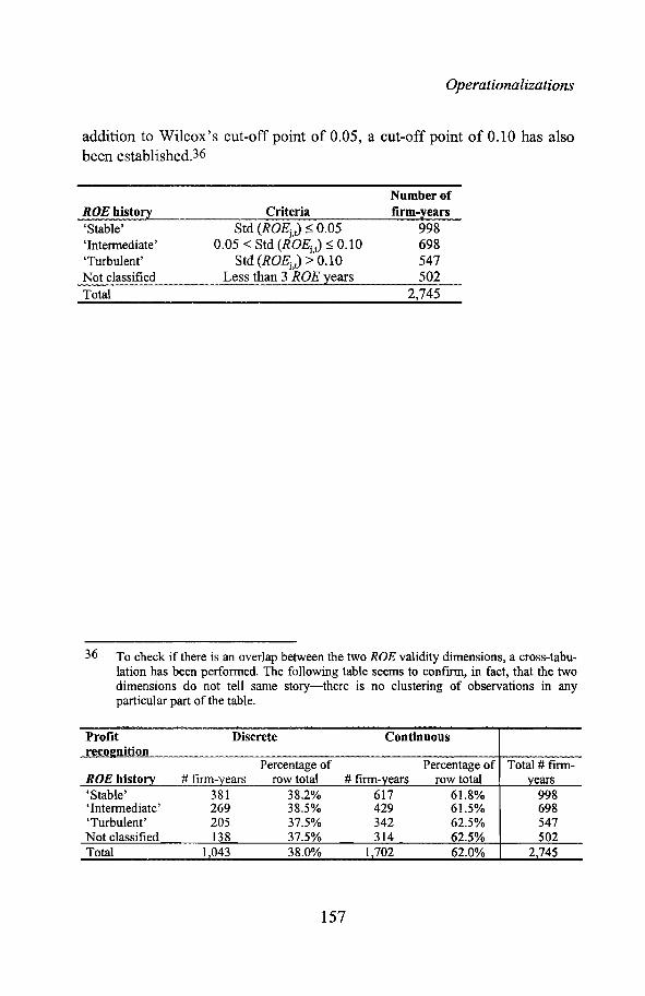
Operationalizations
addition to Wilcox's cut-off point of 0.05, a cut-off point of 0.10 has alsobeen established.36
ROE history'Stable''Intermediate''Turbulent'Not classifiedTotal
CriteriaStd (ROEj,J ~ 0.05
0.05 < Std (ROEj,t) ~ 0.10Std (ROEj,J > 0.10
Less than 3 ROE years
Number offirm-years
998698547502
2,745
36 To check if there is an overlap between the two ROE validity dimensions, a cross-tabulation has been performed. The following table seems to confirm, in fact, that the twodimensions do not tell san1e story-there is no clustering of observations in anyparticular part of the table.
Profit Discrete Continuousrecoa=nition
Percentage of Percentage of Total # firm-ROEhistorv # firm-years row total # firm-years row total years'Stable' 381 38.2% 617 61.8% 998,Intermediate' 269 38.5% 429 61.5% 698'Turbulent' 205 37.5% 342 62.5% 547Not classified 138 37.5% 314 62.5% 502Total 1 043 38.0% 1 702 62.0% 2745
157

Accounting Information and Stock Prices
5.2 Measurement of changes in the economic climate
5.2.1 Inflation rate patternFigure 4.2 illustrated the annual change in the Swedish Consumer PriceIndex and the annualized monthly long-teml interest rate. This informationis supplemented below with a longer-term change in the consumer priceindex to illustrate three aspects of the Swedish inflation rate.
i) "Current inflation rate": The annual change in the Swedish CPI (thedotted and most fluctuating line in thefigure).
ii) "I-listorical inflation rate": The rolling seven-year geometric averagerate of inflation is illustrated by the boldunbroken line.37
iii) "Expected inflation rate": The long-term risk-free interest rate is oftenused as a proxy for the expected futureinflation rate level (the thin unbroken line inthe figure; note that a real risk-freecomponent is usually subtracted in order toassess the expected inflation rate level).
37 Historical inflation rate: ( CPlt )>4 -1CPlt- 7
158

Operationalizations
.. \~~~
'" -'1\. I~\.',
"t' " It \ V I'..V,
" / ~ .'\, .. , ,", • I
, ..~~I-;"""
~, .. ........ ...... , \r-'
~.
V ~~.... ~~
."
.,., ~ ..- ., -- v V~ ~.
,"- \/ , ,'-
., . ,~.
",
/ ~--~.",,' 9- 'I -
",,-~,
1/, .- . "- "~ ,,' :..... ., .. .
r..
L
16%
12%
10%
80/0
6%
4%
2%
0%
""co0)co
('I) It)eX) eX) ""eX)
0)eX)
I· I Year CA - 7 Year ()JI __ Interest rate I
Figure 5.1 The dotted line illustrates the one year change in the Swedish Consumer Price Index (Ll CPI).The bold unbroken line illustrates the annualized 7-year change inthe Swedish CPLThe thin unbroken line illustrates the annualized yield on government bonds. The yield is calculated as the rate ofreturn that equatesthe bondprice with the stream ofremaining cash flows. 38
Relying chiefly on tIle smoother historic inflation rate pattern, a few inflation rate phases can be identified:
PeriodA 1967 - 1972B 1973 - 1980C 1981 - 1984D 1985 - 1993
Inflation rate characteristicsLowRising-low to highHighFalling-high to medium
In Johansson and Ostman (1995, p. 131) it is stated that return on equitymeasures given historic cost accounting can be misleadingly overstated (ascompared to current cost accounting ROE), particularly during the initial
38 Inflation rate figures obtained from the Statistical Yearbooks of Sweden, SCB andFindata.Interest rate figures obtained from the Swedish National Bank-Statistical Yearbooksand Findata.
159

Accounting Information and Stock Prices
period following a significant fall in the rate of inflation. The consequenceswill be reversed if there is a significant increase in the rate of inflation.Basing expected ROE on reported earnings at a time when current ROE isdeemed to poorly reflect performance, can have a detrimental effect on thesignificance of the coefficients in value regressions M.I and M.2.
Johansson and Ostman further maintain that the difference between the twoaccounting methods will be insignificant-even in inflationary periods-ifmonetary assets dominate a company's asset base.39 Thus meaningfulcapital return comparisons can be made between, for example, banks andother companies with non-monetary assets that are only of minorimportance. As the sample of firms in this study, does not include banks,and only relatively few companies with insignificant amounts of nonmonetary assets (such as pure trading and retail con1panies), the inflationary'problematic periods' will be expected to create general performanceinterpretation difficulties for most companies in the sample. However, theseproblems are expected to be especially important for companies that holdlarge amounts of assets with long economic lives, such as firms in the realestate, shipping and paper and pulp industries.
Two extreme san1ples have been chosen to test this hypothesis. Six of the 16industries have been found to include firms that tend to hold large amountsof long-life assets. Five industries have been found to include firms with asmaller relative share of long-life assets.
Industries in which fmus tend to holdlarge amounts of long life-assets• Shipping• Real estate• Mixed real estate and construction• Paper and pulp• Capital-intensive service• Pure investment companies
Industries in which fmns tend to holdsmall amounts of long-life assets• Trading and retail• Engineering• Other production• Other service• Consultants and computer
The median fixed-asset-to-total-asset-ratios in these two groups were 0.67and 0.27 (for 791 and 1,220 firm-year observations respectively).Furthermore, in order to maximize the difference between the two sub-
39 Ibid p. 132.
160
Operationalizations
groups, both the least and the most fixed asset-intensive observations wereexcluded from each group.40 Finally, any firms in the 'limited long-lifesample' with an estimated PMB exceeding 0.50 have been excluded fromthis sample in order to minimize the potential effect of the inflation rate.This criterion reduced this final sub-sample to 644 firm-years.
5.2.2 Changes in the business climateLevel studies (valuation) often refer to the tendency of the regressioncoefficients to be unstable when data are run in cross-section at differentpoints in time (see, e.g. Foster 1986 p. 445). Unstable coefficients may,however, be quite reasonable from an economic point of view. The generalmarket belief concerning future prospects of growth and potential to retain(or eliminate) abnormal performance may be expected to be systematicallydifferent under varying business conditions. A simple factor that attempts tolink next period's expected performance to market value could thus beexpected to vary over time. The regression coefficient PI, in valuationmodel specification M.1 and M.2, is an estimate of such a link, called thegrowth persistence factor (GPF) in this study. To investigate whetller thefluctuations in the business cycle can be an important source for anyinstability in the mentioned regression coefficient in this study, an operationalization of the 'business cycle' is needed.
The overall business cycle descriptions in the "Business Tendency Surveys"published quarterly by the National Institute of Economic Research(Konjunkturinstitutet) consist of a weighted sum of the degree of full capacity utilization and labor shortage in the Swedish industrial sector. Figure 5.2illustrates the level of this index from 1963 to 1994.41 Particular industriesmay have led or lagged in this general pattern. Further precision regardingthis issue could possibly have been reached by using industry-specific business cycle indexes. Such an effort will, however, not be considered.42
40
41
42
After excluding observations when the fixed-asset-to-total-asset-ratio was below andabove 0.40 respectively, the sub-samples consisted of 701 and 992 firm-years, withmedian fixed-asset-to-total-asset-ratios of 0.70 and 0.25 respectively.The level of the index has actually been measured three months after the end of the yearto match the date of the market values being used in this study.It should perhaps be mentioned that another shortcoming of the chosen index relates tothe fact that it describes the Swedish business cycle. Several firms contained in thisstudy operate to a large degree in a global market.
161

Accounting Information and Stock Prices
Utilization of resources in the Swedish Industrial sectorSource: National Institute of Economic Research
70
60
50
40
30
20
10
v~ /1\ /""~
~~ \ / \ / \I \ l Ir\!Ilo.......ol
\./ \ (
1\ /\ I ~j J, I , V \ /, I i\,~ '....-J ~ V"-
o
Figure 5.2 The Swedish industrial resource utilization from 1963 to 1994measured three months after the end ofthe year. The weighted sumof reported incidences of full capacity utilization and labor shortages in the Swedish industrial sector.43
This figure shows that the length of the Swedish industrial business cycleshas varied slightly over the period. Most cycles seem to have lasted four tosix years, except during the 1980s when no deep recession wereexperienced.
Similar phases in the business cycle will be evaluated separately in order toinvestigate if any systematic differences regarding the regressions can beuncovered. All in all, five distinct 'low turning points' seem to haveoccurred between 1967 and 1993, namely 1967, 1971, 1977, 1981, and1992. Similarly four distinct 'high turnings points' have occurred, namely1969, 1973, 1979, and 1988. In the extended boom period of the 1980s, theminor turning points in 1984 and 1986 have thus been viewed to be nondistinct.
43 Source: "Business Tendencies Surveys", Swedish National Institute of EconomicResearch
162

Operationalizations
Value change regression models M.4 and M.5 both rely on the assumptionthat the GPF coefficient is constant over time. If it is shown that the GPFcoefficient tends to vary systematically between different business cyclepl1ases, it should preferably be controlled for in the change specifications.Given the varying lengths of the cycles, such a control can only beperformed for some of the longer value change windows. In appendix P, aclassification of each point in time according to four categories-'Boom','Down', 'Recession' and 'Up'-is shown. The business cycle phases havesubsequently been compared at the beginning and at the end of eachpossible five- and ten-year value change window. Unfortunately, the phasesat the beginning and end of the windows have only coincided in four of the21 five-year value change windows. In the ten-year value change windows,the business cycles have coincided at each end in nine of the 16 possiblewindows. The regression results of these nine windows will be studiedseparately in order to shed some light on the effects of running the proposedregression specifications both with and without control for changes in thebusiness climate.
163

Accounting Information and Stock Prices
5.3 Description of accounting changeThe purpose of this section is to provide detailed descriptions of the gradualchange in, and the expected consequences of, some selected accountingmeasurements and disclosure issues. These issues are open disclosure ofvalue and depreciation according to plan, group consolidation method andaccounting for goodwill, and the accounting method for associatedcompanies.
5.3.1 Open disclosure of value and depreciation according toplan
The transition in disclosure practice is particularly interesting for the firmsin industries that hold relatively large amounts of depreciable assets.44 Todescribe the gradual transition to open disclosure of values according to plan(i.e. open disclosure of the accumulated untaxed reserves related todepreciation for tax purposes in excess of depreciation according to plan),the relative frequency of firms with non-zero values of untaxed reservesrelated to accun1ulated depreciation on machinery and equipment, and shipsand buildings has been calculated.45
Figure 5.3 illustrates i) that approximately only 10% of the firms discloseduntaxed reserves openly in 1967, ii) that a gradual transition to opendisclosure occurred during the period leading up to 1985, and iii) that thestrongest transition took place before 1980.46 One problem in usingFindata's variable number 128 to evaluate the transition of actual disclosurebehavior, is that in some instances Findata has updated the historic data byincluding later disclosed information. With regard to untaxed reserves, thedatabase often includes the new information at least one period before thefirst actual publication. In order to control for this, the actual annual reports
44
4546
A prerequisite for reporting non-zero depreciation, in excess of normal depreciation, isthat the firm holds assets that can be depreciated more aggressively for tax-purposes(and that the firm has generated sufficient profits to have a reason to utilize such anoption). The following industries and companies have thus been excluded: trading andretail, consultants and computer, other service, investment companies, conglomerateand mixed investment companies and real estate.Variable 128 in Findata's database.The transition to open disclosure has been a two stage process for some firms. Firstthese firms provided information in the income statement, and not until one or severalyears later was information given in the balance sheet.
164

Operationalizations
were checked for the years surrounding the first year of disclosure as foundin Findata. The result of this screening can be seen in the figure below (thedark area). Actual open disclosure was apparently published only in lessthan 5% of the firms in 1967.47
Transition to open disclosure of asset valueaccording to plan in the balance sheet
100% ~--r--..,..-,....-..,...-.....,...--,.-~...,....--r-"""'-""""""""""'--""- ......-,.---r-~90% -I--+---+-+-----+---+---I--t---l---+-+--__+___:
800/0 -f----f-----+-+----+-----I---I--+---+----+
70% -f----f------+--+----+-------+----+-+----+--
60% -I--+---+-+---+-----I---I--t----+-
50% -f----+----+--+---+-----I---II----+--
40% -1--+---+--+----+------+---+
300/0 -1---+--+----+-+--_:1::
200/010%
0%
I_ Disclosure in annual statement IIFindata I
Figure 5.3 The relative frequency of firms with non-zero values of untaxedreserves related to accumulated depreciation of machinery andequipment, ships and buildings (variable 128 in Findata). The lightgray area indicates the frequency of firms that in fact did notprovide open disclosure according to a manual check of the firm'sannual reports.
Two ratios have been calculated, in order to quantify the potential effect ofthis accounting issue in terms of book value of equity and return on equity.The unbroken line in figure 5.4 illustrates the after-tax median accumulateddepreciation in excess of depreciation according to plan (only the firms witha non-zero value have been included) divided by book value of equity(including the equity share of untaxed reserves).48 The median ratio ranges
47 Using Findata's variable 128 to estimate disclosure behavior thus overstates the amountof open disclosure firms by approximately 10-20 percentage units for the years leadingup to 1978.
48 VAR 128t .(1- it)
Bt
165

Accounting Information and Stock Prices
between 10 and 20% (for individual companies the variation is muchlarger). Assuming that the firms with non-open disclosure have similarvalues of hidden untaxed reserves, it is obvious that their book values arelargely underestimated. Given the individual variation between firms, theuncertainty cOl1cemil1g a specific firm's underestimation can be expected tobe significant. The broken line illustrates the median absolute after-taxeffect of the reported changes in depreciation in excess of plan relative toopening period equity.49 The level of this ratio is possible to interpret inrelation to ROE. The median value ranged between 2 and 4% in this groupof firms.50 This obviously means that ROE measurement can besignificantly affected (disturbed) for the non-open disclosure firms,provided that the same levels of depreciation in excess of plan also havebeen used among these firms.
Median level and absolute change in accumulated'over depreciation'
25% ......-----------------------...
100/0 +---~---#__------------------I
20% -I--------------I'"-~::__----------I
5% -1-------------------------11
15% -I--------I-~~~---~!!!!!!!!!!!!!!!!I!!!!!!!!!""'-----_I
- ........ .-..•• __ • - ;1 .. ,._. lIlII • __ .
0% .....--;---+--oI__-+-___+_ ~"O+___+____+-oI___+____+_-~_+__ -+__~
...... ex:> 0> 0<0 <.0 <.0 I"0> 0> 0> 0>T'"" T'"" T'"" T'""
---Ace. over depr/B - - - Abs ehange/B(t-1) I
Figure 5.4 The unbroken line illustrates the after-tax median accumulateddepreciation in excess ofplan divided by book value of equity. Thebroken line illustrates the median absolute after-tax effect of thereported depreciation in excess of plan relative to opening periodequity.
49 VAR297 t ·(1-ft )
Bt- 150 This amounts to plus/minus 20 to 40% in comparison to an ROE of 10%. Note also that
the variation between individual firms in particular years has been very large.
166

Operationalizations
The regression models will be run separately on two samples which havebeen formed according to whether or not firms disclose openly.
5.3.2 Group consolidation methods-accounting foracquisitions and treatment of goodwill
To test whether the acquisition activity of a company in general, and thechoice of an accounting group consolidation method in particular, affect theassociation between accounting data and stock prices, the actual acquisitionactivity and accounting methods used must first be identified.
Figure 5.5 illustrates the annual frequency of firms in the sample that havemade a large acquisition.51 The acquisition activity in general was very lowuntil the early 1980s, but particularly intensive acquisition activity followedin 1983, and then from 1986-90. In some of these years, more than 20% ofthe firms made a large acquisition.
51 Large acquisitions have been defined according to one of two criteria:
A .. . GUT GUT GuTDepr GUTWrite-ojfcqUlsltlOnt > 0.25 or "t - "t-1 - "t - ""t > 0.10
Bt BtAcquisition = Variable 343 (investment in shares and acquisitions) in Findata;unfortunately, this variable seems to be unreliably coded in the database.GW = Variable 41 (accumulated goodwill), GW depr. = Variable 212 + 276, GW writeoffs are identified in Rundfelt (1987, 88, 90, 91, 92 and 93). Note that the 'avoided'goodwill in connection with acquisitions paid by issues below market value, is alsoviewed as a goodwill write-off. Rundfelt's surveys focus essentially on the firms on theA lists, implying that some write-off firms among the OTe-listed firms may have beenmissed.
167

Accounting Information and Stock Prices
Annual percentage of firms makinga large acquisition
60°J'o
50°J'o
40°J'o
300/0
200/0
10°J'o
0%....... 0> t: ('t) U") ....... 0>co (0 ....... ....... ....... .......0> 0> 0> 0> 0> (j) 0>T"" T"" T"" T"" T"" T""
Figure 5.5 Annualpercentage ofthe firms in the total sample that make a largeacquisition. (See footnote for definition oflarge.)
The first figure in appendix Q illustrates the transition in chosen consolidation method over the period 1967 to 1993.52 While the pooling (par)method was apparently the most common method in the late 1960s, the ptrrchase method gradually took over during the 1970s. The second figure inappendix Q illustrates the steadily increasing number of firms that reportgoodwill in their financial report (more than 50% of firms in 1993). Thisdevelopment is, of course, a combined result of increased acquisitionactivity and the transition to the purchase method.
The increasing importance of goodwill as an item in the income statement isillustrated in the third figure in appendix Q. The annual (arithmetic) mean ofeach goodwill reporting firm's goodwill depreciation divided by openingbook value of equity has been calculated. The size of this number candirectly be related to the value of ROE. Observe the steady growth from 0 to2.5%. This shows that the reported ROE has been reduced on average by 2.5percentage points for the group of firms that reported goodwill as an asset in
52 Findata has coded different group consolidation methods in variable 336. The relativefrequency has been calculated for groups only.
168

Operationalizations
the early 1990. The last figure in appendix Q ~llustrates the relativefrequency of large goodwill write-offs amongst these firms.53
It is obvious from these graphs that the late 1980s were unique in terms ofsignificant acquisition activity and diverse accounting treatment of theacquired goodwill. How can these phenomena be expected to affect theassociation between the accounting descriptions of these firms and the leveland change of the firms' stock prices?
The reliance on traditional conservative accounting and the purchasemethod for group consolidation means that a company that growsorganically will have different levels of book value of equity, earnings andROE compared with a similar company achieving its growth via severalacquisitions. These differences will be particularly pronounced if thebusiness activity uses either long-lived tangible assets, and/or treats largeexpenditures that could qualify as investments in intangible assets byimmediate expensing. Traditional conservative accounting and organicgrowth create the type of measurement biases discussed at length in thisthesis. It has been argued that for a company that grows at a steady pace andholds a balanced portfolio of its resources, the size of this accountingmeasurement bias will be permanent (in a relative sense). A company that isinvolved in large acquisitions, and uses the purchase method to account forits business activities, will at least temporarily reduce these accountingmeasurement biases as the (new) tangible assets are revalued to currentacquisition cost and acquired intangible assets are capitalized under theheading of goodwill. Thus one effect of the use of this accounting method isthat it obviously 'disturbs' the old reference points for different ratios offinancial performance and financial structure.54 A write-off of acquiredgoodwill can be viewed as a partial reintroduction of the accountingmeasurement bias. This reintroduction, however, may increase thecomparability of the firm's financial ratios to other firms. In the late 1980s,many financial analysts and business magazines such as Affarsvarlden,
53 The firms that have reported a goodwill write-off were identified in Rundfelt (1987, 88,90, 91, 92 and 93).
GwfVrite-ojJA large goodwill write-off has been defined as t > 0.10
Bt- 154 This is evident when comparisons are made with a peer group of non-acquiring firms or
the acquiring firm's own history.
169

Accounting Information and Stock Prices
adjusted the financial numbers in this way for all firms, presumably in orderto gain increased comparability. Which accounting method that is associatedwith the best statistical map between the share price and the accountingnumbers is an empirical question.
The expected effect of acquisition activity and the use of the purchasemethod on the main variables of this study's regression specifications, canquite easily be inferred. The mean market-to-book value premium of firmsthat have recently made large acquisitions is expected to be smaller than themean premium for similar firms that have not made recent acquisitions.
(M JAcq (M JNoAcq
Mean B: - 1 < Mean B: - 1
Similarly, the mean premium is expected to be larger for the firms that haverecently made a large goodwill write-off.
(MJ No Write-off ( M JWrite-off
Mean _t -1 <Mean _t -1Bt Bt
In terms of regression specification M.2, a relatively smaller regression coefficient associated with the PMB (ft2) is expected for the group of acquiringfirms in general, but in particular for the firms that have chosen not to writeoff the acquired goodwill. In terms of the valuation model, as previouslydiscussed in Section 3.3.1, the relatively lower book value of equity that isassociated with a goodwill write-off, will be 'compensated' for by higherfuture earnings and thus higher future ROE ratios. A powerful procedure forpredicting future ROE that takes these accounting differences correctly intoaccount, should ensure that the regression coefficient that is intended tocapture the expected persistence of abnormal performance (PI in regressionspecification M.1 and M.2) remains unaffected. Relying, however, on aperformance prediction procedure that uses the most recent level of ROE asits starting point, the slope coefficient and the regression's explanatorypower cannot be expected to be unaffected. An observation that was quoted
170

Operationalizations
in Section 3.3.155 pointed at the general difficulty involved in understandingand analyzing companies that were continuously restructured via thepurchase and sale of different subsidiaries. The analytical obstacles(generating uncertainty of future performance) that are thus likely to resultfrom acquisition activity in general, combined with the uneven practice ofgoodwill accounting, can be expected to result in PI -coefficients in M.1and M.2, being comparatively low (with low significance), generatingsimultaneously comparatively low R2 of the regression specifications.
In terms of the value change regression specification M.4, similar problemsrelated to the change in expected residual income variable may be expected,resulting in comparatively lower and less significant e2 -coefficients for agroup of acquiring firms. The negative change in book value of equity resulting from a write-off of goodwill can be expected to generate a e1 -coefficient that is negative during the write-off year for a group ofwrite-off firms,assuming that the write-offs are not perceived to represent real reductions invalue.56 The e1 -coefficient should regain its expected normal positive value(close to 1.0) in the years following such a write-off.
Empirical tests of the validity of these assertions will be presented inChapters 7 and 8.
5.3.3 Accounting for associated companiesFigure 5.6 below illustrates both the frequency of firms in the sample thathold shares in associated companies and the relative share of firms that havechosen a particular accounting method.57 The relative drop in associatedconlpany frequency in 1984 is due to the inclusion of OTe firms fronl thatyear and onwards. Holding shares in associated companies is apparently
5556
57
From FAR's Survey of Accounting Practices 1987, p. 14.If the write-off, on the other hand, is perceived to represent a real reduction in value,the regression coefficient should receive a 'normal' value of approximately 1.0.Identification of associated companies has been performed using variable 239(dividends paid from associated companies), variable 234 (profit share after tax in excess of dividend paid, reported in the income statement), and variable 235 (profit shareafter tax in excess of dividend paid, disclosed in the notes). Note that only thefrequency of firms that use the equity method, and given the cost method, the firms thatdisclose profit shares in the notes, have been presented in the figure. An additionalnumber of firms use the cost method without providing profit share information in thenotes.
171

Accounting Information and Stock Prices
much more common among the larger firms on the A-lists. It is noteworthythat some firms used the equity method as early as in 1972, but the mainchange, however, did not begin until the early to mid 1980s. Towards theend of the period studied, the equity method has dominated.
Relative frequency of accounting method forshares held in associated companies
40%
35%
30%
25%
20%
15%
100/0
50/0
0%
1I111~.1I • I rn n Iii ~ I·] rn 1:11
(j)co(j)
EJ Equity rv1ethod • Cost rv1ethod (profit share in notes)
Figure 5.6 Relative frequency offirms in the sample that hold shares in associated companies and the relative share of firms choosing a particular accounting method
Figure 5.7 illustrates the median consequence in tern1S of reported ROErelated to how firms have chosen to account for associated firms. Firmsusing the equity method show a median positive ROE effect between 0 and2% (but a negative median effect during the recession in the early 1990s).The 'hidden' ROE effect (only reported in the notes) related to the costmethod has been quite similar during most of the period (1983 being anexception).
172

Operationalizations
Median profit share in excess of dividends relativeto reported opening book value of equity
5%
40/0
30/0
2°,.'0
10/0
0%
-10/0
"'"co0>~
••....
0>co0>~
••• •I •
---Equity Method - - - Cost Method f
Figure 5. 7 The median profit share in excess ofpaid dividends relative to reported opening book value ofequity for firms reporting according tothe equity method and the cost method.
The size of these median ROE effects implies that investors who base theirvaluation of firms utilizing ROE from published annual statements canreceive different signals of a firm's performance, depending on how theconlpany has chosen to account for their associated companies (if theinformation in the notes is not utilized). As noted previously in Section3.3.1.4, a company switching to the equity method, besides being likely toshow a higher ROE, will also simultaneously show a higher book value ofequity.
In order to investigate if the variables of the regression specifications M.1 toM.S, and/or the resulting regression coefficients are systematically affectedby a switch from the cost method to the equity method, the actual switchyear will first need to be identified. Observations from the switch year, andfrom the two years before and after the switch will then be analyzedseparately.
173

6 REGRESSION VARIABLES
6.1 Calculation of the main variables for thespecified regression models
6.1.1 Market-to-book value premiumsThe dependent variable in M.l and M.2 is the market-to-book value premium, that is the ex-dividend market value divided by the ex-dividend bookvalue, reduced by one. Ex-dividend book value at the end of December eachyear follows the definition in Section 4.2.1.3. Ex-dividend market value ismeasured at the end of March each year to ensure that the market has had achance to incorporate at least the information contained in a press announcement of unaudited annual earnings. Findata's definition of marketvalue has been used,l that is the last bid price (on the most traded type ofshare) n1ultiplied by the total number of shares outstanding at the same date.The market value has been reduced by deducting proposed dividends(typically to be paid in May).2
1 NYC # 143 in Finlis.2 At first, this nleasurenlent procedure appears to be unproblematic. A number of meas
urement problems may, however, be identified. Firstly, a measurement mismatch canoccur if a firm issues new stock during the three-month time span, January to March,creating an 'unfair' comparison between the market and the book value. Using information in Findata, 20 such issues could be identified. To correct this mismatch, the bookvalues of the issues were identified and added to the year-end book values of equity.While this correction was being made, an unfortunate shortcoming in Findata's marketvalue calculation procedure was discovered. If several issues occurred at different timesduring the same year, or if an issue later the same year was followed by a stock dividend, the number of shares outstanding has not been correctly matched with the actualstock prices during the period in between the two issues. This error can lead to a significant overstatement of a firm's market value. Four such instances were identified and,with very helpful assistance from Erik Eklund at Findata, corrected manually.
Another measurement issue relates to the fact that nlany firms have several classes ofshares outstanding. Findata's market value calculation uses the price of the most tradedshare, multiplied by the total number of shares outstanding. A voting power differencebetween so-called A and B shares has sometimes lead to non-trivial price differences onthe two types of shares. According to a study by Rydqvist (1987) the annual cross-

Regression Variables
The calculation of the market-to-book value premium for firmj at time t canthus be written as follows:
[6:1]*M . M . 11 h 1 - D· 11 1~ -1 = j,lYlarc :t+ j,lYlay:t+ -1
B;,t Bj,Dec:t -Dj ,May:t+l + N j ,JantoMarch:t+l
Table 6.1 shows annual market-to-book value statistics for the full sample.
sectional mean of the voting-power premium varied between 1.4% and 6.1 % between1975 and 1985; for individual firms at particular points in time the premium did,however, exceed 40% (see table 5.9 in Rydqvist 1987). The most traded share-type haspredominantly been the lower valued B shares. This means that the Findata calculatedmarket value generally excludes a potential 'voting-power premium'. As the proposedvaluation tnodel utilized in this study does not capture 'voting-power issues' this isprobably also a reasonable choice. An alternative market value calculation would utilizedetailed information of the market price and the number of outstanding shares of eachtype. Given the lack of such data, however, it would involve very cumbersome manualcalculations. Furthermore, one could argue that these calculations of a total marketvalue, as a multiple of the share price times the nUITlber of shares outstanding, in anysense is fictional, not necessarily perfectly representing an expected transaction value ofthe whole stock of shares.
Furthennore, two measurement complications can be noted. If a firm happens to havetraded subscription right certificates outstanding (due to an ongoing new issue) at amarket valuation point in time, the market value of the firm's equity may be underestimated. Underestimation of the market value of equity may also be caused by the existence of other financial instruments with non-trivial value, e.g. convertible debt being'deep into the money' (having a stock price that significantly exceeds the strikingprice). Neither of these problems are, however, expected to have serious effects on thisstudy.
175

Accounting Information and Stock Prices
Table 6.1 Annual statistics for the market-to-book value premium. The lastrow contains the same statistics for all firm-years.
Year196719681969197019711972197319741975197619771978197919801981198219831984198519861987198819891990199119921993Total
Median-0.31-0.05-0.30-0.35-0.09-0.09-0.03-0.16-0.03-0.12-0.29-0.35-0.33-0.14
0.020.681.000.510.671.151.131.641.100.430.00
-0.100.510.38
Mean-0.13
0.09-0.18-0.24
0.130.120.180.040.130.02
-0.15-0.08-0.06
0.180.451.131.450.800.961.671.732.331.780.770.250.130.810.76
Std0.480.550.350.390.730.650.690.640.610.600.570.760.780.931.181.341.341.101.111.912.222.652.291.401.160.920.971.60
N
3939424370727679788386888991929596
152161164169168166151129119108
2,745
In figure 6.1 the frequency distribution of all the calculated market-to-bookvalue premiums is shown (2,745 firm-year observations). The bulk of observations clusters around a premium between -0.5 and 1.0. The distribution ofobservations obviously does not follow the normal distribution. Observations below -1.00 are not possible, whereas a number of quite extreme positive observations are present (including 10 firm-year observations outsidethe boundaries of the graph).3
3 The maximum market-to-book value premiunl observation is 20.4 in 1989, for a realestate company called Lodet. The same company has three more observations exceeding 10. To check for the presence of outliers caused by errors in the market-to-
176

Regression Variables
400
Std. [£y= 1,00~=,8
~E3l::~~:i.J....,..c:;::::"---'=;:::a-- __----J N=2745,00
I'v1arket-to-book - 1
Figure 6.1 Frequency distribution ofcalculated market-to-book value premiumfor all firm-years. Ten observations with premiums exceeding 10 al·enot included in the graph.
6.1.2 Prediction ofROE for the next period-in practiceIn Section 4.2.3.3 different potential prediction procedures of ROE for thenext period were discussed. In this section, the S-shaped model (P3) will beevaluated on the data presented in Section 4.2.1.5. The estimation of the parameters for the S-shaped model is performed in two (iterative) steps. Thevalue of a2 that maximizes the explanatory power of the following linearfunction is searched for:4
where
book value calculation, a firm specific check was performed. The size of all the premiums was ranked on individual firm level. Firm-years when the most extreme premium(s) deviated significantly from the second (or third) most extreme premium werethen closely analyzed. Extreme observations from approximately 20 firms were identified. None of these observations was found to be incorrect.
4 See Freeman and Tse (1992) for further discussion of this two-stage approach.
177
7 Runsten

Accounting Information and Stock Prices
[6:3] x .t == arctan[(ROE . t - P.t - f .) .a2]], ],],]
The regression has been specified without an intercept to be consistent withprediction model P3.5
The estimation of the market's cost of equity capital (Pt) follows the presentation in Section 4.2.2. All the firms in the sample have an accountingyear ending in December. Investors are assumed to be aware of the firms'previous year's accounting performance at the end of March (the followingyear)-eon1municated via a press release of unaudited annual earnings or anearly annual report. The end of March has also been used as the measurement date of market value in the regression specifications M.1 to M.S. Consistent with these cl10ices, Pj,t has also been measured at the end of March.This means that the long term government bond rate and Findata's 48month firm specific market beta have been measured at this date every year.In order not to lose observations, beta has been assumed to be equal to 1.0during the first four years (= 48 months), after the firm has been listed. Yjvaries between industries, but has been set constant over time.
All ROE observations from 1967 until 1993 have been used in a pooledtime-series and cross-sectional regression. Actual ROE (adjusted for the'hurdle rate') for 1967 has thus been compared to the similarly adjustedactual ROE for 1968; similarly, 1968 has been compared to 1969 and so onuntil 1993. To assess the robustness of the regression results, the sample hasbeen divided into three separate time periods, in two ROE history groups,and two profit recognition groups.6 The following linear regression hasfinally also been estimated on the same data as a benchmark.
5 The same regression specification has also been run including an intercept. The inclusion of an intercept yielded generally marginally higher R2,s, and estimated interceptsclose to zero.
6 The classification of firms according to ROE history and profit recognition has beendiscussed in Section 4.3.1.4, under the heading ROE validity.
178

Regression Variables
Note that [6:4] is equal to [6:2] when a2 approaches zero. This means thatthe S-shaped regression will always generate explanatory power that is atleast as high as the linear regression. If the S-shaped model dominates thelinear model, the degree of domination can be assessed in terms of the differences in the regression's R2. Regression results are presented in table6.2.7
Table 6.2 The results of the ordinary least square regressions of [6:2] and[6:4]. The first column shows the period studied. The follo~ng
columns include the regression coefficients of the two models. Thenumber of observations in each regression is marked n. The lastcolumn indicates alterations from the full-sample-all-years specification.
S-shaped function Linear function
Period A
R2 A
R2 n Sampleal a2 at ·a2 hI1967 ~ 93 0.25** 3.56 0.90 0.23 0.50** 0.14 2,490 Full sample
1961 ~ 77 0.69** 1.16 0.80 0.39 0.76** 0.38 617 Early
1977 ~ 85 0.25** 3.52 0.89 0.32 0.51 ** 0.18 761 Middle
1985 ~ 93 0.23** 4.05 0.94 0.17 0.46** 0.10 1,112 Late
ROE ValidityROE History
1967 ~ 93 ~oo ~O 0.94 0.35 0.94** 0.35 934 'Stable'ROE History
1967 ~ 93 0.30** 3.18 0.96 0.28 0.56** 0.19 1,057 'Interm. or Turbu.'Profit recognition
1967 ~ 93 0.23** 3.87 0.87 0.21 0.42** 0.12 1,545 'Continuous'Profit recognition
1967 ~ 93 0.29** 3.21 0.94 0.26 0.67** 0.21 945 'Discrete'
A one-sided test for slope coefficients.* significant at 0.01< a < 0.05** significant at a < 0.01
7 The regressions have been run using the statistics and spread sheet functions in EXCEL7.0. a2 has initially been set as an arbitrary constant. Xj t is calculated in one column ofcells using a2, actual ROEj t, estimated Pj t and Yj, mid the arctan transformation according to [4:2]. ROE} t+1 minus Pj t and ~ is calculated in a parallel column of cells.[4:3] is then run as an ordinary least square regression (OLS). Using the iterative'problem solver function' in EXCEL, the level of a2 that maximizes the regression's R2has been located.
179

Accounting Information and Stock Prices
The first column shows the period studied. The following columns includethe regression coefficients of the two models. The product of al and a2 isalso presented, as it indicates the slope of the regression close to the origin.The product is thus comparable to the slope coefficient of the linear regression (hI)' The explanatory power (R2) of both regressions for each alterationis presented in separate columns. The number of observations in each regression is marked n. The last column indicates alterations from the fullsample-alI-years specification.
The regression results support the hypothesis of a general mean reversiontendency in the development of ROE. Both hI and ara2 are less than one.However, the linear functiol1 indicates a rather strong mean reversion tendency (hI == 0.50 for the full sample), whereas the S-shaped function indicates weak mean reversion for normal ROE (al·a2 = 0.90) and strongermean reversion for more extreme ROE (al in the full sample is 0.25). Fittinga straight line to data with a number, extreme observations with a particularly strong mean reversion will tend to give a low slope coefficient. Furthermore, the explanatory power of the S-shaped function is almost twice ashigh in comparison to the linear function (23% versus 14%).
Separating the data in three sub-periods, an early period (1967-77), a middleperiod (1977-1985), and a late period (1985-93), further support the dominal1ce of the S-shaped function.
Separating the data according to historical stability in ROE generated interesting results. For the sub-sample of firms with a 'stable' ROE history(std(ROE S .05)), the relationship is best described by the linear function,but with a slope coefficient of 0.94. This slope coefficient is similar to theclose-to-the-origin slope coefficients of the S-shaped function achievedwhen the more turbulent firms were included in the regression. For the subsample of firms \vith an 'intermediate or turbulent' ROE-history (std(ROE >.05)), the relationship is best described by the S-shaped function. Theexplanatory power is 28% versus 19%, and the slope coefficient close-tothe-origin of the S-shaped function (al·a2) is much higher than slope coefficient of the linear function (0.94 versus 0.56). These results further supportthe hypothesis of a mild mean reversion tendency at 'normal' levels of ROE,but a stronger mean reversion tendency at more extreme levels.
180

Regression Variables
Splitting the sample according to the profit recognition categories'continuous' versus 'discrete', the S-shaped function performs best for bothcategories.8
In summary, the regression results support the hypothesis of one period persistence in ROE, with a small mean reversion tendency in ROE for nonextreme levels and a larger mean reversion tendency for extreme levels.Hence, the use of the S-shaped prediction model (P3), rather than the linearmodels PI or P2, is supported.
The choice of 'suitable' levels of at and a2 could follow two strategies:
1. Use different estimated coefficients for different years.2. Estimate al and a2 once, and use these coefficients for the whole period
of study.
To prevent the prediction procedure from becoming too complicated, thesame coefficients for all periods have been used. The estimated slope coefficients of the full sample have been used, hence the prediction function ofnext periods ROE can finally be written as in [6:5]:
8 Several other re-runs of the regressions were done to check how sensitive the regressionresults are to the use of a firm-specific risk measure (f3i t) (as opposed to no risk differentiation between firms (beta = l)), the inclusion of a firm-specific expected permanentmeasurement bias (r j), and the choice of the risk premium (5% vs. 3% and 0%). Theresults are summarized in the table below. As can be seen, the regression results varyvery modestly between the different specifications.
S-shaped function Linear functionPeriod A al ·a2 R2 ;;1 R2 n Alterationsa, a?
1967 ~93 0.25** 3.56 0.90 0.23 0.50** 0.14 2,490 Base case1967 ~93 0.26** 3.48 0.89 0.22 0.50** 0.14 2,490 Pj,t = 11967 ~93 0.24** 3.68 0.88 0.24 0.48** 0.17 2,490 Yj =01967 ~93 0.24** 3.63 0.86 0.24 0.47** 0.16 2,490 Risk premo = 3 %1967 ~93 0.22** 3.86 0.83 0.24 0.43** 0.18 2490 Risk nrem. = 0 %
181
Accounting Information and Stock Prices
6.1.3 Expected residual returnA key independent variable in regression model M.l and M.2 is the expected residual return. This variable was specified in Chapter 2 (note thatYj,t is equal to zero in M.l):
[2:35]
A prediction model for the expected return on equity for the next period wasspecified in the previous section:
Combining these two functions achieves:
[6:6]0.25 . arctan[(ROE . t - P.t - f .) · 3.56]
E [Ri? ]- ], ], ]t it+l - 1 A
+ Pi,t
In figure 6.2 below, the frequency distribution of all the calculated expectedresidual return estimates is showed (2,745 firm-year observations).9 A normal distribution curve is also drawn in the figure, based on the mean andstandard deviation of the observations (-3.4% and 8.5%, respectively). Theshape of the actual distribution indicates a slight leptokurtic pattern, that is,too many observations close to the mean and tails that are 'too fat' compared to the normal distribution. Note that the negative mean means that thegenerated average ROE has not reached the estimated hurdle rate (the costof equity capital plus the return measurement bias); this can partly be explained by the chosen ROE definition that excludes the on average positiveextraordinary items. 10
9
10
A useful side-effect of the prediction procedure is that it also serves as a truncation rule.The potential problem with outliers is thus alleviated.In order to check for sensitivity [6:6] was re-calculated without firm-specific risk differentiation (beta = 1), without the inclusion of a firm-specific expected permanent measurement bias (Yj = 0) and with ROE including extraordinary items (ROEC). The correla-
182

Regression Variables
500
400
300
200
~100c:
Std. Dev =.08Q):::s
Mean =-.034C"~
0 N =2745.00u..
E[RR]
Figure 6.2 Frequency distribution ofcalculated expected residual return for allfirm-years.
tion coefficients amounting to 0.99 (see table below) imply that the attempted 'finetuning' related to risk-differentiation and the inclusion of an annual measurement biasneither adds nor distorts the discriminating ability of the performance measure. However, the choice of earnings definition has a more significant impact.
The pairwise correlation coefficients for all firm-year observations estimated using[6:6] and different specifications.
Base-case Pj,t = 1 Yj =0 ROEC Mean Standard- Ndeviation
Base-case 1.0 0.994 0.997 0.819 -3.4% 8.5% 2,745f3},t = 1 1.0 0.991 0.815 -3.6% 8.4% 2,745Yj =0 1.0 0.817 -2.3% 8.6% 2,745ROEC 1.0 -1.7% 9.7% 2,745
183

Accounting Information and Stock Prices
6.1.4 Calculation of the dependent and independent variablesfor the change specifications
The same calculations as described for the level specification above have ingeneral been used for all the individual components in the change specifications: market value and book value of equity, earnings, ROE, cost of equitycapital, expected residual return, and PMB. The calculations are, however,perfomled on a per share basis. The estimated number of shares outstandingadjusted for stock splits and stock dividends (NYC # 19 in Findata) has beenused. 11
6.1.4.1 The change in market value
The variable to explain in regression specifications M.3, M.4 and M.5 is thechange in the share price for periods ranging between one and ten years.Value change has been measured from the last trading day in March of acertain year until the last trading day at the end of March 1, 2, 5 and 10years later. Price has been measured as the ex-dividend market valuedivided by the number of shares outstanding. Figure 6.3 shows thedistribution of annual price changes for the whole sanlple, (Pj,t denotes priceper share). As can be seen from the figure, there are a few extreme positiveobservations-with an annual price change exceeding 150%. These fewextreme observations may have a large impact on ordinary least squareregressions, and for this reason the regressions will also be run using areduced sample.
11 Findata's adjustment procedure follows the recommendation by the Swedish Association for Financial Analysts (SFF). Manual corrections have been made, when issuesbetween January and March have occurred.
184

Regression Variables
300 ..------------------.....
200
100
~c:Q)::JC"~
U. 0
1-year change in price
Figure 6.3 Frequency distribution ofannual price changes for all firm-years.
Table 6.3 provides summary data for the period lengtlls studied. Note thatthe number of extreme firm-year observations (more than two standard deviations from the mean) comprise less than 3% of the data for all time periods.
Table 6.3 Summary data on periodical price change for the full sample.
Pj,t+k - Pj,tMedian Std Maximum Minimum N
Pj,tMean
1 year 0.12 0.19 0.51 5.79 -0.93 2,4832 years 0.23 0.41 0.90 11.43 -0.99 2,2235 years 0.71 1.35 2.20 28.96 -0.99 1,53910 years 3.15 5.01 6.91 103.88 -0.79 801
6.1.4.2 The change in book value
The change in ex-dividend book value per share (bt), divided by openingshare price, has been calculated for all observations. Figure 6.4 illustratesthe distribution of the variable for the whole sample, and shows a large concentration of observations close to the nlean. It is also interesting to notethat the mean change in book value of equity is approximately half the size
185

Accounting Information and Stock Prices
of the mean change in the share price. This appears to be the case for bothshort and long periods. There are also a number of extreme observations(some of these are outside the boundaries of the histogram). Minimum andmaximum observations along with other summary statistics for all the periods are provided in table 6.4.
700 .--.-------------------
600
500
400
300
200
'7 ~'>1.5', ~e5'0, ~~e5', '00,°00 ,
~..9e5' ~~ ~Ye5' ~~O00e5'
.~1.5' °60 .,>e5'
\j)0 '.e5'e5' '.<90
1-year change in book value per share/opening price
Figure 6.4 Frequency distribution ofannual change in book value ofequity pershare divided by opening periodprice for the full sample.
Table 6.4 Summary data on change in book value of equity per share divided by opening period price for the full sample.
bj,t+k -bj,tMedian Mean Std Maximum Minimum N
Ij,t
1 year 0.06 0.06 0.27 2.03 -3.29 2,4832 years 0.14 0.16 0.34 2.53 -2.67 2,2235 years 0.51 0.66 0.73 7.09 -2.99 1,53910 years 1.84 2.41 2.71 30.91 -3.48 801
186

Regression Variables
6.1.4.3 The change in expected residual income
Firm-specific estimates of expected residual return, calculated as illustratedin Section 6.1.3, have been multiplied by the book value of equity per shareto gain an estimate of expected annual residual income. The change(difference) in expected residual income per share between two points intime has then been divided by the opening share price.l2 The sameprocedure has been used for the 2, 5 and 10 year change calculations. Figure6.5 illustrates the distribution of annual change in residual income for thewhole sample. As can be seen fronl the figure, a large concentration ofobservations are found close to the mean. Furthermore, the mean is close tozero, tIle distribution is symmetric (but not normally distributed), and theoccurrence of extreme cases is rather small (about 2 percent of theobservations). The variable has been constructed to measure changes in theability to create value. In a 'good news' versus 'bad news' sense, in theterminology of Ball and Brown, a zero mean of this variable indicates thatthe average signal contains 'no news'.
600 ...------------------------,
500
400
300
100
200
~c:CD:::sC"~U.
~6'o, ~~,
~6d> ~9'<9
~9'o \?o ~~o ~ J'o ~q, .~ '~o '\ib '9'0 .~
'~a<9 '~~<9 ~ {s» '~O<9 '.~ "? ".~ \~ ".~ ".~
1 year change in Rl/opening price
Figure 6.5 Frequency distribution of the annual change in expected residualincome per share divided by opening period price for the full sample.
12 See Section 2.5.2 for more details regarding this specification.
187

Accounting Information and Stock Prices
Table 6.5 provides summary data for all the periods studied. Note that themean change is negative for the longer periods, especially for the 10 yearperiod. This is not surprising, however, given the design of the variable andan on average estimated negative residual return (see Section 6.1.3) combined with growth in equity (which especially over a 10-year period n1ay bevery large, see table 6.4 for summary data).
Table 6.5 Summary data on change in expected residual income per sharedivided by opening period price for the full sample.
Median Mean Std Maximum Minimum N
0.00 0.00 0.09 0.71 -0.60 2,4830.00 0.00 0.11 1.46 -0.63 2,223
-0.02 -0.01 0.17 2.44 -0.77 1,539-0.09 -0.07 0.52 9.45 -2.62 801
MUp
1 year2 years5 years10 years
6.1.4.4 The change in book value times the PMBIn regression specification M.5, a multiple of the change in book value ofequity and the estimated level of the industry- (firm-) specific permanentmeasurement bias (PMB) has been added as an explanatory variable. I3 Thecalculation of this variable is straightforward, given the calculated change inbook value and the estimated PMBs. Given no expected measurement biasthis variable amounts, of course, to zero. Figure 6.6 illustrates the distribution of annual book value changes multiplied by the estimated PMBs for thefull sample.
13 ~ee Section 2.5.2 for more details regarding this specification.
188

Regression Variables
600 ....------------------------.
500
400
300
200
~r:: 100Q):;]C"
~U.
~6'o, ~vO ~J>O ~~O, ~ 70 ~OO .70 ,
~Vc9 '~J>c9 '~~c9 ~ 7c9
'~0c9 '.~ .?·~o ''''0 '170 ..
'.~~ ".~ .~
1-year change in book value of equity *PMB/opening price
Figure 6.6 Frequency distribution ofannual change in book value ofequity pershare times the estimated industry-specific PMB divided by openingperiod price for the full sample.
189


Part III
EMPIRICAL RESULTS
7 The Level Approach8 The Change Approach9 Summary and Concluding Remarks


7 EMPIRICAL RESULTS: THE LEVEL
ApPROACH
The level specifications, M.1 and M.2, and the change specifications, M.3 toM.5, have all been modeled as linear equations and they will be evaluatedusing an ordinary least square (OLS) approach. This statistical regressionapproach has been commonplace in previous market-based accoWlting research (MBAR). The relative level of the explanatory power (R2) of linearregressions has often been used as a key metric in MBAR (see e.g. the oftenquoted review article by Lev [1990]). Furthermore, the size and significance(relative t-values) of the so-called 'earnings response coefficients' (ERG)have been widely discussed in most published MBAR. This study will relyon the same statistical method. It should, however, be emphasized that thisstatistical approach is rather sensitive to the properties of the data utilized. 1
As a first step in Section 7.1, the simple bi-variate regression model M.l hasbeen evaluated. This model specification is consistent with an accountingprocedure with no accoul1ting measurement bias. Regressions have been runboth annually in cross-section and in pooled time series and cross-section,first for the full sample of firms and subsequently for different sub-samples.The sub-samples have been based on the previously presented firm characteristics. In Section 7.2 the same regressions have been repeated, using regression specification M.2 including the permanent measurement bias.Sections 7.3 and 7.4 present regression results evaluating different changesin the economic climate and some accounting issues.
See appendix R for a discussion of some critical aspects related to this study. For ageneral discussion, see an econometrics text book, such as Gujarati (1988) or Greene(1993).

Accounting Information and Stock Prices
7.1
M.l
Regression model M.l
7.1.1 The full sample
In table 7.1 the annual regression results for the full san1ple of firms arepresented. This presentation format will be used in several tables that follow. The years in the table refer to the book value year-end. As explainedearlier, the market value is measured three months into the following year.The last two rows contain the mean of all the annual regressions and theregression results for a pooled regression of all firm-year observations, respectively. t-statistics are provided in the parenthesis next to each coefficient estimate. These t-statistics give an indication of the precision of thecoefficient estimate. As the 'true' limit for significance judgment is uncertain, statements of significance must be judged cautiously. Nevertheless, thedegree of significance given conventional limits for the 5 percent and 1 percent levels are provided, and distinguished by one (*) or two asterisks (**).R2 denotes the explanatory power of the independent variable, that is thevariation in the market-to-book value premium that can be explained by theexpected residual return variable. The number of observations in each regression is provided in the last column.
194

Table 7.1
Empirical Results: The Level Approach
Annual regression results for regression specification M.1 usingthe full sample.
YEAR Ex PI R2 n
1967 0.13 (1.7) 7.23 (5.4)** 44.3% 391968 0.21 (2.9)** 6.72 (5.2)** 42.3% 391969 -0.14 (-3.1)** 3.98 (5.1)** 39.4% 421970 -0.10 (-1.7) 5.54 (4.4)** 32.1% 431971 0.46 (6.3)** 12.54 (8.4)** 51.1% 701972 0.21 (3.0)** 5.66 (4.4)** 21.4% 721973 0.12 (1.5) 3.80 (2.9)** 10.0% 761974 0.04 (0.5) 0.27 (0.3) 0.1% 791975 0.19 (3.1)** 4.22 (4.6)** 22.0% 781976 0.18 (3.1)** 5.01 (7.0)** 37.8% 831977 0.07 (1.0) 3.49 (5.0)** 23.1% 861978 0.15 (1.7) 3.96 (4.3)** 17.7% 881979 0.11 (1.3) 4.36 (4.2)** 16.8% 891980 0.44 (4.3)** 5.75 (4.8)** 20.3% 911981 0.77 (6.8)** 8.87 (6.5)** 32.0% 921982 1.41 (11.2)** 8.24 (6.1)** 28.3% 951983 1.54 (11.6)** 4.65 (3.2)** 9.9% 961984 0.84 (9.9)** 4.87 (4.5)** 11.8% 1521985 1.00 (11.9)** 4.31 (3.8)** 8.1% 1611986 1.69 (11.4)** 3.11 (1.8)* 2.0% 1641987 1.74 (10.2)** 2.43 (1.1) 0.7% 1691988 2.36 (11.3)** -1.93 (-0.7) 0.3% 1681989 1.76 (9.9)** -2.66 (-1.3) 1.1% 1661990 0.80 (6.8)** 1.20 (1.0) 0.7% 1511991 0.63 (5.6)** 5.72 (5.8)** 21.2% 1291992 0.45 (4.2)** 3.35 (4.3)** 13.9% 1191993 0.88 (9.8)** 2.74 (4.0)** 13.2% 108Mean 0.66 4.35 19.3% 102
Pooled 0.86 (28.1)** 4.40 (12.8)** 5.6% 2..745
t-statistics in parenthesis, a two-sided test is used for intercepts and a one-sided test for theslope coefficients.
* Significant at 0.01 ~ a. ~ 0.05** Significant at a. ~ 0.01
The slope coefficient (/31) is positive and significant at the 1 percent levelfor 21 of the 27 annual regressions. /31 varies between 2.74 and 12.54 forthese years. /31 is non-significant in the regression of 1974 and in a series ofyears between 1987 and 1990. The overall mean of PI' for all annual regres-
195

Accounting Information and Stock Prices
sions is 4.35, which in tum is very similar to the pooled regression coefficient (4.40).
The slope coefficient can be interpreted as an estimate of the averagegrowth persistence factor (GPF). Recall that the GPF in valuationspecification [2: 16] was constructed from the components i) expectedpersistence in abnormal performance (with a 'fading-factor' (A) and lengthof time (1) as sub-components), ii) expected growth (G=l+g), and iii) thecost of equity capital (P). Formally the GPF was specified as follows inChapter 2:
[2:36] GPF=
1_(0.2)Tl+p
1_(0.2)l+p
Table 2.3a-e il1 Chapter 2 provides an illustration of how different combinations of these components together generate different levels of the factor.Table 2.3c, for example, shows that a ten-year period with abnormal performance that gradually fades away with a fading speed of 0.80, combinedwith an annual growth rate between 10 to 15% generates a GPFin the rangebetween 4.0 and 4.5 (given a cost of equity of 15%). The same level of GPFis also consistent with 5 years of a permanent (2 = 1) abnormal ROE leveland an annual growth rate amounting to between 5 and 10%.
The intercept (a ) is oftel1 close to zero until 1980; from this year onwardsa is significantly positive in all regressions. On average a amounts to 0.66.
The average explanatory power of all the annual regressions is 19.3%. Astriking result is that the expected residual return has no or very limited explanatory power during the period 1983 to 1990. This is also the case for1973 and 'especially' 1974.
The pooled regression gives strongly significant regression coefficients a =0.86 and PI = 4.40 (with t-statistics = 28.1 and 12.8 respectively); the explanatory power is, however, as low as 5.6%.
196

Empirical Results: The Level Approach
The unstable and partly weak results in table 7.1 are not unexpected. A heterogeneous group of firms is studied over a period of time that is characterized by important changes in accounting practice and economic climate. Theuse of a simple regression spe~ification and a crude approach for estimatingthe expected next period return (based on previous year's performance) areother influential factors. The relative importance of each of these factorswill be elaborated on in the following sections.
7.1.2 Sub-sample regressions controlling for different expectedvalidity of historical ROE and GPF levels
The con1plete results of all performed regressions will not be presented.However, table 7.2 contains the results of several pooled cross-sectional andtime-series regressions and table 7.3 contains the mean of repeated annualcross-sectional regressions of some selected sub-samples.
Two dimensions of the validity of historical ROE as a base for prediction ofnext period perfoffi1ance were discussed and operationalized in Section5.1.4. One dimension related to whether profit recognition could be expected to occur continuously or to follow a more discrete pattern. The otherdimension related to tl1e stability of the firm's profitability.
Pooled regressions have first been estimated for individual sub-samples.Subsequently, three pooled regressions have been estimated controlling forthe first ROE validity criterion. Three pooled regressions have then beenestimated with the data divided according to the estimated GPF criteria.2
Finally a 'homogenized sub-sample' has been specified. This sub-sampleconsists of firms from industries with a continuous profit recognition, firmyears with a non-turbulent ROE history, and firm-years with medium expected GPF. The purpose of using this sub-sample is to establish if theelimination of firm-years that are expected to be most extreme, in the specified a priori dimensions, improves the explanatory power of the regressionspecification and if it increases the stability of the regression coefficients.
2 The operationalization and estimation of different subgroups related to the expectedGPFwere performed in Section 5.1.3.
197

Accounting Information and Stock Prices
Should this be the case, it indicates the relevance of the dimensions andsuggests that this homogenized sample may be a better base-sample forsome of the later regressions testing accounting change issues. The annualregression results given this last sample specification are provided in table7.4.
Table 7.2 Summarized pooled regressions for different sub-samples of firmsusing regression model M.I.
Sample characteristics a PI R2 nFull sample 0.86 (28.1)** 4.40 (12.8)** 5.6% 2,745
Profit rec. = Continuous 0.65 (22.8)** 5.38 (16.2)** 13.4% 1,702Profit rec. = Discrete 1.22 (18.3)** 3.91 (S.5)** 2.9% 1,043
ROE hist. = Stable 0.80 (14.3)** 5.76 (S.4)** 2.8% 998!ROE hist. = Intermediate 0.96 (14.6)** 5.74 (6.8)** 6.2% 698lROE hist. = Turbulent 0.80 (12.S)** 3.12 (7.0)** 8.2% 547
Profit rec. = Continuous &ROE hist. = Stable 0.55 (15.4)** 10.90 (14.S)** 25.5% 617ROE hist. = Intermediate 0.78 (11.S)** 7.86 (8.7)** 15.1% 429ROE hist. = Turbulent 0.68 (9.2)** 2.64 (4.9)** 6.7% 342
E[GPF] = Low 0.90 (7.3)** 3.47 (S.l)** 6.6% 367E[GPF] = Medium 0.85 (2S.2)** 5.71 (10.4)** 4.6% 2,246E[GPF] = High 0.42 (2.4)** 9.62 (S.S)** 18.9% 132
Homogenized sample 0.62 (16.8)** 10.42 (14.7)** 18.8% 941
t-statistics in parenthesis, a two-sided test is used for intercepts and a one-sided test for theslope coefficients.
* Significant at 0.01 :::; a ~ 0.05** Significant at a ~ 0.01
198
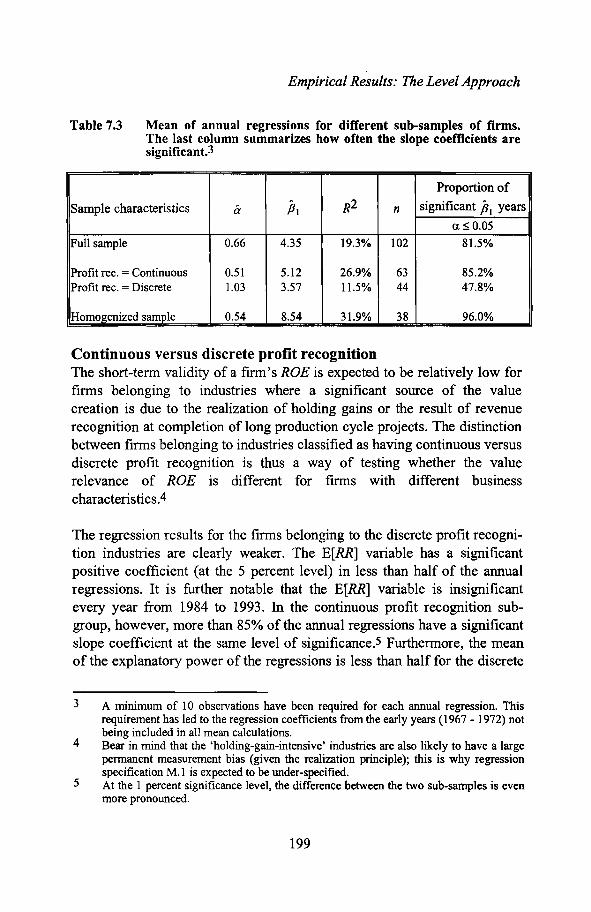
Table 7.3
Empirical Results: The Level Approach
Mean of annual regressions for different sub-samples of firms.The last column summarizes how often the slope coefficients aresignificant.3
Proportion of
Sample characteristics a PI R2 n significant PI years
a~0.05
Full sample 0.66 4.35 19.3% 102 81.5%
Profit rec. = Continuous 0.51 5.12 26.9% 63 85.2%Profit rec. = Discrete 1.03 3.57 11.5% 44 47.8%
Homogenized sample 0.54 8.54 31.9% 38 96.0%
Continuous versus discrete profit recognitionThe short-term validity of a firm's ROE is expected to be relatively low forfirms belonging to industries where a significant source of the valuecreation is due to the realization of holding gains or the result of revenuerecognition at completion of long production cycle projects. The distinctionbetween firms belonging to industries classified as having continuous versusdiscrete profit recognition is thus a way of testing whether the valuerelevance of ROE is different for firms with different businesscharacteristics.4
The regression results for the firms belonging to the discrete profit recognition industries are clearly weaker. The E[RR] variable has a significantpositive coefficient (at the 5 percent level) in less than half of the annualregressions. It is further notable that the E[RR] variable is insignificantevery year from 1984 to 1993. In the continuous profit recognition subgroup, however, more than 85% of the annual regressions have a significantslope coefficient at the same level of significance.5 Furthermore, the meanof the explanatory power of the regressions is less than half for the discrete
3
4
5
A mininlunl of 10 observations have been required for each annual regression. Thisrequirement has led to the regression coefficients from the early years (1967 - 1972) notbeing included in all mean calculations.Bear in mind that the 'holding-gain-intensive' industries are also likely to have a largepermanent measurement bias (given the realization principle); this is why regressionspecification M.I is expected to be under-specified.At the I percent significance level, the difference between the two sub-samples is evenmore pronounced.
199

Accounting Information and Stock Prices
profit recognition subgroup of firms, as compared to the continuous subgroup (11.5% vs. 26.9%). In the pooled regressions this pattern is even morepronounced (2.9% vs. 13.4%).
Relative stability in ROE historyThe rationale behind dividing the firm-year observations into three subgroups depending on the relative stability of the most recent (five) years'reported ROE, relates to the estimation procedure of the expected next yearROE. A stable history is assumed to be associated with more reliable predictions.
It is notable that all three subgroups of firm-years show low statistical association, with similar levels of the slope coefficient. If any trend regardingthe level ofR2 can be traced, it is in the opposite direction as compared to apriori expectations (slightly higher R2 the more unstable the ROE history).Given the results discussed in the previous paragraph, one could argue that astable ROE track-record may be the result of a chosen smooth recognitionpolicy of profits in 'holding-gain-intensive' firms, rather than actual stablevalue creation. This argument is supported by the regressions controlling fordifferent profit recognition characteristics. Results are reported for thepooled sample in table 7.2. The R2 is 25.5%, 15.1% and 6.7% for the stable,intermediate, and the turbulent ROE history groups respectively, when onlycontinuous profit recognition industries are included in the regressions.
Another interesting result from the regressions dividing the sample according to historical ROE stability, is the size of the slope coefficients. Morestable historical returns seenl to be associated with larger GPFs (PI = 10.9,7.9 and 2.6 for the stable, intermediate, and the turbulent ROE historygroups respectively, when only continuous profit recognition industries areincluded in the regressions). This result is consistent with stating that investors expect higher persistence in abnormal performance (T being largerand/or the fading factor (A) being larger (closer to one)) for firms that haveshown a higher stability in past ROE values.
Expected GPFIn Sectiol1 5.1.3 the sample of firms was divided into three categories withregard to the a priori expected level of the GPF. A group of high expectedGPF firm-years was identified using the combined selection criteria of high
200

Empirical Results: The Level Approach
historic growth and a track-record of positive residu£.l return. Low expectedGPF firms-years were similarly selected as firm-years when the most recentROEs were either extremely high or low. These selection criteria did notprovide a sufficient number of observations in the extreme groups to makeannual regressions meaningful. The results of three pooled regressions are,however, provided in table 7.2.
The level of the estimated GPF coefficients (PI = 3.5, 5.7 and 9.6 for thelow, medium, and the high GPF groups respectively) supports the validityof the classificatiol1. Note, however, that the exclusion of extreme expectedGPF firm-years actually slightly reduces the overall explanatory power ascompared to the full sample (R2 = 4.6% versus 5.6%). On the other hand,the two subgroups classified as having extreme GPF firm-years show improved statistical association.
A homogenized sample-combining ROE validity criteria andcontrolling for extreme GPFsA homogenized sub-sample meeting the following criteria has beenselected: i) The firm belongs to an industry classified as having continuousprofit recognition, ii) the firm has a non-turbulent ROE track-record (thestandard deviation of the past five years has not exceeded 10%), and iii) theexpected growth persistence factor is classified as being medium. Theresults of running regressions with these sample characteristics are found inthe last row of the summary tables above, in a complete annual presentationin table 7.4, and the annual regression results are contrasted with the fullsample regression results in figures 7.1, 7.2 and 7.3.
201

Accounting Information and Stock Prices
Table 7.4 Annual regression results for regression specification M.I usingobservations from the homogenized sub-sample.
YEAR a PI R2 n196719681969 -0.12 (-2.0) 4.01 (3.1)** 26.3% 291970 -0.10 (-1.5) 5.65 (3.3)** 27.5% 311971 0.33 (4.0)** 11.74 (6.4)** 56.4% 341972 0.06 (0.9) 5.08 (3.5)** 27.9% 341973 -0.04 (-0.5) 8.75 (3.5)** 22.1% 451974 -0.11 (-1.2) 3.77 (2.0)* 9.6% 381975 0.06 (0.9) 5.05 (3.3)** 24.5% 361976 0.09 (1.3) 6.15 (4.3)** 38.5% 311977 -0.01 (-D.l) 5.56 (4.3)** 39.6% 301978 0.04 (0.4) 8.60 (5.2)** 48.5% 311979 -0.14 (-2.3)* 5.44 (4.9)** 40.2% 381980 0.12 (1.8) 6.99 (6.7)** 53.9% 401981 0.25 (2.3)* 6.50 (4.2)** 31.8% 391982 1.41 (6.5)** 16.53 (5.0)** 40.2% 391983 1.10 (8.3)** 10.80 (3.9)** 28.2% 401984 0.36 (4.4)** 4.56 (2.4)** 14.1% 381985 0.68 (7.6)** 9.21 (4.8)** 40.1% 371986 1.24 (9.0)** 9.64 (3.2)** 16.3% 551987 1.20 (9.9)** 9.71 (3.6)** 17.7% 611988 1.82 (5.4)** 5.65 (0.8) 1.3% 571989 1.46 (8.1)** 13.99 (3.8)** 22.9% 511990 0.97 (5.3)** 14.01 (5.0)** 38.0% 431991 0.96 (3.9)** 13.94 (4.2)** 44.8% 241992 1.05 (4.6)** 16.80 (5.4)** 61.5% 201993 0.73 (5.3)** 5.39 (2.5)* 26.3% 20
Mean 0.54 8.54 31.9% 38Pooled 0.62 (16.8)** 10.42 (14.7)** 18.8% 940
I-statistics in parenthesis, a two-sided test is used for intercepts and a one-sided test for theslope coefficients.
* Significant at 0.01 ~ a ~ 0.05** Significant at a ::; 0.01
202

Empirical Results: The Level Approach
Estimated Annual Growth Persistence Factor (~1)
18 __-----------------------__16 -I---------------....p!\---------~\__I14 -+---------------+--1r-----------I~:~~::.:J___+_I
12 -I----~~--------~f-----\----------f----____\_t10 -+------I--ft------------+-~--_..._--I----__H8-t-----f----+.---#--+-----~r__-~_.rc___t____,f____---\--___f__---__H
6-t--~__7~--\:JH--~-~~'---~~-=--r___'..._.....--~ -_.lh_____,L
4 +-----t~/f·---_:tr___l.l!~.....--____L.__~ ---...-e-~~----___r_~,______I
2 +-------~_7__--------------'~--::T"_-__tO+---+---+--+--+----i--t---4lll~_+__+___+__+_--+-_+_""""!__""""!___+___+__+_.,........+__+__t_'o+___l___l~
0)co0)~
1_ - - •. _. Full sal11lle ----&- I-brrogenized sal11lle I
Figure 7.1 Tlte estimated annual growth persistence factor (PI) for the full andhomogenized sample offirms.
Estimated Annual Intercept (a)
3.0 __-----------------------.,2.5 -f------------------....,.....-------i
2.0 +--------------------~__'F_--__i1.5 +-------------------.~....__----=--_I____m'"'----__i
1.0 +----------------..:#----"~~~---__F:I::~~0.5 -I----------......-------.........---f--~__#_------_.....-t
0.0 ~-~~"""_--\ii;,.....",~.;A;S_~~~~~----------____t
-0.5 -I-------------------------t
-1.0 +--+__+--r---t--+--+--+--+---+-.....;--+--+---+--+---I--+--~__+_+__+__+__+_-+-_+__i0)(00>
0)co0)~
I. --•. --Full sal11lle ----&- I-brrogenized sal11lle I
Figure 7.2 The estimated annual intercept (a) for the full and for the homogenized sample offirms.
203

Accounting Information and Stock Prices
Annual R2
70°A, ....,.....------------------------
60% +-------------------------I"if--I
500/0 -1----------1 '\------~~_+_\_---------_I_____+___I
40% +--==-=.......I.----I----'':\----~ .....(:;::}-__w___\_____Ji:~--w-----_F_-+_I
300/0 +---~-_k_--~--------_lt____lr___ioo.________f___'1r___--_+__-----wI
20% -I----------.--~~ _ ______==O__=__- -___":_~'---_+___=_____#"--~~--I
10% -t------A-T::'t-r--------,~~-----l~'---------__I
00/0 +--+--+--+-+--+-__+__~+-+--+--+__+__+___+___+__~f__+--. .............~....._~f---'
0'>co0'>
I·· .•... Full sarrple ---(!)- Horrogenized sarrple I
Figure 7.3 The annual explanatory power of regression specification M.l forthe full and homogenized sample offirms.
As table 7.4 shows, the slope coefficient (PI) is positive and significant atthe 5 percent level in all but one of the 25 annual regressions. In 22 of the25 regressions, the significance exceeds the 1 percent level. The PI coefficient still varies strongly over the years (between 3.8 and 16.5), but around ahigher mean level (the mean PI amounts to 8.54 as conlpared to 4.35 for thefull sanlple, see also figure 7.1). A GPF amounting to 8.3 is consistent with,for exanlple, 10 years of a permanent (A = 1) abnormal ROE level combinedwith an annual growth rate amounting to 10% (given cost of equity capitalof 15%). This cOlTlbination does not seem unreasonable, but it certainly implies expectations of strong average persistence of current performance. Italso implies that every percentage point of reported ROE gives a strongmean effect on the level of market-to-book value premium. There is no obvious trend over time in the level of the PI coefficient. However, it might bepossible to note a slightly higher stability in the years leading up to 1980.
The average explanatory power of the regression using the homogenizedsample is higher compared to the full sample (31.9% versus 19.3% for theannual regressions and 18.8% versus 5.6% for the pooled regressions), butthere is evidently still a large amount of variation in the market-to-bookvalue premium that is not explained by the expected residual return.
204

Empirical Results: The Level Approach
Studying figure 7.2, where the estimated annual intercepts are graphicallydisplayed, it is obvious that the average Swedish market-to-book value premium has systematically increased since the early 1980s in a way that cannot be explained by the average level of reported return on equity.
7.2
M.2
Regression model M.2
The presentation in this section closely follows the format of the previoussection. The same sample characteristics have been used. The main difference is the introduction of another explanatory variable-the permanentmeasurement bias (PMB). Recall that only time- and industry-constantPMBs have been estimated, with additional finn-specific partial PMBs related to R&D expenditures. Aclmowledging the presence of a PMB, an annual return measurement bias (y) has also been incorporated in the residualreturn estimate.6
7.2.1 The full sampleIn table 7.5 the annual regression results for the full sample of firms arepresented. The estimated GPF coefficient (PI) remains very similar afteradding the PMB as an explanatory variable. It is positive and significant tothe same degree, and it is still insignificant in 1974, and between 1987 and1990. The mean PI coefficient is slightly lower (4.03 as compared to 4.35).
The new explanatory variable (the PMB) has a regression coefficient that issignificantly larger than zero in 26 of the 27 annual regressions (18 of theseat the 1 percent level). /32 varies between 0.35 and 3.07, with a mean valueof 1.09. In general, the coefficient is below 1.0 in the first half of the periodbeing studied and n10st often above 1.0 from the early 1980s and onwards.
6 Summarized calculations of PMBs were presented in Section 5.1.1.4, rin Section 5.1.2,and residual return calculations in Section 6.1.3.
205

Accounting Information and Stock Prices
For the pooled sample, /32anlounts to 1.03 and is strongly significant (a tvalue of9.3). Since the /32 coefficient is close to its theoretical value of 1.0,both as the mean of repeated annual regressions and in the pooled regression, this implies that the estimation procedure of the PMBs has on averagebeen relatively reasonable. Regarding the increased value of the P2 coefficient over time, recall that time-constant PMBs have been used in spite ofthe fact that, for example, the known historical inflation rate pattern wouldimply smaller PMBs in the earlier part of the period being studied. The regression coefficients of M.2 will more directly be evaluated in the light ofthe historical inflation rate pattern in a later section.
The two explanatory variables together have a significant explanatory powerat the 1 percent level (calculated F values) for all annual regressions exceptfor 1974,1987 and 1988.7 The average adjusted R-square (R 2 ) is 24.3%, ascompared to 19.3% using the M.1 regression specification (or 8.0% vs.5.6% in the pooled regression). The estimated intercepts are often insignificantly different from zero (most of the 1980s being an exception) and onaverage 0.13 for the repeated annual regressions. The inclusion of a PMB inthe regression specification has apparently reduced the estimated interceptand it is now closer to its theoretical value (zero). Figure 7.4 illustratesgraphically the estimated intercepts with the two model specifications.
7 The regressions for 1987 and 1988 are significant at the 5 percent level.
206
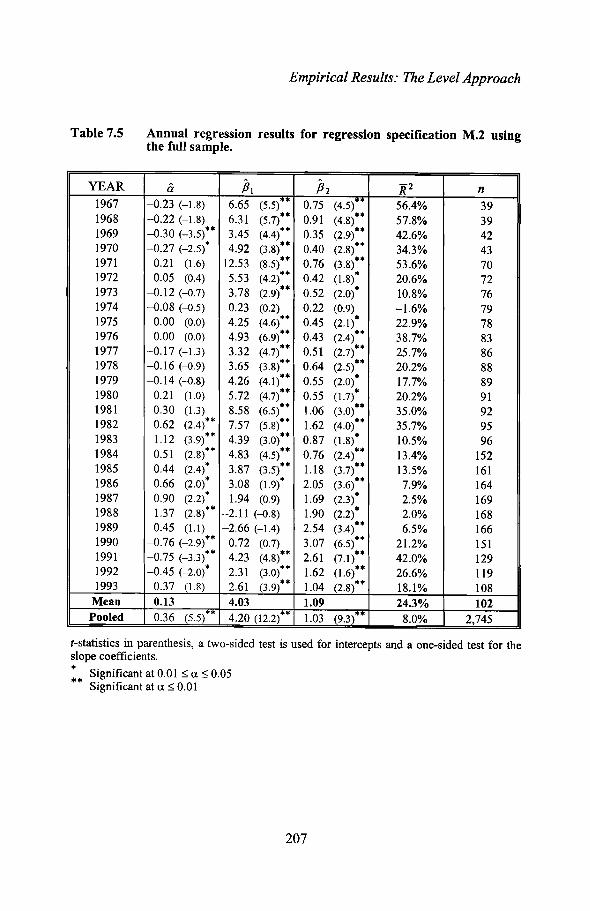
Empirical Results: The Level Approach
Table 7.5 Annual regression results for regression specification M.2 usingthe full sample.
YEAR a PI P2 ]i2 n1967 -0.23 (-1.8) 6.65 (5.5)** 0.75 (4.5)** 56.4% 391968 -0.22 (-1.8) 6.31 (5.7)** 0.91 (4.8)** 57.8% 391969 -0.30 (-3.5)** 3.45 (4.4)** 0.35 (2.9)** 42.6% 421970 -0.27 (-2.5)* 4.92 (3.8)** 0.40 (2.8)** 34.3% 431971 0.21 (1.6) 12.53 (8.5)** 0.76 (3.8)** 53.6% 701972 0.05 (0.4) 5.53 (4.2)** 0.42 (1.8)* 20.6% 721973 -0.12 (-0.7) 3.78 (2.9)** 0.52 (2.0)* 10.8% 761974 -0.08 (-0.5) 0.23 (0.2) 0.22 (0.9) -1.6% 791975 0.00 (0.0) 4.25 (4.6)** 0.45 (2.1)* 22.9% 781976 0.00 (0.0) 4.93 (6.9)** 0.43 (2.4)** 38.7% 831977 -0.17 (-1.3) 3.32 (4.7)** 0.51 (2.7)** 25.7% 861978 -0.16 (-0.9) 3.65 (3.8)** 0.64 (2.5)** 20.2% 881979 -0.14 (-0.8) 4.26 (4.1)** 0.55 (2.0)* 17.7% 891980 0.21 (1.0) 5.72 (4.7)** 0.55 (1.7)* 20.2% 911981 0.30 (1.3) 8.58 (6.5)** 1.06 (3.0)** 35.0% 921982 0.62 (2.4)** 7.57 (5.8)** 1.62 (4.0)** 35.7% 951983 1.12 (3.9)** 4.39 (3.0)** 0.87 (1.8)* 10.5% 961984 0.51 (2.8)** 4.83 (4.5)** 0.76 (2.4)** 13.4% 1521985 0.44 (2.4)* 3.87 (3.5)** 1.18 (3.7)** 13.5% 1611986 0.66 (2.0)* 3.08 (1.9)* 2.05 (3.6)** 7.9% 1641987 0.90 (2.2)* 1.94 (0.9) 1.69 (2.3)* 2.5% 1691988 1.37 (2.8)** -2.11 (-0.8) 1.90 (2.2)* 2.0% 1681989 0.45 (1.1) -2.66 (-1.4) 2.54 (3.4)** 6.5% 1661990 -0.76 (-2.9)** 0.72 (0.7) 3.07 (6.5)** 21.2% 1511991 -0.75 (-3.3)** 4.23 (4.8)** 2.61 (7.1)** 42.0% 1291992 -0.45 (-2.0)* 2.31 (3.0)** 1.62 (1.6)** 26.6% 1191993 0.37 (1.8) 2.61 (3.9)** 1.04 (2.8)** 18.1% 108
Mean 0.13 4.03 1.09 24.3% 102Pooled 0.36 (5.5)** 4.20 (12.2)** 1.03 (9.3)** 8.0% 2,745
I-statistics in parenthesis, a two-sided test is used for intercepts and a one-sided test for theslope coefficients.
* Significant at 0.01 ~ a ~ 0.05** Significant at a ~ 0.01
207

Accounting Information and Stock Prices
Estimated Annual Intercept (a.)
3.0 ..,....--------------------------.2.5 -1------------------------1
--'2.0 • ~
1.5 +---------------.......-=-"":-----..'------'''------1
1.0 ;-----------------4------#~~f-~~..--~------I0.5 -I--------=_------- ~~-----3Il"'==-=~--~-~___=____a
0.0 ----0.5 ;----------------------......---#--1
-1 .0 -+--+--+---<r---+--+---+---+---+--+--+--+--+--+--+--+--+--+--1--+--+--+--+--+---+---+---4('i) LO r--- 0) -r- ('i) LO r---r--- r--- r--- r--- co co co com 0> 0) 0) 0) 0) 0) 0)
-r- -r- -r- -r- -r- -r- -r-
I- · · · M1 M21
Figure 7.4 Estimated annual intercepts (a) for the full sample offirms usingregression specification M.l versus M.2.
7.2.2 Sub-sample regressions controlling for different expectedvalidity of historical ROE and GPF levels
Table 7.6 contains the results of pooled regressions with several differentsub-sample specifications;8 table 7.7 contains the mean of repeated annualregressions for the full sample, the sample divided according to the profitrecognition dimension, and for the homogenized sample.
8 Observe that the regression coefficients (P1 and jJ2) were also significant for all subsamples using White (1980) heteroscedasticity-consistent standard errors. Appendix Sillustrates the regression results for the same sub-samples, but truncating with regard tothe dependent variable-excluding all firm-years when the market-to-book value premium exceeds 4. As a consequence, li 2 is generally sonlewhat higher, A is generallyonly marginally affected, p~ is generally slightly lower and non-significant for a fewof the small more extreme sUb-samples.
208

Table 7.6 Summarized pooled regressions for distinct sub-samples of firms using regression model M.2.
Sample characteristics a fit /32 li 2 n
Full sample 0.36 (5.5)** 4.20 (12.2)** 1.03 (9.3)** 8.0% 2,745
Profit rec. = Continuous 0.20 (3.5)** 5.08 (15.6)** 0.93 (10.5)** 17.9% 1,702Profit rec. = Discrete 0.08 (0.4) 4.09 (5.8)** 2.42 (6.4)** 6.0% 1,043
ROE hist. = Stable 0.40 (3.6)** 5.09 (4.7)** 0.84 (4.9)** 4.3% 998ROE hist. = Intermediate 0.26 (1.8)* 4.87 (5.7)** 1.36 (6.1)** 9.9% 698ROE hist. = Turbulent 0.13 (0.8) 3.11 (7.0)** 1.41 (4.4)** 11.0% 547
Profit rec. = Continuous &ROE hist. = Stable 0.28 (4.2)** 10.39 (13.8)** 0.71 (7.6)** 28.5% 617ROE hist. = Intermediate 0.00 (0.0) 6.58 (7.5)** 1.46 (7.5)** 22.9% 429ROE hist. = Turbulent 0.09 (0.5) 2.47 (4.6)** 1.22 (3.4)** 9.4% 342
E[GPF] = Low 0.24 (1.0) 3.53 (5.2)** 1.40 (5.2)** 8.9% 367E[GPF] =Medium 0.38 (5.2)** 5.20 (9.5)** 1.00 (8.3)** 6.8% 2,246E[GPF] = High 0.00 (0.0) 8.37 (5.0)** 1.23 (2.9)** 21.4% 132
Homogenized sample 0.15 (2.1)** 9.12 (12.8)** 0.99 (l0.1)** 23.9% 941
t-statistics in parenthesis, a two-sided test is used for intercepts and a one-sided test for the slope coefficients.
* Significant at 0.01 ~ a ~ 0.05** Significant at a ~ 0.01

Accounting Information and Stock Prices
Table 7.7 Mean of annual regressions for different sub-samples of firmsusing regression specification M.2.9
Proportion ofSample characteristics a PI P2 li2 n significant
PI years P2 yearsa ~ 0.05 a ~ 0.05
Full sample 0.13 4.03 1.09 24.3% 102 81.5% 96.3%
Profit rec. = Continuous -0.02 4.46 1.04 36.3% 63 81.5% 88.9%Profit rec. = Discrete -0.10 3.98 2.40 16.5% 44 65.2% 73.9%
Homogenized sample -0.07 6.04 1.09 44.1% 38 92.0% 88.0%
Continuous versus discrete profit recognitionIt was earlier observed that for the M.1 specification the explanatory powerof the expected residual return was very weak for the group of firms characterized by a discrete pattern ofprofit recognition (especially for the last 10years of the period being studied). In addition to being suspected of havingless informative reported earnings, these firms can also be expected to haveparticularly large unrealized holding gains. Thus regression specificationM.1 can be expected to be especially under-specified for these firms.
Evaluating M.2 on the observations from discrete profit recognition industries separately, the following observations can be made. The mean GPFcoefficient has increased slightly (from 3.57 to 3.98). The E[RR] variable isnow significant in 65.2% of the annual regressions as compared to the previous frequency of 47.8%.
The inclusion of a PMB estimate in M.2 contributes to a somewhat largermean explanatory power; an Ji2 of 16.5% compared to 11.3% for therepeated annual regressions (and 6.0% compared to 2.9% for the pooledregression). The coefficient related to the PMB (P2) is significant in 73.9%of the annual regressions at the 5 percent level. The mean P2 coefficient is2.40, and it varies between 1.25 and 2.50 for tIle years leading up to the mid
9 A minimum of 10 observations have been required for each annual regression. Thisrequirement leads to the regression coefficients from the early years (1967 - 1972) notbeing included in all sub-sample mean calculations.
210
Empirical Results: The Level Approach
1980s; the period 1985 to 1990 shows slope coefficients amoWlting tobetween 3.0 and 6.0. These latter values indicate quite extreme market-tobook values that are not accompanied by 'sufficiently high' reported ROE.The values can also be interpreted as an indication of that the estimationprocedure of the PMB has on average been too conservative for this groupof firms. Recall from the discussion in Section 3.1.1.3, concerning the levelof partial PMBs related to tangible assets, that long lived tangible assets(held to a large degree in most of the firms in this sub-sample) areparticularly sensitive to the age structure of the portfolio of assets held, andthat any measurement bias would further be magnified the more importantthe partictLlar asset type is for the firm and the lower the equity-to-asset ratioof the firm. A combination of these characteristics that generates a measurement bias for certain firms exceeding lOis not impossible to imagine.The use of industry-constant estimates of the PMBs may thus be particularlynon-representative for the discrete profit recognition firms.
The M.2 specification also increased the explanatory power for the continuous profit recognition group of firms (36.3% versus 26.9% for the mean ofannual regressions, and 19.9% versus 13.4% for the pooled regression).
The PMB coefficients (/32) are significant in 88.9% of the annualregressions at the 5 percent level, and the mean coefficient estimate is in thiscase close to the theoretical value of 1.0 (1.09 in the repeated annualregressions and 0.93 il1 the pooled regression).
Relative stability in ROE historyThe observations that were made when model specification M.1. was usedcan essentially be repeated when M.2 is estimated. Once again, the conclusive observation is that more stable historical returns seem to be associatedwith larger GPFs.l0 Contradictory results in terms of explanatory poweralso appear depending on whether or not the profit recognition characteristics of the sample of firms are controlled for. Given that the continuousprofit recognition firms are used alone, higher ROE stability is also relatedto higher explanatory power.
10 PI = 10.4, 6.6 and 2.5 for the stable, intermediate, and the turbulent ROE historygroups respectively, when only firms from continuous profit recognition industries areincluded in the regressions.
211

Accounting Information and Stock Prices
Expected GPFThe observations that were made when model specification M.1 was used,can be repeated when M.2 is estimated. The level of the estimated GPF coefficients (PI = 3.5, 5.2 and 8.4 for the low, medium, and the high GPFgroups respectively) supports the validity of the classification. One can further note that the added PMB variable is significant in all three sub-samples(with a value of 1.40, 1.00 and 1.23, for the three sub-samples respectively)and improves the total explanatory power somewhat.
A homogenized sample-combining ROE validity criteria andcontrolling for extreme GPFsThe results for the homogenized sub-sample are found in the last row of thesummary tables above, in a complete annual presentation in table 7.8, andthe annual regression results are contrasted with the full sample regressionresults in figures 7.5, 7.6 and 7.7.11
11 The homogenized sub-sample was selected according to the following criteria: i) Thefirm belongs to an industry classified as having continuous profit recognition, ii) thefirm has a non-turbulent ROE track-record (the standard deviation of the past five yearshas not exceeded 10%), and iii) the expected growth persistence factor is classified asmedium.
212

Table 7.8
Empirical Results: The Level Approach
Annual regression results using regression specification M.2 andobservations for the homogenized sub-sample.
YEAR Ii Pi P2 ]i2 n196719681969 -0.27 (-2.3)* 3.22 (2.4)* 0.34 (2.1)* 26.2% 291970 -0.27 (-2.1)* 5.03 (2.9)** 0.40 (2.3)* 28.4% 311971 -0.02 (-0.2) 10.17 (6.2)** 0.74 (5.8)** 67.8% 341972 -0.16 (-1.4) 4.15 (2.9)** 0.42 (2.9)** 32.4% 341973 -0.14 (-0.9) 8.40 (3.3)** 0.39 (1.7)* 19.6% 451974 -0.17 (-1.1) 3.69 (1.9)* 0.19 (0.8) 5.0% 381975 -0.06 (-0.5) 4.93 (3.2)** 0.32 (1.9)* 22.9% 361976 -0.01 (-0.1) 5.72 (3.6)** 0.28 (1.8)* 35.5% 311977 -0.25 (-2.3)* 4.81 (4.0)** 0.47 (3.8)** 49.0% 301978 -0.37 (-2.5)* 5.75 (3.3)** 0.65 (4.6)** 59.4% 311979 -0.46 (-4.8)** 4.20 (4.2)** 0.55 (5.0)** 55.8% 381980 -0.18 (-1.8)* 6.70 (7.3)** 0.63 (5.0)** 65.0% 401981 -0.38 (-3.0)** 5.42 (4.8)** 1.07 (7.2)** 65.4% 391982 -0.47 (-1.3) 5.45 (l.8)* 2.32 (7.0)** 68.6% 391983 0.13 (0.6) 7.18 (3.2)** 1.69 (6.2)** 57.1% 401984 -0.23 (-0.2) 1.22 (0.7) 0.93 (5.2)** 44.7% 381985 0.03 (0.2) 5.52 (3.6)** 1.18 (6.5)** 66.4% 371986 0.45 (l.8) 7.12 (2.6)** 1.56 (4.2)** 31.2% 551987 0.68 (2.9) 7.14 (2.6)** 1.12 (3.1)** 23.5% 611988 0.94 (1.2 3.55 (0.5) 1.79 (1.4) 0.7% 571989 0.44 (1.4) 10.24 (2.9)** 1.94 (4.4)** 37.6% 511990 -0.56 (-2.0) 9.67 (4.5)** 2.86 (6.9)** 67.5% 431991 -0.76 (-2.4)* 7.51 (3.3)** 2.86 (6.7)** 78.8% 241992 -0.28 (-0.6) 9.22 (2.7)** 2.10 (3.7)** 75.2% 201993 0.56 (1.2) 5.10 (2.3)** 0.44 (0.6) 18.1% 20
Mean -0.07 6.04 1.09 44.1% 38Pooled 0.15 (2.1)** 9.12 (12.8)** 0.99 (10.1)** 23.9% 941
t-statistics in parenthesis, a two-sided test is used for intercepts and a one-sided test for theslope coefficients.
* Significant at 0.01 s a S 0.05** Significant at a S 0.01
213
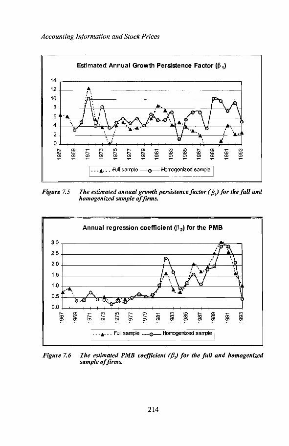
Accounting Information and Stock Prices
Estimated Annual Growth Persistence Factor (~1)
...~ ~ 10 I'-I'- I'- I'- I'-0') 0') 0') 0')~ ~ ~
14 __--------------------------.
12 +----------7"""::-------------------------1
10 -t-------rl'~---------------____\~__-____I
8-t------I--\o----1""'\--------.....=--=~-----_f_-_+=;:-I-_\__I
6 -
4 +--..-----;,~-----c~.--)".~.r___~ ........---___=_t______,FA_-_____\:J___-_4~___I
2+-----------.-----t----------\-I----A-----.----~
o-+--+-+-+--+--!---+ ~___+____+__+___+___+_____+_____+__+__+__+__+_..,.......+_+__+--~~
E Full sal1llle -e-- I-t>rrogenized sal1llle '
Figure 7.5 The estimated annual growth persistence factor (PI) for the full andhomogenized sample offirms.
Annual regression coefficient «(32) for the PMB
3.0
2.5
2.0
1.5
1.0
0.5
0.0...... 0') ~ ~co co I'- I'-m 0') 0') 0')
~ ~
I...&••• Full sal1llle -e--I-t>rrogenized sal1llle I
Figure 7.6 The estimated PMB coefficient (P) for the full and homogenizedsample offirms.
214

Empirical Results: The Level Approach
R2 for different sub-samples
90% -r-----------------------__80% -I------------------------.~___1
70% -I---- -------------:~-____=~--- -_t__I
60% +-::-::..----------t-1r---------f!'8l~~-~ _t_'\__--_I----_t__I
50% -I--------'-r---f~_+__---~~----_r__I___+__----I---_+_I
40% -I----!!!!!-...--..l=----'4------.J---------+-------:lI~--flllailr__+_I
30% -I-----&----'i"\---~---'r---__.''----'-------.--------f------~_+I
20% +-----~__r;~-r--______=,a _:A_---T---~-E__......._-~
10% +-------A+~._------ .....=_=_--=--,......_--+_I_:-t----_I
0% +--+__+--+--+---+--of---l,..:.....+--+---l--+---+--+-+--I---+---+---+---+-~l»--+__+--+-__+_ .....
to PJ r:::(J) (J) (J)"l"'"" "l"'""
I·· .•... Full sarrple ----+--I-brrogenized sarrple I
Figure 7. 7 The adjusted explanatory power (li 2 ) for each annual estimation ofregression specification M.2 for the full and homogenized sample offirms.
The GPF coefficient (/31) is positive and significant at the 5 percent level in23 of the 25 annual regressions. In 20 of the 25 regressions the level of significance further exceeds the 1 percent level. The PI coefficient varies between 3.22 and 10.24 for the years when it is significant (the insignificantyear, PI is still positive, but only amounts to 1.22). In comparison to the previously presented regression results using M.l and the same sample specification, it is noteworthy that the mean GPF coefficient has been reducedfrom 8.54 to 6.04 and is somewhat more stable over time. Most coefficientsvary between the economically reasonable values of4 and 8.
The regression coefficient for the estimated PMB parameter is on average1.09, and exceeds zero significantly in 22 of the 25 annual regressions at the5 percent level. The /32 coefficient varies between 0.32 and 2.86 for theyears when it is significant (in the insignificant years, /32 also shows positive values). The value of the coefficient over time shows a very similarpattern for the homogenized sample compared with the full sample (seefigure 7.6), a rather stable coefficient around 0.5 until the early 1980s whenthe coefficient value increases and becomes rather variable over the years.
215

Accounting Information and Stock Prices
The average adjusted explanatory power of the regression is 44.1 %, withtwo years (1974 and 1988) standing out as being particularly poor. It isfurther noteworthy that the explanatory power is also lower than 'normal'in the years surrounding these two particularly poor years (see figure 7. 7).A similar but less distinct pattern is present for the full sample.
Several alternative factors offer a conceivable explanation for this pattern:1. the two periods coincide with two particularly large fluctuations in the
Swedish business cycle (see Section 5.2.2);2. the first period coincides with the start of a 'new era' of a higher infla
tion rate (see Section 5.2.1);3. both the periods coincide with periods of particularly uneven accounting
practices (transition periods), the first concerning open disclosure ofvalue and depreciation according to plan and group consolidationmethod, the second related to the goodwill issue and accounting forassociated companies (see Section 5.3).
Further investigation of these issues will be undertaken in the forthcomingsections.
216

Empirical Results: The Level Approach
7.3 Regression results and changes in theeconomic climate
7.3.1 Business cycle fluctuationsFigure 7.8 illustrates the median market-to-book value premium each yearalong with the indicator of the business cycle identified in Section 5.2.2.
The Market-to-Book value premium in differentbusiness cycle phases
-r-----------------------,.. 70
--1-----#--...-------------------...-----4 60 Co50 ~
+--.----.----I-~------___{::::'J-=-----+_#=_-----.:l~--___1 N
40 ~-+-#---~-I--~--~~___.:___.:....ct')<ll''------______..k__-_\9i :::J
30 CD~
20 g10 ::
r:t:
2.0
1.5
1.0~.
0.5co-....:E
0.0
-0.5
-1.0t'- (j) r:: ('f)<0 <0 t'-0) 0') 0) (j)"r" "r" "r"
1- - - e- - - Market-te-Book - 1---Resource utilization 1
Figure 7.8 The median market-to-book value premium for the full samplecombined with an index of the Swedish industrial resource utilization. 12
After a period of rather stable market-to-book value premiums around orslightly below zero that ended in 1981, the premiums show increasing variability around much higher values. During the latter more variable period, apositive co-variability between the business cycle phase and the market-tobook value premiun1 is quite obvious.
In order to investigate whether fluctuations in the business cycle are an important source of instability of explanatory power and value of the regression coefficients when attempting to explain the market-to-book value pre-
12 The weighted sum of reported incidences of full capacity utilization and labor shortagesin the Swedish industrial sector. Source: "Business Tendencies Surveys", NationalInstitute of Economic Research.
217

Accounting Information and Stock Prices
mium with M.2, the annual regression results from the previous section areplotted together with the business cycle indicator. Figures 7.9,7.10,7.11and 7.12 contrast the adjusted explanatory power, and the three regressioncoefficients for each annual regression using the full sample with the phasesof the business cycle.
R2 in different business cycle phases
60%> 70
~'.50°1'0 60 S40% 50 ~
N
R2 30°1'040 ;S
;:,30 CI)
20% CJ20 :;
010% 10 ::
D:0% \ . 0
........ <J) r:: (\') LO ........ <J) ex; (\') LO ........ m ~ C")co co ........ ........ ........ ........ co co co co m m<J) <J) (j) <J) (j) <J) m m m m m m m m~ ~ T'"" ~ ~ ~ ~ ~ ~ ~ ~ ~
.•.~••. Explanatory power ---Resource utilization
Figure 7.9 The adjusted explanatory power (]i2) for each annual estimation ofregression specification M.2 for the full sample offirms combinedwith an index ofSwedish industrial resource utilization.
218
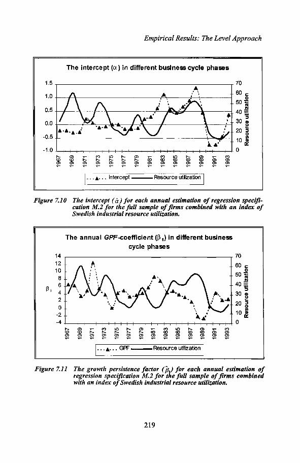
Empirical Results: The Level Approach
The intercept (a) in different business cycle phases
~ (t') lC) ,.... 0') 0; (W)co co co co co 0')0> 0') 0') 0') 0> 0> 0')~ T"'" T"'" T"'" T"'" T"'" T"'"
Resource utnization II. ..•. .. Intercept ---
0.5 +---I---~-_#_~..___-----~-~~;#_-~---__i
1.0 -+----4--.----------~_+__-- .a.----___I
1.5 _.___---------------------__ 70
60 co
50 ;:;:J
40 S::J
0.0 -I-----...=---=---~______..____ '6__-I__~-___..~----~--~ 30 820 5o10 :
D:-I-~r___+--+_+__+__+_+_+__+__+__l__+__+_+_~r___+_+_+__+__+_+_+__+__+__+O
-0.5
-1.0,.... 0') r::: (t') LO ,.... 0')co co I'- I'- I'- I'-0') 0') 0') 0') 0') 0') 0')T"'" ~ T"'"
Figure 7.10 The intercept (a) for each annual estimation of regression specification M.l for the full sample offirms combined with an index ofSwedish industrial resource utilization.
The annual GPF-coefficient (~1) in different businesscycle phases
0> «; (W) LO ,.... 0') 0; (W)I'- co co co co 0')0> 0') 0) 0) 0) 0) 0) 0)T"'" T"'" T"'" T"'" T"'" T"'" T"'" T"'"
Resource utilization 1
__---------------------__ 70
60 co
50 ;:;:J
40 =="S
30 CD~
20 ~
10 i+--+--+-+--+-.....j--+-+--+--+---+--+--+-l-+--+---+--+--+--+--+---+-.....j--+--l~--+---I--O
I GPF---
141210
8
~l6420
-2-4
I'- 0') r::: (W) LO I'-co co I'- I'- I'-0') 0') 0> 0') 0') 0>T"'" ~ ~ ~ T"'" T"'"
Figure 7.11 The growth persistence factor (p) for each annual estimation ofregression specification M.l for the full sample offirms combinedwith an index ofSwedish industrial resource utilization.
219
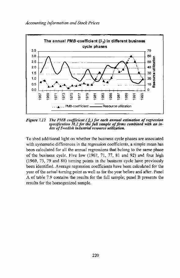
Accounting Information and Stock Prices
The annual PMB-coefficient (~2) in different businesscycle phases
3.5 ,.....----------------- -,- 70
3.0 60 co
2.5 50 ~N
2.0 40 ~:J
1.5 30 ~
1.0 20 S05 10 =. ~
0.0 0
1_ - . A- _. PMB-coefficient ---Resource utilization I
Figure 7.12 The PMB coefficient (82
) for each annual estimation of regressionspecification M.2 for the full sample offirms combined with an index ofSwedish industrial resource utilization.
To shed additional light on whether the business cycle phases are associatedwith systematic differences in the regression coefficients, a simple mean hasbeen calculated for all the annual regressions that belong to the same phaseof the business cycle. Five low (1967, 71, 77, 81 and 92) and four high(1969, 73, 79 and 88) turning points in the business cycle have previouslybeen identified. Average regression coefficients have been calculated for theyear of the actual turning point as well as for the year before and after. PanelA of table 7.9 contains the results for the full sample; panel B presents theresults for the homogenized sample.
220

Empirical Results: The Level Approach
Table 7.9 Mean of annual regressions for different years clustered on business cycle phase using regression specification M.2.
P IAThfllane : e u sampe
Proportion of
a Pi /32 ]i2 n significant/31 years P2 yearsa ~ 0.05 a ~ 0.05
All business cycle phases 0.13 4.03 1.09 24.3% 102 81.5% 96.3%
Year before top 0.14 4.36 0.92 25.3% 92 75.0% 100.0%Top (1969, 73, 79, 88) 0.21 2.35 0.83 18.3% 94 75.00k 100.0%Year after top 0.08 2.05 0.92 14.9% 95 50.0% 75.0%
Year before bottom -0.20 4.95 1.00 33.8% 87 100.0% 100.0%Bottom (1967,71,77,81,92) -0.07 6.68 0.94 39.5% 81 100.00k 100.0%Year after bottom 0.13 5.14 0.92 30.5% 80 100.0% 100.0%
P IB Th h · dane : e om02enlze samJ e
Proportion of
a Pi P2]i2 n significant
PI years P2 yearsa ~ 0.05 a ~ 0.05
All business cycle phases -0.07 6.04 1.09 44.1% 38 92.0% 88.0%
Year before top 0.05 5.68 0.73 38.4% 42 100.0% 100.0%Top (1969, 73, 79, 88) 0.02 4.84 0.77 25.60/0 42 75.0% 75.0%Year after top -0.04 6.41 0.79 34.0% 40 100.0% 75.0%
Year before bottom -0.30 6.24 1.04 51.9% 32 100.0% 100.0%Bottom (1971, 77, 81, 92) -0.23 7.40 1.10 64.4% 31 100.00/0 100.00kYear after bottom -0.11 5.11 0.96 44.6% 31 100.0% 75.0%
Figure 7.9 gives a visually very convincing indication of a negative association between the explanatory power of M.2 and the phase of the businesscycle. The adjusted R2 is lower in and around the boom periods of the economy, and higher in and around a recession. This association is corroboratedby the mean ]i2 in table 7.9. The mean ]i2 is 18.3% vs. 39.5% and 25.6%vs. 64.4% at the top versus the bottom of the business cycles for the full andthe homogenized sample respectively. A similar pattern, but not as pronounced, is present in the surrounding periods.
221

Accounting Information and Stock Prices
At least for the latter half of the period studied, the value of the interceptseems to be positively associated with the phase of the business cycle. Notethe co-movement in figure 7.10 from 1980 onwards. This observation isstrengthened by the generally positive mean intercepts for the boom periodsversus negative mean intercepts in recessions, as illustrated in table 7.9.
A negative association is evident between the value of the GPF coefficient(Pt) and the phase in the business cycle. This is visually obvious from figure7.11 and corroborated by the mean coefficients in the table. The mean PI is2.35 vs. 6.68 and 4.84 vs. 7.40 at tIle top versus the bottom of the businesscycles for the full and homogenized sample respectively.
Finally, the coefficient related to the PMB variable (/32)' also seems to benegatively associated with the business cycle phase. This pattern is mostobvious in the latter half of the period when the coefficient is more variable.
These results clearly support the hypothesis that some ofthe intertemporalinstability in the cross-sectional regression coefficients are related to thefluctuations in the business cycle. An unresolved question is why thispattern is present?
• First of all, the positively varying intercept indicates that the valuationspecification lacks some explanatory variable.
• In a discussion of the estimation of 'T', the expected period over whichabnormal performance can be defended, Stewart (1991, p. 298) arguesthat the length of time (beyond specific business characteristics) maydepend on the general economic and political outlook. He exemplifiesthis with the optimistic times of the 1960s and the pessimistic times ofthe 1970s. One could thus (contradictory to the regression results) arguefor higher expected GPF coefficients in booming periods due to assumingly more optimistic times.
• One may suspect that the unstable results are to some extent driven byth~ primitive estimation procedure of expected ROE. If investors canforesee the changes in the business cycle, and adjust their expectationsaccorditlgly, a prediction of next period's ROE based on the most recentperiod's performance may be a particularly unreliable approach aroundthe fluctuations in the business cycle. In Chapter 4, the option of usingearnings forecasts from business magazines was ruled out as an earnings
222

Empirical Results: The Level Approach
prediction input in this study. The lack of such data for the entire periodwas the main obstacle. However, since February 1985 Affarsvarlden (aSwedish business weekly) has on a weekly basis published forecasts ofthe coming years' earnings per share for firms listed on the StockholmStock Exchange. To shed some light on the importance of utilizing anexpectation procedure based on the most recent period's reported ROErather than this business press alternative, the regression specificationM.2 has been re-run for a small group of companies usingAffarsvarlden's published earnings forecasts. Details regarding thisendeavor are found in appendix T. The results indicate thatAffarsvarlden's earnings forecasts better nlap expectations on the stockmarket than the simple estimation procedure utilized in the main part ofthis study. It is observed that the mechanical historic performancemethod seems to be somewhat 'noisier', but that the two return on equityestimation procedures seem to capture essentially the same phenomena.It is further demonstrated that the negative association between the explanatory power of M.2, and the phase of the business cycle, remainseven when Affarsvarlden's earnings forecasts are used.
• Finally, consider the following statement from a player on the stock market during the booming period of the 1980s: "There is no time for fundamental analysis in a booming market, investors just have to act." If sucha statement bears any resemblance to actual behavior, it would be consistent with a case when many companies tend to be valued high irrespective of performance in good times, whereas quality performanceyields a stronger premium in bad times. Such a scenario is consistentboth with the observation of higher GPF coefficients and higher ]i2 inrecessions and vice versa in booming periods.
223

Accounting Information and Stock Prices
7.3.2 Changes in the rate of inflationIn Section 5.2.1 four inflation rate phases occurring during the period 1967to 1993 were identified.
ABCD
Time period1967 - 19721973 - 19801981 - 19841985 - 1993
Inflation rate characteristicsLow
Rising-low to highHigh
Falling-high to nledium
It was argued that the increasing inflation rate of the early 1970s could beexpected to decrease the informative value of traditional accounting basedprofitability ratios, especially for firms whose asset base is dominated bynon-monetary assets with long economic lives. Also, the period with a sharpfall in the inflation rate (1985-1987) was hypothesized to be especiallyproblematic. To test whether these phases are associated with anysystematic differences in the regression coefficients, the mean of annualregressions have been clustered for the four phases. The mean of the firsttwo years of each 'problematic' period is also going to be reportedseparately. In table 7.10, the M.2 regression results for the full sample arepresented, followed in table 7.11 by similar M.1 regression results for twoextreme sub-samples. These two sub-samples were generated in Section5.2.1, in an attempt to maximize the difference in tendency to hold nonmonetary assets with long economic lives. It can be noted that the estin1atedPMBs are almost constant within the two subgroups. It is thus not meaningful to use regression specification M.2 for the separate sub-samples.However, the higher expected PMBs for the group of firms holding largeamounts of non-monetary long-life assets is expected to be captured by alarger intercept (a) in specification M.1. -
224

Empirical Results: The Level Approach
Table 7.10 Mean of repeated annual M.2 regressions for different time-clusters based on inflation rate characteristics.
Proportion of
Full Sample a Pi P2]i2 n significant
Pi years fJ2 years(1::;0.05 (1::;0.05
All years 0.13 4.03 1.09 24.3% 102 81.5% 96.3%
A: 1967-72 -0.13 6.57 0.60 44.2% 51 100.0% 100.0%B: 1973-80 -0.06 3.77 0.48 19.3% 84 87.5% 87.5%C: 1981-84 0.63 6.34 1.08 23.7% 109 100.0% 100.0%D: 1985-93 0.25 1.55 1.97 15.6% 148 55.6% 100.0%
Early B: 1973-74 -0.10 2.01 0.37 4.6% 78 50.0% 50.0%Early D: 1985-86 0.55 3.47 1.62 10.7% 163 100.0% 100.0%
Some notable observations emerge from the regression results for the fullsample. The mean explanatory power (Ji2) for the low inflation rate period,prior to 1973, is 44.2%, which is almost twice as high as in any of the following periods. The mean ]i2 is particularly low during the rising and falling inflation rate periods (period B and D). During these inflationary problematic periods, the frequency of significant regression coefficients is thelowest.
One may also note that /32-the slope coefficient of the estimated PMBsfollows a pattern similar to the general inflation rate development, but witha lag. The estimated PMBs were specified to reflect issues relating to theholding of assets that are not captured in traditional accounting. With anideal n1easurement procedure of the PMBs, /12 should thus be expected toequal one. However, in this study the PMBs were (for simplicity) assessedto be constant over time, utilizing the average inflation rate as a proxy forvalue change. The below average inflation rates during the early years of thestudy followed later by higher inflation rates, will thus result in overstatedPMBs in the early periods and vice versa, and could thus be one plausibleexplanation for the development of the /3 2 coefficient. Annual re-estimationof the PMB is an improvement that could possibly reduce this instability.
225

Accounting Information and Stock Prices
Table 7.11 Mean of repeated annual M.l regressions for different time-clusters based on inflation rate characteristics.13
ttfdtane : lrms 0 ln~ an ex enSlve e 'ree 0 non-mone ary on2- I e asse s
Extensive long-life Proportion of
asset frrms a /31 R2 n significant iJ1 yearsa. ~ 0.05
All years 1.40 6.70 21.2% 30 56.5%
A: 1971-72 0.97 16.97 66.0% 18 100.0%B: 1973-80 0.76 6.93 27.9% 21 75.0%c: 1981-84 1.56 8.30 22.2% 29 50.0%D: 1985-93 1.98 3.50 4.9% 41 33.3%
Early B: 1973-74 0.56 4.41 12.4% 17 0.0%Early D: 1985-86 2.42 9.35 6.3% 39 50.0%
ttflIdane : lrms 0 ln~ a sma e2ree 0 non-mone ary on2- I e asse s
Limited long-life Proportion of
asset frrms a PI R2 n significant lJ1 yearsa. ~ 0.05
All years 0.40 4.93 31.5% 26 82.6%
A: 1971-72 0.30 14.64 53.5% 20 100.0%B: 1973-80 -0.04 3.48 31.1% 20 87.5%C: 1981-84 0.61 4.26 34.8% 24 75.0%D: 1985-93 0.72 4.37 25.4% 34 77.8%
Early B: 1973-74 0.01 2.21 7.5% 23 50.0%Early D: 1985-86 0.83 6.38 39.6% 45 100.0%
The previous observation of weakened explanatory power after the new eraof higher and Inore variable inflation rates can be made again with regard toboth sub-samples. This tendency, however, is stronger for the 'Iong-lifeasset sample'. The most striking difference between the two subgroupsoccurs during the period 1985-93 with falling inflation rates. The 'Iong-lifeasset firms " show very weak regression results during this period. The overall mean explanatory power is very poor (4.9% during 1985 to 1993), andthe expected residual return variable is only significant in three of the nine
13 The years between 1967 and 1970 have been excluded due to a limited number ofobservations.
226

Empirical Results: The Level Approach
years on the five percent level. For the llimited long-life assets sample' theexpected residual return variable is significant in seven of the nine years onthe five percent level, and the mean explanatory power remains just above25% for the same time period.
As a general observation, one can note that a is consistently larger for theIZong-life asset sample' (1.40 as compared to 0.40 for all years), with aneven more pronounced difference for the years with falling inflation. This isconsistent with the fact that the clong-life asset sample' firms tend to holdassets for which value gains are not fully captured within the traditionalhistorical cost accounting procedure (until realization). The median PMB forthe two sub-samples are 0.67 and 0.31 respectively. For this reason, thevalue of a, especially for the IZong-life asset sample', indicates that thePMB estimation on average has been 'too conservative' or possibly thatsome fundamental variable that explains the level of the market-to-bookvalue premium is missing in the specified valuation model.
227

Accounting Information and Stock Prices
7.4 Regression results and large accounting changes
7.4.1 Open disclosure of depreciation according to planIn Section 5.3.1 a gradual transition in accounting practice regarding depreciation and valuation of depreciable assets was observed, from a tax-basedpractice to a practice attenlpting to describe value and depreciation in accordance with the estimated economic lives of the assets. The transitionessentially took place between 1967 and 1980, with the strongest changebetween 1975 and 1976. The three figures below illustrate the annualaverages of the dependent and independent variables for the sample groupedaccording to tIle chosen accounting practice.14
Market-to-book value premium
1.0 __----------------------,0.8 +-----------------------t
0.6 +-----------------------1
0.4 +----------------------t
0.2 £:::'1:::----------------,,----------,L
0.0 . -A... ..-~ -
-0.2 +-------~::__--~~___==------____I-0.4 +----------------==--"""-o;;iI~ ___v
-0.6 +----t-----+----+---.....,-.---+-----+---~
1971 1972 1973 1974 1975 1976 1977 1978
I--<i>-- Open disclosure ••••••• Non-open disclosure!
Figure 7.13 The annual averages of the market-to-book value premium for twosubgroups offirms using different depreciation practice.
14 Recall from Section 5.3.1, that the industries with firms that are expected to hold relatively small an10unts of depreciable assets have been excluded. Note also that thenUITlber of observations (firms) behind each average varies considerably over time(from 5 to 44). With this shortage of annual data, annual regressions controlling foraccounting procedure are difficult to carry out. Therefore pooled regressions have to beused.
228

1972 1973 1974 1975 1976 1977 1978
Empirical Results: The Level Approach
E[RR]
15°t'o ..,...--------------------.......
100/0 -1-----------------------1
5°1o -t----------------------t
00/0 -t----~--=-~_=__~~___=:_a__-~=________:=_=A_--___i
-10°10 +-----------------=~_~=J¥'
-15°10 +-----1r-----+----1---+----f------+----I
1971 1972 1973 1974 1975 1976 1977 1978
I----+-- Open disclosure ••••••• Non-open disclosure I
Figure 7.14 The annual averages of the expected residual for two subgroups offirms offirms using different depreciation practice.
PMB
1.00 C:'l------------------------,
0.75 -I-----~:::::::::::~~==!!!iG___==_-------I
0.50 ........, ........-----j..............------..~----- _.__.___, _A_____'lL.:!:----__.. . A·· .. - .
0.25 +---------------------------i
0.00 +----t--------I----+---+----fo----+---......
1971
I----+-- Open disclosure ••.•••• Non-open disclosure I
Figure 7.15 The annual averages of the estimated permanent measurement bias(PMB) for two subgroups of firms using different depreciationpractice.
A number of observations can be made from these figures. Figure 7.15 suggests that the early open-disclosure firms are different in this dimension.
229

Accounting Information and Stock Prices
The early adopters have a higher measurement bias. 15 This group containspharmaceuticals, R&D-intensive engineering firms, and paper & pulp firms.When most firms have changed to open disclosure towards the end of theperiod, this difference has vanished. The average E[RR]16 is essentiallyequivalent for both groups during the early years in the graph. Towards theend of the period (that includes the beginning of a recession), the group ofnon-open disclosure firms shows a mean residual return that remains ataround zero, while the group of open disclosure firms shows a return thatdrops considerably.17 One explanation for this result can be that the nonopen disclosure firms have accumulated hidden untaxed reserves, in earlierperiods, that they choose to dissolve in a recession to show positive earnings. The subgroup of firms disclosing asset values according to economicplan consistently show a lower average market-to-book value premiumcompared to the other subgroup (1971 being an exception).l8 Given similarPMB and E[RR] this is not unexpected as these firms, ceteris paribus, showa relatively higher book value of equity.19
Pooled regression results for the two subgroups are showed in table 7.12.The pooled regressions are run for the period 1967 to 1980, 1971 to 1978,and finally also for two main transition years, 1975 to 1976 (panel A, B, andC). Since the observations in these three sub-periods do not constituteindependent samples, the regression results are also provided for twoseparate periods: 1970 to 1974 and 1975 to 1978 (panel D and E).
15
16
17
18
19
The mean difference in PMBs is significant, at the 5 percent level, as a total over theperiod 1971 to 1978, and the differences are also significant for each individual yearbetween 1971 and 1975, but not thereafter.Given the estimation procedure of E[RR], utilizing the most recent published ROE,these figures can be interpreted as cost of equity normalized ROE.The mean difference in E[RR] is significant, at the 5 percent level, as a total over theperiod 1971 to 1978, and the differences are also significant for each individual yearbetween 1975 and 1978, but not before.The n1ean difference in market-to-book value premium is significant, at the 5 percentlevel, as a total over the period 1971 to 1978, and the differences are also significant foreach individual year between 1975 and 1978, but not before.(1-1') times the disclosed untaxed reserve is included in the equity calculation given thatthe untaxed reserve is openly disclosed.
230

Empirical Results: The Level Approach
Table 7.12 Pooled regression results using regression specification M.2and all firm years from nine industries with firms where themost depreciable assets are held.
Panel A: 1967-80
1967-80 a PI /32 ]i2 nAll firms -0.26 (-7.7)** 2.92 (12.9)·· 0.43 (8.9)** 26.4% 682
Non-disclosure -0.08 (-1.0) 4.68 (9.4)** 0.30 (1.8)* 24.9% 263Open disclosure -0.50(-11.6)** 2.09 (7.5)** 0.55 (11.7)** 47.3% 252
Panel B: 1971-78
1971-78 a PI P2 ]i2 nAll finns -0.21 (-4.8)** 2.62 (9.1)** 0.35 (5.3)·· 20.3% 427
Non-disclosure 0.00 (0.1) 4.10 (5.7)** 0.15 (0.7) 16.5% 153Open disclosure -0.53 (-9.5)** 1.90 (5.4)** 0.54 (9.5)** 48.5% 149
Panel C: 1975-76
1975-76 a PI /32 ]i2 nAll firms -0.12 (-1.8) 3.69 (7.7)·· 0.32 (3.2)** 38.3% 107
Non-disclosure 0.00 (0.0) 3.52 (3.0)** 0.28 (0.8) 18.2% 33Open disclosure -0.35 (-3.7)** 3.41 (5.0)** 0.45 (5.2)** 64.3% 37
Panel D: 1970-74
1970-74 a PI /32 ]i2 nAll firms -0.19 (-3.2)** 2.45 (4.9)** 0.31 (3.3)*· 11.2% 251
Non-disclosure -0.04 (-0.3) 4.87 (5.7)** 0.17 (0.7) 19.0% 131Open disclosure -0.44 (-4.3)** 1.65 (1.8)* 0.44 (4.1)** 33.6% 33
Panel E: 1975-78
1975-78 a PI P2 ]i2 n
All firms -0.26 (-4.7)** 2.74 (8.3)** 0.42 (5.4)** 31.4% 215
Non-disclosure 0.01 (0.1) 3.21 (3.6)** 0.25 (0.9) 20.2% 46Open disclosure -0.56 (-8.2)** 1.87 (4.5)** 0.59 (8.3)** 48.1% 118
t-statistics in parenthesis, a two-sided test is used for intercepts and a one-sided test for theslope coefficients.
* Significant at 0.01 ~ a ~ 0.05** Significant at a ~ 0.01
The ]i2 is approximately twice as high for the lopen disclosure firms' compared to the Inon-disclosurefirms' (47.3% vs. 24.9%) for the whole transi-
231

Accounting Information and Stock Prices
tion period 1967 to 1980; the difference increases to more than three times(64.3% vs. 16.5%) for the main transition period 1975 to 1976. Differencesof the same magnitude can be observed for the two separate---early andlate-periods presented in panel D and E. These results indicate that themarket-to-book value premium is better explained by the residual return andthe PMB variable for the firms with open disclosure of value and depreciation of tangible assets. The more informative, open accounting procedure,thus appears to be associated with a better mapping to the stock price.
In order to test if these results are driven by some systematic difference inthe sub-samples, the same regressions have also been run using the homogenized sub-sample.20 Complete results are reported in appendix U. Theseresults indicate an informative advantage that is at least as strong for opendisclosure firms. The adjusted R2 for the period 1967 to 1980 is, for example, 62.5%, 23.1%, and 36.4%, for the open disclosure, the non-disclosure,and all the firms respectively. These values indicate that the uneven (anduninformative) accounting practice has a strong detrimental effect on theexplanatory power of the valuation specification.
Besides the lower explanatory power for the non-disclosure firms, one canalso note that the /32 coefficient is lower and most often non-significant.The main reason for this appears to be a lower variation of the PMBs withinthis group of firms. It is important to note, however, that the differences insignificance related to the PMB alone do not drive the overall results. A rerun for the period 1967 to 1980 using regression specification M.l on thehomogenized sample, after excluding all observations when the PMB exceeds 0.50, resulted in an explanatory power of 47.2% vs. 25.7% for theopen disclosure vs. non-disclosure sub-samples.21
20 i) The firm belongs to an industry classified as having continuous profit recognition, ii)the firm has a non-turbulent ROE track-record (the standard deviation of the past fiveyears has not exceeded 10%), and iii) the expected growth persistence factor is classified as medium.
21 Similar differences also remained for the other periods.
232

Empirical Results: The Level Approach
7.4.2 Regression results and acquisition actfvityIn Section 5.3.2 the period 1986-1990 was identified as being unique interms of acquisition activity among the firms listed on the Stockholm StockExchange. Whether this acquisition activity has had an impact on the relationship between market-to-book value premiums and expected return is thefocus of this section. The sample has been divided in two subgroups: i) an'acquisition group'-where at least one recent large acquisition has takenplace, and ii) a 'no acquisition group '-where no recent acquisition hastaken place. 22
Reduced stability of ROE is one potential effect of an acquisition. The sample control criteria related to stability of historical ROE should thus not beapplied. However, in order to improve the control of the sample, only thefirms from industries classified as having a continuous profit recognitionhave been used.23
In order to check for systematic differences between the two groups in termsof the dependent and independent variables, the mean market-to-book valuepremium, the mean E[RR], and the mean PMB have been calculated.24 Ascan be seen from figure 7.16, the mean market-to-book value premiunls ofthe two subgroups have been practically identical (this is also true for themean PMB, graph not provided).25 Neither do the mean E[RR]s-illustratedin figure 7.17-give any indications of systematic differences between thetwo subgroups.
22
23
24
25
A firm has been classified as having made a recent acquisition during a particular yearif such an acquisition has taken place during the current year or during any of the twopreceding years. See details regarding the identification procedure of acquisitions inSection 5.3.2.This choice gives an improved explanatory power for all the regressions, but appearsnot to make any qualitative difference in terms of relative explanatory power.The period illustrated has been extended to 1992 in order to include the two years afterthe most acquisition-intensive period (1986-1990).The slightly higher mean market-to-book value premium for the acquisition group isnot significant.
233
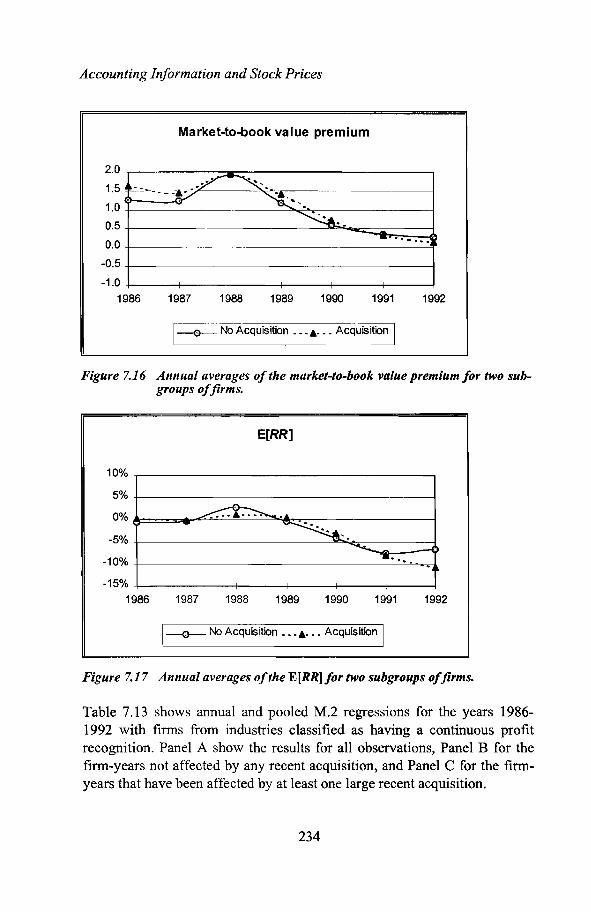
Accounting Information and Stock Prices
Market-to-book value premium
199219911990198919881987
2.0 -r------- ------------.....,1.5 T-----..----=-::-*--..-~---~~.____----------I
1.0 +------------..3Ilo,~.__--------1
0.5 +---------------==--..........------1
0.0 +---------------------=r
-0.5 -+-----------------------1
-1.0 +-----+-----t------i---+------+---~1986
[-----0--- No Acquisition ••••.•• Acquisition I
Figure 7.16 Annual averages ofthe market-to-book value premium/or two subgroups offirms.
E[RR]
10%
50/0
0%
-5°J'o
-10°J'o
-15%1986 1987 1988 1989 1990 1991 1992
1-----0--- No Acquisition ••••••• Acquisition I
Figure 7.17 Annual averages ofthe E [RR] for two subgroups 0/firms.
Table 7.13 shows annual and pooled M.2 regressions for the years 19861992 with firms from industries classified as having a continuous profitrecognition. Panel A show the results for all observations, Panel B for thefirm-years not affected by any recent acquisition, and Panel C for the firmyears that have been affected by at least one large recent acquisition.
234

Empirical Results: The Level Approach
Table 7.13 Annual M.2 regression results for the period 1986-1992 usingobservations from industries with continuous profit recognition.
P IA Allfiane : lrm-years
YEAR a PI P2 ]i2 n
1986 0.41 (2.1)* 3.82 (3.6)** 1.83 (5.6)** 27.9% 1061987 0.70 (3.1)** 1.68 (1.3) 1.20 (3.1)** 8.6% 1071988 1.17 (2.7)** -1.21 (-0.5) 1.54 (2.1)* 2.6% 1041989 0.23 (0.8) 1.86 (1.2) 2.06 (3.9)** 13.0% 1021990 -0.83 (-2.9)** 1.91 (1.5) 3.03 (6.3)** 30.9% 921991 -0.63 (-2.2)* 5.64 (5.1)** 2.73 (6.3)** 55.2% 741992 -0.47 (-1.8)* 3.39 (3.2)** 1.86 (5.0)** 46.2% 67
Mean 0.08 2.44 2.04 26.3% 93Pooled 0.18 (l.5) 4.29 (7.8)** 1.95 (9.8)** 20.6% 652
tt f~ t d bane : lrm-years no a ec e .y any recen acqulsl Ions
YEAR a PI /32 ]i2 n1986 0.63 (2.7)** 6.83 (4.9)** 1.34 (3.3)** 33.8% 751987 0.73 (2.6)* 4.48 (2.2)* 1.05 (2.1)* 11.3% 651988 1.12 (l.8) 4.37 (1.1) 1.39 (1.3) 1.0% 581989 -0.17 (-0.5) 5.22 (3.0)** 2.64 (5.0)** 40.4% 481990 -0.80 (-2.9)** 6.53 (4.3)** 3.11 (7.5)** 67.6% 431991 -0.76 (-2.3)* 6.26 (4.2)** 3.08 (6.6)** 71.0% 411992 -0.77 (-2.8)** 4.01 (2.9)** 2.46 (6.4)** 66.9% 39Mean 0.00 5.39 2.15 41.7% 53Pooled 0.20 0.4)** 7.35 (9.4)*· 1.97 (8.4)** 32.7% 369
tf~ t d btl tane : Irm-years a ec e lya eas one recen acquisl Ion
YEAR a PI /32 li. 2 n1986 0.42 (1.1) 1.08 (0.6) 2.01 (3.5)** 25.4% 311987 0.66 (1.8) -0.85 (-0.5) 1.40 (2.3)* 8.0% 421988 0.85 (1.6) -6.59 (-2.6) 2.20 (2.5)** 18.4% 46
i1989 0.83 (l.5) -1.13 (-0.5) 1.15 (1.2) -0.7% 541990 -0.30 (-0.5) -1.18 (-0.7) 2.02 (1.8)* 3.9% 491991 0.21 (0.4) 4.80 (3.0)** 0.96 (1.0) 21.0% 331992 0.62 (1.3) 3.92 (2.6)** -0.13 (-0.2) 18.6% 28
Mean 0.47 0.01 1.37 13.50/0 40Pooled 0.27 0.4) 1.63 (2.1)* 1.73 (5.0)·· 9.2% 283
t-statistics in parenthesis, a two-sided test is used for intercepts and a one-sided test for theslope coefficients.
* Significant at 0.0 1 ~ a ~ 0.05** Significant at a ~ 0.01
235

Accounting Inforn1ation and Stock Prices
The 'no acquisition group' shows more than three times as high ]i2 as compared to the 'acquisition group', both as a mean of annual regressions and inthe pooled regressions (41.7% vs. 13.5%, and 32.7% vs. 9.2% respectively).PI is non-significant for the 'acquisition group' for the years 1986-90 andeven shows the wrong sign for four years. In the 'no acquisition group' thePI estimates are much more stable (between 4.01 and 6.83) and more oftensignificant.
The results indicate that the use of E[RR] to explain the market-to-bookvalue premium for a group of firms that recently have made large acquisitions is very limited. This result may have several causes, such as the increased complexity of the organization after an acquisition implying increased uncertainty, the diverse treatment of acquired goodwill,26 or simplythe use of a poor estimation procedure ofE[RR].
One can suspect that the mechanical, historical performance based ROEprediction procedure used in this study is particularly inferior to, for example, analysts forecasts for firms that have recently made a large acquisition.The analyst can supposedly make adjustments related to differences ingoodwill treatment, 'odd accounting' for restructuring expenses, expectedsynergy gains, and so forth.
The regression results presented in table 7.14 provide some evidence regarding this matter. Regressions using earnings forecasts taken fromAffarsvarlden (the business weekly) is contrasted to regressions using thehistorical ROE-based prediction approach for the small group ofcompanies.27 The sample has again been grouped according to acquisitionactivity.
26 The goodwill issue will be addressed in the next section.27 See appendix T for details about this sample and the utilized earnings prediction
approach.
236

Empirical Results: The Level Approach
Table 7.14 Pooled M.2 regressions for a small sample of companies.
P IA E[ROE] b dane : ase on prevIous year s per ormance
1986-92 a PI P2 ]i2 nAll observations -0.44 (-3.0)** 6.71 (6.0)** 2.33 (13.8)·· 74.6% 112
No Acquisition -0.59 (-3.1)** 5.42 (3.3)** 2.57 (13.1)** 83.1% 60Acquisitions 0.41 (1.4) 7.28 (5.3)** 0.91 (2.2)* 39.5% 52
Panel B: E[ROE] based on forecasts in Affarsvirlden
1986-92 a PI P2 li2 nAll observations 0.05 (0.4) 10.62 (10.7)·· 2.02 (14.2)*· 83.5% 112
No Acquisition -0.07 (-0.4) 10.45 (7.0)** 2.18 (12.8)** 89.2% 60Acquisitions 0.70 (2.8)** 10.02 (7.9)** 0.94 (2.7)** 57.9% 52
t-statistics in parenthesis, a two-sided test is used for intercepts and a one-sided test for theslope coefficients.
* Significant at 0.01 ~ a ~ 0.05** Significant at a ~ 0.01
The explanatory power is larger in all cases using Affarsvarlden's forecasts.However, a reduced explanatory power for the acquisition group is presentilTespective of earnings prediction approach. The relative reduction appears,however, to be larger when using a current performance based ROEprediction. The first observation is consistent with the hypothesis thatacquisition intensive firms are more complex or difficult to value, the second observation is consistent with increased inferiority of the mechanicalprediction approach for firms growing by acquisitions.
It is further notable that the jJ 2 coefficient is lower for the acquisition group,irrespective of earnings prediction approach. The P2 coefficient is alsolower and often non-significant for the acquisition group in the annual regressions presented in table 7.13. The PMB calculations in this study havebeen based on an assumption that the firm holds an age-balanced portfolioof their particular combination of assets, and that intangible assets are notcapitalized. It was argued in Section 5.3.2 that a company that grows vialarge acquisitions reduces the measurement bias at least temporarily, as acquired tangible assets are revalued to present acquisition cost and acquiredintangible assets are capitalized. It is thus reasonable that the PMB losesdiscriminating ability-being less often significant-and shows a lower
237

Accounting Information and Stock Prices
regression coefficient for the acquiring group of firms. In the extreme case,when the acquired company is much larger than the acquirer, the PMBshould be expected to lose all discriminating ability.
7.4.2.1 Goodwill treatment method
The diverse accounting treatment of goodwill during the acquisition-intensive period 1986 to 1990 can be one explanation for the weak explanatorypower for the acquiring firms.28 This question is possible to study if theacquiring firms are divided into different 'goodwill treatment' groups. Twosuch groups have been specified: i) a (goodwill write-offgroup '- where atleast one large goodwill write-off has been done during the last or anyprevious period, and ii) a (no goodwill write-off group '-where no suchlarge goodwill write-offs has been done.29 The sample of all firms with acontinuous profit recognition has been used.
One effect of a writing off goodwill directly against equity is a reducedbook value of equity and an increased ROE.30 To investigate whether anysuch systematic differences can be observed in this study, figures 7.18, 7.19and 7.20 are presented. These figures show the annual means of the marketto-book value premiums, the E[RR] and the PMBs for the firms that have recently made a large acquisition, grouped according to their method ofgoodwill treatment.31
28
29
30
31
Between 1986 and 1990 a number of firms chose to write off goodwill directly againstequity.Firm-years have been assigned to the goodwill write-off group if a large goodwillwrite-off has been done during the last period or during any previous period. See detailsregarding the identification procedure of goodwill write-off firms in Section 5.3.2.Ceteris paribus, this will be the case for several years after the actual goodwill writeoff. If the 'vrite-off is included in the income statement, the actual write-off year will, ofcourse, look different.Note that the number of goodwill write-off firms is relatively small. The means arebased on between 7 and 13 observations each year.
238

Empirical Results: The Level Approach
Market-to-book value premium
199219911990198919881987
2.0 -r-------~~-----------_,
1.5 "'F-------'=--=~<----------='--...---------__t
1.0 +-----------------"~........------___I
0.5 +---------------~.:::__----~__f
0.0 -I-------------------------:y
-0.5 -1---------------------___1
-1.0 -+-----t------+----+------+-----t--~1986
1---0-- No GW write-off ••••••• GW w rite-off I
Figure 7.18 The average nlarket-to-book value premium for the acquisitionintensive firms, grouped according to the chosen method ofgoodwilltreatment.
E[RR]
100/0 -r-----------------------,50/0 -1-------------------------1.....•......0% ~--;;;;;;;;;;;;;;;;;;r.~-=.=---~\:J===~_(• •~.:::::::-._---._-_•.=.~.~------t
-50/0 +-------------..=...3Ioooo;;:--~........------1
-10% -I-------------------=--=:----.
199219911990198919881987-15% -+-----+-----+----+-----+-----+-----1
1986
1---0-- No GW write-off _...... GW w rite-off I
Figure 7.19 The average E[RR] for the acquisition-intensive firms, groupedaccording to the chosen method ofgoodwill treatment.
239

Accounting Information and Stock Prices
PMB
1.00 __------------------_
0.75 +------:-------------------1....... . -.•..... -.......0.50(~~ :; = ··--·t·······~·-·-·-·~~
0.25 -1---------------------1
1992199119901989198819870.00 -1----+-----+-----+---+-----+---......
1986
I--e------ f\b GW write-off - - -.- - - GW w rite-off I
Figure 7.20 The average PMB for the acquisition-intensive firms, groupedaccording to the chosen method ofgoodwill treatment.
The mean n1arket-to-book value premiums are practically identical for thetwo groups, whereas a consistent difference is evident concerning the meanvalues of E[RR]. The mean E[RR] is approximately 3 percentage pointshigher for the goodwill write-off firms.32 Simultaneously, a significant butdiminishing difference in the measurement bias appears to be present. Theearly write-off firms show a slightly higher average PMB.
In table 7.15 regression results for pooled 1986-92 data, grouped accordingto the goodwill treatment method are provided.
32 The mean difference is significant at the 5 percent level, as a total over the years between 1987 to 1992, but not for each individual year.
240

Empirical Results: The Level Approach
Table 7.15 Pooled M.2 regression results for the period 1986-1992 usingobservations from industries with continuous profit recognitionand firm-years affected by at least one recent acquisition.
1986-92 a PI PZ liZ nAll observations 0.27 (1,4) 1.63 (2,1)* 1.73 (5,0)** 9.2% 283
No goodwill write-off -0.07 (-0,3) 0.76 (0,9) 2.43 (5,2)** 10.2% 225Goodwill write-off 0.78 (3,4)** 7.16 (6,3)** 0.72 (2,2)* 42.7% 58
t-statistics in parenthesis, a two-sided test is used for intercepts and a one-sided test for theslope coefficients.
* Significant at 0.01 ~ a ~ 0.05** Significant at a ~ 0.01
Interestingly, a strongly significant PI coefficient amounting to 7.16 isshowed for the goodwill write-off group, whereas the group of acquiringfirms not writing off any goodwill, shows a non-significant PI coefficientamounting to 0.76. Furthermore, the adjusted explanatory power of the regression is 42.7% vs. 10.2%, in favor of the group of goodwill write-offfirms.
A priori, the capitalization of goodwill can be expected to be a more descriptive accounting valuation principle. Nevertheless, the level of ROEappears to have a very limited ability to explain the market-to-book valuepremium for the average acquiring firm with capitalized goodwill. A lack ofconfidence among investors regarding the substance of goodwill values andthe economic meaning of goodwill depreciation can be one explanation forthese results. Recall that the diversity of goodwill accounting during theperiod led many stock markets analysts (including Affarsvarlden, the business weekly) to exclude all goodwill in their calculations.
7.4.2.2 The poolilzg versus the purchase methodIt was previously argued that the consolidation method called 'par'(~'pooling'), the dominant method for Swedish groups until the mid 1970s,was in principle equivalent to the 'purchase method' with an imn1ediatewrite-off of purchased goodwill. In figures 7.18, 7.19 and 7.20 a systematicdifference in the mean level and the E[RR] and PMB (but not for themarket-to-book value premium), were observed for the two groups of firms
241
9 Runsten

Accounting Inforlnation and Stock Prices
choosing different goodwill accounting methods. To check if similar differences can be observed related to the chosen consolidation method, comparable figures have been constructed.33
Market-to-book value premium1.0 ...--------- --,
0.5 -1-----------------------1
-0.5 -1-----------------------1
197619751974197319721971-1.0 +-------+----t-----+-----+---+---....-o1
1970
E·.. Fboling rrethod~ F\Jrchase rrethod I
Figure 7.21 The average market-to-book value premium for firms groupedaccording to the chosen method ofconsolidation.
33 The main period of transition to the purchase method took place between 1970 and1976. The sample of firms with continuous profit recognition has been used.
242

Empirical Results: The Level Approach
E[RR]
10%
5%
0%
-5%
-10%1970 1971 1972 1973 1974 1975 1976
I·· .•... Fboling rrethod -----0-- RJrchase rrethod I
Figure 7.22 The average EIRR] for firms grouped according to the chosenmethod ofconsolidation.
PMB
1.00 ...,.....-------- .....,
0.75(~-w----G-)---_-9-__-D.-~-~-'-"'D_~~.A0.50 .......•....... i.. · . - .•.•... · ... II· •••••• ill· • • •• ~ I
0.25 +----------------------1
1976197519741973197219710.00 -+-----+------+-------l---+-----+------t
1970
E·..FOoling rrethod -----0-- RJrchase rrethod I
Figure 7.23 The average PMB for firms grouped according to the chosenmethod ofconsolidation.
A similar but weaker pattern can be observed as compared with the previousgoodwill write-off issue. The mean market-to-book value premium cannotbe separated between the two groups, whereas the mean E[RR] appears to be
243

Accounting Information and Stock Prices
higher for the pooling method firms.34 The firms that adapt to the purchasemethod earliest appear to have a somewhat higher mean PMB.
Table 7.16 shows annual and pooled regression results for 1970-76, with thesample of companies grouped according to chosen consolidation method.
Table 7.16 Annual M.2 regression results for observations from industrieswith continuous profit recognition.
rd fth ddtP rP IAane : 00 In~ me 0 use or conso 1 a Ion.
YEAR a /31 /32 li 2 n1970 -0.44 (-3.3)** 2.96 (2.4)* 0.48 (2.6)* 45.1% 181971 -0.03 (-0.3) 12.26 (7.5)** 0.88 (6.1)** 76.8% 231972 -0.09 (-0.7) 6.13 (3.2)** 0.54 (2.7)** 36.8% 231973 -0.49 (-3.7)** 4.15 (3.6)** 0.86 (4.3)** 55.5% 201974 -0.23 (-2.0) -1.25 (-1.3) 0.23 (1.4) 7.9% 171975 -0.09 (-0.7) 4.90 (2.9)** 0.38 (2.1)* 40.8% 161976 -0.12 (-1.0) 7.88 (4.7)** 0.61 (3.5)** 73.3% 11
Mean -0.21 5.29 0.57 48.0% 18Pooled -0.29 (-5.3)** 2.81 (5.0)** 0.51 (5.9)·· 30.6% 128
Panel B: Purchase method used for consolidation.
YEAR a /31 /32 Ii.2 n
1970 -0.41 (-1.7) 2.20 (0.5) 0.38 (2.0)* 17.1% 111971 0.39 (1.7) 15.05 (4.5)** 0.56 (3.0)** 66.5% 141972 0.18 (0.8) 8.22 (2.7)** 0.22 (1.1) 32.9% 161973 -0.11 (-0.7) 2.01 (1.1) 0.18 (0.8) 1.6% 201974 -0.15 (-0.9) -0.40 (-0.4) 0.07 (0.3) -8.5% 231975 -0.17 (-1.3) 3.49 (2.9)** 0.34 (1.9)* 32.2% 231976 -0.17 (-1.3) 3.24 (2.7)** 0.25 (1.5) 22.3% 30
Mean -0.06 4.83 0.29 23.4% 20Pooled -0.25 (-4.1)** 1.60 (3.1)** 0.29 (3.6)•• 13.4% 137
I-statistics in parenthesis, a two-sided test is used for intercepts and a one-sided test for theslope coefficients.
* Significant at 0.01 ~ a ~ 0.05** Significant at a ~ 0.01
Higher explal1atory power and more significant PI and P2 coefficients canbe observed every year for the group of pooling method firms. The P2 coefficient is particularly low for the group ofpurchase method firms.
34 The mean difference, however, is not statistically significant at the 5 percent level.
244

Empirical Results: The Level Approach
It should be noted that the main transition period of accounting method forconsolidation coincides with the transition period to open disclosure of economic value and depreciation of tangible assets. Attempting to control fordifferences in such accounting, all firm-years with non-open depreciationaccounting were eliminated. However, this control eliminated almost allpooling method observations (only eight firm-years remained). This indicates that the companies that were late in adapting to the purchase methodwere also late adapters to new disclosure practice regarding depreciation.This in tum implies that the higher explanatory power observed for thepooling method firms is not driven by more informative depreciationaccounting.
7.4.3 Accounting for associated companiesA gradual transition from the cost method to the equity method when accounting for associated companies took place during the 1980s for firnlslisted on the Stockholm Stock Exchange. The sample has been divided intotwo groups; i) firms USillg the equity method, and ii) firms using the costmethod (but providing the share of the associated company's earnings in thenotes). The sample of firms with a continuous profit recognition have beenused.
1985 to 1987 is the only period when about ten different firms used the twomethods simultaneously. TIle opportunities for statistical analysis are therefore very limited,35 but two efforts have, nevertheless, been attempted. First,pooled M.2 regression results for the period 1985 to 1987, with the samplegrouped according to accounting method for associated companies, are provided in table 7.17. Secondly, M.2 regression results with firm-years clustered around the actual switch year in accounting method are provided intable 7.18.
35 Appendix V illustrates the mean value of the dependent and the independent variables,grouped according to different accounting methods for associated companies.
245

Accounting Information and Stock Prices
Table 7.17 Pooled M.2 regressions for companies using the cost method versus companies using the equity method. Data for the period 198587 with companies from industries with continuous profit recognition have been used.
1985-87 IX PI P2 li2 n
All companies 0.50 (4.3)** 3.70 (5.2)** 1.34 (6.9)** 19.1% 314Cost method 0.74 (2.7)** 4.16 (2.8)** -0.22 (-0.5) 16.6% 31
Equity method -0.01 (-0.0) 0.28 (0.1) 1.72 (2.6)** 13.5% 36
t-statistics in parenthesis, a two-sided test is used for intercepts and a one-sided test for theslope coefficients.
• Significant at 0.01 ~ a ~ 0.05•• Significant at a :::; 0.01
Table 7.18 M.2 regressions for companies switching from the cost method tothe equity method. Data for the period 1980-93 and companiesfrom industries with continuous profit recognition have been used.
IX PI P2 li2 n
2 years before switch 0.81 (1.7) 6.21 (3.1)** -0.22 (-0.3) 35.2% 151 year before switch 0.64 (1.3) 5.84 (3.0)** 0.24 (0.3) 36.7% 15
Switch year 1.27 (2.1) 4.86 (1.4) -0.94 (-1.0) 1.9% 151 year after switch 0.91 (1.5) 4.74 (1.1) -0.70 (-0.7) -3.4% 12
2 years after switch 0.60 (1.0) 8.87 (1.9)* 0.49 (0.5) 15.1% 11
t-statistics in parenthesis, a two-sided test is used for intercepts and a one-sided test for theslope coefficients.
• Significant at 0.01 :::; a :::; 0.05•• Significant at a:::; 0.01
The regression results appear to indicate that the E[RR] variable is particularly weak as an explanatory variable of the market-to-book value premiumfor firms using or switching to the equity method. However, given the limited sample size, this indication should be interpreted very cautiously.
246

8 EMPIRICAL RESULTS: THE CHANGE
ApPROACH
As a first step, changes in market prices have been explained by the growthin accounting equity on its own, utilizing regression specification M.3. As inEaston, Harris and Ohlson (1992) and Ohlson and Penman (1992), thestudied value change window has successively been increased from a oneyear period, to a value change window of ten years. The regressions havebeen estimated for each possible individual period. For windows exceedingone year, the value change window has been moved forward one year at atime. This means that for a value creation period of two years, the period1967 to 1969 has been estimated first,1 then the period 1968 to 1970, and soforth. This means that the number of different regressions has been 26 atnlost for the one-year tinle interval and 16 for the ten-year time interval. Theone-year value change regressions have also been estimated in pooled crosssection and time-series. Note that a pooled regression using both crosssectional and time-series data for the longer periods (two years or more)would overexploit the data (given the time overlap approach).2
To be precise, recall that the value change is actually measured, in this example, between the end of March 1968 and the end of March 1970.
2 For general statistical considerations see appendix R.

Accounting Information and Stock Prices
8.1 Regression model M.3
M.3 Pj,t+k - Pj,t=a+c1
Pj,t
b. k -b.J,t+ J,t f'"Oo.J
+ Gj,t+kPj,t
In table 8.1 the annual one-year value change regression results for the fullsample of finns are reported.3 The slope coefficients (el) had the expectedpositive sign in all annual regressions. The average coefficient was 0.56 andvaried between 0.15 and 1.48 in the 26 regressions. In 18 of the 26 annualregressions, the change in book value of equity variable had a significantexplanatory power of the change in market value (on at least the 5 percentlevel). The pooled regression generated a highly significant slope coefficientof 0.77 (t-statistic = 13.7) and an explanatory power of 7.4%. The averageexplanatory power (R2) of the annual regressions was 8.7%. The change inbook value of equity (retained value creation) thus explained only a smallpart of the value change observed in the stock market. For some years, 1969to 1972, 1980, 1987 and 1993, the change in equity hardly explained any ofthe market price changes.
3 In order to reduce the potential effect of a few extreme observations the following truncation rule has been utilized: exclude observations (firm-years) if either
Pj,t+k - Pj,t >i) mean(l1p) ± 3· a(l1p)
Pj,t <b. k-b. >
ii) J,t+ J,t mean (l1b) ±3. u(l1b)Pj,t <
...) [Et+k(R~,t+k+l) - Et(~,t+l)l>111 - mean(ARI) ±3· u(MU)
Pj,t <The means and standard deviations of each variable, for each period length have beenpresented in section 6.1. The use of this truncation rule somewhat reduces the overallexplanatory power of the regressions, but beyond that, seems to only marginally affectthe regression coefficients.
248

Table 8.1
Empirical Results: The Change Approach
Annual one-year M.3 value change regressions for the full sampleof firms.
YEAR d el R2 n1968 0.34 (8.0)** 0.90 (3.4)** 24.1% 381969 -0.18 (-5.0)** 0.27 (0.9) 2.1% 381970 -0.06 (-1.5) 0.18 (0.6) 1.0% 411971 0.24 (4.5)** 0.21 (0.7) 1.2% 421972 0.09 (3.7)** 0.15 (1.0) 1.5% 681973 0.09 (3.0)** 0.77 (4.2)** 20.5% 711974 -0.04 (-0.1) 0.27 (2.0)* 5.2% 731975 0.16 (4.0)** 0.89 (4.1)** 20.0% 681976 -0.03 (-1.0) 0.33 (2.2)* 6.0% 751977 -0.19 (-9.0)** 0.39 (3.0)** 10.9% 771978 0.04 (1.3) 0.48 (2.5)** 7.7% 791979 0.07 (2.3)** 0.49 (3.3)** 12.3% 781980 0.37 (8.2)** 0.19 (1.0) 0.7% 831981 0.29 (7.4)** 0.38 (2.0)* 4.4% 851982 0.71 (13.5)** 0.99 (3.6)** 14.5% 771983 0.39 (7.9)** 0.61 (1.6) 2.9% 891984 -0.23 (-9.5)** 0.36 (2.1)* 4.6% 911985 0.23 (6.5)** 0.59 (2.0)* 2.7% 1431986 0.41 (10.5)** 0.90 (3.2)** 6.8% 1461987 0.12 (4.6)** 0.39 (1.5) 1.4% 1531988 0.29 (9.3)** 1.48 (5.4)** 16.4% 1501989 -0.03 (-1.0) 0.93 (3.5)** 7.1% 1581990 -0.27 (-12.5)** 0.61 (3.7)** 9.1% 1381991 -0.24 (-7.6)** 0.82 (4.9)** 16.1% 1251992 -0.07 (-2.5) 0.74 (5.6)** 22.2% 971993 0.62 (12.4)** 0.36 (l.5) 1.5% 80
Mean 0.12 0.56 8.7% 91Pooled 0.11 (12.0)** 0.77 03.7)** 7.4% 2363
t-statistics in parenthesis, a two-sided test is used for intercepts and a one-sided test for theslope coefficients.* Significant at 0.01 ::; a ::; 0.05** Significant at a ::; 0.01
Very similar overall regression results have been presented in Easton andHarris (1991) and Ohlson and Penman (1992), both using US data for theperiods 1968-86 and 1970-87 respectively (see table 8.2).4
4 Note that the regression specification used in Easton and Harris (1991) includeddividends paid in the dependent and independent variable. Thus they explained totalreturn using accounting earnings (normalized with opening period stock price). In spiteof this difference, the results are remarkably similar.
249

Accounting Information and Stock Prices
Table 8.2 One-year M.3 value change regression results of this study compared to results presented in Easton and Harris (1991) and Ohlson and Penman (1992).
Proportion ofStudy tl el R2 n significant el years
a ~ 0.05Mean ofannualregressionsEaston & HarrisA 0.08 1.02 10.5% 1,052 100.0%Ohlson & PenmanB 0.07 0.87 11.0% 1,600 n.a.Runsten 0.12 0.56 8.7% 91 69.2%
'Pooled regressionsEaston & HarrisA 0.11 (30.8)** 0.82 (40.3)** 7.5% 19,996Runsten 0.11 (12.0)** 0.77 (13.7)** 7.4% 2,363
I-statistics in parenthesis, a two-sided test is used for intercepts and a one-sided test for theslope coefficients.* Significant at 0.01 ~ a. ~ 0.05** Significant at a. ~ 0.01
A) Calculated from Levels model results in table 1, Easton and Harris (1991).B) From panel A in table 1, Ohlson and Penman (1992).
As is evident fron1 the table, the pooled regression result in this study waspractically identical to the result in Easton and Harris (1991), both in termsof explanatory power and regression coefficients. In terms of the means ofrepeated annual regressions, the present study on Swedish data showed alower estimate of the slope coefficient and a slightly lower R2. The moststriking difference, however, concerns the relative frequency of significantel coefficients. In Easton and Harris (1991), annual earnings provided asignificant explanation of returns in all annual regressions, whereas in thepresent study this was the case in only 69% of the years. Given the overallrather low explanatory power in both studies, this difference can probablybe attributed to the large difference in sample sizes (91 observations peryear in this study as cOlnpared to 1,052 in Easton and Harris).
In table 8.3, M.3 regressions with successively increased time intervals arepresented. The average explanatory power of the regressions showed amonotonous increase from 8.7% for the one-year time interval to 35.4% for
250

Empirical Results: The Change Approach
the ten-year time interval. For the two-year time interval regressions thechange in accounting equity had a significant explanatory power in 21 of the25 regressions. For the five- and ten-year intervals, all individualregressions were significant.
Table 8.3 The mean of repeated M.3 value change regressions for differentintervals for the full sample.
Proportion ofTime interval a e1 R2 n significant el years
(Year) a. ~ 0.05
1 0.12 0.56 8.7% 91 69.2%2 0.20 0.75 12.5% 85 88.0%5 0.52 1.03 26.6% 67 100.0%
10 1.43 1.32 35.4% 46 100.0%
Again, it is notable how similar these results are to those presented inOhlson and Penman (1992). The mean R2 in their study followed theincreasing pattern 11%, 16%, 29% and 43%, for the same time intervals.Furthermore, Easton, Harris and Ohlson (1992) in a similar study using USdata for the period 1968-86 showed a R2 pattern increasing from 6%, 15%,33% to 63%. Also O'Hanlon and Pope (1997) using UK data show resultsthat are consistent with increasing explanatory ability of earnings as thetime interval studied is prolonged.5 These results are all in line with thehypothesis that value creation is described with less error for a longer timeinterval. Easton, Harris and Ohlson drew the following conclusion:
HThe idea of a correlation increase as the return interval increases stems from an application ofaccounting concepts. Thatis, earnings aggregate over periods, so that earnings are morelikely to reflect the value-relevant events and their effect onvalue changes over longer periods. This framework naturallyleads to the conclusion that investors 'buy earnings '. "
Easton, Harris and Ohlson (1992, p. 140)
According to the simple assumptions behind M.3, a unit of recognized valuecreation according to the accounting convention is expected to be translated
5 The mean R2 in their study followed the pattern 14%,23%, 41%, 40% and 65%, forthe time intervals, 1, 2, 5, 10 and 20 years.
251

Accounting Information and Stock Prices
into a unit of value creation in market value terms (implying that the elcoefficient should equal 1.0). From the table above, one may conclude thatthe el coefficients successively increase when the time interval is lengthened. For the ten-year period, it actually exceeded 1.0 (1.32 as a mean ofrepeated regressions). A similar pattern has been noticed both in Easton,Harris and Ohlson (1992) and in Ohlson and Penman (1992).
"A dollar of earnings evidently is associated with more than adollar ofchange in value for long return periods. "
Easton, Harris and Ohlson (1992, p.139)
Ibid. further noticed that they have no easy and direct explanation as to whythis pattern occurs. O'Hanlon and Pope (1997) received slope coefficientsthat fluctuated around 2.0 for both short and long intervals. According to thevaluation model outlined in this study (see Chapter 2), the el coefficient isexpected to equal 1.0 only if the firms studied are not expected to have apermanent measurement bias. Given the mixed sample of firms in thisstudy, a el coefficient exceeding 1.0 is thus not unexpected. (Inclusion ofcontrol for different expected levels of PMBs will be evaluated withregression specification M.5 later.) Also note that the total mean of theannual median market-to-book value premiums of the firms included in thisstudy was 0.38 (see table 6.1). Table 6.1, also shows a systematic change inthe market-to-book value premium over time. The market-to-book valuepremium was consistently lower during the first half of the period studied(1967 to 1980). This systematic change is likely to influence the estimatede1 coefficient (and probably also the intercept, tl) in the long windowregressions, given the simple specification ofM.3.
There are several possible reasons behind a general change in market-tobook value premiums: i) changed accounting principles, ii) the effect of along period of high inflation, iii) the median firm investing on average morein intangible assets, iv) a changed mix of business types represented on thestock exchange, v) generally changed business climate, and vi) new groupsof investors with other investment policies (i.e., institutional and international investors). Some of these sources will be controlled for in later sections, while others could ideally be picked up by time- and firm-specificcalculations of the expected PMB.
252
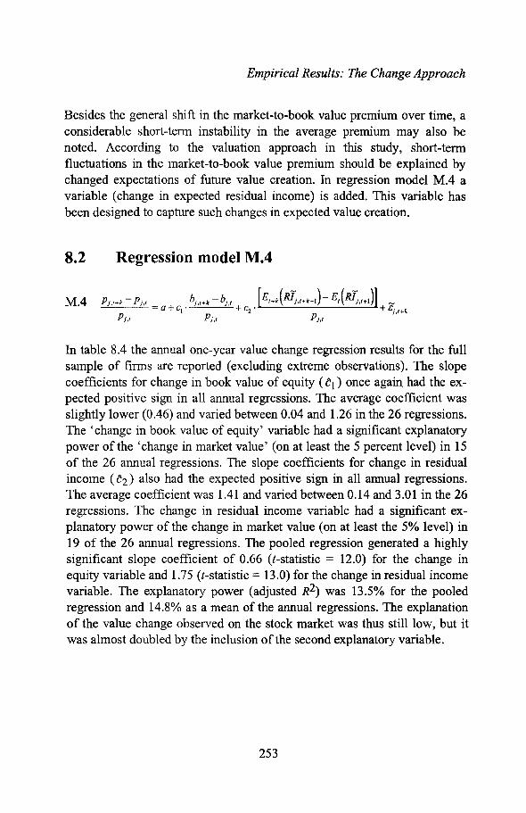
Elnpirical Results: The Change Approach
Besides the general shift in the market-to-book value premium over time, aconsiderable short-term instability in the average premium may also benoted. According to the valuation approach in this study, short-termfluctuations in the market-to-book value premiunl should be explained bychanged expectations of future value creation. In regression model M.4 avariable (change in expected residual income) is added. This variable hasbeen designed to capture such changes in expected value creation.
8.2
M.4
Regression model M.4
In table 8.4 the annual one-year value change regression results for the fullsample of firms are reported (excluding extreme observations). The slopecoefficients for change in book value of equity (el) once again, had the expected positive sign in all annual regressions. The average coefficient wasslightly lower (0.46) and varied between 0.04 and 1.26 in the 26 regressions.The 'change in book value of equity' variable had a significant explanatorypower of the 'change in market value' (on at least the 5 percent level) in 15of the 26 annual regressions. The slope coefficients for change in residualincome (e2) also had the expected positive sign in all annual regressions.The average coefficient was 1.41 and varied between 0.14 and 3.01 in the 26regressions. The change in residual income variable had a significant explanatory power of the change in market value (on at least the 5% level) in19 of the 26 annual regressions. The pooled regression generated a highlysignificant slope coefficient of 0.66 (t-statistic = 12.0) for the change inequity variable and 1.75 (t-statistic = 13.0) for the change in residual incomevariable. The explanatory power (adjusted R2) was 13.5% for the pooledregression and 14.8% as a mean of the annual regressions. The explanationof the value change observed on the stock market was thus still low, but itwas almost doubled by the inclusion of the second explanatory variable.
253

Accounting Information and Stock Prices
Table 8.4 Annual one-year M.4 value change regressions for the full sampleof firms.
YEAR tl e, e2 R2 n1968 0.31 (7.0)** 0.58 (1.8)* 1.74 (1.7) 25.7% 381969 -0.19 (-5.2)** 0.33 (1.1) 0.67 (1.3) 1.2% 38]970 -0.03 (-0.7) 0.04 (0.1) 0.75 (1.3) 0.4% 411971 0.33 (6.3)** 0.04 (0.1) 3.01 (3.9)** 24.8% 421972 0.07 (3.2)** 0.07 (0.5) 1.07 (2.1)** 4.8% 681973 -0.06 (-2.2)* 0.50 (3.0)** 1.70 (5.1)** 40.9% 711974 0.00 (-0.1) 0.15 (1.1) 0.68 (2.0)* 7.7% 731975 0.17 (3.5)** 0.87 (3.9)** 0.14 (0.3) 17.7% 681976 0.01 (0.4) 0.27 (1.9)* 1.42 (3.9)** 20.1% 751977 -0.14 (-5.6)** 0.44 (3.7)** 1.47 (4.2)** 26.0% 771978 0.01 (0.4) 0.47 (2.8)** 1.91 (5.0)** 28.6% 791979 0.07 (2.1)* 0.42 2.9)** 1.37 (2.6)** 17.4% 781980 0.38 (8.5** 0.29 (1.2) 1.00 (2.0)* 3.0% 831981 0.32 (8.4)** 0.28 (1.5) 1.75 (3.6)** 15.5% 851982 0.72 (14.0)** 0.95 (3.5)** 2.05 (2.4)* 18.3% 771983 0.39 (8.2)** 0.26 (0.6) 2.12 (2.4)* 6.7% 891984 -0.23 (-9.3)** 0.33 (1.9)* 0.23 (0.6) 2.9% 911985 0.26 (7.3)** 0.35 (1.2) 1.80 (3.4)** 9.0% 1431986 0.43 (11.2)** 0.53 (1.8)* 2.62 (3.4)** 12.5% 1461987 0.13 (5.2)** 0.18 (0.7) 1.89 (3.0)** 5.8% 1531988 0.29 (9.5)** 1.26 (4.4)** 1.41 (2.3)* 18.2% 1501989 -0.02 (-0.6) 0.85 (3.0)** 0.55 (0.9) 6.3% 1581990 -0.26 (-11.8)** 0.69 (4.2)** 1.29 (2.9)** 13.1% 1381991 -0.20 (-6.2)** 0.81 (4.9)** 1.61 (3.3)** 21.6% 1251992 -0.06 (-2.1)* 0.68 (4.8)** 0.61 (1.6) 23.3% 971993 0.53 (9.7)** 0.25 (1.1) 1.83 (3.2)** 12.0% 80Mean 0.12 0.46 1.41 14.8% 91Pooled 0.12 (13.7)** 0.66 (12.0)** 1.75 03.0)** 13.5% 2363
t-statistics in parenthesis, a two-sided test is used for intercepts and a one-sided test for theslope coefficients.* Significant at 0.01 ~ a ~ 0.05** Significant at a ~ 0.01
In table 8.5 the regression results of this study are compared to the resultspresented in Easton and Harris (1991).6 Their multiple regression model isquite similar to M.4,7 even if their motive for the regression specification
6
7
The regression results in Easton and Harris (1991) were generated from a large sampleof US firms for the period 1968 to 1986.The multiple regression model specified in Easton and Harris (1991) was as follows(Easton and Harris denoted earnings A rather than X):
254

Empirical Results: The Change Approach
differs from the one proposed in this study. They set out to test whethermarket return is best explained by 'accounting earnings' or 'change inaccounting earnings'-viewing the two variables more or less as competitors. In this study, 'change in equity' (earnings minus dividends) and'cllange in expected residual income', are viewed as two complementaryindicators, each explaining different aspects of value changes-value creation (retained) and changed expectations regarding the firm's ability tocreate value. The 'change in earnings' variable has long been used inmarket-based accounting research as an indicator of unexpected earnings.For example, the line of research that Lev (1989) evaluated, and expressedconcern about, used 'change in earnings' as the main explanatory variableof return in most cases.
Table 8.5 One-year M.4 value change regression results of this study compared to the results presented in Easton and Harris (1991).
Proportion ofStudy Ct el e2 ](2 n significant
el years eZ yearsa. ~ 0.05 a. ~ 0.05
Mean ofannualregressionsEaston & HarrisA 0.10 0.85 0.24 11.4% 1,052 100.0% 52.6%Runsten 0.12 0.46 1.41 14.8% 91 57.7% 73.1%
!RoofedEaston & HarrisA 0.12 (31.6)** 0.71 (28.3)** 0.16 (7.1)** 7.7% 19,996Runsten 0.12 (13.7)** 0.66 (12.0)** 1.75 (13.0)** 13.5% 2,363
I-statistics in parenthesis, a two-sided test is used for intercepts and a one-sided test for theslope coefficients.* Significant at 0.01 ~ a ~ 0.05** Significant at a ~ 0.01
A) Calculated from multiple regression model result in table 3, Easton and Harris (1991).
P · I+D. I-P·t X. I X. I-X.j,t+ j,t+ j, _ •~ • j,t+ j,t?lr'- a +cI +c2 + Gj,t+k
Pj,! Pj,t Pj"
The change in earnings variable equals the change in residual income variable if thefirm has no growth in equity and the cost of equity capital is a constant.
255

Accounting Information and Stock Prices
It is noteworthy that Easton and Harris showed weaker results concerningthe complementarity of the two explanatory variables than those found inthe present study.8 The overall explanatory power did not increase as much,and the 'change in earnings' variable was not as often significant, despitethe much larger US sample. Easton and Harris did, nevertheless, reach thefollowing conclusion:
((Overall, the evidence suggests that both the current earningslevels variable (Ajt/Pjt-I) and the earnings changes variable(Mjt/P·t-i) are relevant for explaining returns, and the twovarzables are not just substitutes. They are complements in thesense that, for the pooled sample and several individual years,significantly more cross-sectional variation in returns is explained by both earnings levels and earnings changes than is explained by either variable considered alone "
Easton and Harris (1991, p. 31)
The main difference in regression results, besides the slightly less frequentsignificance of the 'change in earnings' variable, concerns this variable'sestimated slope coefficient. The slope coefficient of the pooled and themean of annual regressions were only 0.16 and 0.24 respectively, ascompared to the 'change in residual income' variable with regressioncoefficients amounting to 1.75 and 1.41 respectively. The slope coefficientof M.4 can be given an economic interpretation, given the proposedvaluation framework of this study. The slope coefficient can be viewed asan indicator of the expected permanence of the 'new performance level'.According to the discussion in Chapter 2, a GPF amounting to 1 indicatesno pennanence and a GPF exceeding, for example, 10 indicates strongexpected permanence of the new performance level, possibly combined withexpected growth. The slope coefficient of the 'change in earnings' variablehas been given a similar economic interpretation in 'the market-basedaccounting research literature; it has often been called the 'EarningsResponse Coefficient' (ERe). A rather low estimated ERC is a wellrecognized phel10mena. A plausible explanation for this observation wasprovided in Ali and Zarowin (1992):
8 Recall that the utilized earnings change variables are not identical. Likely consequencesof this fact will be further developed below.
256

Empirical Results: The Change Approach
"In the presence oftransitory components ofearnings, the previous period's earnings are a poor proxy for the current period'sexpected earnings and the change in earnings is a poor proxy forunexpected earnings. We show that using the change in earningsas a proxy for unexpected earnings causes earnings response coefficients (ERCs), the slope coefficients in regressions ofreturnson unexpected earnings, to be biased toward zero and is a potential reason for the widely documented, empirically low ·ERCs*) "
*) liAs Ball and Watts (1972) and Watts and Zimmerman (1986) point out, ifannual earnings follow a random walk, earnings response coefficients areexpected to be 1+ l/r, where r is the rate for discounting future earnings.Thus, for historiGally experienced discount rates ofabout 12%, earningsresponse coefficients are theoretically expected to be about 9; howeverthey are typically estimated at below 3. "
Ali and Zarowin (1992, p. 250)
The 'change in residual income' variable used in this study is, as such, acrude proxy for unexpected perforn1ance. It is, however, potentially 'richer'than the simple 'change in earnings' variable in three respects: i) it controlsfor growth in earnings which is merely associated with retained earnings(via growth in equity), ii) it controls for changes in the cost of equity capital,and iii) the effect of an extreme period of transitory earnings is reduced viathe utilized mean regression function (arctan). Together these differencesmay well be an important reason behind the higher coefficients in this study.A sample of heterogeneous firms that includes firms with low predictivevalidity of their historical ROE, such as the full sample in the present study,can also cause low slope coefficients. This possibility will be evaluated inforthcoming sections.
The results of running M.4 on longer time intervals are presented in table8.6. As observed regarding M.3, the 'change in equity' variable was increasingly significant for the longer windows. Its slope coefficient also increasedand on average exceeded one (1.40) for the longest window. The inclusionof the 'change in residual income' variable increased the explanatory powerof the regressions for all time intervals. The mean ]l2 more than doubled forthe two-year window. The smallest relative increase was shown for the tenyear interval-from 37.9% to 47.1%-but it was still a considerable rise.The coefficients significantly exceeded zero in most of the regressions, butnot all. The mean level of the slope coefficients (e2) also followed an in-
257

Accounting Information and Stock Prices
creasing pattern-from 1.41 for one-year value change regressions to 3.93for the ten-year interval. These higher values are more consistent with theestimated GPFs in the value level regressions in the previous chapter. Themean GPF coefficient for the full sample using M.2 was 4.03 (see table7.S).
~able 8.6 The mean of repeated M.4 value change regressions for differentintervals for the full sample.
Time interval Proportion of(Year) tl el e2 ](2 n significant
e1 years e2 yearsa. ~ 0.05 a. ~ 0.05
1 0.12 0.46 1.41 14.8% 91 57.7% 73.1%2 0.22 0.68 2.23 26.3% 85 92.0% 80.0%5 0.58 1.05 2.88 37.9% 67 100.0% 72.7%
10 1.70 1.40 3.93 47.1% 46 100.0% 70.6%
8.3
M.S
Regression model M.5
Pj,t+k - Pj,t bj,t+k -bj,t [Et+k(Rlj,t+k+l) - Et(Rlj,t+l)]=a+ct • +c2 , +
P~ P~ P~
(bj,t+k -bj,JPMBj _+ C3 • + &j,t+k
Pj,t
In regression specification M.S, a third explanatory variable is addedchange in book value of equity multiplied by the estimated industry specificPMB, divided by opening market value.9 This new variable will naturally behighly correlated with the 'change in book value of equity' variable. IO Thiscauses collinearity, and the economic interpretation of individual regressioncoefficients is therefore strongly impaired. A large positive el coefficientmay be combined with a large negative e3 coefficient, or vice versa.
9
10
Recall that the estimated PMEs in general are industry-specific, with the exception ofthe R&D intensive firms, for which firm specific estimates have been used.See discussion regarding multicollinearity in appendix R.
258

Empirical Results: The Change Approach
Furthermore, one individual variable's degree of significance is stronglyinfluenced by the other. 11
To avoid problems of multicollinearity without excluding the effect ofdifferent PMBs, the following regression model has been specified. Here themeasurement bias has been incorporated into the value creation variable.The slope coefficient e{ in M.5' is expected to equal 1.0, given validestimates of the measurement bias.
M.5'
P't+k - p. t (bj,t+k -bj,t ).(1+ PMBj )j, j, = a + c{ . +
Pj,t Pj,t
[Et+k(R!N+k+l) -Et(R!j,t+I)] _+ c2 • + Ej,t+k
Pj,t
Table 8.7 includes regression results for successively longer windows usingspecification M.5' .
Table 8.7 The mean of repeated M.5' value change regressions for differentintervals for the full sample.
Time interval Proportion of(Year) tt ei e2 ][2 n significant
ei years e2 yearsa ~ 0.05 a ~ 0.05
1 0.13 0.31 1.41 15.1% 91 65.4% 76.9%2 0.22 0.47 2.23 26.8% 85 88.0% 84.0%5 0.57 0.69 2.83 I 40.6% 67 100.0% 72.7%
10 1.74 0.86 3.59 53.5% 46 100.0% 64.7%
The new combined slope coefficient (e{) was significant as often as e1when using M.4 and the same data. 12 The mean coefficient increased from
11
12
The explanatory power can, however, still he interpreted. Regression results of M.5with increasing time intervals are not reported; it can be noted, however, that the mean][2 increased (compared to M.4) for all four intervals studied, with a more pronouncedeffect regarding the two longer intervals.All individual regressions were significant (at the 5 percent level) for the two longerintervals. In comparison to the M.4 specification, the coefficient was significant in onemore and one less regression respectively, when the one- and two-year changeregressions were run.
259

Accounting Information and Stock Prices
0.31,0.47,0.69 to 0.86 when the interval increased successively from 1 to10 years. For the shorter windows the mean explanatory power was onlymarginally higher as compared to the results using specification M.4-however, for the longest window the mean ](2 increased from 47.1% to53.5%, indicating that the PMB has sonle discriminating ability. Theincreasing explanatory power supports the hypothesis that firms aredifferent with respect to their degree of measurement bias and that theestimation procedure of this study captures some of these differences.Specification M.5' will be used as the main model in the forthcoming sections.
8.3.1 Stability in association over timeFrom the annual value change regressions ofM.3 and M.4 presented in table8.1 and 8.4 above, it is clear that the explanatory power of the tested regressions have been unstable over time. To create a visual illustration of how theexplanatory power of regression specification M.5' has changed over time,four graphs have been constructed. Figures 8.1a, b, c and d illustrate valuechange intervals of 1, 2, 5 and 10 years respectively.l3
13 dB(l+PMB) = the change in book value ofequity times (l+PMB) variabledRI = the change in expected residual income variable
260

Empirical Results: The Change Approach
Total and relative contribution to adjusted R2
80% -r-------------------------__.700/0 +----------------------------1
60°1'0500/0 +----------------------------1
40°1'0 +-------E+-------------------__f
30% +------..{:t----=~;______------------__f
20% -Hll~11t---t:]---..:::::t____i .....__I:~:f--I::::1:1t_------- r__-___[:;:;I___mJ___f
100/0 +-.----J111:t--__--I.-.~;8a_..__I___fi:J_--MI_ -____"'l____'~ I____--n.. ....m_I
0% ~+--r---I~~~__+A-+-...,..~~+__~f_Ia.+..IiIiIiII.+_~__+A~~~~+__~.._...
coco0'>
of"'0'>-r-
coco0)-r-
o0)0)
Figure 8.la The adjusted R2 per year of repeated one-year value change regressions (M. 5 J, for the full sample. The total R2 is sub-divided into therelative contribution from each ofthe two explanatory variables.
Total and relative contribution to adjusted R2
80% -r-----------------------------,700/0 +---------------------------t
600/0 +-----------------------------1
50% -1------[::::::1--....,.",."..------------------1
400/0 +-----f'll;ll--t:H---+,:,,]---=-----i':::l:,l---------------f:%H
30% +-----rm-----{;:;:;:I--F;t---r::,;l,I---rn-I;l,:a----I;~.::J_Il§;I_____f::::::t--------- -i~;H
200/0 -t-=--f;:;:;:t-----{;:;1;;I--f:,;;:t-."......,.- --f;1::,11-1,gl---1r:J:l--t;i::l---t~;I__--n:;l-n;:t---mt----liiiiiI"----tt+--I1~~t--i*iH
10% +-.--LiiiI--l;;:,:I--f:;,;:I-__--m;:I- .-IIiIt-I--.J~ I-III--I%;I____--I;@I-tiiI ____
0% -+--+-+--+---~~-----+--+--+--+-J-...,...--+---+---+-...,..L+--~~~~+-+---+---I~l!) f"'- 0'> ex; C") LO ,..... 0) ~ C")f"'- f"'- ,..... co ex:> ex:> ex:> 0) (J)0'> 0'> 0'> 0> (J) (J) 0) 0) 0> (J)~ ~ -r- ~ ~ ~
I_ dB(1+prrb) II dRi I
Figure 8.lb The adjusted R2 per period of repeated two-year value change regressions (M. 5 J, for the full sample. The years in the graphs relateto the end ofeach period.
261

Accounting Information and Stock Prices
Total and relative contribution to adjusted R2
800/070%60%50°1'040°1'030°1'020%
I10°1'000/0 I
C'\I -.::t co...... ...... ......0> 0> 0>~ ~
m1I II
I I ..0 C'\I
~(0 co 0 C'\Ico co co co 0> 0>
0> 0> 0> (J) 0) (J) 0)~ ~ ~ ~ "C"""
I_ dB(1 +prrb) II dRi I
Figure 8.Ic The adjusted R2 per period of repeated five-year value change regressions (M. 5 ), for the full sample. The years in the graphs relateto the end ofeach period.
Total and relative contribution to adjusted R2
I:I ~
~i: •I I II III I II II
('t') LO ...... (J) a; (W')co co co co (J)0> 0) 0) 0) 0) (J)
~ ~ ~ ~ ~
80°1'0 -r------------------------~700/0 +--l'41§l----m:;;;;;I---v:~n---,_-I';;~"iJ---------------__I
60% -+-I:;*:::::t-----t:::~;'::::I----n~:;;:I_____I!lr:;!l'l_-N;;;,I_-____, __I§.~;a__--------------i
50% -+-Il:;;:;;::t---;:;:::::::t---n'<~:::t---t,::::l,::;t--Il~*,l'l---m,~I----I :}-__t-----. -------~ .,
400/0 ~~i:;:::::;I__ ~ ----f;i;;;iii;ii-----l -----~l__lma___I~
30% ~----., I____II I__I --w iI---=-----EmII--liliIilill-__..
20°1'0 ~~ ~ ._..._, ._..._, ---1~ ...............~
10% ~ I____II I__I --. ---..t ~ H
0% +--1I....j-I--.;.---+--II....j-I--+----+o--II...+-I--+---+--II...+-I--+----+o--II...+-I--+..-.-o+--II...+-I-.....
I_ dB(1+prrb) IIiI dRi I
Figure 8.Id The adjusted R2 per period of repeated ten-year value change regressions (M. 5), for the full sample. The years in the graphs relateto the end ofeach period.
262

Empirical Results: The Change Approach
Each period's total adjusted R2 has further been sub-divided into the relativecontribution from each of the two explanatory variables (change in equitytimes (l+PMB) and change in expected residual income).14 The meancontribution to the adjusted R2 from each explanatory variable in therepeated regressions is presented in table 8.8.
Table 8.8 The mean adjusted R2 sub-divided into the relative contributionfrom each of the two explanatory variables, for different time intervals for the full sample, using regression specification M.5'.
Time interval Relative JI2 Relative JI2 Total ](2
(Year) tlb·(I+PMB) M[Rl]1 7.0% 8.1% 15.1%2 11.7% 15.2% 26.8%5 25.6% 15.0% 40.6%
10 37.4% 16.1% 53.5%
Two observations appear to be of particular interest. First, the change inexpected residual income variable has had, by a small margin, the largestrelative explanatory power for the two shorter intervals. For longerintervals, it appears, however, that the variable ceased to add moreexplanation. Secondly, the change in book value of equity variable showed,on the other hand, increasing explanatory power for each added period. Forthe two longer intervals, the change in equity variable was clearly the mostimportant variable. This result makes sense as the relative importance ofvalue created (and retained) should become n10re dominant as the interval isexpanded. (For the extreme case of the full life of a company, 100 percentof the firm's market value change is expected to be explained by totalchange in equity.)
Returning to the four figures illustrating the relative stability of the associations over time, a number of observations can be made. Regarding the oneyear value change regressions, no apparent trend is observable. Possibly,one may note a weaker association for several of the years during the 1980sand some particularly weak years of the early 1970s. For the two-year value
14 The relative sizes of the standardized regression coefficients (beta coefficients) havebeen used to determine the relative explanatory power of the two variables. Thiscomparison is equivalent to a comparison of the relative t-statistics of the twocoefficients.
263

Accounting Information and Stock Prices
change regressions, the explanatory contribution of the change in equityvariable seems to have been rather stable over the years, whereas the changein expected residual income variable contributed practically nothing duringthe second half of the 1980s. In the five-year value change regressions, twoperiods with a particularly weak association can be observed. These periodswere the five-year periods ending 1972, 73 and 74 and the periods ending1987, 88 and 89. At least two common characteristics can be identified forthese periods. They can be characterized as periods of a particularly unevenaccounting practice (see Section 5.3)-the earlier periods mainly related tothe chosen accounting method for depreciation and valuation of depreciableassets and the n1ethod of group consolidation, the latter periods related tothe accounting methods of goodwill treatment and accounting method forassociated companies. Further, the mid years in each period, 1973 and 1988,were both peaks in the Swedish business cycle (see figure 5.2). Theimportance of these characteristics will be elaborated in later sections. In thefinal, ten-year value change figure, it is notable that the explanatory powerwas between 70% and 80% for the periods ending 1977 to 1982.15Subsequently the explanatory power was significantly weakened. The valuechanges for the periods ending 1987 to 1991 were particularly weaklyexplained (x2 amounting to only between 20% and 40%). During theseperiods, both explanatory variables performed poorly as descriptors of valuechanges on the market. A weak association of this kind may be related to anumber of factors, for example: i) model misspecification, ii) aheterogeneous sample of firms iii) the accounting regime not beingdescriptive of the company value creation (poor and/or uneven accountingpractice), and iv) more complex business activities being performed bymore complex organizations. A nun1ber of tests attempting to control forsome of these factors will be performed in the following sections. However,distinguishing between these and other factors is not an easy task, especiallyas the observations appear to be more visible for the longer intervalregressions, while several of the controls only can be performed for shorterintervals.
15 The period ending 1978 being an exception, with an H2 amounting to 53%.
264

Empirical Results: The Change Approach
8.3.2 Different profit recognition characterf..;ticsThe difference between continuous versus discrete profit recognition firmsis interesting to evaluate with the value change regression models for different time intervals. The idea behind the distinction relies on the idea thatdiscrete profit recognition firms tend to report earnings for a particularperiod that is largely influenced by whether the outcome of a multi-periodproject 'happens' to be recognized during this period, or some adjacentperiod. Short period accounting earnings are thus expected to be poor, bothas a description of value creation and as a signal of value creation ability forthe discrete profit recognition firms. Reported earnings' lack of descriptivevalidity of the contemporaneous value creation is expected to diminish aslonger intervals are studied.
Table 8.9 includes the means of repeated regressions for successively longerwindows using specification M.3. Panel A shows the results for the subsample of firms classified as having continuous profit recognition; and panelB contains the results for discrete profit recognition firms.
Table 8.9 The mean of repeated M.3 value change regressions for differentintervals_
fitP lA C fane : on Inuous pro I recoenl Ion IrmsProportion of
Time interval a el R2 n significant el years(Year) a:S;0.05
1 0.12 0.64 9.2% 62 68.2%2 0.17 1.02 17.4% 57 95.2%5 0.37 1.37 30.8% 45 100.0%
10 1.40 1.61 36.1% 29 84.6%
fittP lB n-ane : ISere e pro I recoenl Ion lrmsProportion of
Tinle interval tl el R2 n significant el years(Year) a:S;O.05
1 0.15 0.52 13.0% 39 50.0%2 0.26 0.62 16.7% 36 57.1%5 0.96 0.84 26.9% 29 72.2%
10 3.24 1.25 35.5% 19 84.6%
265

Accounting Information and Stock Prices
In terms of mean R2, the two sub-samples showed no important differencesfor any of the four time intervals. Most strikingly, the mean R2 for the shortest time interval was, counter intuitively, actually higher for the discreteprofit recognition firms. However, there appears to be a clear difference interms of how often the change in equity variable has a significant explanatory power of change in market value in the individual regressions. Changein equity more often explained the change in market value for the continuous profit recognition firms for the three shorter intervals-for the ten-yearinterval this difference has disappeared.
Table 8.10 includes the means of repeated regressions for successivelylonger windows using specification M.5 ' .
Table 8.10 The mean of repeated M.5' value change regressions for differentintervals.
fitP IA C fane : on Inuous pro I reco~ nl Ion lrmsPeriod length Proportion of sig-
(Year) tl ei e2 ](2 n nificantei years e2 yearsa ~ 0.05 a ~ 0.05
1 0.12 0.40 1.54 18.1% 62 63.6% 77.3%2 0.18 0.59 2.40 33.6% 57 90.5% 81.0%5 0.48 0.78 3.75 52.2% 44 88.9% 88.9%
10 1.51 1.01 4.83 60.7% 29 100.0% 69.2%
fttP IB n·ane : Iscre e pro 1 rec02nl Ion lrmsPeriod length Proportion of
(Year) tl ei e2 ](2 n significantei years e2 yearsa ~ 0.05 a ~ 0.05
1 0.15 0.29 1.05 16.1% 39 50.0% 45.5%2 0.31 0.46 1.48 22.1% 36 61.9% 47.6%5 0.99 0.64 1.87 33.9% 29 83.3% 55.6%
10 3.05 0.90 2.25 41.7% 19 92.3% 23.1%
Including the change in residual income variable as an explanatory variablegenerated stronger separation between the two sub-samples. The mean ](2
was higher for the continuous profit recognition firms for all four intervals;the relative difference was most pronounced for the three longer intervals.In line with expectations, the change in residual income added more
266

Empirical Results: The Change Approach
explanatory power for the continuous profit recognition firms. This isn1anifested in the higher ]{2 and in the almost twice as high frequency ofsignificant regression e2 coefficients. It is also noteworthy that theestimated slope coefficients for change in equity ( e{ ) followed very similarpatterns,16 approaching 1.0 for both sub-samples, whereas the slopecoefficients for change in residual income (e2) showed an increasing difference, with the continuous profit recognition firms having on average anapproximately twice as high coefficient. These results are consistent withthe hypothesis that disclosed earnings for the group of firms classified ashaving continuous profit recognition, are more informative (in the sense ofn10re explanatory power) and more value relevant (in the sense of beingassociated with a larger price change).
8.3.3 Regression results for different industriesTo run separate regressions for each industry is another way to studydifferences among different subgroups of firms. Table 8.11 presents pooledtime-series and cross-sectional regressions from each industry.17 The oneyear M.5' value change regression specification has been used. The industries are ranked in descending ]{2 order.
1617
Note that change in equity is multiplied by 1 + PMBj in the utilized specification.The small number of firms in several of the industries prevents the annual regressionalternative.
267

Accounting Information and Stock Prices
Table 8.11 Pooled regressions for one-year value change, dividing the sampleaccording to industry classification, using regression specificationM.5'. The industries are ranked in descending Il2 order.
Industry t1 e{ e2 ][2 nOther service 0.07 (1.1) 0.82 (3.5)·· 2.44 (2.5)** 37.6% 47Trading and retail 0.03 (0.8) 1.14 (6.4)** 2.19 (2.8)** 36.2% 76Consultants and computer 0.04 (1.0) 0.84 (4.7)** 4.16 (5.3)** 31.4% 104Consumer goods 0.24 (2.3)* -0.01 (-0.0) 2.29 (2.5)** 16.8% 34Investment companies (pure) 0.17 (5.2)** 0.33 (1.9)* 3.41 (4.6)** 16.2% 172Shipping 0.13 (2.8)** 0.43 (3.3)** 1.29 (2.2)* 15.7% 87Building, constr. and real estate 0.07 (1.0) 1.00 (3.1)** 1.32 (0.9) 15.6% 66Engineering 0.12 (7.7)** 0.27 (3.8)** 2.14 (8.8)** 15.5% 568Conglomerates and mixed inv. 0.12 (5.2)** 0.57 (5.6)** 1.48 (4.6)** 15.3% 342Building and construction 0.11 (1.8) 0.57 (2.2)* 1.42 (1.7)* 14.4% 68Other production 0.12 (4.7)** 0.41 (3.1)** 2.15 (5.0)** 14.1% 251Pharmaceutical industry 0.08 (1.4) 0.54 (2.7)** 1.68 (1.1) 13.3% 53Chemical industry 0.13 (3.7)** 0.38 (2.4)** 1.70 (3.3)** 11.6% 143Real estate 0.12 (3.0)** 0.64 (3.1)** 2.36 (2.1)* 9.5% 152Pulp and paper 0.21 (5.6)** -0.08 (-0.7) 0.35 (0.9) -0.4% 148Capital-intensive service 0.13 (2.6)** 0.15 (0.9) 0.78 (0.9) -0.4% 52Mean 0.12 0.50 1.95 16.4 148
t-statistics in parenthesis, a two-sided test is used for intercepts and a one-sided test for theslope coefficients.* Significant at 0.01 ~ a ~ 0.05** Significant at a ~ 0.01
Note that the number of observations in some of the industries is very limited, which obviously implies that one has to be cautious about drawing anystrong conclusions. An interesting pattern can, however, be observed. Thetop three industries in terms of high explanatory power (][2exceeding 30%),other service, trading and retail and consultants and computer companies,are all particularly non-capital intensive. On the other hand, the industriesfound in the low explanatory power end of the table (][2close to zero), arethe very capital-intensive paper and pulp and capital-intensive serviceindustries. These differences are consistent with the proposition that thetraditional accounting language has particular problems in capturing shorttern1 value creation for companies holding assets with long economic lives.
These results are consistent with the results in Warfield and Wild (1992).They divided a US sample of firms into three groups, meant to capturedifferences related to earnings recognition. Their focus was not directly on
268

Empirical Results: The Change Approach
continuous or discrete profit recognition, but rather related to whether onecan expect a long lag before the full effect of a business decision istranslated into accounting consequences. They expected the earningsrecognition lag to be large for industries such as mining, construction andmanufacturing and small for the wholesale trade, retail trade and serviceindustries. 18 The R2 for these two sub-san1ples when attempting to explainone-year return using one-year earnings divided by the opening stock price(approximately equivalent to M.3 in this study) amounted to 3.8% and21.6% respectively.l9 After also attempting to explain returns usingsubsequent periods' earnings, they concluded:
(lIn summary, these findings document a substantial earningsrecognition lag and, more importantly, highlight cross-sectionaldifferences in the extent ofthis lag. We attribute these differencesin lag to fundamental cross-sectional differences in the application of accounting recognition criteria at the company level,which affect earnings' explanatory powerfor returns. "
Warfield and Wild (1992, p. 836)
8.3.4 A homogenized sub-sample
In Chapter 7, three criteria were combined in order to obtain a homogenizedsub-sample. The homogenized sub-sample was selected according to thefollowing criteria: i) the firm belongs to an industry classified as havingcontinuous profit recognition, ii) the firn1 has a non-turbulent ROE trackrecord (the standard deviation of the past five years has not exceeded 10%),and iii) the expected growth persistence factor is classified as being medium.20 Table 8.12 includes the regression results for successively longerwindows using specification M.5' and this particular sample.
18
1920
Warfield and Wild (1992) also specified an in-between group consisting of the finance,insurance, real estate, public utilities, and transportation industries.See table 5 in Warfield and Wild (1992).The second and third selection criteria have only been applied to the closing I-yearperiod irrespective of the time interval studied.
269

Accounting Information and Stock Prices
Table 8.12 The mean of repeated M.5' value change regressions for thehomogenized sample of firms for different time intervals.
Period length Proportion of(Year) t1 e{ e2 R2 n significant
ei years e2 yearsa ~ 0.05 a ~ 0.05
1 0.12 0.34 1.85 14.2% 38 25.0% 50.0%2 0.14 0.57 3.04 31.4% 37 70.8% 75.0%5 0.35 0.81 4.28 46.7% 30 95.5% 77.3%
10 1.18 0.87 5.48 63.0% 23 100.0% 70.6%
Surprisingly, a rather low frequency of significant coefficients for the I-yearvalue change window was observed for the homogenized sample. The shortterm value change specification may possibly be especially sensitive toproblems associated with small sample sizes. However, for longer valuechange windows, the frequencies strongly improved and the meanexplanatory power amounted to 63% for the longest window. The meanlevel of the slope coefficients once again followed an increasing pattem-ei increasing from 0.34 for one-year value change regressions to 0.87 forthe ten-year interval and t 2 increasing from 1.85 to 5.48. The higher levelof the e2 coefficient is consistent with the estimated GPFs in the valuelevel regressions in the previous chapter. The mean GPF coefficient for thehon10genized sample was 6.04 using M.2 ( see table 7.8).
8.4 Regression results and changes in the economicclimate
8.4.1 Business cycle fluctuations
It was proposed in Section 5.2.2 that the lack of control regarding whetherthe general business conditions were in a similar phase or not at the beginning and the end of the periods under study could be expected to influencethe regression results. An underlying assumption behind regressionspecification M.5' is that the GPF is constant over time. In the level regressions in the previous chapter, this was shown not to be the case, especiallynot when the full sample of firms was studied. Only nine of the 17 ten-yearintervals studied were found to qualify as being in the same business cyclephase at the beginning and end of the interval. The mean regression results
270

Empirical Results: The Change Approach
of these particular periods are contrasted to the results of all time periods intable 8.13. Further, the sample has also been divided according to the profitrecognition classification.
Table 8.13 The mean of repeated lO-year M.S' value change regressions forall periods and for the particular periods with a similar openingand ending business cycle phase.
IO-year Proportion oftime interval tt ei e2 ]{2 n significant
ei years e2 yearsa. S; 0.05 a. S; 0.05
All firmsAll years 1.74 0.86 3.59 53.5% 46 100.0% 64.7%Similar business cycle 0.83 0.78 4.71 61.9% 43 100.0% 88.9%
Continuous profit reco2:nition firmsAll years 1.51 1.01 4.83 60.7% 29 100.0% 69.2%Similar business cycle 1.24 1.00 6.79 64.7% 27 100.0% 100.0%
Discrete profit reco2nition firmsAll years 3.05 0.90 2.25 41.7% 19 92.3% 23.1%Similar business cycle 1.79 0.88 3.51 63.9% 18 100.0% 40.0%
The mean ]{2 s were higher in all three cases when controlling for businesscycle phase. However, the change was the largest for the discrete profitrecognition sub-sample (from 41.7% to 63.9%) and the least for thecontinuous profit recognition sub-sample (from 60.7% to 64.7%). The meanei coefficients were only moderately altered by the control for businesscycle phase. However, the size of the mean e2 coefficient was higher andmore often significant in all three cases when controlling for the businesscycle phase. The change in residual income variable was still non-significant in 60% of the different regressions in the discrete profit recognitionsub-sample, whereas it was significant in all regressions for the continuousprofit recognition sub-sample.
Furthermore, note also the large reduction in the mean a coefficient for thefull sample and the discrete profit recognition sub-sample, when controllingfor the business cycle phase. The business cycle fluctuations thus seem tohave been a more serious factor to omit when the discrete profit recognitionfirms were included in the regression. The control for a constant business
271

Accounting Information and Stock Prices
cycle phase reduces the chances of performance expectations being verydifferent at the beginning and end of the return window. As the change inthe residual income variable has been specified to capture changes inexpected performance, the improvement in explanatory power is sensiblylargest when the change in residual income variable is the poorest proxy forchange in expected value creation ability.
8.4.2 Changes in the rate of inflationThis section presents the mean of repeated one-year value change regressions (M.5') for different time-clusters based on inflation rate patterns,identified in Section 5.2.1. The mean of the first two years of each'problematic' period is also going to be reported separately.
ABCD
Time period1967 - 19721973 - 19801981 - 19841985 - 1993
Inflation rate characteristicsLow
Rising-low to highHigh
Falling-high to medium
In table 8.14, the regression results for the full sample of firms arepresented, followed in table 8.15 by similar regression results for twoextreme sub-samples. Tl1ese two sub-samples have been generated in anattempt to n1aximize the difference in tendency to hold non-monetary longlife assets.21 The inflationary 'problematic periods' were hypothesized tocreate general performance interpretation difficulties for most companies inthe sample. However, these problems were expected to be especiallyimportant for companies that hold large amounts of assets with longeconomic lives. Dividing the sample into these two extreme groups providesan opportunity to evaluate if any such systematic differences can be foundbetween the groups.
21 For detailed specifications, see section 5.2.1.
272

Empirical Results: The Change Approach
Table 8.14 The mean of repeated one-year M.5' value change regressions fordifferent time-clusters based on the inflation rate development.
Proportion ofFull sample t1 ei e2 ](2 n significant
ei years e2 yearsa ~ 0.05 a ~ 0.05
All years 0.13 0.31 1.41 15.1% 91 65.4% 76.9%
A: 1968-72 0.10 0.15 1.43 11.5% 45 20.0% 60.0%B: 1973-80 0.07 0.28 1.22 20.8% 76 75.0% 87.5%C: 1981-84 0.30 0.30 1.54 11.2% 86 75.0% 75.0%D: 1985-93 0.12 0.44 1.50 13.8% 132 77.8% 77.8%
Early B: 1973-74 0.03 0.21 1.22 24.2% 72 50.0% 100.0%Early D: 1985-86 0.34 0.36 2.17 11.4% 145 100.0% 100.0%
The only notable result from the full sample regressions is that the mean ](2
was somewhat higher for the period 1973 to 1980 with increasing inflationrates.
Table 8.15 The mean of repeated M.5' one-year value change regressions fordifferent time-clusters based 00 the inflation rate development.
ttfdtane : lrIDS 0 IO!! an ex enSlve e!!ree 0 non-mone ary on2- I e asse sExtensive long- Proportion oflife asset firms t1 ei t2 ](2 n significant
ei years e2 yearsa ~ 0.05 a ~ 0.05
All years 0.15 0.32 0.64 16.4% 26 40.9% 27.3%
A: 1968-72 - - - - - - -B: 1973-80 0.10 0.35 0.64 27.7% 18 50.0% 37.5%C: 1981-84 0.29 0.32 0.80 0.1% 24 0.0% 25.0%D: 1985-93 0.14 0.44 0.54 14.5% 36 55.6% 22.2%
Early B: 1973-74 0.03 0.43 0.52 31.2% 16 50.0% 50.0%Early D: 1985-86 0.53 0.49 2.74 16.6% 34 50.0% 50.0%
273
10 Runs/en

Accounting Information and Stock Prices
trtitflIdane : Irms 0 log a sma egree 0 non-mone ary on2- I e asse sLimited long- Proportion oflife asset firms tl e{ e2 ][2 n significant
e{ years e2 yearsa ~ 0.05 a ~ 0.05
All years 0.11 0.40 1.77 22.6% 23 22.7% 54.5%
A: 1968-72 - - - - - - -B: 1973-80 0.04 0.30 1.89 30.6% 19 25.0% 50.0%c: 1981-84 0.30 0.24 0.34 14.0% 17 0.0% 25.0%D: 1985-93 0.09 0.62 2.31 21.8% 30 33.3% 77.8%
I Early B: 1973-74 0.05 0.18 1.39 26.5% 21 50.0% 0.0%Early D: 1985-86 0.23 0.78 1.85 14.2% 42 50.0% 50.0%
A strong systematic difference between the two sub-samples relates towhich of the two explanatory variables that most often provides a significantexplanation of the market return. For the firms holding extensive amounts oflong-life assets, the change in equity variable was almost twice as oftensignificant as the change in residual income variable; for the other subgroupthe case is reversed. This indicates that the usefulness of accountingearnings as a descriptor of generated value creation and as a signal of valuecreation ability varies between different types of business activities. Thisobservation is similar to the previously noted larger information content oftIle change in residual income variable for the subgroup of firms classifiedas having continuous profit recognition.
It can be noted that the mean R2 over all years was slightly lower (16.4% ascompared to 22.6%) for the group of firms that held extensive amounts oflong-life assets. This pattern was slightly nlore pronounced for the periodswith persistently high inflation rates (period C) and the period with fallinginflation rates (period D).
In table 8.16 pooled regression results for the different time-clusters arepresented with the data grouped according to the type of assets held.
274

Empirical Results: The Change Approach
Table 8.16 Pooled M.5' one-year value change regressions for different timeclusters based on the inflation rate development.
ttfdtane : lrIDS 0 Ing an ex enSlve egree 0 non-mODe ary on2- 1 e asse s
Extensive long-life asset frrms {t e{ e, ]{2 n
All years 0.15 (7.9)** 0.35 (5.1)** 1.72 (5.4)*· 8.6% 596
A: 1968-72 0.09 (2.1)* 0.00 (0.0) 0.10 (0.1) -6.6% 33B: 1973-80 0.11 (4.7)** 0.23 (3.0)** 1.00 (3.3)** 11.0% 141C: 1981-84 0.31 (5.5)** 0.19 (1.0) 1.84 (1.6) 1.4% 96D: 1985-93 0.13 (4.8)** 0.46 (4.1)** 2.21 (4.2)** 10.8% 326
ttflIdane : lrIDS 0 lng a sma egree 0 non-mone ary OD2- 1 e asse s
Limited long-life asset frrms {t e{ e? g2 n
All years 0.12 (7.7)** 0.29 (3.7)** 2.31 (9.5)** 18.4% 548
A: 1968-72 0.13 (2.9)** 0.15 (0.6) 2.68 (3.4)** 19.4% 58B: 1973-80 0.04 (1.9) 0.20 (2.4)** 2.01 (6.7)** 27.5% 148C: 1981-84 0.29 (4.8)** 0.06 (0.3) -0.46 (-D.S) -2.6% 68D: 1985-93 0.11 (5.0)** 0.62 (4.1)** 3.10 (8.7)** 31.2% 374
t-statistics in parenthesis, a two-sided test is used for intercepts and a one-sided test for theslope coefficients.* Significant at 0.01 S a S 0.05** Significant at as 0.01
Value changes are poorly described for both sub-samples during the periodofl1igh inflation (1981 to 1984); for other periods, value changes are betterexplained for the subgroup of firms holding a small degree of non-monetarylong-life assets irrespective of inflationary conditions. These results providesome weak support for the hypothesis that accounting performancemeasures are particularly non-informative for firms holding an extensivedegree of long-life assets when the inflation rate is high and/or fluctuating.
275
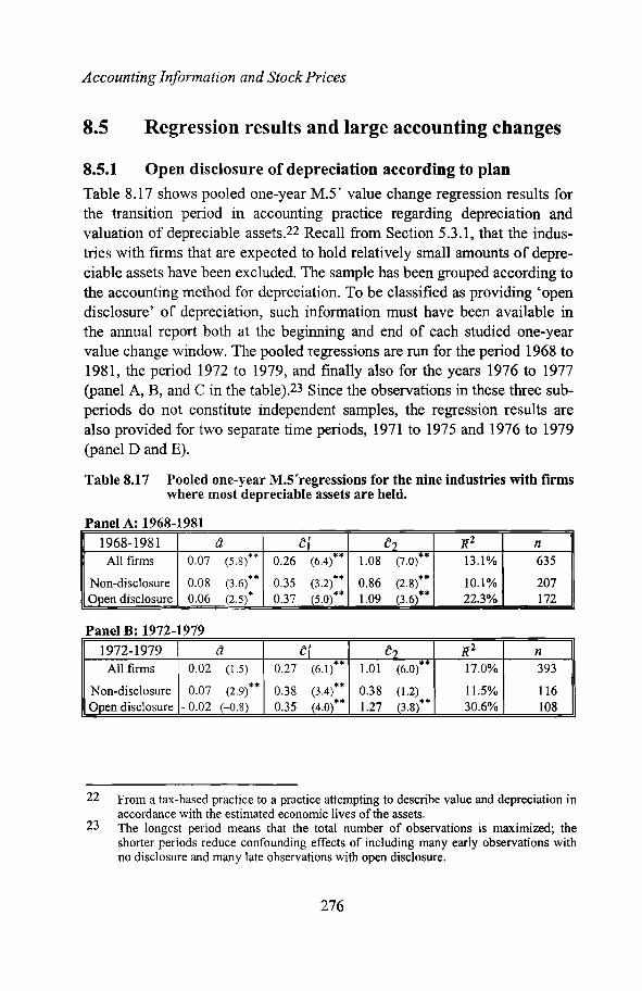
Accounting Information and Stock Prices
8.5 Regression results and large accounting changes
8.5.1 Open disclosure of depreciation according to planTable 8.17 shows pooled one-year M.5' value change regression results forthe transition period in accounting practice regarding depreciation andvaluation of depreciable assets.22 Recall from Section 5.3.1, that the industries with firms that are expected to hold relatively small amounts of depreciable assets have been excluded. The sample has been grouped according tothe accounting method for depreciation. To be classified as providing 'opendisclosure' of depreciation, such information must have been available inthe annual report both at the beginning and end of each studied one-yearvallIe change window. The pooled regressions are run for the period 1968 to1981, the period 1972 to 1979, and finally also for the years 1976 to 1977(panel A, B, and C in the table).23 Since the observations in these three subperiods do not constitute independent samples, the regression results arealso provided for two separate time periods, 1971 to 1975 and 1976 to 1979(panel D and E).
Table 8.17 Pooled one-year M.5'regressions for the nine industries with firmswhere most depreciable assets are held.
Panel A: 1968-19811968-1981 tt ~1 e2 R2 n
All firms 0.07 (5.8)** 0.26 (6.4)** 1.08 (7.0)** 13.1% 635
Non-disclosure 0.08 (3.6)** 0.35 (3.2)** 0.86 (2.8)** 10.1% 207Open disclosure 0.06 (2.5)* 0.37 (5.0)** 1.09 (3.6)** 22.3% 172
Panel B: 1972-19791972-1979 tl ~1 e') R2 n
All firms 0.02 (l.5) 0.27 (6.1)** 1.01 (6.0)** 17.0% 393
Non-disclosure 0.07 (2.9)** 0.38 (3.4)** 0.38 (1.2) 11.5% 116Open disclosure -0.02 (-0.8) 0.35 (4.0)** 1.27 (3.8)** 30.6% 108
22 Fronl a tax-based practice to a practice attempting to describe value and depreciation inaccordance with the estimated economic lives of the assets.
23 The longest period means that the total number of observations is maximized; theshorter periods reduce confounding effects of including many early observations withno disclosure and many late observations with open disclosure.
276

Empirical Results: The Change Approach
Panel C: 1976-1977
1976-1977 d ~f ~2 ]{2 nAll firms -0.08 (-3.4)** 0.29 (4.7)** 1.66 (5.3)** 31.8% 98
Non-disclosure -0.06 (-0.6) 1.03 (1.5) 1.49 (0.8) 6.1% 17Open disclosure -0.13 (-3.6)** 0.51 (4.9)** 0.97 (1.8)* 48.8% 32
Panel D: 1971-1975
1971-1975 d ~f ~2 ]{2 nAll firms 0.13 (6.0)** 0.21 (2.9)** 0.38 (1.6) 4.5% 238
Non-disclosure 0.13 (4.6)** 0.24 (2.0)* 0.54 (1.5) 5.6% 113Open disclosure 0.05 (0.6) 0.49 (1.6) 0.12 (0.1) 4.1% 31
Panel E: 1976-1979
1976-1979 d ~{ e2 ]{2 nAll firms -0.04 (-2.3)* 0.25 (5.3)** 1.77 (8.1)** 32.8% 192
Non-disclosure -0.11 (-1.3) 1.44 (2.3)* 0.55 (0.4) 13.2% 23Open disclosure -0.04 (-1.6) 0.31 (3.9)** 1.68 (5.1)** 44.5% 80
I-statistics in parenthesis, a two-sided test is used for intercepts and a one-sided test for theslope coefficients.* Significant at 0.01 ~ a ~ 0.05** Significant at a ~ 0.01
Analyzing the first three panels, where a more narrow period is successivelystudied, tl1e open disclosure fim1S showed an ]{2 that was twice as high (forthe period 1968 to 1981), and finally eight times as high (for the period1976 to 1977). These results indicate that the open disclosure practiceregarding depreciation and valuation of depreciable assets has indeedprovided a more informative description of the value creation. It is notable,however, that the annual value change during the earlier period (1971 to1975), was very weakly explained irrespective of the chosen accountingprocedure.
277

Accounting Information and Stock Prices
8.5.2 Regression results and acquisition activityThe period 1986-1990 has been identified as unique in terms of acquisitionactivity among listed companies on the Stockholm Stock Exchange. Table8.18 shows annual and pooled one-year M.5' value change regressions withthe sample divided according to acquisition intensity.24 Observations fromindustries with continuous profit recognition have only been included inthese regressions.
Table 8.18 Annual and pooled one-year M.5'value change regressions withthe sample grouped according to acquisition intensity. Observations from industries with continuous profit recognition have beenused.
P I A All fiane : lrm-yearsYEAR t1 ~{ ~2 ]{2 n
1986 0.34 (8.3)** 0.49 (2.4)** 2.43 (2.6)** 13.2% 931987 0.09 (3.3)** 0.20 (0.9) 3.21 (3.8)** 12.8% 991988 0.24 (6.5)** 1.02 (3.6)** 2.19 (3.2)** 21.9% 931989 -0.02 (-0.4) 0.34 (1.1) 1.39 (1.6) 5.0% 951990 -0.21 (-0.2)** 0.69 (4.8)** 1.70 (3.1)** 26.2% 831991 -0.05 (-1.2) 0.61 (4.5)** 2.64 (4.2)** 33.3% 721992 0.00 (0.1) 0.34 (2.1)* 1.47 (2.7)** 19.9% 57
Mean 0.06 0.53 2.15 18.9% 85Pooled 0.07 (4.3)** 0.62 (8.1)** 2.61 (8.9)** 22.5% 592
tt f£ t d bP IBane : lrm-years no a ec e ly any recen acquisl IonsYEAR t1 ~f ~') ]{2 n
1986 0.37 (7.8)** 0.51 (1.9)* 4.09 (3.5)** 19.7% 691987 0.09 (2.8)** 0.24 (1.0) 3.68 (4.2)** 22.7% 621988 0.26 (4.2)** 0.99 (2.1)* 2.41 (2.4)** 17.2% 501989 0.03 (0.2) 0.29 (0.5) 2.01 (1.5) 5.0% 451990 -0.19 (-4.3)** 0.87 (4.0)** 2.40 (2.1)** 29.3% 391991 -0.04 (-0.8) 0.70 (2.9)** 3.34 (3.6)** 38.6% 401992 0.04 (0.8) 0.63 (2.1)* 1.32 (1.3) 16.9% 34
Mean 0.08 0.60 2.75 21.3% 48Pooled 0.09 (4.3)** 0.76 (6.3)** 3.06 (7.1)** 24.5% 339
24 A firm has been classified as having made a recent acquisition during a particular yearif such an acquisition has taken place during the current year or during any of the twopreceding years. See details regarding the identification procedure of acquisitions insection 5.3.2. The illustrated period has been extended to 1992 in order to include thetwo years after the most acquisition-intensive period.
278

Empirical Results: The Change Approach
· ·t·tf~ t d btl tP Ieane : lrm-years a ec e ~y a eas one recen acquisl IonYEAR t1 e{ e2 ](2 n
1986 0.26 (3.2)* 0.51 (1.6) 0.15 (0.1) 3.9% 241987 0.10 (1.7) 0.15 (0.4) 2.33 (1.3) -0.3% 371988 0.23 (4.9)** 1.01 (3.0)** 1.95 (2.1)* 24.2% 431989 -0.06 (-1.0) 0.33 (1.0) 0.51 (0.5) 0.1% 501990 -0.22 (-5.5)** 0.54 (2.7)** 1.52 (2.4)** 21.9% 441991 -0.07 (-1.0) 0.53 (3.1)** 1.86 (2.1)* 24.0% 321992 -0.09 (-1.8) 0.22 (1.4) 0.88 (1.4) 13.8% 23
Mean 0.02 0.47 1.31 12.5% 36Pooled I 0.02 (l.0) 0.49 (5.2)** 2.05 (5.3)** 19.5% 253
t-statistics in parenthesis, a two-sided test is used for intercepts and a one-sided test for theslope coefficients.* Significant at 0.01 S a S 0.05** Significant at a s 0.01
The mean R 2 was 21.5% for the 'no acquisition group', as compared to12.5% for the 'acquisition group'. The slope coefficients (ei and e2), bothshowed higher values, and were more often significant for the firms in the'no acquisition group'. These results imply that change in equity and, especially, change in residual income have a particularly weak explanatory ability of change in market value for companies that have recently been involved in large acquisitions.
It was argued in the previous chapter that the utilized prediction model forexpected next period ROE may be especially weak when substantialchanges, such as large acquisitions, have taken place.25 A small sample offirms for which business magazine forecasts are available, has been used inorder to shed son1e light on this issue. Table 8.19 shows pooled regressionresults for the acquisition intensive period for a small group of companies.The sample has been grouped according to acquisition intensity, and firstrun with the ROE prediction procedure based on historical performance(panel A), and secondly, utilizing earnings forecasts published inAffarsvarlden, the weekly business magazine (panel B).
25 This argument is, of course, also valid for the variable 'change in expected residual income'.
279

Accounting Information and Stock Prices
Table 8.19 Pooled one-year M.5'value change regressions for a small sampleof companies grouped according to acquisition intensity.
Panel A: Change in residual income based on the main ROE predictiondproce ure.
1986-1992 tl e{ e2 ](2 nAll 0.16 (4.0)** 0.16 (0.7) 3.30 (3.8)·· 11.1% 112
No acquisition 0.19 (2.9)** 0.31 (0.7) 5.55 (3.3)** 15.5% 60Acquisitions 0.10 (2.0) 0.08 (0.3) 1.84 (2.0)* 4.0% 52
Panel B: Change in residual income based on earnings forecasts published· Afro .. ld th b · klIn arsvar en, e uSlness wee lY.
1986-1992 tl e{ e2 ](2 nAll 0.10 (3.0)** 0.63 (3.1)** 6.12 (7.0)** 30.6% 112
No acquisition 0.11 (2.2)* 0.79 (2.3)* 8.85 (7.2)** 47.7% 60Acquisitions 0.07 (1.5) 0.35 (1.4) 3.07 (2.6)** 8.6% 52
t-statistics in parenthesis, a two-sided test is used for intercepts and a one-sided test for theslope coefficients.* Significant at 0.01 ~ a ~ 0.05** Significant at a ~ 0.01
Despite the limited sample size, there are some interesting observations tobe made. The observation that it seems more difficult to explain valuechal1ge (with the specified regression model) for firms involved in one orseveral acquisitions remains, irrespective of the earnings predictionapproach used. When basing ROE predictions on historical performance the]{2 was 15.5% for the 'no acquisition group', as compared to 4.0% for the'acquisition group'. Similarly, when the earnings forecasts in Affarsvarldenwere used, ]{2 was 47.7% as compared to 8.6%. Using earnings forecastsfrom the business magazine apparently improve the explanatory powerextensively, both for all observations and for the two subgroups. It isinteresting to note the higher value of the change in residual returnregression coefficients ( e2) when using the earnings forecasts inAffarsvarlden. These estimated slope coefficients indicate strong expectedpermanence of a new performance level. Another interesting observationconcerns the slope coefficient of the change in equity variable. In panel A,where the main mechanical ROE prediction procedure has been used,change in equity added little explanatory power to the change in marketvalue; the t{ coefficients were low and non-significant. However, when thechange in expected residual income was based on Affarvarlden's earnings
280

Empirical Results: The Change Approach
forecasts, the same variable showed higher and more significantcoefficients.26 This implies that a period's change in equity (or a period'searnings) may well be a valid description of the period's value creation thatis associated with the change in the stock price; however, the omission ofusing a variable that captures changes in future expectation--or the use of apoor proxy-may conceal this association. The fact that R 2
, whenAffarsvarlden's earnings forecasts were used, largely exceeded R 2 whenearnings predictions were based on the most recent ROE (30.6% and 11.1%respectively, for all the 112 observations), certainly casts some doubt on thewidely used proxy for unexpected earnings in the market-based accountingliterature (including the proxy used in this study).
8.5.2.1 Goodwill treatment method
Table 8.20 shows pooled one-year M.5' value change regression results,grouped according to the goodwill treatment n1ethod. The firm-yearsaffected by one or several large acquisitions during the acquisition intensiveperiod 1986-1990 plus the following two years have been used. These firmyears have been divided into three groups: i) fa large goodwill write-off thecurrent period', ii) 'a large goodwill write-off any previous period, andiii) "no goodwill write-off'-that is, an ordinary depreciation scheme forcapitalized goodwill has been used. If the goodwill written off reflects a realdrop in value (during the current period) a significant positive ei coefficiel1t is expected. If, however, the write-off is not perceived as representinga real drop in value by the investors, a negative ei coefficient would be expected for the \vrite-off year and normal positive coefficients in thefollowing years.
26 The coefficients were significant at the 1 percent level for all 112 observations, at the 5percent level for the 'no acquisition group', but non-significant for the 'acquisitiongroup'.
281

Accounting Information and Stock Prices
Table 8.20 Pooled one-year M.5'value change regressions with the samplegrouped according to the chosen method and timing of goodwilltreatment. Firm-years from industries with continuous profit recognition being affected by one or several large acquisitions duringthe last and/or the two previous years have been used.
1986-1992 tl e{ e2 ]{2 nAll 0.02 (1.0) 0.49 (5.2)* 2.05 (5.3)• 19.5% 253
No goodwill write-off 0.01 (0.5) 0.57 (5.6)** 1.97 (4.8)*" 23.1% 196Goodwill write-off (t=I) 0.17 (2.3)* -0.06 (-0.1) 3.26 (1.7) 4.7% 21
Goodwill write-off (t=-l, .. ,-6) -0.02 (-0.3) 0.17 (0.6) 1.64 (1.2) 1.7% 36
t-statistics in parenthesis, a two-sided test is used for intercepts and a one-sided test for theslope coefficients.* Significant at 0.01 ~ a ~ 0.05** Significant at a ~ 0.01
According to table 8.20, the firms that have not written off goodwill showed'normal' regression coefficients, whereas the goodwill write-off firmsshowed a non-significant negative ei coefficient for the actual year of thewrite-off, and a non-significant positive ei coefficient for the yearsthereafter. The e2 coefficients were non-significant, and the overallexplanatory power was also very low for the goodwill write-off firms. It hasto be recognized, however, that the sample of firms that wrote off goodwillwas small, making it difficult make any strong inferences.
8.5.2.2 The pooling versus the purchase method
Table 8.21 S110WS annual and pooled regression results for 1970 to 1976,with the sample grouped according to chosen method of consolidation.Observations from industries with continuous profit recognition have beenused.
282

Empirical Results: The Change Approach
Table 8.21 Annual and pooled one-year M.5' value change regressions withthe sample divided according to group consolidation method.
rd fth d d~P rP IAane : 00102 me 0 use or conso I a Ion.a ef e2 ]{2 n
1970 -0.02 (-0.4) 0.15 (0.7) 0.89 (0.7) -2.9% 171971 0.44 (4.3)** -0.05 (-0.1) 3.58 (2.3)* 18.5% 161972 0.14 (3.8)** -0.47 (-1.9) 3.01 (2.6)** 24.1% 231973 0.07 (0.9) 0.09 (0.3) 1.61 (1.9)* 11.1% 201974 0.00 (0.1) -0.08 (-0.5) 0.17 (0.2) -12.8% 161975 0.19 (2.0) 0.83 (3.1)** 1.29 (1.7) 39.8% 141976 0.03 (0.4) 0.45 (1.2) 1.48 (1.7) 20.8% 11
Mean 0.12 0.13 1.72 14.1% 17Pooled 0.14 (4.6)** 0.09 (0.8) 0.46 (1.1) 0.1% 117
Panel B: Purchase method used for consolidation.a ei e2 ]{2 n
1970 -0.10 (-1.4) -0.43 (-0.9) 1.15 (1.4) 2.1% 111971 0.24 (2.2) -0.09 (-0.4) 0.75 (0.4) -17.4% 121972 0.07 (0.9) -0.24 (-0.7) 1.99 (1.1) -4.3% 151973 0.01 (0.1) 0.09 (0.4) 3.14 (4.0)** 52.8% 191974 0.12 (l.5) -0.44 (-1.5) 1.31 (2.0)* 13.3% 211975 0.05 (0.5) 0.72 (2.7)** -1.08 (-1.2) 20.6% 211976 -0.07 (-1.8) 0.17 (1.7)* 1.09 (2.3)* 18.6% 30Mean 0.05 -0.03 1.19 12.2% 18Pooled 0.06 (2.1)* 0.12 (1.3) 0.63 (2.0)* 3.2% 129
t-statistics in parenthesis, a two-sided test is used for intercepts and a one-sided test for theslope coefficients.* Significant at 0.01 ::::; a ~ 0.05** Significant at a ::::; 0.01
Apparently, very weak and unstable regression results have been obtained,irrespectively of the chosen group consolidation method; there is thus noclear difference related to t11e consolidation method to be observed.
8.5.3 Accounting for associated companiesA gradual transition from the cost method to the equity method when accounting for associated companies took place during the 1980s for firmslisted on the Stockholm Stock Exchange. As previously noted, the amountof data available relating to the associated company issue is very limited.No regression results are therefore reported.
283

9 SUMMARY AND CONCLUDING
REMARKS
9.1 Research problem and research designAn important starting point of this study has been the idea that value andvalue creation of a company can be captured from three related, but conceptually different, perspectives. The theoretical construct, economic value,is based on present value calculations of future expected cash flows. Valueaccording to the traditional cost-based accounting measurement procedure isbased on actual transactions, hence actual cash outlays used to gain accessto resources constitute the base for accounting value. The market value of ashare observed on the stock market is based on trade between investors.Value and value creation as manifested in market prices and as described inpublished accounting reports can easily be observed, while economic valuecannot. Assuming that investors use accounting information to evaluate thefinancial status of a firm and to form (or revise) expectations of its futureperformance, a link can be expected between accounting and market values.Given that the valuation approaches used by investors are reasonably consistent with economic valuation theory, a conceptual link can be establishedbetween accounting values and market values based on economic valuationtheory.
The purpose of this study has been to empirically investigate the presence ofsuch a link for Swedish companies. Previous research, using data from othercountries, has-in general--documented inconsistent results and widelyfluctuating regression parameters, when evaluating such associations. It hasbeen argued in this study that stable intertemporal regression paran1eters canhardly be expected. A fundamental difference is generated by market valuesbeing forward-looking (driven by expectations of future performance) andaccounting value being historically oriented (value calculated as a result ofspecific measurenlent procedures that follows conventions and rules).Events that change the expectations of the future performance of a firm may

Summary and Concluding Remarks
affect the stock price instantaneously, whereas the financial consequencesmay not be reflected in the accounting descriptions until several periodslater. This fundamental difference implies that stable regression coefficientscannot generally be expected. Changes in the economic climate and changesin accounting principles can exaggerate such fluctuations. Moreover, the useof differently composed samples of firms is also considered a likely sourceof cross-sectional and intertemporal instability in regression parameters.Thus an important purpose of this study has been to investigate differencesin the association between accounting numbers and stock prices for differentfirm characteristics, changes in the economic climate, and a few majorchanges in accounting practice.
In order to investigate the association in question, it was deemed in1portantto first outline a valuation model that ties accounting value concepts to economic value. Such a valuation model was developed and discussed in Chapter 2. The chosen n10del is based on viewing the value of shareholders'equity as the discounted sum of expected future dividends. The particularvaluation structure utilized, where dividends are substituted with accountingconcepts--essentially earnings and book value of shareholders' equity-canbe traced back to Preinreich (1938).1
Before deriving a valuation model, suitable for large scale empirical testing,two requirements were established. First, return on equity (ROE) should beincluded as a central accounting performance indicator, and second, a variable that captures the consequences of a conservative accounting regin1eshould be incorporated into the valuation equation.
In order to reduce a fairly general valuation expression to a model driven bya few key factors, several rather strong assumptions have been required.First, the basic assumptions are: a flat term structure of the future requiredrate of return, casl1 flows-net dividends--occurring at the end of eachperiod and an accounting language complying with the clean surplusrelation of accounting. Second, the firm's expected growth rate (g) is knownand constant, which in tum implies a residual dividend policy. Third, from
This valuation approach has subsequently been further developed and refined. Theframework used in this study is particularly inspired by the work of Ohlson (1989a,1989b and 1995), Brief and Lawson (1992) and Skogsvik (1993).
285

Accounting Information and Stock Prices
some future horizon point in time (t+1) and onwards the firm is expected togenerate 'normal' profitability. Fourth, the future expected return on equityfollows a mean reversion process (captured by the fading factor 2) fronl thelevel of return on equity expected for the next period. Fifth, an expectedlevel of a relative accounting measurement bias can be assessed. Sixth, therelative accounting measurement bias is assumed to be permanent fromtoday and onwards (thus the bias is denoted PMB).
With this set of assumptions, value (V) at time t has been modeled as follows:2
[2:32](
GoA)TE ROE(b) r 1- --
V =B(b) 0(1 PMB) B(b). (( 1+1)- -r). l+rt t + + t l+r l_(GoA)
1+r
The value of owners' equity is hence described as the sum of two terms: i)the level of current accounting equity adjusted for any measurement bias ofthe accounting regime, and ii) the present value of all abnormal profits thatthe firm is expected to generate from time t to a date T periods ahead. Thelatter element has in tum been formulated as a multiple of three factors: i)the level of current accounting equity, ii) the next period's expected abnormal return (discounted one period), and iii) a factor that depends on a combination of the future expected growth, the development pattern and persistence of abnormal performance, and the discount rate. The hurdle rate usedto calculate abnormal profits has been adjusted to incorporate the annualmeasurement bias, y.
Based on this valuation equation, two level regression models and threevalue change regression models were specified. M.2 is the most completelevel specification utilized in this study:
M.2 ~~,t -1 = a +A ·Et [RRj ,t+1] + Pz ·PMBj + &J,tj,t
2 A list of all symbols and abbreviations are provided at the end of this booko
286

Summary and Concluding Remarks
In specification M.2, the market-to-book value premium is explained by theexpected next period residual return (based on expected ROE) and the PMB.The regression coefficients can easily be given economic interpretations.The sin1plicity of the model is an advantage, but also its main weakness. Allfirms cannot be expected to have the same constant growth potential, to beequally capable of maintaining a competitive advantage or recuperatingfrom the consequences of a poor investment decision, nor to hold such abalanced portfolio of assets that a permanent relative measurement bias canrealistically be expected. An obvious consequence of a lack of stability inthese factors over time and between firms, is that the regression parametersshould be expected to vary and that an explanatory power of less than 100%is to be expected. The constant PMB assumption can be expected to be particularly invalid for firms whose key asset base has an unbalanced agestructure. This situation is most likely to occur for firms that make largediscrete investments in assets with long economic lives. The investment in anew power plant by an electric utility firm, or the investment in a new papermill by a paper and pulp firm, constitute typical examples. Firms growingby making large acquisitions and accounting for these acquisitions using thepurchase method constitutes another example.
Creating tl1fee subgroups based on a priori expectations of the level of thegrowth persistence factor (GPF) and grouping firms according to industrymembership are two ways in which an attempt has been made to add controlfor the problen1s indicated above. It was thus argued that the regressioncoefficients should be expected to be a = 0.0,3.0 <PI < 8.0, and /32 = 1.0for a 'normal' sample of firms.
M.5' is the most complete value change specification that has been utilizedin the study: 3
Pj,t+k-Pj,l , (b j,t+k-bj,t)·(l+PMBj )=a+ct • +
M.5' Pi,t Pi,t
[Et+k (RTj,t+k+l)- Et(RTj,t+I)]+C2 • + '&j,t+k
Pi,t
3 See the list of symbols and abbreviations at the end of this book.
287

Accounting Information and Stock Prices
According to M.5' the change in the stock price (P) between two points intime is explained by the change in book value of equity per share (b), theestimated PMB, and the change in expected residual income (Rl). Thechange in equity is viewed as a measure of the value created (and retained),while the change in expected residual income is an indicator of changes inthe expected profitability of the firm. These interpretations are somewhatdifferent than what has used to be the common practice in the market-basedaccounting researcll literature. For example, in Easton and Harris (1991)earnings levels and earnings changes are viewed as competitive explanatoryvariables of return. In the 'good news' versus 'bad news' setting followingBall and Brown (1968), earnings changes have often been interpreted as asignal (surprise) of a new performance level. However, in the long windowvalue change regressions of Easton, Harris and Ohlson (1992) and Ohlsonand Penman (1992), aggregated earnings have been viewed as a measure ofvalue creation. M.5' thus combines the signaling perspective of Ball andBrown and the measurement perspective of Easton, Harris and Ohlson(1992) and Ohlson and Penman (1992).
Provided that good estimates of the firm-specific residual income are available and that the assumptions of constant GPF and PMB are reasonablyvalid, the following regression coefficients are to be expected: t1 isexpected to be zero, e; is expected to equal one, and e2 is an estimate of thegrowth persistence factor (and should thus be expected to be between 3 to 8for a 'normal' sample).
An important parameter in both the level and the change model specifications of this study, is the expected level of next period ROE. Given previousresearch results regarding earnings and return predictions, and inspired by astudy of Freeman and Tse (1992), a non-linear mean-reversion predictionfunction was chosen. Regression results (presented in Section 6.1.2) com~
paring ROEj,t to ROEj,t+1 supported the hypothesis of one-period persistence in ROE. Notably, a small mean reversion tendency in ROE for nonextreme levels and a larger mean reversion tendency for extreme levels wasobserved.
A rather large effort has been made in order to estimate the extent to whichthe traditional historical cost-based accounting convention tends to under-
288

Summary and Concluding Remarks
state the 'true value' of shareholder's equity. In the conceptual descriptionsin Chapter 3, it was shown that this tendency is different for different typesof tangible and intangible assets, as well as for different types of liabilities.It was further argued that since companies engaged in different businessactivities, hold different combinations of assets and often finance them differently, one should expect different degrees of accounting measurementbiases for different types of businesses. In Chapter 5, a rather crude estimation of permanent measurement biases (PMBs) was performed. These estimations relied on, for example, median indicators of asset type intensity, theeconomic life of the asset type, the equity-to-asset ratio, and the inflationrate. The estin1ation procedure generated a significant spread between, atone end, the pharmaceutical industry with an estimated PMB of 1.74, and atthe other end, the engineering, other production and conglomerate andmixed investment companies with an estimated PMB of about 0.30.
It was argued in Section 3.1.2 that the GPF of a firm could be expected tomainly be a function of the firm's growth potential and the degree of industry competitiveness. It was consequently argued that a high GPF firmshould be characterized by high growth and stable future positive residualreturn, and that a low GPF could be expected for loss firms (negative ROE)and firms with extremely high current ROE. Operationalizations of theseideas were presented in Section 5.1.3.
Published earnings or return on equity are often used as indicators of thefinancial performance of a firm. In this study, return on equity is given suchan interpretation. However, it was argued in Section 3.1.3 that the validityof published earnings (or ROE) as an indicator of a performance level forfuture periods, can be expected to be quite poor for certain types of businessactivities. This short-term ROE validity problem was argued to stem fromthe fact that'the realization principle, combined with certain business characteristics, makes the recognition of profits particularly non-continuous andthe timing particularly open to management discretion in some industries. InSection 5.1.4 the sample of firms was divided into two groups based onindustry classifications to test whether these assertions were valid.
Two aspects of a changing economic climate were considered in thisstudy-the level and the pattern of the inflation rate and the observablefluctuations in the business cycle.
289

Accounting Information and Stock Prices
The diversity and change in the accounting measurement and disclosurepractice between firms and over time, were discussed in Section 3.3.1. Itwas argued that these phenomena obviously add complexity to the empiricalevaluation of the association between accounting information and stockprices. However, it felt unrealistically ambitious to attempt to grasp tIleeffects of all the accounting changes. Thus the ambition stopped at attempting to test/evaluate the effect of a few selected accounting changes change to open disclosure of value and depreciation according to plan,group consolidation method and accounting for goodwill, and the accounting method for associated companies.
9.2 Empirical resultsIn Chapter 4, a sample of Swedish fimls was presented. Data were collectedfor the period 1966 to 1993. Companies were excluded from the sample ifthey i) were not included in the database FINLIS, ii) were not listed formore than four consecutive years, iii) had an accounting period that did notcoincide with the calendar year, and iv) did not provide accounting information according to Swedish GAAP. From the population of all listedSwedish firms, 252 companies were selected. The final sample contains atleast 75% of the total population in terms of firm-years. The absence ofbanks and insurance companies, the loss of relatively many trading andretail companies, and the loss of firms with less than a four-year history onthe stock exchange, constitute the main systematic departures from studyingthe full population of Swedish firms listed on the Stockholm StockExchange during the period 1966 to 1993.
Chapter 7 presented statistical tests based on the specificati()ns M.1 andM.2. A brief summary of the most important results is provided below.
The expected residual return and the permanent measurement bias are bothsignificant explanatory variables for market-to-book values. As return onequity has proven to be an important explanatory variable in previous studies, the importance of the expected residual return variable in this studymight not be surprising. The significance of the industry-specific PMB variable indicates that industries are different in terms of the size of accounting
290

Summary and Concluding Remarks
measurement biases, and that the estimation procedure of the expected PMBproposed in this study captures some of these differences.
When cross-sectional regressions have been repeated annually for the total(heterogeneous) sample of firms, a low explanatory ability, as well as highlyunstable regression coefficients have been observed.
A number of potential sources for the weak and unstable regression resultswere evaluated in Chapter 7. First, it was demonstrated that disclosed ROEis generally a more informative profitability measure for the group of firmscharacterized by profits being recognized continuously. Second, a firm'shistorical stability of ROE was shown to be associated with the estimatedGPF. A higher historical stability was associated with a'higher ]i2 and ahigher GPF coefficient, provided that profit recognition characteristics werecontrolled for. Third, dividing the sample into three ex ante generated GPFgroups indicated that such <;lifferentiation has son1e merit-the estimatedslope coefficients varied in accordance with expectations. Finally, combining these characteristics in an effort to homogenize the sample-selectingfirms with continuous profit recognition, a non-turbulent ROE history, andnon-extreme expected GPF-produced the reasonable mean regressioncoefficients (a =-0.07, PI = 6.04, P2 = 1.09), and a mean ]i2 amounting to44.1%. It was noted that the explanatory power of the regression was particularly poor during the years around 1974 and 1988.
The evidence in Section 7.3.1 provided support for the hypothesis that someof the cross-sectional instability in the regression coefficients has beenrelated to the fluctuations in the business cycle. Clearly, the explanatorypower of the valuation model specification was very low during businesscycle booms, and high during recessions. Alternative reasons for these patterns were discussed, and a hypothesis was advanced implying that stockprices might be 'detached' from fundamentals during boom periods.
In Section 7.3.2 a weakening of the regression results was noted after thenew era of higher and more variable inflation rates which began after the oilcrisis in 1973. For the sub-sample of firms characterized by large holdingsof non-monetary assets with long economic lives, E[RR] was practicallyuseless as an explanatory variable of the market-to-book value premiumduring the period of falling inflation rates (1985-1993). A similar pattern
291

Accounting Information and Stock Prices
was not present for the group of firms holding limited amounts of long-lifeassets.
The results in Section 7.4.1 imply that the more informative, open accounting of value and depreciation of tangible assets that was gradually introduced during the 1970s, has increased the explanatory power of the residualreturn and the PMB variable of the stock price.
Using data from the acquisition intensive period 1986-1990, it was shown inSection 7.4.2 that the usefulness of E[RR] to explain the market-to-bookvalue premium for a group of firms that has recently made large acquisitionsis very limited. After a complementary test on a small sample of firms(utilizing forecasts of earnings published in business magazines), it was suggested that the weak explanatory power is partly related to an inferiority ofthe mechanical prediction approach for firms growing through acquisitions.However, the results are also consistent with tIle hypothesis that acquisitionintensive firms are more complex and difficult to value.
A priori, the capitalization of goodwill was expected to be a more descriptive accounting valuation principle. Nevertheless, the level of ROE appearedto have a very linlited ability in explaining the market-to-book value premium for the average acquiring finn with capitalized goodwill. This result isshown both for the early 1970s, contrasting firms choosing the poolinginstead of the purchase method, and for the period 1986-1992, contrastingfirms writing off goodwill directly against equity versus firms that havechosen to capitalize and amortize goodwill.
The statistical tests based on value change specifications M.3, M.4 and M.5'reported in Chapter 8 generated, in summary, the following results:
In Section 8.1, the change in market value was explained by created andretained value as measured by the accounting convention using regressionspecification M.3. The annual change in book value of equity was firstshown to explain a significant but small part (less than 10%) of the annualchange in the market price. This result was found to be comparable toresults in several previous US studies. By increasing the time interval overwhich value creation was measured, and aggregating the change in bookvalue of equity up to a ten-year period, a monotonous increase from an R2 of
292

Summary and Concluding Remarks
8.7% to 35.4% was shown. A similar pattern has previously been shown forUS data by Ohlson and Penman (1992) and Easton, Harris and Ohlson(1992). Another observation that the studies have in common is that theslope coefficients of the regressions increased as the time interval was prolonged, and exceeded 1.0 for the longer intervals. In this study, this patternhas been interpreted as an indication of a permanent conservative accounting measurement bias.
In Section 8.2 another explanatory variable was added to the regressionmodel, namely change in expected residual income. This variable washypothesized to capture changes in expectations regarding the firm's abilityto create value and it was shown to add significantly to the explanation ofchanges in stock prices. The relative contribution was largest for the twoshorter intervals. For the 5- and 10-year intervals change in book value ofequity became the most important explanatory variable. One conclusion isthus t11at in the short run, changes in the expectations of the future prospectsof a specific firm's ability to deliver abnormal performance, have a verystrong impact on price changes. As the time interval is prolonged, createdand retained value as described by growth in book value of equity becomesan increasingly important explanatory variable.
In Section 8.3, specification M.5' was used as a refinement of M.4. Thechange in book value of equity for each firm was multiplied by (1+PMB)before the regressions were re-run. The study of a heterogeneous sample offirms, combined with expected different accounting consequences for different types of business activities using the prevailiI1g conservative accounting convention, was the rationale behind this specification.4 For thetwo longer intervals, M.5' showed significantly improved explanatorypower. This increased explanatory power was interpreted as supporting thehypothesis that firms are different with respect to their degree of measurement bias, and that the estin1ation procedure of this study in fact capturessome of these differences.
In Section 8.3.1, dividing the sample into two groups according to profitrecognition characteristics, showed that the change in book value of equityl1ad very similar explanatory ability for the two subgroups, whereas the
4 Recall that M.5' was chosen instead of M.5 due to problems of multicollinearity.
293

Accounting Information and Stock Prices
change in residual income variable was more often significant, had a highercoefficient, and added more to the total explanation for the companiescharacterized by a more continuous profit recognition pattern. Thus thevalue relevance and information content of reported ROE appears to bedifferent for different types of business activities. These differences werealso observed when pooled regressions were run separately for differentindustries.
The results in Section 8.4.1 indicate that firms for which the specifiedchange in residual income is a poor proxy for the changed ability to perform(the discrete profit recognition firms), onlission in controlling for changes inthe business cycle causes the largest reduction in explanatory power.
The results in Section 8.5.1 indicate that the transition to an open disclosurepractice, regarding depreciation and valuation of depreciable assets, hasgiven more infornlative descriptions of value creation and of value creationability.
The results in Section 8.5.2 imply that change in equity, and especiallychange in residual income, have a particularly weak explanatory ability forcompanies that have recently been involved in large acquisitions. Thisobservation was shown not to be sensitive to the chosen prediction approachfor next period's ROE.
The value change research design failed to produce any conclusive resultsregarding the goodwill treatment issue and the consolidation issue.
294

Summary and Concluding Remarks
9.3 The validity of the applied research designThe association between certain selected accounting numbers and stockprices has been studied for a sample of Swedish firms over a period ofalnlost 30 years. A number of observations and conclusions regarding theassociation have been advanced. The validity of these conclusions is obviously an important issue, and will be discussed using the taxononly of Cookand Campbell (1979). The structure of the discussion is inspired by Ball andFoster (1982), who, in a methodological review article, illustratively usedthis taxonomy to discuss empirical accounting research problems. Cook andCampbell (1979) distinguished between i) internal validity, ii) constructvalidity, iii) statistical conclusion validity, and iv) external validity.
Internal validity"Internal validity refers to the approximate validity with which we infer thata relationship between the variables is causal or that the absence ofa relationship implies the absence of cause."5 A basic result in this study is thatvalue and value creation as manifested in the stock price can (partly) beexplained with value concepts from the accounting convention (book valueof equity, earnings and return on equity). The internal validity of this conclusion is backed up by the formal modeled link between accounting variables and economic values. The theoretical fundament for a causal linkemanates from the assumption that good financial performance generateslong-run capacity to pay dividends, which in tum is assumed to be appreciated by investors. To dispute this link, one fundamentally has to dispute theidea of capital value being a function of discounted future dividends. However, it is important to note that accounting descriptions per se are not regarded as the cause of stock prices (or movements). The underlying cause isthe business activities that accounting attempts to describe. The issue is thuswhether accounting is successful in providing useful descriptions of tIle realphenomena. From another perspective, if a significant association betweenaccounting performance and stock prices had not been documented, onecould have argued that the valuation specification (including the predictionofnext period's ROE) is too simplistic to capture the details of the link, thatthe accounting procedure generates completely uninformative descriptionsof value and value creation, and/or that the market is irrational (that is, it
5 Cook and Campbell (1979, p. 37), quotation from Ball and Foster (1982, p. 180).
295

Accounting Information and Stock Prices
does not use accounting information in a rational way). This line of argumentation implies that the regression tests performed in this study are inreality simultaneous tests of several issues. The fact that the observed associations are far from being perfect, points at a general difficulty in assessingthe relative 'noise contribution' from each potential type of problem. Thisobservation is important to keep in mind as some particular issues have beenevaluated relying largely on the relative strength of the measured association.
A number of propositions of causal relationships have been advocated andsubsequently evaluated in this report:» Involvement in certain types of business activities makes it difficult for
traditional cost-based accounting to describe value and short-term valuecreation. The regression results presented (both level and change) support this proposition. However, it cannot be completely ruled out thatthese results can be partly driven by, for example, the chosen valuationspecification being more suitable for a certain type ofbusiness activities.
» High and varying inflation rate levels cause particular interpretationproblems ofshort-term accounting performance for some types offirms.The level regression results support this proposition, whereas the changespecification provides rather inconclusive indications.
» More informative accounting procedures should cause better mappingbetween accounting descriptions and stock prices. The empirical evaluation of the transition to an open disclosure practice, regarding depreciation and valuation of depreciable assets, has provided considerable evidence of such a relationship.
» Acquisition intensity causes particular interpretation problems ofshortterm accounting performance. The regression results presented (bothlevel and change) support this proposition.
The nUlTlber of factors that may influence the stock price of a firm at a particular point in time, however, is enormous and the possibility to fully control for all factors (except for the particular one under study) in a real settingis rather limited. Ball and Foster (1982, p.180) discuss two different threatsto internal validity: "Ambiguity about the direction ofcausal inference" and"Selection ".
296

Summary and Concluding Remarks
Several studies have documented that market prices lead accounting earnings (or that market-to-book values can predict future accounting retum).6This observation, however, cannot be interpreted as a causal relationship. Ahigh stock price does not cause good performance. The observation ismerely a reflection of the fact that market prices are future oriented andaccounting measurements tend to lag behind, documenting realized transactions.
USelection" occurs when "an effect may be due to the difference between thekinds ofpeople in one experimental group as opposed to another".7 In thecreation of sample designs, several steps have been taken in this study tominimize the chance of presence of systematic confounding effects (forexample, by homogenizing the sample). In the study of accounting practicetransition, such systematic differences still appear to have been present. Forall the accounting issues that have been studied, a striking and consistentpattern can be observed regarding the gradual transition to a new accountingpractice. The early adapting firms have consistently had a higher mean estimated PMB.8 The early adapters of the new accounting procedures havethus apparently been over-represented by firms in industries which havebeen classified as having a large permanent measurement bias. A commondenominator for the companies with business characteristics that generatelarge accounting measurement biases, is that their business activities areparticularly difficult to describe within the traditional accounting language.In Skogsvik (1993c) it is argued that managers of companies that perceivetheir shares to be undervalued have the strongest incentive to adopt morevalue-relevant accounting practices. A reasonable analogy suggests thatcompanies whose businesses are difficult to capture with accounting descriptions will have incentives to lead the accounting development.
A consequence of this line of reasoning is that if the early adopters of newaccounting procedures tend to be firms with more complex business activi-
6
78
See, for example, Beaver, Lambert and Morse (1980), Warfield and Wild (1992) andPenman (1994).Cook and Campbell (1979, p.37), quotation from Ball and Foster (1982, p. 180).See Section 7.4.1 regarding the change to open disclosure of depreciation according toplan, Section 7.4.2.1 regarding the early goodwill write-off firms, Section 7.4.4.2 regarding the switch to the purchase method firms for group consolidation, and Section7.4.3 regarding the switch to the equity method when accounting for associated companies.
297

Accounting Information and Stock Prices
ties, an observed relative change in explanatory power can be systematicallybiased. Such issues may have particularly influenced the results related tocapitalized goodwill.
Construct validityHConstruct validity refers to the possibility that the operations which aremeant to represent a particular cause or effect construct can be construedin terms ofmore than one construct... What one investigator interprets as acausal relationship between the theoretical constructs labeled A and B,another investigator might interpret as a causal relationship between constructs A and Y or between X and B or even between X and y"9 Ball andFoster (1982, p.182) add: HWhen making inferences from empiricalresearch, the tightness of the linkage between theoretical constructs andtheir operational proxies is a major concern. "
An illustrative example of a variable that is chosen to be proxy for a largenumber of theoretical constructs in the accounting research literature is firmsize; it has been used in different studies to be a proxy for factors such ascompetitive advantage, information production costs, political costs, andrisk. 10
The choice of empirical proxies to represent the theoretical constructs ofthis study has been ratl1er straightforward. Change in book value of equitydescribes (retained) value creation. Expected ability of a firm to perform isbased on current accounting performance (ROE). This is thus a direct test ofthe strength of the current accounting perfom1ance signal as a performanceindicator. However, it is obvious that this 'mechanic' prediction procedurecan neither capture large shifts regarding the general business climate, norparticular circumstances affecting a certain firm. An alternative proxy forexpected performance was utilized on a limited sub-sample (business magazine forecasts of next period's ROE.) This proxy was shown to be moredistinct, but appears to convey similar overall results. Nevertheless, thequalitative difference between the two approaches are not insignificant.
9 Cook and Campbell (1979, p.59), quotation from Ball and Foster (1982, p. 182).10 See discussion in Ball and Foster (1982, p. 190).
298

Summary and Concluding Remarks
Several measurement issues concerning earnings, equity, ROE and cost ofcapital (and its components) were discussed in Chapter 4. A number of precautions and tests were utilized to check that the chosen definitions did notintroduce systematic errors. Change in expected ability to create value hasbeen operationalized as the change in expected residual income. This proxymay be viewed as a continuous version of Ball and Brown's (1968) 'goodnews' versus 'bad news' variable, but furthermore also incorporating thecost and size of equity capital as inputs in the indicator. The final basic construct, the PMB, is obviously measured with error. It has been crudely estimated as constant within industries and over time. This theoretical constructis meant to capture the relative degree of conservativeness in the accountingdescriptions. As this conservativeness is expected to be systematically different for different types of business activities, it is obvious that the size ofthe PMB may also be a proxy for other aspects.
In this study, additional theoretical constructs that in some way have beenconstructed proxies for include: the ex ante classification of data into threeGPF groups based on historical performance and growth rates; the classification of industries into two groups--discrete and continuous profit recognition-based on an idea of difference in the expected validity of historicalaccounting ROE as an indicator of performance; the use of the long-termhistorical change in the Swedish consumer price index as a basis for theidentification of four distinct sub-periods; a particular index of the utilization of resources in the Swedish industrial sector used to capture the phasesof the Swedish business cycle, and finally, three different examples of accounting change. None of these constructs are likely to be perfect. However,I believe that they all capture rather well what they are meant to capture.
Statistical conclusion validityHIn evaluating any experiment, three decisions about covariation have to bemade with the sample data at hand: (1) Is the study sensitive enough topermit reasonable statements ofcovariation? (2) If it is sensitive enough, isthere any reasonable evidence from which to infer that the presumed causeand effect covary? And (3) Ifthere is such evidence, how strongly do the twovariables covary? "11 Ball and Foster (1982, p. 186) add: HA key factor in
11 Cook and Campbell (1979, p. 39), quotation from Ball and Foster (1982, p. 186).
299

Accounting Information and Stock Prices
accounting research is the number ofobservations available to make inferences about covariation. "
The study of Swedish data is quite limiting in a sample-size sense. Thenumber of annual observations in this study varies between 39 and 169;however, the full sample consists of more than 2,000 firol-years. Naturally,when attempting to control for different factors (e.g. profit recognition characteristics and GPF-group) the sample sizes are further reduced. This meansthat it is practically impossible to control for all potential factors simultaneously. Thus, most tests have been performed attempting to control for one ora few factors at a time. Given this restriction, the sample sizes generallyappear to have been large enough to generate fairly robust results. The signand significance of regression coefficients are shown to be fairly consistentand generally 'behave' in line with a priori expectations. The sample sizeproblem is most severe in the study of different accounting procedurechanges. These changes naturally only take place over a few years, and donot necessarily involve all firms. Concerning the change to an open disclosure practice regarding depreciation and valuation of depreciable assets, thedegree of improvement of information quality appears to be so large that itstill can be captured with the utilized research design. Finally, even thoughproblems with multicollinearity and heteroscedasticity do not appear to havebeen severe in this study, some general precaution is always recommendedwhen interpreting tIle results from a small sanlple study relying on an ordinary least square regression technique.
External validity.UExternal validity refers to the approximate validity with which we can inferthat the presumed causal relationship can be generalized to and acrossalternate measures of the cause and effect and across different types ofpersons, settings, and times. "12 Ball and Foster (1982, p. 188) add: UExternalvalidity issues do not arise in projects whose sole object is to describe aparticular data base. ... Projects which deal with populations also do notraise external validity problems. ... Typically, however, authors (or readers)do seek to generalize the findings of a study beyond the sample offirmsexamined or the time period covered. "
12 Cook and Campbell (1979, p. 37), quotation from Ball and Foster (1982, p. 188).
300

Summary and Concluding Remarks
The fact that this study deals almost with the whole population of Swedishlisted firms during the period 1966-1993 implies that the external validityproblem is not a key issue. However, it does not seem unreasonable to attenlpt to generalize the results to other time periods, and to attempt to drawparallels with other countries. 13 A general observation from this study isthat the regression results (the size of coefficients and the strength of theassociation) are sensitive to the composition of the sample (in terms of firmcharacteristics), the economic climate, the relative frequency ofacquisitions, and the quality of accounting information. This observationconstitutes a strong general warning against making 'unreflected' comparisons over time and between samples.
13 "A very healthy trend in the literature is the existence ofresearchers in different countries examining similar questions." Ball and Foster (1982, p. 187).
301

Accounting Information and Stock Prices
9.4 Concluding remarksThe often documented weak ability of accounting earnings to explain thelevel of stock prices and changes in stock prices for short periods can beattributed to:
i) the limited ability in general of traditional cost-based accounting to describe value creation for shorter periods, an ability being disparate fordifferent types of business activities, which in tum appears to be magnified by, for example, 'troublesome' inflationary periods;
ii) the sample studied often being heterogeneous in terms of industrialdiversity, firms with different growth potential and competitive conditions, acquisition activity differences, and accounting procedures employed;
iii) the common use of a rather simple operationalization of future performance expectations.
The often documented intertemporal instability in regression coefficientshas further been shown to partly stem from the fluctuations in the businesscycle.
Prolonging the perspective, change in book value of shareholders' equitycan describe an increasing amount of the value creation as expressed bychanges in stock prices. In other words, value relevant events appear sooneror later to be incorporated into the accounting descriptions. It has beenargued that the observation that one unit of change in equity seems to beassociated with more than one unit of change in stock price, largely stemsfrom the general use of a prudent cost-based accounting convention.
It has, furthermore, been shown that the disclosed level of earnings of a firmis associated with changes in the stock price beyond what is merelyreflected in the growth in shareholders' equity resulting from the currentearnings level. Earnings thus appear to provide it1formation regarding bothvalue creation of the period and the firm's ability to generate future value.
302

Summary and Concluding Remarks
The study of a number of sub-samples of firms possessing different firmcharacteristics, changes in the economic climate and changes in accountingprocedures has further generated a number of insights:
i) large amounts of assets with long economic lives appear to nlake shortterm historical cost-based accounting descriptions particularly poor asindicators of value creation. Furthermore, high and varying inflationrates appear to magnify these problems;
ii) the accounting change leading to open disclosure of value and depreciation according to plan of tangible assets, has evidently led to more informative descriptions. However, it is not clear whether the market can(does) take advantage of information on acquired and capitalized goodwill.
A discussion of sonle additional implications of this study's results from theperspective of three presumably interested parties-investors, providers ofaccounting information and standard setting bodies, and researchcolleagues-will conclude this report.
Implications for investorsAccounting as a language for evaluation ofdifferent scenariosLong-term stock market value changes have been shown to correlate wellwith long-term growth in book value of equity. If long-term growth in bookvalue of equity can be projected, an important aspect of the future stockprice of a company can thus be predicted. This implies that the generation oflong-term projections in terms of future income statements and balancesheets appears to be a sensible endeavor.
Terminal value calculationsWhat market-to-book value of equity can be expected for a firm in a steadystate generating a perpetual 'normal performance' from tinle t+T and beyond? If projections of future income statements and balance sheets areperformed utilizing traditional conservative accounting concepts, the idea ofdifferential effects in terms of an accounting measurement bias for differentbusiness activities could be utilized. The estimated PMBs in this study appear to have empirical validity, which implies that the estimation procedurefor evaluating an expected PMB outlined in this study could be useful whenestimating the terminal value.
303

Accounting Information and Stock Prices
Terminal valuej,t+T= Equity j,t+T ·(1+PMBj )
This approach can be used as a complen1ent or an alternative to the commonly used perpetual growth formula.
Fundamental analysis and the business cycleStock prices appear to have been detached from fundamental accountingvariables in and around the periods of economic boom. This pattern hasconsequently been present for the whole period studied, 1967-1993. Thismay n1ean that some fundamental variable is missing in common valuationspecifications or that a systematic market inefficiency exists that can possibly be exploited.
A suggested alternative to PIE ratio comparisonThe comparison of PIE ratios for different firn1s in an endeavor to find overor under-priced shares is commonplace in the investment community. Arather simple, but potentially richer alternative can be specified given thevaluation approach presented in Chapter 2 of this study. First, calculate theimplicit growth persistence factor (GPF) given a company's stock price,current book value of equity, expected ROE for the next period, cost of equity capital, and the expected PMB. In other words, what GPF is necessaryto justify the current stock price? Secondly, compare the implicit GPF levelfor different firms. How realistic the GPF values are can be evaluated interms of differences in, for example, expected growth opportunities andheights of barriers to entry. Tables such as 2.3a-e, presented in Chapter 2,can be used to evaluate required combinations of growth and sustainabilityof abnormal performance to justify a particular price level.
Implications for providers of accounting information andstandard setting bodiesThe research design of this study can at best provide evidence concerning'how the world works'. Walker (1997) notes that one cannot deliver directpolicy advice from market-based accounting research:
H ••• because you can never derive a normative proposition frompositive observations alone. Someone needs to specify what the
304

Summary and Concluding Remarks
objectives are, then MBAR may be able to help advising how toachieve those objectives. "
Walker (1997, p. 344)
The result of this study that indicates an informative advantage for the firmsthat switched to an open disclosure practice of value and depreciation oftangible assets,14 appears to be an instructive example of 'improved accounting principles', given that an objective of 'good accounting' is to provide information that is useful and relevant for investors.
To apply the valuation model utilized in this study, a difficult but necessarytask is the calculation of a measurement bias. The measurement bias is theresult of an application of traditional conservative accounting principles. Ithas been argued that the main sources of an understatement of value according to the Swedish (and probably most western) accounting conventionsare the valuation of long-lived tangible assets at historical cost and the tendency to treat expenditures that create intangible assets, such as R&D,brandname development and personnel training, as expenses. There areprobably good reasons for the existence of such prudent accounting conventions, given the uncertainty regarding future benefits associated with theseitems. Investors that wish to make their own judgment of the PMB for aparticular firm could, however, be assisted by more information regardingannual R&D, marketing and personnel training expenditures. Informationregarding the age structure of the tangible asset base as well as current costor market values of important tangible assets could also prove helpful.While it is easy to always ask for more information, issues such as information production costs and consequences of information overload should, ofcourse, not be neglected.
Implications for researchers and suggested future researchIt was argued early in this study that the bottom-line measure of earningsdisclosed in an income statement can be viewed from two perspectives-asa measure of the firm's value creation during a period and as an indication(or signal) of the firm's ability to create value. These two views constitutedthe base for the value change regression specifications M.4 and M.5, where
14 The informative advantage appears to have led to a better statistical map between thestock price (and stock price changes) and fundamental accounting variables such asROE and book value of equity.
305
II Runsten

Accounting Information and Stock Prices
value change has been explained by both change in book value of equity(value creation) and change in expected residual return (change in expectedability to create value). This view is conceptually different from the'competitive view' of the role of 'earning levels' versus 'earnings changes'as explanatory variables of return found in many published MBAR articles.Studying raw return, it appears important to include both variables in orderto achieve economically sensible regression coefficients (unless the variation in the other variable somehow is controlled for). It has been suggestedthat the regression coefficients that should be expected for these two variables are 1.0 for the value creation variable, and around 3 to 8 (for normalGPF firms) for the change in value creation ability variable.
Historical short-term accounting performance appears to be a particularlypoor starting point for predictions of future performance for business activities characterized by non-continuous profit recognition. Expected ROE andchange in (expected) residual income have generally had a lower slope coefficient and have less often been significant for the firms in the long production cycle industries with revenue recognition at completion (i.e. buildingand construction firms) and for the 'holding-gain-intensive' industries (suchas real estate, shipping and investment companies).
It should be noted that in certain years several of these firms have voluntarily disclosed the market value of their key assets. These voluntary disclosures have not been utilized in this study. It would, however, be interestingto extend this study to also include these reported unrealized holding gainsin the book value of equity and the annual change in the unrealized holdinggains in the earnings measure. The inclusion of these unrealized holdinggains should, of course, reduce the expected level of the PMB and the returnon equity measure could be expected to become more value relevant. Anobvious problem relates to the lack of an accepted standard procedure forthese value calculations and the resulting uncertainty of the estimated unrealized holding gains.
The observation that one unit of retained earnings seems to be associatedwith more than one unit of market value change, as observed in Ohlson andPenman (1992) and Easton, Harris and Ohlson (1992), has been suggested tostem from the existence of an accounting measurement bias. The mean level
306

Summary and Concluding Remarks
of the slope coefficient for the longer time intervals is consistent with theestimated levels ofPMBs.
It has further been observed that the slope coefficient of the change in expected residual return variable increases as the studied time interval is prolonged. For the ten-year interval, the coefficient has generally reached approximately the same levels as the residual return variable showed in thelevel specification (the coefficient being, of course, also an indication of theGPF). These results are in accordance with the conclusions advanced inKothari and Zimmerman (1995), stating that the earnings response coefficients are substantially less downward biased in price models than in returnmodels. This downward bias for the return specification appears to be reduced when the return interval is prolonged. Further, this downward biasmay also explain why the I-year value change specification appears to bemore sensitive to small sample sizes than the levels approach.
The empirical results of this study imply that the common use of heterogeneous samples of firms (both in terms of types of business activities andchosen accounting measurement procedures) can explain parts of the oftenobserved unstable regression coefficients and the commonly low R2 inmarket-based accounting research. Additionally, the fluctuations in thebusiness cycle have been shown to constitute a very important source ofinstability for both regression coefficients and the R2s in the Swedish sample of firms. Thus, the previously suggested warning against making'unreflected' comparisons over time and between samples should be emphasized once again.
It has been suggested that a poor proxy for, for exan1ple, expected next period ROE (or EPS), besides giving po~r statistical fit in general, may alsoconceal the association of another relevant explanatory variable, such as thechange in book value of equity (in value change specifications such as M.4or M.5).l5
Several research questions that have not been explicitly addressed in thisreport have surfaced during the process ofperforming and documenting thisstudy. Obvious extensions include the study of: the potential benefit of util-
15 See discussion in Section 8.5.2.
307
Accounting Information and Stock Prices
izing firm- and time-specific PMBs, the consequences of new accountingissues such as the switch to the percentage of completion method, and thevalue relevance of voluntary disclosures of market values of certain longlife assets. PMBs have been estimated through a procedure where estimatedpartial PMBs have been added to a total PMB. Each partial PMB emanatesessentially from conservative valuation of different types of material andimmaterial assets. It would thus be possible to evaluate the relevance ofeach source of the bias, given that decomposed measures of the PMB areincluded in a regression. A general investigation of the usefulness of thepermanent measurement bias concept in other countries could also beperformed.
The fact that the switch from the cost method to the equity method whenaccounting for associated companies tends to imply a simultaneous increasein both book value of equity and return on equity, constitutes a particularlyinteresting situation which deserves further research attention. To increasethe statistical validity of such a test, this question should preferably be empirically evaluated in a country where more observations can be obtainedthan in the Swedish case.
It would also be interesting to investigate on a broader international scalewhether different phases of the business cycle are associated with similarregression patterns as observed in this study on Swedish data.
In a study of the accuracy and explainability of dividend, free cash flow andabnormal earnings valuation models, Francis, Olsson and Oswald (1997)utilize two principally different approaches to calculate the terminal value: aPIE value approach using expected earnings at time t+T and a Gordonapproach using free cash flow, dividends and abnormal earnings at time t+Tas a starting point in perpetual calculations (with and without growth). Athird approach, consistent with the valuation model suggested in this study(provided that T is set large enough to ensure that it is reasonable to expectthat the firm will only generate normal true performance), would be to calculate the terminal value as expected book value of equity at time t+T times1+PMB given the dividend approach, as expected book value of capitalemployed at time t+Ttimes 1+PMB of capital employed given the free cashflow approach, or as expected book value of equity at time t+T times thePMB given the abnormal earnings valuation approach.
308

Summary and Concluding Remarks
Several studies have documented a so-called PIE effect, where portfolios ofhigh PIE ratio firms have underperformed in comparison to low PIE ratiofirms. A similar evaluation of a trading strategy based on high and low implicit GPFs could constitute an interesting extension.
309

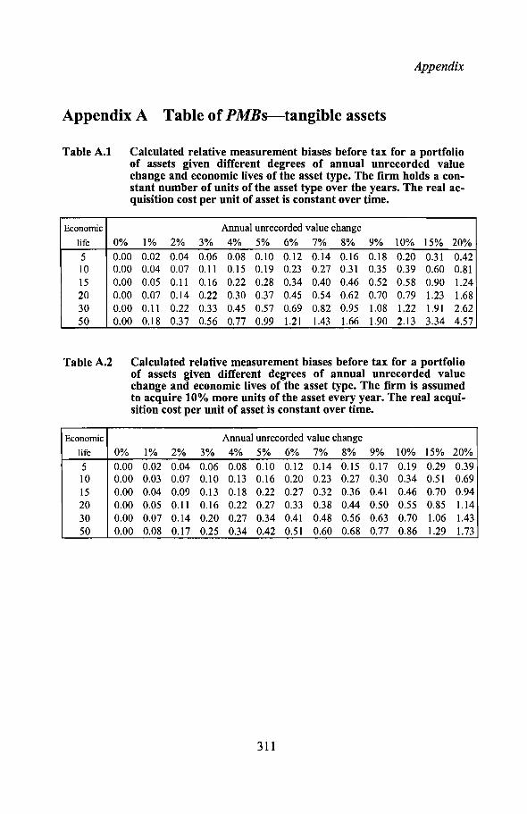
Appendix
Appendix A Table of PMBs-tangible assets
Table A.1 Calculated relative measurement biases before tax for a portfolioof assets given different degrees of annual unrecorded valuechange and economic lives of the asset type. The firm holds a constant number of units of the asset type over the years. The real acquisition cost per unit of asset is constant over time.
Economic Annual unrecorded value change
life 0% 1% 2% 3% 4% 5% 6% 7% 8% 9% 10% 15% 20%
5 0.00 0.02 0.04 0.06 0.08 0.10 0.12 0.14 0.16 0.18 0.20 0.31 0.4210 0.00 0.04 0.07 0.11 0.15 0.19 0.23 0.27 0.31 0.35 0.39 0.60 0.8115 0.00 0.05 0.11 0.16 0.22 0.28 0.34 0.40 0.46 0.52 0.58 0.90 1.2420 0.00 0.07 0.14 0.22 0.30 0.37 0.45 0.54 0.62 0.70 0.79 1.23 1.6830 0.00 0.11 0.22 0.33 0.45 0.57 0.69 0.82 0.95 1.08 1.22 1.91 2.6250 0.00 0.18 0.37 0.56 0.77 0.99 1.21 1.43 1.66 1.90 2.13 3.34 4.57
Table A.2 Calculated relative measurement biases before tax for a portfolioof assets given different degrees of annual unrecorded valuechange and economic lives of the asset type. The firm is assumedto acquire 10% more units of the asset every year. The real acquisition cost per unit of asset is constant over tinle.
Economic Annual unrecorded value change
life 0% 1% 2% 3% 4% 5% 6% 7% 8% 9% 10% 15% 20%
5 0.00 0.02 0.04 0.06 0.08 0.10 0.12 0.14 0.15 0.17 0.19 0.29 0.3910 0.00 0.03 0.07 0.10 0.13 0.16 0.20 0.23 0.27 0.30 0.34 0.51 0.6915 0.00 0.04 0.09 0.13 0.18 0.22 0.27 0.32 0.36 0.41 0.46 0.70 0.9420 0.00 0.05 0.11 0.16 0.22 0.27 0.33 0.38 0.44 0.50 0.55 0.85 1.1430 0.00 0.07 0.14 0.20 0.27 0.34 0.41 0.48 0.56 0.63 0.70 1.06 1.4350 0.00 0.08 0.17 0.25 0.34 0.42 0.51 0.60 0.68 0.77 0.86 1.29 1.73
311

Accounting Information and Stock Prices
Appendix B Table ofPMBs-intangible assets
Table A.3 Calculated relative measurement biases for different degrees ofannual expenditures in an intangible asset and different investment-to-harvest timelags. The reported solidity has been set equalto 50% and the tax rate set at 30°At. The real discount rate andannual growth have been set at 5% and 100/0 respectively.
Time Annual relative expenditure (expenditure/total assets)Lag 0% 1% 2% 3% 4% 5% 6% 7% 8% 9% 10% 15% 20%
0 0.00 0.00 0.00 0.00 0.00 0.00 0.00 0.00 0.00 0.00 0.00 0.00 0.001 0.00 0.01 0.03 0.04 0.06 0.07 0.08 0.10 0.11 0.13 0.14 0.21 0.282 0.00 0.03 0.05 0.08 0.11 0.14 0.16 0.19 0.22 0.25 0.27 0.41 0.553 0.00 0.04 0.08 0.12 0.16 0.20 0.24 0.28 0.32 0.36 0.40 0.60 0.804 0.00 0.05 0.10 0.16 0.21 0.26 0.31 0.37 0.42 0.47 0.52 0.78 1.055 0.00 0.06 0.13 0.19 0.26 0.32 0.38 0.45 0.51 0.58 0.64 0.96 1.286 0.00 0.08 0.15 0.23 0.30 0.38 0.45 0.53 0.60 0.68 0.75 1.13 1.507 0.00 0.09 0.17 0.26 0.34 0.43 0.51 0.60 0.68 0.77 0.86 1.28 1.718 0.00 0.10 0.19 0.29 0.38 0.48 0.57 0.67 0.77 0.86 0.96 1.44 1.919 0.00 0.11 0.21 0.32 0.42 0.53 0.63 0.74 0.84 0.95 1.05 1.58 2.11
10 0.00 0.11 0.23 0.34 0.46 0.57 0.69 0.80 0.92 1.03 1.15 1.72 2.29
Table A.4 As above, but the real discount rate and annual growth have beenset at 100/0 and 0% respectively.
Time Annual relative expenditure (expenditure/total assets)Lag 0% 1% 2% 3% 4% 5% 6% 7% 8% 9% 10% 15% 20%
0 0.00 0.00 0.00 0.00 0.00 0.00 0.00 0.00 0.00 0.00 0.00 0.00 0.001 0.00 0.01 0.03 0.04 0.06 0.07 0.08 0.10 0.11 0.13 0.14 0.21 0.282 0.00 0.03 0.06 0.09 0.12 0.15 0.18 0.21 0.24 0.26 0.29 0.44 0.593 0.00 0.05 0.09 0.14 0.19 0.23 0.28 0.32 0.37 0.42 0.46 0.70 0.934 0.00 0.06 0.13 0.19 0.26 0.32 0.39 0.45 0.52 0.58 0.65 0.97 1.305 0.00 0.09 0.17 0.26 0.34 0.43 0.51 0.60 0.68 0.77 0.85 1.28 1.716 0.00 0.11 0.22 0.32 0.43 0.54 0.65 0.76 0.86 0.97 1.08 1.62 2.167 0.00 0.13 0.27 0.40 0.53 0.66 0.80 0.93 1.06 1.20 1.33 1.99 2.668 0.00 0.16 0.32 0.48 0.64 0.80 0.96 1.12 1.28 1.44 1.60 2.40 3.209 0.00 0.19 0.38 0.57 0.76 0.95 1.14 1.33 1.52 1.71 1.90 2.85 3.80
10 0.00 0.22 0.45 0.67 0.89 1.12 1.34 1.56 1.78 2.01 2.23 3.35 4.46
312

Appendix
Table A.5 As above, but the real discount rate and annual growth have beenset at 10% and 10% respectively.
Time Annual relative expenditure (expenditure/total assets)Lag 0% 1% 2% 3% 4% 5% 6% 7% 8% 9% 10% 15% 20%
0 0.00 0.00 0.00 0.00 0.00 0.00 0.00 0.00 0.00 0.00 0.00 0.00 0.001 0.00 0.01 0.03 0.04 0.06 0.07 0.08 0.10 0.11 0.13 0.14 0.21 0.282 0.00 0.03 0.06 0.08 0.11 0.14 0.17 0.20 0.22 0.25 0.28 0.42 0.563 0.00 0.04 0.08 0.13 0.17 0.21 0.25 0.29 0.34 0.38 0.42 0.63 0.844 0.00 0.06 0.11 0.17 0.22 0.28 0.34 0.39 0.45 0.50 0.56 0.84 1.125 0.00 0.07 0.14 0.21 0.28 0.35 0.42 0.49 0.56 0.63 0.70 1.05 1.406 0.00 0.08 0.17 0.25 0.34 0.42 0.50 0.59 0.67 0.76 0.84 1.26 1.687 0.00 0.10 0.20 0.29 0.39 0.49 0.59 0.69 0.78 0.88 0.98 1.47 1.968 0.00 0.11 0.22 0.34 0.45 0.56 0.67 0.78 0.90 1.01 1.12 1.68 2.249 0.00 0.13 0.25 0.38 0.50 0.63 0.76 0.88 1.01 1.13 1.26 1.89 2.52
10 0.00 0.14 0.28 0.42 0.56 0.70 0.84 0.98 1.12 1.26 1.40 2.10 2.80
313

Accounting Information and Stock Prices
Appendix C Intangible assets-linear depreciation
Table A.6 The necessary economic life of an annual investment an intangibleasset, depreciated linearly, in order to generate equivalent PMBsas calculated by the zero-coupon bond approach at varyinginvestment-to-harvest timelags. The real discount rate (in thezero-coupon bond approach) has been set at 5°A» and the annualreal growth rate is varied between O°A», 5% and 100~.
Equivalent estimatedlife (in years)
Time- Annual real growth ratelag 0% 5% 10%
0 0.0 0.0 0.01 0.6 0.6 0.62 3.1 3.1 3.23 5.3 5.4 5.54 7.6 7.9 8.35 10.1 10.6 11.36 12.6 13.5 14.77 15.3 16.7 18.78 18.1 20.3 23.59 21.1 24.3 29.9
10 24.1 28.8 37.9
The measurement bias given linear depreciation over L years given anannual investment in an intangible asset (that has grown annually by a constant rate, b) has been calculated according to the following formula:
I (L L-l 1)(r). l:-.--/ ·(1-,,)
PMBI.A:Linear. = TA /=0 L (1 + 8)B(r)/
/TA(r)
whereI
TA(r) annual expenditure divided by total assets
Br
TA(r) book value of equity divided by total assets (solidity)
,= the tax rate8 = annual real growth in the expenditure IL = the economic life of the asset type1= the age of the asset (in years)
314

Appendix
Appendix D Industry classification
Table A.7 An illustration of Affarsvirlden's crude, finer and finally theindustry classification chosen in this study. A and OTC refers tothe listing on the A and OTC lists.
Affarsvarlden's old crude Affarsvarlden's finer Industry classificationindustry classifications industry classifications used in this study
Engineering (A & OTC) ~ Engineering (A & OTC) ~ Engineering (A & OTC)Pulp & paper (A & OTC) ~ Pulp & paper (A & OTC) ~ Pulp & paper (A & OTC)Trading & retail (A & OTC) ~ Trading & retail (A & ~ Trading & retail (A & OTC)
OTC)Real estate & construction ~ Real estate & construction ~ Real estate (A & OTC)(A & OTC) (A&OTC)
"iBuilding & construction(A&OTC)
Shipping (A) ~ Shipping (A) ~ Shipping (A)
Other (A) Building & constructionrelated (A)Office equipment (A) Other production (A & OTC)Medical engineering (A)Raw materials (A)Chemical industry (A) ~ Chemical industry (A & OTC)Consumer goods (A) ~ Consumer goods (A & OTC)Pharmaceutical industry (A) ~ Pharmaceutical industry
... (A & OTC)
Electric utility (A) /~ Capital-intensive service
f~ (A & OTC)
Service companies (A) V Other service (A & OTC)Transportation (A)
Consultants (A) Ii --+Consultants & computer(A & OTC)
Conglomerates (A) I~ Conglomerates &
fmixed investment companies(A & OTC)
Media (A) /Research companies (A)
JI
Other (OTC) ~ Other (OTC)
IComputer industry (OTC) ~ Computer industry (OTC)'Mixed investment ~ Mixed investment Icompanies (A) companies (A)Pure investment ~ Pure investment ~ Pure investmentcompanies (A) companies (A) companies (A)
315
Accounting Information and Stock Prices
Appendix E Check of the industry classificationAs a simple indicator of whether a firm had been incorrectly assigned to acertain industry, the ratio of annual sales to opening year total assets hasbeen calculated. The minimum, median and maximum level of this ratio wascalculated for each firm over the years. Comparisons in terms of these threeindicators were performed within each industry. A firm or (firm-year) thatobviously deviated from the industry norm was then analyzed closer. Thisanalysis led to the reclassification of NK from trading and retail to realestate from 1991 and onwards; ASEA was deleted fronl the engineering industry from 1990 and onwards; Svea was reclassified as a shipping company; G.Carnegie was reclassified as a pure investment company, andBarkman was reclassified as a conglomerate.
It was also found that the building and construction and real estate classifications were not satisfactory. Over time it was obvious that a number offirms had drifted from a core business in the building and construction industry, towards a large degree of investnlent in real estate. In some cases,the real estate business has become quite dominant. 'Pure real estate businesses' are characterized by low annual income (essentially rents) as compared to the total asset base, and a very dominallt share of the asset base isbuildings and land. On the other hand, 'pure building and constructionfirms' have significantly higher assets turnover and much less property.Given these very different characteristics of the industries in their pureform, an additional in-between industry category was introduced: anindustry with firms with mixed business in building, construction and realestate. Two ratios for each firm were calculated annually to operationalizethis classification. These ratios were i) sales to opening period assets and ii)M&E and property to assets. The median levels of these ratios within eachoriginal industry are provided in the table below.
316

Appendix
Median Classification rules
Industries Salest M& E + Property Salest M& E + PropertyAssetst_l Assets Assetst_l Assets
Real estate 0.22 0.87 ~0.50 & >0.50Building andconstruction 1.16 0.32 ~ 1.00 & ~0.50
Building,construction and Residualreal estate
It is apparent that the industries are actually quite different in both thesedimensions. In order to identify the firms that did not clearly belong to anyof the two industries, a couple of cut-off points were chosen. The assetsturnover ratio was chosen as the main divider. The chosen cut-off pointswere as follows: to be classified as a {real estate firm' the assets turnovermust be equal to or less than 0.50 and the M&E and property to assets ratiomust exceed 0.50. To be classified as a 'building and construction firm' theassets turnover must equal or exceed 1.00 and the M&E and property toassets ratio must be less than or equal to 0.50. The remaining firms wereclassified as {building, construction and real estate'. This industry categorycontains at most eight different firms in 1989.
A finer partitioning of firms within some of the other industries could, ofcourse, also be performed. Such an endeavor was, however, considered beyond the scope of this study.
The next appendix (A.5) summarizes the number of firms in each industry atthe end of December each year in the final sample.
317

Appendix F Number of quoted firms
Table A.8 Number of quoted firms at the end of December every year in the final sample, categorized according toa reduced version of Affarsvarlden's industry codes. The number of listed firms on the A list, the OTCand the 0 list respectively, are presented separately from 1984 (A-listed/OTC- and O-Iisted).
Year Code 1 2 3 4 5 6 7 8 9 10 11 12 13 14 15 16 Total1967 17 4 6 1 1 1 3 2 2 1 381968 16 4 6 2 1 1 3 2 2 1 381969 17 5 7 1 1 2 3 2 2 1 411970 17 5 7 2 1 2 3 3 2 1 431971 24 5 7 1 1 2 6 2 8 3 2 7 1 691972 24 6 7 2 1 2 6 2 8 3 2 8 1 721973 24 7 7 2 1 2 6 1 2 9 3 3 8 1 761974 25 7 7 1 1 2 6 2 2 10 3 3 8 1 781975 24 7 7 2 1 2 5 2 2 11 3 3 8 1 781976 24 6 7 2 1 2 6 2 1 2 13 4 3 9 1 831977 25 6 7 1 1 2 5 2 1 2 15 4 3 9 2 851978 25 6 7 2 1 2 6 2 1 2 15 4 4 9 1 871979 23 7 7 1 1 2 6 2 1 2 1 16 4 4 9 2 881980 24 8 6 1 1 2 5 2 1 2 1 17 5 4 9 2 901981 22 8 7 1 1 2 5 2 1 2 1 18 5 4 9 3 911982 22 8 7 4 1 2 6 2 1 2 1 18 5 3 9 3 941983 21 8 7 4 1 2 6 2 1 2 1 18 5 5 9 3 951984 26/8 10 5/1 5/2 2/1 4 13/6 4/3 2/4 2/1 2/0 22/2 3 10/1 9 3/1 1521985 25/8 8 5/1 4/2 2/1 4 14/8 4/3 5/6 2/1 3/1 21/2 5 10/3 8 5/0 1611986 22/7 8 4/1 5/2 2/1 4 18/8 4/3 7/8 2/1 4/2 17/2 6 11/3 7 5/0 1641987 23/7 7 4/1 4/3 2/1 3 17/9 4/3 9/7 2/1 5/1 18/2 7 12/3 7 6/0 1681988 20/8 4 3/1 3/2 1/1 3 17/10 5/3 9/8 3/1 5/2 18/2 7 12/5 7 7/1 1681989 21/7 5 3/1 3/2 1/1 3 15/8 5/4 9/8 3/1 5/2 18/3 6 13/4 7 6/2 1661990 18/7 5 3 2/2 0/1 2 12/8 6/4 8/7 3/1 5/2 15/3 7 13/3 7 5/1 1511991 14/4 5 3 2/2 0/1 2 10/7 4/3 8/4 3/0 4/2 14/3 7 13/3 6 4/1 1291992 14/4 5 3 2/1 0/1 2 10/5 4/2 6/4 3/0 3/1 14/3 7 11/4 6 3/1 1191993 14/4 4 2 2/2 0/1 2 9/4 3/2 6/4 3/0 3/1 13/3 6 8/4 6 2/0 108

Industry codes1 Engineering2 Pulp and paper3 Chemical industry4 Building and construction5 Consumer goods6 Pharmaceutical industry7 Other production8 Trading and retail
9 Consultants and computer10 Capital-intensive service11 Other service12 Conglomerates and mixed investment13 Shipping14 Real estate15 Investment companies (pure)16 Building, construction and real estate

Accounting Information and Stock Prices
Appendix G Swedish earnings measurement practiceThe following paragraphs provide a brief description of how the Swedishearnings and return on equity measurement practices have changed overtime. The development is illustrated separately in terms of recommendations, annual report practice, financial press practice, and empirical accounting research practice.
Recommended practiceDisclosure of the annual allocation to untaxed reserves (and theaccumulated sum of untaxed reserves) was formally first recommended for'inventory reserves' in FAR No.2 1966 (later followed by a formal law,ABL 1975). Separate disclosure of 'depreciation according to plan-normaldepreciation' (in addition to the depreciation allowed for tax purposes) wasrecommended by NBK 1968, but was not formally recommended by FAR,until in FAR No.3 1983 (published as a proposed recommendation 1981).
Regarding the actual calculation of earnings measures and profitability ratios two different standard setting bodies have attempted to generate a common practice both for firms and financial analysts. Their recommendationshave also been concerned with the disclosure of certain items. NaringslivetsBorskommitt6 (NBK) published recommendations in 1968 and 1983, andSveriges Finansanalytikers Forening (SFF is an association for Swedishfinancial analysts) published a recommendation in 1972 with minor revisions in 1974 and 1979, followed by larger adjustments in the mid 1980s,again followed by new editions with minor revisions. The early recommendations from SFF stated a calculation of earnings that was based on earniI1gsafter financial items with 'estimated current cost depreciation '; from thisresult a standard tax rate of 50% should be deducted. This method can becalled the 'proxy-tax method'. SFF later (1985) recommended the use ofhistoric cost depreciation (according to plan), that tax should preferably becalculated according to the 'comprehensive tax method' (taxes payable plusa standard tax rate times the annual allocation to untaxed reserves), and thattax consequences related to extraordinary items should preferably be disclosed and corrected for in the earnings calculation. Finally, the earningsmeasure should exclude minority interests but include the earnings share ofassociated companies. This earnings calculation is essentially identical tothe one recommended by NBK 1983. NBK did, however, recomn1end the
320

Appendix
use of the prevailing tax rate (rather than a standard tax rate of 50%) on theannual allocation to untaxed reserves. NBK also recommended a complenlentary calculation of an earnings and ROE measure after extraordinaryitems. SFF (1990) noted that the proxy tax method had been the most commonly used method among Swedish financial analysts; nevertheless SFFrecommended the use of the comprehensive tax method. An important argument in favor of the comprehensive tax method stems from the fact thatseveral income statement items do not generate tax consequences (e.g.goodwill depreciation); the proxy tax method cannot distinguish and capturesuch items.
Disclosure practice in annual reportsOpen disclosure of inventory reserves was common in the early 1960s (seeHanner, 1964), and an almost complete adoption to such disclosure practice,among the listed companies, can be observed by 1966. Disclosures of depreciation according to plan show a gradually increasing pattern. Studying thefirms in Findata, one can note that a minority (~ 20%) of the listed firmsdisclosed this information by the late 1960s and a majority of the firms (~
80%) did so by the late 1970s. Published studies of the accounting practicein Sweden among listed companies include a study by Wessman (1975) ofthe practice in 1973 and a number of surveys from 1980 to 1993 performedby FAR and Rundfelt. l Here, their results regarding how earnings and profitability measures have been defined will briefly be described. In the earlysurveys, a very diverse measurement practice was observed. In 1973 only 31of74 firms (42%) disclosed a return measure. Earnings calculated accordingto the proxy tax method dominated between 1979 and 1986 and the comprehensive tax method started to be common in 1983. Rundfelt (1987) notedthat earnings after proxy tax was calculated by approximately 75% of thefirms between 1984 and 1987 and earnings after comprehensive tax wascalculated by approximately 50% of the firms in 1987. The trend towardsthe use of the comprehensive tax method has continued according to thelater published surveys by Rundfelt.
"Survey of Accounting Practices" by FAR 1980, 1984 and 1987 and "Tendenser iborsbolagens arsredovisningar" ("Accounting practice tendencies among the listedcompanies") by Rundfelt 1987, 1988, 1990, 1991, 1992 and 1993.
321

Accounting Information and Stock Prices
Adopted practice in the financial pressThe description is limited to the practices adopted in the two major Swedishmagazines, Affarsvarlden (AV) and Veckans Affarer (VA), during the period studied. AV introduced "Placeringsindikatorn" early in 1968 (No.5).This monthly investment guide included a calculation of earnings beforeextraordinary items, minus 'calculative' depreciation (a proxy of currentcost depreciation) and calculated tax expenses (a standard tax rate of 50%was used).
An earnings measure was first published in VA No.1 1971 and continuedon a regular basis. VA's definition was similar to AV's. In early 1976, bothmagazines abandoned their detailed depreciation calculation, but continuedusing the proxy tax method.2 The standard tax rate was 50% until 1988 and30% thereafter. From No. 21 1983, VA also published earnings after extraordinary items and comprehensive tax.
Examples from Swedish empirical researchForsgardh and Hertzen (1975) used a definition of earnings beforeextraordinary items minus a standard tax rate of 50% in their study of theefficiency of the Swedish stock market (see pp. 209-212). Bertmar andMolin (1977) used a comprehensive tax approach with the prevailing taxrates in their study of Swedish companies (see pp. 85-88). Skogsvik (1988)used several definitions of earnings and ROE in his study of the ability offinancial ratios to predict business failure (see p. 178). He used both theprevailing tax rates in comprehensive tax calculations and approaches usingonly paid tax. He further calculated tax costs and the deferred tax liability asa present value, acknowledging that the deferral of tax payments with a zerointerest cost has a value. Skogsvik (1988) found, using principal componentanalysis, that the choice between these definitions did not significantlyaffect the information content of the ratios concerned.
2 Ifa firm received non-taxable dividend income, this was corrected for.
322

Appendix
Appendix H Income statement and balance sheet
The layout of a common Swedish income statement:
Revenues
- Expenses
- Depreciation
Operating earnings
± Financial items
Earnings after fmancial items
± Extraordinary items
Earnings after extraordinary items
± Allocation to untaxed reserves
Earnings before tax
- Disclosed tax (taxes payable)
- Minority share of earnings after tax
= Net earnings
The layout of a common Swedish balance sheet:
Liabilities
Untaxed reserves
Assets Minority interest
(Taxed reserves)
Shareholders' equity(including retained earnings and
proposed dividends related tolast years earnings)
323

Accounting Information and Stock Prices
Appendix I Operationalization of accountinginformation in terms of Findata variables
The accounting items must be operationalized in tem1S of variables in Findata's database. The following table summarizes the chosen variables thatwere selected with the help ofFINLIS (see FINDATA's user's manual version March 1985).
Earnings items
Earnings after financial itemsMinority share of earnings after taxAllocation to untaxed reservesTax affecting group transfers3
Disclosed taxExtraordinary items
FINDATAVariablenumbervar 254var 318var 286var 315var 317var 256
Equity items
Disclosed equityTaxed reservesUntaxed reservesOther reserves4
Proposed dividend
FINDATAVariablenumbervar 152var 135var 121var 136var 163
Note that Findata has consistently classified a holding gain or loss on sharessold as an extraordinary item, irrespective of how the individual firm haschosen to classify it. Especially for the investment firms, such a holdinggain is, however, more likely to be ordinary.
Note also that information regarding untaxed reserves has sometimes beenupdated to the earlier years (before such disclosure was public) on the basisof later disclosure. This fact will be controlled for later when regressions arerun that particularly attempt to study the effect of open untaxed reserve disclosure.
Raw data for 252 firms were transferred from Findata for the period 1966 to1993, and processed in the spreadsheet program EXCEL. Several methodsto ensure the correct transferal of data and correct calculations have been
3
4
A small number of the firms in the sample have been part of a sub-group of firms.Within such a group it has been possible to transfer earnings on a before-tax basis(koncernbidrag). To control for a potentially too high or too low disclosed tax due tosuch transfers, any group transfer times the estimated tax-rate has been added back tothe earnings measure.For some firms during the early years in the database, Findata classified some reservesas 'other reserves-tax consequence unclear'. This item affects very few firms, and ithas, for the sake of simplicity, been classified as 100% equity.
324

Appendix
performed. Most importantly, manual control calculations of each ROEspecification have been performed for a small number of firms at differentpoints in time, directly from published annual reports.
The data was screened and firm-year observations were deleted when either:
i) opening or closing fiscal year was not December 31;ii) market value was zero;iii) opening or closing book value of equity was zero;iv) opening book value of equity was extremely low.
Book value of equity has been used as the denominator in both the calculation ofROE and the calculation of the market-to-book value. Extremely lowbook values can generate extreme ratios which, in tum, can have a detrimental influence on the regressions that are to be run in this study.
To qualify for the OTC list on the Stockholm Stock Exchange, a firm musthave reported book value of equity amounting to a minimum of SEK 4 millions. Most firms in the sample have much larger equity values (the averageand median equity in the total sample of firms at the end of 1970 was SEK530 millions and SEK 294 n1illions respectively. At the end of 1985, including OTC-firms, the average and median equity was SEK 998 millionsand SEK 257 millions respectively). An equity base (including untaxedreserves · (1-1")) below SEK 5 millions has thus been classified as extremelylow. Furthermore, to screen out large firms with very low equity, an additional criterion has been used. A firm with a solidity (the ratio of equity-tototal-assets) below 2 percent has been classified as extreme. Together, thesetwo criteria disqualified 13 of the approximately 2,800 firm-year observations.
325

Accounting Information and Stock Prices
Appendix J Median balance sheet items
Table A.9 The time-series median value of different balance sheet items calculated across all firms, and then across different industries.
Industry ME & Ships Buildings Trading prop. Land Inv in shares
Total assets Total assets Total assets Total assets Total assets
Engineering 0.14 0.09 0.00 0.01 0.01Pulp and paper 0.32 0.08 0.00 0.09 0.02Chemical industry 0.17 0.11 0.00 0.02 0.02Building and construction 0.06 0.04 0.22 0.01 0.02Consumer goods 0.32 0.12 0.00 0.02 0.01Pharmaceutical 0.16 0.08 0.00 0.01 0.00Other production 0.17 0.11 0.00 0.01 0.01Trading and retail 0.07 0.11 0.00 0.01 0.00Consultants and computer 0.12 0.00 0.00 0.00 0.01Capital-intensive service 0.31 0.10 0.00 0.04 0.09Other service 0.06 0.03 0.00 0.01 0.02Conglomerate and mixed inv. 0.09 0.08 0.00 0.01 0.13Shipping 0.55 0.01 0.00 0.00 0.02Real estate 0.01 0.40 0.22 0.01 0.02Investment companies 0.00 0.00 0.00 0.00 0.80Mixed building and real estate 0.02 0.02 0.42 0.01 0.01Definitions of the variables:• ME and Ships has been calculated as the sum of machinery and equipment and ships,
valued according to historical acquisition cost minus accumulated depreciation (variable48 in Findata). The calculation of this variable can only be performed for those yearswhen the firm actually disclosed depreciation according to plan.
• Buildings (variable 71 in Findata).• Trading property ("omsattningsfastigheter" = variable 361 in Findata).• Land (variable 77 in Findata).• Investment in shares includes listed and unlisted shares classified as fixed assets (variable
26 in Findata).
326

Appendix
Appendix K Partial PMBs related to M&E and ships
Table A.tO Calculated partial PMBs per industry related to the medianholdings of machinery, equipment and ships. The industries havebeen ranked in descending PMB order.
Industry Median Median Bias ME& Ships Solidity PMBfESage economic before Total assets
lives tax[3:7] [4:9]
Shipping 4 17 0.33* 0.55 0.19 0.47Pulp and paper 8 18 0.45 0.32 0.31 0.23Capital-intensive service 7 18 0.45 0.31 0.30 0.23Consumer goods 6 14 0.36 0.32 0.38 0.15Chemical industry 7 13 0.34 0.17 0.29 0.10Engineering 6 11 0.29 0.14 0.30 0.07Other production 6 11 0.29 0.17 0.35 0.07Pharmaceutical 5 11 0.29 0.16 0.36 0.06Conglomerate and m. inv. 6 11 0.29 0.09 0.34 0.04Building and construction 5 9 0.24 0.06 0.19 0.03Trading and retail 4 8 0.22 0.07 0.24 0.03Consultants and computer 3 7 0.20 0.12 0.34 0.03Other service 4 9 0.24 0.06 0.23 0.03Mixed build. and real est. 5 9 0.24 0.02 0.18 0.02Real estate 3 8 0.22 0.01 0.21 0.00Investment companies 5 9 0.24 0.00 0.75 0.00
* The bias calculation has been based on an average age of the asset base of four years,rather than assuming a balanced portfolio of assets with a 17-year economic life.
Ship bias before tax =((1 + 0.074)4 -1) =0.33
Solidity has been calculated as equity (according to the definition discussed in Section4.2.1) divided by total assets (variable 91 in Findata).
327

Accounting Information and Stock Prices
AppendixL Partial PMBs related to buildings
Table A.lt Calculated partial PMBs per industry related to the medianholdings of buildings as a fixed asset. The industries have beenranked in descending PMB order.
Industry Median Median Bias Buildings Solidity PMBBuildingsage economic before Tota! assets y
lives tax[3:7] [4:9]
Real estate 3 56 0.33* 0.40 0.21 0.31Trading and retail 9 45 0.93 0.11 0.24 0.21Capital-intensive service 14 42 0.89 0.10 0.30 0.15Chemical industry 9 27 0.63 0.11 0.29 0.12Consumer goods 8 31 0.71 0.12 0.38 0.11Engineering 9 31 0.71 0.09 0.30 0.10Other production 7 28 0.65 0.11 0.35 0.10Pharmaceutical 5 38 0.83 0.08 0.36 0.09Pulp and paper 12 27 0.63 0.08 0.31 0.08Conglomerate and m. inv. 8 29 0.67 0.08 0.34 0.08Other service 7 34 0.76 0.03 0.23 0.04Building and construction 6 79 0.33* 0.04 0.19 0.03Shipping 4 33 0.74 0.01 0.19 0.02Mixed build. and real est. 4 31 0.33* 0.02 0.18 0.02Consultants and computer 5 55 1.06 0.00 0.34 0.00Investment companies 8 35 0.78 0.00 0.75 0.00
* The bias calculation has been based on an average age of the asset base of four years,rather than assuming a balanced portfolio of assets with a long economic life.
Property bias before tax = ((1 + 0.074)4 -1) = 0.33
328
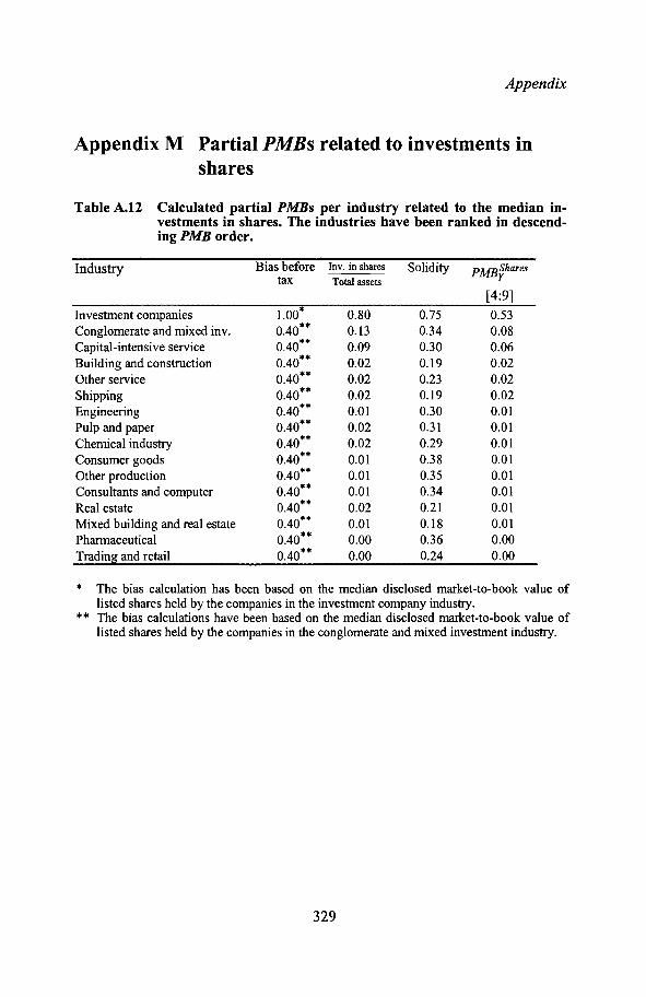
Appendix
Appendix M Partial PMBs related to investments inshares
Table A.12 Calculated partial PMBs per industry related to the median investments in shares. The industries have been ranked in descending PMB order.
Industry Bias before Inv. in shares Solidity PMB~harestax Total assets
[4:9]Investment companies 1.00* 0.80 0.75 0.53Conglomerate and mixed inv. 0.40** 0.13 0.34 0.08Capital-intensive service 0.40** 0.09 0.30 0.06Building and construction 0.40** 0.02 0.19 0.02Other service 0.40** 0.02 0.23 0.02Shipping 0.40** 0.02 0.19 0.02Engineering 0.40** 0.01 0.30 0.01Pulp and paper 0.40** 0.02 0.31 0.01Chemical industry 0.40** 0.02 0.29 0.01Consumer goods 0.40** 0.01 0.38 0.01Other production 0.40** 0.01 0.35 0.01Consultants and computer 0.40** 0.01 0.34 0.01Real estate 0.40** 0.02 0.21 0.01Mixed building and real estate 0.40** 0.01 0.18 0.01Pharmaceutical 0.40** 0.00 0.36 0.00Trading and retail 0.40** 0.00 0.24 0.00
* The bias calculation has been based on the median disclosed market-to-book value oflisted shares held by the companies in the investment company industry.
** The bias calculations have been based on the median disclosed market-to-book value oflisted shares held by the companies in the conglomerate and mixed investment industry.
329

Accounting Information and Stock Prices
AppendixN Partial PMBs related to R&Dexpenditures
Table A.13 Calculated partial PMBs per company related to their medianannual expenditures in R&D. The companies have been ranked indescending PMB order.
Company Industry R&Dexp Expected Solidity PMB:i~,fcode Total assets timelag [3:9]
Astra 6 0.13 7 years 0.36 1.40LKB 6 0.10 " 0.36 1.08Old Pharmacia 6 0.10 " 0.36 1.03Saab-Scania 1 0.08 3.5 years 0.30 0.49Datalogic 9 0.07 " 0.34 0.38Ericsson 1 0.06 " 0.30 0.37Volvo 1 0.06 " 0.30 0.36ProcordialPharma 12 0.05 " 0.34 0.28Inter Innovation 7 0.05 " 0.35 0.25Gambro 7 0.05 " 0.35 0.23Asea 1 0.03 " 0.30 0.21Atlas Copco 1 0.03 " 0.30 0.20Garphytt 1 0.03 " 0.30 0.20Alfa Laval 1 0.03 " 0.30 0.19Sandvik 1 0.03 " 0.30 0.17Old Incentive 12 0.03 " 0.34 0.16Trelleborg 12 0.03 " 0.34 0.16Old Cardo 12 0.03 " 0.34 0.15Nobel 3 0.02 " 0.29 0.12Husqvarna 1 0.02 " 0.30 0.12PLM 1 0.02 " 0.30 0.11Electrolux 1 0.02 " 0.30 0.10SKF 1 0.02 " 0.30 0.09AGA 3 0.01 " 0.29 0.08Iggesund 2 0.01 " 0.31 0.07Euroc 7 0.01 " 0.35 0.06Kockums 1 0.01 " 0.30 0.06SCA 2 0.01 " 0.31 0.05Hoganas 7 0.01 " 0.35 0.05Sydkraft 10 0.01 " 0.30 0.04Modo 2 0.01 " 0.31 0.03
• The bias calculations have been based on an annual real growth rate of 4%, a real rate ofexpected return of 8%, the median solidity for each industry, and the average tax rate forthe period 1967 to 93.
330

Appendix
Appendix 0 Partial PMBs related to deferred taxes
Table A.14 Calculated partial PMBs per industry related to the median deferred tax in unrealized holding gains and untaxed reserves. Theindustries have been ranked in descending PMB order.
Industry
Pharmaceutical
Capital-intensive service
Pulp and paper
Trading and retail
Chemical industry
Consumer goods
Build. and construction
Investment companies
EngineeringConsultants and computer
Other serviceShippingOther production
Mixed build. and real est.
Real estate
Conglomerate and m. inv.
UHG--_.,Total assets
0.44
0.130.12
0.06
0.07
0.18
0.040.41
0.05
0.140.12
0.100.06
0.06
0.10
0.07
UR--_.,Total assets
0.11
0.15
0.14
0.06
0.13
0.130.09
0.00
0.08
0.080.040.02
0.08
0.03
0.01
0.03
Solidity
0.36
0.30
0.31
0.24
0.29
0.38
0.19
0.750.30
0.34
0.230.19
0.35
0.180.21
0.34
DTPMBlndustry
[3: 11]0.51
0.330.27
0.23
0.21
0.200.160.16
0.15
0.150.140.140.13
0.12
0.10
0.09
Definitions of the variables:• Deferred tax in untaxed reserves has been calculated as disclosed untaxed reserves
(variable 121) times the prevailing tax rate. Variable 468 includes each firm's own disclosed estimate of deferred taxes from approximately 1991 and onwards.
331

Accounting Information and Stock Prices
Appendix P Business cycle patterns
Table A.IS A classification of the Swedish industrial business cycle phases infour categories. The business cycle phases are compared at the beginning and end of each possible five- and ten-year value changewindow.
Time Business Business phase in and out in Business phase in and out incycle phase five-year change regressions ten-year change regressions
1967 Recession1968 Up1969 Boom1970 Down1971 Recession1972 Up 1967 -72 R-U1973 Boom 1968 - 73 U-B1974 Down 1969 - 74 B-D1975 Recession 1970 -75 D-R1976 Recession 1971-76 R-R1977 Recession 1972 - 77 U-R 1967-77 R-R1978 Up 1973 - 78 B-U 1968 - 78 V-V1979 Boonl 1974 - 79 D-B 1969 - 79 B-B1980 Down 1975 - 80 R-D 1970 - 80 D-D1981 Recession 1976-81 R-R 1971 - 81 R-R1982 Up 1977 - 82 R-U 1972 - 82 V-V1983 Up 1978 - 83 V-V 1973 - 83 B-U1984 Boom 1979 - 84 B-B 1974 - 84 D-B1985 Boom 1980 - 85 D-B 1975-85 R-B1986 Boom 1981 - 86 R-B 1976 - 86 R-B1987 Boom 1982 - 87 U-B 1977 - 87 R-B1988 Boom 1983 - 88 U-B 1978-88 U-B1989 Down 1984 - 89 B-D 1979 - 89 B-D1990 Down 1985 - 90 B-D 1980 - 90 D-D1991 Recession 1986-91 B-R 1981 - 91 R-R1992 Recession 1987 - 92 B-R 1982 - 92 U-R1993 Up 1988 - 93 B-U 1983 - 93 V-V
332

Appendix
Appendix Q Accounting for acquisitions
Relative frequence of consolidation methods used
100°t'o ....--------------------.oIi!90°t'o80%70°t'o60%50%400/0300/0200/010%
0%I'com-c-
ImPurchase method • "Pooling" method [] Other I
Figure A.l Relative frequency ofchosen consolidation method in the sample offirms.
Annual percentage of the total sample of firmsholding goodwill as a reported asset
60%
50%
40%
30%
200/0
10%
00/0I' m -;: ('t')co co I'm m m m-c- -c- -c- -c-
Figure A.2 Frequency ofthe sample firms that report goodwill as an asset.
333

Accounting Information and Stock Prices
Mean goodwill depreciation as a percentage ofbook value of equity
2.50/0
2.0%
1.5%
0.0%
~
-~1
I 1-1~~ ttl'
~~ I~~~
I 1\ ~ ...... i/i\.1f
~II ,~~
Figure A.3 The unweighted mean of each goodwill reporting firm's annualgoodwill depreciation divided by opening book value ofequity.
Identified annual percentage of goodwill reportingfirms making a large goodwill write-off
60%
400/0
30%
100/0
0% -Mr--f--
I--......It)ex:>0>or-
Figure A.4 The relative frequency ofgoodwill reporting firms that have chosento make a large goodwill write-off.
334

Appendix
Appendix R Ordinary least squares-statisticalconsiderations
In this appendix the following issues will be discussed: complications arising from multicollinearity, heteroscedasticity, autocorrelation and crosssectional dependence as well as the distribution of the residuals, when estimating M.l to M.5 using an OLS approach.
MulticollinearityMulticollinearity means that two or more of the explanatory variables arelinearly correlated. If this correlation is strong it becomes difficult to separate the relative influence on the dependent variable of the different collinear variables. A possible consequence is that regression coefficients showvalues that depart largely from population values (even show the wrongsign) and/or are insignificant even when the combined explanatory power ishigh. A number of tests have been performed to establish the extent towhich the regression coefficients might be affected by collinearity betweenthe variables. The Pearson correlations between the explanatory variables inthe pooled samples have been calculated and are presented in table A.16.
Table A.16 The Pearson correlation between the explanatory variables in thepooled full sanlples.
Panel A: Level modelM.2 PMB) N
Panel B: Change modelsJ-year
M.4& MI M·PMB
M.5 P P
2-year
!:JU M·PMB
P P
5-year
!:JU M·PMB
P P
JO-year
!:JU tJJ . PMB
P P
MP
t:JU
P
-0.20 0.94
-0.20
0.03 0.91
0.01
0.20 0.85
0.14
0.41 0.83
0.32
/1b =bj,t+k - bj,t
P Pj,t
335
M· PMB (bj,t+k -bj,t)' PMBj
P Pj,t

Accounting Information and Stock Prices
Edlund (1995) states that a correlation between two explanatory variables inexcess of 0.8 (absolute value) is a sufficient but not necessary condition fortIle presence of collinearity (correlation exceeding 0.5 between several variables may also be an indicator of multicollinearity). According to these criteria, it appears that collinearity should not cause any general problems forthe level specification. Neither does the correlation between the change inbook value of equity and the change in residual earnings variable of thechange regression M.4 seem to be alarmingly high for any of the windowlengths. However, the correlation between change in book value of equityvariable and the change in book value of equity times the estimated PMBvariable is (perhaps not surprisingly) strong. This unfortunately makes theinterpretation of the regression coefficients of specification M.5 suspect. Toavoid the problems of multicollinearity of regression specification M.5,without excluding the effect of different PMBs, the following regressionn10del has been specified. Here, the measurement bias has beel1incorporated into the value creation variable. The slope coefficient ei inM.5' is expected to equal 1.0, given valid estimates of the measurementbias.5
M.5'
When running the actual regressions, the collinearity diagnostic, known asthe condition index has further been evaluated for several sub-samples. According to Edlund (1995, p. 80), a condition index between 10 and 30 indicates collinearity growing from mild to strong. A condition index exceeding30 indicates severe collinearity. With the exception of specification M.5, noalarmingly high condition indexes have been observed.
5 The correlation between the explanatory variables of M.5' is very similar to the variables ofM.4.
336

Appendix
Heteroscedasticity
An assumption of the classical linear regression model is that the disturbance terms appearing in the regression function are homoscedastic, that is,that they all have the same variance independent of the value of the explanatory variables. If this is not the case, the ordinary t- and F-test of theregression will not be valid. A comn10n approach in the MBAR literaturehas been to check for the presence of heteroscedasticity using the generaltest proposed by White (1980). When heteroscedasticity cannot be rejected,it has been common to use the heteroscedasticity-consistent standard errorssuggested by White (1980) when calculating t-statistics. In a methodologicalarticle evaluating the pros and cons of return and price models, Kothari andZimmerman (1995) note that price n10dels more frequently reject tests ofhomoscedasticity than return models.6 They further note that this problem ismost severe for undeflated price models. In the present study, price has beendeflated by book value of equity, and therefore the most important source ofheteroscedasticity should have been eliminated.
Utilizing the test proposed by White (1980), homoscedasticity cannot berejected for either the level or the change specification for the full pooledsample. Unadjusted t-statistics will therefore generally be used as a descriptive metric. However, t-statistics utilizing White's heteroscedasticityconsistent standard errors have also been calculated for a large number ofthe regressions presented in the next two chapters.
Autocorrelation and cross-sectional dependence
"The term autocorrelation may be defined as correlationbetween members of observations ordered in time [as in timeseries data] or space [as in cross-sectional data]. "
Gujarati(1988,pp.353)
In the presence of autocorrelation or cross-sectional dependence betweenthe error terms, an OLS regression can still provide unbiased coefficientestimates, but the cross-sectional dependence in the data may generate anunderestimation of the standard errors of the regression coefficients. This in
6 This was further predicted to be the case by Christie (1987).
337
12 RUllsten

Accounting Information and Stock Prices
tum implies that the standard norm for judging the significance of t-valuesis violated.7 Bernard (1989) notes:
"In tests involving slope coefficients in cross-sectional regressions (e.g., most valuation/information content studies), the degree ofbias is difficult to predict, but it is more likely to be serious when long return intervals (monthly, quarterly, or annual)are used. Unfortunately, these happen to be the contexts where itis most difficult to deal with the issue. ... in some cases the researcher may have no choice but to add a note of caution whendrawing conclusions. "
Bernard (1989, p. 104)
In this study, regressions are mainly run in cross-section, but also in pooledcross-section and time-series. Autocorrelation resulting from the way observations are ordered in time should not cause severe problems in this study.However, cross-correlation in space may result from consequences of, forexample, fluctuations in the business cycle, inflation rate changes, andchanged accounting practice. Problems related to these issues have beentackled in two ways in this study: i) inferences are largely made from themean of estimated coefficients across all years, ii) a number of regressionsthat explicitly attempt to control for a potential source of cross-correlationare evaluated. Nevertheless, 100 percent precise judgments of statisticalsignificance are difficult to generate from the regression specifications suggested in this study. As a consequence, estimated t-statistics have to beviewed mainly as descriptive statistics.
The probability distribution of the residualsAn assumption of normally distributed error terms is not needed to obtainbest linear unbiased estimators (BLUE) of the regression coefficients.8
However, to enable inferences to be drawn regarding the true level of thecoefficients, knowledge of the probability distribution of the error terms isessential.
7 See Bernard (1987).8 See Gujarati (1988, p. 88) and Edlund (1995, p. 126).
338
Appendix
For the full pooled sample, a hypothesis of normally distributed error termscan be rejected. This appears to be driven mainly by the presence of toon1any extreme observations (too many large and too few small market-tobook value premium observations in the level specification). As these extreme observations may have an undue influence on the regression results,the regressions will also be run excluding the extreme observations.
Interpreting the R2 and testing for significant differences
The explanatory power (R2) or adjusted explanatory power (R2) of theregressions in this study are of interest in several dimensions. First, it is ageneral indication of how much of the variation in the market-to-book valuepremium (in the level specifications) can be explained by expected residualreturn (M.1) and subsequently by adding the PMB variable (M.2). Sin1ilarly,the level of explanatory power is interesting as an indicator of the extent towhich the value change observed on the stock market can be explained byaccounting measures (M.3 to M.5). Whether or not the adjusted R2 increaseswhen an additional explanatory variable is included in a regression is anindication of the marginal explanatory power of the added variable.
The relative explanatory power for different sub-groups of firms (grouped,e.g. according to a firm-specific characteristic or the choice of particularaccounting method) is also of interest. However, the interpretation of different levels of R2 for different sub-samples of firms or periods is not uncomplicated. Can the change in R2 really be attributed to the specific treatment?Is the change significant?
Based on the properties of R2 observed by Cramer (1987), Harris, Lang andMoller (1994) constructed a variable to test for differences in R2 betweentwo different sub-samples. A Z-statistic that is approximately standard normal in large samples was computed as follows:9
9 See Harris, Lang and Moller (1994) p. 198.
339

Accounting Information and Stock Prices
The estimated level of variance (02) depending on the san1ple size, the number of regression coefficients and the underlying true association generatedvia sin1ulation in Cramer (1987) was used. After having derived theexpected mean and standard deviation ofR2, Cramer concluded:
tiThe mean ofR2 converges to its probability limit from above,and in this sense it has an upward bias which can be substantialin small samples. In this respect R 2 is superior. The standarderrors show, however, that for sample sizes of up to 40 or 50either measure is a very unreliable statistic. "
Cramer(1987,p.253)
Using the indicator suggested by Harris, Lang and Moller (1994) and thevariance estimations from Cran1er (ibid.)10 calculations can be made thatshow that to obtain a Z-statistic in excess of, for example, 2.0011 the relativeabsolute difference between two estimated R2s must at least amount to approximately 20% for sample sizes of 20 observations, to 15% for samplesizes of 50 observations, to 10% for sample sizes of 100 observations, andto approximately 7% for sample sizes of 200 observations. (See table belowfor n10re details.)
Table A.17 The necessary difference in R2 in order to obtain a f"score=2.00for different sample sizes and different levels of fi..J ' given thecalculated standard deviations in Cramer (1987, table 1) and aregression with two explanatory variables.
Al2 = 66.7%
n A~ - f?i ~ Z =2.00
20 20.8°A»30 17.2%40 15.2%50 13.6%
100 9.8%150 8.1%200 6.3%
f?~ = 50.0%
f?~ - f?i ~ Z =2.00
23.8%19.9%17.4%15.8%11.5%9.5%7.5%
f?~ =33.3%
f?~ - Ai ~ Z = 2.00
20.9%17.8%15.7%14.3%10.5%8.7%6.8%
10 The variance ofR2 decreases most notably as the sample size increases.11 Implying approximately a 5 percent significance level for a two-tailed test.
340

Appendix
The actual observed R2 differences in the Chapters 7 and 8 can be evaluatedwith these estimated values in mind. However, given the sensitivity ofR2 to,for example, the presence of outliers, these calculations of necessary R2differences should only be viewed as crude indications of the minimum necessary difference.
341
J3 Runsten

Appendix S M.2 regressions results
Table A.18 Summarized pooled M.2 regressions excluding all observations when the dependent variable(the market-to-book value premium) exceeds 4.
Sample characteristics a PI /32 li 2 nFull sample 0.39 (9.9)** 4.07 (17.6)** 0.58 (8.1)** 14.8% 2650
Profit rec. = Continuous 0.36 (8.1)** 4.98 (15.8)** 0.42 (5.4)** 22.6% 1 666Profit rec. = Discrete 0.03 (0.4) 3.49 (9.6)** 1.73 (10.1)** 14.0% 984
ROE hist. = Stable 0.39 (6.5)** 6.11 (9.0)** 0.59 (6.1)** 12.7% 974ROE hist. = Intennediate 0.36 (4.3)** 4.91 (10.0)** 0.64 (4.3)** 18.2% 664ROE hist. = Turbulent 0.63 (5.4)** 3.05 (9.0)** -0.01 (-0.1) 16.9% 527
Profit rec. = Continuous &ROE hist. = Stable 0.38 (5.7)** 10.36 (13.7)** 0.45 (4.8)** 33.1% 611ROE hist. = Intennediate 0.30 (3.3)** 6.49 (11.1)** 0.66 (4.0)** 31.1% 416ROE hist. = Turbulent 0.89 (6.0) ** 2.89 (6.6)** -0.71 (-2.5) 16.9% 331
E[GPF] = Low 0.40 (2.4) * 2.55 (5.0)** 0.29 (0.9) 8.3% 351E[GPF] = Medium 0.39 (9.7)** 5.07 (14.4)** 0.58 (8.1)** 13.0% 2 170E[GPF] = High 0.21 (1.0) 5.77 (3.6)** 1.01 (2.5)** 13.7% 129
Homogenized sample 0.31 (5.6)** 7.94 (13.2)** 0.49 (5.9)** 26.2% 924
I-statistics (with White (1980) homoscedasticity-consistent standard errors) in parenthesis, a two-sided test is used for intercepts and a onesided test for the slope coefficients.* Significant at 0.01 ~ a ~ 0.05** Significant at a ~ 0.01

Appendix
Appendix T Earnings expectations from a businessmagazine for a sDtal1 group of companies
Affarsvarlden's earnings forecasts are not found in any accessible database,and therefore manual extraction from the actual magazines is required. Asmall group of 16 continuous profit recognition firms that have been listedfor the whole period studied was selected. 12 These 16 firms are larger thanthe average firm in the study and belong to six different industries. 13
Market value is measured at the end of March every year. To be consistent,this should also be the date for the measurement of earnings expectations.From early 1992 and onwards, this causes no problems as Affarsvarlden hassince then published forecasts of earnings per share two years ahead. Before1992 (with only a one-year ahead estimate), Affarsvarlden had generally notupdated its forecast for the following year at the end of March. Instead theearliest possible published forecast of next period earnings per share hasbeen chosen. 14
In order to translate the earnings per share prediction into a return on equityprediction, the earnings per share forecast has been multiplied by the number of shares outstanding and divided by the book value of equity accordingto the definition generally used in this study (see Section 4.2.1.3). This ROEprediction has then been transformed into a residual return prediction usingthe same firm and time specific p and ras before (see Section 4.4.3, equation 2:35).
Table A.19 shows the annual results of M.2 regressions for this small sample of firms. Panel A shows the results when the standard prediction approach, based on historical ROE, has been utilized; panel B presents theresults generated when the earnings forecasts from Affarsvarlden is utilized.
12
13
14
These 16 firms are: AGA, Astra, Atlas Copco, Eldon, Electrolux, Ericsson, ESAB,Euroc, Garphyttan, MoDo, Sandvik, SCA, SKF, Stora, Sydkraft, and Volvo. An important caveat is, of course, that the small sample size also makes the annual regressionsespecially sensitive to individual extreme observations.9 engineering firms, 3 paper & pulp firms, 1 firm from pharmaceuticals, chemicals,other production and capital-intensive service, respectively.For some firms with late publication of the annual report this means mid May, but formost of the firms it means sometime during April.
343

Accounting Information and Stock Prices
Table A.19 Annual regression results using regression specification M.2.
erformance
YEAR a PI P2 li2 n
1984 -0.40 (-1.9) 3.56 (2.0) 0.94 (3.7) 52.1% 161985 -0.28 (-1.3) 5.02 (2.5)* 1.35 (4.9)** 68.4% 161986 -0.43 (-1.1) 6.02 (1.2) 2.15 (5.1)** 69.5% 161987 -0.08 (-0.3) 8.30 (1.9)* 1.45 (3.9)** 57.6% 161988 0.24 (0.8) 5.85 (2.2)* 1.58 (4.3)** 56.4% 161989 -0.82 (-1.9) 4.21 (0.7) 2.95 (5.8)** 68.9% 161990 -1.01 (-2.6)** 8.15 (2.4)* 3.14 (7.4)** 88.3% 161991 -1.09 (-1.6) 4.26 (1.2) 3.15 (4.9)** 83.1% 161992 -0.37 (-0.6) 5.81 (1.9)* 2.25 (3.7)** 77.2% 161993 0.28 0.3 4.52 1.7 1.36 2.3 ** 63.7% 16
Panel B: E RO based on forecasts
YEAR a PI li 2 n
1984 -0.03 (-0.2) 6.61 (3.3) (3.7) 65.7% 161985 0.07 (0.3) 6.52 (3.1)** (5.0)** 72.8% 161986 0.41 (1.1) 16.04 (3.8)** (6.0)** 84.1% 161987 0.28 (0.8) 10.58 (2.3)* (4.3)** 62.2% 161988 0.50 (1.7) 9.82 (2.6)* (4.3)** 60.6% 161989 -0.16 (-0.5) 13.82 (4.7)** (7.7)** 88.0% 161990 -0.46 (-1.2) 10.98 (3.8)** (6.3)** 91.9% 161991 -0.39 (-0.9) 8.42 (3.8)** (6.0)** 91.1% 161992 -0.14 (-0.3) 7.54 (2.8)** (3.7)** 81.8% 161993 0.45 1.2 8.36 3.3 ** 2.3 * 75.9% 16
I-statistics in parenthesis, a two-sided test is used for intercepts and a one-sided test for theslope coefficients.
* Significant at 0.01 ~ a ~ 0.05** Significant at a ~ 0.01
Figure A.5 and A.6 visualize the difference between the ]i2 and the estimated PI - coefficient with the two different return on equity prediction procedures.
344

Appendix
Adjusted R2 with differentestimation procedures for ROE
1000k
800k
600/0
400/0
20%
0%
~(j)~
lOex:>0)~
coex:>(j)~
r--ex:>en~
ex>ex:>(j)~
enex>(j)~
oenen~
m(j)~
N(j)0)~
('t)0)0)~
I· ·.. ··E[ROE] based on previous year 0 E[ROE] from Affarsvarlden I
Figure A.5 The]i2 for the annual M.2 regressions for a 16-company sampleusing two estimation proceduresfor nextperiod's ROE.
The GPF (~1) with differentestimation procedures for ROE
18 -r-------------------------....16 -I--------I::::,~------------------_I14 -I----------.f---~-----__:~----------_I12 -I------I---~k-----~~--~--------_I10 -I----__:#-----~~-___rvc_--------3IlIlo;;;::__------_1
8-.-------r-----:-r'~=___._:__-----___.___JI~-------=---1IiiiiiiiiiiiIi~;;;;;iijiiiiiii".,.-"'Y
6:y:-...:~_"'"1IL.---~~----.LA_-------1----__=_A_;;;______-_I
4 .... ~
2 -1----------------------------11
O........--+__---+--~--_+_--_+__--+__-__+--~-- .....1984 1985 1986 1987 1988 1989 1990 1991 1992 1993
\. • .. • • E[ROE] based on previous year e E[ROE] from Affarsvarlden I
Figure A.6 The estimated annual growth persistence factor (p1) for annual M.2regressions for a 16-company sample using two estimation procedures for next period's ROE.
345

Accounting Information and Stock Prices
It is striking that the prediction procedure used by the business magazineclearly dominates the more mechanical historical performance-based prediction approach, both in terms of consistently higher explanatory powerand in terms of a higher frequency of significant GPF coefficients. It is notable, however, that both specifications yield high explanatory power forthis sample of firms during the period studied (a mean of 68.5% vs. 77.4%),and that the difference in explanatory power is rather small and quite constant over time.
Another notable result concerns the level of the estimated PI coefficients.Relying on Affarsvarlden's earnings forecasts, the PI coefficients are higherevery single year and on average almost 10 (as compared to 5.6 when themain earnings prediction procedure is used). Given the economic interpretation of this coefficient, a value of 10 indicates that the market expects ahighly persistent abnorn1al performance from this group of companies. Thesmall sample size makes it difficult to assess if the different variability inthe slope coefficients over time is the result of individual extreme observations or if it is related to a more fundamental underlying cause.
These results indicate that Affarsvarlden's earnings forecasts constitute abetter description of the earnings expectations on the stock market than thesimple estimation procedure utilized in main part of this study. However, itis encouraging to observe in figure A.5 the close covariability over the yearsbetween the level of explanatory power. This indicates that the two returnon equity prediction procedures seem to capture essentially the same phenomena. The mechanical historic performance method, however, seems tobe somewhat more 'noisy'.
In order to evaluate if the varying explanatory power of M.2 (observed inSection 7.3.1) with regard to the phases of the business cycle remains whenAffarsvarlden's earnings forecasts are used figure A.7 is provided.
346

Appendix
Adjusted R2 in different business cycle phases
.•... ·e··- ._ .. _..100%
80% oI"f).
60%R2
400k
200/0
OOko0)0)~
70
60 5...50 i
N
40S~
30 fJ...20 5
en10 ~
0('t')0)0)~
I· ... ·.E[ROE] from Affarsvarlden ---Resource utilization I
Figure A. 7 The adjusted explanatory power (li. 2) for each annual estimation ofM.2 for the 16-company sample using ROE forecasts fromAfflirsvlirlden, combined with an index ofthe Swedish industrial resource utilization.
The figure clearly shows that the negative association between the explanatory power of M.2 and the phase of the business climate remains whenAffarsvarlden's earnings forecasts are used. The adjusted R2 is apparentlylower during and around the boom periods of the economy, and higher during and around a recession.
347

Accounting Information and Stock Prices
Appendix U Accounting for depreciation
Table A.20 Accounting for depreciation: Pooled regression results usingregression specification M.2 and the homogenized sub-sampleof firm-years starting from the nine industries with firmswhere most depreciable assets are held.
Panel A: 1967-80
1967-80 a PI /32 ]i2 nAll firms -0.22 (-6.0)** 5.18 (12.2)** 0.45 (9.3)** 36.4% 409
Non-disclosure -0.11 (-1.0) 5.41 (6.7)** 0.40 (1.9)* 23.1% 153Open Disclosure -0.46(-10.7)** 3.39 (7.0)** 0.56 (13.9)** 62.5% 164
Panel B: 1971-78
1971-78 a /31 /32 ]i2 n
All firms -0.18 (-3.9)** 5.17 (9.1)** 0.44 (6.9)** 31.4% 275
Non-disclosure --0.02 (-0.2) 5.26 (5.2)** 0.29 (1.1) 18.7% 110Open Disclosure --0.45 (-7.8)** 3.31 (4.7)** 0.54 (10.5)** 60.4% 94
Panel C: 1975-76
1975-76 a PI P2 ]i2 n
All firms --0.06 (-0.7) 5.19 (4.9)** 0.31 (2.8)** 31.3% 65
Non-disclosure 0.07 (0.3) 5.19 (2.8)** 0.32 (0.7) 19.7% 25Open Disclosure -0.41 (-3.0)** 2.94 (1.8)* 0.48 (4.9)** 62.9% 21
Panel D: 1970-74
1970-74 a PI {32 li 2 n
All firms --0.20 (-3.2)** 4.98 (6.3)** 0.43 (4.9)** 24.10/0 182
Non-disclosure -0.13 (-0.8) 5.77 (5.0)** 0.40 (1.3) 20.6% 96Open Disclosure -0.37 (-3.8)** 2.92 (2.3)* 0.45 (4.4)** 39.7% 30
Panel E: 1975-78
1975-78 a PI /32 li 2 nAll firms --0.17 (-2.7)** 5.55 (7.6)** 0.44 (5.8)** 43.3% 124
Non-disclosure 0.15 (0.7) 4.93 (3.3)** 0.14 (0.4) 22.6% 32Open Disclosure --0.49 (-5.9)** 3.21 (3.2)** 0.58 (9.4)** 65.1% 66
t-statistics in parenthesis, a two-sided test is used for intercepts and a one-sided test for theslope coefficients.
* Significant at 0.01 ~ a ~ 0.05** Significant at a ~ 0.01
348

Appendix
Appendix V Accounting for associated companiesThe mean value of the dependent and the independent variables with thedata grouped according to different accounting methods for associated conlpanies.
Market-to-book valuepremium
E[RR]
5°k +-- ---1
10% ....,...- ---.,
19871986
0% «
.4::~ •••••••••••••: •••••••••••••~~
-5% +------------1
-100/0 +--- +- ---1
1985
2.0...,...---------_-..,
1.5 ~ ~::,
~:~ t7.-<_. " _ "0.0 +-------------1
-0.5 +-------------1
-1.0 -+-- ~----~
1985 1986 1987
I ...A· •• Cost rrethod --<>-- Equity rrethod 1 I ... A· •• <Ast rrethod --<>-- Equity rrethod 1
Figure A.8 The mean market-to-book value premium and the mean EIRR] forthe companies using the cost method versus companies using theequity method.
PMB
1.00 -r------------,0.75 +-----=~~:::::::::::~___==_-~
19871986
0.25 +-----------i
0.00 -+-- --+ ~
1985
I·· ·A··· <Ast rrethod --<>-- Equity rrethod I
Figure A.9 The mean PMB for the companies using the cost method versuscompanies using the equity method.
349

gG
rAGPFjM
SYMBOLS AND ABBREVIATIONS
The symbols and abbreviations for different variables, parameters andindexes used in this study fall into four categories:
A. Symbols used when specifying the valuation model (chapter 2)B. Symbols used in the regression specifications (chapter 2, 6, 7 and 8)C. Symbols used for accounting measurement bias calculations (chapter 3)D. Other abbreviations
The list below contains short descriptions of each symbol, groupedaccording to these four categories. Note that additional symbols have beenused in restricted sections of this study, and are only described in thesesections.
A. Symbols used in specifying the valuation modela Superscript for abnormal performanceB Book value of equityb Book value of equity per share(b) Superscript for biased accounting(u) Superscript for unbiased accountingfJ A risk parameterD DividendsEt(..) Expectations at the end of time t
Denotes a stochastic variableAn unpredictable disturbance termGrowth rate1 plus the growth rateAnnual return measurement biasA fading factor of abnormal returnEquity Growth earnings Persistence FactorSubscript for firmMarket value

Accounting Information and Stock Prices
p Market value per sharem A time indexN New issuesNT Net transactions to ownersPMB Permanent measurement biasr Risk-free rate of interestp Cost of equity capital including a risk premiumRI Residual incomeROE Return on owners' equityrp Risk premiumRR Residual returns A time indext Subscript for time; when related to a flow variable, such as
return on equity, describes a time period (t-1, t), whenrelated to a stock variable, such as price or book value ofequity, t refers to the end of the time period.
T A number ofperiods into the futureT A time indexV Economic valuex Earnings
B. Symbols used in the regression specificationsEstimated intercept in the level models (M.1 and M.2)Estimated slope coefficient for E[RR]Estimated slope coefficient for the PMBEstimated intercept in the change models (M.3 to M.5)Estimated slope coefficient for cl1ange in book value ofequityEstimated slope coefficient for change in E[R1]Estimated slope coefficient for change in book value ofequity times the PMBEstimated slope coefficient for change in book value ofequity times (1 plus the PMB) in regression model M.5'
c. Symbols used for accounting measurement bias calculationsA Assetacc[...] The accumulated value of an asset typeAP Acquisition price
351

Lt8DThI
I.A.kLnOffpq
*r
rd,at(r)t"
T.A.TAUHGUR¢1](J
rp
Symbols and Abbreviations
Annual changeAnnual real growth rate in the level of expendituresDeferred taxThe number ofyears until an investment pays offAnnual expenditures creating an intangible assetAnnual value changeSuperscript for intangible assetsSubscript for asset typeLiabilityThe age of an asset (0 years to N years)Off-balance sheet itemNumber ofperiods until a tax liability is expected to be paidThe annual percentage growth rate in number of acquiredunitsA real discount rateCost of debt after taxSuperscript for reported valueThe tax rateSuperscript for tangible assetsTotal assetsUnrealized holding gainUntaxed reservesSubscript for intangible asset typeSubscript for type of off-balance sheet itemSubscript for liability typeSubscript for type of deferred tax liability
D. Other abbreviationsABL Companies ActBFL Accounting ActBFN Accounting BoardCPI Consumer Price IndexFAR Swedish Institute of Authorized Public AccountantsNBK Industry and Commerce Stock Exchange CommitteeRR the Swedish Financial Accounting Standards CouncilSFF Swedish Association for Financial Analysts
352

REFERENCES
"Att skilja vinnare fran forlorare", 1987, "En introduktion till Affarsvarldens modell for aktievardering och en presentation avAffarsvarldens placeringsindikatorn" 4:th edition, Affarsvarldens Forlag AB
Ali, Ashiq and Paul Zarowin, 1992, "Permanent versus transitory components of annual earnings and estimation error in earningsresponse coefficients", Journal ofAccounting and Economics,# 15, pp. 249-264
Atlgelin, Ken and L. Peter Jennergren, 1994, "Partner leasing in Sweden",EFI Research Paper No. 6547, Stockholm School ofEconomics, October
Ball, Raymond J. and Philip Brown, 1968, "An Empirical Evaluation of Accounting Income Numbers" Journal ofAccounting Research,Autumn,pp.159-78
Ball, Raymond J. and Ross L. Watts, 1972, "Some Time Series Properties ofAccountitlg Income" Journal ofFinance, June, pp. 663-682
Ball, Ray and George Foster, 1982, "Corporate Financial Reporting: AMethodological Review of Empirical Research" Journal ofAccounting Research, Vol. 20 Supplement, pp. 161-234
Beaver, William H., 1968, "The Information Content of Annual EarningsAnnouncements" Journal of Accounting Research, Supplement
Beaver, William H., 1970, "The Times Series Behavior of Earnings" Empirical Research in Accounting: Selected Studies, Supplementto Journal ofAccounting Research, #8 pp. 62-89
Beaver, William, H., 1981, "Financial Reporting: An Accounting Revolution" Prentice-Hall
Beaver, William, H., 1989, "Financial Reporting: An Accounting Revolution" Second Edition, Prentice-Hall International Edition

Accounting Information and Stock Prices
Beaver, William H., Kettler, P and M. Scholes, 1970, "The Association between Market Determined and Accounting Determined RiskMeasures" Accounting Review, October, pp. 654-82
Beaver, William H., R. Clarke and W. Wright, 1979, "The Association between Unsystematic Security Returns and the Magnitude ofEarnings Forecast Errors" Journal of Accounting Research,Autunrrn,pp.316-340
Beaver, Willian1 H., R. Lambert and D. Morse, 1980, "The InformationContent of Security Prices", Journal of Accounting andEconomics, March, pp. 3-28
Bernard, Victor L., 1987, "Cross-Sectional Dependence and Problems inInference in Market-Based Accounting Research" Journal ofAccounting Research, Vol. 25 No.1 Spring, pp. 1-48
Bernard, Victor L., 1989, "Capital Markets Research in Accounting Duringthe 1980's: A Critical Review", in Thomas Frecka (ed.), "TheState of Accounting Research as We Enter the 1990's", pp.72-120, Urbana-Champaign: University of Illinios
Bertmar, Lars och Goran Molin, 1977, "Kapitaltillviixt, Kapitalstruktur ochRiintabilitet - En analys av svenska industriforetag" EFI
Blume,1970, "Portfolio Theory: A Step Towards Its Practical Application",Journal ofBusiness, April
Bonbright, J.C., 1937, "The valuation ofproperty", Vol. I-II, New YorkBowen, R.M., 1981, "Valuation of Earnings Components in the Electric
Utility Industry" The Accounting Review, JanuaryBrief, Rich.ard P. and Raef A. Lawson, 1992, "The Role of the Accounting
Rate of Return in Financial Statement Analysis", TheAccounting Review, April, pp. 411-426
Brooks, L. and D. Buckmaster, 1976, "Further Evidence of the Time SeriesProperties of Accounting Income" Journal of Finance, December, pp.1359-1373
Brooks, L. and D. Buckmaster, 1980, "First Differences Signals andAccounting Income Time Series Properties" Journal of Business Finance and Accounting, # 7,3 pp. 437-455
Brown, L., PP. Griffin, R. Hagerman and M. Zmijewski, 1984, "The Existence and Potential Sources of Analyst Forecast Superiority"working paper State University ofNew York at Buffalo
354

References
Brown, L.D. and M.S. Rozeff, 1979, "Univariate Time-Series Models ofQuarterly Accounting Earnings per Share: A Proposed Model"Journal ofAccounting Research, Spring, pp. 179-189
Brown, Philip, 1968, "Some Aspects of Valuation in the Railroad Industry" Ph.D. dissertation, University of Chicago
Bublitz, Band M. Ettredge, 1989, "The Information in Discretion Outlays:Advertising, Research and Development", The AccountingReview, No. 64, pp.108-124
"Business Tendencies Surveys", 1975-94, National Institute of EconomicResearch, Konjunkturinstitutet, Stockholm
Chen, Nai-fu, Richard Roll and Stephen Ross, 1986, "Economic Forces andthe Stock Market", Journal ofBusiness, 59, pp. 383-403
Christie, Andrew A., 1987, "On Cross-sectional Analysis in AccountingResearch" Journal ofAccounting and Economics # 9
Clinebell, John M., D.R. Kahl and J.L Stevens, 1994, "Time-series Properties of the Equity Risk Premium", The Journal of FinancialResearch, No.1 Spring, pp. 105
Cook, T.D. and D.T. Campbell, 1979, "Quasi-Experimentation: Design &Analysis Issuesfor Field Settings", Chicago: Rand McNally
Copeland, Thomas E. and J. Fred Weston, 1988, "Financial Theory andCorporate Policy" Third Edition, Addison-Wesley PublishingCon1pany
Copeland, Tom, Tim Koller and Jack Murrin, 1991, "Valuation: Measuringand Managing the Value of Companies", McKinsey & Company, Inc. John Wiley & Sons
Cramer J.S., 1987, "Mean and Variance of R2 in Small and ModerateSamples", Journal ofEconometrics, # 35, pp. 253-266
Damodaran, Aswath, 1994, "Damodaran on Valuation--Security Analysisfor Investment and Corporate Finance", John Wiley & Sons
Easton, Peter and Trevor Harris, 1991, "Earnings as an Explanatory Variable for Returns", Journal of Accounting Research, Spring,pp. 19-36
Easton, Peter, Trevor Harris and James Ohlson, 1992, "Aggregate accounting earnings can explain most of security returns: The case oflong return intervals", Journal ofAccounting and Economics,vol. 15 pp. 119-142
Edlund, Per-Olav, 1995, "SPSSfor Windows - Multipel regressionsanalys"Studentlitteratur, Lund
355

Accounting Information and Stock Prices
Edwards, Edgar O. and Philip W. Bell, 1961, "The Theory and Measurelnent ofBusiness Income" The University of California Press
Engshagen, Ingrid, 1987, "Finansiella nyckeltal for koncern versus koncernbolag - En studie om finansiella ma1tal" Opubliserad licentiatavhandling: EFI, Stockholm
Fama, Eugene and James MacBeth, 1973, "Risk, Return and Equilibrium:Empirical Tests", Journal ofPolitical Economy, 81, pp. 607636
Fama, Eugene and Kenneth French, 1992, "The Cross-Section of ExpectedStock Returns", The Journal ofFinance, June, pp. 427-465
FASB, 1976, Tentative Conclusions on Objectives ofFinancial StatementsofBusiness Enterprises
FAR, 1965-78, "FARs: Ledamotsforteckning Stadgar Rekommendationer", Foreningen Auktoriserade Revisorer
FAR, 1979-95, "FARs Samlingsvolym", Foreningen Aulctoriserade Revisorer
FINDATA, 1985, "Findatasystemet - Anvandam1anual" Findata FinansiellInformation AB, version March
FINDATA, "Trust", SIX ABFisher, J., 1906, "The Nature ofCapital and Income", MacmillanForsgardh, Lars-Erik och Krister Hertzen, 1975, "Information Forviint-
ningar och Aktiekurser - En studie av den svenska aktiemarknaden" EFI, Stockholm
Foster, George, 1986, "Financial Statement Analysis" 2nd edition, Prentice-Hall
Francis, Jennifer, Per Olsson and Dennis R. Oswald, 1997, "Comparing theAccuracy and Explainability of Dividend, Free Cash Flow andAbnormal Earnings Equity Valuation Models", Draft of working paper, SSE
Fredriksson, Goran, Svante Johansson och Henrik Neuhaus, 1983,"Matematikfor ekonomer" Studentlitteratur, Lund
Freeman, R.N., J.A. Ohlson and S.H. Penman, 1982, "Book Rate-of-Returnal1d Prediction of Earnings Changes: An Empirical Investigation" Journal ofAccounting Research, Autumn, pp. 639-653
Freeman, Robert N., and Senyo Y. Tse, 1992, "A Nonlinear Model of Security Price Responses to Unexpected Earnings" Journal ofAccounting Research, Autumn, pp. 185-209
356

References
Frennberg, Per and Bjorn Hansson, 1991a, "Risk and return on Swedishstocks: 1919-1989", Skandinaviska Enskilda Banken Quarterly Review, # 1-2, pp. 15
Frennberg, Per and Bjorn Hal1sson, 1991b, "Testing the Random WalkHypothesis on Swedish Stock Prices: 1919-1990", Lund University: working paper series: 1991/10
Fruhan, Jr. William E., 1979, "Financial Strategy--Studies in the creation,transfer and destruction of shareholder value" Richard D.Irwin, INC.
Gordon, Myron J. 1959, "Dividends Earnings and Stock Prices" Review ofEconomics and Statistics, May pp. 96-105
Gordon, Myron J. 1962, "The Savings Investment and Valuation of aCorporation" The Review of Economics and Statistics,Februa~,pp.37-51
Granger, C. W. J. 1972, "Empirical Studies of Capital Markets: A Survey"In G. P. Szego and K. Shell, editors, Mathematical Methods inInvestment and Finance, Amsterdam, North-Holland, pp. 469519
Green, J. Peter, Andrew W. Stark and Hardy M. Thomas, 1996, "UKEvidence on the Market Valuation of Research and Development Expenditures", Journal of Business Finance &Accounting, Vol. 23 March, pp. 191-216
Greene, William H., 1993, "Econometric Analysis", Macmillan PublishingCompany, New York
Gujarati, Damodar N., 1988, "Basic Econometrics", Second Edition,McGraw-Hill International Editions
Hall, B, 1993, "The Stock Market Value of R&D Investment during the1980s", American Economic Review, No. 83, pp. 259-264
Hanner, PerV. A., 1953, "Arsredovisningen ipraktiken"FFI StockholmHanner, Per V. A., 1964, "Arsredovisningen i praktiken II" FFI StockholmHanner, Per V. A., 1980, "Nagra milstolpar i redovisningens utveckling
under 1900-talet i Sverige" Unpublished document,Handelshogskolan i Stockholm
Harris, Trevor S., Mark Lang and Hans Peter Moller, 1994, "The ValueRelevance of German Accounting Measures: An EmpiricalAnalysis" Journal of Accounting Research, Vol. 32 No.2Autunrrn,pp.187-209
357

Accounting Information and Stock Prices
Hendriksen, Eldon S., 1982, "Accounting Theory", Fourth edition, RichardD. Irwin, Inc. Homewood, Illinois
Ibbotson, R. and G. Singquefield, 1989, "Stocks, Bonds, Bills and Inflation, 1989 Yearbook" Ibbotsons Associates, Chicago
Ijiiri, Yiji, 1967, "The Foundations of Accounting Measurement: AMathematical, Economic and Behavioral Inquiry", Engle,vood Cliffs, N.j.: Prentice-Hall, Inc.
Johansson, Sven-Erik, 1959, "Metoder for viirdering av foretag enligtforetagsekonomisk litteratur", Manuscript, Stockholm Schoolof Economics
Johansson, Sven-Erik, 1961, "Skatt-Investering-Viirdering", EFI, Stockholm
Johansson, Sven-Erik, 1995, "Foretagets lonsamhet, jinansiering ochtillviixt - Mal, samband och miitmetoder", Studentlitteratur,Lund, 2:nd edition
Johansson, Sven-Erik and Lars Ostman, 1995, "Accounting TheoryIntegrating Behaviour and Measurement", Pitman Publishing,London
Johansson, Sven-Erik , 1984, "Skattekostnaden och enhetliga nyckeltal",Balans, # 1
Kale, Jivendra K., Nils H. Hakansson and W. Gerald Platt, 1992, "IndustryFactors vs. Other Factors in Risk Prediction", working paper:University ofCalifornia, Berkeley
Kam, Vernon, 1990, "Accounting Theory", second edition, John Wiley &Sons, New York
Kothari, S.P. and Jerold L. Zimmerman, 1995, "Price and return models",Journal ofAccounting and Economics, # 20, pp. 155-192
Kvist, Anders, Lars Nyberg och Pehr Wissen, 1985, "Penning marknaden"2nd Edition, SNS-Forlag
Lakonishok, J. and A.C. Shapiro, 1986, "Systematic Risk, Total Risk andSize as Determinants of Stock Market Returns", Journal ofBanking and Finance, 10,
Lev, Baruch, 1989, "On the Usefulness of Earnings and Earnings Research:Lessons and Directions from Two Decades of Empirical Research" Journal ofAccounting Research, vol. 27, Supplementpp. 153-192
Lev, Baruch, and James A. Ohlson, 1982, "Market-Based Empiricalresearch in Accounting: A Review, Interpretation, and Exten-
358

References
sion" Journal of Accounting Research, vol. 20, Supplementpp.249-322
Lev, Baruch, and Theodore Sougiannis, 1996, "The Capitalization, Amortization, and Value-relevance of R&D" Journal ofAccountingand Economics, vol. 21, pp. 107-138
Liljeblom, Eva, 1989, "An Analysis of Earnings per Share Forecasts forStocks Listed on Stockholm Stock Exchange" ScandinavianJournal ofEconomics, vol. 91, No.3, pp. 565-581
Lindahl, E, 1939, "Studies in Theory of Money and Capitaf', Allen &Unwin
Litzenberger, R. H. and C. U. Rao, 1971, "Estimates of the Marginal Rate ofTime Preference and Average Risk Aversion of Investors inElectric Utility Shares: 1960-66" Bell Journal of Economicsand Management Science, Spring, pp. 265-277
Lodin, Sven-Olof, G. Lindencrona, P. Melz och C. Silfverberg, 1990,"Inkomstskatt - en liiro- och handbok i skatteriitt" Part 1 & 2,Studentlitteratur, Lund
Lookabill, L., 1976, "Some Additional Evidence on the Times Series Properties of Accounting Earnings" The Accounting Review, October, pp. 724-38
Mattessich, Richard, 1964, "Accounting and Analytical Methods", R.D.Irwin, Homewood Ill,
Meader, J. W. 1935, "A Formula for Determining Basic Values UnderlyingCommon Stock Prices" The Analyst, November
Miller, Merton H. and Franco Modigliani, 1961, "Dividend Policy, Growthand the Valuation of Shares" Journal ofBusiness, October, pp.411-433
Miller, Merton H. and Franco Modigliani, 1966, "Some Estimates of theCost of Capital to the Electric Utility Industry, 1954-57" TheAmerican Economic Review, # 3
Naringslivets Borskommitte, 1983, "Rekommendationer om iindrad resultatriikning, nyckeltalsberiikning m m", Stockholms handelskammare & Sveriges Industriforbund
O'Hanlon, John F. and Peter F. Pope, 1997, "The Value-Relevance of DirtySurplus Accounting Flows", Working paper: LancasterUniversity
359

Accounting Information and Stock Prices
OllIson, A. James, 1989a, "Accounting Earnings, Book Value, and Dividends: The Theory of the Clean Surplus Equation (Part 1)" unpublished paper Columbia University, New York
Ohlson, A. James, 1989b, "A Synthesis of Security Valuation Theory andthe Role of Dividends, Cash Flows, and Earnings" unpublishedpaper Columbia University, New York
Ohlson, A. James, 1995, "Earnings, Book Values, and Dividends in EquityValuations" unpublished paper Columbia University, NewYork, Revision III: June 1995
Ohlson, A. James, and Stephen H. Penman, 1992, "Disaggregated Accounting Data As Explanatory Variables for Returns", Journal ofAccounting, Auditing & Finance, Fall, p. 553-573
Ou, Jane A., 1986, "The Incremental Information Content of Non-EarningsAccounting Numbers as Earnings Predictors" Unpublished paper, Leavey School of Business Administration, Santa ClaraUniversity
Ou, Jane A. and Stephen H. Penman, 1994, "Financial Statement Analysisand the Evaluations of Market-to-Book Ratios" Unpublishedpaper, University ofCalifornia, Berkeley
Patell, James M., 1989, "Discussion of On the Usefulness of Earnings andEarnings Research: Lessons and Directions from Two Decadesof Empirical Research" Journal ofAccounting Research, vol27, Supplement pp. 193-201
Paton, W. A. and A. C. Littleton, 1940, "An Introduction to CorporateAccounting Standards", American Accounting AssociationMonograph No.3
Penman, Stephen, 1991, "Return to Fundamentals", Unpublished paper,University ofCalifornia, Berkeley
Penman, Stephen H., 1994, "The Articulation of Price-Earnings Ratios andMarket-to-Book Ratios and the Evaluation of Growth" Unpublished paper, University ofCalifornia, Berkeley
Porter, Michael E., 1980, "Competitive Strategy-Techniques forAnalyzing Industries and Competitors", The Free Press
Poterba, James M. and Lawrence H. Summers, 1988, "Mean Reversion inStock Prices-Evidence and Implications", Journal ofFinancial Economics, vol. 22, pp. 27-59
Preinreich, G.A.D., 1937, "Goodwill in Accountancy" Journal ofAccounting,
360

References
Preinreich, G.A.D., 1938, "Annual Survey of Economic Theory: The Theoryof Depreciation", Econometrica, July
Preinreich, G.A.D., 1939, "Economic Theories of Goodwill", Journal ofAccounting
Reinganum, M.R., 1981, "A New Empirical Perspective on the CAPM",Journal ofFinancial and Quantitative Analysis, 16
de Ridder, Adri, 1989, "Aktienlarknadens riskpremie under ett halvt sekel",Ekonomisk Debatt, # 1, pp. 33-37
Roll, Richard, 1988, "R2", The Journal ofFinance, 43, pp. 541-566Rosenberg, B. and J. Guy, 1976a, "Prediction of Beta fronl Investment
Fundamentals, Part One: Prediction Criteria", FinancialAnalysts. Journal, May/June
Rosenberg, B. and J. Guy, 1976b, "Prediction of Beta fronl InvestmentFundamentals, Part Two: Alternative Prediction Methods",Financial Analysts Journal, July/August
Ross, Stephen, 1976, "The Arbitrage Theory of Capital Asset Prices", Journal ofEconomic Theory, 13 pp. 341-360
Rubinstein, Mark (1976), "The valuation of uncertain income streams andthe pricing of options", Bell Journal of Economics, pp. 407425
Rundfelt, Rolf, 1987 - 94, "Tendenser i borsbolagens arsredovisningar 19XX", Stockholms fondbors skriftserie (19XX = 1987, 88, 90,91, 92, 93 & 94)
Rydqvist, Kristian, 1987, "The Pricing of shares with Different VotingPower and the Theory ofOceanic Games", Stockholm Sclloo1of Economics, EFI
Scott, Maurice, 1992, "The cost of equity capital and the risk premium onequities", Applied Financial Economics, # 2, pp. 21
Scott, Maurice, 1993, "Real Interest Rates: Past and Future", National Institute Economic Review, February, pp. 54
Sharpe, William F., 1985, "Investments" Third Edition Prentice-HallSillen, Oskar och Nils Vasthagen, 1965, "Balans viirderings principer
med siirskild hiinsyn till resultatberiikning vid viixlande priseroch penningviirde" Nordstedts, 8:e upplagan
Skogsvik, Kenth, 1988, "Prognos av Finansiell Kris med Redovisningsmatt - En jiimforelse mellan traditionell och inflationsjusterad redovisning" EFI
361

Accounting Information and Stock Prices
Skogsvik, Kenth, 1993, "Conservative Accounting principles, Equity valuation and the Importance of Voluntary Disclosures-Part I: ATheoretical Fran1ework" working paper: Stockholm School ofEconomics, EFI, August
Skogsvik, Kenth, 1993b, "Accounting for Pension Obligations-CostAttribution (Funding) versus Market Liability for the Case ofLinear Vesting" working paper: Stockholm School ofEconomics, EFl, December
Skogsvik,I(enth, 1993c, "Aktiekurser, privat information och redovisningsrekon1mendationer" in "Redovisningens Roller" editorsSamuelsson och Ostman, Stockholm School of Economics, EFI
Skogsvik, Stina, 1994, "Redovisningsmatt, varderelevans och informationseffektivitet", Unpublished Thesis Manuscript, StockholmSchool ofEconomres
Spoerl, Heinrich, 1966, "Der Gasman", Deutchen Tachenbuch Verlag,Nordlingen
Statistical Yearbook ofSweden, 1972-1992, SCBStewart, G.Bennet III, 1991, "The Questfor Value", Harper Business"Survey of Accounting Practice 1980-in larger Swedish Companies",
1980, Foreningen Auktoriserade Revisorer, FAR, Stockholm"Survey of Accounting Practice 1984-in larger Swedish Companies",
1984, Foreningen Auktoriserade Revisorer, FAR, Stockholm((Survey of Accounting Practice 1987-in larger Swedish Companies",
1987, Foreningen Auktoriserade Revisorer, FAR, StockholmSveriges Finansanalytikers Forening, 1972, ((Definition och beriikning av
resultat per aktie"Sveriges Finansanalytikers Forening, 1985, '(Definition och beriikning av
resultat per aktie"Sveriges Finansanalytikers Forening, 1990, "Finansanalytikernas rekom
mendationer"Swedish National Bank - Statistical Year-Book, 1975-90Szombatfalvy, Laszlo,1971, "Vardering av borsnoterade aktier" Ekonomisk
revy, # 10Treynor, Jack, L., 1972, "The Trouble with Earnings" Financial Analysts
Journal, SeptemberWalker, Martin, 1997, "Clean Surplus Accounting Models and Market
based Accounting Research: A Review", Accounting andBusiness Research, vol. 27, pp. 341-355
362

References
Warfield, Terry D. and John J. Wild, 1992, "Accounting Recognition andthe Relevance of Earnings as an Explanatory Variable forReturns", The Accounting Review, #4 October, pp. 821-842
Watts, Ross L. and Jerold L. Zimmerman, 1986, "Positive AccountingTheory" Prentice-Hall
Wessman, Lars, 1975, "Standardisera rantabilitetsmatten" Affiirsviirlden nr.3
White, Halbert, 1980, "A Heteroskedasticity-Consistent Covariance matrixEstimator and a Direct Test for heteroskedasticity",Econometrica, Vol. 48 No.4, pp.817-838
Wilcox, Jarrod W., 1984, "The P/B-ROE Valuation Model", FinancialAnalysts Journal, January-February, pp. 58-66
Williams, John Burr, 1938, "The Theory of Investment Value", HarvardUniversity Press
363


EFIThe Economic Research Institute
Reports since 1994
Published in the language indicated by the titel
1994
Andersson, H., Ett industriforetags omvandling. En studie av Hagglundsforand-ringsprocess 1922-81 med bas i foretagets produkter, relationer ochresurser.Andersson, H., En produkthistoria. (separat publicerad bilaga till ovanstaende)Cowan, R., Hulten, S., Escaping Lock-in: The Case of the ElectricVehicle. Research Report.Dahlfors, G., Jansson, P., Essays in Financial Guarantees and RiskyDebt.Foretag och marknader i forandring - dynamik i natverk, red.Mattsson, L-G., Rulten, S.Helgesson, C-F., Coordination and Change in Telecommunications.Research Report.Lundstrom, T., Wijkstrom, F., The Swedish Nonprofit Sector. ResearchReport.Nessen, M., Essays on Exchange Rates and International Finance.Niemeyer, J., Essays on Market Microstructure -Empirical Evidence fromSome Nordic Exchanges.Nilsson, K., Rapportering i svenska storforetag 1993. Delrapport 1.Faktiska tider och paverkande faktorer for manatlig resultatrapportering.Research Report.Nilsson, K., Rapportering i svenska storforetag 1993. Delrapport 2.Rapporteringstider for kvartals/tertialsrapporter. Research Report.Nordenlow, L., Entreprenorskap i industriella natverk. Research Report.Noren, N-E., am Flexibilitetspaverkande beslut. Research Report.Normark, P., Medlemsagda foretag. Organisering av strategiska f6randringar.Nyman, K., Studier av inkomstfordelningar med hjalp av mikrosimuleringsmodeller. Research Report.Thodenius, B., Anvandningen av ledningsinformationssystem i Sverige:Lagesbild 1993. Research Report.Sjoholm, G., Redovisningsmatt vid bolagisering. Utformning och effekter.Wijkstrorn, F., Det organiserade ideella arbetet i Sverige. ResearchReport.Wirsall, N-E., Holmlov, PG., Den nyckfulle Svensson. Reflektioner efterett seminarium om strategier for handeln.

1995
Becker, T., Essays on Stochastic Fiscal Policy, Public Debt and PrivateConsumption.Blomberg, J., Ordning och kaos i projektsamarbete - en social-fenomenologisk upplosning av en organisationsteoretisk paradox.Brodin, B., Lundkvist, L., Sjostrand, S-E., Ostman, L., Styrelsearbete ikoncemerBrannstrom, T., Bias Approximation and Reduction in VectorAutoregressive Models. Research Report.Ekonomisk politik i omvandling. red. Jonung, L.Gunnarsson, J., Wahlund, R., Hushallens finansiella strategier. Enexplorativ studie.Hook, P., Chefsutveckling ur konsperspektiv - Mentorskap och natverk paVattenfall - Research Report.Levin, J., Olsson, P., Looking Beyond the Horizon and Other Issues inCompany Valuation. Research Report.Magi, A., Customer Statisfaction in a Store Performance Framework.Research Report.Persson, P-G., Modeling the Impact of Sales Promotion on Store Profits.Roman, L., Institutions in Transition. A Study ofVietnamese Banking.Sandberg, J., Statistisk metod - dess vetenskapliga hemvist, grundlaggande principer och mojligheter inom samhallsvetenskapen. ResearchReport.Sandberg, J., How Do We Justify Knowledge Produced by InterpretativeApproaches? Research Report.Schuster, W., Redovisning av konvertibla skuldebrev och konvertiblavinstandelsbevis - klassificering och vardering.Soderberg, K., Farmartjansten - Ny kooperation inom lantbruket. ResearchReport.Soderqvist, T., Benefit Estimation in the Case of Nonmarket Goods. FourEssays on Reductions ofHealth Risks Due to Residential Radon Radiation.Thoren, B., Anvandning av information vid ekonomisk styming manadsrapporter och andra informationskallor.
1996
Advancing your Business. People and Information Systems in Concert.red. Lundeberg, M., Sundgren, B.Att fora verksamheten framat. Manniskor och informationssystem isam-verkan. red. Lundeberg, M., Sundgren, B.Andersson, P., Concurrence, Transition and Evolution - Perspectives ofIndustrial Marketing Change Processes.Andersson, P., The Emergence and Change of Pharmacia Biotech 19591995. The Power of the Slow Flow and the Drama of Great Events.

Asplund, M., Essays in Industrial Economics.Delmar, F., Entrepreneurial Behavior & Business Performance.Edlund, L., The Marriage Market: How Do You Compare?Gunnarsson, J., Three Studies ofFinancial Behavior. Research Report.Hedborg, A., Studies ofFraming, Judgment and Choice.Holgersson, C., Hook, P., Ledarutveckling for kvinnor - Uppfoljning aven satsning pa Volvo - Research Report.Holmberg, C., Stores and Consumers - Two Perspectives on FoodPurchasing.Hakansson, P., Wahlund, R., Varumarken. Fran teori till praktik.Karlsson, A., The Family Business as an Heirloom. Research Report.Linghag, S., Man ar handelsstudent. Research Report.Molin, J., Essays on Corporate Finance and Governance.Magi, A., The French Food Retailing Industry - A Descriptive Study.Molleryd, B., Sa byggdes en varldsindustri - Entreprenorskapets betydelsefor svensk mobiltelefoni. Research Report.Nielsen, S., Omkostningskalkulation for avancerede produktionsomgivelser - en sammenligning af stokastiske og deterministiske omkostningskalkulationsmodeller.Normark, P., Danielsson, L., Larsson, A., Lundblad, P., Kooperativanyckeltal. Research Report.Sandin, R., Heterogeneity in Oligopoly: Theories and Tests.Sanden-Hakansson, V., Fran kampanjmal till mediemix - en studie avsamarbete mellan annonsorer, reklambyraer och mediebyraer. ResearchReport.Stein, J., Soderlund, M., Framgang i arbetet, strategier for att utforaarbetsuppgifterna, arbetsuppgifternas karaktar och utbildningskvalitet. Enempirisk studie av civilekonomer. Research Report.Stromberg, P., Thorburn, K., An Empirical Investigation of SwedishCorporations in Liquidation Bankruptcy. Research Report.Soderlund, M., Och ge oss den nojda kunden. En studie av kundtillfredsstallelse och dess orsaker och effekter. Research Report.Thodenius, B., Anvandningen av ledningsinformationssystem i Sverige:Lagesbild 1995. Research Report.Ulfsdotter, V., Intemationalisering for expansion eller hemmamarknadsforsvar? De nordiska marknaderna for fruktyoghurt 1982-1994.Westelius, A., A Study of Patterns of Communication in ManagementAccounting and Control Projects.Wijkstrom, F., Den svenska ideella sektorn och pengama. ResearchReport.Ortendahl, M., Health and Time - A Problem of Discounting.
1997
Alexius, A., Essays on Exchange Rates, Prices and Interest Rates.Andersson, B., Essays on the Swedish Electricity Market.

Berggren, N., Essays in Constitutional Economics.Ericsson, J., Credit Risk in Corporate Securities and Derivatives.Valuation and Optimal Capital Structure Choice.Changli He, Statistical Properties of Garch Processes.Charpentier, C., Budgeteringens roller, aktorer och effekter. En studie avbudgetprocessema i en offentlig organisation.De Geer, H., Silfverberg, G., Citizens'Trust and Authorities' Choices, AReport from The Fourth International Conference on Ethics in the PublicService, Stockholm June 15-18, 1994.Friberg, R., Prices, Profits and Exchange Rates.Fran optionsprissattning till konkurslagstiftning.red. Bergstrom, C., Bjork, T.Hagerud, G.E., A New Non-Linear GARCH Model.Haksar, A., Environmental Effects of Economywide Policies: Case Studiesof Costa Rica and Sri Lanka.Holmgren, M., Datorbaserat kontrollrum inom processindustrin; erfarenheter i ett tidsperspektiv.Jennergren, P., Tutorial on the McKinsey Model for Valuation ofCompanies.Lagerlof, J., Essays on Political Economy, Information, and Welfare.Lange, F., Wahlund, R., Planerade och oplanerade kop - Konsumenternasplanering och kop av dagligvaror.Lothgren, M., Essays on Efficiency and Productivity; Contributions onBootstrap, DEA and Stochastic Frontier Models.Nilsson, H.E., Using Conceptual Data Modelling in ManagementAccounting: A Case Study.Sjoberg, L., Ramsberg, J., En analys av en samhallsekonomisk bedomning av andrade sakerhetsforeskrifter rorande heta arbeten.Safvenblad, P., Price Formation in Multi-Asset Securities Markets.Sallstrom, S., On the Dynamics of Price Quality.Sodergren, B., Pa vag mot en horisontell organisation? Erfarenheter frannaringslivet av decentralisering och darefter.Tambour, M., Essays on Performance Measurement in Health Care.Thoren, B., Berg-Surwee, D., Omradesarbete i Ostra Hokarangen - ettforsok att studera effekter av decentralisering.Zhang Gang., Chinese Rural Enterprises Between Plan and Market.Ahlstrom, P., Sequences in the Profess of Adopting Lean Production.Akesson, G., Foretagsledning i strategiskt vakuum. Om aktorer ochfdrandringsprocesser.Asbrink, S., Nonlinearities and Regime Shifts in Financial Time Series.
1998
Andersson, M., On Testing and Forecasting in Fractionally IntegratedTime Series Models.Berg-Suurwee, D., Styrning av kultur- och fritidsforvaltning innanstadsdelsnamndsreformen

Bild, M., Valuation of Takeovers.Gredenhoff, M., Bootstrap Inference in Time Series Econometrics.Johansson, S., Savings Investment, and Economic Reforms in DevelopingCountries.Levin, J., Essays in Company Valuation.Ljunggren, D., Styming av grundskolan i Stockholms stad innanstadsdelsnamndsreformen.Mattsson, S., Fran stat till marknad - effekter pa natverksrelationer vid enbolagiseringsreform.Reneby, J., Pricing Corporate Securities.Segendorff, B., Essays on Bargaining and Delegation.Sjoberg, L., Bagozzi, R., Ingvar, D.H., Will and Economic Behavior.Thorburn, K., Cash Auction Bankruptcy and Corporate RestructuringWijkstrorn, F., Different Faces of Civil Society.Zethraeus, N., Essays on Economic Evaluation in Health Care. Evaluationof HOffilone Replacement Therapy and Uncertainty in EconomicEvaluations.
