Model Development, GIS Processing Overview, and Metadata

for the publication

Anticipated Climate Warming Effects on Bull Trout Habitat and Populations

Across the Interior Columbia Basin

November 18, 2008

U.S. Forest Service, Rocky Mountain Research Station, Boise Aquatic Sciences Lab 322 E. Front Street, Suite 401

Boise, ID 83702 ph: 208-373-4340

Introduction This document describes the procedures undertaken to produce the publication: Rieman, B., D. Isaak, S. Adams, D. Horan, D. Nagel, C. Luce, D. Meyers., 2007. Anticipated Climate Warming Effects on Bull Trout Habitat and Populations Across the Interior Columbia River Basin .Transactions of the American Fisheries Society, 136:1552-1565. http://www.fs.fed.us/rm/boise/publications/fisheries/rmrs_2007_riemanb001.pdf This document provides details on data collection, model development, and GIS analyses for the project. It is meant to be a companion document to the Rieman et al., 2007 publication listed above, and as a guide to the downloadable, on-line data associated with this project. The metadata for the downloadable data is also contained within this document. This document and the associated Rieman et al., 2007 publication are available for download from the zip file DocumentationAndMetadata.zip.

Website Data Downloads The files and GIS layers highlighted in bold red text in the “GIS Data Processing Steps and Metadata” section of this document are downloadable from the Boise Lab, Stream Temperature Modeling website. However, some of the files described in this document have not been made available for downloading because they were either intermediate in nature (not a final product) or too large for distribution.

Project Summary Our approach can be outlined in five general steps: 1) we summarized site level observations of “small” bull trout to identify lower elevation limits of natal habitats across the basin; 2) we summarized mean annual air temperatures for weather stations across

1

the same area; 3) we regressed each set of observations against longitude and latitude (and elevation in the case of temperature) and compared the coefficients in the two regression models to consider whether climate could explain bull trout distributions; 4) we used a GIS to map the area and size distributions of thermally suitable habitat patches based on predicted distribution limits; and 5) we used the GIS to explore changes in distributions, area, and number of suitable habitat patches by elevating lower distribution limits consistent with three levels of warming bounding the range of recent predictions. We constrained our analysis to the potential range of bull trout in the basin following Rieman et al. (1997). We considered suitable patches to be the area of a watershed above the predicted lower distribution limit of small (< 150 mm) bull trout because these individuals are strongly associated with natal habitat and a clear thermal gradient (Dunham and Rieman 1999; Dunham et al. 2003).

Overview of Data Analysis and Model Development Bull Trout Distribution Observations of the occurrence of bull trout and brook trout Salvelinus fontinalis (an invading species that may displace bull trout) were summarized within 76 streams sampled at multiple sites (along an elevation gradient) throughout the Interior Columbia basin. We obtained observations from two sources: directly from biologists responsible for inventory or monitoring and from published or archived data sets with clearly defined and controlled sampling methods (Platts 1974, 1979; Mauser 1986; Hoelscher and Bjornn 1988; Mauser et al. 1988; Clancy 1993; Adams 1994; Dambacher and Jones 1997; Dunham et al. 2003). Our sample was restricted to the following: streams with bull trout smaller than 150 mm fork length (with the exception of one data set where the closest recorded size break was 170 mm); streams with at least five sample sites distributed across 500 m in elevation; and sites represented by at least 45 m of sampled stream. For one data set we combined observations from groups of three 15-m long sites that were within 60 m of elevation to represent single sites. Elevations were recorded for the mid-point of sites from 1:24,000 scale U.S.G.S. topographic maps. The analysis was limited to streams where at least two sites without small bull trout occurred below, and at least two sites with small bull trout occurred above, the site with the lowest bull trout observation. We restricted our sample rather than using the larger set of all lowest observations (i.e., bounded or not) because the appropriate model for the latter would require boundary or quantile regression (e.g., Flebbe et al. 2006), essentially forcing the model through the extreme observations. We believe the lower bounds of bull trout distributions among streams vary in response to temperature and its interaction with other environmental conditions such as the presence of brook trout (Rieman et al. 2006). We assumed that changes in temperature associated with climate could displace other effects (e.g., brook trout would move up in elevation as well) or that similar effects at higher elevation would contribute to similar variability in the lower bound. As a result, regression through the extreme observations would produce an overly optimistic average (i.e., fish at lower elevations) of bull trout habitat use.

2

Mean Annual Air Temperature Mean annual air temperature “30-year normals” (i.e., averages for a 30-year period) were used from the period 1961 to 1990 to examine the regional spatial pattern in climate. We obtained records for 191 permanent weather stations distributed throughout the basin from the 1993, 1994, or 1996 NOAA climatological data summaries for each state (e.g., NOAA 1993). We then determined air temperature “normals” by taking the mean annual air temperature at a station in a given year and subtracting the “departure from normal” reported for that year and station. We used temperature “normals” for 1961-1990 to derive estimates appropriate for the period of bull trout sampling and encompassing any decadal-scale variation in climate that might obscure regional patterns observed over shorter periods. All but three of our bull trout distribution observations were from data gathered between 1972 and 1996. The last three observations were from 1999 to 2001. Although we recognized that warming probably occurred over this time (e.g., Hari et al. 2006), we assumed that it had not substantively altered regional patterns and a general association of air temperature with elevation required by our analysis. Mean annual air temperature was chosen as the simplest measure of climate and its potential effects on the species’ distribution. We used the annual mean rather than summer mean because we were uncertain what characteristics of a temperature regime actually influence bull trout. Moreover, ground water temperature is generally correlated with mean annual air temperature (Meisner 1990; Flebbe 1993; Nakano et al. 1996), has been strongly associated with distributions of other chars (Meisner 1990; Flebbe 1993; Nakano et al. 1996), and has been shown to influence survival of embryos and early juvenile growth of bull trout (McPhail and Murray 1979; Baxter 1997). Air temperatures are correlated with stream surface water temperatures (Rahel et al. 1996; BER unpublished data), which have been associated with juvenile bull trout distributions (Dunham et al. 2003) as well. Models Multiple linear regression was used to model the lower elevation limit of bull trout as a function of latitude and longitude (both in decimal degrees). Because brook trout may displace bull trout to higher elevations (Rieman et al. 2006), the presence or absence of brook trout also was evaluated as a categorical predictor. First-order interactions were assessed, but were not significant and were excluded from further consideration. Regression parameters were estimated using standard techniques that assumed spatial independence among residuals and were compared to estimates derived from spatial autoregressive techniques (Cressie 1993). Unbiased parameter estimates were obtained using restricted maximum likelihood procedures in the MIXED procedure in SAS2 (Littell et al. 1996). If residual errors were spatially correlated, the autoregressive models would provide the most accurate parameter estimates (Cressie 1993). Comparisons between aspatial and spatial models were made using likelihood ratio tests (Littell et al. 1996). Diagnostic tests of regression residuals suggested no need for data transformations. Standardized residuals indicated four outlying observations (> 2 SD), which were examined, found to be valid, and retained in the analysis. Cook’s distance and DFFIT statistics indicated these observations did not strongly affect parameter estimates.

3

Variance inflation factors < 3 suggested that correlations among predictors did not artificially inflate standard error estimates. Regression models for mean annual air temperature were developed using the same approach as for bull trout distribution limits. Mean annual air temperature was regressed against elevation, latitude, longitude, and first order interactions. Residuals were normally distributed, but were slightly heteroskedastic. A log transformation of air temperatures exacerbated the problem, so we proceeded with untransformed data. Standardized residuals indicated six outliers, but no observation strongly affected parameter estimates. Variance inflation factors indicated no problems with multicollinearity. The original data used to generate the models is available in a Microsoft Excel spreadsheet from ModelDevelopment.zip. Results Summaries A raster based DEM was used along with rasterized latitude and longitude coordinates and our regression models to map potential bull trout habitat across the basin. The DEM data were originally referenced to the geographic coordinate system with a cell size of 3 arc seconds and were transformed to the Albers Equal Area coordinate system with a spatial resolution of 90 m. Latitude and longitude coordinates were assigned to each cell in the raster with the same approximate spatial resolution and then input into the bull trout regression equation, along with the DEM data, to characterize each cell as at, above or below, the lower limit of predicted habitat. We converted the raster data to vector format so that cells at the predicted lower limits were delineated by an isopleth. The lower limit was then adjusted upward to create isopleths reflecting an upward shift in elevation with anticipated warming (see below). Stream lines were derived for the basin from the DEM using TauDEM software (Terrain Analysis Using Digital Elevation Models; Tarboton 1997). We clipped the DEM into 78 USGS 4th level hydrologic unit codes (HUCs) or “subbasins” to reduce the data volume of the resultant GIS stream layers. TauDEM was run for every individual HUC to derive stream lines. We used these “synthetic” stream lines in the analysis because they are spatially co-registered to the DEM and because TauDEM generates a contributing area attribute for the watershed of each stream segment. The digital stream lines were overlain with each isopleth to delineate potential bull trout habitats. We identified watersheds that fell above the isopleth as thermally suitable habitat patches and recorded the area and number of patches. Distributions and Potential Climate Effects Potential effects of climate warming were estimated by manipulating the elevation limits of fish distributions over a range bounding the predicted effects of warming in the next 50+ years. We used the regression models and patch derivation procedure to develop the recent or base habitat condition and three predictions of suitable area and patch size frequency distributions. For the base condition, we summarized results based on the bull trout lower limit regression model. We assumed that as warming occurs, lower limits of bull trout will move up in elevation by an amount equivalent to the mean lapse rate of air temperature (average change in temperature for a unit change in elevation) estimated from the temperature regressions. We then estimated new patch areas and numbers as above. We assumed that warming would not alter upper bounds of bull

4

trout distributions because there have been no clear lower thermal limits (upper elevation limits) associated with bull trout distributions, and small stream size appears to be the more important upper constraint in headwater streams (Dunham and Rieman 1999). Total area of patches and number of patches of selected sizes were estimated. We summarized predictions across the 78 subbasins and within 20 USGS 3rd level HUCs to reduce the complexity of the subbasin pattern. The 3rd level HUCs are formally known as basins, but we refer to these as subregions to avoid confusion with the subbasin and basin designations used previously. Patterns and anticipated risks with climate change were visualized across the basin we summarized patch sizes for each subbasin. Based on analyses of bull trout occurrence and patch size in the Boise River basin, Idaho (Rieman and McIntyre 1995; Dunham and Rieman 1999), we assumed patches larger than 10,000 ha would support local populations large enough to have a high probability of persistence, while patches less than 5,000 ha would face a substantially higher probability of local extinction. Multiple local populations can help insure persistence of a larger metapopulation (Hanski and Simberloff 1997) and current guidance for bull trout recovery planning suggests five or more local populations of modest size will be necessary to ensure persistence of the species in most of the larger “core areas” used for planning and management (W. Fredenberg, U.S. Fish and Wildlife Service, personal communication). Core areas are generally consistent with the subbasins we used for our data summary. We defined subbasins with no patches larger than 5,000 ha as high risk and subbasins with five or more patches larger than 5,000 ha, or two or more larger than 10,000 ha, as low risk. Subbasins with an intermediate number of patches were considered at moderate risk.

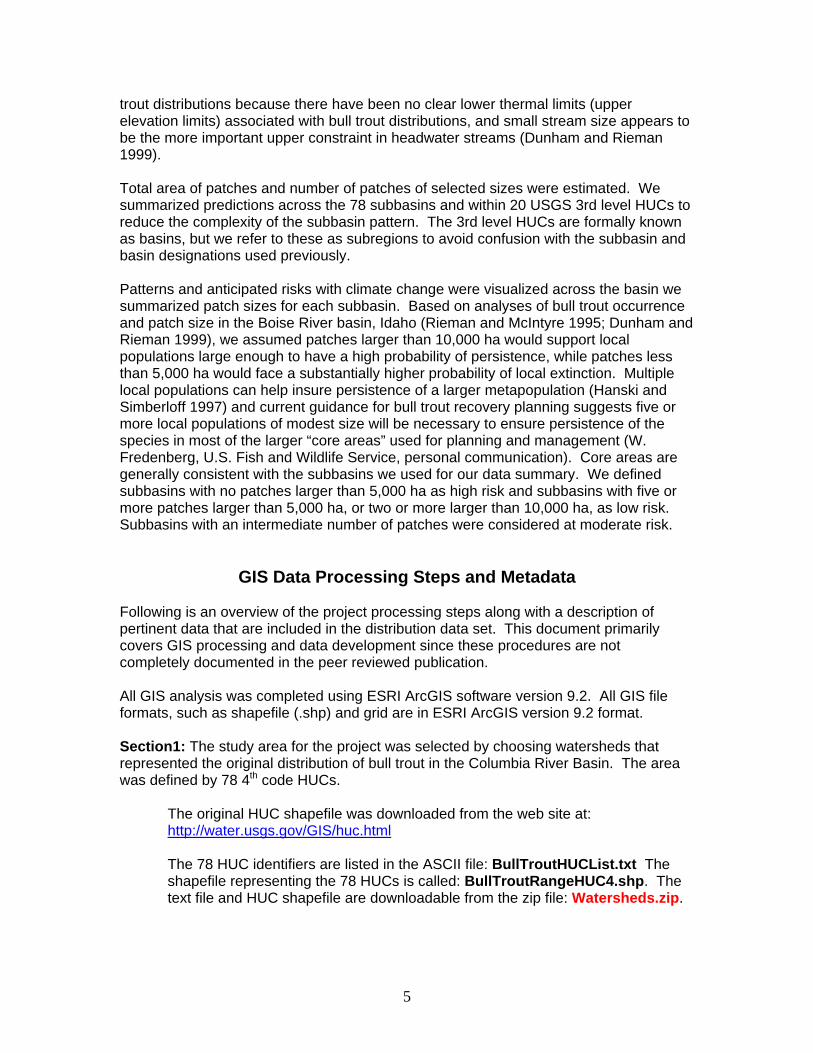
GIS Data Processing Steps and Metadata Following is an overview of the project processing steps along with a description of pertinent data that are included in the distribution data set. This document primarily covers GIS processing and data development since these procedures are not completely documented in the peer reviewed publication. All GIS analysis was completed using ESRI ArcGIS software version 9.2. All GIS file formats, such as shapefile (.shp) and grid are in ESRI ArcGIS version 9.2 format. Section1: The study area for the project was selected by choosing watersheds that represented the original distribution of bull trout in the Columbia River Basin. The area was defined by 78 4th code HUCs.

The original HUC shapefile was downloaded from the web site at: http://water.usgs.gov/GIS/huc.html

The 78 HUC identifiers are listed in the ASCII file: BullTroutHUCList.txt The shapefile representing the 78 HUCs is called: BullTroutRangeHUC4.shp. The text file and HUC shapefile are downloadable from the zip file: Watersheds.zip.

5

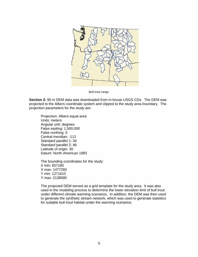
Bull trout range. Section 2: 90 m DEM data was downloaded from in-house USGS CDs. The DEM was projected to the Albers coordinate system and clipped to the study area boundary. The projection parameters for the study are:

Projection: Albers equal area Units: meters Angular unit: degrees False easting: 1,500,000 False northing: 0 Central meridian: -112 Standard parallel 1: 34 Standard parallel 2: 46 Latitude of origin: 30 Datum: North American 1983 The bounding coordinates for the study: X min: 657180 X max: 1477260 Y min: 1271610 Y max: 2138580 The projected DEM served as a grid template for the study area. It was also used in the modeling process to determine the lower elevation limit of bull trout under different climate warming scenarios. In addition, the DEM was then used to generate the synthetic stream network, which was used to generate statistics for suitable bull trout habitat under the warming scenarios.

6

90 m DEM (demcrb)

Section 3: A raster spatial model that depicts the current lower limit of bull trout within the Columbia basin was created. Not all of the grids used to create this initial lower limit model are included for distribution because of the large file size of each intermediate grid. The steps used to create the intermediate grids and the initial lower limit grid are described below.

We began with a grid template for the study area in the Albers projection with a cell size of 90 m. All cells in this grid had a value of 1. This grid was projected to the geographic coordinate system in units of decimal degrees (dd). The cell size was specified as 0.000834 dd, which is approximately 90 m. The file name for this grid was called constant1dd. Since the model for predicting the lower limit of bull trout contained variables for latitude and longitude, we next used the dd grid template to create two grids, one representing longitude and the other latitude. Each cell in the grids represents either the latitude or longitude of the study area. The raster layers were created using the GRID module in ArcInfo Workstation. Following are the expressions used to create these grids:

lat_dd = constant1dd * $$ymap lon_dd = constant1dd * $$xmap

Once the latitude and longitude grids were created they were reprojected back to the Albers coordinate system and named lat_alb and lon_alb.

7

Latitude grid (lat_alb)

Longitude grid (lon_alb)

Using these two grids, the lower limit model grid was created. The expression used in Spatial Analyst -> Map Algebra to create the model grid was:

8,693 – (190.8 * lat_alb) + (73.58 * lon_alb)

8

Lower limit model grid (low_limit)

Finally, the lower limit model grid and the 90 m DEM were combined to create the baseline lower limit of bull trout under current climate conditions. Following is the Map Algebra expression used to create this grid:

con(demcrb >= low_limit, 1, 0)

The result was clipped to the HUC boundaries representing the range of bull trout (clowlimbase).

Lower limit for bull trout under baseline (current) climate conditions (clowlimbase). Dark gray represents

thermally suitable habitat.

9

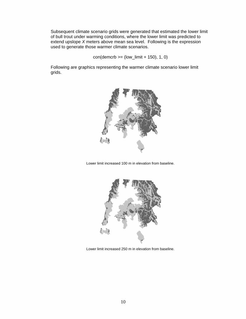
Subsequent climate scenario grids were generated that estimated the lower limit of bull trout under warming conditions, where the lower limit was predicted to extend upslope X meters above mean sea level. Following is the expression used to generate those warmer climate scenarios.

con(demcrb >= (low_limit + 150), 1, 0) Following are graphics representing the warmer climate scenario lower limit grids.

Lower limit increased 100 m in elevation from baseline.

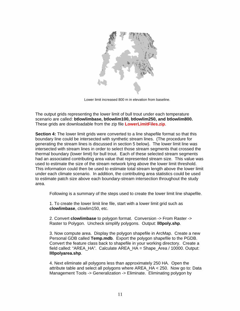
Lower limit increased 250 m in elevation from baseline.

10

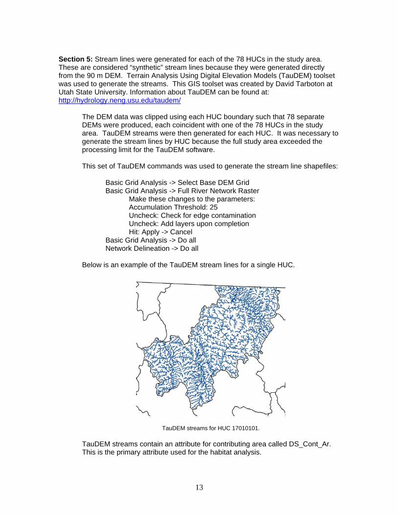
Lower limit increased 800 m in elevation from baseline.

The output grids representing the lower limit of bull trout under each temperature scenario are called: btlowlimbase, btlowlim100, btlowlim250, and btlowlim800. These grids are downloadable from the zip file LowerLimitFiles.zip. Section 4: The lower limit grids were converted to a line shapefile format so that this boundary line could be intersected with synthetic stream lines. (The procedure for generating the stream lines is discussed in section 5 below). The lower limit line was intersected with stream lines in order to select those stream segments that crossed the thermal boundary (lower limit) for bull trout. Each of these selected stream segments had an associated contributing area value that represented stream size. This value was used to estimate the size of the stream network lying above the lower limit threshold. This information could then be used to estimate total stream length above the lower limit under each climate scenario. In addition, the contributing area statistics could be used to estimate patch size above each boundary-stream intersection throughout the study area.

Following is a summary of the steps used to create the lower limit line shapefile. 1. To create the lower limit line file, start with a lower limit grid such as clowlimbase, clowlim150, etc. 2. Convert clowlimbase to polygon format. Conversion -> From Raster -> Raster to Polygon. Uncheck simplify polygons. Output: ll0poly.shp. 3. Now compute area. Display the polygon shapefile in ArcMap. Create a new Personal GDB called Temp.mdb. Export the polygon shapefile to the PGDB. Convert the feature class back to shapefile in your working directory. Create a field called: “AREA_HA”. Calculate AREA_HA = Shape_Area / 10000. Output: ll0polyarea.shp. 4. Next eliminate all polygons less than approximately 250 HA. Open the attribute table and select all polygons where AREA_HA < 250. Now go to: Data Management Tools -> Generalization -> Eliminate. Eliminating polygon by

11

border should be checked. Output: ll0elim.shp. You may need to do it twice. Output: ll0elim2.shp. 5. Now convert the eliminate file back to a grid. Conversion Tools -> To Raster -> Feature to Raster. The field should be GRIDCODE and cell size = 45. Be sure to set environments so that the output extent is the same as the lower limit raster and again the cell size is set to 45. Output: ll0grid45. 6. Run shrink on the grid. The number of cells should be 1. Zone value is also 1. Spatial Analyst Tools -> Generalization -> Shrink. Output: ll0shrink. 7. Convert the shrink grid back to polygon. Conversion -> From Raster -> Raster to Polygon. Uncheck simplify polygons. Output ll0shrinkpoly.shp. 8. Extract all polygons with value 1 and write to new shapefile. Do so by opening the attribute table and selecting all polygons with GRIDCODE = 1. Output: ll0shrinkonly1.shp. 9. Convert polygons to line format. Data Management Tools -> Features -> Feature to Line. Output: ll0shrinkline.shp. This is the line shapefile for the lower limit.

An example of the line shapefile for the baseline climate scenario is shown below:

Lower limit line shapefile representing baseline climate conditions.

The lower limit polyline shapefiles are called: LowerLimitLineBase.shp, LowerLimitLine100.shp, LowerLimitLine250.shp, and LowerLimitLine800.shp. These shapefiles are downloadable from the zip file LowerLimitFiles.zip.

12

Section 5: Stream lines were generated for each of the 78 HUCs in the study area. These are considered “synthetic” stream lines because they were generated directly from the 90 m DEM. Terrain Analysis Using Digital Elevation Models (TauDEM) toolset was used to generate the streams. This GIS toolset was created by David Tarboton at Utah State University. Information about TauDEM can be found at: http://hydrology.neng.usu.edu/taudem/

The DEM data was clipped using each HUC boundary such that 78 separate DEMs were produced, each coincident with one of the 78 HUCs in the study area. TauDEM streams were then generated for each HUC. It was necessary to generate the stream lines by HUC because the full study area exceeded the processing limit for the TauDEM software. This set of TauDEM commands was used to generate the stream line shapefiles:

Basic Grid Analysis -> Select Base DEM Grid Basic Grid Analysis -> Full River Network Raster

Make these changes to the parameters: Accumulation Threshold: 25 Uncheck: Check for edge contamination Uncheck: Add layers upon completion Hit: Apply -> Cancel

Basic Grid Analysis -> Do all Network Delineation -> Do all

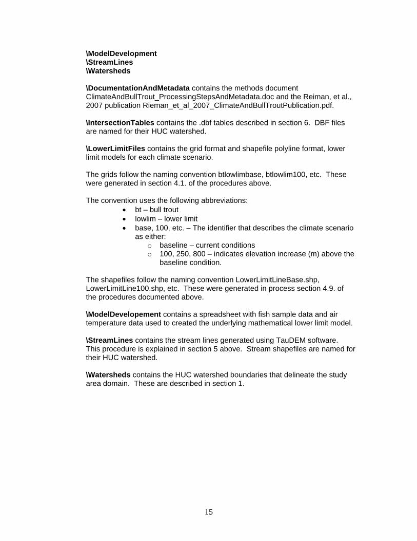
Below is an example of the TauDEM stream lines for a single HUC.

TauDEM streams for HUC 17010101.

TauDEM streams contain an attribute for contributing area called DS_Cont_Ar. This is the primary attribute used for the habitat analysis.

13

The TauDEM stream lines are available for each HUC from the downloadable zip file StreamLines.zip. 6) A Python script was created that intersected the lower limit line file (such as ll0shrinkline.shp) with the TauDEM stream layer (such as 17010101.shp). Analyses were completed on a HUC by HUC basis. The intersection records (where a stream line intersected a lower limit polyline) were selected and written to a .dbf file by the Python script. 78 tables (.dbf files) resulted from these analyses, for each temperature scenario (base, 100, 250 and 800). These tables were then input into SAS for further analysis as described in the publication.

Below is a portion of the attribute table from the .dbf files:

The field LINKNO is the unique identifier for each record and represents a single stream segment. DS_Cont_Ar is the contributing area at the downstream end of each stream segment. This attribute was used to estimate the size of the stream network within a patch, were the stream intersected the lower limit threshold line.

The intersection tables are available for each HUC from the downloadable zip file IntersectionTables.zip.

References Cited For a full citation of all of the references cited in this document, see the following paper, which is accessible on the Boise Lab, Stream Temperature Modeling web site: Rieman, B., D. Isaak, S. Adams, D. Horan, D. Nagel, C. Luce, D. Meyers., 2007. Anticipated Climate Warming Effects on Bull Trout Habitat and Populations Across the Interior Columbia River Basin .Transactions of the American Fisheries Society, 136:1552-1565.

The Distribution Data Set – Directory Structure and Naming Conventions

The directory structure for the distribution data set is described below. These folders will be created on the users computer when the downloadable zip files are uncompressed.

\DocumentationAndMetadata \IntersectionTables \LowerLimitFiles

14

15

\ModelDevelopment \StreamLines \Watersheds \DocumentationAndMetadata contains the methods document ClimateAndBullTrout_ProcessingStepsAndMetadata.doc and the Reiman, et al., 2007 publication Rieman_et_al_2007_ClimateAndBullTroutPublication.pdf. \IntersectionTables contains the .dbf tables described in section 6. DBF files are named for their HUC watershed.

\LowerLimitFiles contains the grid format and shapefile polyline format, lower limit models for each climate scenario. The grids follow the naming convention btlowlimbase, btlowlim100, etc. These were generated in section 4.1. of the procedures above. The convention uses the following abbreviations:

bt – bull trout lowlim – lower limit base, 100, etc. – The identifier that describes the climate scenario

as either: o baseline – current conditions o 100, 250, 800 – indicates elevation increase (m) above the

baseline condition. The shapefiles follow the naming convention LowerLimitLineBase.shp, LowerLimitLine100.shp, etc. These were generated in process section 4.9. of the procedures documented above.

\ModelDevelopement contains a spreadsheet with fish sample data and air temperature data used to created the underlying mathematical lower limit model.

\StreamLines contains the stream lines generated using TauDEM software. This procedure is explained in section 5 above. Stream shapefiles are named for their HUC watershed.

\Watersheds contains the HUC watershed boundaries that delineate the study area domain. These are described in section 1.