model for shear ﬂow

arX

iv:1

107.

0580

v1 [

phys

ics.

flu-

dyn]

4 J

ul 2

011

Turbulent transition in a truncated 1D

model for shear flow

By J. H. P. Dawes and W. J. Giles

Department of Mathematical Sciences, University of Bath, Claverton Down, BathBA2 7AY, UK

We present a reduced model for the transition to turbulence in shear flow that issimple enough to admit a thorough numerical investigation while allowing spatio-temporal dynamics that are substantially more complex than those allowed in pre-vious modal truncations.

Our model allows a comparison of the dynamics resulting from initial perturba-tions that are localised in the spanwise direction with those resulting from sinusoidalperturbations. For spanwise-localised initial conditions the subcritical transition toa ‘turbulent’ state (i) takes place more abruptly, with a boundary between laminarand ‘turbulent’ flow that is appears to be much less ‘structured’ and (ii) results ina spatiotemporally chaotic regime within which the lifetimes of spatiotemporallycomplicated transients are longer, and are even more sensitive to initial conditions.

The minimum initial energy E0 required for a spanwise-localised initial pertur-bation to excite a chaotic transient has a power-law scaling with Reynolds numberE0 ∼ Rep with p ≈ −4.3. The exponent p depends only weakly on the width ofthe localised perturbation and is lower than that commonly observed in previouslow-dimensional models where typically p ≈ −2.

The distributions of lifetimes of chaotic transients at fixed Reynolds number arefound to be consistent with exponential distributions.

Keywords: fluid flow; turbulence; dynamical systems

1. Introduction

The transition from laminar to turbulent states has been a central problem in fluidmechanics for many decades. Since the 1960s, promising lines of attack have beenopened up through the use of ideas from dynamical systems theory coupled to thethorough investigation of reduced versions of the Navier–Stokes equations. Per-haps the best-known example of such a reduction is the derivation of the Lorenzequations as a model of the onset of thermal convection in a layer of fluid heatedfrom below (Lorenz 1963). Although the set of three nonlinear ODEs that comprisethe Lorenz 1963 model displays a wealth of interesting dynamical behaviour, littleof this is relevant to the original fluid-mechanical problem. However, similar ap-proaches yield convincing agreement over wide ranges of parameter values in otherfluid-mechanical situations, for example thermal convection in the presence of amagnetic field, and the onset of Taylor vortices in the flow between rotating coax-ial concentric cylinders. In situations such as these the flow undergoes a series ofbifurcations before becoming chaotic, in a sense that can be given a clear meaningin terms of the behaviour of the reduced model comprising nonlinear ODEs.

Article submitted to Royal Society TEX Paper

http://arxiv.org/abs/1107.0580v1

2 J. H. P. Dawes and W. J. Giles

In contrast, the transition to turbulence in shear flows appears not to proceedthrough a sequence of bifurcations, but to be linked to the appearance, at a criticalReynolds number Rec, of a chaotic saddle in phase space: a complicated collection ofunstable equilibria and time-periodic orbits which results in ever longer transientsbefore the flow relaxes to a purely laminar state. For a review, and substantialnumbers of references to the literature (although with an emphasis on pipe flow),see Kerswell (2005). The significance of Rec is that for Re < Rec the laminarstate is a global attractor and trajectories appear to evolve rapidly towards it,while for Re > Rec other (usually unstable) invariant sets exist in phase space.These new invariant sets cause increasingly long transient excursions to take placebefore relaminarisation occurs, for initial conditions that are sufficiently far fromthe laminar profile. Small perturbations to the laminar state still decay rapidlytowards it, and there appears to be a distinct boundary separating the behaviourof trajectories into those that relax rapidly and those which undergo long transientexcursions. This laminar-turbulent boundary is sometimes referred to as the ‘edge ofchaos’. Despite these differences in phenomenology and dynamics, reduced modelsconstructed along the same lines as the Lorenz model have provided substantialinsight into both the physical origin of this transition to self-sustaining complicatedmotion, and the mathematical organisation of equilibria and periodic orbits insidethe chaotic saddle.

The study by Waleffe (1997) provides the direct inspiration for the present work.Waleffe showed that a low-order reduced model could be constructed that elucidatedthe different elements of a self-sustaining process (SSP) that allowed sufficientlylarge deviations from the laminar flow profile to persist indefinitely. The SSP can bebriefly described as follows. Weak streamwise vortices (i.e. vortical rolls whose axesare aligned with the primary flow direction) distort the streamwise velocity profileby moving high and low-speed fluid around. This distortion generates streamwisestreaks of fluid that are moving faster and slower than the fluid around them. Thestreaks are unstable to modes which create vortical eddies oriented in the wall-normal direction, orthogonal to the streamwise vortices, and the resulting three-dimensional re-organisation of the flow reinforces the streamwise vortices.

Waleffe’s model simplified the Navier–Stokes equations first by considering, notplane Couette flow between rigid boundaries, but a modified problem in which theboundaries are stress-free and the laminar profile is sinusoidal, sustained by anartificially-applied pressure term. It appears that the physics of the SSP is ratherinsensitive to these modifications. The second set of simplifications concern theGalerkin expansion of the velocity field in all three directions: streamwise (x), wallnormal (y) and spanwise (z). Thus Waleffe considered a model comprising 8 of thelowest-wavenumber Fourier modes in this Galerkin expansion. These 8 modes werechosen in order to capture the central elements of the SSP, and to be self-consistentin the sense that the nonlinear (quadratic) interactions between these 8 modespreserve energy just as the full advective nonlinearity in the Navier–Stokes equa-tions does. Having projected out the spatial dependence of the dynamics onto thesemodes, the problem reduces to a far simpler set of ordinary differential equations(ODEs) for the time-dependent mode amplitudes. Subsequent work, in particularby Eckhardt & Mersmann (1999) and Moehlis, Faisst and Eckhardt (2004, 2005)extended Waleffe’s model to include an additional physical insight: that the basiclaminar profile of the shear flow will itself be modified by the nonlinear interac-

Article submitted to Royal Society

Transition in a 1D shear flow model 3

tions with streamwise vortices and streaks. Moehlis et al developed a 9-mode ODEmodel that was amenable to investigation in substantial detail. In particular theydiscussed the lifetimes of perturbations as the Reynolds number increased, locatingthe onset of complicated dynamics, and they also discussed the probabilistic distri-bution of lifetimes at fixed Reynolds number from randomised initial conditions ofequal energy.

It is clear that the assumptions made by these authors concerning spatial period-icity seems much easier to argue for in the streamwise and wall-normal directionsthan in the spanwise direction; indeed recent work by Schneider and co-workers(Schneider et al 2009; 2010a; 2010b) (see also Duguet, Schlatter and Henningson,2009) has concentrated on understanding the formation of structures which arespatially localized in z: very far from periodic in this direction.

With this in mind we propose in this paper an extension of Waleffe’s modelwhich is a reduction of the Navier–Stokes equations to a collection of PDEs in zand t: we adopt the Fourier mode truncations that Waleffe used in order to removethe dependence on the streamwise x and wall-normal y coordinates since numericalwork shows that, at least for some of these equilibrium and periodic orbit states,the flow structure in these coordinates can be well-approximated by a small numberof Fourier modes.

By retaining full dependence on the spanwise coordinate z we admit both thespatially-periodic solutions of Waleffe and the formation of localized states. In addi-tion, a wealth of spatio-temporal complexity is allowed. Our study is very similar inspirit to work by Manneville and co-authors (Manneville & Locher 2000; Manneville2004; Lagha & Manneville 2007) who preserve full resolution in two directions(streamwise and spanwise) and use Galerkin truncation only in the third (‘wall-normal’) direction. This enables these authors to consider the dynamics aroundturbulent spots that are localised in both the streamwise and spanwise directions,at the cost of more intensive numerical computations. Their work is therefore com-plementary to that presented here. We remark also that reduced models, of differentkinds, have been used both in pipe flow (Willis & Kerswell 2009) and in under-standing the formation of turbulent-laminar bands in plane Couette flow (Barkley& Tuckerman 2007).

The structure of the paper is as follows. In section 2 we discuss the derivationof our PDE extension of Waleffe’s ODE model. In section 3 we present the resultsof our numerical investigations into the transition to turbulence described by themodel. We conclude in section 4.

2. Derivation of the PDE model

In this section we define sinusoidal shear flow and summarise the Galerkin trunca-tion that we use to derive our simplified model for turbulent transition.

Following Waleffe (1997) and Moehlis et al (2004), we use the usual Carte-sian coordinate conventions that x is the downstream direction (‘streamwise’), y isthe direction of the shear gradient, i.e. normal to the sidewalls and z is the span-wise direction. We write the Navier–Stokes equations for incompressible flow in thenondimensionalised form

∂u

∂t+ u · ∇u = −∇p+ F(y) +

1

Re∇2

u, (2.1)



where we have scaled lengths by h/2 where h is the width of the channel, velocitiesby U0 the velocity of the laminar profile at a distance h/4 from the upper boundaryand pressure by U2

0 ρ where ρ is the density of the fluid. The Reynolds numberRe is therefore given by Re = U0h/(2ν), ν being the kinematic viscosity. Theevolution of (2.1) is subject to the usual incompressibility condition ∇ · u = 0 andthe conditions for impermeable and stress-free upper and lower boundaries

uy = 0, and∂ux

∂y=

∂uz

∂y= 0 at y = ±1. (2.2)

The flow is assumed to be periodic in the x and z directions, with periodicities Lx

and Lz respectively. We take the body force term F(y) to be

F(y) =

√2β2

Resinβy ex, (2.3)

where ex is the unit vector in x direction and it is convenient to define the constantβ = π/2. The laminar profile is then the steady solution

u =√2 sinβyex, (2.4)

of (2.1) - (2.3), as shown in figure 1. We note that although the ‘sinusoidal shear

x

z

y

Figure 1. Geometry of the domain, illustrating the basic sinusoidal shear profileu =

√2 sin βyex which is sustained by the applied body force term.

flow’ profile (2.4) has an inflection point, the flow is linearly stable for all Re (Drazin& Reid 1981).

We now turn to our solution ansatz. We write the velocity field in the form

u = uM +∇×ΦT +∇×∇×ΦP , (2.5)

where the subscripts denote mean, toroidal and poloidal components which are,respectively, expressed as sums of the first few Fourier modes in each case:

uM = (A1 sinβy +A2) ex,

ΦT = A3 cosβy ex

+(A4 sinαx −A5 cosαx sin βy −A6 cosαx +A7 sinαx sinβy) ey,

ΦP = A8 cosαx cos βy ey.



Table 1. Comparison of notation.

This paper A1 A2 A3 A4 A5 A6 A7 A8

Waleffe (1997) M U V A C B D E

const cos γz sin γz const const cos γz cos γz sin γz

We define the streamwise and spanwise wavenumbers α = 2π/Lx and γ = 2π/Lz fornotational convenience. The amplitudes A1, . . . , A8 are functions of z and t whoseevolution can be obtained by substituting (2.5) into (2.1). Note that the form ofthe ansatz implies that incompressibility and the boundary conditions (2.2) areautomatically satisfied.

The amplitudes A1, . . . , A8 correspond exactly, in terms of their Fourier depen-dence in x and y, to the modes selected by Waleffe (1997). For reference, table 1summarises the correspondence.

We now briefly describe the role that each mode plays in the dynamics. A1 is theamplitude of the sinusoidal shear profile; the laminar state corresponds to A1 =

√2,

A2 = · · · = A8 = 0. A2 describes variations in z of the streamwise velocity, i.e.the formation of streamwise streaks. A3 describes the formation of x-independentstreamwise vortices that redistribute the shear profile. Modes A4, . . . , A7 describe,as in Waleffe (1997) the development of x-dependent distortions of the streaks,and in particular the linear instability of the x-independent streaks described byA2. These modes have no velocity component in the vertical (i.e. y) direction. A8

describes ‘oblique rolls’ and, in contrast to modes A4, . . . , A7, has a non-zero verticalvelocity component but no vertical vorticity component.

To derive evolution equations for the modes A1, . . . , A8 we use Fourier orthogo-nality in the x and y directions combined with projections onto individual compo-nents of either the velocity field u, the vorticity field ω = ∇×u or (for A8) the curlof the vorticity field. For later convenience we introduce the differential operatorsD2

α, D2

β and D2

αβ which correspond to the action of −∇2 on different Fourier modes:

D2

α ≡ α2 − ∂zz, D2

β ≡ β2 − ∂zz, D2

αβ ≡ α2 + β2 − ∂zz.

We denote ∂Aj/∂z by A′j for j = 1, . . . , 8. Considering first the ex component of u

in (2.1) we obtain the following PDEs in z and t for A1 and A2:(

∂t +1

ReD2

β

)

A1 = −βA′

2A3 +α

2(A′′

4A5 −A4A′′

5) +α

2(A6A

′′

7 −A′′

6A7)

+β

2(A′′

6A′

8 − α2A6A′

8) +

√2β2

Re, (2.6)

(

∂t −1

Re∂zz

)

A2 = −β

2(A1A3)

′ +α

2(A′′

4A6 −A4A′′

6 )−α

4(A′′

5A7 −A5A′′

7)

−α2β

4(A5A8)

′ +β

4(A′

5A′

8)′, (2.7)

Now we turn to the vorticity ω. For A3, A4 and A6 we find that only one componentof ω contains a contribution from each of these; taking the curl of (2.5) the termsinvolving A3, A4 and A6 are

ω = D2

βA3 cosβy ex +(

D2

αA4 sinαx−D2

αA6 cosαx)

ey.



Therefore it is straightforward to consider the x and y components of the vorticityequation obtained by applying the operators ex · ∇× and ey · ∇× to (2.1) in orderto obtain evolution equations for A3, A4 and A6:

(

∂t +1

ReD2

β

)

D2

βA3 = −α2β(A4A7)′ − α2β(A5A6)

′ +α3

2(A4A8)

′′

−α

2(A4A

′′

8)′′ + αβ2A′

4A′

8 +α3β2

2A4A8

+αβ2

2A4A

′′

8 , (2.8)

(

∂t +1

ReD2

α

)

D2

αA4 =α

2(A1A

′′

5 −A′′

1A5)−α3

2A1A5 + α(A2A

′′

6 −A′′

2A6)

−α3A2A6 +β

2(A3A

′

7)′′ − α2β

2A3A

′

7 − α2βA′

3A7

−α3β2

2A3A8 +

αβ2

2(A3A

′′

8 −A′′

3A8), (2.9)

(

∂t +1

ReD2

α

)

D2

αA6 =α3

2A1A7 −

α

2(A1A

′′

7 −A′′

1A7) + α2βA′

1A8

+α2β

2A1A

′

8 −β

2(A1A

′

8)′′ + α3A2A4

−α(A2A′′

4 −A′′

2A4) +β

2(A3A

′

5)′′ − α2βA′

3A5

−α2β

2A3A

′

5, (2.10)

Evolution equations for A5, A7 and A8 are derived similarly, using (for A5 andA7) the projection operator ey ·∇× and (for A8) the projection operator ey ·∇×∇×applied to (2.1). The resulting evolution equations are

(

∂t +1

ReD2

αβ

)

D2

αA5 = α3A1A4 − α(A1A′′

4 −A′′

1A4) + α3A2A7

−α(A2A′′

7 −A′′

2A7)− β(A′

2A′

8)′

+α2βA′

2A8 − α2β(A3A6)′ + β(A3A

′′

6 )′, (2.11)

(

∂t +1

ReD2

αβ

)

D2

αA7 = −α3A1A6 + α(A1A′′

6 −A′′

1A6)− α3A2A5

+α(A2A′′

5 −A′′

2A5) + β(A3A′′

4)′

−α2β(A3A4)′, (2.12)

(

∂t +1

ReD2

αβ

)

D2

αβD2

αA8 = −2α2β(A′

1A6 +A′

2A5)− 2αβ2A′

3A′

4

+α(A′′

3A4)′′ − α(α2 + β2)A′′

3A4. (2.13)

Equations (2.6) - (2.13) are a closed set of nonlinear PDEs in z and t which form atruncated model of the dynamics of sinusoidal shear flow. Crucially these equations



satisfy two consistency checks: the nonlinear terms in (2.6) - (2.13) conserve energyand so reflect the conservative nature of the full u·∇u nonlinearity in (2.1). Secondlythis model reduces to the model of Waleffe (1997) in the special case in which theamplitudes A1, . . . , A8 are taken to be periodic in the z-direction, after applyingappropriate projection onto orthogonal Fourier modes in z. We discuss each of theseimportant issues in more detail in the following subsections.

(a) Nonlinear terms and energy conservation

In this subsection we show that the nonlinear terms in (2.6) - (2.13) do notcontribute to the energy budget for the dynamics. This is a physically crucial prop-erty in constructing any reasonable reduced model for shear flows: the only energysource term must be the body force F(y) that drives the laminar flow, and the onlysource of dissipation must be (linear) viscous diffusion.

We define the (dimensionless) total kinetic energy of the flow to be

E =1

2

∫

Ω

u · u dx dy dz, (2.14)

where Ω = [0, π/α]× [−1, 1]× [0, Lz] is (one half of) the domain (in x, y, z coordi-nates) occupied by the fluid. We substitute our ansatz (2.5) into (2.14) and carryout the x and y integrals, noting that Fourier orthogonality enables us to removeall cross-terms except those involving A7 and A8 since they have the same Fourierdependencies; their contributions to u are

u7 =

−A′7 sinαx sin βy

0

αA7 cosαx sin βy

, and u8 =

−αβA8 sinαx sin βy

(α2A8 −A′′8) cosαx cosβy

−βA′8 cosαx sin βy

.

Hence the kinetic energy E is given by

E =π

2α

∫ Lz

0

A2

1 + 2A2

2 + (A′

3)2 + β2A2

3 + (A′

4)2 + α2A2

4

+1

2(A′

5)2 +

α2

2A2

5 + (A′

6)2 + α2A2

6 +1

2(αβA8 −A′

7)2

+1

2

(

α2A8 −A′′

8

)2+

1

2(αA7 − βA′

8)2dz,

≡ π

2α

∫ Lz

0

E(z, t) dz, (2.15)

which defines the ‘local’ energy quantity E(z, t). After integrating several terms byparts, and noting that the boundary contributions vanish (since we use a periodicboundary condition in z), and also after some manipulation of the cross-termsinvolving A7 and A8, we obtain the expression

E =π

2α

∫ Lz

0

A2

1 + 2A2

2 +A3D2

βA3 +A4D2

αA4 +1

2A5D2

αA5

+A6D2

αA6 +1

2A7D2

αA7 +1

2A8D2

αβD2

αA8 dz.



We can now compute the time evolution of the kinetic energy by differentiatingwith respect to time. After carrying out further integrations by parts we find

dE

dt=

π

2α

∫ Lz

0

2A1A1 + 4A2A2 + 2A3D2

βA3 + 2A4D2

αA4

+A5D2

αA5 + 2A6D2

αA6 +A7D2

αA7 +A8D2

αβD2

αA8 dz. (2.16)

We now substitute for the time derivatives using the PDEs (2.6) - (2.13). Theinterest in pursuing this calculation is that at this stage we find that the conservativenature of the quadratic nonlinearities in (2.6) - (2.13) becomes apparent since allthe cubic terms cancel (after appropriate integrations by parts). We are then leftwith a single linear source term and a collection of quadratic dissipation terms:

dE

dt=

πβ2√2

αRe

∫ Lz

0

A1 dz −π

2αRe

∫ Lz

0

2(

β2A2

1 + (A′

1)2)

+ 4(A′

2)2

+2(D2

βA3)2 + 2(D2

αA4)2 + (D2

αA5)2 + β2

(

α2A2

5 + (A′

5)2)

+2(D2

αA6)2 + (D2

αA7)2 + β2

(

α2A2

7 + (A′

7)2)

+α2(D2

αβA8)2 + (D2

αβA′

8)2 dz.

The derivative of this equation for the evolution of the total kinetic energy, whichdescribes the balance between the driving provided by the body force term F(y) andviscous dissipation, makes it clear that the nonlinear terms in (2.6) - (2.13) conserveenergy. This justifies the self-consistency of the selection of just the eight modesA1, . . . , A8 in the reduced model: by including exactly these modes, no unphysicaleffects are introduced into the energy evolution.

(b) Relation with the model of Waleffe (1997)

Waleffe (1997) considered a far simpler modal truncation in which each modecontains only a single Fourier mode in z. This introduces an additional parameter:the wavenumber γ in the z-direction, but the model comprises ODEs rather thanPDEs for the eight amplitudes and is therefore much more amenable to analysis.The derivation of such a modal truncation is slightly simpler than that describedabove since one can use Fourier orthogonality directly in the z-direction as wellas in x and y. In fact, the reduced model (2.6) - (2.13) reduces exactly (afterrescalings of the amplitude variables) to that discussed by Waleffe if one inserts thecorresponding trigonometric dependencies and then projects out unwanted modesthat arise from some of the nonlinear terms. This projection step is self-consistent inthe sense that in both (2.6) - (2.13) and the ODEs derived by Waleffe the nonlinearterms conserve energy. Table 1 lists the Fourier dependence in the z-direction thatWaleffe (1997) assumed for each mode.

Waleffe observed that his ODE model had a number of deficiencies, for examplethe streaks (described by A2) were unstable to x-dependent perturbations, witheven and odd symmetry in y, only if the wavenumber γ was sufficiently large:γ2 > α2 and γ2 > α2 + β2, respectively, to be precise.

More seriously, he discusses the inadequacy of his ODE model in capturing theinteraction between the mean shear (M , or equivalently A1) and the x-dependentmodes (A, C, B and D, or equivalently A4, . . . , A7) that arise from consideration



of advection by the mean shear. We observe that in (2.6) - (2.13) these quadraticinteractions take far more complex forms that in many cases vanish identically whenthe simple Fourier mode dependencies in z that are listed in table 1 are imposed.In particular the mean shear A1 is influenced by new combinations of x-dependentmodes which do not arise in the ODE model because the expressions A6A

′′7 −A′′

6A7

andA′′4A5−A4A

′′5 which are present in (2.6) vanish identically in the ODE reduction.

Terms with a structure identical to this (i.e. of the form AnA′′m − A′′

nAm) appearin several of the the other amplitude equations. Compared with Waleffe’s ODEmodel, the other qualitatively new couplings introduced in (2.6) - (2.13) are theterm β(A3A

′′6 )

′ in (2.11) and the term −2α2βA′1A6 in (2.13).

3. Numerical results

In this section we present the results of time-stepping the system of PDEs (2.6) -(2.13) over the range 50 ≤ Re ≤ 200. Our numerical method is the pseudospectralexponential time-stepping scheme referred to as ‘ETD2’ by Cox & Matthews (2002),using 128 Fourier modes in z, and suitably small timesteps such that our resultswere insensitive to the timestep used.

As in Moehlis et al (2004) our primary interest is in the emergence of a chaoticsaddle in phase space. This is indicated by the lifetimes of chaotic transients astrajectories evolve towards the linearly stable laminar state, having started frominitial conditions that are far from the laminar equilibrium.

(a) Initial conditions and domain parameters

The lifetimes of chaotic transients are of course sensitive to the choice of initialcondition, and in order to investigate the response of the flow to a spatially localisedperturbation we took initial conditions corresponding to a Gaussian profile, scaledso that the four modes A3, A4, A5 and A6 gave equal contributions to the initialkinetic energy E0. Later, in subsection 3(f), we compare these results with thoseobtained using a sinusoidal initial condition.

Specifically our Gaussian initial condition takes the form A1 = A2 = A7 = A8 =0 and

Aj = cj exp

(

− (z − Lz/2)2

2σ2

)

, (3.1)

for j = 3, . . . , 6, where the coefficient σ describes the width of the Gaussian, andthe normalisation constants cj are given by

c3 =

√

E0σα

2π√π(

β2σ2 + 1

2

) , (3.2)

c4 = c6 =

√

E0σα

2π√π(

α2σ2 + 1

2

) , (3.3)

c5 =

√

E0σα

π√π(

α2σ2 + 1

2

) . (3.4)



The differencies in the expressions for c3, . . . , c6 reflect the different contributionsmade by A3, . . . , A6 to the kinetic energy (2.15).

We present results for a domain size Lx = 1.75π, Lz = 1.2π corresponding tothe ‘minimal flow unit’ identified by previous authors (Hamilton, Kim & Waleffe,1995, and adopted by Moehlis et al 2004) as the smallest domain in which sustainedspatiotemporally chaotic dynamics have been found numerically. We consider valuesfor σ in the range 0.2 ≤ σ ≤ 0.8, initially setting σ = 0.2, so that the initial Gaussiandisturbance is always spatially well-localised in the z direction.

(b) Results at fixed Reynolds numbers

Our numerical integrations are carried out until either the dynamics approachesvery close to the laminar state, or until 1000 dimensionless time units of h/(2U0)have elapsed: this is the maximum lifetime that transients are followed for in ourcomputations. We follow transients for the range 50 ≤ Re ≤ 200, increasing Re insteps of unity, and increasing initial kinetic energy E0 in the range 0 < E0 < 3.0 insteps of 0.01.

At low Reynolds numbers, Re < 117, we find numerically that all initial condi-tions decay monotonically towards the stable laminar equilibrium, with a lifetimethat increases slowly with E0 in the range 0 < E0 < 1.7 approximately, and then de-creases slowly as E0 increases further. For Re ≥ 117 the dynamics changes abruptlyand initial energies around E0 = 1.7 show far longer transients, as indicated in fig-ure 2 which shows the lifetimes of trajectories for four fixed values of Re, as E0

varies. The overall impression of figure 2 is of a well defined transition from laminarto spatio-temporally complex dynamics for a range of initial perturbations. It isclear that windows of rapid attraction to the laminar state remain, for example forRe = 143 and initial energies around E0 = 1.3.

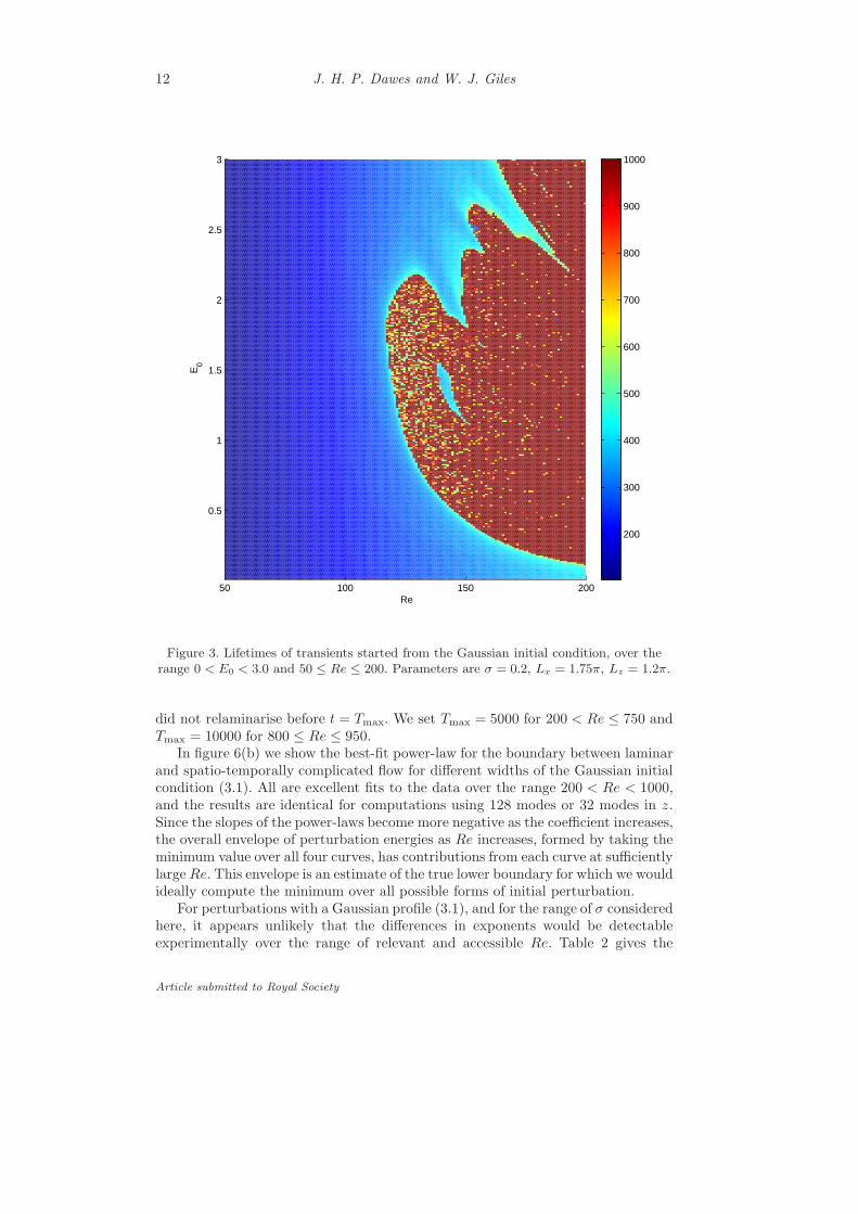
(c) Transition boundary and structure of the chaotic saddle

The well defined ‘transition boundary’ at which there is an abrupt increase inlifetimes is shown clearly in figure 3 which presents a colour-coded surface plotof lifetimes as Re and E0 vary. In contrast to previous similar plots, for examplefigure 6 of Moehlis et al. (2004), and see also figure 11 in the present paper, wherespatio-temporally complicated transients appear at around Re = 120 at the endsof ‘wispy’ dendritic fingers that coalesce as Re increases, figure 3 indicates thesudden appearance of a ‘fatter’ chaotic saddle in phase space. The chaotic saddleappears to become less ‘porous’ as Re increases, and there appears to be only onesubstantial hole, at around Re = 140, E0 = 1.4. As in Moehlis et al. (2004) wemight anticipate that figure 3 has fine scale structure as we zoom in. In contrast tothe results of that paper we find however that finer-scale investigations do not revealany coherent organisation to the lifetimes: instead of regions of concentric bandsof different colours, for example, we find merely fine-scale apparent randomnessand intermittency. This is illustrated in figure 4. Figure 4(a) shows the region130 ≤ Re ≤ 140, 1.6 ≤ E0 ≤ 1.7 with a ten-fold increase in the resolution alongeach axis. Figure 4(b) shows a further order of magnitude increase in the resolutionboth in Re and in E0; this part of the figure corresponds to the region withinthe black box in the centre of figure 4(a). This very detailed enlargement appears



0 0.5 1 1.5 2 2.5 3200

300

400

500

600

700

800

900

1000

E0

Life

time

143128

117

108

Figure 2. (Online version in colour.) Lifetimes of transients started from the Gaussianinitial condition, for initial kinetic energies 0 < E0 < 3.0 for Re = 108 (black, +),Re = 117 (red, ), Re = 128 (blue, ♦) and Re = 143 (magenta, ). Parameters areσ = 0.2, Lx = 1.75π, Lz = 1.2π.

to exhibit some slight correlation, for example a propensity to favour lifetimes ofaround 600 time units at Re ≈ 135.4 but otherwise the unpredictable intermittentnature of the dynamics continues as we consider finer and finer divisions in Reand E0. This qualitative observation should be contrasted with the lifetimes figuresplotted by Moehlis et al. (2004) which exhibit much more structure. We return tothis point in section 3(f).

The lower boundary of the chaotic saddle is of particular physical interest, sinceit describes the smallest amplitude perturbation required to produce an extendedchaotic transient. For the particular form of perturbation used here, in the caseσ = 0.2, we find numerically that the lower boundary in figure 3 is remarkably wellfitted by a power law curve as illustrated in the log-log plot in figure 5. Additionalcomputations show that a power law continues to provide a very good fit as Reis increased, up to at least Re = 103, as shown in figure 6(a). The black curve infigure 6(a) is the best-fit curve

E0 =

(

122

Re

)4.6

. (3.5)

Blue squares in figure 6 indicate that the flow returned to laminar before the com-putational time limit Tmax was reached, while red + signs indicate that the flow



50 100 150 200

0.5

1

1.5

2

2.5

3

Re

E0

200

300

400

500

600

700

800

900

1000

Figure 3. Lifetimes of transients started from the Gaussian initial condition, over therange 0 < E0 < 3.0 and 50 ≤ Re ≤ 200. Parameters are σ = 0.2, Lx = 1.75π, Lz = 1.2π.

did not relaminarise before t = Tmax. We set Tmax = 5000 for 200 < Re ≤ 750 andTmax = 10000 for 800 ≤ Re ≤ 950.

In figure 6(b) we show the best-fit power-law for the boundary between laminarand spatio-temporally complicated flow for different widths of the Gaussian initialcondition (3.1). All are excellent fits to the data over the range 200 < Re < 1000,and the results are identical for computations using 128 modes or 32 modes in z.Since the slopes of the power-laws become more negative as the coefficient increases,the overall envelope of perturbation energies as Re increases, formed by taking theminimum value over all four curves, has contributions from each curve at sufficientlylargeRe. This envelope is an estimate of the true lower boundary for which we wouldideally compute the minimum over all possible forms of initial perturbation.

For perturbations with a Gaussian profile (3.1), and for the range of σ consideredhere, it appears unlikely that the differences in exponents would be detectableexperimentally over the range of relevant and accessible Re. Table 2 gives the



130 132 134 136 138 140

1.61

1.62

1.63

1.64

1.65

1.66

1.67

1.68

1.69

1.7

Re

E0

0

100

200

300

400

500

600

700

800

900

1000

135 135.2 135.4 135.6 135.8 136

1.651

1.652

1.653

1.654

1.655

1.656

1.657

1.658

1.659

1.66

Re

E0

0

100

200

300

400

500

600

700

800

900

1000

(a) (b)

Figure 4. (Online version in colour.) Enlargements of figure 3 showing a lack of coherentorganisation to the lifetimes at higher resolution in Re and E0. (a) Transient lifetimesover the range 1.6 < E0 < 1.7 and 130 ≤ Re ≤ 140. (b) Transient lifetimes over the range1.65 < E0 < 1.66 and 135 ≤ Re ≤ 136 as indicated by the black square in (a). For bothfigures, the other parameter values are σ = 0.2, Lx = 1.75π, Lz = 1.2π.

details of the best-fit parameters of the power-laws shown in figure 6(b), using afunctional form E0 = (c/Re)p.

(d) Lifetime distributions

Moehlis et al also computed the distribution of lifetimes of turbulent transientsat fixed initial energies and Reynolds numbers. They found that the survival proba-bility P (T ) that the solution had not decayed back to the laminar state after a timeT was distributed exponentially, with a mean lifetime that increased rapidly withRe above the critical value at which the chaotic saddle appeared. Numerically, weconstruct a lifetime distribution by distributing the initial energy randomly acrossa subset of the modes. For our spatially-extended model there are two possibleapproaches to randomising the distribution of energy.

In the first approach, the total initial energy is distributed uniformly on a spher-ical energy shell. This can be achieved straightforwardly by modifying the expres-sions (3.2) - (3.4) for the normalisation coefficients by replacing E0 with 4E0ξ

2j in

the expression for coefficient cj, where j = 3, . . . , 6. The coordinates ξj are those of

points distributed at random over the unit sphere in R4 given by

∑6

j=3ξ2j = 1. We

refer to this as randomising over the amplitudes of the perturbations.In the second approach, the central position of each Gaussian perturbation Aj

is shifted randomly in z away from the centre of the domain Lz/2, i.e. the values ofthe coefficients c3, . . . , c6 are left unchanged but the centre of the Gaussian in (3.1)is modified for each amplitude Aj . Since we employ periodic boundary conditions,the total energy in the perturbation is preserved. We refer to this procedure asrandomising over the locations of the perturbations. Figure 7 shows the results ofthe first approach at two Reynolds numbers quite close to the transition boundary.At low lifetimes (T < 200) the survival probability remains unity since any transienttakes at least this finite amount of time to decay to within the prescribed thresholdof the laminar state. As T increases there is an initial sharp drop indicating that asubstantial proportion of trajectories do decay rapidly, with lifetimes in the range



102

102.1

102.2

102.3

10−1

100

Re

E0

200

300

400

500

600

700

800

900

1000

Figure 5. Log–log plot of transient lifetimes over the range 0.1 < E < 3.0 and100 ≤ Re ≤ 200 to show power law form of the lower boundary of the attractor. Thesolid (red) line indicates the power-law E0 =

(

125

Re

)4.65. Parameter values are σ = 0.2,

Lx = 1.75π, Lz = 1.2π.

200 < T < 400. At larger T the distribution becomes close to a straight line onthe linear-log plot, which is consistent with an exponential distribution P (T ) ∼a1 exp(−a2T ) for T ≥ 400 (approximately), as indicated by the dashed line. ForRe = 130 the best-fit coefficient values are a1 = 3.93× 10−1 and a2 = 8.65× 10−4.For Re = 140 the best-fit coefficient values are a1 = 4.57 × 10−1, a2 = 5.11 ×10−4. Similarly, figure 8 shows the lifetime distribution computed from the secondapproach, randomising over the locations of the perturbations. The distributionshows very similar characteristics to that in figure 7(a) and is again well-describedby an exponential distribution with best-fit parameters a1 = 4.24× 10−1 and a2 =8.32 × 10−4. We observe that the values for the coefficient a2 are very similarbetween the two randomisation methods. In all cases, we expect that as Re increasesthe distribution exhibits systematic deviation from exponential and flattens out.We anticipate that, as in the ODE case, this is due to the appearance of stableattractors near the chaotic saddle, as Re increases. These attracting sets then absorb



103

10−4

10−3

10−2

10−1

Re

E0

103

10−4

10−3

10−2

10−1

Re

E0

σ=0.2 σ=0.3 σ=0.5 σ=0.8

(a) (b)

Figure 6. (Online version in colour.) Estimates of the lower boundary of the chaotic saddleover the range 200 < Re < 1000. (a) σ = 0.2; squares (blue) indicate rapid return to thelaminar state. ‘+’ symbols denote a long-lived chaotic transient. The black line indicatesthe power-law scaling of the lower boundary. (b) Best-fit power laws for a range of values ofσ, showing a broad insensitivity to the width parameter. Parameter values are Lx = 1.75π,Lz = 1.2π.

Table 2. Dependence of power-law scalings on the width σ of initial condition.

σ Constant, c Exponent, p

0.2 122 4.6

0.3 91.2 4.4

0.5 75.7 4.3

0.8 73.4 4.2

0 2000 4000 6000 8000 1000010

−4

10−3

10−2

10−1

100

T

P(T

)

0 2000 4000 6000 8000 10000 12000 1400010

−4

10−3

10−2

10−1

100

T

P(T

)

(a) (b)

Figure 7. (Online version in colour.) Distribution of lifetimes P (T ) computed over anensemble of 2000 initial conditions produced by randomising over amplitudes of perturba-tions at E0 = 1.0. (a) Re = 130 (b) Re = 140. Parameter values are σ = 0.2, Lx = 1.75π,Lz = 1.2π.



0 2000 4000 6000 8000 1000010

−4

10−3

10−2

10−1

100

T

P(T

)

Figure 8. (Online version in colour.) Distribution of lifetimes P (T ) computed over anensemble of 2000 initial conditions produced by randomising over the locations of pertur-bations at E0 = 1.0 and Re = 130. Parameter values are σ = 0.2, Lx = 1.75π, Lz = 1.2π.

trajectories with positive probability, leading to a proportion of trajectories whichnever return to the laminar state (Moehlis et al 2005).

(e) Spanwise resolution

The very high resolution used in the z direction (N = 128 Fourier modes) isgreater than required, for such a small domain, in order to capture the dynamicsof the ‘active’ modes of the system. In order to probe the range of wavenumbersthat make substantial contributions to the dynamics we investigated the effect ofvarying the truncation level of the numerical scheme in z. We define the ‘m-modetruncation’ of the PDEs (2.6) - (2.13) by keeping the Fourier modes ∼ e±ınγz for0 ≤ n ≤ m − 2 for A1, A4 and A5, and keeping the modes for 0 ≤ n ≤ m − 1 forA2, A3, A6, A7 and A8. The m-mode truncation is thus a collection of (at most)16m−14 real ODEs. This is an upper bound on the effective dimension of the ODEdynamics since not every real and imaginary part is coupled for every m.

By construction, this further reduction resembles the Waleffe model in the par-ticular case m = 2, but by varying m we are able to probe the influence of thehigher-wavenumber modes on the location of the lower boundary for the onset oftemporally complex dynamics. For each value of E0 and m, a single initial conditionwas used. This initial condition was the projection of the Gaussian profiles describedin section 3(a) onto the available Fourier modes in z. Results are shown in figure 9.Figure 9(a), for the small domain Lz = 1.2π, shows that computations with trunca-tion levels m ≥ 5 produce an identical indication of the boundary between laminarand spatio-temporally complex behaviour. The case m = 4 is qualitatively but notquantitatively correct. For the larger domain Lz = 6π, figure 9(b) indicates thatthe numerical results are essentially unchanged for m ≥ 17. The number of Fouriermodes required to maintain accuracy in the larger domain is therefore broadly inline with, although slightly lower than, what one might naively expect.

Finally we note that as m decreases further, the boundary appears consistentlyto move to lower E0. This behaviour is purely a function of the organisation of



0.006 0.008 0.01 0.012 0.014 0.016 0.018 0.02

100

101

102

103

104

E0

Life

time

− 3

65

m=16 m=9 m=5 m=4 m=3 m=2

0.015 0.02 0.025 0.03 0.035

100

101

102

103

E0

Life

time

− 4

14

m=32 m=19 m=17 m=15 m=13 m=11 m=9 m=5

(a) (b)

Figure 9. (Online version in colour.) Lifetimes of transients T as a function of initial energyE0 for Re = 200 in domains of widths (a) Lz = 1.2π and (b) Lz = 6π, showing the effectof varying the truncation level m. Vertical axis is logarithmic for clarity, and shows theadditional lifetime after subtracting a constant: T − 365 in (a), T − 414 in (b). In (a) thedata for m = 9 and m = 5 lie exactly on the m = 16 values: they are artificially offsetvertically for clarity. In (b) the data for m = 19, m = 17 and m = 15 lie exactly onthe m = 32 values and are similarly offset for clarity. Computations were terminated atTmax = 5000. Parameter values are σ = 0.8, Lx = 1.75π.

invariant sets in phase space; it is not clear that there is a physical reason whythese should appear to move in one direction or the other.

(f ) Spatio-temporal dynamics and effect of initial conditions

In this final subsection we comment on the spatio-temporal dynamics of thePDEs for initial energies near the transition boundary, and we compare the resultsof section 3(c) for the lifetimes of transients with those in this section obtained us-ing sinsoidal initial conditions. Figure 10 shows the spatial and temporal evolutionof the PDEs for Re = 200 and E0 = 0.11, just above the transition boundary. Thequantity E(z, t)−A2

1+(A1−√2)2 is plotted in the figure, so that the laminar state

A1 =√2 is at level zero, where E(z, t) is defined in (2.15). The initial monotonic

decay towards the laminar state is interrupted by the growth of oscillatory distur-bances. These disturbances generate a sharp spike in the kinetic energy, localisedboth in space and time, before the solution settles into a spatio-temporally chaoticstate. For comparison, at E0 = 0.1 we observe only monotonic decay to the laminarstate.

Analysis of the energy distribution across Fourier modes shows that the small-scale oscillations just prior to the localised spike involve many higher-wavenumberFourier modes. These mode amplitudes grow very rapidly as we approach the spikestate. Since the formation of the spike is, in almost every case, the ‘edge state’ thatis the precursor to spatio-temporally complicated dynamics, one interpretation ofthe results in the previous sub-section is that the spatial resolution required tocorrectly determine the boundary of the basin of attraction of the laminar state isindicated by the resolution required to describe accurately these spatially-localisedspikes.



Figure 10. (Online version in colour.) Space-time plot of the local energy quantityE(z, t)−A2

1+(A1−√2)2, indicated by both surface height and colour, for the PDEs (2.6) -

(2.13) for Re = 200 in the minimal flow unit domain. E(z, t) is defined in equation (2.15).The additional square terms shift the laminar state to the zero level in the plot and serveto highlight the localised ‘edge’ state at t ≈ 450. Parameter values are E0 = 0.11, σ = 0.2,Lx = 1.75π, Lz = 1.2π.

More generally, the dynamics near the boundary between monotonic relami-narisation and spatio-temporal complexity appear to depend on the evolution ofhigh-wavenumber modes, seeded by the use of a Gaussian initial condition whichinjects energy into every available mode. This is in contrast with the sinusoidalinitial conditions used in previous reduced models, where, by construction, such asinusoidal initial condition was the only possible choice.

In figure 11 we show the analogous plot to figure 3 for the lifetimes of transients,but in this case using a sinusoidal initial condition instead of a Gaussian profile.For the sinusoidal initial condition we set A2 = c2 cos γz; A3 = c3 sin γz; A4 = c4;A5 = c5; A1 = A6 = A7 = A8 = 0 where the constants c2, . . . , c5 are given by

c2 =

√

αE0

2πLz, c3 =

√

αE0

(β2 + γ2)πLz, c4 =

√

E0

2παLz, c5 =

√

E0

απLz,

so that the inital kinetic energy E0, defined in (2.15), is distributed equally betweenthe four non-zero amplitudes.

Comparing figures 3 and 11 there are important qualitative and quantitativedifferences. Firstly, the boundary between relaminarisation and spatio-temporalcomplexity is much more obvious in figure 3 where we employ the Gaussian ini-tial condition. The boundary in figure 11 shows much more ‘structure’; it is muchless obvious that a boundary in the sense, for example, of a countable collectionof (piecewise) continuous curves in the (Re,E0) plane, can even be defined. Many



100 120 140 160 180 200

0.5

1

1.5

2

2.5

3

Re

E0

0

100

200

300

400

500

600

700

800

900

1000

Figure 11. Lifetimes of transients started from the sinusoidal initial condition, over therange 0 < E0 < 3.0 and 100 ≤ Re ≤ 200. Solid (red) line indicates the boundaryE0 = (75.7/Re)4.3 corresponding to the lowest of the boundaries in figure 6(b) for Gaus-sian perturbations. Parameter values are Lx = 1.75π, Lz = 1.2π. Computations usedN = 32 Fourier modes in z and were terminated at Tmax = 1000.

deep valleys of short lifetimes persist up to Re = 200 and beyond. Secondly, thesolid (red) line in figure 11 shows the lowest boundary computed for Gaussian per-turbations, corresponding to σ = 0.5, see table 2. It appears that that the laminarstate is substantially more sensitive to Gaussian perturbations than those of thesame energy but in the form of low-wavenumber sinusoids. Tentatively, based onlyon the data in figure 11, we suggest that the lower boundary of the appearance ofspatiotemporally complex dynamics arising from the sinusoidal perturbation scalesas E0 ∼ Re−2, i.e. perturbation amplitude scaling as Re−1. This is a typical expo-



nent produced by very many reduced models of very low order, as summarised anddiscussed by Baggett & Trefethen (1997).

Within the region of spatio-temporally complex dynamics, the lifetimes in fig-ure 11 and in additional enlargements (not shown here) show a degree of correlationbetween lifetimes at neighbouring points in the (Re,E0) plane which is not nearlyso clearly shown to exist in figure 3 or in the enlargements shown in figure 4.

In summary, in these respects figure 11 is reminiscent of lifetime plots for thevery low-dimensional models of Moehlis et al (2004), see their figures 6 and 8,and figures 5 and 6 in the paper by Eckhardt & Mersmann (1999). We concludethat allowing for the accurate representation of spatially-localised initial conditionsby extending the spanwise resolution of the model generates results that differsubstantially, both qualitatively and quantitatively, from those of previous reducedmodels.

4. Discussion and conclusions

In this paper we have presented an extended version of the Galerkin-truncatedmodel due to Waleffe (1997) for the transition to turbulence (or, at least, spatio-temporally complex dynamics) in sinusoidal shear flow. This model is appealingsince it provides an intermediate step between previous analytical work and DNSof the full Navier–Stokes equations. Preserving full resolution in the spanwise (z) di-rection and removing the assumption of periodicity allows both the use of spatially-localised initial conditions, and the (transient) formation of localised structures inthe flow which (although unstable) are known to exist and play a role in mediat-ing the onset of turbulence. The use of a small number of Fourier modes in thewall-normal (y) and streamwise (x) directions provides the simplification of the un-derlying Navier–Stokes equations, which in turn allows us to perform very detailedinvestigations of the dynamics of this reduced model.

We compare our results with those of previous authors, in order to see whichproperties are common to these different approaches, and which are not. For exam-ple, we find, in agreement with the results of Moehlis et al 2004, that the lifetimes ofturbulent transients are well-described by an exponential distribution. However, ourresults show that the transition boundary, while exhibiting some of the ‘structured’shape observed by many authors (including, in the case of pipe flow, Schneider,Eckhardt & Yorke 2007), appears at lower perturbation energies, and much moreabruptly, than for the ODE models investigated by Eckhardt & Mersmann (1999)and Moehlis et al (2004). The PDE model that we present here is able to representboth spatially-localised and spatially-extended initial conditions and therefore weare able to make direct comparisons of this kind.

Our key finding is that spatially-localised initial conditions are able to provokecomplicated behaviour at substantially lower energies than the sinusoidal, spatially-extended perturbations used in previous studies. Moreover, the perturbation energyat the lower boundary of the chaotic saddle appears to scale as Rep with the expo-nent p ≈ −4.3, rather than Re−2 as in Eckhardt & Mersmann’s 19-mode truncatedODE model (note that their figure 5 showing an Re−1 power law plots Re against

mode amplitude which is proportional to E1/20

). In the present work, the exponentin this power-law scaling was found to depend only weakly on the width of theGaussian perturbation used.



In addition, our results are robust to the numerical resolution used in the span-wise direction, and, for a relatively small domain of width Lz = 1.2π, point to thenecessity of keeping around 5 Fourier modes in z in order accurately to capturethe dynamics of the fully-resolved PDE model. One possible explanation of theseresults is that admitting higher-wavenumber modes generates many more invariantsets within the boundary of the basin of attraction of the laminar state. Then, evensmall amounts of initial energy in these modes forces the system to spend muchlonger in the vicinity of these sets before being able to relaminarise. In this sense,‘holes’ in the basin boundary are filled in. The existence of these new invariantsets, and the lack of ‘holes’, leads to a robustness in the lengths of transients, andtherefore to a more clearly defined boundary between monotonic relaminarisationand longer-lived transients.

It would clearly be of interest in future work to look at the relation betweenlocalised states which have been observed and studied in some detail in DNS forshear flow problems (Schneider et al 2010a, 2010b) and the dynamics of the reducedmodel presented here. We anticipate that the reduced model contains such states,and the homoclinic snaking bifurcation diagrams that typically organise them indriven dissipative systems such as shear flows, just as model ODE truncations, forexample that discussed in Moehlis et al 2005, contain equilibria and time-periodicsolutions very similar to those located in DNS (Nagata 1990; Gibson et al 2009). Itshould be possible systematically to further reduce the model equations presentedhere in order to make direct connections between theoretical work on localisedstates (Burke & Knobloch 2006; Chapman & Kozyreff 2009; Dawes 2010) and theDNS results referred to above. In turn, the identification and analysis of additionalunstable invariant sets within the boundary of the basin of attraction of the laminarstate (as discussed by Lebovitz 2009), and their parameter dependence, will greatlyhelp our understanding of the process of relaminarisation.

JHPD would like to thank Rich Kerswell and Tobias Schneider for useful conversations,and Matthew Chantry for a minor correction. Both authors are grateful to the anonymousreferees for very useful comments, and they gratefully acknowledge financial support fromthe Royal Society; JHPD currently holds a Royal Society University Research Fellowship.

References

Baggett, J.S. & Trefethen, L.N. 1997 Low-dimensional models of subcritical transition toturbulence. Phs. Fluids 9, 1043–1053

Barkley, D. & Tuckerman, L.S. 2007 Mean flow of turbulent-laminar patterns in planeCouette flow. J. Fluid Mech. 576, 109–137

Burke, J. & Knobloch, E. 2006 Localized states in the generalized Swift–Hohenberg equa-tion. Phys. Rev. E 73, 056211.

Chapman, S. J. & Kozyreff, G. 2009 Exponential asymptotics of localized patterns andsnaking bifurcation diagrams. Physica D 238, 319–354.

Cox, S.M. & Matthews, P.C. 2002 Exponential time differencing for stiff systems. J. Comp.

Phys. 176, 430–455

Dawes, J.H.P. 2010 The emergence of a coherent structure for coherent structures: localizedstates in nonlinear systems. Phil. Trans. R. Soc. A 368, 3519–3534

Drazin, P.G. & Reid, W.H. 1981 Hydrodynamic Stability . CUP, Cambridge.

Duguet, Y., Schlatter P. & Henningson D.S. 2009 Localized edge states in plane Couetteflow. Phys. Fluids 21, 111701



Eckhardt, B., & Mersmann, A. 1999 Transition to turbulence in a shear flow. Phys. Rev.E 60, 509–517

Hamilton, J.M., Kim, J. & Waleffe, F. 1995 Regeneration mechanisms of near-wall turbu-lence structures. J. Fluid Mech. 287, 317–348

Gibson, J.F., Halcrow, J. & Cvitanovic, P. 2009 Equilibrium and traveling-wave solutionsof plane Couette flow. J. Fluid Mech. 638, 1–24

Kerswell, R. 2005 Recent progress in understanding the transition to turbulence in a pipe.Nonlinearity 18, R17–R44

Lagha, M. & Manneville, P. 2007 Modeling transitional plane Couette flow. Eur. Phys. J.B 58, 433–447

Lebovitz, N.R. 2009 Shear-flow transition: the basin boundary Nonlinearity 22, 2645–2655

Lorenz, E.N. 1963 Deterministic nonperiodic flow. J. Atmos. Sci. 20, 130-141

Manneville P., & Locher F. 2000 A model for transitional plane Couette flow. C. R. Acad.Sci. Paris 328, 159–164

Manneville, P. 2004 Spots and turbulent domains in a model of transitional plane Couetteflow. Theor. Comp. Fluid Dyn. 18, 169–181

Moehlis, J., Faisst, H. & Eckhardt, B. 2004 A low-dimensional model for turbulent shearflows. New J. Phys. 6, 56

Moehlis, J., Faisst, H. & Eckhardt, B. 2005 Periodic orbits and chaotic sets in a low-dimensional model for shear flows. SIAM J. Appl. Dyn. Syst. 4, 352

Nagata, W. 1990 Three-dimensional finite-amplitude solutions in plane Couette flow: bi-furcation from infinity. J. Fluid Mech. 217, 519

Schneider, T.M., Eckhardt, B. & Yorke, J.A. 2007 Turbulent transition and the edge ofchaos in pipe flow. Phys. Rev. Lett. 99, 034502

Schneider, T.M., Marinc, D. & Eckhardt, B. 2009 Localization in plane Couette edgedynamics. In Advances in turbulence XII (ed. B. Eckhardt), pp. 8385. Springer Pro-ceedings in Physics, vol. 132. Berlin, Germany: Springer.

Schneider, T.M., Marinc, D. & Eckhardt, B. 2010a Localized edge states nucleate turbu-lence in extended plane Couette cells. J. Fluid Mech. 646, 441–451.

Schneider, T.M., Gibson, J.F. & Burke, J. 2010b Snakes and ladders: localized solutionsof plane Couette flow. Phys. Rev. Lett. 104, 104501

Waleffe, F. 1997 On a self-sustaining process in shear flows. Phys. Fluids 9, 883–900

Willis, A.P. & Kerswell, R.R. 2009 Turbulent dynamics of pipe flow captured in a reducedmodel: puff relaminarization and localized ‘edge’ states. J. Fluid Mech. 619, 213–233


model for shear ﬂow

Documents