model-free nonconvex matrix completion: local minima

Journal of Machine Learning Research 20 (2019) 1-39 Submitted 12/17; Revised 4/19; Published 7/19

Model-free Nonconvex Matrix Completion: Local MinimaAnalysis and Applications in Memory-efficient Kernel PCA

Ji Chen [email protected] of MathematicsUniversity of California, DavisDavis, CA 95616, USA

Xiaodong Li [email protected]

Department of Statistics

University of California, Davis

Davis, CA 95616, USA

Editor: Benjamin Recht

Abstract

This work studies low-rank approximation of a positive semidefinite matrix from partialentries via nonconvex optimization. We characterized how well local-minimum based low-rank factorization approximates a fixed positive semidefinite matrix without any assump-tions on the rank-matching, the condition number or eigenspace incoherence parameter.Furthermore, under certain assumptions on rank-matching and well-boundedness of con-dition numbers and eigenspace incoherence parameters, a corollary of our main theoremimproves the state-of-the-art sampling rate results for nonconvex matrix completion withno spurious local minima in Ge et al. (2016, 2017). In addition, we have investigated whenthe proposed nonconvex optimization results in accurate low-rank approximations even inpresence of large condition numbers, large incoherence parameters, or rank mismatching.We also propose to apply the nonconvex optimization to memory-efficient kernel PCA.Compared to the well-known Nystrom methods, numerical experiments indicate that theproposed nonconvex optimization approach yields more stable results in both low-rankapproximation and clustering.

Keywords: low-rank approximation, matrix completion, nonconvex optimization, model-free analysis, local minimum analysis, kernel PCA

1. Introduction

Let M be an n × n positive semidefinite matrix and let r n be a fixed integer. It iswell known that a rank-r approximation of M can be obtained by truncating the spectraldecomposition of M . To be specific, let M =

∑ni=1 σiuiu

>i be the spectral decomposition

with σ1 > . . . > σn > 0. Then, the best rank-r approximation of M is Mr =∑r

i=1 σiuiu>i .

If we denote Ur = [√σ1u1 . . .

√σrur], then the best rank-r approximation of M can

be written as M = UrU>r . By the well-known Eckart-Young-Mirsky Theorem (Golub

and Van Loan, 2012), Ur is actually the global minimum (up to rotation) to the followingnonconvex optimization:

minX∈Rn×r

‖XX> −M‖2F .

c©2019 Ji Chen and Xiaodong Li.

License: CC-BY 4.0, see https://creativecommons.org/licenses/by/4.0/. Attribution requirements are providedat http://jmlr.org/papers/v20/17-776.html.

https://creativecommons.org/licenses/by/4.0/

http://jmlr.org/papers/v20/17-776.html

Chen and Li

This factorization for low-rank approximation has been well-known in the literature (see,e.g., Burer and Monteiro, 2003).

This paper studies how to find a rank-r approximation of M in the case that only partialentries are observed. Let Ω ⊂ [n] × [n] be a symmetric index set, and we assume that Mis only observed on the entries in Ω. For convenience of discussion, this subsampling isrepresented as PΩ(M) in that PΩ(M)i,j = Mi,j if (i, j) ∈ Ω and PΩ(M)i,j = 0 if (i, j) /∈ Ω.We are interested in the following question

How to find a rank-r approximation of M in a scalable manner only through PΩ(M)?

We propose to find such a low-rank approximation through the following nonconvex op-timization, which has been exactly proposed in Ge et al. (2016, 2017) for matrix completion.

Denote X =[x1, . . . ,xn

]> ∈ Rn×r. A rank-r approximation of M can be found through

minX∈Rn×r

f(X) :=1

2

∑(i,j)∈Ω

(x>i xj −Mij

)2+ λ

n∑i=1

[(‖xi‖2 − α)+]4

:=1

2‖PΩ(XX> −M)‖2F + λGα(X) (1)

where Gα(X) :=∑n

i=1[(‖xi‖2−α)+]4. Following the framework of nonconvex optimizationwithout initialization in Ge et al. (2016, 2017), our local-minimum based approximation for

M is M ≈ XX> where X is any local minimum of (1).Let’s briefly discuss the memory and computational complexity to solve (1) via gradient

descent. If Ω is symmetric and does not contain the diagonal entries as later specified inDefinition 1, the updating rule of gradient decent

X(t+1) = X(t) − η(t)∇f(X(t)) (2)

is equivalent to

x(t+1)i := x

(t)i −η

(t)

2∑

j:(i,j)∈Ω

(〈x(t)

i ,x(t)j 〉 −Mi,j

)x

(t)j +

4λ

‖x(t)i ‖2

(‖x(t)

i ‖2 − α)3

1‖x(t)i ‖2>α

x(t)i

,where the memory cost is dominated by storing X(t), X(t+1), and M on Ω, which isgenerally O(nr + |Ω|). It is also obvious that the computational cost in each iteration isO(|Ω|r).

1.1. Applications in memory-efficient kernel PCA

Kernel PCA (Scholkopf et al., 1998) is a widely used nonlinear dimension reduction tech-nique in machine learning for the purpose of redundancy removal and preprocessing beforeprediction, classification or clustering. The method is implemented by finding a low-rankapproximation of the kernel-based Gram matrix determined by the data sample. To beconcrete, let z1, . . . ,zn be a data sample of size n and dimension d, and let M be the n×npositive semidefinite kernel matrix determined by a predetermined kernel function K(x,y)in that Mi,j = K(zi, zj). Non-centered kernel PCA with r principal components amountsto finding the best rank-r approximation of M .

2

Nonconvex Matrix Completion

However, when the sample size is large, the storage of the kernel matrix itself becomeschallenging. Consider the example when the dimension d is in thousands while the samplesize n is in millions. The memory cost for the data matrix is d×n and thus in billions, whilethe memory cost for the kernel matrix M is in trillions! On the other hand, if not storingM , the implementation of standard iterative algorithms of SVD will involve one pass ofcomputing all entries of M in each iteration, usually with formidable computational costO(n2d). A natural question arises: How to find low-rank approximations of M memory-efficiently?

The following two are among the most well-known memory-efficient kernel PCA meth-ods in the literature. One is Nystrom method (Williams and Seeger, 2001), which amountsto generating random partial columns of the kernel matrix, then finding a low-rank approx-imation based on these columns. In order to generate random partial columns, uniformsampling without replacement is employed in Williams and Seeger (2001), and differentsampling strategies are proposed later (e.g., Drineas and Mahoney, 2005). The method isconvenient in implementation and efficient in both memory and computation, but relativelyunstable in terms of approximation errors as will be shown in Section 3.

Another popular approach is stochastic approximation, e.g., Kernel Hebbian Algorithm(KHA) (Kim et al., 2005), which is memory-efficient and approaches the exact principalcomponent solution as the number of iterations goes to infinity with appropriately chosenlearning rate (Kim et al., 2005). However, based on our experience, the method usuallyrequires careful tuning of learning rates even for very slow convergence.

It is also worth mentioning that the randomized one-pass algorithm discussed in, e.g.,Halko et al. (2011), where the theoretical properties of a random-projection based low-rankapproximation method were fully analyzed. However, although the one-pass algorithm doesnot require the storage of the whole matrix M , in kernel PCA one still needs to computeevery entry of M , which typically requires O(n2d) computational complexity for kernelmatrix.

As a result, we aim at finding a memory-efficient method as an alternative to the afore-mentioned approaches. In particular, we are interested in a method with desirable empiricalproperties: memory-efficient, no requirement on one or multiple passes to compute the com-plete kernel matrix, no requirement to tune the parameters carefully, and yielding stableresults. To this end, we propose the following method based on entries sampling and non-convex optimization: In the first step, Ω is generated to follow an Erdos-Renyi randomgraph with parameter p later specified in Definition 1, and then a partial kernel matrixPΩ(M) is generated in that Mi,j = K(zi, zj) for (i, j) ∈ Ω. In the second step, the non-convex optimization (1) is implemented through gradient descent (2). Any local minimumof (1), X, is a solution of approximate kernel PCA in that M ≈ XX>.

To store the index set Ω and the sampled entries of M on Ω, the memory cost in thefirst step is O(|Ω|), which is comparable to the memory cost O(nr+ |Ω|) in the second step.As to the computational complexity, besides the generation of Ω, the computational costin the first step is typically O(|Ω|d), e.g., when the radial kernels or polynomial kernels areemployed. This could be dominating the per-iteration computational complexity O(|Ω|r)in the second step when the target rank r is much smaller than the original dimension d.

Partial entries sampling plus nonconvex optimization has been proposed in the literaturefor scalable robust PCA and matrix completion (Yi et al., 2016). However, to the best

3

Chen and Li

of our knowledge, our work is the first to apply such an idea to memory-efficient kernelPCA. Moreover, the underlying signal matrix is assumed to be exactly low-rank in Yiet al. (2016) while we make no assumptions on the positive semidefinite kernel matrix M .Entry-sampling has been proposed in Achlioptas et al. (2002); Achlioptas and McSherry(2007) for scalable low-rank approximation. In particular, it is used to speed up kernelPCA in Achlioptas et al. (2002), but spectral methods are subsequently employed afterentries sampling as opposed to nonconvex optimization. Empirical comparisons betweenspectral methods and nonconvex optimization will be demonstrated in Section 3. It isalso noteworthy that matrix completion techniques have been applied to certain kernelmatrices when it is costly to generate each single entry (Graepel, 2002; Paisley and Carin,2010), wherein the proposed methods are not memory-efficient. In contrast, our method ismemory-efficient in order to serve a different purpose.

1.2. Related work and our contributions

In recent years, a series of papers have been proposed to study nonconvex matrix completion(see, e.g., Rennie and Srebro, 2005; Keshavan et al., 2010b,a; Jain et al., 2013; Zhao et al.,2015; Sun and Luo, 2016; Chen and Wainwright, 2015; Yi et al., 2016; Zheng and Lafferty,2016; Ge et al., 2016, 2017). Interested readers are referred to Balcan et al. (2017), whererequired sampling rates in these papers are summarized in Table 1 therein. Compared toconvex approaches for matrix completion (e.g., Candes and Recht, 2009), these nonconvexapproaches are not only more computationally efficient, but also more convenient in storing.For the same reason, nonconvex optimization approaches have also been investigated forother low-rank recovery problems including phase retirval (e.g., Candes et al., 2015; Sunet al., 2018; Cai et al., 2016), matrix sensing (e.g., Zheng and Lafferty, 2015; Tu et al.,2015), blind deconvolution (e.g., Li et al., 2018), etc.

Our present work follows the framework of local minimum analysis for nonconvex op-timization in the literature. For example, Baldi and Hornik (1989) has described the non-convex landscape of the quadratic loss for PCA. Loh and Wainwright (2015) studies thelocal minima of regularized M-estimators. Sun et al. (2018) studies the global geometry ofthe phase retrieval problem. The conditions for no spurious local minima have been inves-tigated in Bhojanapalli et al. (2016) and Ge et al. (2016) for nonconvex matrix sensing andcompletion, respectively. The global geometry of nonconvex objective functions with under-lying symmetric structures, including low-rank symmetric matrix factorization and sensing,has been studied in Li et al. (2016a). Global geometry of rectangular matrix factorizationand sensing is studied Zhu et al. (2017), where the issues of under-parameterization andover-parameterization have been investigated. Similar analysis has been extended to generallow-rank optimization problems in Li et al. (2017). Matrix factorization is further studiedin Jin et al. (2017) with a novel geometric characterization of saddle points, and this idea islater extended in Ge et al. (2017), where a unified geometric analysis framework is proposedto study the landscapes of nonconvex matrix sensing, matrix completion and robust PCA.

Among these results, Ge et al. (2016) and Ge et al. (2017) are highly relevant to ourwork in both methodological and technical terms. In fact, exactly the same nonconvexoptimization problem (1) has been studied in Ge et al. (2016, 2017) for matrix completion

from missing data. To be specific, these papers show that any local minimum X yields M =

4


XX>, as long as M is exactly rank-r, the condition number κr := σ1/σr is well-bounded,the incoherence parameter of the eigenspace of M is well-bounded, and the sampling rateis greater than a function of these quantities. The case with additive stochastic noise hasalso been discussed in Ge et al. (2016).

In contrast, our paper studies the theoretical properties of XX> with no assumptionson M . There are actually two questions of interest: how close XX> is from M , andhow close XX> is from Mr (recall that Mr is the best rank-r approximation of M byspectral truncation). In comparison to Ge et al. (2016, 2017), our main contributions to beintroduced in the next section include the following:

• Our main result Theorem 2 that characterizes how well any local-minimum based rank-r factorization XX> approximates M or Mr requires no assumptions imposed on Mregarding its rank, eigenvalues and eigenvectors. The sampling rate is only required tosatisfy p > C(log n/n) for some absolute constant C. Therefore, for applications suchas memory-efficient kernel PCA, our framework provides more suitable guidelines thanGe et al. (2016, 2017). In fact, kernel matrices are in general of full rank and theircondition numbers and incoherence parameters may not satisfy the strong assumptionsin Ge et al. (2016, 2017).

• When M is assumed to be exactly low-rank as in Ge et al. (2016, 2017), Corollary3 improves the state-of-the-art no-spurious-local-minima results in Ge et al. (2016,2017) for exact nonconvex matrix completion in terms of sampling rates. To bespecific, assuming both condition numbers and incoherence parameters are on theorder of O(1), our result improves the result in Ge et al. (2017) from O(r4/n) toO(r2/n).

• Theorem 2 also implies the conditions under which the nonconvex optimization (1)yields good low-rank approximation of M in the cases of large condition numbers,high incoherence parameters, or rank-mismatching.

On the other hand, our paper benefits from Ge et al. (2016, 2017) in various aspects.

In order to characterize the properties of any local minimum X, we follow the idea in Geet al. (2017) to combine the first and second order conditions of local minima linearly toconstruct an auxiliary function, denoted as K(X) in our paper, and consequently all local

minima satisfy the inequality K(X) > 0 as illustrated in Figure 1. If M is exactly rank-rand its eigenvalues and eigenvectors satisfy particular properties, Ge et al. (2017) showsthat K(X) 6 0 for all X as long as the sampling rate is large enough. This argument canbe employed to prove that there is no spurious local minima.

However, K(X) 6 0 does not hold for all X if no assumptions are imposed on M , so

we instead focus on analyzing the inequality K(X) > 0 directly in the model-free manner.Among a few novel technical ideas, the success of such model-free analysis relies cruciallyon the deterministic inequality (Lemma 8) that controls the difference between the functionK(X) and its population version E[K(X)].

5

Chen and Li

K(X)

−f(X)Ur

span oflocal minima

of f(X)

span of X ∈ Rn×r | K(X) > 0

Figure 1: Landscape of −f(X),K(X) and Ur.

1.3. Organization and notations

The remainder of the paper is organized as follows: Our main theoretical results are statedin Section 2; Numerical simulations and applications in memory-efficient KPCA are givenin Section 3. Proofs are deferred to Section 4.

We use bold letters to denote matrices and vectors. For any vectors u and v, ‖u‖2denotes its `2 norm, and 〈u,v〉 their inner product. For any matrix M ∈ Rn×n, Mi,j

denotes its (i, j)-th entry, Mi,· = (Mi,1,Mi,2, . . . ,Mi,n)> its i-th row of M , and M·,j =(M1,j ,M2,j , . . . ,Mn,j)

> its j-th column. Moreover, we use ‖M‖, ‖M‖∗, ‖M‖F , ‖M‖`∞ :=maxi,j |Mi,j |, ‖M‖2,∞ := maxi ‖Mi,·‖2 to denote its spectral norm, nuclear norm, Frobeniusnorm, elementwise max norm and `2,∞ norm, respectively. The vectorization of M isrepresented by vec(M) = (M1,1,M2,1, . . . ,M1,2, . . . ,Mn,n)>. For matrices M ,N of thesame size, denote 〈M ,N〉 =

∑i,jMi,jNi,j = trace

(M>N

). Denote by ∇f(M) ∈ Rn×n

and ∇2f(M) ∈ Rn2×n2the gradient and Hessian of f(M).

Denote [x]+ = maxx, 0. We use J to denote a matrix whose all entries equal to one.We use C,C1, C2, . . . to denote absolute constants, whose values may change from line toline.

2. Model-free approximation theory

2.1. Main results

The following sampling scheme is employed throughout the paper:

6


Definition 1 (Off-diagonal symmetric independent Ber(p) model) Assume the in-dex set Ω consists only of off-diagonal entries that are sampled symmetrically and indepen-dently with probability p, i.e.,

1. (i, i) /∈ Ω for all i = 1, . . . , n;

2. For all i < j, sample (i, j) ∈ Ω independently with probability p;

3. For all i > j, (i, j) ∈ Ω if and only if (j, i) ∈ Ω.

Here we assume all diagonal entries are not in Ω for the generality of the formulation,although they are likely to be obtained in practice. For instance, all diagonal entries ofthe radial kernel matrix are ones. For any index set Ω ⊂ [n] × [n], define the associated0-1 matrix Ω ∈ 0, 1n×n such that Ωi,j = 1 if and only if (i, j) ∈ Ω. Then we can writePΩ(X) = X Ω where is the Hadamard product.

Assume that the positive semidefinite matrix M has the spectral decomposition

M =r∑i=1

σiuiu>i +

n∑i=r+1

σiuiu>i := Mr + N , (3)

where σ1 > σ2 > · · · > σn > 0 are the spectrum, ui ∈ Rn are unit and mutually perpen-dicular eigenvectors. The matrix Mr :=

∑ri=1 σiuiu

>i is the best rank-r approximation of

M and N :=∑n

i=r+1 σiuiu>i denotes the residual part. In the case of multiple eigenvalues,

the order in the eigenvalue decomposition (3) may not be unique. In this case, we considerthe problem for any fixed order in (3) with the fixed Mr.

Theorem 2 Let M ∈ Rn×n be a positive semidefinite matrix with the spectral decomposi-tion (3). Let Ω be sampled according to the off-diagonal symmetric Ber(p) model with p >CS

lognn for some absolute constant CS. Then in an event E with probability P[E] > 1−2n−3,

as long as the tuning parameters α and λ satisfy 100√‖Mr‖`∞ 6 α 6 200

√‖Mr‖`∞ and

100‖Ω− pJ‖ 6 λ 6 200‖Ω− pJ‖, any local minimum X ∈ Rn×r of (1) satisfies

∥∥∥XX> −Mr

∥∥∥2

F6C1

r∑i=1

[C2

(√n

p+

log n

p

)‖Mr‖`∞ + C2σ2r+1−i − σi

]+

2

+ C1

[p(1− p)n+ log n]r‖N‖2`∞p2

(4)

and

∥∥∥XX> −M∥∥∥2

F6C1

r∑i=1

[C2

(√n

p+

log n

p

)‖Mr‖`∞ + C2σ2r+1−i − σi

]+

2

+ C1

[p(1− p)n+ log n]r‖N‖2`∞p2

+ ‖N‖2F

(5)

with C1, C2 absolute constants.

7

Chen and Li

Model-free low-rank approximation from partial entries has been studied for for spectralestimators in the literature. For example, under the settings of Theorem 2, the spectrallow-rank approximation (denoted as Mapprox) discussed in Keshavan et al. (2010a, Theorem1.1) is guaranteed to satisfy

‖Mapprox −Mr‖2F 6 C

nr‖Mr‖2`∞

p+r‖PΩ(N)‖2

p2

,

with high probability. However, this cannot imply exact recovery even when M is of lowrank and the sampling rate p satisfies the conditions specified in Ge et al. (2017). Similarly,the SVD-based USVT estimator introduced in Chatterjee (2015) does not imply exactrecovery. In contrast, as will be discussed in the next subsection, Theorem 2 implies thatany local minimum of (1) yields exact recovery of M with high probability under milderconditions than those in Ge et al. (2017).

2.2. Implications in exact matrix completion

Assume in this subsection that the positive semidefinite matrix M is exactly rank-r, i.e.,

M = Mr =

r∑i=1

σiuiu>i = UrU

>r (6)

where Ur = [√σ1u1 . . .

√σrur]. Furthermore, we assume its condition number κr = σ1

σr

and eigen-space incoherence parameter µr = nr maxi

∑rj=1 u

2i,j (Candes and Recht, 2009) are

well-bounded. This is a standard setup in the literature of nonconvex matrix completion(e.g., Keshavan et al., 2010b; Sun and Luo, 2016; Chen and Wainwright, 2015; Zheng andLafferty, 2016; Ge et al., 2016; Yi et al., 2016; Ge et al., 2017).

Notice that Ge et al. (2016) introduces a slightly different version of incoherence

µr :=

√n‖Ur‖2,∞‖Ur‖F

=

√n‖Mr‖`∞trace(Mr)

(7)

as a measure of spikiness. (Note that this is different from the spikiness defined in Negah-ban and Wainwright (2012).) By ‖Mr‖`∞ = ‖Ur‖22,∞ = maxi

∑rj=1 σju

2i,j , the following

relationship between µ and µ is straightforward

µ2r

κr6µ2r trace(Mr)

rσ1=n‖Mr‖`∞

rσ16 µr 6

n‖Mr‖`∞rσr

=µ2r trace(Mr)

rσr6 κrµ

2r . (8)

By the fact ‖M‖`∞ 6 rnσ1µr, Theorem 2 implies the following exact low-rank recovery

results:

Corollary 3 Under the assumptions of Theorem 2, if we further assume rank(M) = r(i.e., M = Mr) and

p > C max

µrrκr log n

n,µ2rr

2κ2r

n

8


or

p > C max

µ2rrκr log n

n,µ4rr

2κ2r

n

for some absolute constant C, then in an event E with probability P[E] > 1 − 2n−3, any

local minimum X ∈ Rn×r of objective function f(X) defined in (1) satisfies XX> = M .

The proof is straightforward and deferred to the appendix. Notice that our results are betterthan the state-of-the-art results for no spurious local minimum in Ge et al. (2017), wherethe required sampling rate is p > C

nµ3rr

4κ4r log n (which also implies p > C

n µ6rr

4κ7r log n by

(8)).

2.3. Examples

Besides improving the state-of-the-art no-spurious-local-minima results in nonconvex matrixcompletion, Theorem 2 is also capable of explaining some nontrivial phenomena in low-rankmatrix completion in the presence of large condition numbers, high incoherence parameter,or mismatching between the selected and true ranks.

2.3.1. Nonconvex matrix completion with large condition numbers and higheigen-space incoherence parameters

Assume here M is exactly rank-r and its spectral decomposition is denoted as in (6).However, we assume that µr and κr can be extremely large, while the condition num-ber and incoherence parameter for Mr−1 =

∑r−1i=1 σiuiu

>i , i.e., κr−1 = σ1

σr−1and µr−1 =

nr−1 maxi

∑r−1j=1 u

2i,j , are well-bounded. We are interested in figuring out when the local

minimum based rank-r factorization XX> approximates the original M well.

By ‖Mr‖`∞ = maxi∑r

j=1 σju2i,j , we have

‖Mr‖`∞ 6r − 1

nσ1µr−1 + σr‖ur‖2∞.

Then by Theorem 2, if

p > C max

[µr−1κr−1(r − 1) + n σr

σr−1‖ur‖2∞

]log n

n,

[µr−1κr−1(r − 1) + n σr

σr−1‖ur‖2∞

]2

n

with some absolute constant C, in an event E with probability P[E] > 1 − 2n−3, for any

local minimum X ∈ Rn×r of (1), ‖XX> −M‖2F 6 1100σ

2r−1 holds. In other words, the

relative approximation error satisfies RE := ‖XX>−M‖F‖M‖F 6 1

10√r−1

.

Notice that ‖ur‖2∞ 6 rnµr and σr

σr−1= κr−1

κr, so the above sampling rate requirement is

satisfied as long as µrκr

6 Cµr−1 and

p > C max

µr−1κr−1r log n

n,µ2r−1κ

2r−1r

2

n

.

9

Chen and Li

2.3.2. Rank mismatching

In this subsection, M is assumed to be exactly rank-R, i.e.,

M = MR =R∑i=1

σiuiu>i = URU

>R

where UR = [√σ1u1 . . .

√σRuR]. However, we consider the case that the selected

rank r is not the same as the true rank R, i.e., rank mismatching. As with Section2.2, we assume the condition number κR = σ1

σRand eigen-space incoherence parameter

µR = nR maxi

∑Rj=1 σju

2i,j are well-bounded. As with (8), there holds ‖M‖`∞ 6 R

nσ1µR.

Case 1: R < r. Theorem 2 implies that if

p > C max

µRκRR log n

n,µ2Rκ

2RR

2

n

for some absolute constant C, then in an event E with probability P[E] > 1 − 2n−3, any

local minimum X ∈ Rn×r of (1) yields ‖XX>−M‖2F 6 1100(r−R)σ2

R. This further yields

the relative approximation error bound RE := ‖XX>−M‖F‖M‖F 6 1

10

√r−RR .

Case 2: R > r. Recall that ‖Mr‖`∞ 6 rnσ1µr. Moreover,

‖N‖`∞ = maxi

R∑j=r+1

σju2i,j 6 σr+1

maxi

R∑j=1

u2i,j

=µRR

nσr+1.

Theorem 2 implies that if

p > C max

µrrκr log n

n,µ2rr

2κ2r

n,µ2RR

3

n

for some absolute constant C, then with high probability, any local minimum X ∈ Rn×r of(1) yields

‖XX> −Mr‖2F 6 C(σ2r+1 + . . .+ σ2

2r),

which implies that the relative error is well-controlled as long as σ2r+1 + . . . + σ2

R accountsfor a small proportion in σ2

1 + . . .+ σ2R.

If we assume that 2C2σr+1 < σr where C2 is specified in Theorem 2, under the samesampling rate requirement as above, Theorem 2 implies a much sharper result:

‖XX> −Mr‖2F 61

100σ2r+1,

which yields the following (perhaps surprising) relative approximation error bound

RE :=‖XX> −Mr‖F‖Mr‖F

61

10

√σ2r+1

σ21 + . . .+ σ2

r

61

10√r.

10


3. Experiments

In the following simulations where the nonconvex optimization (1) is solved, the initializa-tion X(0) is constructed randomly with i.i.d. normal entries with mean 0 and variance 1.The step size η(t) for the gradient descent (2) is determined by Armijo’s rule (Armijo, 1966).The gradient descent algorithm is implemented with sparse matrix storage in Section 3.2 forthe purpose of memory-efficient KPCA, while with full matrix storage in Section 3.1 to testthe performance of general low-rank approximations from missing data. In each experiment,the iterations will be terminated when ‖∇f(X(t))‖F 6 10−3 or ‖η(t)∇f(X(t))‖F 6 10−10

or the number of iterations surpasses 103. All methods are implemented in MATLAB. Theexperiments are running on a virtual computer with Linux KVM, with 12 cores of 2.00GHzIntel Xeon E5 processor and 16 GB memory.

3.1. Numerical simulations

In this section, we conduct numerical tests on the nonconvex optimization (1) under differentsettings of spectrum for the 500× 500 positive semidefinite matrix M , whose eigenvectorsare the same as the left singular vectors of a random 500× 500 matrix with i.i.d. standardnormal entries. The generation of eigenvalues for M will be further specified in each test.For each generated M , the nonconvex optimization (1) is implemented for 50 times withindependent Ω’s generated under the off-diagonal symmetric independent Ber(p) model.To implement the gradient descent algorithm (2), set α = 100‖M‖`∞ and λ = 100‖Ω −pJ‖ (the performances of our method are empirically not sensitive to the choices of thetuning parameters). In each single numerical experiment, we also conduct spectral methodproposed in Achlioptas et al. (2002) to obtain an approximate low-rank approximation ofM for the purpose of comparison.

3.1.1. Full rank case

Here M is assumed to have full rank, i.e., rank(M) = 500. To be specific, let σ1 = · · · =σ4 = 10, σ6 = · · · = σ500 = 1, and σ5 = 10, 9, 8, . . . , 2, 1. The selected rank used inthe nonconvex optimization (1) is set as r = 5, and the sampling rate is set as p = 0.2.With different values of σ5, the results of our implementations of the gradient descent areplotted in Figure 2. One can observe that the relative errors for our nonconvex method(1) are well-bounded for different σ5’s, and much smaller than those for spectral low-rankapproximation. The results indicate that our approach is able to approximate the “true”best rank-r approximation Mr accurately in the presence of heavy spectral tail and possiblylarge condition number σ1/σ5, even with only 20% observed entries.

3.1.2. Low-rank matrix with large condition numbers

Here M is assumed to be of exactly low rank with different condition numbers. Let σ1 =· · · = σ4 = 10, σ5 = 10

κ , and σ6 = · · · = σ500 = 0. Here the condition number takes on valuesκ = 10, 20, 30, 40, 50, 100, 200,∞, which implies rank(M) = 5 if κ <∞ while rank(M) = 4if κ = ∞. The selected rank is always assumed to be r = 5, while the sampling rate isalways p = 0.2.

11

Chen and Li

10 9 8 7 6 5 4 3 2 1

5

0

0.1

0.2

0.3

0.4

0.5

0.6re

lativ

e er

ror

nonconvex methodspectral methodmedian of nonconvex methodmedian of spectral method

(a) Relative error‖Mapprox−Mr‖F

‖Mr‖F .

10 9 8 7 6 5 4 3 2 1

5

0.7

0.72

0.74

0.76

0.78

0.8

0.82

rela

tive

erro

r

nonconvex methodspectral methodbest rank r approximationmedian of nonconvex methodmedian of spectral method

(b) Relative error‖Mapprox−M‖F

‖M‖F .

Figure 2: Relative errors for full rank case.

10 20 30 40 50 100 200condition number

0

0.1

0.2

0.3

0.4

0.5

0.6

rela

tive

erro

r


Figure 3: Relative error‖Mapprox−M‖F

‖M‖F for low-rank matrix with extreme condition numbers.

The performance of our nonconvex approach with various choices of κ is demonstrated inFigure 3. One can observe that our nononvex optimization approach yields exact recoveryof M when κ = 10, while yields accurate low-rank approximation for M with relative errorsalmost always smaller than 0.3 when κ > 20. This fact is consistent with the example wediscussed in Section 2.3.1, where we have shown that under certain incoherence conditions,the relative approximation error can be well-bounded even when κr =∞.

3.1.3. Rank mismatching

In this section, we consider rank mismatching, i.e., the rank of M is low but differentfrom the selected rank r. In particular, we consider two settings for simulation: First,we fix M with rank(M) = 10, while the nonconvex optimization is implemented withselected rank r = 5, 7, 9, 10, 11, 13, 15; Second, the matrix M is randomly generated with

12


rank from 1 to 15, while the selected rank is always r = 5. The sampling rate is fixed asp = 0.2. We perform the simulation on two sets of spectrums: For the first one, all thenonzero eigenvalues are 10; And the second one has decreasing eigenvalues: σ1 = 20, σ2 =18, · · · , σ10 = 2 for the case of fixed rank(M), σ1 = 30, · · · , σrank(M) = 32 − 2 × rank(M)for the case of fixed selected rank r. Numerical results for the case of fixed rank(M) aredemonstrated in Figure 4 (constant nonzero eigenvalues) and Figure 6 (decreasing nonzeroeigenvalues), while the case of fixed selected rank in Figure 5 (constant nonzero eigenvalues)and Figure 7 (decreasing nonzero eigenvalues). One can observe from these figures that ifthe selected rank r is less than the actual rank rank(M), for the approximation of M ,our nonconvex approach performs almost as well as the complete-data based best low-rank approximation Mr. Another interesting phenomenon is that our nonconvex methodoutperforms simple spectral methods in the approximation of either M or Mr significantlyif the selected rank is greater than or equal to the true rank.

5 6 7 8 9 10 11 12 13 14 15selected rank

0

0.2

0.4

0.6

0.8

1

1.2

1.4

rela

tive

erro

r



‖Mr‖F .

5 6 7 8 9 10 11 12 13 14 15selected rank

0

0.1

0.2

0.3

0.4

0.5

0.6

0.7

0.8

0.9

1

rela

tive

erro

r



‖M‖F .

Figure 4: Relative errors for rank mismatching for a fixed M with rank(M) = 10.

3.2. Memory-efficient kernel PCA

In this section we study the empirical performance of our memory-efficient kernel PCAapproach by applying it to the synthetic data set in Wang (2012). The data set is ani.i.d. sample with sample size n = 10, 000 and dimension d = 3, and the data points arepartitioned into two classes independently with equal probabilities. Points in the first classare first generated uniformly at random on the three-dimensional sphere x : ‖x‖2 = 0.3,while points in the second class are first generated uniformly at random on the three-dimensional sphere x : ‖x‖2 = 1. Every point is then perturbed independently byN (0, 1

100I3) noise. We aim to implement memory-efficient uncentered kernel PCA withr = 2 on this dataset with the radial kernel exp(−‖x − y‖22) in order to cluster the datapoints.

To implement the Nystrom method (Williams and Seeger, 2001), 50 columns (and cor-responding rows) are selected uniformly at random without replacement, then a rank-2

13

Chen and Li

1 2 3 4 5 6 7 8 9 10 11 12 13 14 15actual rank

0

0.2

0.4

0.6

0.8

1

1.2

1.4

1.6

1.8re

lativ

e er

ror



‖Mr‖F .

1 2 3 4 5 6 7 8 9 10 11 12 13 14 15actual rank

0

0.2

0.4

0.6

0.8

1

1.2

rela

tive

erro

r



‖M‖F .

Figure 5: Relative errors for rank mismatching, fixed selected rank.

5 6 7 8 9 10 11 12 13 14 15selected rank

0

0.1

0.2

0.3

0.4

0.5

0.6

0.7

0.8

0.9

1

rela

tive

erro

r



‖Mr‖F .

5 6 7 8 9 10 11 12 13 14 15selected rank

0

0.1

0.2

0.3

0.4

0.5

0.6

0.7

0.8

0.9

1

rela

tive

erro

r



‖M‖F .

Figure 6: Relative errors for rank mismatching for a fixed M with rank(M) = 10.

approximation of the kernel matrix M can be efficiently constructed with a smaller scalefactorization. The effective sampling rate for Nystrom method is pNys = 2×50n−502

n2 ≈ 0.01.In contrast, in addition to recording the selected entry values, our nonconvex optimizationmethod also requires to record the row and column indices for each selected entry. By usingsparse matrix storage schemes like compressed sparse row (CSR) format (Saad, 2003), itneeds 2n2pNCVX + n+ 1 entries to store the sparse matrix. Therefore, if pNCVX > 3

n , thenonconvex approach requires at most 2.5 times as much memory as Nystrom method forthe same sampling complexity. Therefore, we choose the sampling rate pNCVX =

pNys

2.5 inthe implementation of the nonconvex optimization (1) such that the memory consumptionis less costly than the Nystrom method.

14


1 2 3 4 5 6 7 8 9 10 11 12 13 14 15actual rank

0

0.1

0.2

0.3

0.4

0.5

0.6

0.7re

lativ

e er

ror



‖Mr‖F .

1 2 3 4 5 6 7 8 9 10 11 12 13 14 15actual rank

0

0.2

0.4

0.6

0.8

1

1.2

rela

tive

erro

r



‖M‖F .

Figure 7: Relative errors for rank mismatching, fixed selected rank.

Fixing such a synthetic data set, we apply both the Nystrom method and our approach(with α = 100‖M‖`∞ = 100 and λ = 500

√npNCVX) for 100 times. Denote by M the ground

truth of the kernel matrix, by M2 the ground truth of the best rank-2 approximation of M ,and by Mapprox the memory efficient rank-2 approximation obtained by Nystrom methodor our nonconvex optimization. The left and right panels of Figure 8 compare the twomethods in approximating M2 and M respectively based on the distributions of relativeerrors throughout the 100 Monte Carlo simulations. One can see that our approach iscomparable with the Nystrom method in terms of median performance, but much morestable.

Both Nystrom method and our nonconvex optimization (1) give approximation in the

form of M ≈ XX>, so clustering analysis can be directly implemented based on X. Weimplement k-means on the rows of X with 20 repetitions, and Figure 9 compares the twomethods in the distribution of clustering accuracies. It clearly shows that our nonconvexoptimization (1) yields accurate clustering throughout the 100 tests while the Nystrommethod results in poor clustering occasionally.

Moreover, during the iterations of the nonconvex method, the regularization term neveractivate throughout the 100 simulations. Therefore, empirically speaking, the performancesof our numerical tests will remain the same if we simply set λ = 0.

4. Proofs

In this section, we give a proof for main theorem. In Section 4.1, we will present someuseful supporting lemmas; in Section 4.2, we present a proof for our main result Theorem 2;finally in Section 4.3 we give proof of lemmas used in former subsections. Our proof ideasbenefit from those in Ge et al. (2017) as well as Zhu et al. (2017), Jin et al. (2017).

15

Chen and Li

0.23 0.24 0.25 0.26 0.27 0.28 0.29relative error

0

10

20

30

40

50

60

70

80

90

100co

unt o

f exp

erim

ents

(a) Relative error‖Mapprox−M2‖F

‖M2‖F .

0.04 0.06 0.08 0.1 0.12 0.14 0.16 0.18 0.2 0.22relative error

0

10

20

30

40

50

60

70

80

90

100

coun

t of e

xper

imen

ts


‖M‖F .

Figure 8: Relative errors for Nystrom method with sampling rate pNys ≈ 0.01 and nonconvexmethod with sampling rate pNCVX =

pNys

2.5 .

0.65 0.7 0.75 0.8 0.85 0.9 0.95 1accuracy

0

10

20

30

40

50

60

70

80

90

100

coun

t of e

xper

imen

ts

Figure 9: Clustering accuracy for Nystrom method with sampling rate pNys ≈ 0.01 andnonconvex method with sampling rate pNCVX =

pNys

2.5 .

4.1. Supporting lemmas

In this section, we give some useful supporting lemmas. The following lemma is well knownin the literature, see, e.g., Vu (2018) and Bandeira et al. (2016).

Lemma 4 There is a constant Cv > 0 such that the following holds. If Ω is sampledaccording to the off-diagonal symmetric Ber(p) model, then

P[‖Ω− pJ‖ > Cv

√np(1− p) + Cv

√log n

]6 n−3.

The following eigen-space incoherence parameter has been proposed in Candes and Recht(2009).

16


Definition 5 (Candes and Recht 2009) For any subspace U of Rn of dimension r, de-note PU : Rn → Rn as the orthogonal projection onto U . Define

µ(U) :=n

rmax16i6n

‖PUei‖22, (9)

where e1, . . . , en represents the standard orthogonal basis of Rn.

As with Theorem 4.1 in Candes and Recht (2009), for the off-diagonal symmetric Ber(p)model, we also have:

Lemma 6 Let Ω be sampled according to the off-diagonal symmetric Ber(p) model. Define

T := M ∈ Rn×n | (I − PU )M(I − PU ) = 0, M symmetric,

where U is a fixed subspace of Rn. Let PT be the Euclidean projection on to T : For anysymmetric matrix M ∈ Rn×n,

PT (M) = PUM + MPU − PUMPU .

Then there is an absolute constant Cc, such that for any δ ∈ (0, 1], if p > Ccµ(U) dim(U) logn

δ2nwith µ(U) defined in (9), in an event Ec with probability P[Ec] > 1− n−3, we have

p−1‖PT PΩPT − pPT ‖ 6 δ.

In Gross (2011) and Gross and Nesme (2010), similar results are given for symmetric uniformsampling with/without replacement. The proof of Lemma 6 is very similar to that in Recht(2011).

The first and second order optimality conditions of f(X) satisfy the following properties:

Lemma 7 (Ge et al. 2016, Proposition 4.1) The first order optimality condition of ob-jective function (1) is

∇f(X) = 2PΩ(XX> −M)X + λ∇Gα(X) = 0,

and the second order optimality condition requires that for any H ∈ Rn×r, we have

vec(H)>∇2f(X) vec(H)

=‖PΩ(HX> + XH>)‖2F + 2〈PΩ(XX> −M),PΩ(HH>)〉+ λ vec(H)>∇2Gα(X) vec(H)

>0.

In the sequel, we are going to present our key lemma which will be used multiple timesthroughout this section. For any matrix M1,M2 ∈ Rn1×n2 , any set Ω0 ∈ [n1] × [n2] andany real number t ∈ R, we introduce following notation for simplicity of notations:

DΩ0,t(M1,M2) := 〈PΩ0(M1),PΩ0(M2)〉 − t〈M1,M2〉. (10)

Our key lemma is given as follows:

17

Chen and Li

Lemma 8 Let Ω0 be any index set in [n1]×[n2], and Ω0 ∈ Rn1×n2 be defined correspondinglyas in Section 2.1. For any A ∈ Rn1×r1 ,B ∈ Rn1×r2 ,C ∈ Rn2×r1 ,D ∈ Rn2×r2, and anyt ∈ R, there holds

|DΩ0,t(AC>,BD>)| 6 ‖Ω0 − tJ‖

√√√√ n1∑k=1

‖Ak,·‖22‖Bk,·‖22

√√√√ n2∑k=1

‖Ck,·‖22‖Dk,·‖22. (11)

We will use this result for Ω0 = Ω, t = p for multiple times later. Note that here we do notmake any assumptions on Ω0 and this is a deterministic result. The proof of this lemmais deferred to Section 4.3.1. This result extends the following lemma given in Bhojanapalliand Jain (2014) and Li et al. (2016b):

Lemma 9 (Bhojanapalli and Jain 2014; Li et al. 2016b) Suppose matrix M ∈ Rn1×n2

can be decomposed as M = BD>, let Ω0 ⊂ [n1]× [n2] be any index set. Then for any t ∈ R,we have

‖PΩ0(M)− tM‖ 6 ‖Ω0 − tJ‖‖B‖2,∞‖D‖2,∞.

Lemma 8 is applied in our proof of Lemma 12 in replace of Theorem D.1 in Ge et al. (2016)to derive tighter control of perturbation terms, i.e., K2(X),K3(X) and K4(X) defined in(14). Their result is given here for the purpose of comparison.

Lemma 10 (Ge et al. 2016, Theorem D.1) With high probability over the choice of Ω,for any two rank-r matrices W ,Z ∈ Rn×n, we have

|〈PΩ(W ),PΩ(Z)〉 − p〈W ,Z〉|

6O(‖W ‖`∞‖Z‖`∞nr log n+

√pnr‖W ‖`∞‖Z‖`∞‖W ‖F ‖Z‖F log n

).

In Sun and Luo (2016), Chen and Wainwright (2015) and Zheng and Lafferty (2016), upperbounds are given to ‖PΩ(HH>)‖2F for any H. To be more precise, they assume Ω is

sampled according to the i.i.d. Bernoulli model with probability p. If p > C lognn for some

sufficient large absolute constant C, there holds

‖PΩ(HH>)‖2F − p‖H‖4F 6 C√np

n∑i=1

‖Hi,·‖42 (12)

with high probability. In contrast, by combining Lemma 4 and Lemma 8, there holds

|‖PΩ(HH>)‖2F − p‖HH>‖2F | 6 C√np

n∑i=1

‖Hi,·‖42 (13)

with high probability. This is tighter than (12) in that ‖HH>‖F 6 ‖H‖2F . Moreover,comparing to (12), our result (13) directly measures the difference between ‖PΩ(HH>)‖2Fand its expectation p‖HH>‖2F , which makes the model-free analysis possible.

18


4.2. A proof of Theorem 2

This section aims to prove Theorem 2. The proof is basically divided into two parts:In Section 4.2.1, we discuss the landscape of objective function f(X) and then define theauxiliary function K(X). We show that the span of local minima of f(X) can be controlledby the superlevel set of K(X): X ∈ Rn×r | K(X) > 0. In Section 4.2.2, we give a uniformupper bound of K(X) in order to control the above superlevel set.

4.2.1. Landscape of objective function f and auxiliary function K

Denote Ur := [√σ1u1 . . .

√σrur]. For a given X ∈ Rn×r, suppose that X>Ur has SVD

X>Ur = ADB>, and let RX,Ur:= BA> ∈ O(r) and U := UrRX,Ur , where O(r) denotes

the set of r×r orthogonal matrices R ∈ Rr×r | R>R = RR> = I. Then X>U = ADA>

is a positive semidefinite matrix. Then also holds UrU>r = UU>.

Denote ∆ := X − U , and define the following auxiliary function introduced in Jin et al.(2017) and Ge et al. (2017):

K(X) := vec(∆)>∇2f(X) vec(∆)− 4〈∇f(X),∆〉.

The first and second order optimality conditions for any local minimum X imply thatK(X) > 0. In other words, we have

All local minima of f(X) ⊂ X ∈ Rn×r | K(X) > 0.

To study the properties of the local minima of f(X), we can consider the superlevel set ofK(X): X ∈ Rn×r | K(X) > 0 instead. In order to get a clear representation of K(X),one can plug in the formulas of gradient and Hessian in Lemma 7. By repacking terms inGe et al. (2017, Lemma 7), and given 〈U∆>,N〉 = 0, due to the definition of U and N ,K(X) can be decomposed as follows:

Lemma 11 (Ge et al. 2017, Lemma 7) Uniformly for all X ∈ Rn×r, as well as corre-sponding U and ∆ defined above, we have

K(X) = p(‖∆∆>‖2F − 3‖XX> −UU>‖2F

)︸︷︷︸

K1(X)

+DΩ,p(∆∆>,∆∆>)− 3DΩ,p(XX> −UU>,XX> −UU>)︸︷︷︸K2(X)

+ λ(

vec(∆)>∇2Gα(X) vec(∆)− 4〈∇Gα(X),∆〉)

︸︷︷︸K3(X)

+ 6DΩ,p(∆∆>,N) + 8DΩ,p(U∆>,N) + 6p〈∆∆>,N〉︸︷︷︸K4(X)

,

(14)

where DΩ,p(·, ·) is defined in (10).

19

Chen and Li

Notice that in Theorem 2, we are only concerned about the difference between XX> andMr (or M), which remains the same by replacing X with X = XR, for any R ∈ O(r). Onthe other hand, by the definition of RX,Ur , we have RXR,Ur = RX,UrR for any R ∈ O(r),

which implies U = UR and ∆ = ∆R. Now we have

XX> = XX>, UU> = UU>, ∆∆> = ∆∆>, U∆> = U∆>,

which means Ki(X) = Ki(X) for i = 1, 2, 4. As for K3, by Ge et al. (2017, Lemma 18), wehave

vec(∆)>∇2Gα(X) vec(∆)− 4〈∇Gα(X),∆〉

=4

n∑i=1

[(‖Xi,·‖2 − α)+]3‖Xi,·‖22‖∆i,·‖22 − 〈Xi,·,∆i,·〉2

‖Xi,·‖32+ 12

n∑i=1

[(‖Xi,·‖2 − α)+]2〈Xi,·,∆i,·〉2

‖Xi,·‖22

− 16

n∑i=1

[(‖Xi,·‖2 − α)+]3〈Xi,·,∆i,·〉‖Xi,·‖2

.

Since R ∈ O(r), we have ‖Xi,·‖2 = ‖Xi,·‖2, ‖∆i,·‖2 = ‖∆i,·‖2 and 〈Xi,·, ∆i,·〉 = 〈Xi,·,∆i,·〉,so we have K3(X) = K3(X). Putting things together, we have K(X) = K(X).

Therefore, if we want to show that any X with K(X) > 0 satisfies (4) and (5) with highprobability, without loss of generality, we can assume that X satisfies the property thatX>Ur is a positive semidefinite matrix, i.e., U = Ur.

4.2.2. Proof of Theorem 2.

In order to prove our main result, we first give a uniform upper bound of K(X). Then for

any local minimum X, K(X) > 0, the property enables us to solve for the range of possible

X. For simplicity of notations, denote νr := ‖Mr‖`∞ .

Lemma 12 Assume that tuning parameters α, λ satisfy 100√νr 6 α 6 200

√νr, 100‖Ω −

pJ‖ 6 λ 6 200‖Ω − pJ‖, and p > CSlognn with some absolute constant CS. Then, in an

event E with probability P[E] > 1 − 2n−3, uniformly for all X ∈ Rn×r and corresponding∆ defined as before, we have

4∑i=2

Ki(X) 610−3p[‖∆>∆‖2F + ‖U∆>‖2F

]

+ C3p

r∑i=1

[C4

(√n

p+

log n

p

)νr + C4σ2r+1−i − σi

]+

2

+ C3

[p(1− p)n+ log n]r‖N‖2`∞p

.

(15)

Note in our proof of Theorem 2, we only use probabilistic tools in the above lemma tocontrol perturbation terms, i.e., K2(X),K3(X),K4(X). The rest part of the proof ispurely deterministic.

20


Recall by the way we define ∆,

‖XX> −UU>‖2F =‖U∆> + ∆U> + ∆∆>‖2F=‖∆∆>‖2F + 2‖∆U>‖2F + 2〈∆U>,U∆>〉+ 4〈∆∆>,U∆>〉.

(16)

By the definition of matrix inner product, we have

‖U∆>‖2F =〈U∆>,U∆>〉 = trace(∆U>U∆>) = trace(U>U∆>∆)

=〈U>U ,∆>∆〉,(17)

and

〈∆∆>,U∆>〉 = trace(∆∆>U∆>) = trace(∆>∆∆>U) = 〈∆>∆,∆>U〉. (18)

Here we use the fact that trace(AB) = trace(BA) for any matrix A and B with suitablesize. Moreover, since we choose U such that U>X is positive semidefinite, U>∆ = ∆>Uand U>(∆ + U) 0. Therefore, we also have

〈∆U>,U∆>〉 = trace(U∆>U∆>) = trace(∆U>∆U>) = trace(U>∆U>∆)

=〈∆>U ,U>∆〉 = 〈∆>U ,∆>U〉 = ‖∆>U‖2F(19)

and〈∆>∆,U>U + ∆>U〉 = 〈∆>∆, (U + ∆)>U〉 > 0. (20)

Here (20) also uses the fact that inner product of two positive semidefinite matrices isnon-negative.

Now denote a := ‖∆>∆‖F = ‖∆∆>‖F , b := ‖∆>U‖F and

ψ := C3

r∑i=1

[C4

(√n

p+

log n

p


]+

2

+[p(1− p)n+ log n]r‖N‖2`∞

p2

.

Putting Lemma 11 and Lemma 12 together, and using (16), we have

K(X)

p61.001‖∆∆>‖2F − 3‖XX> −UU>‖2F + 10−3‖U∆>‖2F + ψ

=1.001a2 − 3[‖∆∆>‖2F + 2‖∆U>‖2F + 2〈∆U>,U∆>〉+ 4〈∆∆>,U∆>〉

]+ 10−3‖U∆>‖2F + ψ,

(21)

By putting (17), (18), (19), (21) together,

K(X)

p61.001a2 − 3‖∆∆>‖2F − 6‖∆U>‖2F − 6〈∆U>,U∆>〉 − 12〈∆∆>,U∆>〉

+ 10−3‖U∆>‖2F + ψ

=− 1.999a2 − 6〈U>U ,∆>∆〉 − 6‖∆>U‖2F − 12〈∆>∆,∆>U〉+ 10−3〈U>U ,∆>∆〉+ ψ

=− 1.999a2 − 〈∆>∆, 5.999U>U + 12∆>U〉 − 6b2 + ψ.

(22)

21

Chen and Li

Therefore, combining with (20),

K(X)

p6− 1.999a2 − 6.001〈∆>∆,∆>U〉 − 6b2 + ψ

6− 1.999a2 + 6.001ab− 6b2 + ψ

(23)

holds for all X ∈ Rn×r. For the last line, we apply Cauchy-Schwarz inequality for matrices,i.e.,

|〈∆>∆,∆>U〉| 6 ‖∆>∆‖F ‖∆>U‖F .

Note that for any local minimum X, we have K(X) > 0. Replacing X with X in (23),there holds

−1.999a2 + 6.001ab− 6b2 + ψ > 0,

which further implies0 6 a 6 C5

√ψ, 0 6 b 6 C5

√ψ. (24)

From (22), we have

K(X)

p6 −1.999a2 − 〈∆>∆, 5.999U>U + 12∆>U〉 − 6b2 + ψ.

Recall from (17), ‖U∆>‖2F = 〈U>U ,∆>∆〉, and K(X) > 0. Therefore, combining with(24),

5.999‖U∆>‖2F 6− 1.999a2 − 〈∆>∆, 12∆>U〉 − 6b2 + ψ

6− 1.999a2 + 12‖∆>∆‖F ‖∆>U‖F − 6b2 + ψ

6− 1.999a2 + 12ab− 6b2 + ψ

6C6ψ.

(25)

From (21),

K(X)

p6 1.001‖∆∆>‖2F − 3‖XX> −UU>‖2F + 10−3‖U∆>‖2F + ψ.

Using the fact that K(X) > 0 again, we have

3‖XX> −UU>‖2F 6 1.001‖∆∆>‖2F + 10−3‖U∆>‖2F + ψ

Combining with (24), (25), we futher have

3‖XX> −UU>‖2F 61.001a2 + C7ψ + ψ 6 C8ψ. (26)

Therefore, (4) is directly implied by (26). Notice that

‖XX>−M‖2F = ‖XX>−UU>‖2F − 2〈XX>,N〉+ ‖N‖2F 6 ‖XX>−UU>‖2F + ‖N‖2F

where the inequality holds since XX> 0 and N 0. Therefore, (5) is implied by (4).

22


4.3. Proofs of supporting lemmas

We present in this section the proofs of lemmas stated in previous sections.

4.3.1. A proof of Lemma 8

Proof First of all, by using the definition of matrix inner product and Hadamard product,we have

|〈PΩ0(AC>),PΩ0(BD>)〉 − t〈AC>,BD>〉| =|〈Ω0 − tJ , (AC> BD>)〉|6‖Ω0 − tJ‖‖(AC> BD>)‖∗,

(27)

The inequality holds by matrix Holder’s inequality. So the only thing left over is to give abound of ‖(AC> BD>)‖∗. Notice one can decompose the matrix into sum of rank onematrices as following

AC> BD> =

(r1∑k=1

A·,kC>·,k

)

(r2∑k=1

B·,kD>·,k

)=

r1∑l=1

r2∑m=1

(A·,l B·,m)(C·,l D·,m)>.

Recall M·,j = (M1,j ,M2,j , . . . ,Mn,j)> denotes the j-th column of any matrix M ∈ Rn×m.

Therefore, one can upper bound the nuclear norm via

‖(AC> BD>)‖∗ 6r1∑l=1

r2∑m=1

‖(A·,l B·,m)(C·,l D·,m)>‖∗

=

r1∑l=1

r2∑m=1

‖A·,l B·,m‖2‖C·,l D·,m‖2

=

r1∑l=1

r2∑m=1

√√√√ n1∑k=1

A2k,lB

2k,m

√√√√ n2∑k=1

C2k,lD

2k,m,

where the first line is by the triangle inequality and we can replace nuclear norm by vector`2 norms in second line since the summands are all rank one matrices. By applying theCauchy-Schwarz inequality for twice, we can obtain

‖(AC> BD>)‖∗ 6

√√√√ r1∑l=1

r2∑m=1

n1∑k=1

A2k,lB

2k,m

√√√√ r1∑l=1

r2∑m=1

n2∑k=1

C2k,lD

2k,m

=

√√√√ n1∑k=1

‖Ak,·‖22‖Bk,·‖22

√√√√ n2∑k=1

‖Ck,·‖22‖Dk,·‖22.

(28)

Combining (27) and (28) together, we have

|〈PΩ0(AC>),PΩ0(BD>)〉 − t〈AC>,BD>〉|

6‖Ω0 − tJ‖

√√√√ n1∑k=1

‖Ak,·‖22‖Bk,·‖22

√√√√ n2∑k=1

‖Ck,·‖22‖Dk,·‖22.

23

Chen and Li


Proof The proof of Lemma 12 can be divided into the controls of K2(X), K3(X) andK4(X) separately.

For K2(X), we have

Lemma 13 In an event Ea with probability P[Ea] > 1− n−3, uniformly for all X ∈ Rn×rand corresponding ∆ defined as before, we have

K2(X) 6 ‖Ω− pJ‖

[19

n∑i=1

‖∆i,·‖42 + 18νr‖∆‖2F + 9νr

r∑i=s+1

σi

]+ 3× 10−4p‖U∆>‖2F ,

where s is defined by

s := max

s 6 r, σs > Cp

νr log n

p

(29)

with Cp an absolute constant. Set s = 0 if σ1 < Cpνr logn

p .

For K3(X), we use a modified version of Ge et al. (2017, Lemma 11):

Lemma 14 (Ge et al. 2017, Lemma 11) If α > 100√νr, then uniformly for all X ∈

Rn×r and corresponding ∆ defined as before, we have

K3(X) 6 199.54λα2‖∆‖2F − 0.3λ

n∑i=1

‖∆i,·‖42.

The main modification we have made is that we keep the extra negative term. We will givea proof in the appendix for completeness.

For K4(X), we have

Lemma 15 Uniformly for all X ∈ Rn×r and corresponding ∆ defined as before, we have

K4(X) 65× 10−4p‖∆∆>‖2F + 2× 10−4p‖U∆>‖2F + C10r‖PΩ(N)− pN‖2

p

+ 6p〈∆∆>,N〉.

We can apply Lemma 4 together with Lemma 9 to bound ‖PΩ(N) − pN‖ and ‖Ω − pJ‖(similar result can also be found in Keshavan et al. (2010b)): As long as p > CS

lognn with

some absolute constant CS , there is an absolute constant C9, such that

‖PΩ(N)− pN‖ 6(C9

√np(1− p) + C9

√log n

)‖N‖`∞ (30)

24


and‖Ω− pJ‖ 6 C9

√np (31)

hold in an event Eb with probability P[Eb] > 1− n−3.

By putting Lemma 13, Lemma 14 and Lemma 15 together, we have

4∑i=2

Ki(X) 6‖Ω− pJ‖

[19

n∑i=1

‖∆i,·‖42 + 18νr‖∆‖2F + 9νr

r∑i=s+1

σi

]+ 3× 10−4p‖U∆>‖2F

+ 199.54λα2‖∆‖2F − 0.3λn∑i=1

‖∆i,·‖42 + 5× 10−4p‖∆∆>‖2F

+ 2× 10−4p‖U∆>‖2F + C10r‖PΩ(N)− pN‖2

p+ 6p〈∆∆>,N〉.

Replacing α, λ by the assumption 100√νr 6 α 6 200

√νr, 100‖Ω−pJ‖ 6 λ 6 200‖Ω−pJ‖,

we futher have

4∑i=2

Ki(X) 6‖Ω− pJ‖

[19

n∑i=1

‖∆i,·‖42 + 18νr‖∆‖2F + 9νr

r∑i=s+1

σi

]+ 3× 10−4p‖U∆>‖2F

+ 7.9816× 108νr‖Ω− pJ‖‖∆‖2F − 30‖Ω− pJ‖n∑i=1

‖∆i,·‖42 + 5× 10−4p‖∆∆>‖2F

+ 2× 10−4p‖U∆>‖2F + C10r‖PΩ(N)− pN‖2

p+ 6p〈∆∆>,N〉.

Combining with (30) and (31), and applying union bound,

4∑i=2

Ki(X) 6(19− 30)‖Ω− pJ‖n∑i=1

‖∆i,·‖42 + (18 + 7.9816× 108)νr‖Ω− pJ‖‖∆‖2F

+ 9νr‖Ω− pJ‖r∑

i=s+1

σi + (3 + 2)× 10−4p‖U∆>‖2F

+ 5× 10−4p‖∆∆>‖2F + C10r‖PΩ(N)− pN‖2

p+ 6p〈∆∆>,N〉

65× 10−4p[‖∆>∆‖2F + ‖U∆>‖2F

]+ C3

p(1− p)n+ log n

pr‖N‖2`∞

+ C11√npνr‖∆‖2F + C12

√npνr

r∑i=s+1

σi + 6p〈∆∆>,N〉,

(32)

holds in an event E with probability P[E] > 1− 2n−3.

For ‖∆>∆‖2F , we have

‖∆>∆‖2F = 〈∆>∆,∆>∆〉 =

r∑i=1

σ4i (∆), (33)

25

Chen and Li

where σi(∆) denotes i-th largest singular value of ∆.

In order to proceed, we need the following von Neumann’s trace inequality:

Lemma 16 (Bhatia 2013, Problem III.6.14) Let A,B ∈ Rn×n be two symmetric ma-trices, λ1(A) > λ2(A) > · · · > λn(A) and λ1(B) > λ2(B) > · · · > λn(B) are eigenvaluesof A and B. Then the following holds:

n∑i=1

λi(A)λn+1−i(B) 6 〈A,B〉 6n∑i=1

λi(A)λi(B).

This result can also be derived from Schur-Horn theorem (see, e.g., Marshall et al. (2011,Theorem 9.B.1, Theorem 9.B.2)) together with Abel’s summation formula.

From Lemma 16, we have

‖U∆>‖2F = trace(∆U>U∆>) = 〈U>U ,∆>∆〉

>r∑i=1

λr+1−i(U>U)λi(∆

>∆) =r∑i=1

σ2i (∆)σ2

r+1−i(U),(34)

and

〈∆∆>,N〉 6n∑i=1

λi(∆∆>)λi(N) =

r∑i=1

σ2i (∆)σi(N). (35)

Here we use the fact that λi(U>U) = σ2

i (U), λi(∆>∆) = σ2

i (∆), λi(N) = σi(N) and

λi(∆∆>) =

σ2i (∆) i = 1, · · · , r

0 i = r + 1, · · · , n.

Putting (33), (34) and (35) together we have

− 5× 10−4p[‖∆>∆‖2F + ‖U∆>‖2F

]+ C11

√npνr‖∆‖2F + 6p〈∆∆>,N〉

6− 5× 10−4p

[r∑i=1

σ4i (∆) +

r∑i=1

σ2i (∆)σ2

r+1−i(U)

]+ C11

√npνr

r∑i=1

σ2i (∆)

+ 6p

r∑i=1

σ2i (∆)σi(N)

65× 10−4p

r∑i=1

−σ4

i (∆) +

[C13

√n

pνr − σ2

r+1−i(U) + C13σi(N)

]σ2i (∆)

.

For the last line, the summands are a series of quadratic functions of σ2i (∆). Noticing the

fact that for a quadratic function q(x) = −x2+bx, given the constraint x > 0, the maximum

26


is taken over x = 12 [b]+, and the maximum value is 1

4[b]+2. Therefore, we have

− 5× 10−4p[‖∆>∆‖2F + ‖U∆>‖2F

]+ C11

√npνr‖∆‖2F + 6p〈∆∆>,N〉

6C14pr∑i=1

[C13

√n

pνr − σ2

r+1−i(U) + C13σi(N)

]+

2

=C14pr∑j=1

[C13

√n

pνr − σ2

j (U) + C13σr+1−j(N)

]+

2

=C14pr∑j=1

[C13

√n

pνr + C13σ2r+1−j − σj

]+

2

.

(36)

In the second last line, we let j = r + 1− i. In the last line, we use the fact that

σr+1−j(N) = σr+r+1−j(M) = σ2r+1−j

andσ2j (U) = σj(UU>) = σj(Mr) = σj(M) = σj .

Finally putting (32) and (36) together we have

4∑i=2

Ki(X) 610× 10−4p[‖∆>∆‖2F + ‖U∆>‖2F

]+ C3

p(1− p)n+ log n

pr‖N‖2`∞

− 5× 10−4p[‖∆>∆‖2F + ‖U∆>‖2F

]+ C11

√npνr‖∆‖2F

+ C12√npνr

r∑i=s+1

σi + 6p〈∆∆>,N〉

610−3p[‖∆>∆‖2F + ‖U∆>‖2F

]+ C3

p(1− p)n+ log n

pr‖N‖2`∞

+ C14pr∑i=1

[C13

√n

pνr + C13σ2r+1−i − σi

]+

2

+ C12√npνr

r∑i=s+1

σi.

(37)

Recall by the definition of s in (29), for any i > s, we have σi < Cpνr logn

p . By choosing C13

sufficient large, i.e., C13 > 2Cp, we have

C13

(√n

p+

log n

p

)νr + C13σ2r+1−i − σi >C13

(√n

p+

log n

p

)νr − 2σi + σi

>C13

(√n

p+

log n

p

)νr − 2Cp

νr log n

p+ σi

=C13

√n

pνr + σi + (C13 − 2Cp)

νr log n

p

>C13

√n

pνr + σi > 0.

27

Chen and Li

Therefore, for all i > s,[C13

(√n

p+

log n

p

)νr + C13σ2r+1−i − σi

]+

2

>

[C13

√n

pνr + σi

]2

>√n

pνrσi.

Combining with (37), we have

4∑i=2

Ki(X) 610−3p[‖∆>∆‖2F + ‖U∆>‖2F

]

+ C14pr∑i=1

[C13

(√n

p+

log n

p

)νr + C13σ2r+1−i − σi

]+

2

+ C12p

r∑i=s+1

[C13

(√n

p+

log n

p

)νr + C13σ2r+1−i − σi

]+

2

+ C3p(1− p)n+ log n

pr‖N‖2`∞

610−3p[‖∆>∆‖2F + ‖U∆>‖2F

]+ C3p

r∑i=1

[C4

(√n

p+

log n

p


]+

2

+ C3p(1− p)n+ log n

pr‖N‖2`∞

which finishes the proof.


Proof Recall that we define ∆ as ∆ := X −U , DΩ,p(XX> −UU>,XX> −UU>) canbe decomposed as following

DΩ,p(XX> −UU>,XX> −UU>)

=DΩ,p(U∆> + ∆U> + ∆∆>,U∆> + ∆U> + ∆∆>)

=DΩ,p(U∆> + ∆U>,U∆> + ∆U>)︸︷︷︸1

+DΩ,p(∆∆>,∆∆>)︸︷︷︸2

+ 4DΩ,p(U∆>,∆∆>)︸︷︷︸3

.(38)

Here we use the fact that Ω is symmetric. Our strategy here is using Lemma 6 to give atight bound to as many as possible terms, for those terms that Lemma 6 cannot handle,we use Lemma 8 to give a bound. To be more precise, for 2 and 3 , as Lemma 6 cannot

apply here, we use Lemma 8 to give a bound. For 1 , we need to split it into two parts,the good part we can use Lemma 6 to control, and the rest part we use Lemma 8 to give abound.

28


First for 2 and 3 , by applying Lemma 8,

| 2 | = |DΩ,p(∆∆>,∆∆>)| 6 ‖Ω− pJ‖n∑i=1

‖∆i,·‖42 (39)

and

| 3 | = 4|DΩ,p(U∆>,∆∆>)| 64‖Ω− pJ‖

√√√√ n∑i=1

‖Ui,·‖22‖∆i,·‖22

√√√√ n∑i=1

‖∆i,·‖42

62‖Ω− pJ‖νr‖∆‖2F + 2‖Ω− pJ‖n∑i=1

‖∆i,·‖42,

(40)

where for the second inequality we use the fact that 2xy 6 x2 + y2.

Finally for 1 , if U is good enough such that the incoherence µ(U) is well-bounded, thenwe can apply Lemma 6 directly and get a tight bound. If µ(U) is not good enough, wewant to split U into two parts and hope first few columns have good incoherence. To bemore precise, recall that we assume U = Ur = [

√σ1u1 . . .

√σrur], similar to (8), for the

incoherence of the first k columns, we have

µ (colspan([√σ1u1 . . .

√σkuk]))

=n

kmaxi

k∑j=1

u2i,j 6

n

kσkmaxi

k∑j=1

σju2i,j 6

n

kσkmaxi

r∑j=1

σju2i,j 6

nνrkσk

,(41)

where µ(·) is defined in (9).

For fixed s defined as in (29), denote first s columns of U as U1, and remaining part asU2. Decompose U as U = [U1 U2], and ∆ can also be decomposed as ∆ = [∆1 ∆2]correspondingly. Note by our assumption that U = Ur, we have (U1)>U2 = 0. So we canfurther decompose the first term of (38) as

1 =DΩ,p(U∆> + ∆U>,U∆> + ∆U>)

=DΩ,p

([U1 U2][∆1 ∆2]> + [∆1 ∆2][U1 U2]>, [U1 U2][∆1 ∆2]>

+[∆1 ∆2][U1 U2]>)

=DΩ,p

(U1(∆1)> + ∆1(U1)>,U1(∆1)> + ∆1(U1)>

)︸︷︷︸

A1

+ 4DΩ,p

(U1(∆1)>,U2(∆2)>

)︸︷︷︸

A2

+ 2DΩ,p

(U2(∆2)>,U2(∆2)>

)︸︷︷︸

A3

+ 2DΩ,p

(U2(∆2)>,∆2(U2)>

)︸︷︷︸

A4

+ 4DΩ,p

(U1(∆1)>,∆2(U2)>

)︸︷︷︸

A5

.

(42)

29

Chen and Li

Now we can apply tight approximation Lemma 6 to the first term of (42). By the way wechoose s, combining with (41),

p > Cpνr log n

σs> Cp

νr log n

σs·µ(colspan(U1)

)sσs

nνr= Cp

µ(colspan(U1)

)s log n

n.

By choosing Cp sufficient large, Lemma 6 ensures that

|A1| =∣∣∣DΩ,p

(U1(∆1)> + ∆1(U1)>,U1(∆1)> + ∆1(U1)>

)∣∣∣62.5× 10−5p‖U1(∆1)> + ∆1(U1)>‖2F65× 10−5p(‖U1(∆1)>‖2F + ‖∆1(U1)>‖2F )

610−4p‖U∆>‖2F

(43)

hold in an event Ea with probability P[Ea] > 1−n−3, where the second inequality uses thefact that (x+ y)2 6 2x2 + 2y2, and last inequality uses the fact that (U1)>U2 = 0.

For the rest terms in (42), by applying Lemma 8 we have

|A2| =4|DΩ,p(U1(∆1)>,U2(∆2)>)|

64‖Ω− pJ‖

√√√√ n∑i=1

‖U1i,·‖22‖U2

i,·‖22

√√√√ n∑i=1

‖∆1i,·‖22‖∆2

i,·‖22

62‖Ω− pJ‖

[νr‖U2‖2F +

n∑i=1

‖∆i,·‖42

] (44)

for the second term in (42), where the second inequality use the fact that ‖U1i,·‖22 6 ‖Ui,·‖22 6

νr, ‖∆1i,·‖22 6 ‖∆i,·‖22, ‖∆2

i,·‖22 6 ‖∆i,·‖22 and 2xy 6 x2 + y2. For the third term, applyingLemma 8 again we have

|A3| =2|DΩ,p(U2(∆2)>,U2(∆2)>)|

62‖Ω− pJ‖

√√√√ n∑i=1

‖U2i,·‖42

√√√√ n∑i=1

‖∆2i,·‖42

6‖Ω− pJ‖

[νr‖U2‖2F +

n∑i=1

‖∆i,·‖42

],

(45)

where for the second inequality we also use the properties used in bounding second term.For the fourth and last term in (42), applying Lemma 8 and properties listed above, wehave

|A4| =2|DΩ,p(U2(∆2)>,∆2(U2)>)|

62‖Ω− pJ‖n∑i=1

‖U2i,·‖22‖∆2

i,·‖22 6 2‖Ω− pJ‖νr‖∆‖2F(46)

30


and

|A5| =4|DΩ,p(U1(∆1)>,∆2(U2)>)|

64‖Ω− pJ‖

√√√√ n∑i=1

‖U1i,·‖22‖∆2

i,·‖22

√√√√ n∑i=1

‖U2i,·‖22‖∆1

i,·‖22

62‖Ω− pJ‖νr‖∆1‖2F + 2‖Ω− pJ‖νr‖∆2‖2F=2‖Ω− pJ‖νr‖∆‖2F .

(47)

Now putting estimations of terms in (42) listed above together, i.e., (43), (44), (45), (46)and (47), we have

| 1 | =|DΩ,p(U∆> + ∆U>,U∆> + ∆U>)|6|A1|+ |A2|+ |A3|+ |A4|+ |A5|

610−4p‖U∆>‖2F + 2‖Ω− pJ‖

[νr‖U2‖2F +

n∑i=1

‖∆i,·‖42

]

+ ‖Ω− pJ‖

[νr‖U2‖2F +

n∑i=1

‖∆i,·‖42

]+ 2‖Ω− pJ‖νr‖∆‖2F

+ 2‖Ω− pJ‖νr‖∆‖2F

6‖Ω− pJ‖

[3νr‖U2‖2F + 3

n∑i=1

‖∆i‖42 + 4νr‖∆‖2F

]+ 10−4p‖U∆>‖2F .

(48)

Plugging estimations (39), (40) and (48) back to (38), we have

|DΩ,p(XX> −UU>,XX> −UU>)|

6| 1 |+ | 2 |+ | 3 |

6‖Ω− pJ‖

[3νr‖U2‖2F + 3

n∑i=1

‖∆i‖42 + 4νr‖∆‖2F

]+ 10−4p‖U∆>‖2F

+ ‖Ω− pJ‖n∑i=1

‖∆i,·‖42 + 2‖Ω− pJ‖νr‖∆‖2F + 2‖Ω− pJ‖n∑i=1

‖∆i,·‖42

=‖Ω− pJ‖

[3νr‖U2‖2F + 6

n∑i=1

‖∆i‖42 + 6νr‖∆‖2F

]+ 10−4p‖U∆>‖2F .

31

Chen and Li

Therefore, combining with (39), we have

K2(X) 6|DΩ,p(∆∆>,∆∆>)|+ 3|DΩ,p(XX> −UU>,XX> −UU>)|

6‖Ω− pJ‖n∑i=1

‖∆i,·‖42 + 3‖Ω− pJ‖

[3νr‖U2‖2F + 6

n∑i=1

‖∆i‖42 + 6νr‖∆‖2F

]+ 3× 10−4p‖U∆>‖2F

6‖Ω− pJ‖

[19

n∑i=1

‖∆i‖42 + 18νr‖∆‖2F + 9νr

r∑i=s+1

σi

]+ 3× 10−4p‖U∆>‖2F .

The last line uses the fact that ‖U2‖2F =∑r

i=s+1 σi.


Proof First, by matrix Holder’s inequality,

6|〈∆∆>,PΩ(N)− pN〉| 66

√p‖∆∆>‖∗√

r

√r‖PΩ(N)− pN‖

√p

.

Since ∆∆> is at most rank-r, ‖∆∆>‖∗ 6√r‖∆∆>‖F . Therefore,

6|〈∆∆>,PΩ(N)− pN〉| 66√p‖∆∆>‖F

√r‖PΩ(N)− pN‖

√p

65× 10−4p‖∆∆>‖2F + C15r‖PΩ(N)− pN‖2

p.

For the last inequality, we also use the fact that 2xy 6 wx2 + y2

w for all w > 0. Use thesame argument we also have

8|〈U∆>,PΩ(N)− pN〉| 6 2× 10−4p‖U∆>‖2F + C15r‖PΩ(N)− pN‖2

p,

Therefore, by the way we define K4(X) in (14), we have

K4(X) 6|6〈∆∆>,PΩ(N)〉 − 6p〈∆∆>,N〉|+ |8〈U∆>,PΩ(N)〉 − 8p〈U∆>,N〉|+ 6p〈∆∆>,N〉

65× 10−4p‖∆∆>‖2F + 2× 10−4p‖U∆>‖2F + C10r‖PΩ(N)− pN‖2

p

+ 6p〈∆∆>,N〉.

32


5. Discussions

This paper studies low-rank approximation of a positive semidefinite matrix from partialentries via nonconvex optimization. We established a model-free theory for local-minimumbased low-rank approximation without any assumptions on its rank, condition number oreigenspace incoherence parameter. We have also improved the state-of-the-art sampling rateresults for nonconvex matrix completion with no spurious local minima in Ge et al. (2016,2017), and have investigated the performance of the proposed nonconvex optimization inpresence of large condition numbers, large incoherence parameters, or rank mismatching.The nonconvex optimization is further applied to the problem of memory-efficient kernelPCA. Compared to the well-known Nystrom methods, numerical experiments illustrate thatthe proposed nonconvex optimization approach yields more stable results in both low-rankapproximation and clustering.

For future research, we are interested in understanding whether and how fast first-ordermethods converge to a neighborhood of the set of local minima with theoretical guarantees.In fact, a series of recent works in nonconvex optimization have discussed why and whenfirst-order iterative algorithms can avoid strict saddle points almost surely. For example,in a very recent work by Lee et al. (2017), the authors show that under mild conditions ofthe nonconvex objective function, a variety of first order algorithms can avoid strict saddlepoints with almost all initialization, which extends the previous results in Lee et al. (2016)and Panageas and Piliouras (2017). We are particularly interested in the robust versionof the strict saddle points condition discussed in Ge et al. (2015) and Jin et al. (2017),referred to as (θ, γ, ζ)-strict saddle, under which noisy stochastic/deterministic gradientdescent methods are proven to converge to a neighborhood of the local minima. In fact,Ge et al. (2017, Theorem 12) shows that the nonconvex optimization (1) satisfies certain(θ, γ, ζ)-strict saddle conditions as long as M is exactly of rank r, its condition number andeigenspace incoherence parameter are well-bounded, and the sampling rate is sufficientlylarge, but their argument cannot be straightforwardly extended to the model-free settings.We plan to explore the (θ, γ, ζ)-strict saddle conditions for (1) under a model-free frameworkin future.

Acknowledgments

We would like to acknowledge Taisong Jing for pointing us to the reference Bhatia (2013).

References

Dimitris Achlioptas and Frank McSherry. Fast computation of low-rank matrix approxima-tions. Journal of the ACM (JACM), 54(2):9, 2007.

Dimitris Achlioptas, Frank McSherry, and Bernhard Scholkopf. Sampling techniques forkernel methods. In Advances in Neural Information Processing Systems, pages 335–342,2002.

Larry Armijo. Minimization of functions having Lipschitz continuous first partial deriva-tives. Pacific Journal of Mathematics, 16(1):1–3, 1966.

33

Chen and Li

Maria-Florina Balcan, Yingyu Liang, David P Woodruff, and Hongyang Zhang. Opti-mal sample complexity for matrix completion and related problems via `2-regularization.arXiv preprint arXiv:1704.08683, 2017.

Pierre Baldi and Kurt Hornik. Neural networks and principal component analysis: Learningfrom examples without local minima. Neural Networks, 2(1):53–58, 1989.

Afonso S Bandeira, Ramon Van Handel, et al. Sharp nonasymptotic bounds on the norm ofrandom matrices with independent entries. The Annals of Probability, 44(4):2479–2506,2016.

Rajendra Bhatia. Matrix Analysis. Graduate Texts in Mathematics. Springer New York,2013. ISBN 9781461206538.

Srinadh Bhojanapalli and Prateek Jain. Universal matrix completion. In InternationalConference on Machine Learning, pages 1881–1889, 2014.

Srinadh Bhojanapalli, Behnam Neyshabur, and Nathan Srebro. Global optimality of lo-cal search for low rank matrix recovery. In Advances in Neural Information ProcessingSystems, pages 3873 – 3881, 2016.

Samuel Burer and Renato DC Monteiro. A nonlinear programming algorithm for solvingsemidefinite programs via low-rank factorization. Mathematical Programming, 95(2):329–357, 2003.

T Tony Cai, Xiaodong Li, Zongming Ma, et al. Optimal rates of convergence for noisysparse phase retrieval via thresholded wirtinger flow. The Annals of Statistics, 44(5):2221–2251, 2016.

Emmanuel J Candes and Benjamin Recht. Exact matrix completion via convex optimiza-tion. Foundations of Computational Mathematics, 9(6):717–772, 2009.

Emmanuel J Candes, Xiaodong Li, and Mahdi Soltanolkotabi. Phase retrieval via wirtingerflow: Theory and algorithms. IEEE Transactions on Information Theory, 61(4):1985–2007, 2015.

Sourav Chatterjee. Matrix estimation by universal singular value thresholding. The Annalsof Statistics, 43(1):177–214, 2015.

Yudong Chen and Martin J Wainwright. Fast low-rank estimation by projected gradientdescent: General statistical and algorithmic guarantees. arXiv preprint arXiv:1509.03025,2015.

Petros Drineas and Michael W Mahoney. On the Nystrom method for approximating agram matrix for improved kernel-based learning. Journal of Machine Learning Research,6(Dec):2153–2175, 2005.

Rong Ge, Furong Huang, Chi Jin, and Yang Yuan. Escaping from saddle points–onlinestochastic gradient for tensor decomposition. In Conference on Learning Theory, pages797–842, 2015.

34


Rong Ge, Jason D Lee, and Tengyu Ma. Matrix completion has no spurious local minimum.In Advances in Neural Information Processing Systems, pages 2973–2981, 2016.

Rong Ge, Chi Jin, and Yi Zheng. No spurious local minima in nonconvex low rank problems:A unified geometric analysis. In International Conference on Machine Learning, pages1233–1242, 2017.

Gene H Golub and Charles F Van Loan. Matrix Computations, volume 3. JHU Press, 2012.

Thore Graepel. Kernel matrix completion by semidefinite programming. In InternationalConference on Artificial Neural Networks, pages 694–699. Springer, 2002.

David Gross. Recovering low-rank matrices from few coefficients in any basis. IEEE Trans-actions on Information Theory, 57(3):1548–1566, 2011.

David Gross and Vincent Nesme. Note on sampling without replacing from a finite collectionof matrices. arXiv preprint arXiv:1001.2738, 2010.

Nathan Halko, Per-Gunnar Martinsson, and Joel A Tropp. Finding structure with ran-domness: Probabilistic algorithms for constructing approximate matrix decompositions.SIAM Review, 53(2):217–288, 2011.

Prateek Jain, Praneeth Netrapalli, and Sujay Sanghavi. Low-rank matrix completion usingalternating minimization. In Proceedings of the forty-fifth annual ACM symposium onTheory of computing, pages 665–674. ACM, 2013.

Chi Jin, Rong Ge, Praneeth Netrapalli, Sham M Kakade, and Michael I Jordan. How toescape saddle points efficiently. In International Conference on Machine Learning, pages1724–1732, 2017.

Raghunandan H Keshavan, Andrea Montanari, and Sewoong Oh. Matrix completion fromnoisy entries. Journal of Machine Learning Research, 11(Jul):2057–2078, 2010a.

Raghunandan H Keshavan, Andrea Montanari, and Sewoong Oh. Matrix completion froma few entries. IEEE Transactions on Information Theory, 56(6):2980–2998, 2010b.

Kwang In Kim, Matthias O Franz, and Bernhard Scholkopf. Iterative kernel principalcomponent analysis for image modeling. IEEE Transactions on Pattern Analysis andMachine Intelligence, 27(9):1351–1366, 2005.

Jason D Lee, Max Simchowitz, Michael I Jordan, and Benjamin Recht. Gradient descentonly converges to minimizers. In Conference on Learning Theory, pages 1246–1257, 2016.

Jason D. Lee, Ioannis Panageas, Georgios Piliouras, Max Simchowitz, Michael I. Jordan,and Benjamin Recht. First-order methods almost always avoid saddle points. arXivpreprint arXiv:1710.07406, 2017.

Qiuwei Li, Zhihui Zhu, and Gongguo Tang. Geometry of factored nuclear norm regulariza-tion. arXiv preprint arXiv:1704.01265, 2017.

35

Chen and Li

Xiaodong Li, Shuyang Ling, Thomas Strohmer, and Ke Wei. Rapid, robust, and reliableblind deconvolution via nonconvex optimization. Applied and computational harmonicanalysis, 2018.

Xingguo Li, Zhaoran Wang, Junwei Lu, Raman Arora, Jarvis Haupt, Han Liu, and TuoZhao. Symmetry, saddle points, and global geometry of nonconvex matrix factorization.arXiv preprint arXiv:1612.09296, 2016a.

Yuanzhi Li, Yingyu Liang, and Andrej Risteski. Recovery guarantee of weighted low-rankapproximation via alternating minimization. In International Conference on MachineLearning, pages 2358–2367, 2016b.

Po-Ling Loh and Martin J. Wainwright. Regularized m-estimators with nonconvexity: Sta-tistical and algorithmic theory for local optima. Journal of Machine Learning Research,16(19):559–616, 2015.

Albert W Marshall, Ingram Olkin, and Barry C Arnold. Inequalities: Theory of Majoriza-tion and Its Applications. Springer, 2011.

Sahand Negahban and Martin J Wainwright. Restricted strong convexity and weightedmatrix completion: Optimal bounds with noise. Journal of Machine Learning Research,13(May):1665–1697, 2012.

John Paisley and Lawrence Carin. A nonparametric bayesian model for kernel matrixcompletion. In 2010 IEEE International Conference on Acoustics, Speech and SignalProcessing, pages 2090–2093. IEEE, 2010.

Ioannis Panageas and Georgios Piliouras. Gradient descent only converges to minimizers:Non-isolated critical points and invariant regions. In Innovations in Theoretical ComputerScience, 2017.

Benjamin Recht. A simpler approach to matrix completion. Journal of Machine LearningResearch, 12(Dec):3413–3430, 2011.

Jasson DM Rennie and Nathan Srebro. Fast maximum margin matrix factorization forcollaborative prediction. In Proceedings of the 22nd international conference on Machinelearning, pages 713–719. ACM, 2005.

Yousef Saad. Iterative Methods for Sparse Linear Systems, volume 82. SIAM, 2003.

Bernhard Scholkopf, Alexander Smola, and Klaus-Robert Muller. Nonlinear componentanalysis as a kernel eigenvalue problem. Neural Computation, 10(5):1299–1319, 1998.

Ju Sun, Qing Qu, and John Wright. A geometric analysis of phase retrieval. Foundationsof Computational Mathematics, 18(5):1131–1198, 2018.

Ruoyu Sun and Zhi-Quan Luo. Guaranteed matrix completion via non-convex factorization.IEEE Transactions on Information Theory, 62(11):6535–6579, 2016.

36


Stephen Tu, Ross Boczar, Max Simchowitz, Mahdi Soltanolkotabi, and Benjamin Recht.Low-rank solutions of linear matrix equations via procrustes flow. arXiv preprintarXiv:1507.03566, 2015.

Van Vu. A Simple SVD Algorithm for Finding Hidden Partitions. Combinatorics, Proba-bility and Computing, 27(1):124–140, 2018.

Quan Wang. Kernel principal component analysis and its applications in face recognitionand active shape models. arXiv preprint arXiv:1207.3538, 2012.

Christopher KI Williams and Matthias Seeger. Using the Nystrom method to speed upkernel machines. In Advances in Neural Information Processing Systems, pages 682–688,2001.

Xinyang Yi, Dohyung Park, Yudong Chen, and Constantine Caramanis. Fast algorithms forrobust PCA via gradient descent. In Advances in Neural Information Processing Systems,pages 4152–4160, 2016.

Tuo Zhao, Zhaoran Wang, and Han Liu. A nonconvex optimization framework for lowrank matrix estimation. In Advances in Neural Information Processing Systems, pages559–567, 2015.

Qinqing Zheng and John Lafferty. A convergent gradient descent algorithm for rank mini-mization and semidefinite programming from random linear measurements. In Advancesin Neural Information Processing Systems, pages 109–117, 2015.

Qinqing Zheng and John Lafferty. Convergence analysis for rectangular matrix com-pletion using burer-monteiro factorization and gradient descent. arXiv preprintarXiv:1605.07051, 2016.

Zhihui Zhu, Qiuwei Li, Gongguo Tang, and Michael B Wakin. The global optimization geom-etry of nonsymmetric matrix factorization and sensing. arXiv preprint arXiv:1703.01256,2017.

Appendix A. Proof of Corollary 3

Proof The inequality (8) gives ‖M‖`∞ 6 µrrσ1n . Therefore, in the case rank(M) = r, the

approximation error bound (5) becomes∥∥∥XX> −M∥∥∥2

F6 C1

r∑i=1

[C2

(√n

p+

log n

p

)µrr

nσ1 − σi

]+

2

.

Therefore, if

p > C max

µrrκr log n

n,µ2rr

2κ2r

n

with absolute constant C sufficient large, we have

C2

(√n

p+

log n

p

)µrr

nσ1 6 σi, i = 1, · · · , r.

37

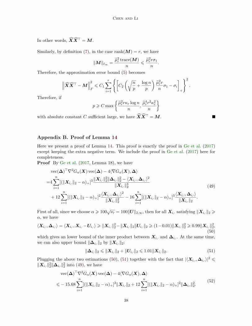
Chen and Li

In other words, XX> = M .

Similarly, by definition (7), in the case rank(M) = r, we have

‖M‖`∞ =µ2r trace(M)

n6µ2rrσ1

n.

Therefore, the approximation error bound (5) becomes∥∥∥XX> −M∥∥∥2

F6 C1

r∑i=1

[C2

(√n

p+

log n

p

)µ2rr

nσ1 − σi

]+

2

.

Therefore, if

p > C max

µ2rrκr log n

n,µ4rr

2κ2r

n

with absolute constant C sufficient large, we have XX> = M .

Appendix B. Proof of Lemma 14

Here we present a proof of Lemma 14. This proof is exactly the proof in Ge et al. (2017)except keeping the extra negative term. We include the proof in Ge et al. (2017) here forcompleteness.Proof By Ge et al. (2017, Lemma 18), we have

vec(∆)>∇2Gα(X) vec(∆)− 4〈∇Gα(X),∆〉

=4n∑i=1

[(‖Xi,·‖2 − α)+]3‖Xi,·‖22‖∆i,·‖22 − 〈Xi,·,∆i,·〉2

‖Xi,·‖32

+ 12n∑i=1

[(‖Xi,·‖2 − α)+]2〈Xi,·,∆i,·〉2

‖Xi,·‖22− 16

n∑i=1

[(‖Xi,·‖2 − α)+]3〈Xi,·,∆i,·〉‖Xi,·‖2

.

(49)

First of all, since we choose α > 100√νr = 100‖U‖2,∞, then for all Xi,· satisfying ‖Xi,·‖2 >

α, we have

〈Xi,·,∆i,·〉 = 〈Xi,·,Xi,·−Ui,·〉 > ‖Xi,·‖22−‖Xi,·‖2‖Ui,·‖2 > (1−0.01)‖Xi,·‖22 > 0.99‖Xi,·‖22,(50)

which gives an lower bound of the inner product between Xi,· and ∆i,·. At the same time,we can also upper bound ‖∆i,·‖2 by ‖Xi,·‖2:

‖∆i,·‖2 6 ‖Xi,·‖2 + ‖Ui,·‖2 6 1.01‖Xi,·‖2. (51)

Plugging the above two estimations (50), (51) together with the fact that |〈Xi,·,∆i,·〉|2 6‖Xi,·‖22‖∆i,·‖22 into (49), we have

vec(∆)>∇2Gα(X) vec(∆)− 4〈∇Gα(X),∆〉

6− 15.68n∑i=1

[(‖Xi,·‖2 − α)+]3‖Xi,·‖2 + 12

n∑i=1

[(‖Xi,·‖2 − α)+]2‖∆i,·‖22.(52)

38


Moreover, for all Xi,· satisfies ‖Xi,·‖2 > 5α, we can also upper bound ‖∆i,·‖2 by ‖Xi,·‖2:

‖∆i,·‖2 6 ‖Xi,·‖2 + ‖Ui,·‖2 6 1.002‖Xi,·‖2, (53)

and also lower bound ‖Xi,·‖2 − α by ‖∆i,·‖2:

‖Xi,·‖2 − α >

(1− 1

5

)‖Xi,·‖2 >

400

501‖∆i,·‖2. (54)

Plugging (53) and (54) back to (52), we have

vec(∆)>∇2Gα(X) vec(∆)− 4〈∇Gα(X),∆〉

612∑

i,‖Xi,·‖2<5α

[(‖Xi,·‖2 − α)+]2‖∆i,·‖22

+

[12− 15.68× 400

501× 1

1.002

] ∑i,‖Xi,·‖2>5α

[(‖Xi,·‖2 − α)+]2‖∆i,·‖22

6192α2‖∆‖2F − 0.3∑

i,‖Xi,·‖2>5α

‖∆i,·‖42

6199.54α2‖∆‖2F − 0.3n∑i=1

‖∆i,·‖42,

where the last inequality uses the fact that ‖∆i,·‖2 6 ‖Xi,·‖2 + ‖Ui,·‖2 and α > 100√νr.

39

model-free nonconvex matrix completion: local minima

Documents