Modeling, Identification and Control, Vol. 36, No. 3, 2015, pp. 179–188, ISSN 1890–1328

Model-free optimal anti-slug control of awell-pipeline-riser in the K-Spice/LedaFlow

simulator

Christer Dalen 1 David Di Ruscio 1 Roar Nilsen 2

1Telemark University College, P.O. Box 203, N-3901 Porsgrunn, Norway.

2Kongsberg Oil & Gas Technologies, Norway.

Abstract

Simplified models are developed for a 3-phase well-pipeline-riser and tested together with a high fidelitydynamic model built in K-Spice and LedaFlow. These models are developed from a subspace algorithm,i.e. Deterministic and Stochastic system identification and Realization (DSR), and implemented in aLinear Quadratic optimal Regulator (LQR) for stabilizing the slugging regime. We are comparing LQRwith PI controller using different performance measures.

Keywords: optimal controller, integral action, PI controller, Kalman filter, system identification, anti-slug, well-pipeline-riser

1 Introduction

In the offshore industry, multiphase transportationpipelines, which parts may consist of one or severalrisers, can introduce a set of different flow patterns,in particular; ‘Severe slugging’. The signature of‘Severe slugging’ phenomenon is large pressure andflow oscillations, and it is of great interest to stabilizethis flow regime since it may endanger personnel andequipment, as well to reduce production rate.

A subset of papers proposing different anti-slug con-trol solutions, is bulleted below:

• Introduced gaslift at riser base as control input,controlling riser base pressure, inAlvarez and Al-Malki (2003).

• Feedback PID control strategy of a pipeline-riser,controlling the riser base pressure with the topsidechoke as control input, in Ogazi AI (2010), Jahan-shahi and Skogestad (2015), Storkaas and Skoges-tad (2007), Storkaas et al. (2001) and Skogestad(2009).

• Cascade control strategies of a well-subsea-riser,controlling riser base pressure with topside- andsubsea choke, in Godhavn et al. (2005)

In this paper we will not use any models developedfrom mechanistic rules, actually, since the controllingresults presented in this paper evolve only from a col-lection of data we may refer to this solution as Model-Free Control (MFC), a concept contained in Di Ruscio(2012). The previous mentioned paper demonstratesMFC on a lab-scale quadruple tank process using anLQR optimal controller. The proposed controller usedis optimal in the sense that a standard linear quadraticperformance index is minimized. The essential prob-lem in this paper will be to identify system matrices fora linear state space model, using a subspace algorithm,i.e. DSR (Di Ruscio (1996)). The DSR algorithm hasshown good performance over other algorithms, com-pared on an activated sludge process (Sotomayor et al.(2003)).The main contributions of this paper are itemized asfollows:

• System identification approach on the well-

doi:10.4173/mic.2015.3.5 c© 2015 Norwegian Society of Automatic Control

Modeling, Identification and Control

pipeline-riser example, using a subspace algo-rithm.

• Model-free optimal anti-slug control of 3 differentcases, each described in Section 4.

A most valuable tool for investigating such sluggingbehavior, has been to use the ‘state-of-art’, modellingtools; LedaFlow multiphase flow simulator (LedaFlow)integrated with a K-Spice dynamic process simulator(K-Spice), developed and used by Kongsberg Oil & GasTechnologies for the last 30 years in the oil and gas in-dustry. K-Spice and LedaFlow are high fidelity simula-tors and are well suited to investigate the real offshorewell, pipeline, riser and topside process integrated inone dynamic model. LedaFlow is an independent andopen simulator that is the first to provide slug captur-ing and the only solution that predicts hydrodynamicslugs.

Enumerated as in sections, the paper is organized asfollows:

1. In the introduction we present the anti-slug prob-lem, past solutions and our contributions.

2. In the process description we describe the well-pipeline-riser.

3. In the theory section we define the system model,the problem and the functions which the results ofthis paper rest upon.

4. In the simulations section we identify models andimplement them in a model-free optimal anti slugcontrol for three different cases.

5. Some concluding remarks.

2 Process Description

A 3-phase well-pipeline-riser example integrated in theK-Spice/LedaFlow simulator is studied in this paper.This example has 3 manipulative inputs of interest forcontrolling flow/pressure; Topside choke, Subsea chokeand Gaslift. Together with the sentences itemized be-low, the pipeline profile; Fig. 1 gives a brief descriptionof the process example.

• Outputs

{y1: Outlet flow, FT100, [kg/s]

y2: Riser pressure, PT006, [bara]

where y1 ∈ [0, 100] and y2 ∈ [0, 200]. Notethat y2: Riser pressure is the pressure in thebottom of the riser as illustrated in Fig. 1.

x

y

−1 0 1 2 3 4 5

−5

−4

−3

−2

−1

0

1

2

[km]

[km]

u1

u2

u3

y1

y2

A

C

B

Figure 1: Illustration of the 3-phase well-pipeline-riserprocess integrated in the K-Spice/LedaFlowsimulator.

• Inputs

u1: Topside choke, HC001, [%]

u2: Subsea choke, V-HCV1, [%]

u3: Gaslift choke, FIC001, [%]

where ui ∈ [0, 100] ∀ i = 1, 2, 3.

• Stream-constrains

A: 25 [bara]

B: 500 [bara], 100[◦C]

C: 120 [bara], 30[◦C]

Note that bara is the absolute pressure expressedin bar, where 0 bara is associated with total vac-cum.

• Gaslift stabilize the production flow rate by de-creasing the density and increasing the flow rate.

3 Theory

Definition 3.1 (System model)We assume that the underlying system can be describedby a Linear discrete Time-Invariant (LTI) State SpaceModel (SSM) of following form

180

Christer Dalen, “Model-free optimal anti-slug control”

xk+1 = Axk + Buk + Cek

{Initial predicted state

x0

,

yk = Dxk + Euk + Fek,

(1)

where k ∈ N is the discrete time, xk ∈ Rn is thepredicted state vector, uk ∈ Rr is the input vector, yk ∈Rm is the output vector and ek ∈ Rm is white noisewith unit covariance matrix, i.e. E(eke

Tk ) = I. We

may have the model in a traditional way by writing thecommon Kalman filter on innovations form, i.e.

xk+1 = Axk + Buk + Kεk

{Initial predicted state

x0

,

yk = Dxk + Euk + εk,

(2)

where εk = Fek is the innovations process, K = CF−1

is the Kalman filter gain matrix and E(εkεTk ) = FFT

is the the innovations covariance matrix. Note thatin this paper we have forced the feed-through matrix,E = 0, by setting g = 0 which is shown in Eq. 8.

Definition 3.2 (System Identification Problem)From known input and output time series, the problemis to identify a state space model, i.e the followingsystem matrices (A,B,C,D,E, F ) in Eq. 1 and theinitial state x0. The time series

uk

yk

}∀ k = 1, . . . , N,

are organized as output and input matrices, respec-tively

Y =

yT1yT2...yTN

∈ RN×m, U =

uT1

uT2...

uTN

∈ RN×r. (3)

It is important to note that we are using centereddata, i.e. uk := uk − u0 and yk := yk − y0, where

y0 =1

N

N∑k=1

yk, (4)

u0 =1

N

N∑k=1

uk. (5)

The removing of trends from the data will often in-crease the accuracy of the estimated model.

Definition 3.3 (Functions)A set of functions are itemized below, essentially, the

problems considered in this paper are solved, in MAT-LAB, by combining members from this set, structuredinside (nested) for-loop(s). We may associate theMATLAB scripts with the function diagrams/block di-agrams shown in Figs. 2, 3 and 4.

• Pseudo Random Binary Sequence (PRBS), aMATLAB function designed as

U = prbs1(N,Tmin, Tmax), (6)

where U is as defined in Eq. 3 and uk ∈{−1, 1} ∀ k = 1, . . . , N . The signal uk is PRBSsuch as the constant intervals Ti are random inthe interval Tmin ≤ Ti ≤ Tmax. See e.g. Fig. 6.The reason for using a PRBS excitation signal isthat we want to be able to identify a model withsufficiently high order n. Notice, that a pure stepsignal only is persistently exciting of order n = 1,Soderstrom and Stoica (1989).

• Deterministic and Stochastic system identificationand Realization, (DSR) Di Ruscio (1996). Themodel matrices in Eqs.1,2 are identified using thefollowing MATLAB function:

[A,B,D,E,C, F, x0]

= dsr(Y,U, L, g, J,M, n)(7)

where

L : 1 ≤ L : Future horizon

g : Structure parameter

Note that g = 0 gives E = 0.

J : L ≤ J : Past horizon

n : 0 < n ≤ Lm : Number of states

M : M = 1 is default, a dummy parameter

(8)

• Mean Square Error (MSE):

MSE =1

N

N∑k=1

(yk − ydk)2 , (9)

where ydk is the output of the deterministic part ofthe model

xdk+1 = Axd

k + Buk,

ydk = Dxdk,

(10)

and with initial state xd1 = x0.

• Linear Quadratic Regulator (LQR), Di Ruscio(2012):

uk = uk−1 + G1∆xk + G2(yk−1 − rk), (11)

181

Modeling, Identification and Control

where the state deviation ∆xk = xk − xk−1 andrk ∈ Rm is the reference for the output y. A MAT-LAB script calculates the optimal feedback matri-ces: [G1, G2] = dlqdu pi(A,B,D,Q, P ), where Qand P are the weighting matrices for respectivelyreference tracking and control deviation.

• State observer for state deviation, Di Ruscio(2012), evolved from Eq. 2, are

∆xk+1 = A∆xk + B∆uk

+ K(yk − yk−1 −D∆xk),

Initial state

deviation

∆x1 = 0

(12)

where ∆uk = uk − uk−1. The model matrices(A,B,D,K) are identified from DSR, i.e. fromEq. 7 with K = CF−1.

• Integrated Absolute Error (IAE):

IAE =

∫ ∞0

|r − y|dt (13)

We may calculate the IAE recursively, as shownin Di Ruscio (2010), in discrete time: IAEk+1 =IAEk + ∆t|rk − yk|, where ∆t is the samplingtime.

• Total Value (TV):

TV =

∞∑k=1

|∆uk|, (14)

where, ∆uk = uk − uk−1, is the control rate ofchange.

PRBS Processuk yk

Figure 2: Block diagram of the proposed membersworking together through iterations of k,bounded as 1 ≤ k ≤ N , to produce the inputand output data, uk and yk, which is to beorganized in matrices, Y and U as in Eq. 3.The PRBS block is as Eq. 6.

Definition 3.4 (Notation)Because of some untraditional linguistics used throughthis paper, it is convenient, for not confusing thereader, to give some additional definitions.

DSR

Simulate

U

MSE

Y

Is minimum

L, n, J, Y, U A,B,C,D,E, F, x0

Ys

MSE

Figure 3: Block diagram of the proposed mem-bers working together through iterations ofL, n, J , each bounded as described in Eq. 8.The optimal model, meaning the model giv-ing the lowest MSE, is choosen. The ‘DSR’block is as Eq. 7 and the ‘MSE’ block is asEq. 9.

LQR Processuk

State observer

rk yk−

yk−1 ∆xk xk

Figure 4: Block diagram of the proposed membersworking together through iterations of k,bounded as 1 ≤ k ≤ N , to control yk. The‘LQR’ block is as Eq. 11 and the ‘State esti-mator’ block is as Eq. 12.

182

Christer Dalen, “Model-free optimal anti-slug control”

• Real process := K-Spice/LedaFlow simulator

• Model := model identified from the DSR subspacealgorithm

• @ := around or working point

4 Simulation Results

4.1 Introduction

We present three cases for which we have appliedMFC, where our goal is to control/stabilize the out-let flow. The sampling time is ∆t = 1 sec., how-ever different simulation speeds may be used in theK-Spice/LedaFlow simulator. The steps performed ineach case is enumerated below.

1. Identify an interesting operating point, i.e. a pointwhere severe slugging is present.

2. Collect datasets from an input experiment, Fig. 2.

3. Identify model, Fig. 3.

4. Control process, Fig. 4.

4.2 Case A: Topside choke and introducedGas lift

Introducing gaslift is said to to be the most effectiveway of stabilizing the slugging regime. Considering theopen-loop simulation (Fig. 5), we see that introducinggaslift is stabilizing the flow.We define the case as

y ∈ R :={y1: Outlet flow [kg/s] ,

u ∈ R2 :=

{u1: Topside choke @ 25 [%]

u3: Gaslift choke @ 1.5 [%].

Inputs and outputs were collected into U ∈ RN×2

and Y ∈ RN (Fig. 6), where N = 3600 samples. Thefirst 125 samples was removed, thereafter the setwas divided into 2/3 for identification and 1/3 forvalidation.

It was observed that using both inputs u1 andu3 gave a higher order model, and worse predictionerror than if we just used u3, hence we will assume asingle-input and single-output (SISO) model with u3

as input and set u1 = 25.25. The model is identifiedwith DSR-parameters; L = 7, J = 12, n = 5.

0 500 1000 1500 2000 2500 3000

y1

25

30

35

40

45

50y

1: Outlet flow [kg/s]

Time [Samples]0 500 1000 1500 2000 2500 3000

u3

0

1

2

3

4

5

6u

3: Gaslift choke [%]

Figure 5: Open-loop simulations in K-Spice. Introduc-ing the Gaslift choke at Time = 1000 Sam-ples. Topside choke was kept constant atu1 = 25. Case A

0 500 1000 1500 2000 2500 3000 3500

y1

25

30

35

40

45y

1 : Outlet flow [kg/s]

0 500 1000 1500 2000 2500 3000 3500

u1

24.5

25

25.5

26u

1 : Topside choke [%]

Time [Samples]0 500 1000 1500 2000 2500 3000 3500

u3

0.5

1

1.5

2

2.5u

3 : Gaslift choke [%]

Figure 6: When stepping the topside choke and gasliftvalve, the input and output series were col-lected from the K-Spice model, with a lengthof N = 3600 samples. These inputs are froman experimental design, i.e. PRBS as in Eq.6 where Tmin = 20 and Tmax = 120. Theseresults are from a MATLAB script associatedwith the block diagram in Fig. 2. The sim-ulation speed in K-Spice was 30 times realtime. Case A

183

Modeling, Identification and Control

Time [Samples]0 500 1000 1500 2000 2500

y1

-10

-5

0

5

10

15y

1: Outlet flow, FT100 [kg/s]

RealModel

Figure 7: Model (L = 7, J = 12, n = 5) simulatedand compared to the identification set, givingMSE = 1.0777. Results from a MATLABscript associated with Fig. 3. Case A

A =

Identified SISO model︷ ︸︸ ︷0.9900 −0.4930 −0.0260 −0.1033 −0.07690.0162 0.9907 0.7521 −0.2880 0.5406−0.0005 −0.0006 0.6030 0.7346 0.1834−0.0002 0.0012 −0.3761 0.0323 0.9153−0.0001 0.0003 0.1408 −0.5039 −0.1200

B =

−0.57830.2534−0.0918−0.13060.0198

D =

[−0.3773 −0.5658 0.5351 −0.3387 0.3175

]

K =

−3.82260.6193−0.1150−0.1107−0.0488

The steady state gain is approximately 1.8 and the poles

are less than one in magnitude, hence the process is stable.

The model looks to have a good fit to the datasets, seeFigs. (Fig. 7) and (Fig. 8), moreover, the model is per-forming better over the validation set (MSE = 0.9330),than the identification set (MSE = 1.0777). Fig. 9 showsa successful implementation of the LQR, where the weightsare tuned (Q = 1 and P = 1000) using the identified model.We observe that the control input is moving on towards aconstant value after a given time. We are not surprised bythe good performance, since the model is proven good inboth identification and validation.

Time [Samples]0 200 400 600 800 1000 1200

y1

-8

-6

-4

-2

0

2

4

6

8

10y

1: Outlet flow, FT100 [kg/s]

RealModel

Figure 8: Model (L = 7, J = 12, n = 5) simulatedand compared to the validation set, givingMSE = 0.9330. Results from a MATLABscript associated with Fig. 3. Case A

0 500 1000 1500 2000 2500 3000

y2

31

32

33

34

35

36

37y

1 : Outlet flow [bara]

ReferenceLQ(Q=1,P=1000)

Time [Samples]0 500 1000 1500 2000 2500 3000

u3

0

1

2

3

4

5

6u

3 : Gaslift choke [%]

kg/s

Figure 9: Implementation in K-Spice of the optimalcontroller, LQR, controlling outlet flow, y1,with Gaslift choke u3. The weights are Q = 1and P = 1000. Results from a MATLABscript associated with Fig. 4. Case A

184

Christer Dalen, “Model-free optimal anti-slug control”

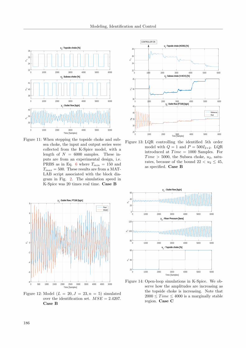
4.3 Case B: Topside choke and Subseachoke

Two manipulative input variables are chosen; Topsidechoke, u1, and Subsea choke, u2. Considering the open-loop simulations in Fig. 10 and some additional observa-tions, we will assume that the process is marginally stableat 22 < u1 ≤ 100 and 30 ≤ u2 ≤ 45. Hence, we definefollowing case as

y ∈ R :={y1: Outlet flow [kg/s] ,

u ∈ R2 :=

{u1: Topside choke @ 25 [%]

u2: Subsea choke @ 40 [%].

Input and output time-series were collected from an in-put experiment, (Fig. 11), and we identified a 5th ordermodel (Fig. 11), from the first 5000 samples, with DSR-parameters; L = 20, J = 23, n = 5, which gave minimumMSE = 2.4207 (Fig. 12).

A =

Identified MISO model︷ ︸︸ ︷0.9967 −0.1703 0.1552 −0.0712 −0.03250.0151 0.9997 0.3479 0.0511 0.2430−0.0005 0.0001 0.3659 0.6785 −0.41220.0000 −0.0002 −0.1975 0.7618 0.46380.0000 −0.0001 −0.0277 0.0477 0.7958

B =

−0.0713 −0.0501−0.1594 0.03260.3942 −0.0019−0.0033 0.00550.0304 −0.0087

D =

[−0.2114 −0.3619 0.8160 −0.1015 0.2399

]

K =

−5.36800.1029−0.4218−0.13360.0763

Fig. 13 shows the controlling results of the LQR, tuned

from trial-and-error methods. The LQR is introduced atT ime = 1000 and is in fact able to stabilize the outlet flowin the region which we assumed marginally stable. Notethat we have set the controller limits equal to this region.Despite how awful the model fits the identification set (Fig.12) we are actually achieving seemingly good controllingresults with the LQR.

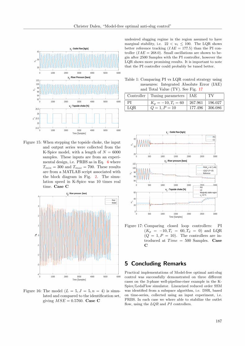
4.4 Case C: Topside choke

We choose to investigate a case with only the topside chokeas input variable. Considering the open-loop simulationsFig. 14 and some additional observations, we will assumethat the process is marginally stable at 22 < u1 ≤ 100.Hence, a case was constructed as

0 500 1000 1500 2000 2500 3000 3500 4000

u1

22

24

26

28u

1: Topside choke [%]

0 500 1000 1500 2000 2500 3000 3500 4000

u2

35

40

45u

2: Subsea choke [%]

Time [Samples]0 500 1000 1500 2000 2500 3000 3500 4000

y1

0

20

40

60y

1: Outlet flow [kg/s]

Figure 10: Open-loop simulations in K-Spice. Subseachoke looks to have a much higher steadystate gain than the topside choke. Case B

y ∈ R2 :=

{y1: Outlet flow [kg/s]

y2: Riser pressure [bara],

u ∈ R :={u1: Topside choke @ 25 [%] .

A 4th order SISO model, with only output y2, was iden-tified from the time-series (Fig. 15) with DSR-parameters;L = 5, J = 5, n = 4, with minimum MSE = 0.560 (Fig.16).

A =

Identified SISO model︷ ︸︸ ︷0.9984 −0.7044 0.4806 −0.51210.0039 0.9944 0.2759 0.86130.0000 −0.0026 −0.2460 1.1076−0.0001 0.0035 −0.6999 0.4946

B =

−0.0373−0.0010−0.0194−0.0080

D =

[−0.4462 −0.6336 0.6047 0.0857

]K =

−2.42890.62590.1498−0.1096

Fig. 17 shows successful implementations of two differ-

ent control strategies; LQR and PI. Both controllers aretuned using the identified model. The controllers are in-troduced at 500 Samples and are both able to stabilize the

185

Modeling, Identification and Control

0 1000 2000 3000 4000 5000 6000

u1

22

24

26

28u

1: Topside choke [%]

0 1000 2000 3000 4000 5000 6000

u2

39

40

41

u2: Subsea choke [%]

Time [Samples]0 1000 2000 3000 4000 5000 6000

y1

30

35

40

y1: Outlet flow [kg/s]

Figure 11: When stepping the topside choke and sub-sea choke, the input and output series werecollected from the K-Spice model, with alength of N = 6000 samples. These in-puts are from an experimental design, i.e.PRBS as in Eq. 6 where Tmin = 150 andTmax = 500. These results are from a MAT-LAB script associated with the block dia-gram in Fig. 2. The simulation speed inK-Spice was 20 times real time. Case B

Time [Samples]0 500 1000 1500 2000 2500 3000 3500 4000 4500 5000

y1

-8

-6

-4

-2

0

2

4

6

8y

1: Outlet flow, FT100 [kg/s]

RealModel

Figure 12: Model (L = 20, J = 23, n = 5) simulatedover the identification set. MSE = 2.4207.Case B

0 1000 2000 3000 4000 5000 6000

y2

25

30

35

40

45y

2: Outlet flow (FT100) [kg/s]

ReferenceReal

0 1000 2000 3000 4000 5000 6000

u1

22

24

26

28u

1: Topside choke (HC001) [%]

Time [Samples]

0 1000 2000 3000 4000 5000 6000

u2

35

40

45u

2: Subsea choke (V-HCV1) [%]

CONTROLLER ON

1

Figure 13: LQR controlling the identified 5th ordermodel with Q = 1 and P = 500I2×2. LQRintroduced at Time = 1000 Samples. ForTime > 5000, the Subsea choke, u2, satu-rates, because of the bound 22 < u2 ≤ 45,as specified. Case B

0 1000 2000 3000 4000 5000 6000

y1

0

20

40

60y

1 : Outlet flow [kg/s]

0 1000 2000 3000 4000 5000 6000

y2

80

100

120y

2 : Riser Pressure [bara]

Time [Samples]0 1000 2000 3000 4000 5000 6000

u1

20

40

60u

1 : Topside choke [%]

Figure 14: Open-loop simulations in K-Spice. We ob-serve how the amplitudes are increasing asthe topside choke is increasing. Note that2000 ≤ Time ≤ 4000 is a marginally stableregion. Case C

186

Christer Dalen, “Model-free optimal anti-slug control”

0 1000 2000 3000 4000 5000 6000

y1

30

35

40y

1: Outlet flow [kg/s]

0 1000 2000 3000 4000 5000 6000

y2

92

94

96

98

100

102y

2: Riser Pressure [bara]

Time [Samples]0 1000 2000 3000 4000 5000 6000

u1

24.5

25

25.5

26

26.5u

1: Topside choke [%]

Figure 15: When stepping the topside choke, the inputand output series were collected from theK-Spice model, with a length of N = 6000samples. These inputs are from an experi-mental design, i.e. PRBS as in Eq. 6 whereTmin = 300 and Tmax = 700. These resultsare from a MATLAB script associated withthe block diagram in Fig. 2. The simu-lation speed in K-Spice was 10 times realtime. Case C

Time [Samples]0 1000 2000 3000 4000 5000 6000

y1

-4

-3

-2

-1

0

1

2

3

4y

1: Outlet flow, FT100 [kg/s]

RealModel

Riser pressure [bara]2

Figure 16: The model (L = 5, J = 5, n = 4) is simu-lated and compared to the identification set,giving MSE = 0.5760. Case C

undesired slugging regime in the region assumed to havemarginal stability, i.e. 22 < u1 ≤ 100. The LQR showsbetter reference tracking (IAE = 177.5) than the PI con-troller (IAE = 268.0). Small oscillations are shown to be-gin after 2500 Samples with the PI controller, however theLQR shows more promising results. It is important to notethat the PI controller could probably be tuned better.

Table 1: Comparing PI vs LQR control strategy usingmeasures: Integrated Absolute Error (IAE)and Total Value (TV). See Fig. 17

Controller Tuning parameters IAE TV

PI Kp = −10, Ti = 60 267.961 196.027LQR Q = 1, P = 10 177.496 306.086

0 500 1000 1500 2000 2500 3000

y1

20

30

40

y1 : Outlet flow [kg/s]

PIDLQ

0 500 1000 1500 2000 2500 3000

y2

94

96

98

100

102y

2: Riser pressure [bara]

PID(Kp=-10,T

i=60)

LQ(Q=1,P=10)Reference

Time [Samples]0 500 1000 1500 2000 2500 3000

u1

0

20

40

60u

1 : Topside choke [%]

PIDLQMarginally stable regionu

1>22 %

Figure 17: Comparing closed loop controllers: PI(Kp = −10, Ti = 60, Td = 0) and LQR(Q = 1, P = 10). The controllers are in-troduced at Time = 500 Samples. CaseC

5 Concluding Remarks

Practical implementations of Model-free optimal anti-slugcontrol was successfully demonstrated on three differentcases on the 3-phase well-pipeline-riser example in the K-Spice/LedaFlow simulator. Linearized reduced order SSMwas identified from a subspace algorithm, i.e. DSR, basedon time-series, collected using an input experiment, i.e.PRBS. In each case we where able to stabilize the outletflow, using the LQR and PI controllers.

187

Modeling, Identification and Control

Acknowledgment

The authors acknowledge in bullets

• Kongsberg Oil & Gas Technologies for supporting withlicense and software for the K-Spice and LedaFlowsimulator.

• Telemark University College

MATLAB functions

The MATLAB functions used in this work are available foracademic use upon request.

References

Alvarez, C. and Al-Malki, S. Using gas injection for reduc-ing pressure losses in multiphase pipelines. InternationalJournal of Multiphase Flow, 2003. doi:10.2118/84503-MS.

Di Ruscio, D. Combined Deterministic and Stochas-tic System Identification and Realization: DSR - ASubspace Approach Based on Observations. Model-ing, Identification and Control, 1996. 17(3):193–230.doi:10.4173/mic.1996.3.3.

Di Ruscio, D. On Tuning PI Controllers for IntegratingPlus Time Delay Systems. Modeling, Identification andControl, 2010. 31(4):145–164. doi:10.4173/mic.2010.4.3.

Di Ruscio, D. Discrete LQ optimal control with inte-gral action: A simple controller on incremental form forMIMO systems. Modeling, Identification and Control,2012. 33(2):35–44. doi:10.4173/mic.2012.2.1.

Godhavn, J.-M., Fard, M. P., and Fuchs, P. H. Newslug control strategies, tuning rules and experimental re-

Godhavn, J.-M., Fard, M. P., and Fuchs, P. H. Newslug control strategies, tuning rules and experimental re-sults. Journal of Process Control, 2005. 15(5):547 – 557.doi:10.1016/j.jprocont.2004.10.003.

Jahanshahi, E. and Skogestad, S. Anti-slug con-trol solutions based on identified model. Jour-nal of Process Control, 2015. 30(0):58 – 68.doi:10.1016/j.jprocont.2014.12.007.

K-Spice. K-Spice. 2014. Kongsberg.com/k-spice.

LedaFlow. LedaFlow. 2014. Kongsberg.com/ledaflow.

Ogazi AI, Y. H. . L. L., Cao Y. Slug control with large valveopenings to maximize oil production. SPE Journal, 2010.15(3):812–821. doi:10.2118/124883-PA.

Skogestad, S. Feedback: Still the Simplest and BestSolution. Modeling, Identification and Control, 2009.30(3):149–155. doi:10.4173/mic.2009.3.5.

Soderstrom, T. and Stoica, P. System Identification. Pren-tice Hall, 1989.

Sotomayor, O. A., Park, S. W., and Garcia, C. Mul-tivariable identification of an activated sludge processwith subspace-based algorithms. Control EngineeringPractice, 2003. 11(8):961 – 969. doi:10.1016/S0967-0661(02)00210-1.

Storkaas, E. and Skogestad, S. Controllability analysis oftwo-phase pipeline-riser systems at riser slugging condi-tions. Control Engineering Practice, 2007. 15(5):567 –581. doi:10.1016/j.conengprac.2006.10.007.

Storkaas, E., Skogestad, S., and Alstad, V. Stabilisation ofdesired flow regimes in pipelines. AIChE Annual meeting,Chicago 1014 Nov., 1996, Paper 45f, 2001.

188