model-free stochastic collocation for an arbitrage-free ...maturity swaps (cms) consistently with...

Delft University of Technology

Model-free stochastic collocation for an arbitrage-free implied volatilityPart ILe Floch, Fabien; Oosterlee, Kees

DOI10.1007/s10203-019-00238-xPublication date2019Document VersionFinal published versionPublished inDecisions in Economics and Finance

Citation (APA)Le Floch, F., & Oosterlee, K. (2019). Model-free stochastic collocation for an arbitrage-free implied volatility:Part I. Decisions in Economics and Finance, 42(2), 679-714. https://doi.org/10.1007/s10203-019-00238-x

Important noteTo cite this publication, please use the final published version (if applicable).Please check the document version above.

CopyrightOther than for strictly personal use, it is not permitted to download, forward or distribute the text or part of it, without the consentof the author(s) and/or copyright holder(s), unless the work is under an open content license such as Creative Commons.

Takedown policyPlease contact us and provide details if you believe this document breaches copyrights.We will remove access to the work immediately and investigate your claim.

This work is downloaded from Delft University of Technology.For technical reasons the number of authors shown on this cover page is limited to a maximum of 10.

https://doi.org/10.1007/s10203-019-00238-x

Decisions in Economics and Finance (2019) 42:679–714https://doi.org/10.1007/s10203-019-00238-x

Model-free stochastic collocation for an arbitrage-freeimplied volatility: Part I

Fabien Le Floc’h1 · Cornelis W. Oosterlee1,2

Received: 23 July 2018 / Accepted: 8 February 2019 / Published online: 22 February 2019© The Author(s) 2019

AbstractThis paper explains how to calibrate a stochastic collocation polynomial againstmarketoption prices directly. The method is first applied to the interpolation of short-maturityequity option prices in a fully arbitrage-free manner and then to the joint calibrationof the constant maturity swap convexity adjustments with the interest rate swaptionssmile. To conclude, we explore some limitations of the stochastic collocation tech-nique.

Keywords Stochastic collocation · Implied volatility · Quantitative finance ·Arbitrage-free · Risk-neutral density

JEL Classification C630 · G170 · G130

1 Introduction

The market provides option prices for a discrete set of strikes and maturities. In orderto price over-the-counter vanilla options with different strikes, or to hedge more com-plex derivatives with vanilla options, it is useful to have a continuous arbitrage-freerepresentation of the option prices, or equivalently of their implied volatilities. Forexample, the variance swap replication of Carr and Madan consists in integrating aspecific function over a continuum of vanilla put and call option prices (Carr et al 1998;Carr and Lee 2008). An arbitrage-free representation is also particularly important forthe Dupire local volatility model (Dupire 1994), where arbitrages will translate to anegative implied variance.

A rudimentary, but popular representation is to interpolate market implied volatili-tieswith a cubic spline across option strikes. Unfortunately, itmay not be arbitrage-free

B Fabien Le Floc’[email protected]

1 Delft Institute of Applied Mathematics, TU Delft, Delft, The Netherlands

2 CWI-Centrum Wiskunde & Informatica, Amsterdam, The Netherlands

123

http://crossmark.crossref.org/dialog/?doi=10.1007/s10203-019-00238-x&domain=pdf

http://orcid.org/0000-0002-1142-8470

680 F. Le Floc’h, C. W. Oosterlee

as it does not preserve the convexity of option prices in general. Kahalé (2004) designsan arbitrage-free interpolation of the call prices. It, however, presents the followingdrawbacks: It requires convex input quotes and employs two embedded nonlinearminimizations, and it is not proven that the algorithm for the interpolation functionof class C2 converges. In reality, it is often not desirable to strictly interpolate optionprices as those fluctuate within a bid–ask spread. Interpolation will lead to a very noisyestimate of the probability density (which corresponds to the second derivative of theundiscounted call option price).

More recently, Andreasen and Huge (2011) have proposed to calibrate the discretepiecewise constant local volatility of the single-step finite difference representation forthe forward Dupire equation. In their representation, the authors use as many constantsas the number of market option strikes for an optimal fit. It works well but often yieldsa noisy probability density estimate, as the prices are overfitted.

An alternative is to rely on a richer underlying stochastic model, which allows forsome flexibility in the implied volatility smile, such as the Heston or SABR stochasticvolatility models. While semi-analytic representations of the call option price existfor the Heston model (Heston 1993), the model itself does not allow to representshort-maturity smiles accurately. The SABR model is better suited for this, but hasonly closed-form approximations for the call option price, which can lead to arbitrage(Hagan et al. 2002, 2014).

Grzelak and Oosterlee (2017) use stochastic collocation to fix the Hagan SABRapproximation formula defects and produce arbitrage-free option prices starting fromthe Hagan SABR formula. Here, we will explore how to calibrate the stochastic col-location polynomial directly to market prices, without going through an intermediatemodel.

This is of particular interest to the richer collocated local volatility (CLV) model,which allows to price exotic options throughMonte Carlo or finite difference methods(Grzelak 2016). A collocation polynomial calibrated to the vanilla options market iskey for the application of this model in practice.

Another application of our model-free stochastic collocation is to price constantmaturity swaps (CMS) consistently with the swaption implied volatility smile. In thestandard approximation of Hagan (2003), the CMS convexity adjustment consists inevaluating the second moment of the distribution of the forward swap rate. It can becomputed in closed form with the stochastic collocation. This allows for an efficientmethod to calibrate the collocation method jointly to the swaptions market impliedvolatilities and to the CMS spread prices.

The outline of the paper is as follows: Section 2 presents the stochastic colloca-tion technique in detail. Section 3 explains how to calibrate the stochastic collocationdirectly to market prices and how to ensure the arbitrage-free calibration transparently,through a specific parameterization of the collocation polynomial. Section 4 reviewssome popular option implied volatilities interpolation methods and illustrates the var-ious issues that may arise with those on a practical example. Section 5 applies thedirect collocation technique on two different examples of equity index option prices.Section 6 introduces the joint calibration of CMS convexity adjustments and swaptionprices in general. Section 7 applies the model-free stochastic collocation on the joint

123

Model-free stochastic collocation for an arbitrage-free… 681

calibration of CMS and swaption prices. Finally, Sect. 8 explores some limitations ofthe stochastic collocation technique along with possible remedies.

2 Overview of the stochastic collocationmethod

The stochastic collocation method (Mathelin and Hussaini 2003) consists in mappinga physical random variable Y to a point X of an artificial stochastic space. Collocationpoints xi are used to approximate the function1 mapping X to Y , F−1

X ◦ FY , whereFX , FY are, respectively, the cumulative distribution functions (CDF) of X and Y .Thus, only a small number of samples of Y (and evaluations of FY ) are used. Thisallows the problem to be solved in the “cheaper” artificial space.

In the context of option price interpolation, the stochastic collocation will allowus to interpolate the market CDF in a better set of coordinates. In particular, we willfollow (Grzelak and Oosterlee 2017) and use a Gaussian distribution for X .

In Grzelak andOosterlee (2017), the stochastic collocation is applied to the survivaldensity functionGY , whereGY (y) = 1−FY (y)with FY being the cumulative densityfunction of the asset price process. When the survival distribution function is knownfor a range of strikes, their method can be summarized by the following steps:

1. Given a set of collocation strikes yi , i = 0, . . . , N , compute the survival distribu-tion values pi at those points: pi = GY (yi ).

2. Project on the Gaussian distribution by transforming the pi using the inversecumulative normal distribution Φ−1 resulting in xi = Φ−1(1 − pi ).

3. Interpolate (xi , yi ) with a Lagrange polynomial gN .4. Price by integrating on the density with the integration variable x = Φ−1(1 −

GY (y)), using the Lagrange polynomial for the transform.

Let us now detail the last step. The undiscounted price of a call option of strike Kis obtained by integrating over the probability density function f , with a change ofvariable:

C(K ) =∫ +∞

0|y − K |+ f (y)dy (1)

=∫ Φ−1(1)

Φ−1(0)|G−1

Y (1 − Φ(x)) − K |+φ(x)dx

≈∫ ∞

−∞|gN (x) − K |+φ(x)dx

=∫ ∞

xK(gN (x) − K )φ(x)dx, (2)

where φ(x) is the Gaussian density function and

xK = g−1N (K ). (3)

The change of variables is valid when the survival density is continuous and its deriva-tive is integrable. In particular, it is not necessary for the derivative to be continuous.

1 A polynomial is often used for the mapping.

123


As shown in Hunt and Kennedy (2004), a polynomial multiplied by a Gaussian canbe integrated analytically as integration by parts leads to a recurrence relationship onmi (b) = ∫ ∞

b xiφ(x)dx . This idea is also the basis of the Sali tree method (Hu et al.2006). The recurrence is

mi+2(b) = (i + 1)mi (b) + bi+1φ(b), (4)

with m0(b) = Φ(−b),m1(b) = φ(b). We have then:

C(K ) =N∑i=0

aimi (xK ) − Φ(−xK )K , (5)

where ai are the coefficients of the polynomial in increasing powers.The terms mi (K ) involve only φ(xK ) and Φ(−xK ). The computational cost for

pricing one vanilla option can be approximated by the cost of finding xK and thecost of one normal density function evaluation plus one cumulative normal densityfunction evaluation. For cubic polynomials, xK can be found analytically throughCardano’s formula (Nonweiler 1968), and the cost is similar to the one of the Black–Scholes formulae. In the general case of a polynomial gN of degree N , the roots can becomputed in O(N 3) as the eigenvalues of the associated Frobenius companion matrixM defined by

M(gN ) =

⎛⎜⎜⎜⎜⎜⎜⎝

0 0 · · · 0 − a0aN

1 0 · · · 0 − a1aN

0 1 0 − a2aN

......

. . ....

...

0 0 · · · 1 − aN−1aN

⎞⎟⎟⎟⎟⎟⎟⎠

.

We have indeed det (λI − M) = gN (λ). This is, for example, how the Octave orMATLAB roots function works (Moler 1991). Note that for a high degree N , thesystem can be very ill-conditioned. A remedy is to use a more robust polynomial basissuch as the Chebyshev polynomials and compute the eigenvalues of the colleaguematrix (Good 1961; Trefethen 2011). Jenkins and Traub solve directly the problem offinding the roots of a real polynomial in Jenkins (1975).

A simple alternative, particularly relevant in our case as the polynomial needs to beinvertible and thus monotonic, is to use the third-order Halley’s method (Gander 1985)with a simple initial guess xK = −1 if K < F(0, T ) or xK = 1 if K ≥ F(0, T ), withF(0, T ) the forward price to maturity T . In practice, not more than three iterationsare necessary to achieve an accuracy around machine epsilon.

The put option price is calculated through the put-call parity relationship, namely

C(K ) − P(K ) = F(0, T ) − K ,

where P(K ) is the undiscounted price today of a put option of maturity T .

123


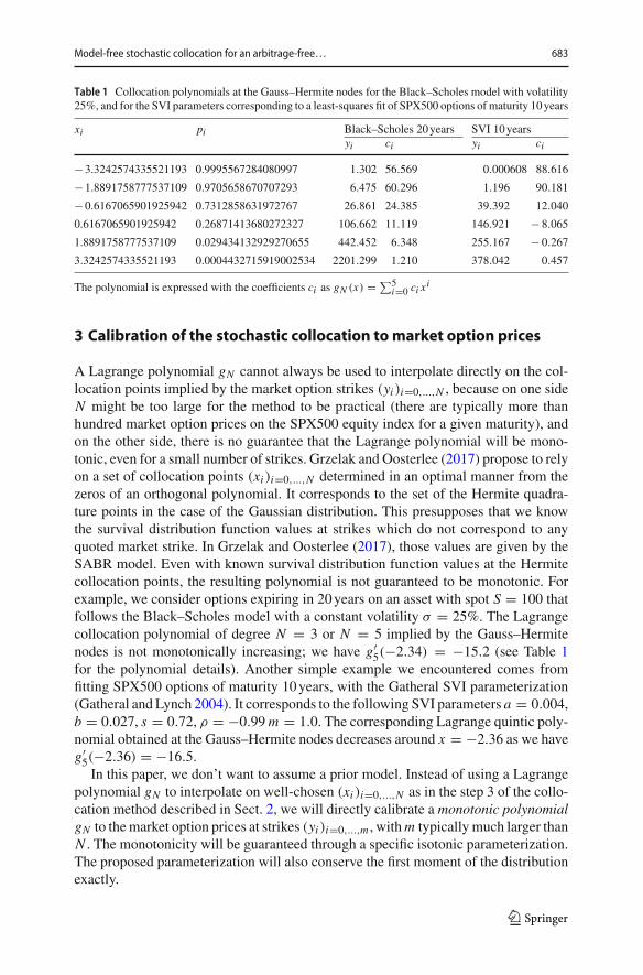
Table 1 Collocation polynomials at the Gauss–Hermite nodes for the Black–Scholes model with volatility25%, and for the SVI parameters corresponding to a least-squares fit of SPX500 options of maturity 10years

xi pi Black–Scholes 20years SVI 10yearsyi ci yi ci

−3.3242574335521193 0.9995567284080997 1.302 56.569 0.000608 88.616

−1.8891758777537109 0.9705658670707293 6.475 60.296 1.196 90.181

−0.6167065901925942 0.7312858631972767 26.861 24.385 39.392 12.040

0.6167065901925942 0.26871413680272327 106.662 11.119 146.921 − 8.065

1.8891758777537109 0.029434132929270655 442.452 6.348 255.167 − 0.267

3.3242574335521193 0.0004432715919002534 2201.299 1.210 378.042 0.457

The polynomial is expressed with the coefficients ci as gN (x) = ∑5i=0 ci x

i

3 Calibration of the stochastic collocation tomarket option prices

A Lagrange polynomial gN cannot always be used to interpolate directly on the col-location points implied by the market option strikes (yi )i=0,...,N , because on one sideN might be too large for the method to be practical (there are typically more thanhundred market option prices on the SPX500 equity index for a given maturity), andon the other side, there is no guarantee that the Lagrange polynomial will be mono-tonic, even for a small number of strikes. Grzelak and Oosterlee (2017) propose to relyon a set of collocation points (xi )i=0,...,N determined in an optimal manner from thezeros of an orthogonal polynomial. It corresponds to the set of the Hermite quadra-ture points in the case of the Gaussian distribution. This presupposes that we knowthe survival distribution function values at strikes which do not correspond to anyquoted market strike. In Grzelak and Oosterlee (2017), those values are given by theSABR model. Even with known survival distribution function values at the Hermitecollocation points, the resulting polynomial is not guaranteed to be monotonic. Forexample, we consider options expiring in 20years on an asset with spot S = 100 thatfollows the Black–Scholes model with a constant volatility σ = 25%. The Lagrangecollocation polynomial of degree N = 3 or N = 5 implied by the Gauss–Hermitenodes is not monotonically increasing; we have g′

5(−2.34) = −15.2 (see Table 1for the polynomial details). Another simple example we encountered comes fromfitting SPX500 options of maturity 10years, with the Gatheral SVI parameterization(Gatheral and Lynch 2004). It corresponds to the following SVI parameters a = 0.004,b = 0.027, s = 0.72, ρ = −0.99m = 1.0. The corresponding Lagrange quintic poly-nomial obtained at the Gauss–Hermite nodes decreases around x = −2.36 as we haveg′5(−2.36) = −16.5.In this paper, we don’t want to assume a prior model. Instead of using a Lagrange

polynomial gN to interpolate on well-chosen (xi )i=0,...,N as in the step 3 of the collo-cation method described in Sect. 2, we will directly calibrate a monotonic polynomialgN to themarket option prices at strikes (yi )i=0,...,m , withm typicallymuch larger thanN . The monotonicity will be guaranteed through a specific isotonic parameterization.The proposed parameterization will also conserve the first moment of the distributionexactly.

123


In order to apply the stochastic collocation directly to market option prices, we thusneed to:

– find an estimate of the survival density from the market option prices (correspond-ing to the step 1 of the collocation method described in Sect. 2),

– find a good initial guess for the monotonic polynomial gN ,– optimize the polynomial coefficients so that the collocation prices are closest tothe market option prices.

We will detail each step.

3.1 A rough estimate of themarket survival density

Kahalé (2004) proposes a straightforward estimate. Let (yi )i=0,...,m be the marketstrikes and (ci )i=0,...,m the market call option prices corresponding to each strike; thecall price derivative c′

i toward the strike Ki can be estimated by

c′i ≈ li + li+1

2where li = ci − ci−1

yi − yi−1(6)

for i = 1, . . . ,m − 1, and with c′0 = l1, c′

m = lm .If the market prices are arbitrage-free, that is when

− 1 <ci − ci−1

yi − yi−1<

ci+1 − ciyi+1 − yi

< 0, for i = 1, . . . ,m − 1 (7)

it is guaranteed that −1 < c′i < 0 and the c′

i are increasing. A more precise estimateconsists in using the parabola that passes through the three points ci−1, ci , ci+1 toestimate the slopes:

c′i ≈ li (yi+1 − yi ) + li+1(yi − yi−1)

yi+1 − yi−1where li = ci − ci−1

yi − yi−1(8)

for i = 1, . . . ,m − 1, and with c′0 = l1, c′

m = lm . It will still lead to −1 < c′i < 0 and

increasing c′i .

We can build a continuous representation of the survival density by interpolatingthe call prices (yi , ci )i=0,...,m with theC1 quadratic spline interpolation of Schumaker(1983), where additional knots are inserted to preserve monotonicity and convexity.2

By construction, at each market strike, the derivative will be equal to each c′i .

The survival density corresponds to

GY (y) = −∂C

∂ y(y), (9)

2 AC1 polynomial spline on a fixed set of knots cannot preserve monotonicity and convexity in the generalcase (Passow and Roulier 1977).

123


or equivalently through the put option prices P:

GY (y) = 1 − ∂P

∂ y(y). (10)

In practice, one will use out-of-the-money options to compute the survival densityusing alternative Eqs. (9) and (10).While in the case of the SABRmodel, it is importantto integrate the probability density (or the second derivative of the call price) from yto ∞ (Grzelak and Oosterlee 2017), here we are only interested in a rough guess.3

From the survival density at the strikes yi , it is then trivial to compute the normalcoordinates xi .

3.2 Filtering out themarket call prices quotes

In reality, it is not guaranteed that the market prices are convex, because of the bid–askspread. While the collocation calibration method we propose in this paper will stillwork well on a nonconvex set of call prices, starting the optimization from a convexset has two advantages: a better initial estimate of the survival density and thus a betterinitial guess, and the use of a monotonic interpolation of the survival density.

The general problemof extracting a “good”, representative convex subset of a nearlyconvex set is not simple. By “good”, we mean, for example, that the frontier definedby joining each point of the set with a line minimizes the least-squares error on thefull set, along with possibly some criteria to reduce the total variation. In Appendix C,we propose a quadratic programming approach to build a convex set that closelyapproximates the initial set of market prices. It can, however, be relatively slow whenthe number of market quotes is large. The algorithm takes 4.8 s on a Core i7 7700U,for the 174 SPX500 option prices as of January 23, 2018, from our example in Sect. 5.

A much simpler approach is to merely filter out problematic quotes, i.e., quotesthat will lead to a call price derivative estimate lower than −1 or positive. We assumethat the strikes (yi )0≤i≤m are sorted in ascending order. The algorithm starts from aspecific index k ∈ {0, . . . ,m}. We will use k = 0, but we let the algorithm to be moregeneric. The forward sweep to filter out problematic quotes consists then in:

(i) Start from strike yk . Let the filtered set be S = {(yk, xK )}. Let j� = k,(ii) Search for the next lowest index j , such that −1 + ε <

c j−c j�y j−y j�

< −ε and j� <

j ≤ m. Replace j� by j ,(iii) Add (y j� , c j� ) to the filtered set S . Repeat steps (ii) and (iii).

In our examples, we set the tolerance ε = 10−7 to avoid machine epsilon accuracyissues close to − 1. A small error in the derivative estimate near − 1 or near 0 willlead to a disproportionally large difference in the coordinate x .

While the above algorithm will not produce a convex set, we will see that it can besurprisingly effective to compute a good initial guess for the collocation polynomial.

3 Integration is still possible with the quadratic spline interpolation approach.

123


We could also derive a similar backward sweep algorithm and combine the twoalgorithms to start at the strike yk close to the forward price F(0, T ). On our examples,this was not necessary.

3.3 An initial guess for the collocation polynomial

In order to obtain an arbitrage-free price, it is not only important that the density(zeroth moment) sums up to 1, which the collocation method will obey by default, butit is also key to preserve the martingale property (the first moment), that is

∫ ∞

−∞gN (x)φ(x) = F(t, T ). (11)

Using the recurrence relation [Eq. (4)], this translates to

a0 +N−12∑

i=1

a2i (2i − 1)!! = F(t, T ). (12)

Instead of trying to find directly good collocation points, a simple idea for an initialguess is to consider the polynomial hN (x) = ∑N

k=0 bkxk corresponding to the least-

squares fit of xi , yi :

b0, . . . , bN = min(a0,...,aN )∈RN+1

⎧⎨⎩

m∑i=0

[(N∑

k=0

akxki

)− yi

]2⎫⎬⎭ , (13)

with the additional martingality constraint. This is a linear problem and is very fastto solve, for example, by QR decomposition. Unfortunately, the resulting polynomialmight not be monotonic.

As we want to impose the monotonicity constraint by a clever parameterization ofthe problem, wewill only consider the least-squares (with additional martingality con-straint) cubic polynomial as starting guess. The following lemma helps us determinewhether it is monotonic.

Lemma 1 A cubic polynomial a0 + a1x + a2x2 + a3x3 is strictly monotonic andincreasing on R if and only if a22 − 3a1a3 < 0.

Proof The derivative has no roots if and only if the discriminant a22 − 3a1a3 < 0 If our first attempt for a cubic initial guess is not monotonic, we follow the idea

of Murray et al. (2016) and fit a cubic polynomial of the form A+ Bx +Cx3. For thisspecific case, the linear system to solve is then given by

⎛⎝1 0 00

∑mi=0x

2i

∑mi=0x

4i

0∑m

i=0x4i

∑mi=0x

6i

⎞⎠

⎛⎝ABC

⎞⎠ =

⎛⎝ F(t, T )∑m

i=0xi yi∑mi=0x

3i yi

⎞⎠ . (14)

123


In our case, Lemma 1 reduces to B > 0 and C > 0. As the initial guess, we thususe the cubic polynomial with coefficients a0 = A = F(t, T ), a1 = |B|, a2 = 0,a3 = |C |.

3.4 Themeasure

The goal is to minimize the error between specific model implied volatilities andthe market implied volatilities, taking into account the bid–ask spread. The impliedvolatility error measure corresponds then to the weighted root-mean-square error ofimplied volatilities:

Mσ =√∑m

i=0 μ2i (σ (ξ, Ki ) − σi )

2

√∑mi=0 μ2

i

, (15)

where σ(ξ, Ki ) is the Black implied volatility4 obtained from the specific modelconsidered, with parameters ξ , σi is the market implied volatility and μi is the weightassociated with the implied volatility σi . In our numerical examples, we will chooseμi = 1. In practice, it is typically set as the inverse of the bid–ask spread.

An alternative is to use the root-mean-square error of prices:

MV =√∑m

i=0 w2i (C(ξ, Ki ) − ci )2√∑m

i=0 w2i

, (16)

where C(ξ, Ki ) is the model5 option price and ci is the market option price at strikeKi . We can find a weight wi that makes the solution similar to the one under themeasure Mσ by matching the gradients of each problem. We compare

m∑i=0

2w2i∂C

∂ξ(ξ, Ki ) (ci − C(ξ, Ki )) ,

withm∑i=0

2μi2 ∂σ

∂ξ(ξ, Ki ) (σi − σ(ξ, Ki )) .

As we know that ∂C∂ξ

= ∂σ∂ξ

∂C∂σ

, we approximate ∂C∂σ

by the market Black–Scholes

Vega, the term (ci − C(ξ, Ki )) by ∂C∂ξ

(ξopt − ξ), and (σi − σ(ξ, Ki )) by ∂σ∂ξ

(ξopt − ξ)

to obtain

wi ≈ 1∂ci∂σi

μi . (17)

4 Fast and robust algorithms to obtain the implied volatility from an option price are given in Jäckel (2015)and Li and Lee (2011).When no implied volatility corresponds to the model option price, which can happenbecause of numerical error, we just fix the implied volatility to zero.5 In the case of the stochastic collocation, ξ corresponds to the coefficients of the collocation polynomial.

123


In practice, the inverse Vega needs to be capped to avoid taking into account toofar out-of-the-money prices, which won’t be all that reliable numerically and we take

wi = min

(1

νi,106

F

)μi , (18)

where νi = ∂ci∂σ

is the Black–Scholes Vega corresponding to the market option priceci .

3.5 Optimization under monotonicity constraints

Wewish to minimize the error measure MV while taking into account the martingalityand the monotonicity constraints (Lemma 1) at the same time. The polynomial gNis strictly monotonically increasing if its derivative polynomial is strictly positive.We follow the central idea of Murray et al. (2016) and express gN in an isotonicparameterization:

gN (x) = a0 +∫ x

0p(x)dx, (19)

where p(x) is a strictly positive polynomial of degree N − 1 = 2Q. It can thus beexpressed as a sum of two squared polynomials of respective degrees at most Q andat most Q − 1 (Reznick 2000):

p(x) = p1(x)2 + p2(x)

2. (20)

As in the case of the cubic polynomial, we can refine the initial guess by first findingthe optimal positive least-squares polynomial with the sum of squares parameteri-zation. Let (β1,0, . . . , β1,q) ∈ R

q+1 be the coefficients of the polynomial p1 and(β2,0, . . . , β2,q−1) ∈ R

q be the coefficients of the polynomial p2. The coefficients(γk)k=0,...,N−1 of p can be computed by adding the convolution of β1 with itself tothe convolution of β2 with itself, that is

γk =k∑

l=0

β1,lβ1,k−l +k∑

l=0

β2,lβ2,k−l , (21)

with β1,l = 0 for l > q and β2,l = 0 for l > q − 1. The martingality condition leadsto

gN (x) = F(t, T ) −N−12∑

k=1

γ2k−1

2k(2k − 1)!! +

N∑k=1

γk−1

kxk . (22)

123


Lemma 2 The gradient of gN toward (β1,0, . . . , β1,q , β2,0, . . . , β2,q−1) can be com-puted analytically, and we have

∂gN∂βl, j

(xi ) = 2q∑

k=0

βl,k xj+k+1i

k + j + 1−

q∑k=1

(2k − 1)!!k

βl,2k− j−1, (23)

with βl,k = 0 for k < 0 and β1,k = 0 for k > q and β2,k = 0 for k > q − 1.

Proof

gN (x) = a0 +∫ x

0

2q∑k=0

k∑l=0

β1,lβ1,k−l xk +

2q−2∑k=0

k∑l=0

β2,lβ2,k−l xkdx

= a0 +2q∑k=0

1

k + 1

k∑l=0

β1,lβ1,k−l xk+1 +

2q−2∑k=0

1

k + 1

k∑l=0

β2,lβ2,k−l xk+1.

We thus have

ak+1 ={

1k+1

(∑kl=0β1,lβ1,k−l + ∑k

l=0β2,lβ2,k−l

)for 0 ≤ k ≤ 2q − 2,

1k+1

∑kl=0β1,lβ1,k−l for k = 2q − 1, 2q.

We recall that the martingality condition implies

a0 = F(t, T ) −q∑

k=1

a2k(2k − 1)!!.

We have

∂a0∂βl, j

= −q∑

k=1

(2k − 1)!! ∂a2k∂βl, j

,

and

∂ak+1

∂β1, j= 1

k + 12β1,k− j for j ≤ k ≤ 2q,

∂ak+1

∂β2, j= 1

k + 12β2,k− j for j ≤ k ≤ 2q − 2,

∂ak+1

∂βl, j= 0 for k < j and l = 1, 2.

Thus,

∂a0∂βl, j

= −∑qk=1

(2k−1)!!k βl,2k− j−1,

123


with βl,k = 0 for k < 0 and β1,k = 0 for k > q and β2,k = 0 for k > q − 1.

In particular, for a cubic polynomial, we have

∂g3∂β1,0

(xi ) = 2β1,0xi + β1,1x2i − β1,1,

∂g3∂β2,0

(xi ) = 2β2,0xi ,

∂g3∂β1,1

(xi ) = β1,0x2i + 2β1,1

3x3i − β1,0,

and for a quintic polynomial,

∂g5∂β1,0

(xi ) = 2β1,0xi + β1,1x2i + 2β1,2

3x3i − β1,1,

∂g5∂β2,0

(xi ) = 2β2,0xi + β2,1x2i − β2,1,

∂g5∂β1,1

(xi ) = β1,0x2i + 2β1,1

3x3i + β1,2

2x4i − β1,0 − 3

2β1,2,

∂g5∂β2,1

(xi ) = β2,0x2i + 2β2,1

3x3i − β2,0,

∂g5∂β1,2

(xi ) = 2β1,0

3x3i + β1,1

2x4i + 2β1,2

5x5i − 3

2β1,1.

The cubic polynomial initial guess can be rewritten in the isotonic form as follows,

a0 + a1x + a2x2 + a3x

3 = a0 +∫ x

0

(a1 + 2a2t + 3a3t

2)dt

= a0 +∫ x

0

(√3a3t + a2√

3a3

)2

+⎛⎝

√a1 − a22

3a3

⎞⎠

2

dt .

(24)

Based on the initial guess (refined or cubic), we can use a standard unconstrainedLevenberg–Marquardt algorithm to minimize the measure MV , based on the iso-tonic parameterization. This results in the optimal coefficients (β1,0, . . . , β1,q) and(β2,0, . . . , β2,q−1), which we then convert back to a standard polynomial representa-tion, as described above.

The gradient of the call prices toward the isotonic parameters can also be computedanalytically from Eq. (2), as we have

∂C

∂βl, j(K ) = ∂xK

∂βl, j(K )C(K ) +

∫ ∞

xK

∂gN∂βl, j

(x)φ(x)dx,

123


where xK is the integration cutoff point defined by Eq. (3). As ∂gN∂x (β, xK ) > 0, we

can use the implicit function theorem to compute the partial derivatives ∂xK∂βl, j

(K ):

∇xK (β) = − 1∂gN∂x (β, xK )

∇gN (β, xK )

where ∇xK =(

∂xK∂β1,0

, . . . , ∂xK∂β2,q−1

)and ∇gN =

(∂gN∂β1,0

, . . . ,∂gN

∂β2,q−1

).

4 Examples of equity index smiles

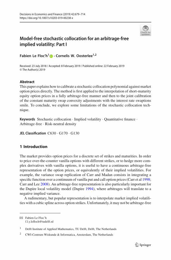
We consider a set of vanilla option prices on the same underlying asset, with the samematurity date. As an illustrating example, we will use SPX500 option quotes expiringon March 7, 2018, as of February 5, 2018, from Appendix D. The options’ maturityis thus nearly one month. The day before this specific valuation date, a big jump involatility across the whole stock market occurred. One consequence is a slightly moreextreme (but not exceptional) volatility smile.

4.1 A short review of implied volatility interpolations

Let us recall shortly some of the different approaches to build an arbitrage-free impliedvolatility interpolation, or equivalently, to extract the risk-neutral probability density.

We can choose to represent the asset dynamics by a stochastic volatility modelsuch as Heston (1993), Bates (1996), Double-Heston (Christoffersen et al. 2009).This implies a relatively high computational cost to obtain vanilla option prices andthus to calibrate the model, especially when time-dependent parameters are allowed.Furthermore, thosemodels are known to not fit adequately themarket of vanilla optionswith short maturities. Their implied volatility smile is typically too flat.

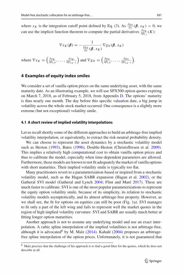
Many practitioners revert to a parameterization-based or inspired from a stochasticvolatility model, such as the Hagan SABR expansion (Hagan et al. 2002), or theGatheral SVI model (Gatheral and Lynch 2004; Flint and Maré 2017). These aremuch faster to calibrate. SVI is one of the most popular parameterizations to representthe equity option volatility smile, because of its simplicity, its relation to stochasticvolatility models asymptotically, and its almost arbitrage-free property. However, aswe shall see, the fit for options on equities can still be poor (Fig. 1a). SVI managesto fit only a part of the left wing and fails to represent well the market quotes in theregion of high implied volatility curvature. SVI and SABR are usually much better atfitting longer option maturities.

Another approach is not to assume any underlying model and use an exact inter-polation. A cubic spline interpolation of the implied volatilities is not arbitrage-free,although it is advocated6 by M. Malz (2014). Kahalé (2004) proposes an arbitrage-free spline interpolation of the option prices. Unfortunately, it is not guaranteed that

6 Malz precises that the challenge of his approach is to find a good filter for the quotes, which he does notdescribe at all.

123


20

30

40

50

60

70

2100 2400 2700

Strike

Impl

ied

vola

tility

in %

Method

Andreasen−Huge

Reference

SVI

(a) Implied volatility.

0.000

0.005

0.010

0.015

0.020

2100 2400 2700

Strike

Pro

babi

lity

dens

ity

Method

Andreasen−Huge

SVI

(b) Probability density.

Fig. 1 SVI and Andreasen–Huge calibrations on 1m SPX500 options as of February 05, 2018

his algorithm for C2 interpolation, necessary for a continuous probability density,converges. Furthermore, it assumes that the input call option quotes are convex anddecreasing by strike. But the market quotes are not convex in general, mainly becauseof the bid–ask spread. While we propose a quadratic programming-based algorithm tobuild a convex set that closely approximates the market prices in Appendix C, it canbe relatively slow when the number of quotes is large. Finally, the resulting impliedprobability density will be noisy, as evidenced by Syrdal (2002).

A smoothing spline or a least-squares cubic spline will allow to avoid overfittingthe market quotes. For example, Syrdal (2002) and Bliss and Panigirtzoglou (2004)

123


use a smoothing spline on the implied volatilities as a function of the option deltas,7

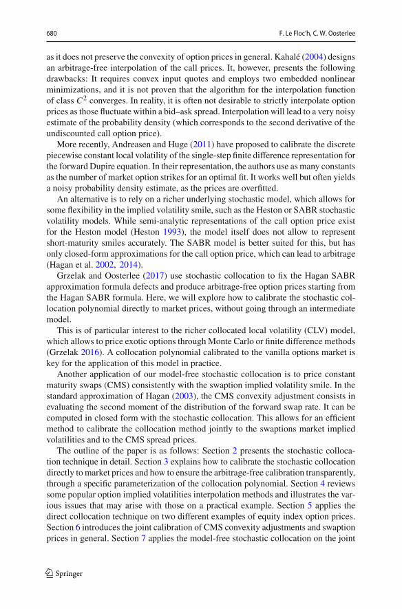
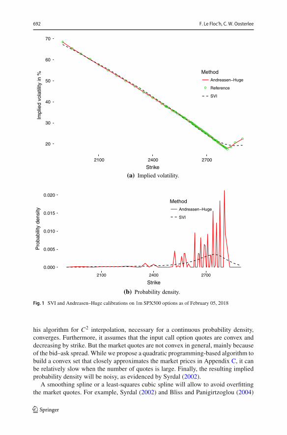
with flat extrapolation. Smoothing is ensured by adding a penalty multiplied by theintegral of the second derivative of the spline function to the objective function. Thesmoothing parameter is challenging to pick. In fact, Syrdal reverts to a manual ad hocchoice of this parameter. Furthermore, the interpolation is a priori not arbitrage-free. Inorder to make it arbitrage-free, an additional nonlinear penalty term against butterflyspread arbitrages needs to be added to the objective function. Instead of a smoothingparameter, the least-squares spline requires to choose the number of knots and theirlocations, which can also seem arbitrary. A slightly different approach is taken byWystup (2015, p. 47) for the foreign exchange optionsmarket, where aGaussian kernelsmoother is applied to the market volatilities as a function of the option delta. Thekernel bandwidth is fixed and the number of kernel points (specific deltas) is typicallylower than the number of market option strikes. Wystup recommends to use up to 7kernel points. While a larger number of points leads to a better fit on our example, itmay also lead to a negative density. With the Gaussian kernel smoothing, the shapeof the implied volatility looks unnatural8 around the point of high curvature (Fig. 2a),and the density can become negative (Fig. 2b). It is thus not always arbitrage-free.

In order to guarantee the arbitrage-free property by construction and still staymodel-free, Andreasen and Huge (2011) use a specific one-step implicit finite differencewhere a discrete piecewise constant local volatility function is calibrated against mar-ket prices. While it is simple and fast, it leads to a noisy implied density, even if wereplace the piecewise constant parameters by a cubic spline (Fig. 1b). This is because,by design, similarly to a spline interpolation, the method overfits the quotes as thenumber of parameters is the same as the number of market option quotes.

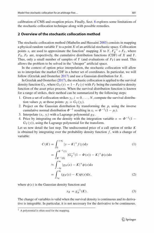
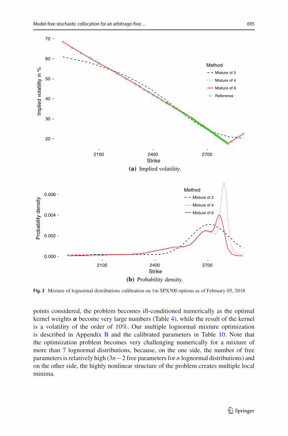
Finally, we can model directly the risk-neutral probability density (RND). Manypapers use the double lognormal mixture of Bahra (Bahra 2007; Arneric et al. 2015)to represent the RND. The double lognormal mixture is not flexible enough to captureour example of short-maturity smile (Fig. 3a). This is extended in Cheng (2010) to amixture of multiple lognormal distributions. With a mixture of 6 lognormal distribu-tions, the root-mean-square error of the model volatilities against market volatilitiesis nearly as low as with Andreasen–Huge (Table 2), and the RND is very smooth.Furthermore, the model is also fully arbitrage-free by construction. But, in similarfashion as the Gaussian kernel smoother (Wystup 2015), the mixture of lognormaldistributions tends to create artificial peaks in the RND (Figs. 2b, 3b), just to fit theinput quotes better on our example.

Compared to theGaussian kernel smoothing, themixture of lognormal distributionsresults in fewer peaks as the volatility of eachdistribution is optimized, but there are stillclearly multiple modes in the density. In reality, as we will see with the collocationmethod, the density has no particular reasons to have multiple modes. Mixture ofnormal or lognormal distributions will, by their nature, tend to create multimodaldensities.

7 Especially for options on a foreign exchange rate, the implied volatilitymay be parameterized as a functionof the option delta, instead of the option strike. Note that the delta is itself a function of the implied volatility,see Appendix A.8 This could be remedied by a kernel smoothing on the strikes instead of the deltas, but then the probabilitydensity goes negative in more places. We thus preferred to stay close to Wystup’s original idea.

123


20

30

40

50

60

70

2100 2400 2700

Strike

Impl

ied

vola

tility

in %

Method

12 points

7 points

Reference


−0.005

0.000

0.005

0.010

0.015

0.020

2100 2400 2700

Strike

Pro

babi

lity

dens

ity Method

12 points

7 points


Fig. 2 Gaussian kernel smoothing calibrations on 1m SPX500 options as of February 05, 2018

Let us give more details about the setup of each technique on our example. Forthe SVI parameterization, we use the quasi-explicit calibration method described inZeliade Systems (2009), which leads to the parameters of Table 3. For the Andreasen–Huge method, we use a dense log-uniform grid composed of 800 points and solvethe probability density (the Fokker–Planck equation) instead of the call prices. Wethen interpolate in between grid points by integrating the density to obtain the calloption prices to preserve the arbitrage-free property everywhere in a similar spirit as(Hagan et al. 2014; Le Floc’h and Kennedy 2017).Weminimize the error measureMV

with the Levenberg–Marquardt algorithm. The Gaussian kernel smoother calibrationis described in Appendix A. We use, respectively, 7 and 12 kernel points, with abandwidth of 0.5 and 0.3. When the bandwidth is too large for the number of kernel

123


20

30

40

50

60

70

2100 2400 2700Strike

Impl

ied

vola

tility

in %

Method

Mixture of 2

Mixture of 4

Mixture of 6

Reference


0.000

0.002

0.004

0.006

2100 2400 2700Strike

Pro

babi

lity

dens

ity

Method

Mixture of 2

Mixture of 4

Mixture of 6


Fig. 3 Mixture of lognormal distributions calibration on 1m SPX500 options as of February 05, 2018

points considered, the problem becomes ill-conditioned numerically as the optimalkernel weights α become very large numbers (Table 4), while the result of the kernelis a volatility of the order of 10%. Our multiple lognormal mixture optimizationis described in Appendix B and the calibrated parameters in Table 10. Note thatthe optimization problem becomes very challenging numerically for a mixture ofmore than 7 lognormal distributions, because, on the one side, the number of freeparameters is relatively high (3n−2 free parameters for n lognormal distributions) andon the other side, the highly nonlinear structure of the problem creates multiple localminima.

123


Table 2 Root-mean-square error(RMSE) of the calibrated modelvolatilities against the marketvolatilities

Model Free parameters RMSE

SVI 5 0.00757

Andreasen–Huge 75 0.00088

Gaussian smoothing kernel 7 0.00400

Gaussian smoothing kernel 12 0.00175

Mixture of 2 lognormals 4 0.01807



Table 3 Parameters resulting of the calibration of the SVI model σ 2(k) = a + b {ρ(k − m)

+√

(k − m)2 + s2}against 1m SPX500 options as of February 05, 2018, with k = ln K

F

a b ρ s m

0.000 0.794 −0.492 0.0537 0.0554

Table 4 Optimal kernelobservations αi resulting of theGaussian kernel smoothingagainst 1m SPX500 options asof February 05, 2018, fordifferent bandwidths λ

Number of points λ min |αi | max |αi |7 0.5 4.8E03 1.1E05

12 0.292 2.5E05 1.3E08

12 0.5 1.6E10 1.2E13

5 Polynomial collocation of SPX500 options

Previous literature has explored the calibration of stochastic collocation againstmarketquotes for interest rates swaptions, in the case of the SABR model in Grzelak andOosterlee (2017) as well as for FX options. In both cases, the set of quotes is relativelysmall (usually less than 10) and the risk of arbitrage in the quotes, related to the bid–ask spread size, is very low. In the world of equity options, the quotes are denser (it isnot unusual to have 50 quotes for liquid equity indices), or less liquid, and thus havea higher probability of containing small theoretical arbitrages.

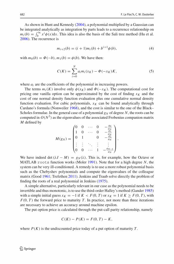
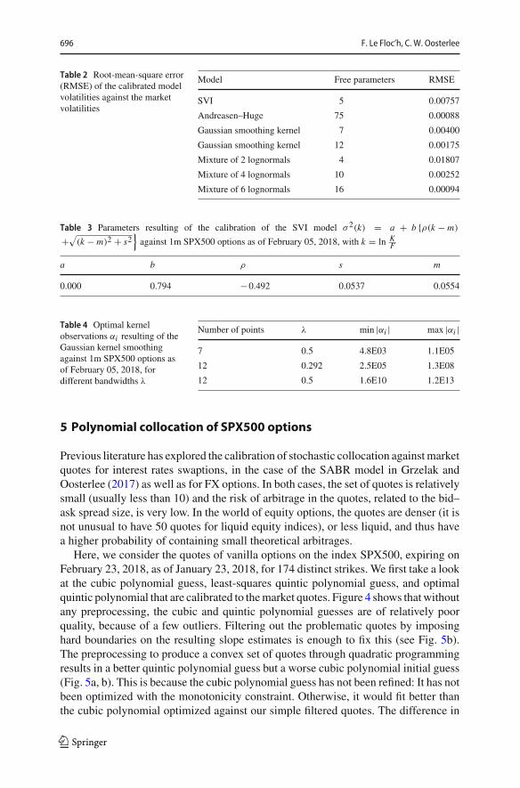
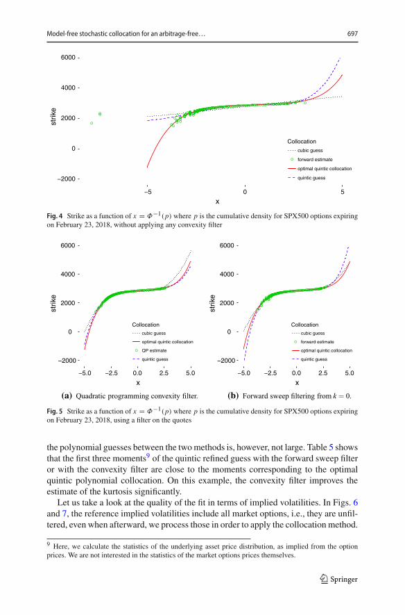
Here, we consider the quotes of vanilla options on the index SPX500, expiring onFebruary 23, 2018, as of January 23, 2018, for 174 distinct strikes. We first take a lookat the cubic polynomial guess, least-squares quintic polynomial guess, and optimalquintic polynomial that are calibrated to themarket quotes. Figure 4 shows thatwithoutany preprocessing, the cubic and quintic polynomial guesses are of relatively poorquality, because of a few outliers. Filtering out the problematic quotes by imposinghard boundaries on the resulting slope estimates is enough to fix this (see Fig. 5b).The preprocessing to produce a convex set of quotes through quadratic programmingresults in a better quintic polynomial guess but a worse cubic polynomial initial guess(Fig. 5a, b). This is because the cubic polynomial guess has not been refined: It has notbeen optimized with the monotonicity constraint. Otherwise, it would fit better thanthe cubic polynomial optimized against our simple filtered quotes. The difference in

123


−2000

0

2000

4000

6000

−5 0 5

x

strik

e

Collocation

cubic guess

forward estimate

optimal quintic collocation

quintic guess

Fig. 4 Strike as a function of x = Φ−1(p) where p is the cumulative density for SPX500 options expiringon February 23, 2018, without applying any convexity filter

−2000

0

2000

4000

6000

x

strik

e

Collocation

cubic guess


QP estimate

quintic guess

(a) Quadratic programming convexity filter.

−2000

0

2000

4000

6000

−5.0 −2.5 0.0 2.5 5.0 −5.0 −2.5 0.0 2.5 5.0

x

strik

e

Collocation

cubic guess

forward estimate


quintic guess

(b) Forward sweep filtering from k = 0.

Fig. 5 Strike as a function of x = Φ−1(p) where p is the cumulative density for SPX500 options expiringon February 23, 2018, using a filter on the quotes

the polynomial guesses between the twomethods is, however, not large. Table 5 showsthat the first three moments9 of the quintic refined guess with the forward sweep filteror with the convexity filter are close to the moments corresponding to the optimalquintic polynomial collocation. On this example, the convexity filter improves theestimate of the kurtosis significantly.

Let us take a look at the quality of the fit in terms of implied volatilities. In Figs. 6and 7, the reference implied volatilities include all market options, i.e., they are unfil-tered, even when afterward, we process those in order to apply the collocation method.

9 Here, we calculate the statistics of the underlying asset price distribution, as implied from the optionprices. We are not interested in the statistics of the market options prices themselves.

123


Table 5 Mean, variance, skew and kurtosis corresponding to quintic polynomial collocation of SPX5001m options as of February 5, 2018, for different filtering of market quotes

Collocation polynomial Mean Variance Skew Kurtosis

Refined quintic guess on raw quotes 2839.00 102.59 −1.59 14.72

Refined quintic guess with forward sweep 2839.00 93.36 −2.74 58.97

Refined quintic guess on convex quotes 2839.00 88.06 −2.63 38.87

Optimal quintic polynomial collocation 2839.00 88.92 −2.71 38.52

20

40

60

1500 2000 2500 3000Strike

Impl

ied

vola

tility

in % Method

Cubic collocation

Quintic collocation

Reference

SVI

Fig. 6 SPX500 smile

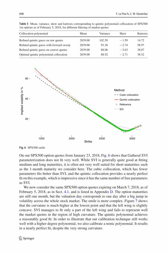
On our SPX500 option quotes from January 23, 2018, Fig. 6 shows that Gatheral SVIparameterization does not fit very well. While SVI is generally quite good at fittingmedium and long maturities, it is often not very well suited for short maturities suchas the 1-month maturity we consider here. The cubic collocation, which has fewerparameters fits better than SVI, and the quintic collocation provides a nearly perfectfit on this example, which is impressive since it has the same number of free parametersas SVI.

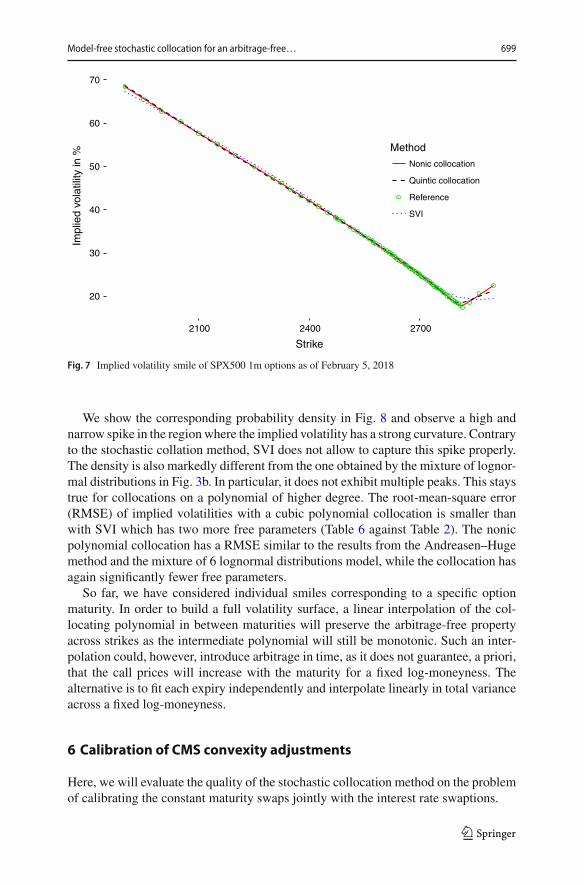
We now consider the same SPX500 option quotes expiring on March 7, 2018, as ofFebruary 5, 2018, as in Sect. 4.1, and is listed in Appendix D. The option maturitiesare still one month, but the valuation day corresponds to one day after a big jump involatility across the whole stock market. The smile is more complex. Figure 7 showsthat the curvature is much higher at the lowest point and that the left wing is slightlyconcave. SVI manages to fit only a part of the left wing and fails to represent wellthe market quotes in the region of high curvature. The quintic polynomial achievesa reasonably good fit. In order to illustrate that our calibration technique still workswell with a higher degree polynomial, we also calibrate a nonic polynomial. It resultsin a nearly perfect fit, despite the very strong curvature.

123


20

30

40

50

60

70

2100 2400 2700

Strike

Impl

ied

vola

tility

in %

Method

Nonic collocation

Quintic collocation

Reference

SVI

Fig. 7 Implied volatility smile of SPX500 1m options as of February 5, 2018

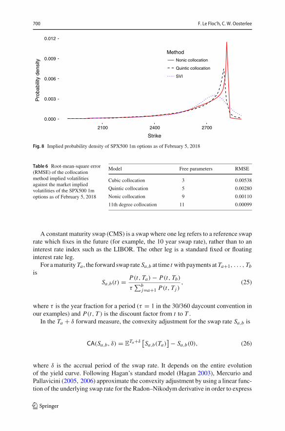
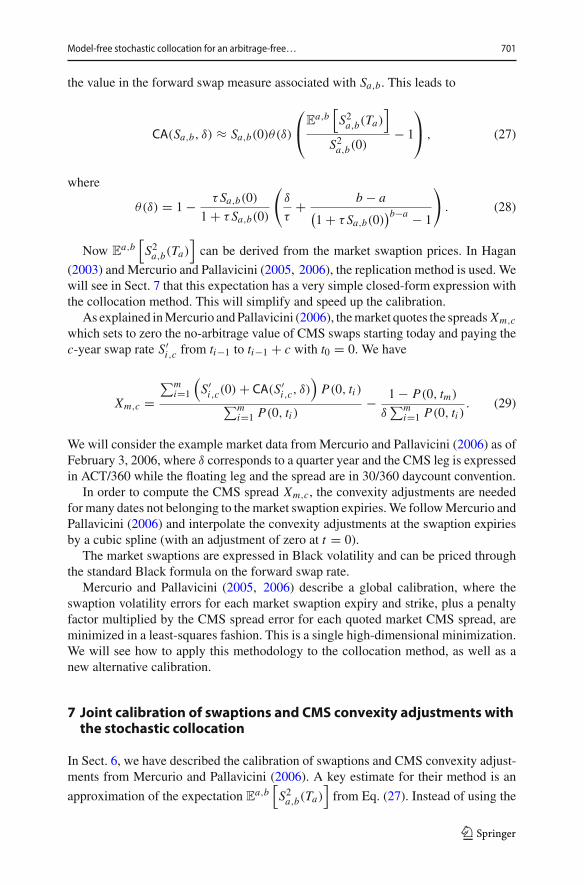
We show the corresponding probability density in Fig. 8 and observe a high andnarrow spike in the regionwhere the implied volatility has a strong curvature. Contraryto the stochastic collation method, SVI does not allow to capture this spike properly.The density is also markedly different from the one obtained by the mixture of lognor-mal distributions in Fig. 3b. In particular, it does not exhibit multiple peaks. This staystrue for collocations on a polynomial of higher degree. The root-mean-square error(RMSE) of implied volatilities with a cubic polynomial collocation is smaller thanwith SVI which has two more free parameters (Table 6 against Table 2). The nonicpolynomial collocation has a RMSE similar to the results from the Andreasen–Hugemethod and the mixture of 6 lognormal distributions model, while the collocation hasagain significantly fewer free parameters.

So far, we have considered individual smiles corresponding to a specific optionmaturity. In order to build a full volatility surface, a linear interpolation of the col-locating polynomial in between maturities will preserve the arbitrage-free propertyacross strikes as the intermediate polynomial will still be monotonic. Such an inter-polation could, however, introduce arbitrage in time, as it does not guarantee, a priori,that the call prices will increase with the maturity for a fixed log-moneyness. Thealternative is to fit each expiry independently and interpolate linearly in total varianceacross a fixed log-moneyness.

6 Calibration of CMS convexity adjustments

Here, we will evaluate the quality of the stochastic collocation method on the problemof calibrating the constant maturity swaps jointly with the interest rate swaptions.

123


0.000

0.003

0.006

0.009

0.012

2100 2400 2700

Strike

Pro

babi

lity

dens

ity

Method

Nonic collocation

Quintic collocation

SVI

Fig. 8 Implied probability density of SPX500 1m options as of February 5, 2018

Table 6 Root-mean-square error(RMSE) of the collocationmethod implied volatilitiesagainst the market impliedvolatilities of the SPX500 1moptions as of February 5, 2018

Model Free parameters RMSE

Cubic collocation 3 0.00538

Quintic collocation 5 0.00280

Nonic collocation 9 0.00110

11th degree collocation 11 0.00099

A constant maturity swap (CMS) is a swap where one leg refers to a reference swaprate which fixes in the future (for example, the 10 year swap rate), rather than to aninterest rate index such as the LIBOR. The other leg is a standard fixed or floatinginterest rate leg.

For amaturity Ta , the forward swap rate Sa,b at time t with payments at Ta+1, . . . , Tbis

Sa,b(t) = P(t, Ta) − P(t, Tb)

τ∑b

j=a+1 P(t, Tj ), (25)

where τ is the year fraction for a period (τ = 1 in the 30/360 daycount convention inour examples) and P(t, T ) is the discount factor from t to T .

In the Ta + δ forward measure, the convexity adjustment for the swap rate Sa,b is

CA(Sa,b, δ) = ETa+δ

[Sa,b(Ta)

] − Sa,b(0), (26)

where δ is the accrual period of the swap rate. It depends on the entire evolutionof the yield curve. Following Hagan’s standard model (Hagan 2003), Mercurio andPallavicini (2005, 2006) approximate the convexity adjustment by using a linear func-tion of the underlying swap rate for the Radon–Nikodym derivative in order to express

123


the value in the forward swap measure associated with Sa,b. This leads to

CA(Sa,b, δ) ≈ Sa,b(0)θ(δ)

⎛⎝E

a,b[S2a,b(Ta)

]

S2a,b(0)− 1

⎞⎠ , (27)

where

θ(δ) = 1 − τ Sa,b(0)

1 + τ Sa,b(0)

(δ

τ+ b − a(

1 + τ Sa,b(0))b−a − 1

). (28)

Now Ea,b

[S2a,b(Ta)

]can be derived from the market swaption prices. In Hagan

(2003) and Mercurio and Pallavicini (2005, 2006), the replication method is used. Wewill see in Sect. 7 that this expectation has a very simple closed-form expression withthe collocation method. This will simplify and speed up the calibration.

As explained inMercurio andPallavicini (2006), themarket quotes the spreads Xm,c

which sets to zero the no-arbitrage value of CMS swaps starting today and paying thec-year swap rate S′

i,c from ti−1 to ti−1 + c with t0 = 0. We have

Xm,c =∑m

i=1

(S′i,c(0) + CA(S′

i,c, δ))P(0, ti )∑m

i=1 P(0, ti )− 1 − P(0, tm)

δ∑m

i=1 P(0, ti ). (29)

We will consider the example market data fromMercurio and Pallavicini (2006) as ofFebruary 3, 2006, where δ corresponds to a quarter year and the CMS leg is expressedin ACT/360 while the floating leg and the spread are in 30/360 daycount convention.

In order to compute the CMS spread Xm,c, the convexity adjustments are neededfor many dates not belonging to themarket swaption expiries.We followMercurio andPallavicini (2006) and interpolate the convexity adjustments at the swaption expiriesby a cubic spline (with an adjustment of zero at t = 0).

The market swaptions are expressed in Black volatility and can be priced throughthe standard Black formula on the forward swap rate.

Mercurio and Pallavicini (2005, 2006) describe a global calibration, where theswaption volatility errors for each market swaption expiry and strike, plus a penaltyfactor multiplied by the CMS spread error for each quoted market CMS spread, areminimized in a least-squares fashion. This is a single high-dimensional minimization.We will see how to apply this methodology to the collocation method, as well as anew alternative calibration.

7 Joint calibration of swaptions and CMS convexity adjustments withthe stochastic collocation

In Sect. 6, we have described the calibration of swaptions and CMS convexity adjust-ments from Mercurio and Pallavicini (2006). A key estimate for their method is an

approximation of the expectation Ea,b

[S2a,b(Ta)

]from Eq. (27). Instead of using the

123


replicationmethod,when a collocation polynomial is calibrated to themarket swaptionprices, this expectation can be computed by a direct integration:

Ea,b

[S2a,b(Ta)

]=

∫ ∞

−∞g2N (x)φ(x)dx . (30)

The coefficients (b0, . . . , b2N ) of g2N correspond to the self-convolution of the coef-ficients (a0, . . . , aN ) of gN . Similarly to the calculation of the first moment, therecurrence relation [Eq. (4)] leads to the closed-form expression

Ea,b

[S2a,b(Ta)

]= b0 +

N∑i=1

(2i − 1)!!b2i . (31)

There are two ways to include the CMS spread in the calibration of the smile to theswaption quotes, which we will label as the global and the decoupled approach. Thecollocation method can be used in the global approach from Mercurio and Pallavicini(2006), by first computing an initial guess in the form of a list of isotonic representa-tions, out-of-the-market swaption quotes for each expiry according to Sect. 3. Then,the least-squares minimization updates the isotonic representations iteratively.

Tables 7 and 8 show that the error with a quintic collocation polynomial is as lowas with the SABR interpolation.10 Compared to SABR interpolation, however, theadvantages of stochastic collocation are: it is arbitrage-free by construction, while theSABR approximation formula has known issues with low or negative rates (Haganet al. 2014); the accuracy of the fit can be improved by simply increasing the collocatingpolynomial degree; the calculation of the CMS convexity adjustment is much fasteras it does not involve an explicit replication.

The decoupled calibration procedure consists of the following two steps:

(A) Find the optimal convexity adjustment for each market swaption expiry

– Compute the initial guess for each convexity adjustment by fitting the swaptionsmile at each expiry as described in Sect. 3, without taking into account anyCMS spread price.

– Compute the cubic spline which interpolates the convexity adjustments acrossthe expiries. Minimize the square root of CMS spread errors, by adjusting theconvexity adjustments and recomputing the cubic spline, for example, with theLevenberg–Marquardt algorithm.

(B) Minimize the square of the swaption volatility error plus a penalty factormultiplied by the convexity adjustment error, against the optimal convexityadjustment for each expiry independently.

The penalty factor allows to balance the swaption volatilities fit with the CMS spreadfit. The decoupled calibration involves n+1 independent low-dimensional minimiza-tions, with n being the number of swaptions expiries.

10 The SABR numbers come from Mercurio and Pallavicini (2006). For the Black model, our numbersdiffer slightly from Mercurio and Pallavicini, likely because of the handling of holidays.

123


Table 7 Absolute differences (in bp) between market and model swaptions implied volatilities

Strike −200 −100 −50 −25 0 25 50 100 200

SABR

5 × 10 1.1 0.2 0.3 0.5 0.2 0.2 0.8 0.2 0.4

10 × 10 0.2 0.1 0.4 0.3 0.1 0.2 0.4 0.5 0.3

20 × 10 0.8 0.6 0.4 0.4 0 0.3 0.3 0.5 0.5

Quintic global

5 × 10 0.1 − 0.4 0.3 0.4 0.2 − 0.5 − 0.3 0.3 0.0

10 × 10 0.4 − 1.8 0.4 1.0 1.3 0.2 − 0.5 − 1.7 1.0

20 × 10 0.7 − 1.7 0.8 1.2 1.1 0.5 − 0.7 − 1.8 1.3

Quintic decoupled

5 × 10 0.0 − 0.3 0.2 0.3 0.2 − 0.5 − 0.3 0.4 − 0.1

10 × 10 0.1 − 0.6 0.2 0.3 0.6 − 0.2 − 0.3 − 0.4 0.3

20 × 10 0.4 − 2.0 0.6 1.0 1.0 0.5 − 0.6 − 1.6 0.9

Strikes are expressed as absolute differences in basis points w.r.t the at-the-money values

Table 8 Absolute differences (in bp) between market CMS swap spreads and those induced by the SABRfunctional form, the Black model and the collocation of a quintic polynomial for the 10-year tenor

Maturity (years) SABR Black Quintic global Quintic decoupled

5 0.8 0.0 0.3 0.3

10 1.7 2.3 1.2 1.4

15 1.8 3.2 1.3 1.7

20 1.3 4.0 1.3 1.8

30 2.1 6.3 2.3 1.9

Table 9 CMS convexity adjustments (in bp) for different expiries for the 10-year tenor

Expiry 1years 5years 10years 20years 30years

Optimal CA (step A) 1.75 10.62 20.24 35.02 49.41

Decoupled CA (step B) 1.75 10.63 20.52 37.14 60.41

Table 9 presents the optimal convexity adjustments for CMS swaps of tenor 10yearsusing the market data of Mercurio and Pallavicini resulting from the first step of thedecoupled calibration method. With a cubic spline interpolation on these adjustments,the error in market CMS spreads is then essentially zero. The adjustments resultingfrom the second step are also displayed for indication.

As evidenced in Tables 7 and 8, the error in the swaptions volatilities and in theCMS spreads is as small as, or smaller than the decoupled calibration when comparedto the global calibration. In Fig. 9, we look at the smile generated by the quinticcollocation calibrated with a penalty of 1 (which corresponds to a balanced fit of

123


15

20

−200 0 200 400Strike

Vol

atili

ty

Calibration step

Reference

Step A, penalty=10000

Step B, penalty=1

Fig. 9 20× 10 swaption smile, calibrated with a penalty factor of 10,000 (exact CMS spread prices) and apenalty factor of 1 (balanced fit corresponding to Table 8)

market CMS spreads vs. swaption volatilities as in Table 8) and a penalty of 10,000(which corresponds to a nearly exact fit to the CMS spreads).

Instead of using a monotonic quintic polynomial, we could have used a monotoniccubic polynomial with quadratic left and right C1-extrapolation. Two parameters ofeach extrapolation would be set by the value and slope continuity conditions, and theremaining extra parameter could be used to calibrate the tail against the CMS prices.Overall, it would involve the same number of parameters to calibrate and would likelybe more flexible. The calibration technique would, however, remain the same: Allthe parameters would need to be recalibrated as changes in the extrapolation result inchanges in the first two moments of the distribution as well.

8 Limitations of the stochastic collocation

A question which remains is whether the stochastic collocation method can also fitmultimodal distributions well?

Theorem 1 For any continuous survival distribution function GY , there exists astochastic collocation polynomial gN which can approximate the survival distributionto any given accuracy ε > 0 across an interval [a, b] of R.Proof The function g(x) = G−1

Y (1 − Φ(x)) is continuous andmonotone onR.Wolib-ner (1951) and Lorentz and Zeller (1968) have shown that for any η > 0, there exists amonotone polynomial gN ,η such that supx∈[a,b]

∥∥g(x) − gN ,η(x)∥∥ ≤ η on any interval

[a, b] of R. From Eq. (2), the approximate survival distribution corresponding to the

123


collocation polynomial gN ,η is GN ,η = 1− Φ ◦ g−1N ,η where the symbol ◦ denotes the

function composition.Let I = [gN ,η(a), gN ,η(b)], Φ ◦ g−1

N ,η and thus GN ,η are also monotone and con-

tinuous on I . Let J = [1−Φ(b), 1−Φ(a)], and hN ,η = gN ,η ◦Φ−1 ◦ (1− id) whereid is the identity function. We have G−1

Y = g ◦ Φ−1 ◦ (1− id). As Φ−1 ◦ (1− id) iscontinuous and monotone, we have

supy∈J

∥∥∥G−1Y (y) − hN ,η(y)

∥∥∥ ≤ η.

As h−1N is continuous and monotone on I , we also have

supx∈I

∥∥∥G−1Y ◦ h−1

N ,η(x) − x∥∥∥ ≤ η. (32)

The uniform continuity of GY implies that for each ε > 0, we can find an η > 0 suchthat, if Eq. (32) holds, then

supx∈I

∥∥∥h−1N ,η(x) − GY (x)

∥∥∥ ≤ ε.

In reality, simple multimodal distributions can be challenging to approximate in

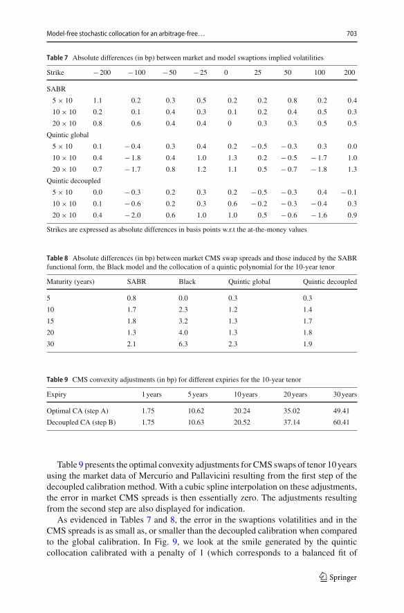
practice, as they might require a very high degree of the collocation polynomial foran accurate representation. In order to illustrate this, we consider an equally weightedmixture of two Gaussian distributions of standard deviation 0.1 centered, respectively,at f1 = 0.8 and f2 = 1.2. We can price vanilla options based on this density, simplyby summing the prices of two options using a forward at, respectively, f1 and f2under the Bachelier model. We set the forward F(0, T ) = 1 and consider 20 optionsof maturity T = 1 and equidistant strikes between 0.5 and 1.5.

The Black volatility smile implied by this model is absolutely not realistic (Fig. 10),but it is perfectly valid and arbitrage-free theoretically, and we can still calibrate ourmodels to it.

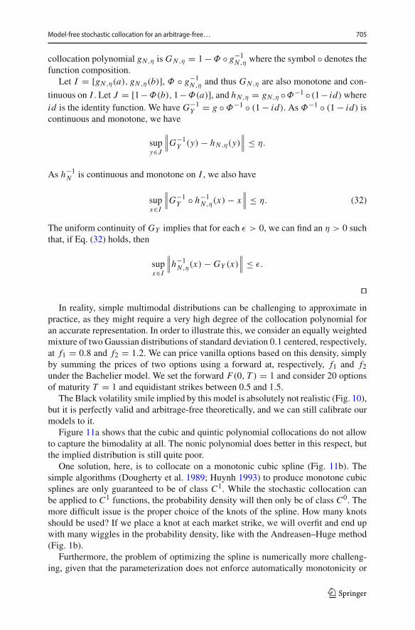
Figure 11a shows that the cubic and quintic polynomial collocations do not allowto capture the bimodality at all. The nonic polynomial does better in this respect, butthe implied distribution is still quite poor.

One solution, here, is to collocate on a monotonic cubic spline (Fig. 11b). Thesimple algorithms (Dougherty et al. 1989; Huynh 1993) to produce monotone cubicsplines are only guaranteed to be of class C1. While the stochastic collocation canbe applied to C1 functions, the probability density will then only be of class C0. Themore difficult issue is the proper choice of the knots of the spline. How many knotsshould be used? If we place a knot at each market strike, we will overfit and end upwith many wiggles in the probability density, like with the Andreasen–Huge method(Fig. 1b).

Furthermore, the problem of optimizing the spline is numerically more challeng-ing, given that the parameterization does not enforce automatically monotonicity or

123


12

16

20

24

0.50 0.75 1.00 1.25 1.50

Strike

Impl

ied

vola

tility

in %

Method

Kernel

Nonic

Quintic

Fig. 10 Black implied volatility smile for a bimodal distribution and the calibrated stochastic collocationsmiles with a quintic and a nonic polynomial

0

1

2

3

4

5

Strike

Pro

babi

lity

dens

ity Method

Cubic

Kernel

Nonic

Quintic

(a) Polynomial collocation.

0

1

2

3

4

5

0.50 0.75 1.00 1.25 1.50 0.50 0.75 1.00 1.25 1.50

Strike

Pro

babi

lity

dens

ity

Method

Kernel

Spline

(b) Spline collocation.

Fig. 11 Probability density obtained by the stochastic collocation of a reference bimodal distribution

martingality. Regardingmonotonicity, in the case of the algorithm fromHyman (1983)or Dougherty et al. (1989), a nonlinear filter is applied, which could make the opti-mizer get stuck in a local minimum. Finally, there is the issue of which boundaryconditions and which extrapolation to choose. A linear extrapolation, combined withthe so-called natural boundary conditions, would result in a smooth density,11 but thelinear extrapolation still has to be of positive slope in order to guarantee the mono-tonicity overR. A priori, this is not guaranteed. An alternative is to rely on the forward

11 Although this makes the model relatively rigid toward the wings representation.

123


difference estimate as the slope, along with clamped boundary conditions, at the costof losing the continuity of the probability density at the boundaries.

9 Conclusion

We have shown how to apply the stochastic collocation method directly to marketoptions quotes in order to produce a smooth and accurate interpolation and extrapo-lation of the option prices, even on challenging equity options examples. A specificisotonic parameterization was used to ensure the monotonicity of the collocation poly-nomial as well as the conservation of the zeroth and first moments transparently duringthe optimization, guaranteeing the absence of arbitrages.

The polynomial stochastic collocation leads to a smooth implied probability density,without any artificial peak, even with high degrees of the collocation polynomial. Wealso applied the technique to interest rate derivatives. This results in closed-formformula for CMS convexity adjustments, which can thus be easily calibrated jointlywith interest rate swaptions.

Finally, we illustrated, on a theoretical example, how the polynomial stochasticcollocation had difficulties in capturing multimodal distributions.

Open Access This article is distributed under the terms of the Creative Commons Attribution 4.0 Interna-tional License (http://creativecommons.org/licenses/by/4.0/), which permits unrestricted use, distribution,and reproduction in any medium, provided you give appropriate credit to the original author(s) and thesource, provide a link to the Creative Commons license, and indicate if changes were made.

A Gaussian kernel smoothing

Let (xi , yi )i=0,...,m be m + 1 given points. Using the points (xk)k=0,...,n , which aretypically within the interval (x0, xm), a smooth interpolation is given by the functiong defined by

g(x) = 1∑nk=0 ψλ(x − xk)

n∑k=0

αkψλ(x − xk) (33)

for x ∈ R, n ≤ m and where ψλ is the kernel. The Gaussian kernel is defined by

ψλ(u) = 1

λ√2π

e− u2

2λ2 . (34)

The calibration consists in finding the αi that minimizes the given error measure on theinput (xi , yi )i=0,...,m . The solution can be found by QR decomposition of the linearproblem

⎛⎜⎝

ψλ(x0 − x0) ψλ(x0 − x1) . . . ψλ(x0 − xn)...

... . . ....

ψλ(xm − x0) ψλ(xm − x1) . . . ψλ(xm − xn)

⎞⎟⎠

⎛⎜⎝

α0...

αn

⎞⎟⎠

123

http://creativecommons.org/licenses/by/4.0/


=⎛⎜⎝

y0∑n

k=0ψλ(x0 − xk)...

ym∑n

k=0ψλ(xm − xk)

⎞⎟⎠ . (35)

The xi are typically option strikes, log-moneynesses or deltas. The yi are the cor-responding option implied volatilities. Wystup (2015) applies the method in terms ofoption deltas. There are multiple delta definitions in the context of volatility interpo-lation; we use the undiscounted call option forward delta:

� = Φ

(1

σ√Tln

F(0, T )

K+ 1

2σ√T

)(36)

where Φ is the cumulative normal distribution function, F(0, T ) is the forward tomaturity T , K is the option strike and σ is the corresponding option volatility.

When thepoints are defined in delta,weneed tofind thedelta for a givenoption strikein order to compute the option implied volatility or the option price for a given strike.But the delta is also a function of the implied volatility. This is a nonlinear problem.Equation 36,withσ = g(�), is solved by a numerical solver such as Toms348 (Alefeldet al. 1995) or a simple bisection, starting at � = 0.5, in the interval [0, 1].

Wystup recommends a bandwidth of 0.25;wefind that a bandwidth of 0.5minimizesthe root-mean-square error of implied volatilities on our example.

B Mixture of lognormal distributions

Let (xi , yi )i=0,...,m be m + 1 given points. Using the points (xk)k=0,...,n , which aretypically within the interval (x0, xm), a kernel estimate of the density on the points xkis

g(x) =n∑

k=0

αkψλk (x, xk), (37)

where ψλk is a kernel of bandwidth λk , along with the condition∑n

k=0 αk = 1 andαk ≥ 0 for k = 0, . . . , n.

In our case, (yi )i=0,...,m are option prices, and we want to estimate the underlyingdistribution.We then consider thatψλk (x) is a Gaussian and x is a logarithmic functionof the option strike K , x = ln(K ). In order to map the kernel exactly to the Black–Scholes probability density, we use

ψλk (x, xk) = 1

λk√2π

e−

(x−xk+ 1

2 λ2k

)22λ2k

−xk. (38)

The option price of strike K = ex is then given by

V (x) =n∑

k=0

αkVBlack(ex , exk , λk, 1), (39)

123


where VBlack(K , f , λ, T ) is the price of a vanilla option of maturity T and strike Kgiven by the Black-76 formula for an asset of forward f and volatility λ.

The calibration consists then finding the parameters αk, xk, λk that minimize themeasure MV . In the calibration, we will also add the martingality constraint, whichwill ensure that the put-call parity holds exactly in the mixture model. This translatesto the additional constraint

n∑k=0

αkexk = F(0, T ), (40)

where F(0, T ) is the underlying asset forward to maturity.We can enforce the constraints by a variable transformation. The

√αk are located

on the hypersphere of radius R = 1 in Rn+1. Let θ ∈ R

n , a point u ∈ Rn+1 is on the

hypersphere if and only if

uk = R cos(θk)k−1∏j=0

sin(θ j ) (41)

for k = 0, . . . , n − 1 and un = ∏nj=0 sin(θ j ). We thus use the transform αk = u2k . It

is invertible and the inverse is

θk = π

2− arctan

⎛⎝ uk√∑n

j=k+1 u2j

⎞⎠ , (42)

or directly in terms of αk :

θk = π

2− arctan

(√αk∑n

j=k+1 α j

). (43)

The martingality condition can be enforced the same way, using the intermediatevariable zk = αkexk . Indeed, Eq. (40) means that zk is located on the hypersphere ofradius R = √

F(0, T ) in Rn+1.This allows the use of an unconstrained algorithm such as Levenberg–Marquardt

to minimize the error measure MV on R3n+1. As an initial guess, we use αk = 1

n+1 ,

xk = F(0, T ), λk = σATM√T where σATM is the implied volatility of the option whose

strike is closest to the forward price.If negative strikes are allowed, we can replace lognormal distributions by nor-

mal distributions, and the Black–Scholes formula by the Bachelier one. Note that ifthe bandwidth (λk) and the mean (xk) are fixed in advance, the problem becomes aquadratic programming problem (Table 10).

123


Table 10 Calibrated mixture of lognormal distributions against 1m SPX500 options as of February 05,2018, for different number of distributions

Mixture of 2 lognormals

α 0.1664 0.8336

ex 2208.46 2713.91

λ 0.1561 0.04033


α 0.09789 0.2739 0.3489 0.2793

ex 2203.35 2523.00 2701.93 2793.91

λ 0.2467 0.06519 0.02442 0.006543


α 0.02164 0.1121 0.2480 0.2593 0.1794 0.1795

ex 2045.69 2242.37 2551.67 2696.07 2812.76 2771.53

λ 0.5711 0.1129 0.04712 0.01909 1.576e−05 0.008333

C An algorithm to build a good convex set from themarket calloption prices

Let (yi )i=0,...,m be the market option strikes and (ci )i=0,...,m the corresponding calloption prices. Boyd and Vandenberghe (2004, p. 338) show that the least-squaresconvex piecewise-linear function f (y) = maxi=0,...,m ci−gi (y−yi )fitting the (yi , ci )is the solution of a quadratic programming problem:

minimizem∑i=0

(ci − ci )2

subject to ci + gi (y j − yi ) ≤ c j , i, j = 0, . . . ,m,

and − 1 + ε < gi < −ε, i = 0, . . . ,m.

where ci , gi are 2(m + 1) free parameters. The constraints on gi make sure thatour piecewise-linear function respects the call prices no-arbitrage bounds. Most ofthose constraints are redundant with the convexity constraints: they can be reducedto −1 + ε < g0 and gm < −ε. A robust quadratic solver such as CVXOPT can beused, and we have then a good initial convex estimate of the call prices by evaluatingthis piecewise-linear function at each market strike. The estimate is thus given by(yi , ci )i=0,...,m .

For 75 option quotes, the constraints consist in a sparsematrix of 5775 rows and 150columns. The python implementation of CVXOPT takes 0.38 s to solve the quadraticprogramming problem on an Intel Core i7 7700U processor.

123


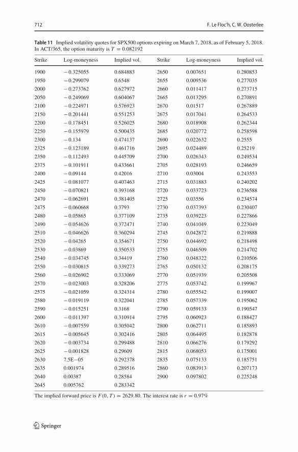
D Implied volatility quotes for vanilla options on SPX500 expiring onMarch 7, 2018, as of February 5, 2018

The implied volatilities were obtained by using the mid-price of call and put options.The forward price is implied from the put-call parity relationship (Table 11).

E Example code

The following Matlab/Octave code will calibrate the collocated polynomial to marketimplied volatilities, without any filtering of the market quotes. The code is meant onlyas an illustration of the method and is not particularly robust or fast.

Listing 1 makeIsotonicCollocation.m - Matlab/Octave code to compute the optimal collocation polynomialfor a given set of option strikes and vols.

function C = makeIsotonicCollocation(strikes , vols , tte , forward , degree)m = length(strikes);[prices , vegas] = blackCall(strikes , forward , vols , tte);dx = diff(strikes ,1); dz = diff(prices ,1)./dx;s = (dx(1:m-2) .* dz(2:m-1) + dx(2:m-1) .* dz(1:m-2)) ./ (dx(1:m-2)+dx(2:m-1));x = -stdnormal_inv(-s);binfilter = !isnan(x); x = x(binfilter); y = strikes (2:m-1)(binfilter);cubic = polyfit(x,y,3); cubic (4)=forward -cubic (2);if cubic (2)^2 - 3* cubic (3)*cubic (1) >= 0

M = [1, 0, 0; 0, sum(x.^2), sum(x.^4); 0, sum(x.^4), sum(x.^6)];R = [forward; sum(x.*y); sum(x.^3 .* y)];C = M \ R;cubic = [abs(C(3)), 0, abs(C(2)), forward ];

endC1 = [sqrt (3* cubic (1)), cubic (2)/sqrt (3* cubic (1))];C2 = [sqrt(cubic (3)-cubic (2) ^2/(3* cubic (1)))];C1p = zeros (1,( degree +1) /2); C2p = zeros(1, (degree -1) /2);C1p(length(C1p)-length(C1)+1: length(C1p)) = C1;C2p(length(C2p)-length(C2)+1: length(C2p)) = C2;guess0 = [C1p C2p];guess1 = lsqnonlin(@(guess)isopolyObjective(guess ,x,y,forward ,degree), guess0);weights = min (1.0./ vegas ,1e6/forward);sol = lsqnonlin(@(guess)isocolloObjective(guess1 ,strikes ,prices ,weights ,forward ,degree)

, guess1);[C1 ,C2] = guessToIso(sol ,degree);C = isoToPoly(C1 , C2 , forward);

end

function C = isoToPoly(C1 , C2 , forward)C1sq = conv(C1 ,C1); C2sq = conv(C2 ,C2);sq = zeros(1,length(C1sq));sq(length(C1sq)-length(C2sq)+1: length(C1sq))=C2sq;C = polyint(sq+C1sq);polyForward = polyHermiteIntegral (C);C(length(C)) = forward - polyForward;

end

function [C1 ,C2] = guessToIso(guess ,degree)C1=guess ’(1:( degree +1) /2); C2=guess ’(( degree +1) /2+1: length(guess));

end

function value = isopolyObjective(guess ,x,y,forward , degree)[C1 ,C2] = guessToIso(guess ,degree);C = isoToPoly(C1 ,C2 ,forward);value = polyval(C,x)-y;

end

function value = isocolloObjective(guess ,strikes ,prices ,weights ,forward ,degree)[C1 ,C2] = guessToIso(guess ,degree);C = isoToPoly(C1 ,C2 ,forward);value = (priceEuropeanCall(C, strikes , forward)-prices) .* weights ;

end

function [price , vega] = blackCall(strike , forward , vol , tte)vsqrtt = vol*sqrt(tte);d1 = log(forward ./ strike) ./ vsqrtt + 0.5* vsqrtt; d2 = d1 - vsqrtt;price = forward * stdnormal_cdf(d1) - strike .* stdnormal_cdf(d2);vega = forward*stdnormal_pdf(d1)*sqrt(tte);

end

123


Table 11 Implied volatility quotes for SPX500 options expiring on March 7, 2018, as of February 5, 2018.In ACT/365, the option maturity is T = 0.082192

Strike Log-moneyness Implied vol. Strike Log-moneyness Implied vol.

1900 −0.325055 0.684883 2650 0.007651 0.280853

1950 −0.299079 0.6548 2655 0.009536 0.277035

2000 −0.273762 0.627972 2660 0.011417 0.273715

2050 −0.249069 0.604067 2665 0.013295 0.270891

2100 −0.224971 0.576923 2670 0.01517 0.267889

2150 −0.201441 0.551253 2675 0.017041 0.264533

2200 −0.178451 0.526025 2680 0.018908 0.262344

2250 −0.155979 0.500435 2685 0.020772 0.258598

2300 −0.134 0.474137 2690 0.022632 0.2555

2325 −0.123189 0.461716 2695 0.024489 0.25219

2350 −0.112493 0.445709 2700 0.026343 0.249534

2375 −0.101911 0.433661 2705 0.028193 0.246659

2400 −0.09144 0.42016 2710 0.03004 0.243553

2425 −0.081077 0.407463 2715 0.031883 0.240202

2450 −0.070821 0.393168 2720 0.033723 0.236588

2470 −0.062691 0.381405 2725 0.03556 0.234574

2475 −0.060668 0.3793 2730 0.037393 0.230407

2480 −0.05865 0.377109 2735 0.039223 0.227866

2490 −0.054626 0.372471 2740 0.041049 0.223049

2510 −0.046626 0.360294 2745 0.042872 0.219888

2520 −0.04265 0.354671 2750 0.044692 0.218498

2530 −0.03869 0.350533 2755 0.046509 0.214702

2540 −0.034745 0.34419 2760 0.048322 0.210506

2550 −0.030815 0.339273 2765 0.050132 0.208175

2560 −0.026902 0.333069 2770 0.051939 0.205508

2570 −0.023003 0.328206 2775 0.053742 0.199967

2575 −0.021059 0.324314 2780 0.055542 0.199007

2580 −0.019119 0.322041 2785 0.057339 0.195062

2590 −0.015251 0.3168 2790 0.059133 0.190547

2600 −0.011397 0.310914 2795 0.060923 0.188427

2610 −0.007559 0.305042 2800 0.062711 0.185893

2615 −0.005645 0.302416 2805 0.064495 0.182878

2620 −0.003734 0.299488 2810 0.066276 0.179292

2625 −0.001828 0.29609 2815 0.068053 0.175001

2630 7.5E−05 0.292378 2835 0.075133 0.185751

2635 0.001974 0.289516 2860 0.083913 0.207173

2640 0.00387 0.28584 2900 0.097802 0.225248

2645 0.005762 0.283342

The implied forward price is F(0, T ) = 2629.80. The interest rate is r = 0.97%

123


Listing 2 priceEuropeanCall.m - Matlab/Octave code to price a European call option using a collocationpolynomial for a given set of option strikes.

function value = priceEuropeanCall(C, strike , forward)ck = solveStrike(C,strike);value = polyHermiteIntegralBounded(C,ck) - stdnormal_cdf(-ck).* strike;

end

function ck = solveStrike(C, strike)ck = zeros(1,length(strike));for i=1: length(strike)

Cp = C; Cp(length(Cp)) -= strike(i); Cp /= C(1);r = roots(Cp); r = r(imag(r)==0);ck(i) = r;

endend

function value = polyHermiteIntegral (C)n = length(C); value = C(n); m0=1; m1 = 0;for i=2:(n-1)

m2 = m0 * (i-1); value += C(n-i)*m2; m0=m1; m1=m2;end

end

function value = polyHermiteIntegralBounded(C,x0)n = length(C); m0 = stdnormal_cdf(-x0); nx0 = stdnormal_pdf(x0); m1 = nx0;value = C(n)*m0 + C(n-1)*m1;for i=2:(n-1)

m2 = m0 * (i-1) + nx0 .* (x0 .^ (i-1));value += C(n-i)*m2; m0=m1; m1=m2;

endend

References

Alefeld, G., Potra, F.A., Shi, Y.: Algorithm 748: enclosing zeros of continuous functions. ACMTrans.Math.Softw. (TOMS) 21(3), 327–344 (1995)

Andreasen, J., Huge, B.: Volatility interpolation. Risk 24(3), 76 (2011)Arneric, J., Aljinovic, Z., Poklepovic, T.: Extraction of market expectations from risk-neutral density. J.

Econ. Bus. 33, 235–256 (2015)Bahra, B.: Implied risk-neutral probability density functions from option prices: a central bank perspective.

In: Satchell, S., Knight, J. (eds.) Forecasting Volatility in the Financial Markets, 3rd edn, pp. 201–226.Elsevier, Amsterdam (2007)

Bates, D.S.: Jumps and stochastic volatility: exchange rate processes implicit in Deutsche mark options.Rev. Financ. Stud. 9(1), 69–107 (1996)

Bliss, R.R., Panigirtzoglou, N.: Option-implied risk aversion estimates. J. Finance 59(1), 407–446 (2004)Boyd, S., Vandenberghe, L.: Convex Optimization. Cambridge University Press, Cambridge (2004)Carr, P., Lee, R.: Robust replication of volatility derivatives. Preprint (2008)Carr, P., Stanley, M., Madan, D.: Towards a theory of volatility trading. In: Reprinted in Option Pricing,

InterestRates, andRiskManagement,Musiella, Jouini, Cvitanic, pp. 417–427.University Press (1998)Cheng, M.K.C.: A new framework to estimate the risk-neutral probability density functions embedded in

options prices (10-181) (2010)Christoffersen, P., Heston, S., Jacobs, K.: The shape and term structure of the index option smirk: why

multifactor stochastic volatility models work so well. Manag. Sci. 55(12), 1914–1932 (2009)Dougherty, R.L., Edelman, A.S., Hyman, J.M.: Nonnegativity-, monotonicity-, or convexity-preserving

cubic and quintic hermite interpolation. Math. Comput. 52(186), 471–494 (1989)Dupire, B.: Pricing with a smile. Risk 7(1), 18–20 (1994)Flint, E., Maré, E.: Estimating option-implied distributions in illiquid markets and implementing the ross

recovery theorem. S. Afr. Actuar. J. 17(1), 1–28 (2017)Gander, W.: On Halley’s iteration method. Am. Math. Month. 92, 131–134 (1985)Gatheral, J., Lynch, M.: Lecture 1: Stochastic volatility and local volatility. Case Studies in Financial

Modeling Notes, Courant Institute of Mathematical Sciences (2004)Good, I.: The colleague matrix, a Chebyshev analogue of the companion matrix. Q. J. Math. 12(1), 61–68

(1961)Grzelak, L.A.: The CLV framework—a fresh look at efficient pricing with smile. Browser Download This

Paper (2016)

123


Grzelak, L.A., Oosterlee, C.W.: From arbitrage to arbitrage-free implied volatilities. J. Comput. Finance20(3), 31–49 (2017)

Hagan, P.S.: Convexity conundrums: pricing CMS swaps, caps, and floors. Wilmott 2003(2), 38–45 (2003).https://doi.org/10.1002/wilm.42820030211

Hagan, P.S., Kumar, D., Lesniewski, A.S.,Woodward, D.E.:Managing smile risk.Wilmott magazine (2002)Hagan, P.S., Kumar, D., Lesniewski, A., Woodward, D.: Arbitrage-free SABR. Wilmott 2014(69), 60–75

(2014)Heston, S.L.: A closed-form solution for options with stochastic volatility with applications to bond and

currency options. Rev. Financ. Stud. 6(2), 327–343 (1993)Hu, Z., Kerkhof, J., McCloud, P., Wackertapp, J.: Cutting edges using domain integration. Risk 19(11), 95

(2006)Hunt, P., Kennedy, J.: Financial Derivatives in Theory and Practice. Wiley, New York (2004)Huynh, H.T.: Accurate monotone cubic interpolation. SIAM J. Numer. Anal. 30(1), 57–100 (1993)Hyman, J.M.: Accurate monotonicity preserving cubic interpolation. SIAM J. Sci. Stat. Comput. 4(4),

645–654 (1983)Jäckel, P.: Let’s be rational. Wilmott 2015, 40–53 (2015). https://doi.org/10.1002/wilm.10395Jenkins, M.A.: Algorithm 493: zeros of a real polynomial [c2]. ACM Trans. Math. Softw. (TOMS) 1(2),

178–189 (1975)Kahalé, N.: An arbitrage-free interpolation of volatilities. Risk 17(5), 102–106 (2004)Le Floc’h, F., Kennedy, G.: Finite difference techniques for arbitrage-free SABR. J. Comput. Finance 20(3),

51–79 (2017)Li, M., Lee, K.: An adaptive successive over-relaxation method for computing the Black–Scholes implied

volatility. Quant. Finance 11(8), 1245–1269 (2011)Lorentz, G., Zeller, K.: Degree of approximation by monotone polynomials I. J. Approx. Theory 1(4),

501–504 (1968)Malz, A.M.: A simple and reliable way to compute option-based risk-neutral distributions. FRB of New

York Staff Report No. 677 (2014)Mathelin, L., Hussaini, M.Y.: A stochastic collocation algorithm for uncertainty analysis. NASAContractor

Report CR-2003-212153 (2004)Mercurio, F., Pallavicini, A.: Swaption skews and convexity adjustments. Banca IMI (2005)Mercurio, F., Pallavicini, A.: Smiling at convexity: bridging swaption skews and cms adjustments. Risk

August, pp. 64–69 (2006)Moler, C.: Cleve’s corner: roots-of polynomials, that is. MathWorks Newsl. 5(1), 8–9 (1991)Murray, K., Müller, S., Turlach, B.: Fast and flexible methods for monotone polynomial fitting. J. Stat.

Comput. Simul. 86(15), 2946–2966 (2016)Nonweiler, T.R.: Algorithms: Algorithm 326: roots of low-order polynomial equations. Commun. ACM

11(4), 269–270 (1968)Passow, E., Roulier, J.A.: Monotone and convex spline interpolation. SIAM J. Numer. Anal. 14(5), 904–909

(1977)Reznick, B.: Some concrete aspects of Hilbert’s 17th problem. Contemp. Math. 253, 251–272 (2000)Schumaker, L.I.: On shape preserving quadratic spline interpolation. SIAM J. Numer. Anal. 20(4), 854–864

(1983)Syrdal, S.A.: A study of implied risk-neutral density functions in the Norwegian option market. Norges

Bank working paper ANO 2002/13 (2002)Trefethen, L.N.: Six myths of polynomial interpolation and quadrature. Technical report, Mathematics

Today (2011)Wolibner, W.: Sur un polynôme d’interpolation. Colloquium Mathematicae 2(2), 136–137 (1951). http://

eudml.org/doc/209940Wystup, U.: FX Options and Structured Products. Wiley, New York (2015)Zeliade Systems: Quasi-explicit calibration of Gatheral’s SVImodel. Technical report, ZeliadeWhite Paper,

Zeliade Systems (2009)

Publisher’s Note Springer Nature remains neutral with regard to jurisdictional claims in published mapsand institutional affiliations.

123

https://doi.org/10.1002/wilm.42820030211

https://doi.org/10.1002/wilm.10395

http://eudml.org/doc/209940

http://eudml.org/doc/209940

model-free stochastic collocation for an arbitrage-free ...maturity swaps (cms) consistently with...

Documents