Model of energetic electron transport in magnetron discharges T. E. Sheridan, M. J. Goeckner, and J. Goree Department of Physics and Astronomy, The University of Iowa, Iowa City, Iowa 52242-1410

(Received 12June 1989; accepted 5 August 1989)

A particle model of energetic electron transport in sputtering magnetron discharges is presented. The model assumes time-independent magnetic and electric fields and supposes that scattering by neutral atoms is the dominant transport mechanism. Without scattering, we find that some orbits are confined indefinitely. Using the differential cross sections for elastic, excitation, and ionization collisions in argon, we perform a Monte Carlo simulation of the electrons emitted by ion bombardment of a planar magnetron cathode to predict the spatial distribution of ionization. We find good agreement with experimental measurements of the radial profile of ion flux to the cathode and of the axial profile of optical emission.

I. INTRODUCTION

Magnetrons are magnetized plasma devices that are widely used as sputtering sources for thin film deposition. There are several geometrical configurations, including cylindrical magnetrons, 1 planar magnetrons, 2 and sputter guns. 3 All of them rely on a cathode that is bombarded by ions to produce the desired sputtering flux .

In addition to sputtering, the ion bombardment is respon­sible for secondary electron emission at the cathode. The resulting electrons are accelerated by an electric field and gain an energy equivalent to the cathode bias, which is typi­cally 300-500 eV.

Magnetrons are all characterized by nonuniform electric and magnetic fields E and B that are configured to provide confinement of electrons in the vicinity of the cathode. The electric field is established by the electric sheath between the plasma and the cathode,4 while the magnetic field is pro­vided externally by a set of permanent magnets or electro­magnets located behind the cathode. In all types of magne­trons, the electrons are confined in a closed circuit in which they move in the EX B direction. As a result of confining the electrons near the cathode, it is possible to operate the dis­charge at a lower neutral pressure and a lower discharge voltage than would be required without confinement.

An adequate picture of the confinement mechanism has been introduced by Wendt et al. 5 It is based on the Hamilto­nian mechanics formalism of the effective potential energy surface, which we will review in Sec. II.

However, an adequate model has not yet been reported for electron transport. Such a model must attribute the scatter­ing of electrons out of the region of confinement to some mechanism. Some candidate scattering mechanisms are collisions with neutrals, Coulomb collisions with ions, and collective effects such as turbulent transport.

Other researchers proposed that turbulence is responsible for electron transport. 6 Low-frequency turbulence is charac­terized by random electric fields that result in random EX B velocities, which perturb an electron out of its stable orbit. In Ref. 7, a measurement of the turbulence level and the con­finement time Twas described, which showed that low-fre­quency turbulent transport is negligible for low energy elec­trons. For energetic electrons, it is likely that the random

EXB velocities would be the same, and that their turbulent transport would also be negligible. Consequently, another transport mechanism must be found and tested. One possi­bility is high-frequency turbulence; another is collisions. Here, we propose that collisions with neutrals account for the transport of energetic electrons.

Throughout this paper, we will refer to two categories of electrons, fast and bulk, according to their origin. Fast elec­trons originate at the cathode or in the sheath, while the bulk electrons are created in the main discharge region. We also introduce the term energetic, which refers to those electrons that have enough energy to ionize neutrals. This designation includes all the fast electrons as well as the tail of the bulk distribution. The model developed here is applicable to the energetic electrons.

Section II describes electron and ion orbits in the absence of collisions. In contrast to the electrons, we find that the ions are not magnetized, i.e., their orbits are not deflected significantly by the magnetic field. Section III introduces elastic, excitation, and ionizaiton electron collisions. The as­sumptions of our model, which is applicable to all magne­tron geometries, are described in greater detail there. For the planar magnetron geometry, in particular, we have devel­oped a Monte Carlo code implementation of the model, which is described in Sec. IV. All the energetic electrons can be treated using this method, although in this paper we con­centrate on applying it to the fast electrons that are emitted from the cathode. Section V presents simulation results, where we find good agreement with experimental data.

II. COLLISIONLESS SINGLE PARTICLE ORBITS

Here we will consider the orbits of single particles, both electrons and ions, in the magnetron geometry. In this pic­ture, the particles respond to prescribed electric and magnet­ic fields . Because this is a single-particle model, self-consis­tent plasma behavior resulting in changes in the fields is neglected.

This section will establish that some electrons are con­fined. We will first introduce the concept of the effective potential and then present some illustrations of typical parti­cle orbits. We will consider only collisionless orbits. Of

30 J. Vac. Sci. Technol. A 8 (1), Jan/Feb 1990 0734-2101/90/010030-08$01.00 © 1990 American Vacuum Society 30

31 Sheridan, Goeckner, and Goree: Energetic electron transport in magnetron discharges 31

course the particles actually do undergo collisions, which we will treat in Sec. III.

A. Effective potential

Two approaches to understanding the motion of an elec­tron in given electric and magnetic fields are the use of the equation of motion

x = LcE + vXB) (1) m

and the Hamiltonian mechanics picture. 8 Wendt et al. 5 pre­sented the Hamiltonian approach as a helpful conceptual way of understanding the particle motion in a magnetron. In this formalism, the electron moves about on an effective sur­face in much the same way that a marble rolls in a bowl. The shape of the bowl determines the region that is energetically accessible to the marble, and it will confine the marble if its surface is high enough all around. Similarly, the effective potential surface of the magnetron can confine an electron.

Consider the case of a planar magnetron that is cylindri­cally symmetric, as shown in Fig. 1. The effective potential 'I' is independent of the azimuthal coordinate e. Adopting a cylindrical coordinate system (r,8,z), where z is the axial coordinate measured from the cathode surface, the canoni­cal momentum

(2)

is conserved as the electron moves about. Here, A 0 is the magnetic vector potential, which depends on r and z. The effective potential energy is then

(Po - qAor)2 'I' = _2 + q</J, ( 3)

2mr

where q is the charge and <Pis the electric potential. Note that 'I' has both a magnetic component (the first term) and an electric component (the second term). Since it does not de-

z

. : .

y

x

FIG. I. Planar magnetron. The disk-shaped cathode surface shows an etch track formed by ion bombardment sputtering. A representation of the ioni­zation distribution, prepared using the simulation described in this paper, is shown by the dots. The coordinate systems used are indicated.

J. Vac. Sci. Technol. A, Vol. 8, No. 1, Jan/Feb 1990

pend on e, the effective potential energy is two-dimensional, 'I' = 'I' ( r,z). For each electron with a different P 0 , the effec­tive potential 'I' ( r,z) is different.

Thezdependence of the shape of'I' is sketched in Fig. 2. In the sheath region of the discharge, the electric part q</J repels electrons from the cathode. For larger values of z, the mag­netic component of 'I' rises, preventing electrons from mov­ing far away from the cathode. (While the magnetic part depends on P 0 , the electric part q</J does not.) The sum of the electric and magnetic parts of 'I' forms a trap, as shown by the curve for total effective potential.

The shape of 'I', shown in Fig. 2, is only a sketch of the z dependence. To find the exact two-dimensional effective po­tential surface, we must use specific forms for the electric and magnetic components, i.e., we must specify <P and A 0 .

For A 8 , we will use the magnetic configuration of the cylin­drically symmetric planar magnetron described in Ref. 7, which has a magnetic field with a purely radial component of 245 G at r = 1. 7 cm on the cathode surface. The computed field was calibrated against experimental measurements.

We assume that <P depends only on z, and consists of a sheath and a presheath. For the sheath portion, we use the improved Child's law expression developed in Ref. 9. [This model for </J(z) is appropriate for sheaths that are collision­less and source-free. Since those two requirements are not strictly met in magnetrons, the use of this model here is an approximation.] The sheath is connected smoothly to a pre­sheath with a uniform electric field of I VI cm, a value which was chosen to provide a potential drop of kTelq over an interval of 4 cm. Here, k is Boltzmann's constant and Te is the electron temperature.

Contour plots of 'l'(r,z) are presented in Fig. 3 for two different values of P0 . (By selecting an initial radius and

distance from cathode cathode

FIG. 2. Sketch of the effective potential \fl for an electron. The electric com­ponent of the potential appears mainly in the sheath region near the cath­ode. It accelerates electrons away from the cathode, giving them energy as they move into the plasma region, and it keeps electrons in the plasma from escaping to the cathode. The magnetic component keeps electrons from escaping from the vicinity of the cathode surface. This combination results in a potential well where some electrons are confined.

32 Sheridan, Goeckner, and Goree: Energetic electron transport in magnetron discharges 32

E' ~ N

4

(a)

3 0

2

0 ~++++-I 4

3

E' ~ 2 N

100 200 400 1000 00

energy (eV)

2 3 4

r (cm)

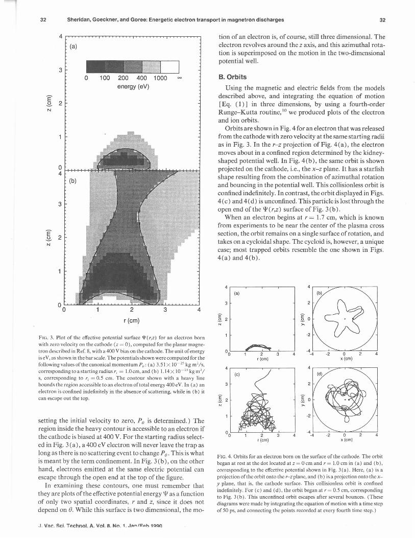
FIG. 3. Plot of the effective potential surface 'i'(r,z) for an electron born with zero velocity on the cathode (z = 0), computed for the planar magne­tron described in Ref. 8, with a 400 V bias on the cathode. The unit of energy is eV, as shown in the bar scale. The potentials shown were computed for the following values of the canonical momentum P0 : (a) 3.51 X 10- 25 kg m2/s, corresponding to a starting radius r, = 1.0 cm, and (b) 1.14 X 10- 25 kg m2 I s, corresponding to r, = 0.5 cm. The contour shown with a heavy line bounds the region accessible to an electron of total energy 400 eV. In (a) an electron is confined indefinitely in the absence of scattering, while in (b) it can escape out the top.

setting the initial velocity to zero, Pe is determined.) The region inside the heavy contour is accessible to an electron if the cathode is biased at 400 V. For the starting radius select­ed in Fig. 3(a), a 400 eV electron will never leave the trap as long as there is no scattering event to change Pe. This is what is meant by the term confinement. In Fig. 3 ( b), on the other hand, electrons emitted at the same electric potential can escape through the open end at the top of the figure.

In examining these contours, one must remember that they are plots of the effective potential energy 'JI as a function of only two spatial coordinates, r and z, since it does not depend on e. While this surface is two dimensional, the mo-

.I. Var:. Sci. Technol. A. Vol. 8. No. 1. J""'"'"h 1!l!l0

tion of an electron is, of course, still three dimensional. The electron revolves around the z axis, and this azimuthal rota­tion is superimposed on the motion in the two-dimensional potential well.

B. Orbits

Using the magnetic and electric fields from the models described above, and integrating the equation of motion [Eq. ( 1)] in three dimensions, by using a fourth-order Runge-Kutta routine, w we produced plots of the electron and ion orbits.

Orbits are shown in Fig. 4 for an electron that was released from the cathode with zero velocity at the same starting radii as in Fig. 3. In the r-z projection of Fig. 4(a), the electron moves about in a confined region determined by the kidney­shaped potential well. In Fig. 4(b ), the same orbit is shown projected on the cathode, i.e., the x-z plane. It has a starfish shape resulting from the combination of azimuthal rotation and bouncing in the potential well. This collisionless orbit is confined indefinitely. In contrast, the orbit displayed in Figs. 4 ( c) and 4 ( d) is unconfined. This particle is lost through the open end of the 'JI ( r,z) surface of Fig. 3 ( b).

When an electron begins at r = 1.7 cm, which is known from experiments to be near the center of the plasma cross section, the orbit remains on a single surface of rotation, and takes on a cycloidal shape. The cycloid is, however, a unique case; most trapped orbits resemble the one shown in Figs. 4(a) and 4(b) .

4 4

(a} (b}

3

K 2 N

2

~ Ko >-

-2

00 3 4 -4

-4 -2 0 2 4 x(cm}

4 4

(c}

3 2

K 2 Ko N >-

-2

3 4 -2

FIG. 4. Orbits for an electron born on the surface of the cathode. The orbit began at rest at the dot located at z = 0 cm and r = 1.0 cm in (a) and (b), corresponding to the effective potential shown in Fig. 3(a). Here, (a) is a projection of the orbit onto the r-z plane, and (b) is a projection onto the x­

Y plane, that is, the cathode surface. This collisionless orbit is confined indefinitely. For (c) and (d), the orbit began at r = 0.5 cm, corresponding to Fig. 3(b). This unconfined orbit escapes after several bounces. (These diagrams were made by integrating the equation of motion with a time step of 50 ps, and connecting the points recorded at every fourth time step.)

33 Sheridan, Goeckner, and Goree: Energetic electron transport in magnetron discharges 33

In all cases, the paths of energetic electrons do not have the helical shape characteristic ofLarmor orbits. This is a conse­quence of the gyroradius being comparable to the scale length of the magnetic field. The orbits revolve around the z axis in the EX B direction.

Ion trajectories computed for the planar magnetron de­vice are shown in Fig. 5. They differ markedly from the or­bits of electrons as a consequence of their higher mass. In effect, the ions are not mag:r:ietized. They fall directly to the cathode with very little radial displacement. This observa­tion is used in the physical model of energetic electron trans­port that we develop next.

Ill. TRANSPORT MODEL

In Sec. II we showed that there are electron orbits that are confined indefinitely in a trap in the absence of some scatter­ing mechanism. This serves as motivation for the need to model transport. In this section, we will describe a physical model in which the energetic electrons are scattered by colli­sions with neutrals.

A. Assumptions

Our model portrays single electrons as if they respond to prescribed, time-independent E and B fields and suffer colli­sions at random intervals. Collective plasma effects, which would alter the fields and change an electron's energy, are neglected. The ions are treated as if they are unmagnetized. They fall directly from their point of origin toward the cath­ode; assuming a one-dimensional electric field , they fall without any radial deflection. When they strike the cathode, the ions create secondary electrons that initially have a ki­netic energy of typically 1-4 e V, 11 which we approximate to be zero.

Initially, two types of electron collisions, with neutrals and with ions, must be evaluated. Consider a typical magne­tron discharge having an ion density of2X 10 10 cm - 3 and room temperature argon at a pressure of 1 Pa. For a 400 eV electron, the perpendicular momentum deflection collision frequency is 14 MHz for scattering by neutrals, but only 250 Hz for scattering by ions. Accordingly, we neglect Coulomb collisions in our magnetron model.

4 4 (a) (b)

3 2

:[ 2 :[ 0 N >-

I I I I I I I I I -2

00 2 3 4 -4

-4 -2 0 2 4

r(cm) x (cm)

FIG. 5. Orbits of ions born at z = I cm. The paths followed by Ar+ are shown for several initial radii. The ions are released at z = I cm with zero initial velocity, and then the presheath electric field accelerates them to the surface of the cathode. As they fall, they are deflected slightly in the azi­muthal direction, but only a negligible amount in the radial direction. The electric potential is assumed here to vary with z but not r.

J. Vac. Sci. Technol. A, Vol. 8, No. 1, Jan/Feb 1990

B. Neutral collisions

The history of a fast electron can be summarized as fol­lows. After it is created on the cathode or in the sheath, it falls down the potential hill of the sheath, gaining energy. It slowly loses this energy due to collisions with neutrals. Meanwhile, the orbit swirls about in the potential well, and it may or may not be trapped. Every time a collision takes place, an electron that is trapped may be scattered into an unconfined orbit and become lost from the system. Thus, some fast electrons will be confined long enough to perform a large number of ionizations, while others will be present only long enough to perform a few or even none at all. As a result of all these ionizations, the bulk electron population is formed.

In our treatment, three types of collisions with neutrals are taken into account: elastic scattering, ionization, and ex­citation. All these collisions result in scattering the direction of the electron's velocity and reducing its energy. However, several collision processes are neglected. We do not allow for the possibility of a single collision resulting in either a double ionization (which accounts for 6% of the toal inelastic cross section atE = 100 eV), nor do we allow the production of an excited state of an ion (which accounts for less than 1 % of the total). 12 Additionally, Penning ionization and two-step ionization are not accounted for.

The energy lost in a collision depends on its type. Ionizing events result in the greatest energy Joss, which is the ioniza­tion potential ( 15.8 eV for ground state argon) plus the ki­netic energy of the newly released electron. The energy Jost in an excitation collision ( 11.6-15.8 eV for argon) depends on the energy level to which the neutral is excited. Of the three types of collisions, an elastic scattering consumes the least energy. The fractional loss is on the order of the mass ratio, !1K /K = (4me/M) sin2 (a/2), where m e and Kare the mass and kinetic energy of the electron, Mis the mass of the neutral, and a is the angle by which the velocity is de­flected.

All three types of collisions are characterized by a differ­ential scattering cross section da/dfl that predicts the prob­ability per unit solid angle of scattering into an angle a for a given energy K. For ionization collisions in particular, a full differential cross section would also be specified as a func­tion of the energy of the newly created electron. 13

The angular dependence of the differential cross secion dcr/ dfl varies with energy. For most gases, the cross sections are nearly isotropic for low electron energies, while for K> 60 eV they are generally peaked for small values of a, i.e., for foward scattering.

This predominance of forward scattering means that Pe and consequently 'I' are not changed greatly in most colli­sions. Hence, an electron may suffer many collisions before it is scattered out of a confining well. If the confinement is effective, energetic electrons may use up almost all of their energy before they are lost, therby maximizing the ion pro­duction.

IV. NUMERICAL IMPLEMENTATION

In the physical model described above, electrons move in prescribed electric and magnetic fields, subject to collisions

I

34 Sheridan, Goeckner, and Goree: Energetic electron transport in magnetron discharges 34

at random intervals. This type of model is well suited for application in a Monte Carlo computer code. Using such a code involves following the orbits of a large number of elec­trons one at a time; keeping track of their location, velocity, and kinetic energy; and allowing them to scatter in colli­sions. To do this, we must provide expressions for the elec­tric and magnetic fields, push the electrons with an integra­tor based on the equation of motion, and provide accurate differential scattering cross sections. Additionally, the use of Monte Carlo codes requires that initial conditions for each particle be chosen in an unbiased fashion to obtain meaning­ful results.

We have implemented our physical model with a fully three-dimensional Monte Carlo program. In this section, we describe its operation and list the approximations that it en­tails.

A. Integrating the orbits

The equation of motion to be integrated is Eq. ( 1). It is integrated in single steps according to a fixed time step at by using the same fourth-order Runge-Kutta method as in Sec. II. To follow the orbit accurately, the value of Mis chosen to be small compared to both the gyroperiod and the inverse collision frequency and to provide energy conservation.

The electric and magnetic fields used here are the same as those described in Sec. II. The magnetic field is recorded in a two-dimensional grid in the r-z plane, while the electric field is gridded in one coordinate z. Interpolation is used to evalu­ate the fields between grid points.

B. Collisions

At each time step during an electron orbit, we determine whether a collision has taken place. This is done by generat­ing a random number that is compared to the probability per unit time of a collision. For argon, we use the total cross sections reported in Refs. 14 and 15, and interpolate between tabulated values.

When it has been determined that a collision takes place, another random number is generated to determine whether it was an elastic, excitation, or ionization event. This is evalu­ated according to the relative cross sections of these pro­cesses.

According to the type of collision, the energy of the ener­getic electron is reduced. In our current code we approxi­mate that the energy lost in an excitation or ionizing collision is always a fixed amount, 11.6 eV for excitation and 15.8 eV for ionization of argon. By using a fixed energy loss for ioni­zation, we ignore the kinetic energy of the secondary elec­tron released in an ionization event. That energy is almost always much smaller than the energy of the ionizing elec­tron. 13 Accordingly, we use a reduced scattering cross sec­tion for ionization that does not depend on the energy of the secondary electron.

In addition to decrementing the energy of the energetic electron when it undergoes a collision, we randomly scatter its velocity into a new direction, which is chosen in a manner consistent with the differential scattering cross section. For the energy range K < 3 eV, we assume that the differential

J. Vac. Sci. Technol. A, Vol. 8, No. 1, Jan/Feb 1990

cross sections are isotropic. For 3 eV <K < 3 keV, we use the normalized values of do/ dfl for elastic scattering that are tabulated in Ref. 16. We make the approximation that these are valid for all three types of collisions. The suitability of this simplification can be confirmed by an inspection of the shapes of do I dfl as a function of energy for the three types of collisions, 13 which reveals that they are nearly the same.

C. Ensembles of orbits

An orbit must be terminated according to some criterion, such as: ( 1) it leaves the simulation region, ( 2) a fixed maxi­mum time has elapsed, or ( 3) the energy is depleted below the level of the ionization potential. When this happens, a new energetic electron orbit is begun from a new initial posi­tion. This is repeated for an ensemble of electrons. After the last electron is finished, the user can produce useful results such as a spatial profile of ionization events.

The statistical quality of those results will be determined by both random and systematic errors. Random errors di­minish according to the square root of the number of elec­trons in the ensemble. The larger the ensemble size, the smaller the random errors will be. Of course the computer time required increases linearly with the number of elec­trons, so the user cannot choose the ensemble size to be arbi­trarily large but rather chooses it to give the size of error bars desired.

On the other hand, systematic errors are generally not improved upon by increasing the ensemble size. They must be eliminated by thoughtful planning of the code. One poten­tial source of systematic errors that requires special attention in all Monte Carlo codes is the choice of the initial conditions for each electron.

D. Initial conditions

Physically, the position at which each electron starts is different. Accordingly, in the numerical implementation, a different random starting position must be chosen for each electron. This must be done in a fashion that represents the physical processes involved. The code could be used with initial conditions chosen to simulate electrons born in the plasma and sheath regions, but in the present paper, we will treat only the electrons originating on the cathode due to ion bombardment.

The starting radius r; for each electron is specified in the following convergent manner. The first electron is released from a random point. Subsequent electrons can originate from any point on the cathode, with some points more likely than others. To account for this, we use a radial probability profile P( r; ) to describe the probability per unit radius of an electron being born at r;. Physically, each electron is respon­sible for ionizations that would result in ions falling directly down to the cathode, resulting in the emission of new elec­trons at the sites of ion impact. Accordingly, in the code, P( r;) is updated according to the history of all previous ion­izations before starting each new electron. This is done by counting the ionizations that took place in radial bins.

The probability profile converges to a recognizable steady state after about 30 fast electrons have been tracked. This

35 Sheridan, Goeckner, and Goree: Energetic electron transport in magnetron discharges 35

means that for many applications the code must be run for an ensemble of more than 30 electrons.

V.RESULTS As a test of the numerical implementation of our physical

model, we ran an ensemble of 600 electrons originating at the cathode. The discharge was assumed to have the parameters of the experiment reported in Ref. 7: cathode bias of 400 V, argon gas pressure of 1 Pa, Te = 4 eV, and density appropri­ate to produce a Debye length ofO. l mm. Under these condi­tions, the total collision mean free path is 1. 7 cm for a 20 e V electron, and 9.4 cm for a 400 eV electron.

The time step 6.t was selected to be 50 ps. This value was chosen to be small enough to provide 20 integration steps per gyroperiod in a 300 G magnetic field. It also provided at least 130 steps per collision, on average.

Orbits were followed until the electrons either escaped from the boundaries of our 4 X 4 cm working space on the r-z plane or until a limit of 2.5 µshad elapsed, whichever came first. The time limit was chosen to be long enough that fewer than 0.5% of the remaining electrons had enough energy to result in an ionization. For this run, we did not stop orbits if the electron energy fell below the 15.8 eV ionization poten­tial of argon.

A. Collision statistics

We recorded the location and type of each collision. De­fining the average number of ionizations per fast electron as (N, ), our run yielded (N,) = 14.26 ± 0.44, where the un­certainty given is for a 90% confidence level. For compari­son, consider that a 400 eV electron can produce at most Nmax = 25 ionizations, given the ionization potential of 15.8 e V for argon.

Note that ifthe discharge is to be maintained solely by ion bombardment of the cathode, then it is necessary that (N,) >r- 1

, where y is the secondary electron emission coef­ficient. Since y- 1

::::::: 10 for many metals, our result that (N,)::::::: 14 confirms that cathode emission alone could sus­tain a magnetron plasma.

For the same ensemble of 600 fast electrons, there were an average of 3.65 ± 0.16 excitation collisions per electron. This number is less than (N,) simply because the cross sec­tion for excitation is smaller than that for ionization.

The most frequent type of collision is elastic, because of its large cross section, especially for lower energies. Our ensem­ble experienced 48.67 elastic collisions per electron. Most of these occurred after the energy of a trapped electron had been depleted below the 11.6 eV excitation potential, where there is no possibility of inelastic collisions.

The distribution of the number of ionizing collisions per electron is shown in a histogram, Fig. 6. The most probable number of ionizations per fast electron was 20, which is at the center of a peak between 18 and 24 ionizations per elec­tron. (The width of this peak is accounted for by excitation collisions.) Recalling the Nmax is 25, we see that this peak indicates that many fast electrons remained trapped until most of their energy is lost. The other electrons performed a smaller number of ionizations and then escaped.

The confinement provided in an actual magnetron plasma J

J. Vac. Sci. Technol. A, Vol. 8, No. 1, Jan/Feb 1990

60 CJ)

c e t5 QJ

Qi 0 40 iii .0 E :::J c

20

0 5 10 15 20 25

FIG. 6. Distribution of number of ionizing collisions for 600 electrons in argon at a pressure of I Pa. This histogram has a peak centered at 20 ioniza­tions, which corresponds to electrons that lose all their energy in collisions without escaping from the trap. Elastic, excitation, and ionizing collisions are taken into account. The maximum possible number of ionizations is Nma• = 25, which is the ratio of the 400 V cathode potential to the 15.8 eV ionization potential. The width of the peak is due to energy lost in excitation collisions.

works well, producing almost as many ionizations as possi­ble. This is of course the advantage of the magnetron as a sputtering device.

The principal reason for the good confinement is the effec­tive potential well. Furthermore, as we discussed at the end of Sec. Ill, most differential cross sections are peaked for forward scattering, which means that to scatter P8 enough to detrap the electron, many collisions may be required. To test this prediction, we performed a run for comparison where do/df! was isotropic and found that (N,) was 2.52 ± 0.15, which is small compared to the value of 14.26 reported above. This indicates that in contrast to forward scattering, large angle scattering leads to a loss of confine­ment after fewer ionizations have occurred. Much of the magnetron's high ionization efficiency can thus be attribut­ed to the predominance of forward scattering.

B. Density of ionizing collisions

The density of ionization collisions p1 (r,z) is shown in Fig. 7. Recalling that the z axis is the axis of symmetry for the planar magnetron, an inspection of this illustration reveals that the ionization events are concentrated in a ring located above the cathode surface. Some of the ionization events from Fig. 7 were used to prepare Fig. 1, where the ring is shown in a three-dimensional view. The latter diagram bears a very close resemblance to the visual appearance of a planar magnetron discharge.

According to the physical model of electron transport, the ionization distribution is determined by electron orbits, which are determined by the shape of the effective potential

36 Sheridan, Goeckner, and Goree: Energetic electron transport in magnetron discharges 36

3

E 2 ~

N ' ... ··:. ·.· .. _.· .. .... ·: . .. . . , ..

relative number of ionization collisions

1

0.8

0.6

0.4

0.2

0 '--~~~--L~-'"--'="-~=---=-'~~~~~~~~ 0 2

r(cm) 3 4

FIG. 7. Density of ionizing collisions, p; ( r,z), plotted as a function of rand z. The locations of the ionization events were assigned to pixels 0.5 X 0.5 mm in size to produce the gray-scale diagram. In pixels having less ionization than the bottom of the gray scale, the event locations are shown with dots. The region of strong ionization forms a ring separated from the cathode surface by a dark space. Note the similarity to the effective potential 'i'(r,z) shown in Fig. 3(b). The event locations indicated here were used in prepar­ing the three-dimensional view in Fig. I.

well. It is therefore instructive to comparep; (r,z) in Fig. 7 to an effective potential well shape, such as Fig. 3. The shapes are nearly the same, even though a large number of potential wells were sampled by the electrons. This finding is consis­tent with the descriptive model of electron motion presented in Sec. II.

C. Radial profile of ionizations

A useful quantity that can be obtained fromp; (r,z) is the radial ionization profile,

n, (r) = -1-J p; (r,z)dz

21Tr (4)

which represents the number of ionizations per unit area above the cathode. Recall that in our model, the ions fall directly down to the cathode from the ionization site without radial deflection. Therefore, n, (r) can be directly compared to experimental measurements of the radial profile of the ion flux striking the cathode.

This ion flux is easy to measure. One indication is the depth of the etch track in the cathode material. After a num­ber of hours of operating our planar magnetron in argon, we measured the etch track profile in the copper cathode. 7 It had a maximum depth of 2 mm. In Fig. 8 a plot of this experimentally obtained profile is overlaid on a plot of the radial ionization distribution computed from our Monte Carlo results. The agreement between the model and the experimental data is good.

This comparison is successful despite the fact that the etch track was formed by operating the magnetron at a number of

J. Vac. Sci. Technol. A, Vol. 8, No. 1, Jan/Feb 1990

~ -~ iii E io.5 c~

2

1.5 ~

0.5

::r

~ "A 0. (1) -g ::r

3 2.

w_-=-~~-'-~~~-'--~~-"--=~~~--'O

2 r(cm)

3 4

FIG. 8. Radial profile of ionizing collisions, n, (r), from the simulation, compared to etch track depth from experimental measurements. The verti­cal scales for the two curves were adjusted to make the heights of their peaks match. The agreement is good.

different pressures and cathode biases. (Better experimental data could be obtained in the fashion of Wendt et al. by imbedding current probes in the magnetron cathode sur­face. 5)

Our finding that the shape of the etch track can be predict­ed accurately lends confidence to the model.

D. Axial profile of ionizing collisions

Inelastic collisions produce the optical emission from a magnetron discharge. For most atomic gases, the visible light that an observer can see originates from transitions between the excited states. Consequently, the optical emis­sion from a magnetron can be modeled by recording the lo­cations of the inelastic collisions that result in exciting the neutral to a highly excited state.

As a proxy for excitations to those highly excited states, here we will use the ionization events. This is a suitable ap­proximation because the total ionization and excitation cross sections have nearly the same dependence on electron energy.

The axial distribution of ionizing collisions n, (z) was computed by integrating the ionization density radially and is shown in Fig. 9. Note the appearance in this illustration of a cathode dark space between 0 < z < 2 mm. There is also a peak inn, (z) at z = 3 mm.

This figure can be compared to an experimental measure­ment of axial distribution of optical emission, which will also display a dark space as well as a peak in the emission a few millimeters from the cathode. Such a measurement was re­ported by Gu and Lieberman. 17 They used an optical appa­ratus that had an axial spatial resolution of 0.28 mm to detect the total visible emission along a radial chord. Their experiment is suited for a test of our numerical results shown in Fig. 9, although the comparison can only be qualitative because we used a different magnetic configuration. We do find qualitative agreement between our simulation and their experiment.

37 Sheridan, Goeckner, and Goree: Energetic electron transport in magnetron discharges 37

3

E ~ 2 N

200 400 600 800

FIG. 9. Axial profile of ionizing collisions from the model, n, (z). The cath­ode is located at z = 0. This can be compared to experimental measure­ments of the axial optical emission profile, such as the one reported in Ref. 17. Note the appearance of a cathode dark space for 0 < z < 2 mm.

VI. CONCLUSIONS

We have presented a model of energetic electron transport in magnetron plasmas. This single particle description is ap­plicable to all magnetron geometries. We have reduced the problem by making a number of approximations. Most nota­bly, we allow scattering of electrons by only three types of collisions (ionization, excitation, and elastic scattering), and we track single electron orbits in prescribed magnetic and electric fields .

We have applied the model by developing a Monte Carlo orbit code. For the present purposes, we used it to gain an understanding of the physical processes involved in magne­tron discharges, although it may also be practical for design­ing optimum magnetron configurations.

As a test of the Monte Carlo method, we simulated the electrons emitted from the cathode of a planar magnetron. A two-dimensional B field and a one-dimensional E field were assumed. We found that cathode emission results in an aver-

J. Vac. Sci. Technol. A, Vol. 8, No. 1, Jan/Feb 1990

age of 14.26 ionizations per electron for a 400 V discharge in argon at a pressure of 1 Pa. This high efficiency of ionization is attributable to the electron confinement brought about by the magnetron's effective potential well and by the predomi­nance of forward scattering. The spatial distribution of ioni­zation predicted in the simulation was compared to experi­mental measurements of the radial ion current profile and the axial optical emission profile. These tests show good agreement between theory and experiment, indicating that the model can accurately characterize the locations in the discharge where ionization takes place.

ACKNOWLEDGMENTS

The authors thank Mark Kushner and Amy Wendt for helpful discussions. This work was funded by a grant from the Iowa Department of Economic Development and an IBM Faculty Development Award.

'John A. Thornton and Alan S. Penfold, in Thin Film Processes, edited by J. L. Vossen and W. Kern (Academic, New York, 1978) , p. 75.

2Robert K. Waits, in Ref. I, p. 131. 3David B. Fraser, in Ref. I, p. 115. 4 Francis F. Chen, Introduction to Plasma Physics and Controlled Fusion, 2nd ed. (Plenum, New York, 1984) , p. 190.

5 A. E. Wendt, M. A. Lieberman, and H. Meuth, J. Vac. Sci. Technol. A 6, 1827 ( 1988), and A. E. Wendt, Ph.D. thesis, University of California at Berkeley, 1988.

6S. M. Rossnagel and H. R. Kaufman, J. Vac. Sci. Technol. A 6, 223 (1988).

7T. E. Sheridan and J. Goree, J. Vac. Sci. Technol. A 7, 1014 ( 1989). "George Schmidt, Physics of High Temperature Plasmas, 2nd ed. (Aca­demic, New York, 1979) , Secs. 2-6.

"T. E. Sheridan and J. Goree, U. of Iowa Report No. 89-13, IEEE Trans. Plasma Sci. (in press).

'0 C. E. Roberts, Ordinary Differential Equations: A Computational Ap­proach (Prentice-Hall, Englewood Cliffs, NJ, 1979).

"David B. Medved and Y. E. Strausser, Adv. Electronics Electron Phys. 21, IOI ( 1965).

12R. J. Carman, J. Phys. D 22, 55 ( 1989). "E. W. McDaniel, Collision Phenomena in Ionized Gases (Wiley, New

York, 1964). '4Makato Hayashi, Nagoya Institute of Technology Report No. IPPJ-AM-19, Research Information Center, !PP/Nagoya University, Nagoya, Ja­pan, 1981 , errata 1982.

15F. J. deHeer, R. H.J. Jansen, and W. van der Kaay, J. Phys. B 12, 979 ( 1979).

'6S. N. Nahar and J.M. Wadehra, Phys. Rev. A 35, 2051 ( 1987).

17Lan Gu and M.A. Lieberman, J. Vac. Sci. Technol. A 6, 2960 (1988).