model predictive control of water quality in drinking ...etheses.bham.ac.uk/7207/1/xie17phd.pdf ·...
TRANSCRIPT
MODEL PREDICTIVE CONTROL
OF WATER QUALITY IN
DRINKING WATER
DISTRIBUTION SYSTEMS
CONSIDERING DISINFECTION
BY-PRODUCTS
by
MINGYU XIE
A thesis submitted to
The University of Birmingham
for the degree of
DOCTOR OF PHILOSOPHY
Department of Electronic,
Electrical and System Engineering
University of Birmingham
September 2016
University of Birmingham Research Archive
e-theses repository This unpublished thesis/dissertation is copyright of the author and/or third parties. The intellectual property rights of the author or third parties in respect of this work are as defined by The Copyright Designs and Patents Act 1988 or as modified by any successor legislation. Any use made of information contained in this thesis/dissertation must be in accordance with that legislation and must be properly acknowledged. Further distribution or reproduction in any format is prohibited without the permission of the copyright holder.

To my wife and parents
ACKNOWLEDGEMENT
First and foremost, I would like to express my sincere gratitude to my first supervisor
Prof. Xiao-Ping Zhang, for his patience, guidance and encouragement during my PhD
study. His invaluable support greatly helped me to overcome the difficulty in my
research period and to continue with my research. It is a great honour for me to be a
student of Prof. Zhang.
I would like to thank another supervisor Prof. Mietek A. Brdys. He gave me the
opportunity to conduct my PhD study and he guided me at the beginning of my PhD
study. His patience, guidance and professional academic support greatly facilitated
my PhD research.
In addition, I would like to thank my co-supervisor Dr. Dilan Jayaweera, for his
professional suggestions and patient guidance while conducting my PhD research.
I also wish to express my appreciation to my colleagues Dr. Suyang Zhou, Dr. Zhi Wu,
Dr. Puyu Wang, Dr. Jing Li, Dr. Ying Xue, Ms. Can Li, Mr. Hao Fu, Mr Mao Li and all
my other colleagues in the Power and Control Group for their kind advice and
assistance. It was an enjoyable experience to work alongside them.
Finally, I must express my greatest appreciation to my parents, Mr. Chuanda Xie and
Mrs. Linwei Song, for their endless love and support throughout my life so far. I must

thank my wife Ms. Qing Wang, for her support and love given throughout my PhD
study.
ABSTRACT
The shortage in water resources have been observed all over the world. However, the
safety of drinking water has been given much attention by scientists because the
disinfection will react with organic matters in drinking water to generate disinfectant
by-products (DBPs) which are considered as the cancerigenic matters. The
health-dangerous DBPs have brought potential hazards to people’s daily lives.
Therefore investigating the nonlinear water quality model in drinking water
distribution systems (DWDS) considering DBPs and controlling both disinfection and
DBPs in an appropriate way are the basis of the research of this thesis.
Although much research has been carried out on the water quality control problem in
DWDS, the water quality model considered is linear with only chlorine dynamics, the
existence of DBPs caused by reactions between chlorine and organic matters has not
been considered in the linear model. In addition, only the disinfectant (chlorine) is
considered as the objective of water quality control. Compared to the linear water
quality model, the nonlinear water quality model considers the interaction between
chlorine and DBPs dynamics which follow the reaction fact in the DWDS.
The thesis proposes a nonlinear model predictive controller which utilises the newly
derived nonlinear water quality model as a control alternative for controlling water
quality. Dealing with the optimisation problem under input and output constraints
requires advanced algorithm to handle the difficulty brought by nonlinear dynamic
model. In this thesis, the model predictive control (MPC) algorithm is the main driver
for solving the nonlinear, constrained and multivariable control problem. EPANET
and EPANET-MSN are simulators utilised for modelling in the developed nonlinear
MPC controller.
However, uncertainty is not considered in these simulators because these simulators
only measure the simulation data under given control inputs. Methods of modelling
the nonlinear water quality model with considering uncertainty are required for
controlling water quality with DBPs properly. Hence, the method called
point-parametric model (PPM) is utilised to obtain the bounded nonlinear water
quality model jointly considering the uncertainty and structure error. This thesis
proposes the bounded PPM in a form of multi-input multi-output (MIMO) to robustly
bound parameters of chlorine and DBPs jointly and to robustly predict water quality
control outputs for quality control purpose.
The methodologies and algorithms developed in this thesis are verified by applying
extended case studies to the example DWDS. The simulation results are critically
analysed, which demonstrate the viability of the developed controller and algorithms.
i
Table of Contents
ACKNOWLEDGEMENT I
ABSTRACT I
Table of Contents i
List of Figures ix
List of Tables xii
List of Abbreviations xiii
CHAPTER 1 INTRODUCTION 1
1.1 Background and Motivation 1
1.1.1 Water Supply/Distribution Systems 1
1.1.2 Chlorination of Drinking Water in the Chemical Process 5
1.1.3 Disinfection by Products 7
1.1.4 Advanced Water Quality Control Algorithm-Model Predictive Control 10
1.1.5 Motivations 12
ii
1.2 Aims and Objectives 14
1.3 Contributions 17
1.4 Thesis Outlines 18
CHAPTER 2 LITERATURE REVIEW 21
2.1 Overview of Operational Control on Drinking Water Distribution
Systems 21
2.1.1 Review on Quantity Control in Drinking Water Distribution Systems 24
2.1.2 Review on Chlorine Residual Control in Drinking Water Distribution
Systems 26
2.1.3 Review on Disinfectant by-Products: History, Formation, Regulation and
Control 30
2.1.4 Integrated Control of Both Quality and Quantity in DWDS 35
2.1.5 Placement of Booster Stations and Hard Sensors in Drinking Water
Distribution Systems 37
2.1.6 Monitoring by Soft Sensors on Water Quality in DWDS 41
2.2 Model Predictive Control Overview 42
iii
2.2.1 Linear Model Predictive Control 43
2.2.2 Nonlinear Model Predictive Control 45
2.2.3 Robust Model Predictive Control 49
2.2.4 Optimisation Overview in Model Predictive Control 51
2.3 Review on Genetic Algorithm 52
2.4 Summary 54
CHAPTER 3 OPERATIONAL CONTROL AND MODELLING IN
DRINKING WATER DISTRIBUTION SYSTEMS 56
3.1 Fundamentals of operational control in Drinking Water Distribution
Systems 57
3.1.1 Objectives of Operational Control 58
3.1.2 Handling Uncertainties 59
3.1.3 Basic Control Mechanisms 60
3.2 Characteristics of Hydraulic Components and Physical Laws in
Drinking Water Distribution Systems 60
3.2.1 Pipes 62
iv
3.2.2 Valves 64
3.2.3 Pumps 65
3.2.3.1 Fixed Speed Pumps 65
3.2.3.2 Variable Speed Pumps 67
3.2.3.3 Variable Throttle Pumps 68
3.2.3.4 Pump Station 69
3.2.4 Reservoirs 70
3.2.5 Physical Laws 72
3.2.5.1 Flow Continuity Law 72
3.2.5.2 Energy Conservation Law 74
3.3 Path Analysis Algorithm 74
3.3.1 Detention Time Calculation in a Pipe 76
3.3.2 Detention Time Calculation in a Path 78
3.3.3 Discretization of Time Delay 79
3.4 Summary 80
v
CHAPTER 4 APPLICATION OF NONLINEAR MODEL PREDICTIVE
CONTROL ON WATER QUALITY IN DWDS WITH DBPS INVOLVED 82
4.1 Introduction to the Hierarchical Two-Level Structure in DWDS 83
4.2 Quality Model Dynamics with Considering DBPs 89
4.2.1 Dynamics of the quality kinetics 89
4.2.2 Quality dynamic model 90
4.3 Optimising Model Predictive Controller for Water Quality with
Augmented DBPs Objective 93
4.3.1 Model Predictive Control Methodology 94
4.3.2 Formulation of MBOP 96
4.3.3 State Feedback 96
4.3.4 Solver of MBOP 97
4.3.5 Model Simulator: EPANET AND EPANET-MSX 98
4.4 Application to Case Study DWDS and Simulation Results 99
4.4.1 Case Study Network and Design of Nonlinear MPC controller 99
vi
4.4.2 Software Implementation 103
4.4.3 Simulation Results 103
4.5 Summary 111
CHAPTER 5 ROBUST PARAMETER ESTIMATION AND OUTPUT
PREDICTION ON NONLINEAR WATER QUALITY MODEL IN DWDS
WITH CONSIDERING DBPS 112
5.1 Introduction 113
5.2 MIMO Structure of PPM in IO Model 115
5.2.1 IO model of water quality in DWDS with Considering DBPs 115
5.2.2 MIMO Point-Parametric Model 118
5.2.2.1 Mathematical Model of MIMO Point-Parametric Model 118
5.2.2.2 Structure of information exchange 121
5.2.2.3 Robust Parameter Estimation 122
5.2.2.4 Experiment Design 124
5.2.2.5 Validation of the MIMO PPM 126
vii
5.2.3 Robust Output Prediction by Implementing Piece-Wise Constant
Continuity in Model Parameters 128
5.3 Simulation Results and Discussions 131
5.3.1 Example network with one switching type tank 131
5.3.2 Illustration of Path Analysis Algorithm 133
5.3.3 Simulation Results and Discussions 135
5.4 Summary 139
CHAPTER 6 CONCLUSION AND FUTURE RESEARCH WORK 141
6.1 Conclusions 141
6.2 Future Research Work 143
LIST OF PUBLICATIONS 145
APPENDIX A EPANET INPUT FILE FOR EXAMPLE NETWORK 146
APPENDIX B EPANET-MSX INPUT FILE FOR EXAMPLE NETWORK 152
APPENDIX C AN EXAMPLE C-MEX FILE FOR CALLING EPANET IN
MATLAB 155

viii
REFERENCE 158
ix
List of Figures
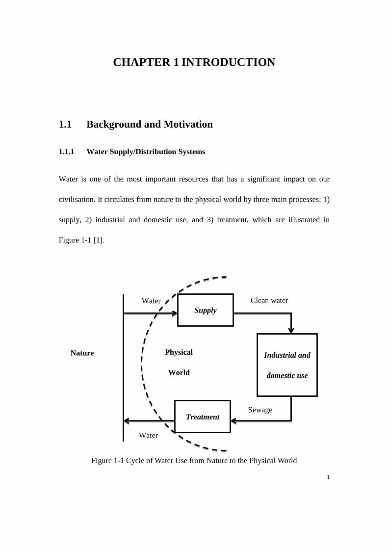
Figure 1-1 Cycle of Water Use from Nature to the Physical World .............................. 1
Figure 1-2 Structure of water supply/distribution systems ............................................ 2
Figure 1-3 Presentation of a treatment works ................................................................ 4
Figure 3-1 Overview of an Example DWDS ............................................................... 57
Figure 3-2 Model of a Single Pipe ............................................................................... 62
Figure 3-3 Model of Variable Control Valve Equipped in A Pipe .............................. 65
Figure 3-4 Generalized Pump Station Configuration [1] ............................................. 70
Figure 3-5 Model of a Reservoir .................................................................................. 71
Figure 3-6 Connection Node ........................................................................................ 73
Figure 3-7 Water flow velocity in a pipe ..................................................................... 76
Figure 3-8 Backward Tracking in A Pipe .................................................................... 77
Figure 3-9 Illustration of Transportation Paths in a DWDS ........................................ 78
Figure 3-10 Continuous Time Delay during Modelling Horizon ................................ 79
x
Figure 4-1 Hierarchical Two-Level Structure for Optimising Control of Integrated
Quantity and Quality [13] .................................................................................... 86
Figure 4-2 The Basic MPC Control Loop [13] ............................................................ 94
Figure 4-3 Case Study DWDS Network .................................................................... 100
Figure 4-4 Working Procedure of Developed Nonlinear MPC Controller ................ 102
Figure 4-5 Chlorine Concentration at Monitored Node under 11 hours of Draining
Cycle .................................................................................................................. 105
Figure 4-6 DBP Concentration at Monitored Node under 11 hours of Draining Cycle
............................................................................................................................ 105
Figure 4-7 Chlorine Concentration at Monitored Node under 6.8 hours of Draining106
Figure 4-8 DBP Concentration at Monitored Node under 6.8 hours of Draining Cycle
............................................................................................................................ 107
Figure 4-9 Chlorine Concentration at Monitored Node under 9.5 hours of Draining107
Figure 4-10 DBP Concentration at Monitored Node under 9.5 hours of Draining Cycle
............................................................................................................................ 108
Figure 4-11 Chlorine Concentration at Monitored Node Obtained by MPC Controller
without Considering DBP under 11 hours of Draining Cycle ........................... 110
xi
Figure 4-12 DBP Concentration at Monitored Node Obtained by MPC Controller
without Considering DBP under 11 hours of Draining Cycle ........................... 110
Figure 5-1 PPM Information Structure ...................................................................... 122
Figure 5-2 The Case Study Network with a Switching Tank .................................... 132
Figure 5-3 Path Analysis to the Case Study Network ................................................ 134
Figure 5-4 Detention Time in Three Active Paths during the Whole Modelling Horizon
............................................................................................................................ 134
Figure 5-5 Parameter Bounds Corresponding to Delay Number 13 in Chlorine ....... 135
Figure 5-6 Parameter Bounds Corresponding to Delay Number 13 in DBPs ........... 135
Figure 5-7 Robust Output Prediction on Chlorine under Unit Step Input ................. 136
Figure 5-8 Robust Output Prediction on DBPs under Unit Step Input ...................... 136
Figure 5-9 Robust Output Prediction on Chlorine under Random Input ................... 137
Figure 5-10 Robust Output Prediction on DBPs under Random Input ..................... 138
xii
List of Tables
Table 2-1 Major groups of DBPs ................................................................................. 33
Table 2-2 Strategies for Controlling halogenated DBPs formation ............................. 34
Table 4-1 The Total Amount and Average Amount of DBP Concentration at Monitored
Node under Different Scenarios......................................................................... 108
Table 5-1 Uncertainty Radius within Different Weight Coefficient Sets .................. 139
xiii
List of Abbreviations
ARMA Autoregressive moving average
CIS Critical Infrastructure Systems
CWSs Contamination Warning Systems
DBPR Disinfection Byproducts Rules
DBPs Disinfection By-products
DMC Dynamic Matrix Control
DP Dynamic Programming
DWDS Drinking Water Distribution Systems
FIR Finite Impulse Response
FSP Fixed Speed Pumps
GA Genetic Algorithm
GAC Granular Activated Carbon
GPC Generalised Predictive Control
HAA5 Haloacetic acides
HAN Haloacetonitrile
IDCOM Identification-Command
IO Input-Output
IP Interior-Point
LCL Lower Correction Level
LLC Lower Level Controller
xiv
LP Linear Programming
LQR Linear Quadratic Regulator
LTV Linear Time Varying
MBOP Model Based Optimisation Problem
MCL Maximum Contaminant Level
MCLGs Maximum Contaminant Level Goals
MIMO Multi-Input Multi-Output
MISO Multi-Input Single-Output
MPC Model Predictive Control
MRDLGs Maximum Residual Disinfectants Level Goals
MSX Multi-Species Extension
NMPC Nonlinear Model Predictive Control
NOM Natural Organic Matter
NP Nonlinear Programming
PPM Point-Parametric Model
QP Quadratic Programming
RCLNDNS Reactive Carrier-Load Nonlinear Dynamic Networks
Systems
RFMPC Robustly Feasible Model Predictive Control
SQP Sequential Quadratic Programming
SWTR Surface Water Treatment Rule
TCR Total Coliform Rule
xv
TTHMs Trihalomathanes
UCL Upper Control Level
U.S.EPA United States Environment Protection Agency
UV Ultraviolet
VSP Variable Speed Pumps
VTP Variable Throttle Pumps
1
CHAPTER 1 INTRODUCTION
1.1 Background and Motivation
1.1.1 Water Supply/Distribution Systems
Water is one of the most important resources that has a significant impact on our
civilisation. It circulates from nature to the physical world by three main processes: 1)
supply, 2) industrial and domestic use, and 3) treatment, which are illustrated in
Figure 1-1 [1].
Nature
Figure 1-1 Cycle of Water Use from Nature to the Physical World
Supply
Industrial and
domestic use
Treatment
Water
Water
Clean water
Sewage
Physical
World
2
Drinking water distribution systems (DWDS) which belong to water
supply/distribution systems in the supply process are the main interest of this thesis.
In general, the supply process contains two types of systems which are water retention
systems and water supply/distribution systems, respectively. Water retention systems
contain many reservoirs built together with rivers in the environment. The basic
functions of these systems are to guarantee the water supply continuity in considering
seasonal fluctuations and flood prevention [1].
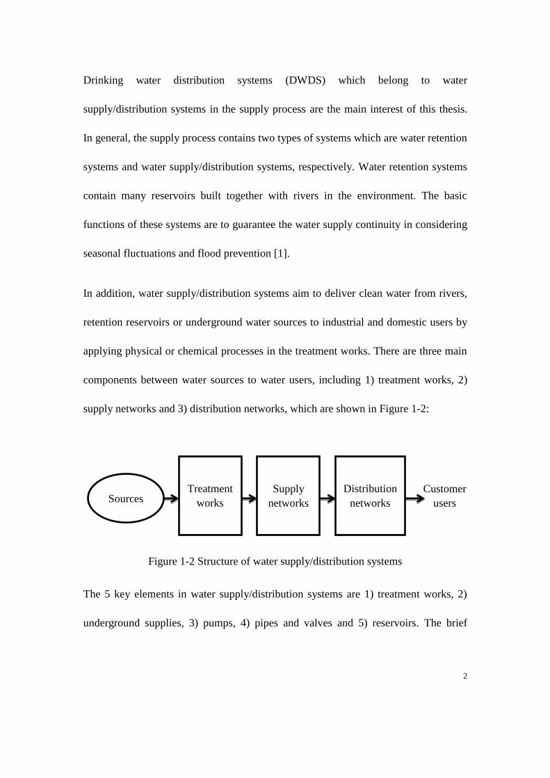
In addition, water supply/distribution systems aim to deliver clean water from rivers,
retention reservoirs or underground water sources to industrial and domestic users by
applying physical or chemical processes in the treatment works. There are three main
components between water sources to water users, including 1) treatment works, 2)
supply networks and 3) distribution networks, which are shown in Figure 1-2:
Figure 1-2 Structure of water supply/distribution systems
The 5 key elements in water supply/distribution systems are 1) treatment works, 2)
underground supplies, 3) pumps, 4) pipes and valves and 5) reservoirs. The brief
Sources Treatment
works
Supply
networks
Distribution
networks
Customer
users
3
descriptions on treatment works and underground supplies are given as follows. The
other elements are to be introduced in Chapter 3.
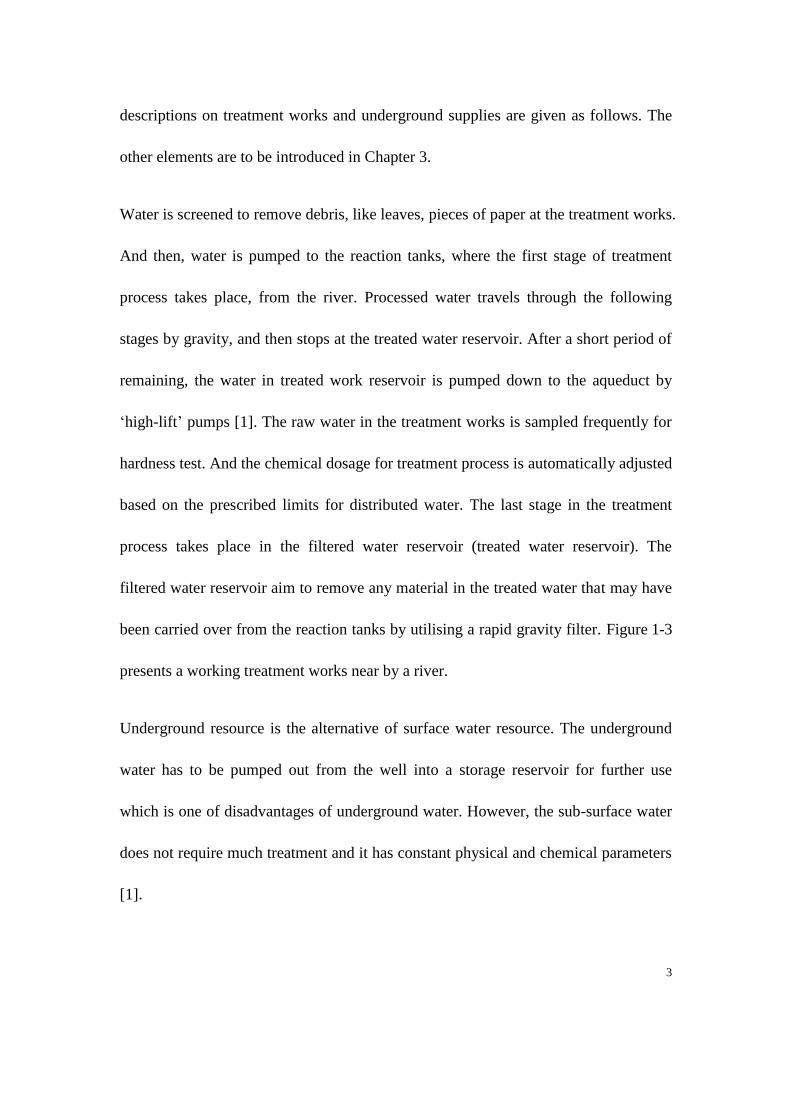
Water is screened to remove debris, like leaves, pieces of paper at the treatment works.
And then, water is pumped to the reaction tanks, where the first stage of treatment
process takes place, from the river. Processed water travels through the following
stages by gravity, and then stops at the treated water reservoir. After a short period of
remaining, the water in treated work reservoir is pumped down to the aqueduct by
‘high-lift’ pumps [1]. The raw water in the treatment works is sampled frequently for
hardness test. And the chemical dosage for treatment process is automatically adjusted
based on the prescribed limits for distributed water. The last stage in the treatment
process takes place in the filtered water reservoir (treated water reservoir). The
filtered water reservoir aim to remove any material in the treated water that may have
been carried over from the reaction tanks by utilising a rapid gravity filter. Figure 1-3
presents a working treatment works near by a river.
Underground resource is the alternative of surface water resource. The underground
water has to be pumped out from the well into a storage reservoir for further use
which is one of disadvantages of underground water. However, the sub-surface water
does not require much treatment and it has constant physical and chemical parameters
[1].
4
River
Stream A Coagulant Stream B Stream C
Sulphur Dioxide
Figure 1-3 Presentation of a treatment works
Although supply systems and distribution systems have the same physical structure,
the feature of these two systems is different and can be summarised as follows [1]:
Screens / Low-lift Pumps
Reaction Tanks
Flash Mixer
Contact Tank
Filters
Filtered Water Reservoir
High-lift Pumps
Aqueduct
Lime
Soda ash
Acid
Chlorine
5
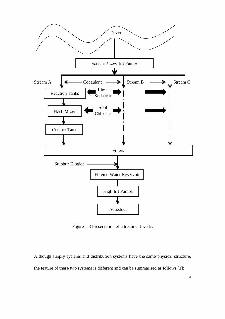
Features of water supply systems:
1. Simple network structure with a limited number of connections;
2. Pipes with large diameter to transport bulk quantities of water;
3. Powerful pump stations composed of many pumps, mostly high-lifting pump;
4. Interactions with the distribution part of the system are modelled as demands
which can be predicted with good accuracy;
5. System flows are insensitive based on reservoir level variations.
Features of water distribution systems:
1. Complicated network structure with hundreds of connections and many loops;
2. A typical zone contains at least one reservoir to sustain supplies and maintain
pressures;
3. Reservoir level variations may have significant impact on the flows and pressures
of the system.
1.1.2 Chlorination of Drinking Water in the Chemical Process
The final stage of treatment at drinking water plant is to kill the bacteria which will
cause waterborne illness is disinfection. However, disinfectant may decay during
transportation in the distribution networks, and the bacteria can grow during water
6
transportation. Although bacteria are reduced by disinfectant in the network, the
re-growth of them may still cause potential problems for water users. Hence, a certain
level of disinfectant concentration is required to prevent bacteria re-growth in
networks. Generally, the method of maintaining disinfectant concentration at a
required level in DWDS is by injecting disinfectants into the network at certain
positions in the network.
There are number of chemical disinfectants that can be utilised in the DWDS,
including chlorine, monochloramine, hypochlorite, chlorine dioxide, chloramines and
ozone. Moreover, non-chemical methods are also considered for disinfecting water,
such as irradiation, anolyte and ultraviolet (UV) [2]. Chlorine is used as a primary
disinfectant in DWDS because of its low cost and effective reduction on a variety of
waterborne pathogens, such as Giardia, Cryptosporidium and viruses [3].
Monochloramine is popularly used as a secondary disinfectant because of its high
efficiency in killing viruses, bacteria and other harmful microorganisms. One
advantage of monochloramine is its chemical stability compared to chlorine, which
makes monochloramine lasting longer in DWDS than chlorine. However, it takes a
much longer time to act with microorganisms than chlorine, which makes
monochloramine an effective secondary disinfectant [4].
7
By adding the chlorine gas to water, the chemical reaction between water and chlorine
can be expressed as [5]:
2 2Cl H O HOCl Cl (1-1)
2HOCl H O H OCl (1-2)
The combination of hypochlorous acid ( HOCl ) and hypochlorite icons ( OCl ) is
called free chlorine, which is determined by the pH. Free chlorine contains
approximately 95% HOCl at pH 6, while it contains approximately 95% OCl at
pH 9 [6]. From the viewpoint of water quality control, maintaining concentration of
free chlorine in the DWDS at a required level is one of the objectives. In general, a
minimum concentration of free chlorine is needed for controlling the hazardous
microorganisms in drinking water. Moreover, a value of 0.2 mg/L is determined by
the Environment Protection Agency of United States (U.S.EPA) in practice [2].
1.1.3 Disinfection by Products
In the 1970s, existence of disinfection by-products (DBPs) was observed during the
water treatment process because chlorine reacts with the organic matters that exist in
the bulk water or pipe walls. Health-dangerous DPBs are considered the carcinogenic
matter in drinking water systems. A number of DBPs have been identified after
8
discovering Trihalomathanes (TTHM). The reaction kinetics of producing DBPs can
be found in [6-8].
Many countries have proposed several regulations for water treatment processes and
the operation of DWDS for controlling the potential health hazards from DBPs. The
EPA made a two-stage regulation on disinfectants and DBPs called Disinfectants and
Disinfection Byproducts Rules (DBPR). The stage 1 DBPR aims to reduce drinking
water exposure to DBPs. It is applied to drinking water systems that inject disinfectant
into the drinking water during the treatment process. And the stage 2 DBPR
emphasise on enhancing public health protection by tightening monitoring
requirements on TTHM and Haloacetic acides (HAA5). The final stage 1 DBPR
includes the following regulations [3]:
Maximum residual disinfectants level goals (MRDLGs):
1. Chlorine (4 mg/L)
2. Chloramines (4 mg/L)
3. Chlorine dioxide (0.8 mg/L)
Maximum contaminant level goals (MCLGs):
1. Three trihalomethanes:
(a). Bromodichloromethane (zero)
(b). Dibromochloromethane (0.06 mg/L)
(c). Bromoform (zero)
9
2. Two haloacetic acids:
(a). Dichloroacetic acid (zero)
(b). Trichloroacetic acid (0.3 mg/L)
3. Bromate (zero)
4. Chlorite (0.8 mg/L)
MRDLs for three disinfectants:
1. Chlorine (4.0 mg/L)
2. Chloramines (4.0 mg/L)
3. Chlorine dioxide (0.8 mg/L)
MCLs:
1. For total trihalomethanes (0.080 mg/L): a sum of the three listed
above plus chloroform,
2. Haloacetic acids (HAA5) (0.060 mg/L): a sum of the two listed
above plus monochloroacetic acid and mono- and dibromoacetic
acids
3. Two inorganic disinfection byproducts:
(a). Chlorite (0.1 mg/L)
(b). Bromate (0.010 mg/L)
A treatment technique for removal of DBP precursor material.
10
Note that the zero MCLG for chloroform has been removed by the EPA from its
National Primary Drinking Water Regulations [2].
1.1.4 Advanced Water Quality Control Algorithm-Model Predictive Control
After two quality objectives introduced in the previous two sections, an advanced
control technology is required to control the two water quality objectives. The main
concern of controller-designer is to meet the prescribed requirements of a given target
system under different constraints. However, systems can be classified into different
categories, such as linear or non-linear, small scale or large scale. In reality, the target
systems are nonlinear, constrained with multi-variables. Therefore, an advanced
control algorithm is needed based on the characteristics of target systems.
In this research, the designed controller needs to handle two objectives with specified
constraints, which are free chlorine and DBPs, respectively. For free chlorine, the
concentration of free chlorine at monitored nodes must be maintained within defined
lower and upper limits. And in terms of DBPs, the concentration of DBPs at
monitored nodes has to be kept as lower as possible. Let us consider the standard
controller first, for example, PI controller. PI controller is utilised for tracking the
defined reference for plant outputs, and it is suitable for linear systems, especially for
single output single input systems. In this research, there is no output reference to
11
track but a reference zone to maintain and a minimisation task. Therefore, the
standard controllers are not suitable to handle this nonlinear system with
multi-outputs when no reference provided, especially for the case that there are
interactions between the outputs.
In this thesis, Model Predictive Control (MPC) is selected as the main control strategy
to handle the nonlinear, constrained with multivariable problems in water quality
control of DWDS. The basic principle of MPC is that MPC repetitively solves the
optimisation problems on-line over the defined output prediction horizon.
The MPC algorithm repeats at every MPC control time step by updating the measured
or estimated plant states into the model of the plant. This receding horizon algorithm
can handle time-varying disturbance or constraints since the model is initialised at
every step by taking the feedback from the plant and only the first action of optimised
control sequences is utilised for the plant.
Application of MPC on DWDS has been investigated in previous research on water
quality control but with a linear quality dynamic model. In this thesis, MPC is applied
on a nonlinear water quality dynamic model which considers the dynamic of DBPs.
12
1.1.5 Motivations
Drinking water is considered a rare resource in the world, especially in developing
countries. It has a significant impact on people’s daily life, especially on the health of
those living in a developing area. However, water systems are complex because of
their nonlinearity and unknown disturbance when operating in reality.
Water quality control is one of the main topics in DWDS. Based on the discovery of
scientists in recent years, people have drawn much attention to carcinogenic materials
brought by DBPs. Presently, the carcinogenic mechanism brought by DBPs is still
under investigation. Therefore, controlling disinfectants and DBPs in DWDS becomes
a hot topic in this field. In practice, the applications of water quality control in water
industries are based on the water quality concentration measurements by employing
data analyser suck as colorimeter, spectrophotometers and portable equipment. The
dosage of chlorine gas is determined by analysing the data collected at monitored
positions and highly-qualified personnel experience [9, 10]. Besides, the previous
researches on analysing water quality control are based on the linear water quality
model which only considers dynamic of chlorine. The generation of DBPs in water
quality dynamics makes the water quality control problem much more complicated
because the dynamics become nonlinear and more objectives are involved. Hence,
jointly control of DBPs and free chlorine in DWDS requires advanced control
technology.
13
Although much work has been done to address the water quality control problem,
research work on the consideration of DBPs still needs to be enhanced. For example,
the water quality dynamic model is not linear anymore which means a new control
mechanism is needed. Therefore, it is worthwhile to carry out studies on such
nonlinear water quality models from the aspect of its characteristic of nonlinear
dynamics, modelling in parameters with uncertainty, monitoring the disinfectants and
DBPs in the DWDS.
The motivations of conducting this research can be summarised as follows:
1. Safety of limited drinking water resource has been draw people’s great attention
on daily use, especially after discovery of health-dangerous DBPs.
2. The measurement equipment employed in practice is expensive, and the
high-qualified personnel experience is also difficult to achieve. Therefore, it is
necessary to investigate intelligent control methods to meet water quality control
objectives.
3. As explained in the previous section, when compare to the standard controller,
such as PI controller, MPC control algorithm is suitable to handle the nonlinear
multivariable system with input-output constraints.
14
1.2 Aims and Objectives
This thesis aim to control the dynamic of both chlorine and DBPs in a proper way
based on the newly derived nonlinear water quality model [7] that 1) free chlorine can
be maintained within the prescribed limits so that the bacteria re-growth is halted in
the whole DWDS, and 2) the potential hazards brought by cancerigenic matter DBPs
can be dramatically reduced.
In reality, chlorine should not be the only objective considered in the water quality
control problem. The cancerigenic objective DBPs is also required to be taken into
consideration for decreasing the potential hazards in drinking water systems. In this
thesis, the objective and sub-objectives of controlling water quality with considering
DBPs can be summarised as follows.
1. The nonlinear MPC controller is to be designed.
(a). The model of the plant is modelling based on a simulator at this stage, which
is EPANET simulator that is widely used in generating hydraulic and quality
data. However, EPANET is only used for simulating linear water quality
models which means only disinfectant data is to be generated. Therefore, the
Multi-Species Extension of EPANET (EPANET-MSX) is required for adding
DBPs into the simulator.
(b). In general, the modelling horizon for DWDS is set to 24 hours. The size of
15
control horizon and output prediction horizon for the MPC controller are
needed. Determination of these two time horizons is based on the quality
control performance. In order to observe the influence caused by inputs, the
control horizon must not be longer than the prediction horizon since
detention time generated by water transportation. Setting a shorter controller
horizon could reduce the computation time at each MPC time step, but
efficiency of MPC controller will decrease as well because more MPC
control steps are needed. Increasing controller horizon could observe more
quality outputs and reducing the impact brought by transfer delay, however,
the computation increases dramatically. Therefore, determining control
horizon and output prediction horizon properly is a challenge in water quality
control.
(c). A further problem in designing the MPC controller is to select a proper
optimisation solver and define the objective function for the MPC controller.
The selection is based on the characteristics of the defined objective function
and behaviour of DWDS. Performance of such optimization solver requires
analysis. Can DBPs be controlled by a defined optimisation problem? What
difference can be observed between the linear water quality model and the
nonlinear water quality model? Whether these questions can be solved
theoretically has to be answered by analysing the simulation results.
16
(d). Tuning parameters of reaction kinetics in quality dynamics for obtaining a
better performance.
2. Taking the uncertainty into consideration when the nonlinear water quality model
is used.
(a). Linearization is commonly used in dealing with nonlinear problems but
creates another problem which is structure error caused by linearization.
Select a proper way to implement linearization of nonlinear water quality
model is an important part of modelling.
(b). Bounding approach is a general way to handle unknown parameters of model.
Once the model considering uncertainty is accomplished, bounding chlorine
and DBPs separately or jointly is the other problem need to be solved.
(c). Validation on the completed model is needed for verifying its accuracy.
(d). Robustly predicting outputs of obtained model is one of main challenges in
this research.
(e). Simulating the accomplished model and analysing the simulation results are
essential to describe the performance of obtained model with considering
uncertainty.
17
1.3 Contributions
The main contributions of this thesis can be summarised as follows:
In the previous research on optimising water quality control, only the dynamic of
disinfection is considered in the linear water quality model. The thesis has
developed the nonlinear MPC controller for controlling water quality in DWDS
based on the advanced nonlinear water quality dynamic model which jointly
considers disinfection and DBPs objectives.
The quantity in DWDS operates at a slow dynamic time scale measured in hours
while quality operates in a fast dynamic time scale measured in minutes. The two
different time-scale operation makes optimsing control on water quality much
more complicated. The developed nonlinear MPC controller has been
demonstrated its capability on handling highly nonlinear, constrained with
multivariable and multi time-scale systems.
In the previous research, the chlorine and DBPs were controlled independently
and the interaction between chlorine and DBPs is ignored. In this thesis, the
interaction between chlorine (disinfection) and DBPs are considered and jointly
controlled under their dependent constraints within the developed nonlinear MPC
controller.
In the previous research, the PPM is applied to handle the uncertainty and
structure error in water quality model. However, only the multi-input
18
single-output (MISO) PPM framework is obtained and only the parameters of
chlorine (disinfection) are bounded and estimated. In this thesis, the multi-input
multi-output (MIMO) model structure on nonlinear dynamic water quality model
considering DBPs has been derived and presented. The parameters explaining
dynamics of chlorine and DBPs are jointly bounded and estimated. And the
outputs, including both chlorine and DBPs, are predicted robustly.
The output prediction algorithm has been modified to incorporate the MIMO
model in order to robustly estimate the parameters of the nonlinear quality model
within the augmented objective-DBPs.
In previous research, the PPM is applied to linear water quality model. In this
thesis, an advanced nonlinear water quality model is applied to derive the MIMO
PPM. The capability of the PPM in appropriately processing nonlinear systems
optimisation problems has been proved by simulation results.
1.4 Thesis Outlines
Based on the above research focuses, the content of each chapter is summarised as
follows:
Chapter 2: A literature review concerning existing research on operational control of
DWDS is presented. The corresponding reviews on water quality control and MPC
19
control mechanisms are presented in detail. The literature on introducing GA is also
presented.
Chapter 3: The fundamentals of operational control in DWDS are presented. The
physical elements in DWDS are introduced and their operational laws are presented in
detail. Fundamentals, physical components and the related operation laws are to be
employed in the simulated DWDS network utilised in Chapter 4 and Chapter 5. The
path analysis algorithm is explained. And the application of path analysis algorithm is
presented in Chapter 5.
Chapter 4: This chapter introduces the two time-scale hierarchical structure in DWDS
which integrates quantity and quality. A newly derived nonlinear water quality model
is presented. The MPC controller for jointly controlling chlorine and DBPs under
input and output constraints is designed and presented. Application of such MPC
controller to a case study DWDS network is presented in detail.
Chapter 5: Because the uncertainty is not considered in EPANET and EAPENT-MSX
simulators, an advanced nonlinear water quality model with uncertainty is required.
Therefore, PPM is introduced in this chapter. The MIMO structure for jointly
bounding chlorine and DBPs is presented for the first time. The experiment design on
obtaining the PPM is explained in detail. The algorithm for obtaining piece-wise

20
constant parameters is presented. The modified robust output prediction algorithm is
also presented in this chapter.
Chapter 6: The research work of this thesis is concluded in this chapter, together with a
presentation of the further research topics.
21
CHAPTER 2 LITERATURE REVIEW
Model predictive control for water quality in drinking water distribution system that
considers the impact of disinfectant by-products is a new topic in the water quality
control field. Lots of literature has contributed to this research topic.
The review conducted in this chapter is carried out under the following aspects: 1)
operation control on drinking water distribution systems including chlorine residual
control, overview of disinfection by-products, placement of booster stations and
monitoring sensors; 2) overview of model predictive control, including linear and
nonlinear MPC, robust MPC, and optimisation improvement in MPC.
2.1 Overview of Operational Control on Drinking Water
Distribution Systems
Drinking water distribution systems (DWDS) have been the subject of research for
many years in order to guarantee the safe delivery of drinking water [11]. DWDS are
groups of large scale complex networks containing water reservoirs (part of a water
resource), storage tanks, pumps, valves and pipes which distributed across the whole
network and connected with each network component to deliver safe water to the user’s
taps [2]. In order to supply high quality water to customers and satisfy consumers’
22
demand in terms of both quantity and quality, implementation of the operational
control of DWDS is necessary [2].
Quantity and quality are the two major aspects in the operational control of DWDS.
The main objective of quantity control is handling the flow of pipes and pressures at
the network junction nodes by producing optimal control schedules on valves and
pumps, so that the customer water demand is satisfied and the electrical energy cost
cause by pumping is minimised [1, 12].
In the other hand, maintaining the free disinfectant concentration at the monitored
nodes (selected based on the characteristic of target DWDS) within the prescribed
limits, including upper and lower limits, in such a way that the bacterial re-growth
over a whole DWDS is halted is the main objective of water quality control [13].
However, as the free disinfectant reacts with the organic matter during the
transportation over the DWDS producing so called disinfectant by-products (DBPs),
which are dangerous to health, the DBPs concentration level over the DWDS are
required to be as low as possible [14]. Minimising DBPs concentration at monitored
nodes is considered as another objective of the water quality control in DWDS [13].
This augmented objective has enriched the objective in water quality control, and
made the water quality control more complicated.
There is interaction between quality and quantity although it is a one way interaction
from quantity to quality [13]. “Water quality is significantly determined by water
quantity” this implies that in order to obtain a desirable water quality, controlling
water quantity is a necessary step [15]. This feature makes it impossible to control
23
quality or quantity without support from the other aspect. Therefore, an integrated
manner for controlling both quantity and quality is needed.
However, due to different time scales in the internal dynamics of the hydraulic and
quality, which can be described as slow and fast, respectively, a dimension
complexity of the integrated control task becomes large. This makes the direct
application of integrated control on water quality and quantity impossible, even for a
small size DWDS [16].
To solve such problem, a hierarchical two time-scale control structure was proposed
in[17, 18]. The basis of the control structure consists of two levels: Upper Control
Level (UCL) and Lower Correction Level (LCL). Each level has its own optimising
controller. The controller at the UCL operates on a slow hydraulic time (e.g. our hour)
scale based on the accurate hydraulic model and simplified water quality model with
the same time step (e.g. one hour). The models in UCL are used to predict the
quantity and quality controlled outputs over the hydraulic prediction horizon (e.g. 24
hours). At the beginning of a control period, states of water quantity and quality,
including 1) water flows, 2) pressures and 3) disinfectant concentrations at junction
nodes or distributed in pipes are measured or estimated, and then sent to the integrated
quantity and quality optimiser. Moreover, the prediction of water demand is also
provided to the optimiser.
Due to the one-way interaction between quantity and quality, the hydraulic controls
resulting from solving the optimisation task in UCL are truly optimal. The quality
dynamics model in this optimisation problem has the same time step to the quantity
24
dynamic model. Although the dimension of the optimisation problem is decreased, the
modelling error of water quality dynamic is increased.
Therefore, improvement on the quality model is needed and this can be done at the
LCL by applying the fast quality feedback controller which operates at a faster quality
time scale (e.g. 5 minutes). The flows, considered as one of the quality controlled
inputs and required at the LCL by the fast quality controller, are determined at the
UCL.
There are several essential problems contained in the operational control of DWDS,
which include 1) water quantity control, 2) water quality control, and 3) integrated
control on both quantity and quality, 4) placement of hard sensors and booster stations
and 5) soft monitors design. Literature related to these topics will be critically
reviewed in the following sections.
2.1.1 Review on Quantity Control in Drinking Water Distribution Systems
The optimisation problem on quantity control considered by UCL includes 1)
optimising the operation schedule of pumps and storage facilities, 2) minimising the
energy cost and 3) optimising the valve and flow schedules.
According to the least cost design problem of DWDS proposed in [19-21], optimising
pump operation becomes a hot topic in the field of managing DWDS [22]. Various
methods have been developed to solve this problem since 1970 when dynamic
programming (DP) was employed in [23] and [24] for energy saving optimisation. The
25
results analysed in [24] has been shown that a conventional dynamic programming
method can be applied to a simple DWDS. The total pumping costs can be evaluated
accurately by taking account of factors including reservoir constraints, pumping
efficiency, maximum demand tariffs and so on. Generally, DP can be used to solve
some complex optimisation problems by breaking these problems into several simpler
sub-problems, and solving each of the sub-problems and storing their solutions by
utilising a memory which is data based structure. DP examines the previously solved
sub-problems and combines their solutions to generate the best solution for the
succeeding problems. However, DP is limited on solving those optimisation problems
composed of unsolvable sub-problems or parametrised independently sub-problems.
Different from DP, the linear programming (LP) procedure was utilised as the core of
the developed planning model to deal with the pump operation problem in large-scale
DWDS with a directed graph algorithm [25]. The results have been shown that the
combination of LP and directed graph algorithm provides an extremely versatile tool to
assist in the planning and management of a large-scale DWDS. Although LP is widely
used, the linear assumption is a key weakness which limits its application.
Model predictive control (MPC) with genetic optimisation solver and adaptive
multi-objective MPC were implemented in [26] and [27], respectively, for providing
the optimal solution of quantity control in DWDS. Both of them are based on MPC
driver but with different type of objective functions. Quantity optimisation problems
were combined with quality optimisation in [26], while [27] solved the quantity
optimisation problems independently as form of multi-objectives. However, the
computation in [26] is more time-demanding compared to that in [27]. Other methods,
26
such as nonlinear programming (NP) [28, 29], mixed-integer [30, 31] and
metamodeling [32, 33] also performed well in providing proper solutions for quantity
operation optimisation. Different methods applied are based on the characteristic of
defined objective function or the purpose of solving described problems. For example,
mixed-integer can be utilised in [30] because the gradients of objective function were
known so that sequential quadratic programming (SQP) was applied for solving the
optimisation task. And metamodeling was employed in [32] due to the purpose of
reducing the computation time in solving the control optimisation problem in DWDS
which means developing on modelling is significant. The further developed robustly
feasible model predictive control (RFMPC) approach has been applied to quantity
control in DWDS in [34] for solving the online optimising control problem in nonlinear
plants with output constraints under uncertainty. Compared to normal MPC approach,
RFMPC is more reliable and feasible in handling the uncertainty of control
optimisation problems in DWDS.
2.1.2 Review on Chlorine Residual Control in Drinking Water Distribution
Systems
Water is an important resource for both industrial and domestic usage [2]. However,
due to climate change, a rising population and environment pollution, an increasing
shortage of natural water resources around the world has been observed [35, 36]. This
makes the protection of drinking water more important.
27
Drinking water is transported by DWDS from the water plant to consumer taps. As a
result, meeting the demand for drinking water within the prescribed quality limits
requires advanced control technology to operate DWDS. The advanced control
technologies are discussed in this thesis. As mentioned above, quality control is
divided into two parts: maintaining chlorine residual concentration throughout the
whole water network within the prescribed limits, and keeping the concentration of
disinfectant by-products as low as possible since disinfectant by-products are
dangerous to health [13].
Modelling the quality model in a proper way is essential for achieving the quality
control purpose. The previous research on water quality control mainly focused on a
linear quality model. It means that chlorine residual is the only target to be maintained
within the limits or minimised based on specified objectives.
A mass-transfer-based model was proposed in [37] for predicting chlorine decay in
DWDS. The first-order reactions of chlorine occurring in the bulk flow and at the pipe
wall are considered in this model. It is capable to explain the observed phenomena
during the process of chlorine decay. However, all pipes in a network use the single
wall decay would not be suitable for DWDS. In [6], a second-order kinetics model has
been developed for better describing the chlorine decay and explaining the
relationship between chlorine decay and the impact caused by bulk flow and the pipe
wall.
28
In terms of controlling water quality at the monitored nodes in DWDS, a robust model
predictive controller has been developed in [38] to maintain chlorine residuals within
the prescribed upper and lower limits based on a state-space water quality model. The
comparison between input-output modelling and state-space modelling regarding
chlorine residuals control in DWDS has been presented in [2]. Compared to the result
obtained from input-output modelling, that obtained from state-space modelling has
been shown a more smooth performance. However, the computation time in
state-space modelling is much more than that in input-output modelling.
Control of an uncertain time-varying linear dynamical system with deferred inputs has
been achieved in [39]. The disturbance inputs, model parameters and the model
structure errors of these systems are totally unknown. However, the inputs, parameters
and structure errors can be bounded in an appropriate way. The output constraints are
regulated by employing a model based predictive controller which uses a set of
bounded uncertainties and appropriate safety zone design. This regulating method
simplified the calculation on searching unknown parameters with limited information.
And the designed safety zone guaranteed satisfaction on output constraints. However,
feasible solutions may not be existed with obtained safety zone which requires a
further investigation on the safety zone design approach.
The further developed intelligent model predictive controller is proposed in [40] for
maintaining the bounding limits of chlorine residuals under uncertainty caused by
29
modelling and demand prediction, and also under control input constraints. The
quality feedback controller has been designed to implement the linear quality control,
and the model parameter estimation and model output prediction have been achieved
by utilising the set-bounded modelling of an uncertainty. The further developed robust
MPC controller is more feasible than previous one as the constraints of input are
considered in this controller.
Apart from applying model predictive control technology, the decentralised model
reference adaptive control is implemented to control water quality in water
distribution networks in [41], and the further developed adaptive control formulation
to maintain chlorine residuals in DWDS is proposed in [42]. The adaptive control
approach and related formulation are based on approximation of the input or output
dynamic behaviour of chlorine in DWDS. The approximated dynamic behaviour is
considered as the discrete linear time-varying model with unknown parameters. The
foundation of adaptive control is parameter estimation which makes adaptive control
popular especially in solving the optimisation problem with known varying
parameters, or initially unknown parameters. However, MPC algorithm is not adept at
solving problems unknown parameters independently. Combination of adaptive
control and MPC may able to provide a reliable and feasible solution for these
highly-nonlinear, multi-constrained with unknown parameters control optimisation
problems.
30
2.1.3 Review on Disinfectant by-Products: History, Formation, Regulation
and Control
Trihalomethanes (TTHMs) were the first class of halogenated DBPs identified in
chlorinated drinking water [43, 44]. And the coincided related findings highlighted
the link between the cancer and consumption on chlorinated water [45]. The National
Organics Reconnaissance Survey conducted in 1975 by the U.S. Environmental
Protection Agency (EPA) found that chloroform caused by chlorination was
ubiquitous in all chlorinated water [46].
The National Cancer Institute identified chloroform as a carcinogen in 1976 [47].
Therefore, the EPA defined the limits of TTHMs [48] in drinking water. The
maximum contaminant level (MCL) of total TTHMs was 0.1 mg/L. After identifying
the existence of TTHMs in chlorinated finished drinking water, it was then discovered
that only TTHMs were produced in the chlorination process.
Dichloroacetic acid and trichloroacetic acid were identified and known as the second
class of DBPs in chlorinated drinking water [49-53]. Asides the halogenated DBPs
mentioned above, there were other identified halogenated DBPs, such as 1) chloral
hydrate, 2) haloacetonitriles, 3) chloropicrin, 4) haloketones, and 5) cyanogen
chloride. These DBPs are of a lower concentration (compared to TTHMs) however
31
still have effects on human health[54]. In order to investigate the adverse health
effects associated with these specified halogenated DBPs, so many epidemiological
researches have been developed since 1974. A feeble link between chlorinated water
and cancers, such as bladder, colon and rectal cancer, has been gradually found in
these researches [54, 55].
To achieve the required 0.1 mg/L MCL of TTHMs, water supply industries have
adopted various strategies to comply with the new regulation. The most common
treatments include: 1) moving chlorination downstream point into the treatment train,
2) reducing the chlorine doses and 3) employing an alternative disinfectant like
chloramines to replace free chlorine [56]. The second treatment is the safest way to
achieve the required MCL of TTHMs but with the worst performance, because
reducing the chlorine doses may also reduce the chlorine concentration at remote
junction nodes lower than minimum requirement. The third treatment is not
recommended in normal case as chloramine is danger to use than chlorine.
Although new modifications mentioned above have shown that the target MCL for
TTHMs could be achieved at an acceptable cost, problems about the impact of these
modifications were raised, such as whether the microbial quality of finished drinking
water was compromised as a result of these modifications [45]. The Surface Water
Treatment Rule (SWTR) and the Total Coliform Rule (TCR) was published by the
U.S.EPA in 1989. The rules above aim to 1) guarantee the microbial quality of treated
32
water was not compromised, and 2) address the concerns on waterborne diseases/viral
diseases [57, 58].
The EPA has tried a number of methods to balance the risk brought by DBPs and
microbial disease [59]. However, the uncertainty on health effects and other
promiscuous factors have made the EPA continue a negotiated rule-making method
for appropriately regulating DBPs in drinking water [60].
According to the recent research on water quality control, chlorine residue is not the
only objective any more. The prediction of chlorine residuals in DWDS is now taking
the effect of disinfectant by-products into consideration [13]. This makes the linear
water quality model become nonlinear. The augmented DBPs objective makes the
water quality control problem more complicated.
Since the 1970s, the research on drinking water has mainly focused on understanding
the occurrence of DBPs in chlorinated drinking water [61]. The interest on the
developed models which applied to estimate the formation and the impact of DBPs
has grown during recent years. This is because of the potential association of DBPs
with cancer, particularly bladder and rectal cancer [54, 55].
The disinfection process starts at the beginning of the 20th century to inactivate and
eliminate the pathogens in DWDS [61, 62]. The disinfection process in DWDS
reduces the microbial risks, but simultaneously results in a chemical risk caused by
33
DBPs. DBPs are by-products of the disinfection process. They are produced by the
reaction of disinfectant and the natural organic matter (NOM) and/or inorganic
matters existed in DWDS.
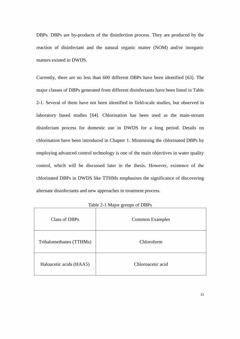
Currently, there are no less than 600 different DBPs have been identified [63]. The
major classes of DBPs generated from different disinfectants have been listed in Table
2-1. Several of them have not been identified in field-scale studies, but observed in
laboratory based studies [64]. Chlorination has been used as the main-stream
disinfectant process for domestic use in DWDS for a long period. Details on
chlorination have been introduced in Chapter 1. Minimising the chlorinated DBPs by
employing advanced control technology is one of the main objectives in water quality
control, which will be discussed later in the thesis. However, existence of the
chlorinated DBPs in DWDS like TTHMs emphasises the significance of discovering
alternate disinfectants and new approaches in treatment process.
Table 2-1 Major groups of DBPs
Class of DBPs Common Examples
Trihalomethanes (TTHMs) Chloroform
Haloacetic acids (HAA5) Chloroacetic acid
34
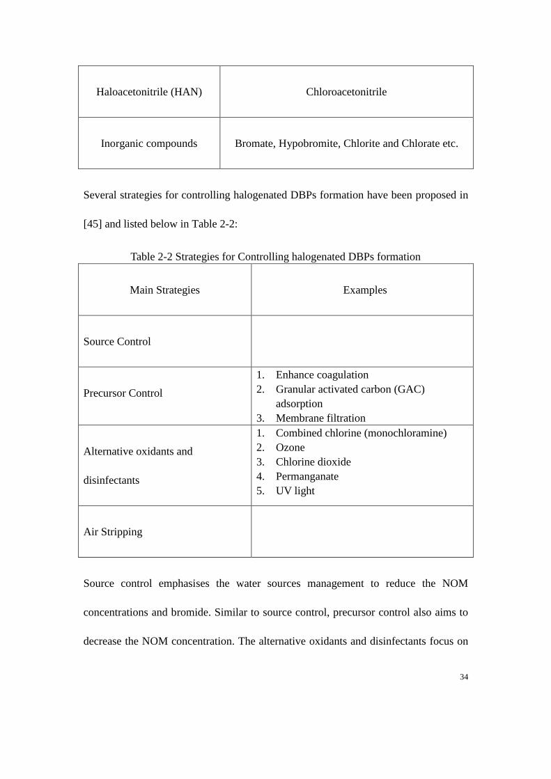
Haloacetonitrile (HAN) Chloroacetonitrile
Inorganic compounds Bromate, Hypobromite, Chlorite and Chlorate etc.
Several strategies for controlling halogenated DBPs formation have been proposed in
[45] and listed below in Table 2-2:
Table 2-2 Strategies for Controlling halogenated DBPs formation
Main Strategies Examples
Source Control
Precursor Control
1. Enhance coagulation
2. Granular activated carbon (GAC)
adsorption
3. Membrane filtration
Alternative oxidants and
disinfectants
1. Combined chlorine (monochloramine)
2. Ozone
3. Chlorine dioxide
4. Permanganate
5. UV light
Air Stripping
Source control emphasises the water sources management to reduce the NOM
concentrations and bromide. Similar to source control, precursor control also aims to
decrease the NOM concentration. The alternative oxidants and disinfectants focus on
35
supplementing or replacing the chlorination process. Air stripping moves air through
contaminated groundwater or surface water into an above-ground treatment system.
However, the removed chemicals called ‘Volatile Organic Compounds’ are easily
evaporated. This danger characteristic makes air stripping not recommended as a
desirable treatment strategy.
2.1.4 Integrated Control of Both Quality and Quantity in DWDS
As described in previous section, quantity and quality are the two major aspects in
control of DWDS with observed interactions. For the purpose of satisfying the
quantity-quality interaction, [65-68] developed several proposals for considering both
quantity and quality into one integrated control scheme. [65, 66] have implemented
optimal operation control of a multi-quality supply/distribution system under different
hydraulic conditions, steady-state flow and unsteady conditions, respectively. Results
analysed in these two literatures have demonstrated that optimal operation of
integrated quantity and quality control can be formulated and solved. But, they are
limited to small-size networks because large-size networks make the formulation of
optimisation problem much more difficult, even impossible to be formulated. In order
to transfer the real-measured data into the integrated online-solved optimisation
problems, receding horizon control technology was proposed in [67]. This control
36
scheme provided a possible strategy to solve the integrated control problem on-line.
[68] has employed the NP to solve the optimal pumping schedule problem
considering water quality. However, the optimal solution obtained from the proposed
methodology cannot be applied in practise because the optimal solution is local
optimal, not global optimal.
Minimising the operational cost, satisfying the water demand with required quality
and maintaining multi-constraints on quantity and quality are the main objectives in
the optimising integrated control of water quality and quantity in DWDS [17, 69]. The
constrained optimisation problems are complex because of following reasons: 1)
nonlinearities, 2) large dimension, 3) output constraints, 4) mixed-integer structure of
the involved variables, and 5) two time-scale dynamics in the system [16, 18].
An integrated approach named as the hierarchical control has been proposed in [17,
18, 69], where a hierarchical two-level structure was applied for incorporating the
defined controller objective functions and making the synthesis of them possible. A
feedback optimisation control in DWDS has been proposed in [70] with the
optimising model predictive controller to overcome the integrated quantity and quality
control problem. The proposed hierarchical structure uses two independent
optimisation solvers for each control level because two time-scales of dynamics
existed in quantity and quality. However, the feedback optimisation control built a
37
link between two independent optimisation solvers and made interaction between two
independent optimisation solvers possible.
2.1.5 Placement of Booster Stations and Hard Sensors in Drinking Water
Distribution Systems
The treatment plant controls chlorine residuals directly to ensure the water entering
into the entire DWDS compiles with the related standards. However, during the water
transportation throughout the whole network, the free chlorine consumes bacteria and
reacts with NOM. This will result in major decay and generation of DBPs,
respectively. Thus the water safety may not be guaranteed especially at those remote
junction nodes for domestic users. It is necessary to inject free chlorine by employing
booster stations located at appropriate junction nodes of DWDS.
Booster disinfection is the additional disinfectant located at certain specified point
distributed throughout a DWDS. It is used to ensure that the disinfectant residuals in
DWDS are greater than the minimum amount [71]. Booster disinfection reduces the
disinfectant dose amount compared to the conventional methods that use disinfectant
only at the water source [71]. Such booster disinfections can reduce the mass of
disinfectant and maintain a detectable residue at consumption junctions around the
38
distributed network, which could lead to decreased formation of disinfectant
by-products[72].
The problem of allocating disinfectant booster stations so that the amount of dosage
required can be minimised and residuals concentration throughout the DWDS can be
maintained at a required level is presented in [73]. The booster disinfectant location
model involved is formulated by mixed integer linear programming. Although the
results have been shown that the booster disinfectant location model can be applied to
real-scale network, the solution efficiency is lack of validation. Furthermore, the
booster station locations and related injection scheduling problem are discussed in [71]
where a formulated multi-objective optimisation model was proposed. The objectives
of the proposed optimisation model are: 1) minimisation of the total disinfection
dosage, and 2) maximisation of the volumetric demand within prescribed limits.
Multi-objective genetic algorithms were utilised for solving the optimisation problems.
Moreover, a parallel multi-objective genetic algorithm was applied in [74] for
optimising the allocations of booster disinfection in DWDS. Compare the three
methods descried above, the problem considered in [74] is more comprehensive
which makes the approach of parallel multi-objective genetic algorithm more reliable
and realistic.
However, the quality model utilised above is linear and only takes chlorine residue
into consideration. With further development on water quality model, a nonlinear
39
water quality dynamic model which takes DBPs into consideration is proposed in [7].
The optimisation problem of locating disinfectant booster stations requires a new
approach for dealing with the new water quality model.
The optimised allocation of disinfectant booster stations has been addressed in [75]
based on linear and nonlinear water quality models for determining the impact of
different model structures. The allocation task was also formulated as multi-objective
but with both nonlinear and linear mixed-integer optimisation problems. Determining
the allocation of disinfectant booster stations is one of the key issues in implementing
quality control, and the placement of sensors on monitoring water quality is also
important in this field.
The Safe Drinking Water Act requires that the water quality of drinking water in
DWDS is to be sampled at certain locations where can represent the quality status of
the whole distribution networks [76], however, the act does not explain how to select
these sampling locations. Moreover, residual concentration is not the only objective
that requires sampling and monitoring, contamination in drinking water distribution
systems require hard sensors for monitoring as well.
Therefore, Contamination Warning Systems (CWSs) are introduced as a promising
technology for reducing contamination risks in DWDS [77]. The critical problem in
designing a working CWS is to develop the strategies on placing online sensors that
40
can rapidly detect contaminations [77]. Approaches of locating monitoring stations in
a DWDS are first presented in [76] by solving formulated integer programming
problems. The synthesis of coverage matrices, integer programming and pathway
analysis provides a first step towards appropriate algorithms for locating monitors in
DWDS.
With further investigation into the sensor placement problem, several sensor
placement strategies were explored. 1) Expert opinion is the strategies that guided by
human judgment, its reliability is based on people’s experience and expertise
accumulated during solving related tasks in the past. For example, [78] and [79]
evaluated sensor placements by experts who did not use computational models to
determine the best sensor locations. 2) The ranking method is a similar further
approach that aims to use expert information to rank potential locations for
monitoring sensors [80-82]. 3) Formulating the task of sensor placement as an
optimisation problem is the most popular strategy to use so that the performance of a
possible sensor placement can be estimated computationally. Formulating a
optimisation problem is more reliable than the other two strategies especially in some
complicated networks, because calculation on optimisation problem is always stable
and reliable when the formulation is correct while mistakes could be made from
people’s previous experience.
41
There has been a lot of research on sensor placement for DWDS in the past several
years, it is impossible to review all of them, but their valuable research contributes to
the development on controlling water quality in DWDS.
2.1.6 Monitoring by Soft Sensors on Water Quality in DWDS
For implementing MPC control on water quality in DWDS, the quality state feedback
is essential to update at each control time step which means the proper on-line
monitoring system for water quality is required.
Only few DWDS states which include concentrations of chemical and biological
components can be measured on-line by hard sensors located at specified positions in
DWDS due to the sensor access problems, the limit on costs and maintenance [7, 83].
Therefore, the missing information has to be collected by soft sensors which gather
the variable measurements and mathematical models of quality states into water
quality state estimators [7].
Several approaches were developed for achieving the robustness of estimates,
including a set-member ship approach [84, 85], optimisation based set-membership
algorithms [86, 87], cooperative dynamics [88] and interval observers and the interval
state estimation [89-92]. Compared to the follow two methods, the first two methods
are limited to on-line estimation because of the large demand on computation.
42
In the previous research [18, 69, 93, 94], a free chlorine concentration was utilised for
the assessment of water quality state. The recent research work from [13] takes the
additional quality state DBPs into consideration by applying a nonlinear dynamic
water quality model derived based on the work presented in [6, 8, 95]. And
monitoring water quality in DWDS by applying the derived nonlinear water quality
model is addressed in [7].
2.2 Model Predictive Control Overview
Model Predictive Control (MPC), also known as Receding Horizon Control and
Moving Horizon Optimal Control, has been utilised as a high-efficiency strategy to
solve those constrained multivariable control problems for more than 30 years in the
industry [96, 97]. The ideas of these control strategies can be traced back to the 1960s
[98].
And, after several papers which mainly focused on presenting 1)
Identification-Command (IDCOM) [99], 2) dynamic matrix control (DMC) [100] and
3) generalised predictive control (GPC) [101, 102] published in the 1980s, researchers
have taken a keen interest in investigating this field.
43
DMC was developed to handle the constrained multivariable control problems
especially in the chemical industries, while GPC was utilised to provide an alternative
adaptive control. Therefore, industries preferred DMC more than other approaches
because DMC brought a striking impact on industry. The original purpose of research
on MPC was developed by trying to understand the operation of DMC [96].
2.2.1 Linear Model Predictive Control
Research on MPC nowadays is normally implemented on the controlled system
described by a discrete time-varying linear model [96]:
0( 1) ( ) ( ), (0)x k Ax k Bu k x x (2-1)
where ( ) nx k R and ( ) mu k R denote the state and control input, respectively.
The receding horizon control is formulated as an open-loop optimisation problem
[98]:
1 1
( , ) 0 0( )
0 1
( ) min ( ) ( ) ( ) ( ) ( ) ( )p m
T T T
p mu
t t
J x x p P x p x i Qx i u i Ru i
(2-2)
subject to
Ex Fu (2-3)
44
where p denotes the prediction horizon, m denotes the control horizon or input horizon.
If the prediction horizon and control horizon both approach infinity without any
constraints, the standard linear quadratic regulator (LQR) problem would be obtained,
which was studied around the 1960s and 1970s [103]. However, by choosing the finite
control and prediction horizons, the dimension of quadratic program can be finite and
solved based on the process of implementing linear MPC algorithms. The constraints
described in equation (2-3) may make the optimisation problem infeasible. Algorithms
for pre-calculating the feasible region within non-zero initial conditions under certain
possibility of stabilisation were proposed by [104, 105]. The proposed algorithms are
based on several assumptions which limited the application of these algorithms.
It is not clear that what kind of conditions make the closed-loop system stable in either
the finite or the infinite horizon constrained problem. The problem of stability was
targeted in the 1990s [96], and there were two approaches proposed to solve the
stability problem: one is based on the original problem described by equation (2-1) to
equation (2-3), and the other approach has an extra contraction constraint [106, 107].
Stability of constrained MPC, which based on the monotonicity property of the value
function have been verified in [108]. However, the most compact and comprehensive
analysis was described in [109] and [110]. It simplified the problem by taking the
assumption that p m N , and defining ( , )p m NJ J which is defined in equation
45
(2-2). Furthermore, use of the value cost function J, also the optimal finite horizon cost,
as a Lyapunov function. It is required to prove that [96]:
( ( )) ( ( 1)) 0 0N NJ x k J x k for x (2-4)
By rewriting ( ( )) ( ( 1))N NJ x k J x k the function can be extended as follows [96]:
* *
1
( ( )) ( ( 1))
[ ( ) ( ) ( ( )) ( ( ))]
[ ( ( 1)) ( ( 1))]
N N
T T
N N
N N
J x k J x k
x k Qx k u x k Ru x k
J x k J x k
(2-5)
The stability can be proven if the right hand side of equation (2-5) is proven to be
positive. Several approaches presented to verify that the right hand side of equation
(2-5) is positive have been introduced in [96].
2.2.2 Nonlinear Model Predictive Control
When employ MPC algorithm to implement nonlinear system control, the nonlinear
MPC is then required. Nonlinear MPC deals with the problem where the involved
target system is based on nonlinear dynamic. Applications on different types of
model, which have been described in discrete time algebraic descriptions, differential
equations, Wiener models, differential-algebraic equations and neural nets, have been
tested. The theoretical simulation results for several applications are described in
[111-119].
46
However, different to the linear MPC, the possible mismatch between the performance
of open-loop and closed-loop is unresolved in nonlinear MPC [96]. Furthermore, the
feasibility of the nonlinear MPC is still a difficult topic. The additional difficulty in
nonlinear MPC is the described optimisation task required to be on-line solved. It is
difficult because those tasks are nonlinear programs, and have no redeeming feature
that implies the indeterminacy of a global optimum [96].
From the control point of view, the global optimum must be calculated at each control
time step to ensure the system stability. Within the infinite horizon, feasibility of a
certain period can be considered as fixed once the feasibility at the first time step of
this period can be found [96]. Applications on utilising infinite prediction horizon and
control horizon was analysed in [108] for a discrete time case and in [120] for a
continuous time case, respectively.
It is unfortunate that the problem within infinite horizon cannot be solved numerically
in nonlinear MPC. Moreover, optimisation problem with equality constraints in
nonlinear MPC can be solved but it is more computational and can only be met
asymptotically [96].
A new idea in solving the optimisation and feasibility problems globally in nonlinear
MPC has been proposed in [121] by introducing Variable horizon MPC. With the
defined variable horizon time, a feasible control on solving the current on-line
47
optimisation problem could be constructed from that employed at the previous
iteration, and then the feasible control can be improved gradually. In addition, the
Quasi-infinite MPC, which was introduced by [122, 123], utilises an infinite horizon to
handle feasibility and optimisation problems without defining specified constraints and
terminal regions. Employing variable horizon is more reliable than using infinite
horizon because the assumption made on infinite horizon reduces its feasibility of
application.
An alternative idea to solve nonlinear MPC is called contractive MPC which is first
mentioned in [124]. The complete algorithm and proof on stability have been further
developed in [125]. The key of this approach is to introduce an additional constraint to
the usual formulation. The formulation aims to force actual states contracting at the
following time steps. However, it is difficult to derive a proper constraint for defined
formulation.
All the techniques mentioned above are utilised to solve the nonlinear MPC in
overcoming the nonlinear dynamic model directly. However, each method has its
specified conditions or extra controllers or extra constraints. The effort is inefficient
and much more difficult when compared to solving the linear case [96]. It is recognised
that making the system linearized initially can reduce the computational effort
immensely. Therefore, several approaches have been proposed for solving such
linearized nonlinear MPC problem.
48
1) The feedback linearization has been applied first in [126]. The MPC with feedback
linearization was implemented in a linear system with cascade arrangement. The
optimisation problem in the MPC approximately became a quadratic program.
However, this approach is limited to low order systems which satisfied the conditions
needed for feedback linearization.
2) Applying a different linear model obtained by implementing local linearization at
each time step and also employing standard linear DMC to solve nonlinear MPC
problem are introduced in detail by [127]. Because the linearization is implemented at
each time step, the performance of this method is more accurate. However, the
computation is much more demanding. In order to reduce the impact brought by
disturbance, [128] and [129] proposed a developed method which added a developed
Kalman filter to overcome the unstable dynamics for improving the disturbance
estimation.. With further development based on this idea, [130] proposed an approach
so that the explicit stability conditions can be achieved by adding contraction
constraints.
3) Approximation on linear time-varying (LTV) system is applied in [131]. The
approximation calculation is finished at each time step over the trajectory of predicted
system which makes the computation tine-demanding.
49
4) The method of using a linear controller to approximate nonlinear MPC control law
was proposed by [132] which emphasises on incorporating strategies of closed-loop
control into the formulated MPC optimisation function. And then, the on-line
computational demand can be significantly reduced.
2.2.3 Robust Model Predictive Control
MPC, based on feedback control method, has inherent robustness which has been
analysed in [133-135]. Robust control means the system stability can be maintained
and the performance specification can be satisfied within an uncertain range [96]. In
other words, the minimum close-loop requirement is that robust stability can be
guaranteed in the existence of uncertainty.
The robust performance is calculated by considering the worst performance under the
specified uncertainty over a certain horizon [96] and the robust MPC optimisation
problem is formulated as a min-max problem at the start of analysing robust MPC
[97]. The extension definition of robust performance is based on measurement of the
worst performance. The worst performance can be considered as an
augmented ’robust’ MPC objective which aims to obtain the optimised control action
by minimise the worst value calculated by analyzing the defined objective function.
This describes the initial purpose of robust MPC algorithm. And the original robust
50
MPC algorithm was proposed in [136] by utilising the finite impulse response (FIR)
models with uncertain coefficients. However, the algorithm proven by [137] indicated
that robust stability cannot be guaranteed. It fails to obey the MPC algorithm that only
the first component of the optimal control action is implemented and the min-max
optimisation process is repeated at each control time step with the feedback update
which causes uncertainties in the system.
Contraction principle was employed in [138] to obtain the sufficient necessary
conditions for achieving stability robustly. Since these conditions are conservative,
[139] addressed a new method that guaranteed robust stability by determining weights.
In contrast to the literature which focuses on accessing robust performance, [140]
proposed a new method to achieve robust stability by optimising nominal
performance with an enforced robust contraction constraint which requires the states
of the worst-case prediction to be contract.
Based on previous literature, the MPC design procedures for achieving robust stability
can be summarised in two ways: 1) one is directly enforcing a specified robust
contraction constraint to guarantees the state for all plants will converge in the
presence of uncertainty, 2) the other is specifying description on uncertainty and
performance objective so that the controlled optimisation leads to robust stability
[141].
51
However, a new theory of a robust MPC control method has been proposed in [142]:
both stability and offset- free set point tracking can be guaranteed under model
uncertainty. Computation has also been proven in [142], and its application to
examples can be found in [143].
Achieving robust stability is still a tough problem for implementing robust MPC in
specified models, several approaches on how to access robust performance have been
reviewed in this section. This literature contributes to the following research on robust
MPC.
2.2.4 Optimisation Overview in Model Predictive Control
As described in previous sections, the theory of MPC is established one however is
limited in performance and applicability because the areas modeling, sensing, state
estimation, optimisation and fault detection, need to be improved [96]. The improved
optimisation will be reviewed in this section because it is the most important issue on
accessing control objectives.
As the feedback updates online are the basic premise behind MPC, the optimisation
problem is required to be solved on-line as well. Based on the performance
specification and the characteristics of the model, Linear Programming (LP),
Quadratic Programming (QP) and Nonlinear Programming (NP) are usually described
52
for the optimisation problems. The interior-point (IP) methods originally developed in
the 1980s have drew research attention in solving LPs because they can be converge
within 5-50 iterations depending on the size of problem [96], and they also are
attractive for online use.
The extension of such methods for solving QPs were addressed in [144]. NP is the
hardest case among the three. It is solved by applying sequential quadratic
programming (SQP). SQP has a large demand on computation and has no
convergence guarantee to global optimum solution. In order to improve the efficiency
of computation, Genetic Algorithm (GA) has been proven to be another reliable
solver for MPC [2, 13, 26].
A further approach of increasing the reliability and efficiency is to make the most of
the problem structure. Take the Hessian matrices, highly-structured in the QPs, as an
example. By utilising orders of magnitude in the structure of Hessian matrices, the
computation can be increased dramatically in QPs [145]. Similar efforts have also
been made in [146] for solving highly-structured large-scale LPs.
2.3 Review on Genetic Algorithm
As mentioned in the previous section, genetic algorithm (GA) has been considered as
the possible solution of the optimisation solver in MPC.
53
GA is one kind of adaptive heuristic research based on population evolution and natural
selection [147] which was introduced by John Holland in the early 1970s [148]. GA
started with a possible solution called initial population with specified population size
which remains the same during the whole process of the algorithm. New generation
contains the possible solutions which are represented by chromosomes or strings [149]
created by calculating a so called fitness value.
Fitness of each chromosome is evaluated at each generation, and some of them will be
selected for constituting the next generation based on their fitness values. Matching the
randomly selected chromosomes produces the offspring. While producing offspring,
crossover and mutation happens at random. High fitness values mean chromosomes
have a high possibility of selection, as a result the new generation created by the
selected chromosomes may have a higher average fitness value than the previous one.
This evolution process is repeated until the prescribed condition is satisfied. The
methodology of GA contains initialisation, selection, reproduction and termination
[147]. The selection element is really important in GA because it determines the
evolutionary search spaces, the selection mechanisms were introduced in [150].
GA has been widely applied as the optimisation solver in solving the optimising control
problem in DWDS. [151] has employed GA to solve the optimal scheduling of multiple
chlorine sources in DWDS. A hybrid GA has been utilised for optimisation of
54
integrated quantity and quality control in DWDS [152]. Furthermore, a parallel
multi-objective GA has been implemented in [74] for optimising the allocation of
booster stations in DWDS. Furthermore, the reliability-based optimisation problem in
DWDS was also solved by GA [153].
As a result of much experience applying GA to solve optimisation problem in DWDS,
GA is also selected as the optimisation solver in this thesis for MPC controller.
2.4 Summary
This chapter has critically reviewed previous research related to operational control
on DWDS, including quantity control, quality control and integrated quantity and
quality control in DWDS. As the quality control associated with DBPs became a hot
topic during recent years, the history, formation, regulation and control methods
regarding DBPs were also reviewed in regards to previous researches. Joint control of
DBPs and chlorine in DWDS is the main topic of this thesis. Joint control of chlorine
and DBPs in the control of quality in DWDS is still a challenge in the DWDS control
field, and will be discussed later in this thesis. In addition, the placement of booster
stations and monitors, including hard sensors and soft sensors, were reviewed because
they are the most important part of operational control in DWDS.
55
Furthermore, the literatures on MPC, including linear MPC, nonlinear MPC and
robust MPC have been discussed. MPC is the main control strategy in this thesis for
joint control of chlorine and DBPs in DWDS. The most important part of the MPC
control problem contains the optimisation progress, therefore, several optimiser
solvers have been reviewed based on previous research. Finally, GA, was selected as
the optimisation solver for the MPC controller of this thesis, it has been reviewed in
regard to its history and applications in DWDS.
Based on the above review, this thesis will conduct further study on the joint control
of quality in DWDS while considering DBPs with MPC control algorithm. In addition,
the related robust parameter estimation and output prediction regarding nonlinear
quality dynamic model containing chlorine and DBPs will be discussed later.
56
CHAPTER 3 OPERATIONAL CONTROL AND
MODELLING IN DRINKING WATER
DISTRIBUTION SYSTEMS
This thesis mainly considers the water quality control in DWDS. However, water
quality control and quantity control constitute the main aspects of operational control
in DWDS. It is important to understand the fundamental knowledge of operational
control of DWDS. Moreover, as hydraulic information is part of the inputs for water
quality control, it is necessary to understand how hydraulic components work and
their physical operational laws.
In this chapter, fundamentals of operational control of DWDS are introduced at the
first. Then, the hydraulic components, including pipes, control valves pump stations
and reservoirs, in the DWDS will be described. Furthermore, physical laws of
operation in DWDS are given in detail. Finally, the path analysis algorithm for control
of water quality in DWDS in the form of input-output models is introduced.
The overview of an example DWDS is shown in Figure 3-1:
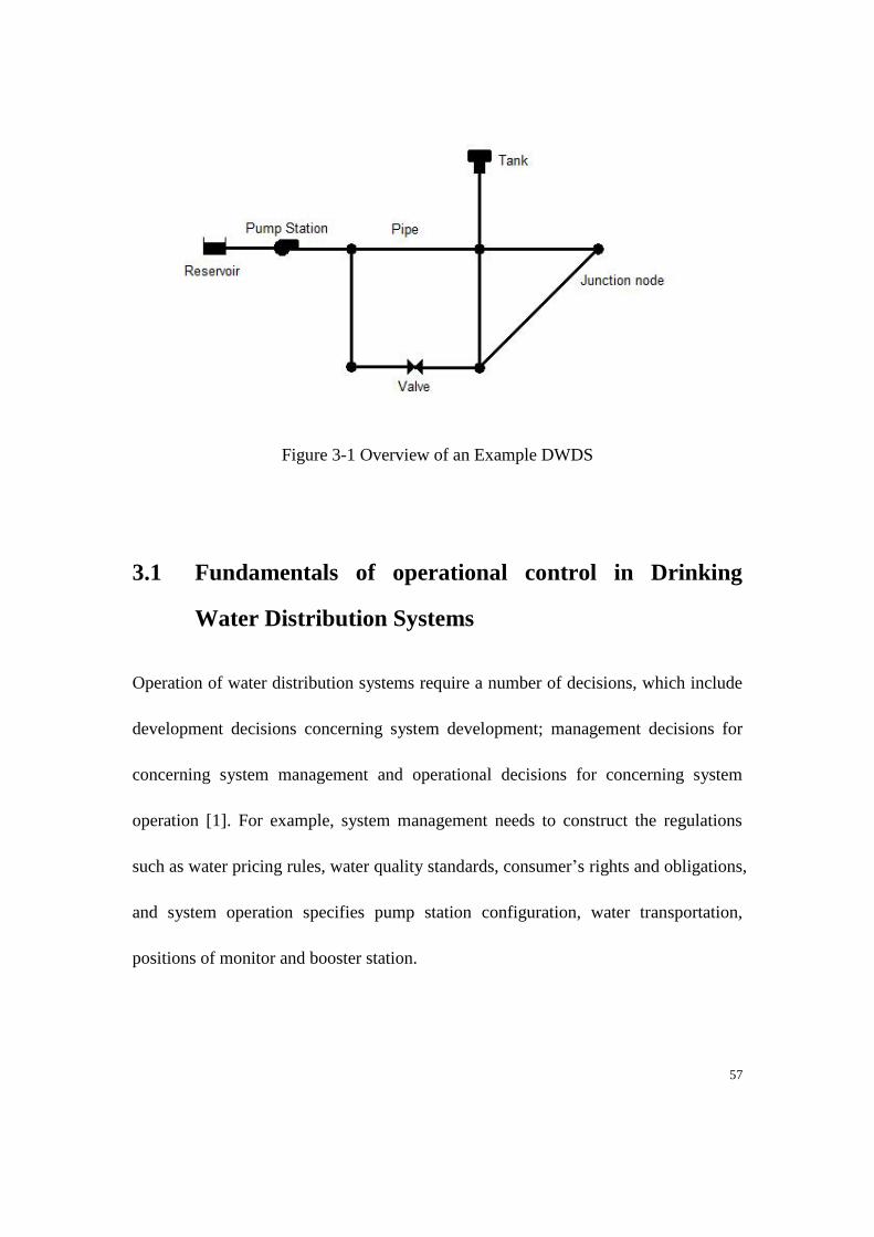
57
Figure 3-1 Overview of an Example DWDS
3.1 Fundamentals of operational control in Drinking
Water Distribution Systems
Operation of water distribution systems require a number of decisions, which include
development decisions concerning system development; management decisions for
concerning system management and operational decisions for concerning system
operation [1]. For example, system management needs to construct the regulations
such as water pricing rules, water quality standards, consumer’s rights and obligations,
and system operation specifies pump station configuration, water transportation,
positions of monitor and booster station.
58
Operational decisions are different from two other types of decision because they
change more frequently. Demand changes in the network or a security problem in the
system require a new operational decision to be made.
3.1.1 Objectives of Operational Control
The specific objectives of operational control in DWDS vary depending upon the
category of the water system. However, one of the common objectives is to satisfy the
physical constraints. For example, in terms of physical components in DWDS, there
are limitations on a retention reservoir which can be described as the maximum and
the minimum levels of the reservoir. In the viewpoint of water quality control,
maintaining the free disinfectant concentration (normally chlorine concentration) at a
prescribed value or range can also be formulated as a set of equalities or inequalities
constraints.
In this thesis, satisfying the objective of quality control not only considers the
constraints on disinfectant, but also considers the minimisation of DBPs concentration
in the specified network because DBPs are dangerous to people’s health.
Minimisation of operational cost is another control objective in the operational control
of DWDS [1]. Electricity costs due to pumping constitute the major operational cost
59
in DWDS. Moreover, the most important objective is to meet water demand generated
by every consumer in the DWDS.
Therefore, the overall objective of operational control in DWDS can be summarised
as: meeting water demand, satisfying the system constraints and minimising the
operating cost.
3.1.2 Handling Uncertainties
It is significant to note that any operational decision making process is uncertain [1].
The time horizon in the operational control of DWDS is great when compared to other
systems. Water demand is unknown at each hydraulic time step, values of parameters
in pipes is unknown (for example, roughness coefficient), leakage is unknown
regarding to time and position. Any of uncertainties mentioned above may require a
redesign for obtaining a desired operational performance under such uncertainty.
A fundamental tool used by a system operator when making operational decisions is a
predictive model of the specified system [1]. Predicting the uncertainty in systems
over the considered time periods is a typical approach to handling uncertainty. The
operational control problem becomes deterministic when the prediction of uncertainty
is produced. There are a number of prediction methods using different descriptions of
uncertainty which can be found in [1].
60
3.1.3 Basic Control Mechanisms
Two principle control mechanisms are utilised in the operational control of DWDS:
control rules and repetitive control, respectively [1].
The control rule embeds available measurements into a control signal or decision, and
the rule can be set up in the form of a table, formula, sets of written instruction, or
even a computer program [1].
The repetitive control is based on the internal model principle. And it emphasise to
reject or track arbitrary periodic signals during a fixed period [154]. The introduction
of the repetitive control theory and its application to operational control of water
systems can be found in [155].
3.2 Characteristics of Hydraulic Components and
Physical Laws in Drinking Water Distribution
Systems
The characteristics of water quality on transportation and mixing are mainly
determined by the water flows, flow velocities and detention times from reservoirs.
The hydraulic operation has a significant impact on the water quality modelling
however the effect brought by chlorine injections can be ignored under certain
61
accuracy. Modelling, simulation and operational control of water distribution systems
are presented in [1].
However, the characteristics of hydraulic components and their related physical laws
in DWDS are described here for better understanding the establishment of the water
quality model and uncertain sources in water quality control.
The following assumptions are made for the following models which are also applied
in the operational control of DWDS [2]:
1. The inertia effect of the water in the pipe is neglected;
2. Water is treated as incompressible fluid;
3. Constant temperature and air pressure within the DWDS;
4. Constant density and viscosity. Changes caused by injection of chlorine are
neglected;
5. Instantaneous dynamics of the water network components are neglected, e.g.
pump and valve on/off, and water pressure propagation dynamics in long
pipes.
The simplified instantaneous hydraulics will result in the above assumptions, however,
the control problems in DWDS are investigated in a time-scale from several minutes
to hours. Therefore, the inaccuracies caused by the above assumptions can be
considered as small and can be ignored while designing the controller [2].
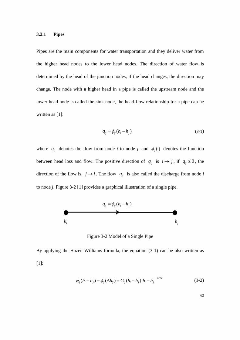
62
3.2.1 Pipes
Pipes are the main components for water transportation and they deliver water from
the higher head nodes to the lower head nodes. The direction of water flow is
determined by the head of the junction nodes, if the head changes, the direction may
change. The node with a higher head in a pipe is called the upstream node and the
lower head node is called the sink node, the head-flow relationship for a pipe can be
written as [1]:
( )ij ij i jq h h (3-1)
where ijq denotes the flow from node i to node j, and ( )ij denotes the function
between head loss and flow. The positive direction of ijq is i j , if 0ijq , the
direction of the flow is j i . The flow ijq is also called the discharge from node i
to node j. Figure 3-2 [1] provides a graphical illustration of a single pipe.
( )ij ij i jq h h
ih jh
Figure 3-2 Model of a Single Pipe
By applying the Hazen-Williams formula, the equation (3-1) can be also written as
[1]:
0.46
( ) ( ) ( )ij i j ij ij ij i j i jh h h G h h h h
(3-2)
63
where hij defines the head drop from the upstream node to the sink node in a pipe,
and the coefficient ijG presents the pipe conductivity. The Hazen-Williams equation,
the most frequently used method in modelling DWDS, is selected because it is simple
to calculate with acceptable accuracy which can meet the requirements of operational
control in DWDS.
The above equation can be solved by introducing the head drop across the pipe [2]:
1
( )ij i j ij ij ij ij ijh h h g q R q q
(3-3)
where ijR is the pipe resistance and α denotes the flow exponent caused by the
friction losses during the transportation. By applying the Hazen-Williams equation,
the equation (3-3) can be written as [1]:
0.852
10 1.852 4.87
( )
(1.21216 10 ) / ( )
ij i j ij ij ij ij ij
ij ij ij ij
h h h g q R q q
R L C D
(3-4)
where ijL , ijD and ijC denote the pipe length, diameter and Hazen-Williams
roughness coefficient, respectively. The value of the Hazen-Williams coefficient is
mainly determined by the material of the pipe, and it can be changed according to the
age of pipe, the manufacturer, workmanship and other factors [2]. If the pipe length
and diameter are in m and mm, and the heads are in m, then the resulting flow in
equation (3-1) are in litre/sec [1].
64
3.2.2 Valves
There exist several different kinds of valves used in DWDS for performing different
functions [156]:
Pressure Reducing Valves: Reduce water pressure
Pressure Sustaining Valves: Maintain the pressure at a specified value
Pressure Breaker Valves: Create required head loss across the valve
Check Valves: Control the flow direction in one way only
Flow Control Valves: Maintain the flow rate at a specified value
Pressure modulating valves, variable control valves, head control valves and
non-return control valves are normally used in DWDS. In this section, the variable
control valves are described as a modelling example, and one variable control valve is
illustrated in Figure 3-3 . The variable control valves can be modelled as a pipe with
controlled conductivity and are described as [1]:
0.46
( )ij ij ij i j i jq V G h h h h
(3-5)
where ijV is the valve control factor. The valve is closed if 0ijV , and fully opened
if 1ijV .
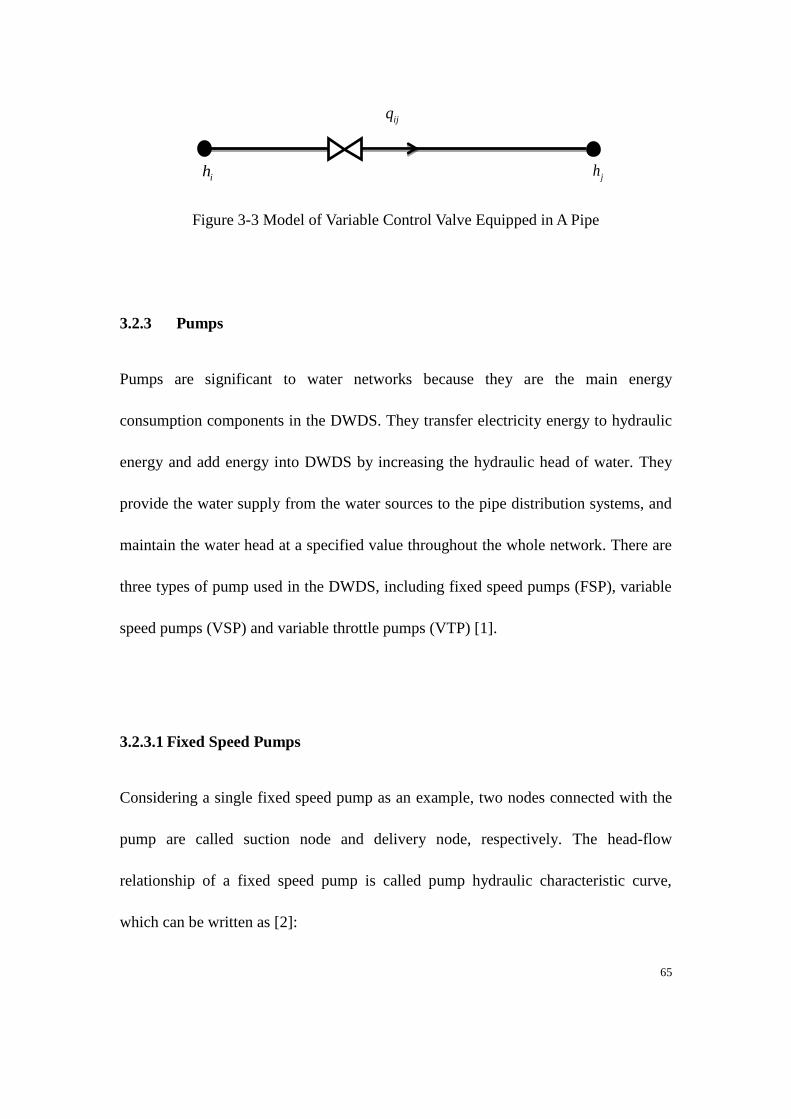
65
ijq
ih jh
Figure 3-3 Model of Variable Control Valve Equipped in A Pipe
3.2.3 Pumps
Pumps are significant to water networks because they are the main energy
consumption components in the DWDS. They transfer electricity energy to hydraulic
energy and add energy into DWDS by increasing the hydraulic head of water. They
provide the water supply from the water sources to the pipe distribution systems, and
maintain the water head at a specified value throughout the whole network. There are
three types of pump used in the DWDS, including fixed speed pumps (FSP), variable
speed pumps (VSP) and variable throttle pumps (VTP) [1].
3.2.3.1 Fixed Speed Pumps
Considering a single fixed speed pump as an example, two nodes connected with the
pump are called suction node and delivery node, respectively. The head-flow
relationship of a fixed speed pump is called pump hydraulic characteristic curve,
which can be written as [2]:
66
( )fs
ds sdh g q (3-6)
where ds d sh h h with
d sh h , sh and
dh are called suction head and delivery
head, respectively.sdq denotes the flow from the suction node to delivery node. The
superscript fs in ( )fs
sdg q presents ‘fixed speed’. Note that the pumping is always
from the ‘lower head’ to the ‘higher head’ and this is why pumps are the active
network elements and energy consumption components [1].
Equation (3-6) is a nonlinear function, and can be approximated by a quadratic
function [157, 158]:
2
,( )fs
sd sd sd sd sd so sdg q A q B q h (3-7)
where sdA is the resistance coefficient with 0sdA , and
sdB is a coefficient
normally taken as a value less than zero for guarantying a stable operating flow point
with headloss. ,so sdh is called the shut-off head [2].
Furthermore, pumps installed in the pump station can be operated in series or in
parallel. If the pumps are operating in series, the connected pumps have the same flow
but the total increasing head from the original node to the destination node is the sum
of increased heads generated by each pump. If the pumps are operating in parallel, the
increased heads generated by each switched on pump are the same but the flow from
original node to destination node is the sum of flows across each switched on pump.
67
For a group of U fixed speed pumps operated in parallel with u pumps switched on,
the hydraulic characteristic curves are the same and can be written as [1]:
( , )fs
ds sdh g q u (3-8)
2
,( ) ( ) , 0( , )
0 , 0
sd sdsd sd so sdfs
sd
q qA B h if u
u ug q u
if u
(3-9)
where [0, ]u U denotes the number of fixed speed pumps switched on.
3.2.3.2 Variable Speed Pumps
The pump speed of VSP can be continuously controlled over a certain speed range.
Considering a single VSP as an example, the hydraulic characteristic curve can be
written as:
( , )vs
ds sd sd sdh g q s (3-10)
where sds presents the pump speed and is defined as [1]:
sd
operating speeds
nominal speed (3-11)
The nonlinear equation (3-10) can also be approximated by a quadratic function and
written as [157, 158]:
68
2 2
,( , )vs
sd sd sd sd sd sd sd so sd sdg q s A q B q s h s (3-12)
For a group of U variable speed pumps running in parallel with u pumps switched on,
the hydraulic characteristic curves of these pumps are the same and can be written as
[1]:
( , , )vs
ds sd sd sdh g q s u (3-13)
2 2
,( ) ( ) , 0, 0( , , )
0
sd sdsd sd sd so sd sd sd sdvs
sd sd
q qA B s h s if s and u
u ug q s u
otherwise
(3-14)
where [0, ]u U denotes the number of variable speed pumps switched on.
3.2.3.3 Variable Throttle Pumps
Based on the flow described in equation (3-1), the inverse function of equation (3-13)
can be defined as [1]:
( , , )sd sd sdq h s u (3-15)
Then, the hydraulic characteristic curves for a group of U variable throttle pumps in
parallel with u pumps switched on can be written as [1]:
( , ) ( , )fs t
ds sd sdh g q u h q v (3-16)
69
where [0, ]u U , variable v is control factor for the throttle conductivity.
The above equation describes the final head increase from the delivery node to
suction node. There are two parts to the right side of equation (3-16), the first part
presents the total increased head from the group of fixed speed pumps, and the second
part presents the head drop across the throttle and can be modelled as a variable
control valve.
3.2.3.4 Pump Station
In general, pumps installed in the network are considered as the form of pump stations.
The structure of a pump station consisting of all types of pumps in parallel is
illustrated in Figure 3-4 [1]. The figure illustrates the configuration of the thi pump
station in the total of I pump stations in a network, where f
iM fixed speed pumps,
s
iM variable speed pumps and t
iM variable throttle pumps are contained within the
thi pump station. Notations iq or piq present the overall pump flow in the pump
station. sih and
dih are the suction head and delivery head, respectively.
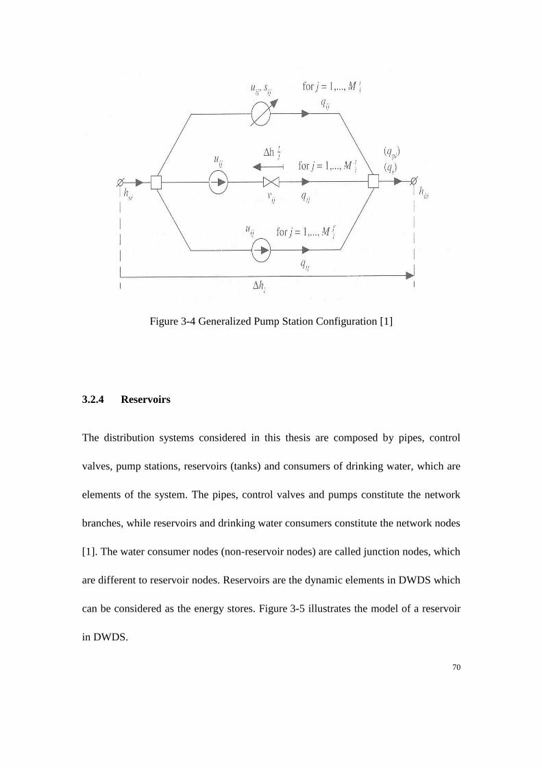
70
Figure 3-4 Generalized Pump Station Configuration [1]
3.2.4 Reservoirs
The distribution systems considered in this thesis are composed by pipes, control
valves, pump stations, reservoirs (tanks) and consumers of drinking water, which are
elements of the system. The pipes, control valves and pumps constitute the network
branches, while reservoirs and drinking water consumers constitute the network nodes
[1]. The water consumer nodes (non-reservoir nodes) are called junction nodes, which
are different to reservoir nodes. Reservoirs are the dynamic elements in DWDS which
can be considered as the energy stores. Figure 3-5 illustrates the model of a reservoir
in DWDS.
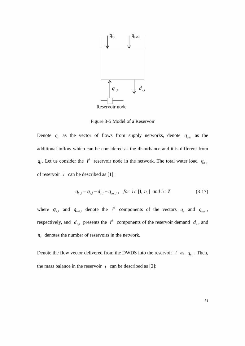
71
,s iq ,out iq
,r iq ,r id
Reservoir node
Figure 3-5 Model of a Reservoir
Denote sq as the vector of flows from supply networks, denote
outq as the
additional inflow which can be considered as the disturbance and it is different from
sq . Let us consider the thi reservoir node in the network. The total water load ,lr iq
of reservoir i can be described as [1]:
, , , , , [1, ]lr i s i r i out i rq q d q for i n and i Z (3-17)
where ,s iq and ,out iq denote the thi components of the vectors sq and
outq ,
respectively, and ,r id presents the thi components of the reservoir demand rd , and
rn denotes the number of reservoirs in the network.
Denote the flow vector delivered from the DWDS into the reservoir i as ,r iq . Then,
the mass balance in the reservoir i can be described as [2]:
72
, ,
( )[ ( ) ], [1, ]i
r i lr i r
d w tq t q for i n and i Z
dt (3-18)
where is the water density, ( )iw t denotes the mass of water stored in the
reservoir i at time instant t . Then, substituting the water head and cross-sectional
area of the reservoir into equation (3-18) yields [2]:
, ,
( ) 1[ ( ) ], [1, ]
( ( ))
ir i lr i r
i i
d x tq t q for i n and i Z
dt S x t (3-19)
, ( ) ( ) , [1, ]r i i i rh t x t E for i n and i Z (3-20)
Substituting equation (3-20) into equation (3-19) yields:
,
, ,
,
( ) 1[ ( ) ], [1, ]
( ( ))
r i
r i lr i r
i r i
d h tq t q for i n and i Z
dt S h t (3-21)
where ( )ix t , ( ( ))i iS x t and , ( )r ih t presents level of reservoir i , the cross-sectional
area at this level and reservoir head, respectively. iE is the reservoir elevation.
3.2.5 Physical Laws
3.2.5.1 Flow Continuity Law
For every junction node (non-reservoir node) j in the network, the following holds
(see Figure 3-6):
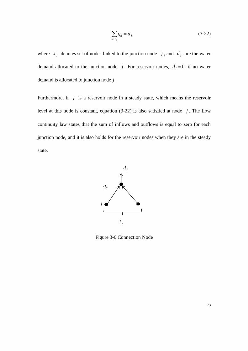
73
j
ij j
i J
q d
(3-22)
where jJ denotes set of nodes linked to the junction node j , and jd are the water
demand allocated to the junction node j . For reservoir nodes, 0jd if no water
demand is allocated to junction node j .
Furthermore, if j is a reservoir node in a steady state, which means the reservoir
level at this node is constant, equation (3-22) is also satisfied at node j . The flow
continuity law states that the sum of inflows and outflows is equal to zero for each
junction node, and it is also holds for the reservoir nodes when they are in the steady
state.
jd
ijq
i
jJ
Figure 3-6 Connection Node
74
3.2.5.2 Energy Conservation Law
The energy conservation law is usually expressed in terms of the head change
(increases or drops) along a loop or an energy path. The following holds:
ij rh E (3-23)
where ij i jh h h is the head change (increases or drops) across an arc (link) in thr
network path, and rE denote the energy difference between the starting node and
final node on this path.
If the starting node is the same as the final node, which means the path existed as a
loop in a network, the following holds:
0ijh (3-24)
The energy conservation law is applicable to all network paths that can produce the
number of equations of the type described in equation (3-23) [1].
3.3 Path Analysis Algorithm
Only the input-output (IO) model is considered in this thesis, therefore, it is important
to consider the transportation path from the injection node (input) to the monitored
node (output) and the time delay associated with the path. In this section, the
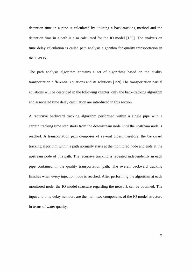
75
detention time in a pipe is calculated by utilising a back-tracking method and the
detention time in a path is also calculated for the IO model [159]. The analysis on
time delay calculation is called path analysis algorithm for quality transportation in
the DWDS.
The path analysis algorithm contains a set of algorithms based on the quality
transportation differential equations and its solutions [159] The transportation partial
equations will be described in the following chapter, only the back-tracking algorithm
and associated time delay calculation are introduced in this section.
A recursive backward tracking algorithm performed within a single pipe with a
certain tracking time step starts from the downstream node until the upstream node is
reached. A transportation path composes of several pipes; therefore, the backward
tracking algorithm within a path normally starts at the monitored node and ends at the
upstream node of this path. The recursive tracking is repeated independently in each
pipe contained in the quality transportation path. The overall backward tracking
finishes when every injection node is reached. After performing the algorithm at each
monitored node, the IO model structure regarding the network can be obtained. The
input and time delay numbers are the main two components of the IO model structure
in terms of water quality.
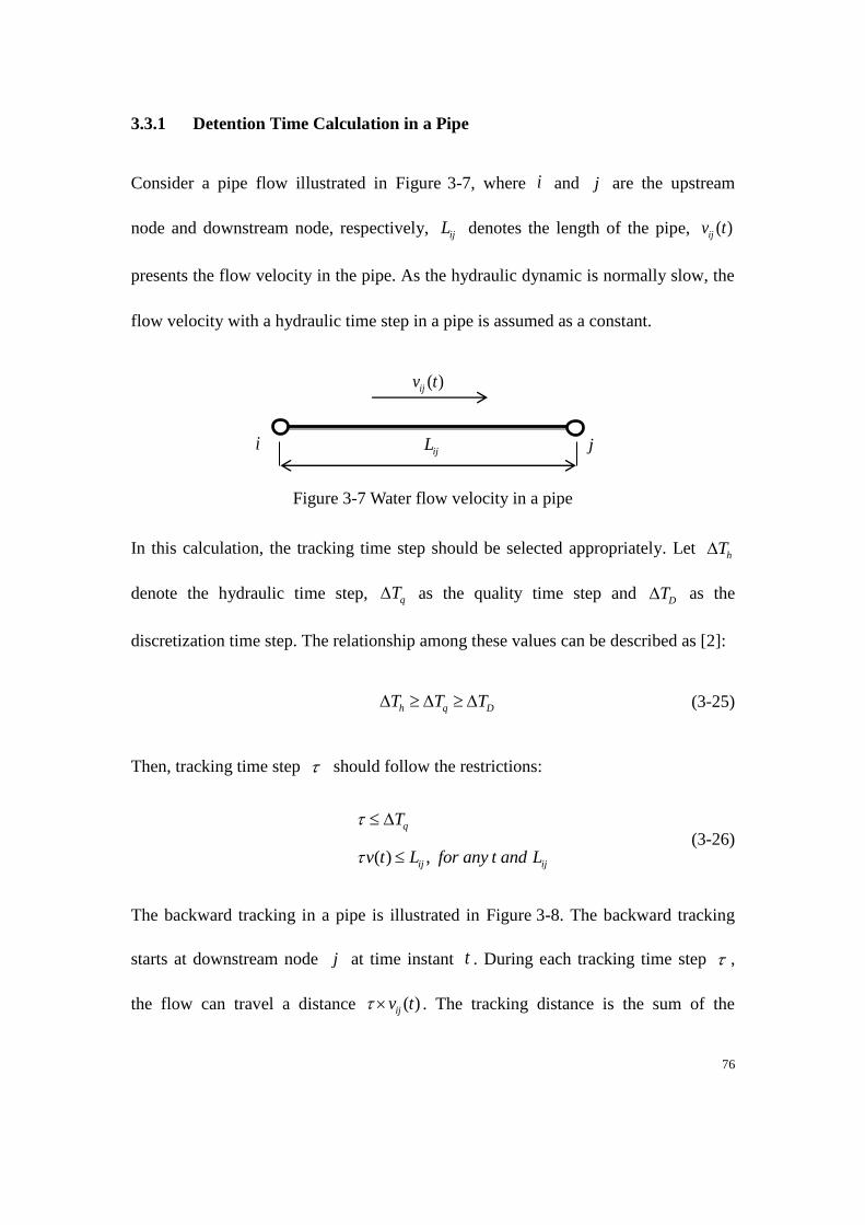
76
3.3.1 Detention Time Calculation in a Pipe
Consider a pipe flow illustrated in Figure 3-7, where i and j are the upstream
node and downstream node, respectively, ijL denotes the length of the pipe, ( )ijv t
presents the flow velocity in the pipe. As the hydraulic dynamic is normally slow, the
flow velocity with a hydraulic time step in a pipe is assumed as a constant.
( )ijv t
i ijL j
Figure 3-7 Water flow velocity in a pipe
In this calculation, the tracking time step should be selected appropriately. Let hT
denote the hydraulic time step, qT as the quality time step and DT as the
discretization time step. The relationship among these values can be described as [2]:
h q DT T T (3-25)
Then, tracking time step should follow the restrictions:
( ) ,
q
ij ij
T
v t L for any t and L
(3-26)
The backward tracking in a pipe is illustrated in Figure 3-8. The backward tracking
starts at downstream node j at time instant t . During each tracking time step ,
the flow can travel a distance ( )ijv t . The tracking distance is the sum of the
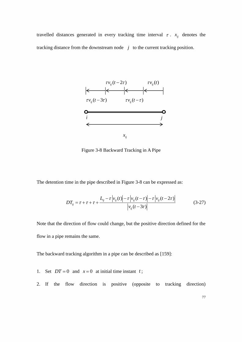
77
travelled distances generated in every tracking time interval . ijx denotes the
tracking distance from the downstream node j to the current tracking position.
( 2 )ijv t ( )ijv t
( 3 )ijv t ( )ijv t
i j
ijx
Figure 3-8 Backward Tracking in A Pipe
The detention time in the pipe described in Figure 3-8 can be expressed as:
( ) ( ) ( 2 )
( 3 )
ij ij ij ij
ij
ij
L v t v t v tDT
v t
(3-27)
Note that the direction of flow could change, but the positive direction defined for the
flow in a pipe remains the same.
The backward tracking algorithm in a pipe can be described as [159]:
1. Set 0DT and 0x at initial time instant t ;
2. If the flow direction is positive (opposite to tracking direction)
78
( )x x v t DT ;
else ( )x x v t DT ;
3. If x L , set DT DT , and go to step 2;
else ( )
( )
L x v t DTDT DT
v t DT
, set the current node to i , end.
3.3.2 Detention Time Calculation in a Path
An illustration of transportation paths for delivering water quality from source node
(injection node) A to monitored node G in a DWDS is shown in Figure 3-9 [159].
As shown in Figure 3-9, A, B, C, D, E, F and G denote junction nodes in paths. There
are 4 different paths transporting water quality from the injection node A to monitored
node G, including path A-B-C-E-G, path A-D-E-G, path A-F-G and path A-C-E-G,
respectively. Several single pipes are presented by a, b, c, d, e and f.
Figure 3-9 Illustration of Transportation Paths in a DWDS
Take detention time of path A-C-E-G as an example for calculation [2]:
F
A C G
D
E
B
a
b
c
d
e
f
Input Output
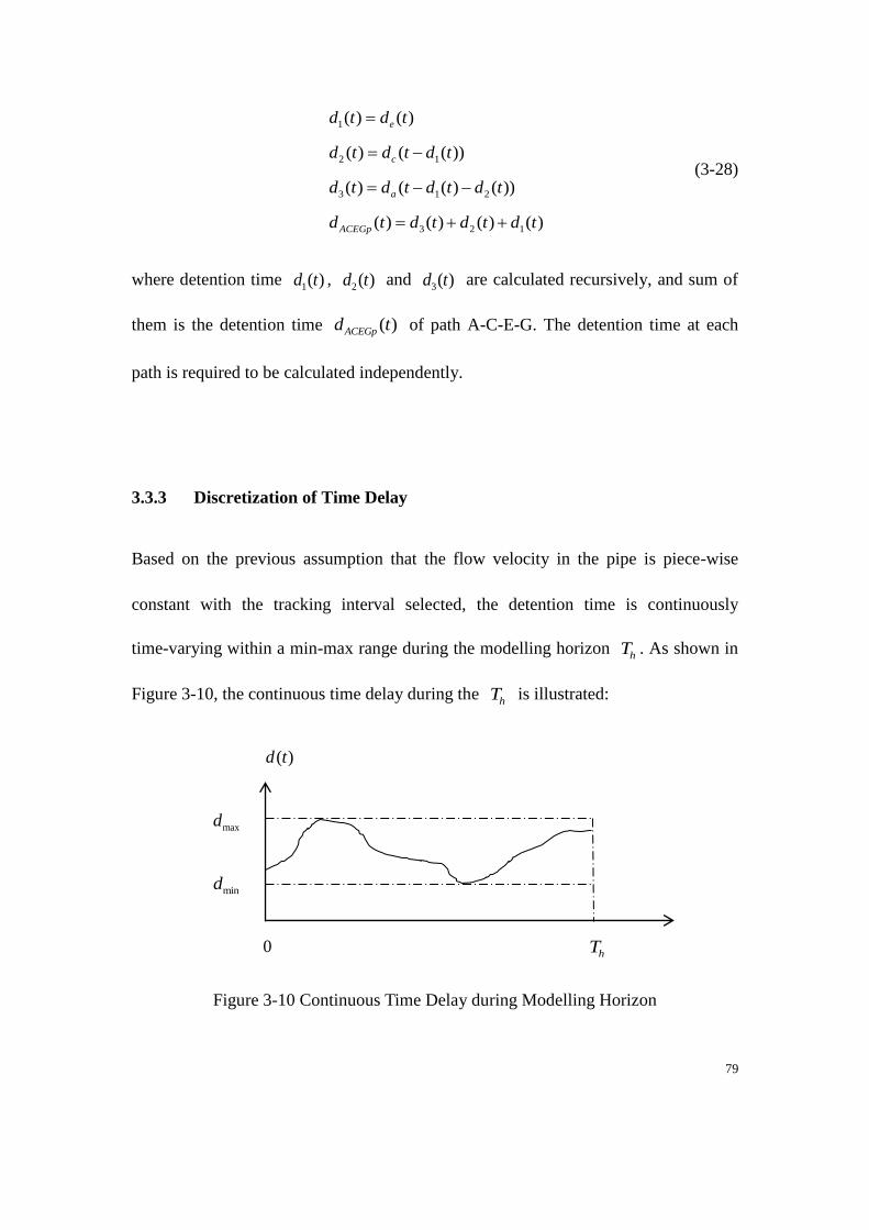
79
1
2 1
3 1 2
3 2 1
( ) ( )
( ) ( ( ))
( ) ( ( ) ( ))
( ) ( ) ( ) ( )
e
c
a
ACEGp
d t d t
d t d t d t
d t d t d t d t
d t d t d t d t
(3-28)
where detention time 1( )d t ,
2( )d t and 3( )d t are calculated recursively, and sum of
them is the detention time ( )ACEGpd t of path A-C-E-G. The detention time at each
path is required to be calculated independently.
3.3.3 Discretization of Time Delay
Based on the previous assumption that the flow velocity in the pipe is piece-wise
constant with the tracking interval selected, the detention time is continuously
time-varying within a min-max range during the modelling horizon hT . As shown in
Figure 3-10, the continuous time delay during the hT is illustrated:
( )d t
maxd
mind
0 hT
Figure 3-10 Continuous Time Delay during Modelling Horizon
80
The continuous variations in time delay are not applicable for modelling the water
quality dynamic model numerically within the selected time interval or simulation
time step. Therefore, the delay range is required to be discretized into a series of delay
numbers and the continuous detention time can be approximated by these delay
numbers [94, 160]. Delay numbers can be defined as:
min min max max
minmin
maxmax
, 1,..., 1,
( )
( )
ij
D
D
I n n n n
dn round
T
dn round
T
(3-29)
where DT denotes the discretization time step, function (.)round aims to find the
closest real integer number, ijI presents the delay number in pipe ijp over the time
period [0, ]hT . Normally, a structure error caused by discretization should be
considered, which is to be discussed later in the following chapters.
3.4 Summary
This chapter explored the DWDS physical modelling and its operational control, and
also explored the path analysis algorithm for detention time calculation.
The fundamentals of operational control in DWDS have been introduced under three
main aspects, i.e. objectives, uncertainty handling and basic control mechanisms,
81
respectively. The background of operational control of DWDS leads to a greater
understanding of water quality control in DWDS.
The physical components installed in DWDS have also been described and illustrated,
and each of them plays an irreplaceable role in water quality control. The physical
laws, including flow continuity law and energy conservation law, were illustrated and
described. Note that, hydraulic information is significant for the control of water
quality in DWDS because it contains the input information for water quality control.
The path analysis algorithm has been introduced in this chapter, and the calculation of
detention time in a pipe and in a path is formulated and will be applied in the
following application to the deriving water quality IO model.
82
CHAPTER 4 APPLICATION OF NONLINEAR
MODEL PREDICTIVE CONTROL ON WATER
QUALITY IN DWDS WITH DBPS INVOLVED
This chapter develops a nonlinear model predictive controller to implement optimising
control on water quality in DWDS. The water quality model utilised in the controller
is based on the advanced nonlinear water quality dynamics model, which jointly
considers the disinfection and the augmented control objective-DBPs. Based on the
newly developed two time-scale architecture of the integrated control of quantity and
quality in DWDS, the interest on analysing the impact brought by flow trajectories
optimised by the upper level optimisation controller is increased. The applied
nonlinear model predictive control (NMPC) is to operate in a fast time-scale as the
same as the lower level quality controller within this architecture. The NMPC
algorithm is to be applied to a comprehensive simulation study based on an example
network with nonlinear water quality dynamics. The performance of the controller is
validated by the related simulation results.
In this chapter, the hierarchical two-level structure for optimising integrated quantity
and quality control will be introduced. The information from the upper level is
83
considered as the priori known. Only the lower level controller for controlling water
quality with DBPs is considered in this chapter. In addition, the MPC methodology is
described in this chapter.
4.1 Introduction to the Hierarchical Two-Level Structure
in DWDS
An increasing shortage of natural water resources around the world has been observed,
due to climate change, a rising population and environment pollution[35, 36].
Therefore, meeting the demand for drinking water of a required quality requires
advanced control technology to operate DWDS which are typically large scale complex
network systems [1].
As described in Chapter 3, quantity and quality are the two primary aspects from the
control viewpoint of DWDS. The quantity control aims to handle the flow of pipes and
pressure of the junction nodes in water system by producing the optimised pump and
valve control schedules. The main objectives of quantity control are: 1) meet the real
water demand at the user nodes, and 2) minimise electrical energy cost due to pumping
[1, 12].
84
As described in Chapter 2, one of quality control objectives aims to maintain the free
disinfectant concentration at the monitored nodes. The maintained level of free
disinfectant concentration must satisfy the user-defined limits prescribed in such a way
that the bacterial re-growth over a whole DWDS is halted. However, the free
disinfectant reacts with the organic matters over the DWDS producing so called
disinfectant by-products (DBPs), which are dangerous to health [14].
Therefore, the DBP concentrations over the DWDS ought to be kept as low as possible
and this is another objective of the quality control. Chlorine is considered as the
disinfectant because of its low price and effectiveness. Therefore, the free chlorine
concentration is often used for assessment of the water quality state [93]. In summary,
the quality control aims to maintain free chlorine concentrations at the monitored nodes
within the described lower-upper limits and minimising the DBP concentrations at
these nodes.
The chlorine residuals are controlled by the treatment plant to ensure the water has the
satisfied residual values when enter into the DWDS. However, with the water
travelling throughout the whole network, the disinfectant reacts with bacteria and
organic matters and it leads to its major decay and generation of DBPs so that the
security of water may not be guaranteed, especially at several remote consumption
nodes.
85
As a result, it is necessary to inject chlorine by employing booster stations located at
selected intermediate junction nodes in DWDS. The chlorine injections are the only
quality control inputs considered in this thesis because the hydraulic information is
assumed as a priori known, while the booster stations are the corresponding quality
actuators. The optimised allocation of the booster station problem was presented in [71,
74].
The quality concentrations can change rapidly because of the decay, mixing of water
flows, even by consumption of physical materials during water transportation. The
detention time described in chapter 3 from the source to the monitored nodes
significantly depends on the hydraulic operation of the network. The quantity control
has important effects on the quality control. However, the quality control inputs
(injection) have no impact on the flows which are the hydraulic controlled outputs
because the injected disinfectant mass can be negligible when compared to the mass
of water. Nevertheless, the quality controlled outputs depend on the flows. Therefore,
the quality and quantity interaction exists although it is only one way interaction from
quantity to quality, and both quality and quantity are required to be controlled in an
integrated manner.
In the operational control of DWDS, the quantity control problem is normally
formulated based on the demand prediction over a certain control horizon, which is
typically 24 hours. In general, the prediction step used in DWDS is 1 hour or 2 hours,
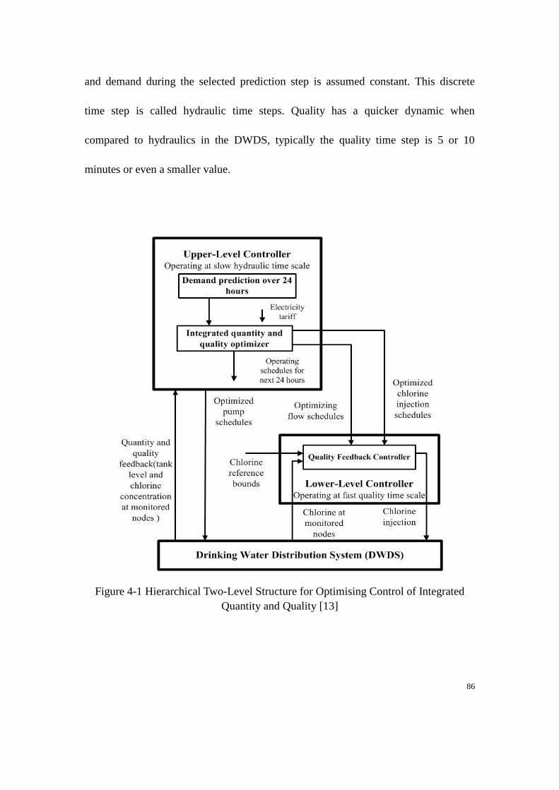
86
and demand during the selected prediction step is assumed constant. This discrete
time step is called hydraulic time steps. Quality has a quicker dynamic when
compared to hydraulics in the DWDS, typically the quality time step is 5 or 10
minutes or even a smaller value.
Figure 4-1 Hierarchical Two-Level Structure for Optimising Control of Integrated
Quantity and Quality [13]
87
As a result of the multi time-scales in the dynamics of hydraulic and quality, which is
slow and fast respectively, a dimension complexity of the integrated MPC optimisation
task is large. This makes direct application of NMPC algorithm to integrated control of
water quality and quantity even for a small size DWDS impossible [16]. Therefore, a
two time-scale hierarchical control structure was proposed in [17] and [18] for jointly
considering the two different time scale problems and the structure is illustrated in
Figure 4-1.
The optimisation controller at Upper Control Level (UCL) operates in a slow hydraulic
time scale based on the accurate hydraulic model and simplified quality model with one
hour time step applied to both models. The models are used to predict the quantity and
quality controlled outputs over the quantity prediction horizon of 24 hours.
Water quantity and quality are estimated or measured at beginning of a control period,
and then sent to an integrated optimiser. Moreover, the water demand prediction is
provided for the optimiser as well. Following the one way interaction between the
quantity and quality, the hydraulic optimisation control resulting from solving the MPC
optimisation task are truly optimal.
The quality dynamic model in the optimisation problem has the same time step as the
quantity dynamic model. Although the problem dimension is decreased immensely, the
error in modelling quality is extremely increased. Therefore, the quality controls need
88
to be improved and this is done at the Lower Correction Level (LCL) by employing the
fast quality feedback controller operating at the fast quality time scale. The hydraulic
controlled outputs, which are flows, needed at the LCL by the fast quality controller are
taken as determined at the UCL. The quality residuals are sampled at the rate required
by the decay dynamics of the disinfectant [12, 16]and the growth dynamics of the DBPs
[7, 161].
In order to achieve the operational objectives of DWDS described in chapter 3 in a
robustly feasible and cost effective way, information about the DWDS states, including
quantity and quality, is required on-line. Monitoring of the water quantity has been well
developed in previous research, while the quality monitoring is also presented in [7, 92].
Optimised placement of hard chlorine sensors achieving the required balance between
the estimation accuracy and sensor maintenance and capital cost is presented in [162].
Presently, only the bacterium objective is considered for the quality control under the
MPC control methodology [2, 39]. In this thesis both the chlorine and DBPs are jointly
considered and the MPC is applied to synthesize the Lower Level Controller (LLC) at
LCL of the structure in Figure 4-1.
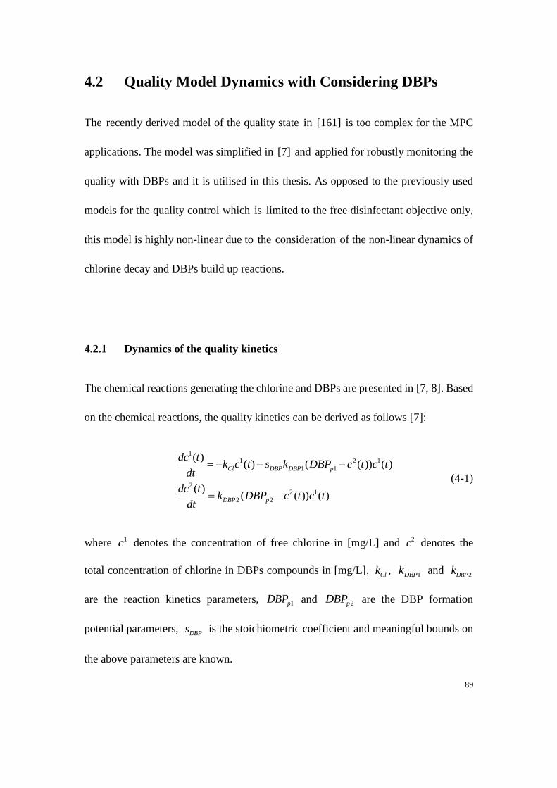
89
4.2 Quality Model Dynamics with Considering DBPs
The recently derived model of the quality state in [161] is too complex for the MPC
applications. The model was simplified in [7] and applied for robustly monitoring the
quality with DBPs and it is utilised in this thesis. As opposed to the previously used
models for the quality control which is limited to the free disinfectant objective only,
this model is highly non-linear due to the consideration of the non-linear dynamics of
chlorine decay and DBPs build up reactions.
4.2.1 Dynamics of the quality kinetics
The chemical reactions generating the chlorine and DBPs are presented in [7, 8]. Based
on the chemical reactions, the quality kinetics can be derived as follows [7]:
11 2 1
1 1
22 1
2 2
( )( ) ( ( )) ( )
( )( ( )) ( )
Cl DBP DBP p
DBP p
dc tk c t s k DBP c t c t
dt
dc tk DBP c t c t
dt
(4-1)
where 1c denotes the concentration of free chlorine in [mg/L] and 2c denotes the
total concentration of chlorine in DBPs compounds in [mg/L], Clk ,
1DBPk and 2DBPk
are the reaction kinetics parameters, 1pDBP and 2pDBP are the DBP formation
potential parameters, DBPs is the stoichiometric coefficient and meaningful bounds on
the above parameters are known.
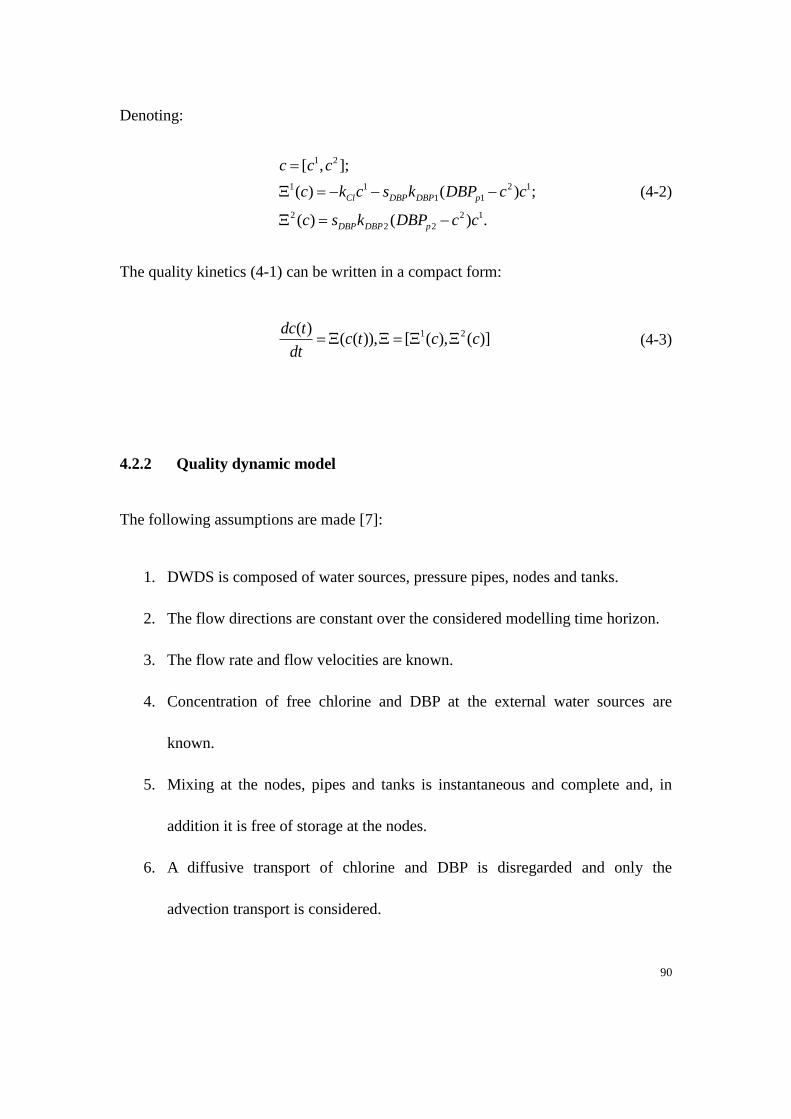
90
Denoting:
1 2
1 1 2 1
1 1
2 2 1
2 2
[ , ];
( ) ( ) ;
( ) ( ) .
Cl DBP DBP p
DBP DBP p
c c c
c k c s k DBP c c
c s k DBP c c
(4-2)
The quality kinetics (4-1) can be written in a compact form:
1 2( )( ( )), [ ( ), ( )]
dc tc t c c
dt (4-3)
4.2.2 Quality dynamic model
The following assumptions are made [7]:
1. DWDS is composed of water sources, pressure pipes, nodes and tanks.
2. The flow directions are constant over the considered modelling time horizon.
3. The flow rate and flow velocities are known.
4. Concentration of free chlorine and DBP at the external water sources are
known.
5. Mixing at the nodes, pipes and tanks is instantaneous and complete and, in
addition it is free of storage at the nodes.
6. A diffusive transport of chlorine and DBP is disregarded and only the
advection transport is considered.
91
The quality dynamic model considers the change of chlorine and DBPs concentrations
at junction nodes, tanks and along pipes. By applying (4-3) the quality advection
transport along a pipe p NP with length pL can be described as [7, 163]:
( , ) ( , )( , ) ( ( , ))
p p
p p
c l t c l tv l t c l t
t l
(4-4)
Equation (4-4) is constrained by the initial and boundary condition ( ,0), [0, ]p pc l l L
and (0, ),pc t p NP respectively, where ( , )pc l t denotes the quality state at time t at
distance l from the pipe flow entry point 0l , ( )pv t denotes the pipe flow velocity
and NP is the number of pipes. Since the water is assumed incompressible and the pipes
are of the pressure type, then ( , ) ( )p pv l t v t for [0, ],pl L p NP .
After partitioning each pipe p into the PNS segments with length pl , and then
defining ( , ) ( , )p p pc m t c m l t , where 1,..., pm NS , equation (4-4) can be
approximated in space as [7, 92]:
( , ) ( , ) ( 1, )( , ) ( ( , ))
p p p
p p
p
dc m t c m t c m tv l t c m t
dt l
(4-5)
where: ( 1, ) (0, )p pc m t c t for 1m .
The variables 1 2( 1, ) [ ( 1, ), ( 1, )], 1,...,p p p pc m t c m t c m t m NS , are composed of
the state variables of a quality model dynamics in pipe p and (4-5) are the state
equations.
92
Next, in considering the water quality mixing at the pipe junction node n NPJ at
time instant t, the following denotations are made: IIn, EIn presents the sets of pipes
delivering the water from the DWDS and external sources respectively, into the node n
at time instant t; 1
, ( )in nc t denotes the free chlorine dosing into the node n by flow paced
booster quality controlling devices [12].
The pipe junction nodes with the dosing are the quality control nodes (CNPJ). For
practical reasons a set of these nodes CNPJ is limited to only achieving controllability
of the quality [164]. The quality control inputs are 1
, (t)in nc , where
n CNPJ NPJ .The resulting quality output ( )nc t at the junction node n can be
expressed as [7]:
,
( ) ( , ) ( ) ( , )
( ) ( )( ) ( )
p p p p p p
p IIn p EIn
n in n
p p
p IIn p EIn
q t c L t q t c L t
c t c tq t q t
(4-6)
where 1
, ,( ) [ ( ),0]T
in n in nc t c t , ( )pq t is the pipe flow at time instant t.
Furthermore, consider the quality dynamics in the tank. As for the pipe junction nodes,
denoting ITH(t) as the set of pipes delivering water in the tank h NT at time instant t,
the quality model dynamics can be described as [7, 92]:
,
,
,
,
( )( ( , ) (t))(t)
( (t))(t)
p p p T h
p IThT h
T h
T h
q t c L t cdc
cdt V
(4-7)
93
where: , (t)T hc is the quality state in tank h and , (t)T hV is the tank water volume at time
instant t.
The quality monitored nodes with the prescribed concentration bounds are the quality
control outputs and (4-6) are the output equations in the quality state-space model.
It is now clear that the quality state-space model described above is a non-linear
time-varying dynamical system with the input and output constraints. As the free
chlorine and DBP concentrations can be measured on-line by hard sensors located only
at very limited number of elements of NPJ, the quality state must be estimated for
control purposes.
4.3 Optimising Model Predictive Controller for Water
Quality with Augmented DBPs Objective
Due to the nonlinear dynamics described in the quality model with DBPs involved, and
the multivariable constrained optimisation control problems, the MPC methodology is
selected as the core algorithm to implement the optimising quality control with
considering the augmented DBPs objective at DWDS. Both chlorine and DBPs are
considered as the control objectives in the nonlinear MPC controller. The details
regarding to design the nonlinear MPC controller are to be presented in the following
sections.
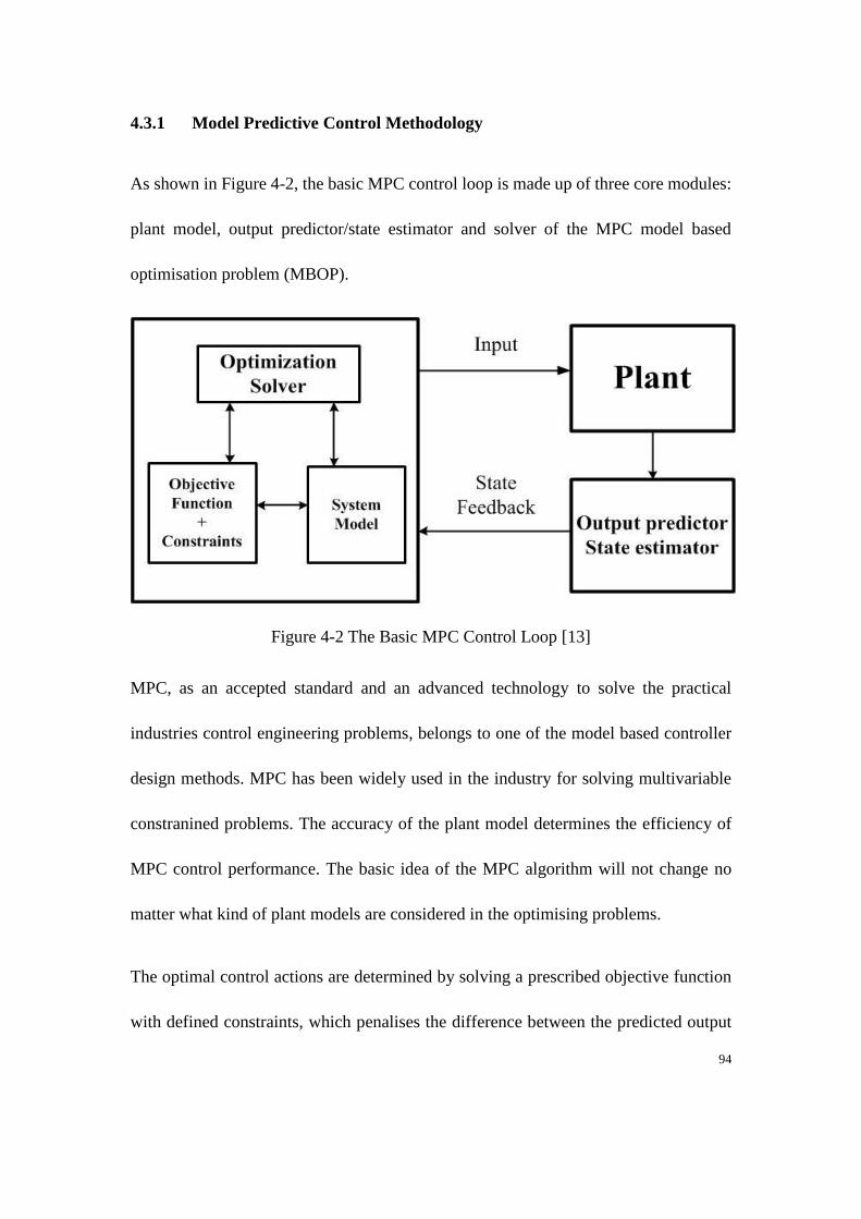
94
4.3.1 Model Predictive Control Methodology
As shown in Figure 4-2, the basic MPC control loop is made up of three core modules:
plant model, output predictor/state estimator and solver of the MPC model based
optimisation problem (MBOP).
Figure 4-2 The Basic MPC Control Loop [13]
MPC, as an accepted standard and an advanced technology to solve the practical
industries control engineering problems, belongs to one of the model based controller
design methods. MPC has been widely used in the industry for solving multivariable
constranined problems. The accuracy of the plant model determines the efficiency of
MPC control performance. The basic idea of the MPC algorithm will not change no
matter what kind of plant models are considered in the optimising problems.
The optimal control actions are determined by solving a prescribed objective function
with defined constraints, which penalises the difference between the predicted output
95
from the specified reference or limits. The control action at each MPC time step is
calculated on-line by solving a finite-horizon open-loop optimisation problem [165].
The current states of the plant are used as the initial states of the optimisation problem
for the next MPC time step. Only the first part of the optimised control sequence is
utilised as the control action applied into the real plant. At a MPC control time step,
the user-defined prediction horizon moves forward and the same procedure repeats till
the modelling horizon ends.
Denote kx as the states of the plant at time k , ku as the first part of the optimised
control action (input) applied to the plant, then the basic MPC algorithm can be
expressed as:
1. Measure or estimate kx at time k ;
2. Determine the prediction horizon and control horizon based on the
characteristics of target systems;
3. Obtaining ku by solving the user defined objective functions, and applying
ku to the plant;
4. Set 1k k , go to step 1 till the modelling horizon ends.
96
4.3.2 Formulation of MBOP
Denote ( )iu t and y ( )j t as the input and controlled output of the proposed control
system respectively. The ( )iu t is composed of the chlorine injections at the quality
control nodes CNPJ, and 1 2( ) [ ( ), ( )]jj jy t y t y t , j MNPJ denotes the free chlorine
and DBP concentrations, respectively, at the quality monitored nodes MNPJ. Based on
analysis of the control objectives described in section 1, the constraints in the MBOP
are formulated as:
min max
1min 1 1max
( ) ( ) ( );
( ) ( ) ( ).
i i i
j j j
u t u t u t
y t y t y t
(4-8)
where min ( )iu t ,
max ( )iu t , 1min ( )jy t and 1max ( )jy t are the upper and lower bounds on
inputs and outputs in CNPJ and MNPJ, respectively.
Moreover, maintaining the DBP concentrations as small as possible is vital. Hence, the
objective function is formulated as:
2( ) min ( ( ))P
j
t H j MNPJ
f t y t
(4-9)
where PH presents the defined prediction horizon in MBOP.
4.3.3 State Feedback
Given control sequence over the prediction horizon, the forced output is determined by
applying the state-space quality model. However, as the states are not measurable, they
97
must be estimated. The newly derived state estimator in [7] is applied to produce the
robust state estimates on-line. DWDS state variables like 1) the free chlorine and DBP
concentrations along pipes, 2) tank heads and 3) free chlorine and DBP concentrations
in tanks are required to measured or estimated. Denoting the state vector at time instant
t as [18]:
, ,( ) { ( ), ( ), ; ( , ), [0, ], }T h T h p pX t H t c t h NT c l t l L p NP (4-10)
where: , ( )T hH t presents as tank head of tank h at time instant t.
Then the MPC controller operates at kT as follows:
1. States of DWDS X(kT) is measured or estimated. While, the water demand and
DWDS quality boundary conditions are predicted.
2. The optimisation problem (4-9) in nonlinear MPC controller is solved.
3. Apply the first optimised control action into DWDS.
4. Set 1k k and return to step 1.
4.3.4 Solver of MBOP
The optimiser is designed as performing the search in the space of the control inputs.
This is supported by employing a fast and reliable simulator of the quality at DWDS.
Hence, the Genetic Algorithm (GA) is applied to solve the optimisation problem as
98
faster non-linear optimisation algorithms such as SQP are hardly applicable to the
chosen structure of the optimisation search (the gradients and second derivatives are
not analytically available). The initial quality states are provided by the state estimator.
GA begins with a random population of individuals and/or a designer-selected
population. The algorithms stop when one or more of pre-established criteria, such as
the number of generations or fitness tolerance, are met [165].
4.3.5 Model Simulator: EPANET AND EPANET-MSX
EPANET is a software package published by the National Risk Management Research
Laboratory of United State Environment Protection Agency in 2000. Normally, it is
used in water system simulation and hydraulic behaviour design with pressurized pipe
networks. Constructing the distribution of water systems, calibrating and tuning the
coefficients of water systems are the main functions of EPANET. Moreover, EPANET
can generate the EPANET input file which stores the simulation data for the network
and can be called directly by MATLAB.
However, EPANET cannot be used alone to meet the objective of different control
requirements. This is because the calculation of EPANET does not include any
optimisation functions. In addition, a multiple species DBPs are considered in the
quality reaction dynamics presented in this thesis, but EPANET is limited in tracking
99
the transport of multiple species. Therefore, the EPANET-MSX software package is
required to solve these problems. EPANET-MSX allows the original EPANET to
model any system with multiple, interacting chemical species. This capability has been
incorporated into a stand-alone executable program and also a toolkit library of
functions that programmers can employ to implement customer’s applications [166].
MSX stands for Multi-Species Extension. In this thesis, both EPANET and
EPANET-MSX simulators are used to generate the simulation data results of the water
network, including node pressure, pipe flow, and quality concentration and so on.
4.4 Application to Case Study DWDS and Simulation
Results
4.4.1 Case Study Network and Design of Nonlinear MPC controller
The topology of the case-study network is illustrated in Figure 4-3. There are 8
consumption nodes: node 11, node 12, node 13, node 21, node 22, node 23, node 3 and
node 32, respectively. Node 9 represents the reservoir, and node 2 stands for a
switching tank. The link between node 9 and node 10 is the pump which is the only
energy-consuming component. The quality output constraints are set as
1min ( ) 0.1( / )jy t mg L and 1max ( ) 0.3( / )jy t mg L , respectively.
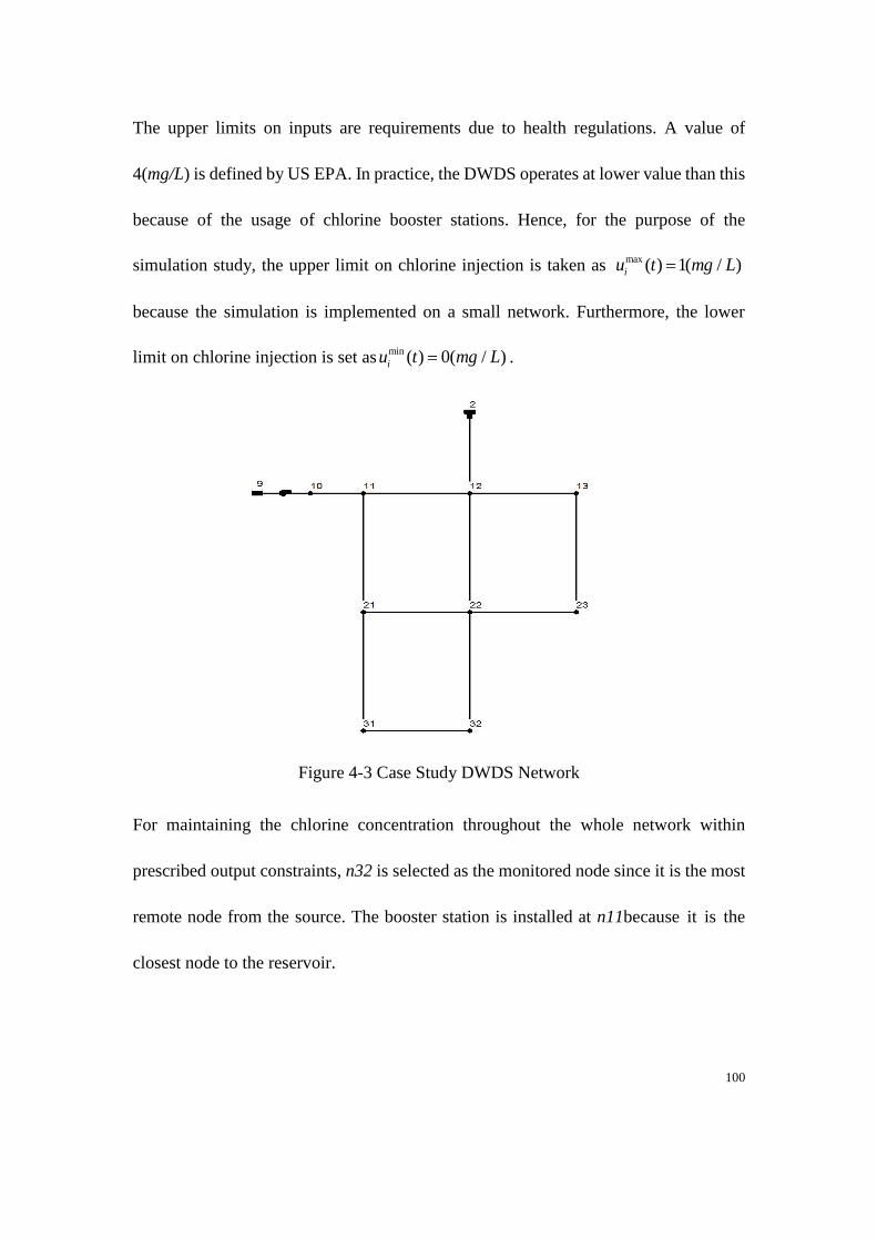
100
The upper limits on inputs are requirements due to health regulations. A value of
4(mg/L) is defined by US EPA. In practice, the DWDS operates at lower value than this
because of the usage of chlorine booster stations. Hence, for the purpose of the
simulation study, the upper limit on chlorine injection is taken as max ( ) 1( / )iu t mg L
because the simulation is implemented on a small network. Furthermore, the lower
limit on chlorine injection is set asmin ( ) 0( / )iu t mg L .
Figure 4-3 Case Study DWDS Network
For maintaining the chlorine concentration throughout the whole network within
prescribed output constraints, n32 is selected as the monitored node since it is the most
remote node from the source. The booster station is installed at n11because it is the
closest node to the reservoir.
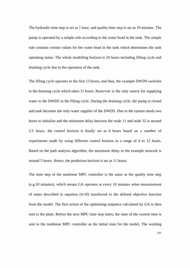
101
The hydraulic time step is set as 1 hour, and quality time step is set as 10 minutes. The
pump is operated by a simple rule according to the water head in the tank. The simple
rule contains certain values for the water head in the tank which determines the tank
operating status. The whole modelling horizon is 24 hours including filling cycle and
draining cycle due to the operation of the tank.
The filling cycle operates in the first 13 hours, and then, the example DWDS switches
to the draining cycle which takes 11 hours. Reservoir is the only source for supplying
water to the DWDS in the filling cycle. During the draining cycle, the pump is closed
and tank becomes the only water supplier of the DWDS. Due to the system needs two
hours to initialise and the minimum delay between the node 11 and node 32 is around
2.5 hours, the control horizon is finally set as 6 hours based on a number of
experiments made by using different control horizon in a range of 4 to 12 hours.
Based on the path analysis algorithm, the maximum delay in the example network is
around 5 hours. Hence, the prediction horizon is set as 11 hours.
The time step of the nonlinear MPC controller is the same as the quality time step
(e.g.10 minutes), which means GA operates at every 10 minutes when measurement
of states described in equation (4-10) transferred to the defined objective function
from the model. The first action of the optimising sequence calculated by GA is then
sent to the plant. Before the next MPC time step starts, the state of the current time is
sent to the nonlinear MPC controller as the initial state for the model. The working
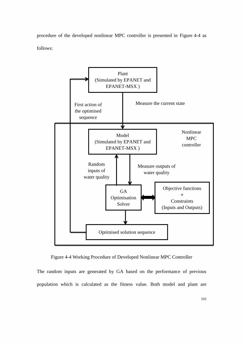
102
procedure of the developed nonlinear MPC controller is presented in Figure 4-4 as
follows:
Figure 4-4 Working Procedure of Developed Nonlinear MPC Controller
The random inputs are generated by GA based on the performance of previous
population which is calculated as the fitness value. Both model and plant are
Plant
(Simulated by EPANET and
EPANET-MSX )
Model
(Simulated by EPANET and
EPANET-MSX )
GA
Optimisation
Solver
Objective functions
+
Constraints
(Inputs and Outputs)
Measure the current state
Measure outputs of
water quality
Random
inputs of
water quality
Optimised solution sequence
First action of
the optimised
sequence
Nonlinear
MPC
controller

103
simulated by EPANET and EPANET-MSX but with different simulation data based
on the selected modelling horizon, control horizon and prediction horizon.
4.4.2 Software Implementation
The simulation is based on the MATLAB environment. The GA toolbox in MATLAB
is used to solve MPC optimising problems with connection to the EPANET software
package and EPANET Multi-Species Extension (MSX) module.
The MPC controller is running by each quality time step, as is the GA optimiser.
Therefore, in order to increase the optimiser computing efficiency, the optimised
population obtained at current time step is to be used as the initial population for the
next time step.
4.4.3 Simulation Results
As shown in the Figure 4-5, the trajectory of chlorine concentration at the monitored
node is maintained within the upper and lower limits. Figure 4-6 illustrates the
trajectory of minimised DBP concentration at the monitored node. Due to the system is
controlled under zero initial condition at junction nodes, there is no output comes out
in the first two hours because of initialising of the system. The output illustrated in
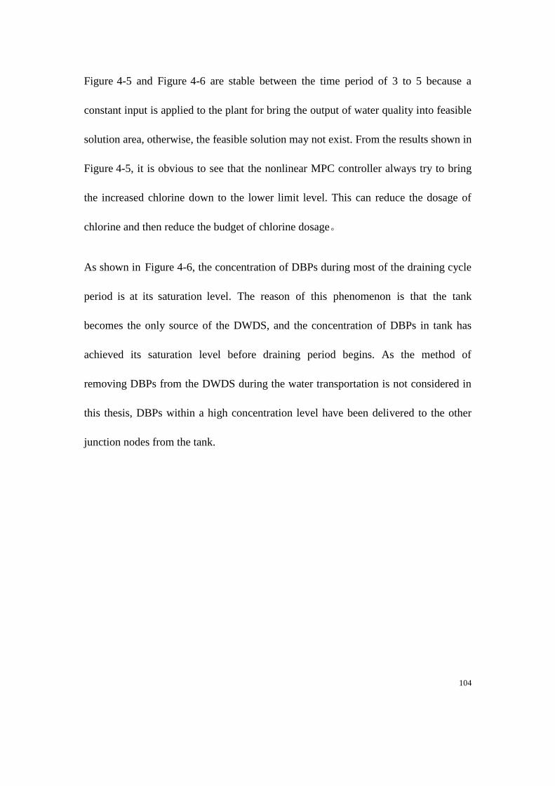
104
Figure 4-5 and Figure 4-6 are stable between the time period of 3 to 5 because a
constant input is applied to the plant for bring the output of water quality into feasible
solution area, otherwise, the feasible solution may not exist. From the results shown in
Figure 4-5, it is obvious to see that the nonlinear MPC controller always try to bring
the increased chlorine down to the lower limit level. This can reduce the dosage of
chlorine and then reduce the budget of chlorine dosage。
As shown in Figure 4-6, the concentration of DBPs during most of the draining cycle
period is at its saturation level. The reason of this phenomenon is that the tank
becomes the only source of the DWDS, and the concentration of DBPs in tank has
achieved its saturation level before draining period begins. As the method of
removing DBPs from the DWDS during the water transportation is not considered in
this thesis, DBPs within a high concentration level have been delivered to the other
junction nodes from the tank.
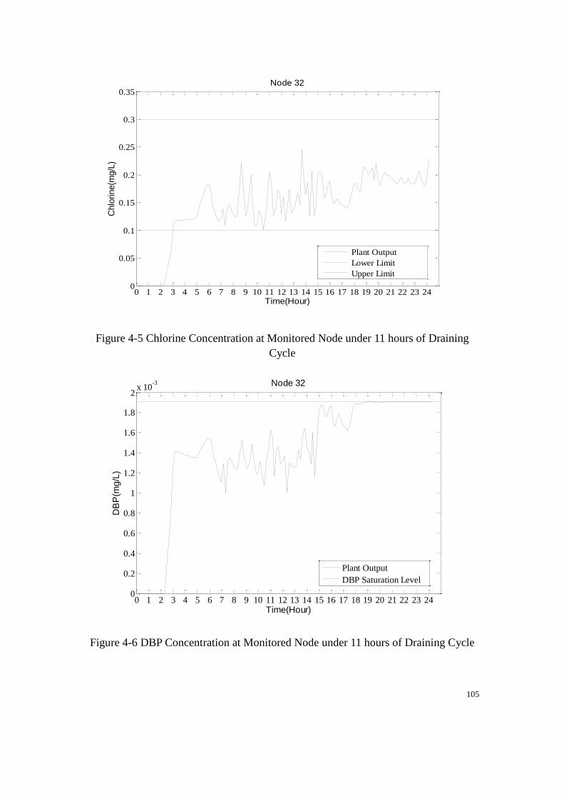
105
Figure 4-5 Chlorine Concentration at Monitored Node under 11 hours of Draining
Cycle
Figure 4-6 DBP Concentration at Monitored Node under 11 hours of Draining Cycle
0 1 2 3 4 5 6 7 8 9 10 11 12 13 14 15 16 17 18 19 20 21 22 23 240
0.05
0.1
0.15
0.2
0.25
0.3
0.35
Time(Hour)
Chlo
rine(m
g/L
)
Node 32
Plant Output
Lower Limit
Upper Limit
0 1 2 3 4 5 6 7 8 9 10 11 12 13 14 15 16 17 18 19 20 21 22 23 240
0.2
0.4
0.6
0.8
1
1.2
1.4
1.6
1.8
2x 10
-3
Time(Hour)
DB
P(m
g/L
)
Node 32
Plant Output
DBP Saturation Level
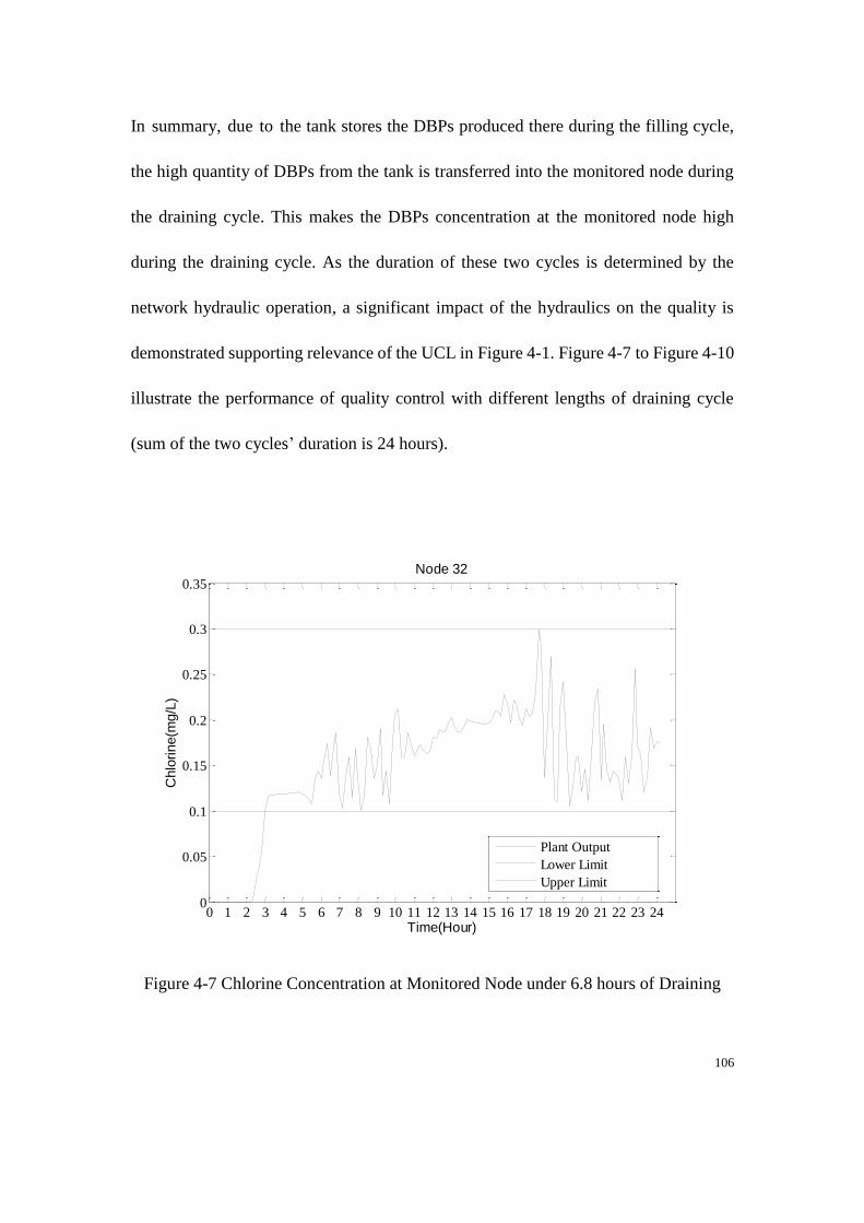
106
In summary, due to the tank stores the DBPs produced there during the filling cycle,
the high quantity of DBPs from the tank is transferred into the monitored node during
the draining cycle. This makes the DBPs concentration at the monitored node high
during the draining cycle. As the duration of these two cycles is determined by the
network hydraulic operation, a significant impact of the hydraulics on the quality is
demonstrated supporting relevance of the UCL in Figure 4-1. Figure 4-7 to Figure 4-10
illustrate the performance of quality control with different lengths of draining cycle
(sum of the two cycles’ duration is 24 hours).
Figure 4-7 Chlorine Concentration at Monitored Node under 6.8 hours of Draining
0 1 2 3 4 5 6 7 8 9 10 11 12 13 14 15 16 17 18 19 20 21 22 23 240
0.05
0.1
0.15
0.2
0.25
0.3
0.35
Time(Hour)
Chlo
rine(m
g/L
)
Node 32
Plant Output
Lower Limit
Upper Limit
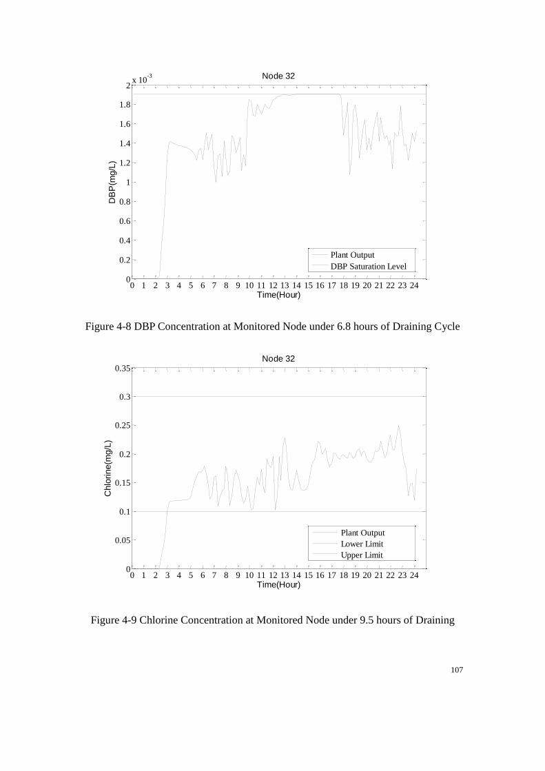
107
Figure 4-8 DBP Concentration at Monitored Node under 6.8 hours of Draining Cycle
Figure 4-9 Chlorine Concentration at Monitored Node under 9.5 hours of Draining
0 1 2 3 4 5 6 7 8 9 10 11 12 13 14 15 16 17 18 19 20 21 22 23 240
0.2
0.4
0.6
0.8
1
1.2
1.4
1.6
1.8
2x 10
-3
Time(Hour)
DB
P(m
g/L
)
Node 32
Plant Output
DBP Saturation Level
0 1 2 3 4 5 6 7 8 9 10 11 12 13 14 15 16 17 18 19 20 21 22 23 240
0.05
0.1
0.15
0.2
0.25
0.3
0.35
Time(Hour)
Chlo
rine(m
g/L
)
Node 32
Plant Output
Lower Limit
Upper Limit
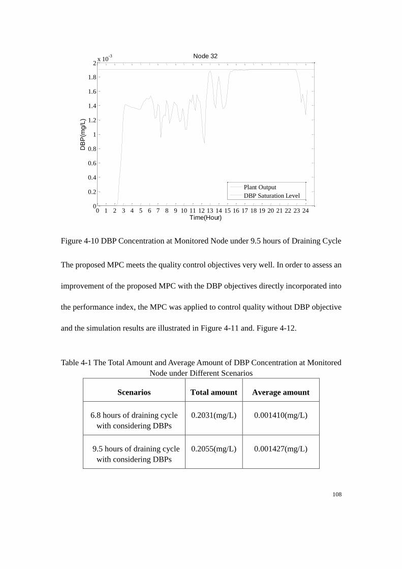
108
Figure 4-10 DBP Concentration at Monitored Node under 9.5 hours of Draining Cycle
The proposed MPC meets the quality control objectives very well. In order to assess an
improvement of the proposed MPC with the DBP objectives directly incorporated into
the performance index, the MPC was applied to control quality without DBP objective
and the simulation results are illustrated in Figure 4-11 and. Figure 4-12.
Table 4-1 The Total Amount and Average Amount of DBP Concentration at Monitored
Node under Different Scenarios
Scenarios Total amount Average amount
6.8 hours of draining cycle
with considering DBPs
0.2031(mg/L) 0.001410(mg/L)
9.5 hours of draining cycle
with considering DBPs
0.2055(mg/L) 0.001427(mg/L)
0 1 2 3 4 5 6 7 8 9 10 11 12 13 14 15 16 17 18 19 20 21 22 23 240
0.2
0.4
0.6
0.8
1
1.2
1.4
1.6
1.8
2x 10
-3
Time(Hour)
DB
P(m
g/L
)
Node 32
Plant Output
DBP Saturation Level
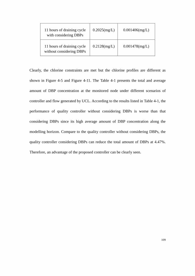
109
11 hours of draining cycle
with considering DBPs
0.2025(mg/L) 0.001406(mg/L)
11 hours of draining cycle
without considering DBPs
0.2128(mg/L) 0.001478(mg/L)
Clearly, the chlorine constraints are met but the chlorine profiles are different as
shown in Figure 4-5 and Figure 4-11. The Table 4-1 presents the total and average
amount of DBP concentration at the monitored node under different scenarios of
controller and flow generated by UCL. According to the results listed in Table 4-1, the
performance of quality controller without considering DBPs is worse than that
considering DBPs since its high average amount of DBP concentration along the
modelling horizon. Compare to the quality controller without considering DBPs, the
quality controller considering DBPs can reduce the total amount of DBPs at 4.47%.
Therefore, an advantage of the proposed controller can be clearly seen.
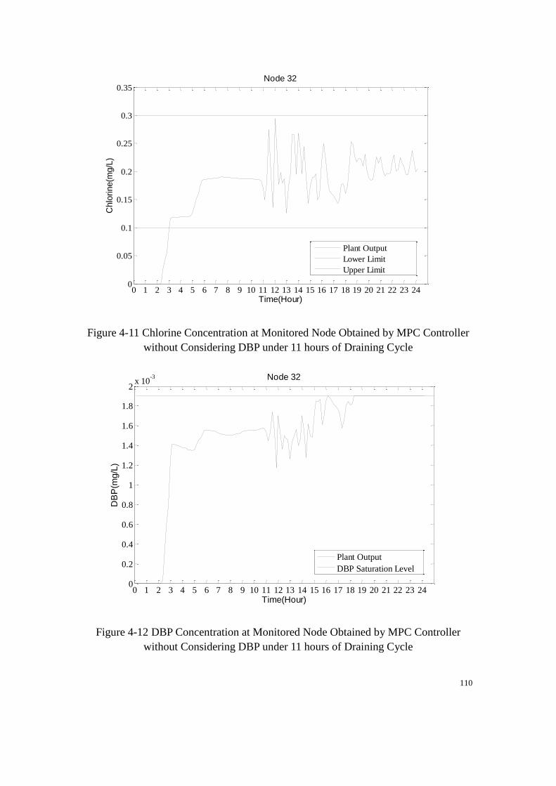
110
Figure 4-11 Chlorine Concentration at Monitored Node Obtained by MPC Controller
without Considering DBP under 11 hours of Draining Cycle
Figure 4-12 DBP Concentration at Monitored Node Obtained by MPC Controller
without Considering DBP under 11 hours of Draining Cycle
0 1 2 3 4 5 6 7 8 9 10 11 12 13 14 15 16 17 18 19 20 21 22 23 240
0.05
0.1
0.15
0.2
0.25
0.3
0.35
Time(Hour)
Chlo
rine(m
g/L
)
Node 32
Plant Output
Lower Limit
Upper Limit
0 1 2 3 4 5 6 7 8 9 10 11 12 13 14 15 16 17 18 19 20 21 22 23 240
0.2
0.4
0.6
0.8
1
1.2
1.4
1.6
1.8
2x 10
-3
Time(Hour)
DB
P(m
g/L
)
Node 32
Plant Output
DBP Saturation Level
111
4.5 Summary
This chapter has developed the nonlinear MPC control of water quality in DWDS
based on the advanced non-linear water quality dynamics model considering DBPs
objective. MPC has been considered as the control algorithm because it is widely used
in solving such nonlinear, constrained with multivariable problem. The basic
algorithm for MPC has been introduced and its application to a case study DWDS
network has been implemented. This nonlinear MPC controller provided a practical
solution for on-line control of water quality in DWDS considering DBPs. The
simulation results illustrated regarding to the nonlinear MPC application on water
quality control in DWDS have been shown a good and sustainable performance at
LCL with the fast quality feedback. Furthermore, an importance of the hydraulic
support as the quality control input was demonstrated.

112
CHAPTER 5 ROBUST PARAMETER
ESTIMATION AND OUTPUT PREDICTION ON
NONLINEAR WATER QUALITY MODEL IN
DWDS WITH CONSIDERING DBPS
Chapter 4 developed a nonlinear MPC controller based on nonlinear water quality
model which is modelled by EPANET and EPANET-MSX simulators. However, the
uncertainty is not considered in these simulators. Because uncertainty can be
explained by bounded parameters in the nonlinear water quality model, it is really
important to derive a bounded parameter model with uncertainty considered.
This chapter mainly describes the implementation of robust parameter estimation and
output prediction advanced algorithm based on nonlinear water quality model for the
purpose of estimating and predicting the water quality states in DWDS. The advanced
algorithm was tested for robustly predicting the outputs of a nonlinear water quality
model in DWDS incorporating DBPs. The application of point-parametric model
(PPM) for robustly estimating parameters of a nonlinear water quality model
considering DBPs by utilising multi-input multi-output (MIMO) model structure is
stretched.
113
The piece-wise constant parameters within the time-varying parameter model structure
explaining the dynamics of water quality considering DBPs in DWDS under input
disturbance is acquired by applying modified piece-wise continuity algorithms. This
chapter describes the robustness of the PPM framework on MIMO nonlinear water
quality model under multi-hydraulic operation status with advanced operating
procedures. The developed MIMO Point-Parametric Model is utilised to present
uncertainty and structure error in the nonlinear water quality model
5.1 Introduction
Climate change has a significant impact on continually growing systems, i.e. highly
complex and interconnected systems, such as power systems, transportation systems,
social networks, and drinking water systems, which are commonly known as a special
group of large-scale complex systems, namely critical infrastructure systems (CIS)
[167]. Some of the CIS, e.g. power grids and DWDS, constitute one group of systems
that can be described as reactive carrier-load nonlinear dynamic networks systems
(RCLNDNS) [167]. The monitoring, control and security of RCLNDNS-CIS has been
given great attention by both academics and industries for security and protection
purposes since September 11, 2011.
114
MPC technology has been widely applied in RCLNDNS-CIS to achieve complex
control objectives. However, in terms of nonlinear MPC, it is still insufficient to solve
those special defined optimisation tasks. This is the main reason that the control
strategies based on linear MPC become attractive while the internal model of linear
MPC still has large inaccuracies with regards to a real plant.
Managing MPC internal models working with uncertainties in the structure, unknown
parameters, and complex varying operational conditions has become the most crucial
task which requires proper mechanisms to guarantee the feasibility and veracity of the
internal models at all times. The application of PPM is expanded from multi-input
single-output (MISO) into multi-input multi-output (MIMO) because DBPs is
considered in this thesis and its piece-wise continuity advanced algorithm is then
further modified to be suitable for the MPC mechanism, especially for a robustly
feasible model predictive control (RFMPC) framework.
DWDS, as a typical RCLNDNS-CIS, are highly nonlinear systems not only because of
the multiple time-scale dynamics between the quantity operation and quality dynamics
[17, 18] but also due to the complex biochemical process which contains consuming
bacteria and limits its re-growth, the decay of disinfectant, and generation of DBPs
[161].
115
The characteristics listed above makes DWDS a good selection for investigating such
robust parameter estimation and output prediction technology for the purpose of
achieving the application of RFMPC on the nonlinear systems. In order to achieve a
proper working PPM, hydraulic information and the DWDS quality states including
both free chlorine concentration (disinfectant) and DBPs is required on-line. Robust
monitoring chlorine concentration in DWDS was well developed in [92], while the
quality monitoring with DBPs was presented in [7].
An PPM based approach utilised to deliver a linear structure quality model with
time-varying parameters and the related algorithms for robustly estimating parameters
and predicting outputs were presented in [2]. The structure of PPM was developed by
applying backward path tracking algorithm, described in Chapter 2.
5.2 MIMO Structure of PPM in IO Model
5.2.1 IO model of water quality in DWDS with Considering DBPs
The entire junction nodes and storage equipment in the DWDS are contained in the
water quality model and result in a distributed model within pipe transportation. In fact,
no explicit relationship exists between the chlorine injections and the concentrations of

116
chlorine and DBPs at the monitoring nodes in the DWDS, which represent the inputs
and outputs of the system in terms of water quality control.
As described in Chapter 4, the nonlinear water quality model used for the MPC
controller is modelled by EPANET simulator. However, for designing a control
system, an explicit relationship between the inputs and outputs is essential. As
presented in [2], the water quality transportation paths in the network and time delay
associated with paths connected between the injection nodes and monitored nodes were
calculated by applying a backward tracking algorithm, which was also known as the
path analysis for water quality transportation in the DWDS and described in the
previous.
Throughout the water quality transportation, chlorine consumes the bacteria and
generates decay. Furthermore, it reacts with organic matter in the water to generate
DBPs. Following that, both chlorine and DBPs mix with other flows at junction nodes,
the process of which is described by a series of impact coefficients in the final obtained
IO model. The time-delay existing in the input-output model which occurs due to the
transportation is time continuous and time varying.
In order to obtain the explicit IO water quality model with DBPs, the range of these
continuous time delays over the entire modelling horizon is discretized and
approximated by several delay numbers. The discrete IO model is normally obtained in
117
a moving average (MA) format. However, the existence of storage facilities increases
the detention time of water quality transportation from the input nodes to output nodes.
The increased detention time must be taken into consideration when processing the
dynamic of model. Therefore, the model parameters which can explain the quality
dynamics are required. The IO model with tanks in the DWDS is derived in an
autoregressive moving average (ARMA) format:
For Chlorine:
,
,
, , ,1 ,1 ,
1 ( )
,1
, ,1 ,1 , , ,1 ,1 ,
1 1 ( )
( ) ( ) ( ), S
( )
( ) ( ) ( ) ( ) ( ), S
1,...,
I
n j
T I
n j
n
n j i j n n f
j i I t
n n n
n h n n j i j n n d
h j i I t
M
a t u t i t t
y t
b t y t h a t u t i t t
for n n
(5-1)
For DBPs:
,
,
, , ,2 ,2 ,
1 ( )
,2
, ,2 ,1 , , ,2 ,2 ,
1 1 ( )
( ) ( ) ( ), S
( )
( ) ( ) ( ) ( ) ( ), S
1,...,
I
n j
T I
n j
n
n j i j n n f
j i I t
n n n
n h n n j i j n n d
h j i I t
M
a t u t i t t
y t
b t y t h a t u t i t t
for n n
(5-2)
where 0 0[ , ]Mt t t T ,
0t is the initial time and MT is the modelling horizon; ,1( )ny t
are chlorine concentrations and ,2 ( )ny t are DBPs concentration at the monitored node,
for 1,..., Mn n ; ( )ju t are chlorine concentrations at injection nodes, 1,..., Ij n ; Mn
118
and In present number of monitored nodes and number of injection nodes,
respectively; ,n fS and ,n dS present time-slots in filling and draining cycle,
respectively; , ( )n jI t denotes the delay number set that corresponds to output
,1 ,2( ) [ ( ), ( )]n n ny t y t y t associating with the thj input ( )ju t ;
, , , , ,1 , , ,2( ) [ ( ), ( )]n j i n j i n j ia t a t a t are the model parameters corresponding to the thn
output ( )ny t and the thj input ( )ju t associating with the delay number i ;
, , ,1 , ,2[ , ], 1,...,n h n h n h Tb b b h n are the parameters corresponding to the thn output
( )ny t that described dynamics caused by Tn tanks; ,,1 ,2( ) [ ( ) ( )]n n nt t t denotes
structure error in output ( )ny t .
5.2.2 MIMO Point-Parametric Model
5.2.2.1 Mathematical Model of MIMO Point-Parametric Model
Due to the fact that the IO model is discretized and linearized, the structure error is
inevitable and cannot be ignored. Meanwhile, the parameter uncertainty caused by
hydraulic information is unknown. Therefore, parameter estimation on bounding the
structure error and parameters is essential to build up a complete quality model for
control purposes.
The above IO model results in the discrete MIMO model structure:
119
,
,
,1 , ,1 ,1 , , ,1 ,1
1 1 ( )
,2 , ,2 ,1 , , ,2 ,2
1 1 ( )
( ) ( ) ( ) ( ) ( ) ( )
( ) ( ) ( ) ( ) ( ) ( )
1,...,
T I
n j
T I
n j
n n
n n h n n j i j n
h j i I k
n n
n n h n n j i j n
h j i I k
M
y k b k y k h a k u k i k
y k b k y k h a k u k i k
n n
(5-3)
Hence, the problem of parameter estimation is finally formulated as a time-varying
dynamic model in a form of MIMO with delayed inputs under uncertainty, which is
given as a general ARMA form:
,1 ,1 ,1
,2 ,2 ,2
1
1
n n n
n n n
y k k k k
y k k k k
(5-4)
Write above equations in a compact form yields:
0 01 , [ , ]n n n n m Zy k k k k k k k T (5-5)
where ,1 ,2( ) [ ( ), ( )]n n ny k y k y k denotes the outputs at thn monitored node; n k and
n k presents the model parameters and structure error, respectively, which explains
the uncertainties within the dynamics of the IO model; 1n k is the regressor
vector; 0k is the current time instant and
mT presents the modelling horizon length; Z
denotes the integer field. The structure of elements in (5-5) is shown as follows:
,1,1 , ,1 , ,1,1
,2 ,1,2 , ,2 , ,2
... ( ), [ ,..., ]
... ( )
T
T
n n n n In
n l u
n n n n n I
b k b k a kkk I i i
k b k b k a k
(5-6)
,1 ,1
1 , ,1 1 , ,1
, , , ,
1 [ ( 1),..., ( ),...
( ),... ( ),...
( ),... ( )]I I I I
n n n T
n l n u
n n l n n n u n
k y k y k n
u k i u k i
u k i u k i
(5-7)
120
,1 ,2[ , ]n n nk k k (5-8)
Actually, k can have a sudden change at time instant 0 0,j mk k k T , j Z ,
but the change can be considered to be very slow over a shorter time horizon 1,j jk k
and can be considered as constant during this shorter time horizon. Therefore, the
modelling time horizon Tm is partitioned into several time-slots [2] that results in the
following definition of the thj time-slot:
1: ,j j jS k Z k k k j Z
(5-9)
By using the data generated by the implicit model which is known as plant simulator,
the values build up the regressor, i.e. past measurements parameters, can be obtained.
The collection of the regressor under uncertainty in the model can be estimated by
using the bounding approach which is explained in [2]. However, since the structure
error is difficult to obtain in advance, it would be beneficial to bound parameters and
structure error and uncertainty together, which results in the application of PPM.
Then the union containing the entire model parameters that need to be searched is
expressed as:
0 0
, :
, ; ( ) , ,, , ,
1,..., , , ,
1,...,
E E E E E E
E E
n n n n n nn
n n n n n n
n nl u l ul u l u n n n n n n
n n n n
E E m Z
M
R y k k k
k
n N k k k T
n n
(5-10)
121
where ,n n k , and EN is the number of experiments required.
The final PPM structure is as follows:
0 0, , , , 1,...,
n n n n
n n m MZ
y k k k
k k k k T n n
(5-11)
The application of PPM on MIMO model structure is the main interest of this research
which results in jointly bounding the parameters within two outputs with interactions.
5.2.2.2 Structure of information exchange
The information exchange structure for explaining the PPM framework is shown in
Figure 5-1 [167]. The Calibrator is utilised for processing the initial information
containing parameters and measurements and delivering them to implicit model, i.e.
Plant Simulator in Figure 5-1 and build up plant information, i.e. Structure Information
in Figure 5-1. The essential data are redistributed between Plant Simulator, Estimator
and Explicit Model. The Model Structure Determination is required to establish the
Explicit Model structure. Based on the estimated model parameters, the Explicit Model
generates the robust output predictions, including output prediction of nominal model
in a form of Chebyshev Centre and upper & lower bounds for real plant. The clear
explanation of the aforementioned structure can be found in [167].
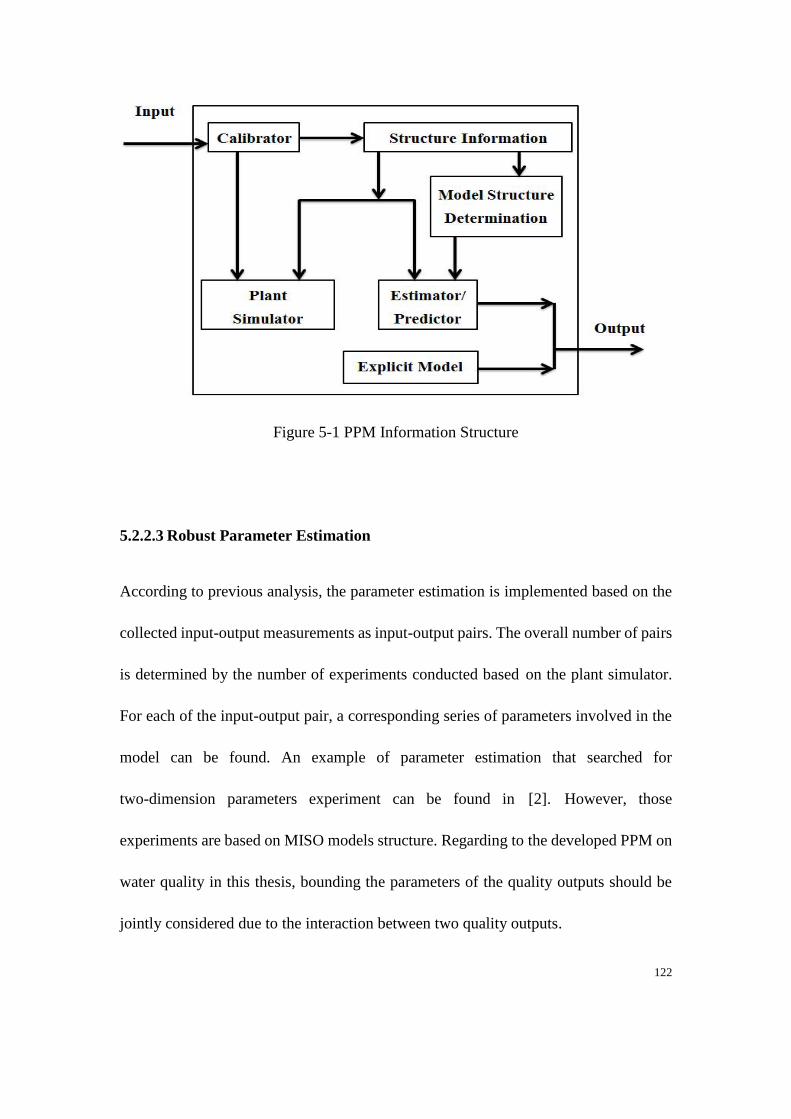
122
Figure 5-1 PPM Information Structure
5.2.2.3 Robust Parameter Estimation
According to previous analysis, the parameter estimation is implemented based on the
collected input-output measurements as input-output pairs. The overall number of pairs
is determined by the number of experiments conducted based on the plant simulator.
For each of the input-output pair, a corresponding series of parameters involved in the
model can be found. An example of parameter estimation that searched for
two-dimension parameters experiment can be found in [2]. However, those
experiments are based on MISO models structure. Regarding to the developed PPM on
water quality in this thesis, bounding the parameters of the quality outputs should be
jointly considered due to the interaction between two quality outputs.
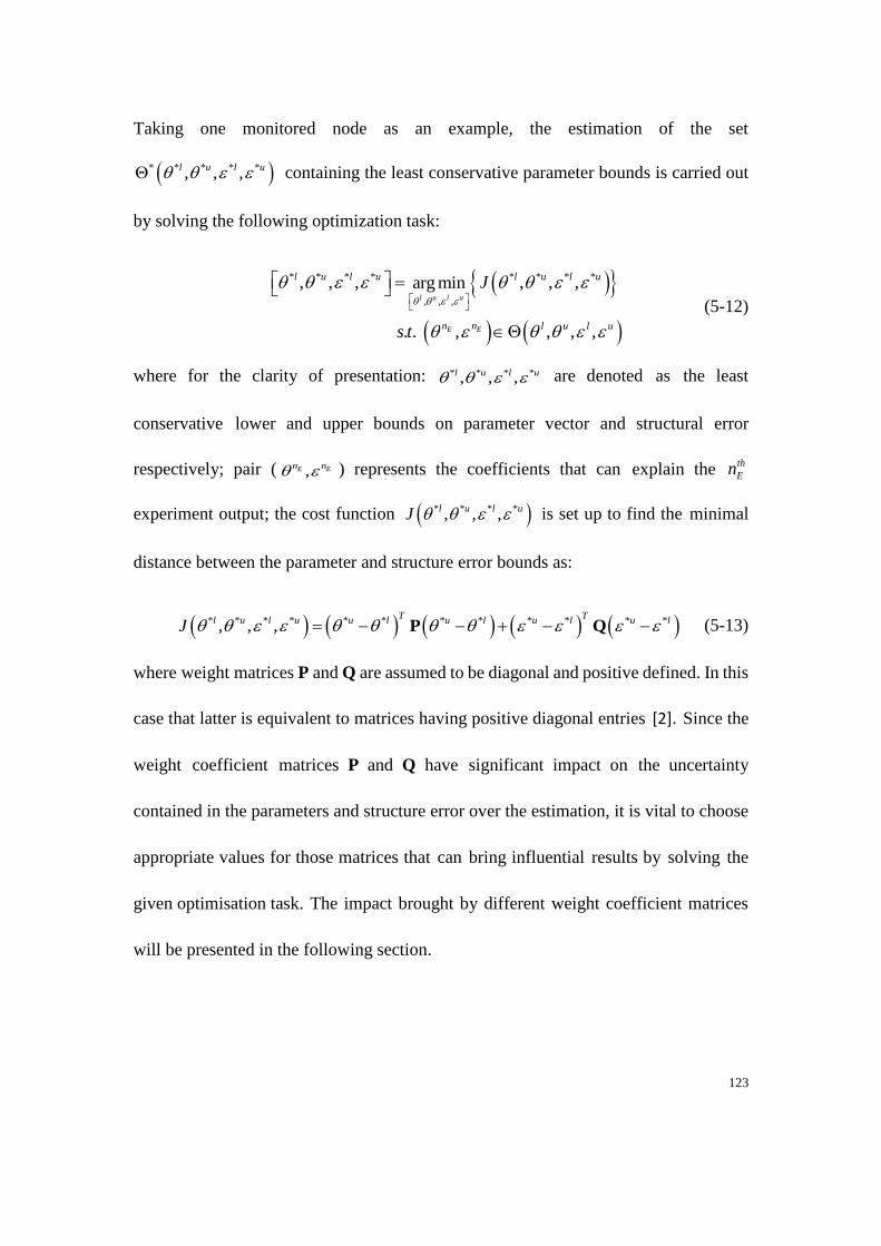
123
Taking one monitored node as an example, the estimation of the set
* * * * *, , ,l u l u containing the least conservative parameter bounds is carried out
by solving the following optimization task:
* * * * * * * *
, , ,
, , , , , ,arg min
. . , , , ,
l u l u
E E
l u l u l u l u
n n l u l u
J
s t
(5-12)
where for the clarity of presentation: * * * *, , ,l u l u are denoted as the least
conservative lower and upper bounds on parameter vector and structural error
respectively; pair ( ,E En n ) represents the coefficients that can explain the th
En
experiment output; the cost function * * * *, , ,l u l uJ is set up to find the minimal
distance between the parameter and structure error bounds as:
* * * * * * * * * * * *, , ,T T
l u l u u l u l u l u lJ P Q (5-13)
where weight matrices P and Q are assumed to be diagonal and positive defined. In this
case that latter is equivalent to matrices having positive diagonal entries [2]. Since the
weight coefficient matrices P and Q have significant impact on the uncertainty
contained in the parameters and structure error over the estimation, it is vital to choose
appropriate values for those matrices that can bring influential results by solving the
given optimisation task. The impact brought by different weight coefficient matrices
will be presented in the following section.
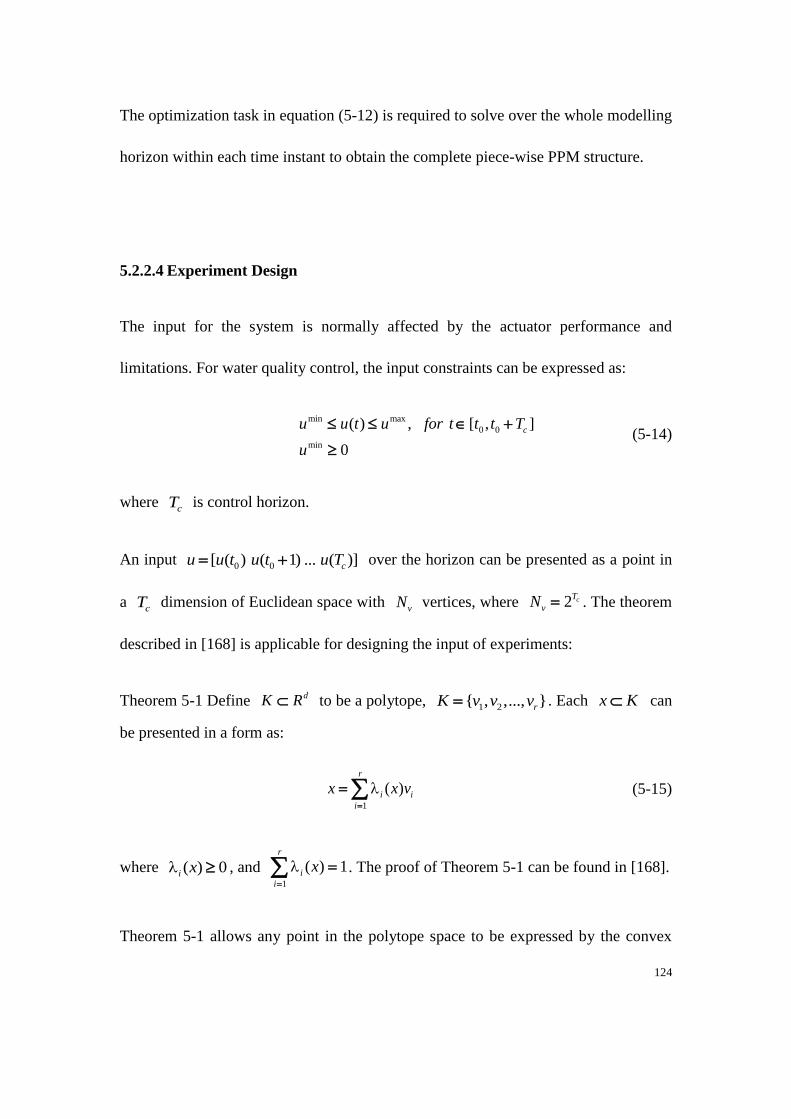
124
The optimization task in equation (5-12) is required to solve over the whole modelling
horizon within each time instant to obtain the complete piece-wise PPM structure.
5.2.2.4 Experiment Design
The input for the system is normally affected by the actuator performance and
limitations. For water quality control, the input constraints can be expressed as:
min max
0 0
min
( ) , [ , ]
0
cu u t u for t t t T
u
(5-14)
where cT is control horizon.
An input 0 0[ ( ) ( 1) ... ( )]cu u t u t u T over the horizon can be presented as a point in
a cT dimension of Euclidean space with
vN vertices, where 2 cT
vN . The theorem
described in [168] is applicable for designing the input of experiments:
Theorem 5-1 Define dK R to be a polytope,
1 2{ , ,..., }rK v v v . Each x K can
be presented in a form as:
1
( )r
i i
i
x x v
(5-15)
where ( ) 0i x , and 1
( ) 1r
i
i
x
. The proof of Theorem 5-1 can be found in [168].
Theorem 5-1 allows any point in the polytope space to be expressed by the convex
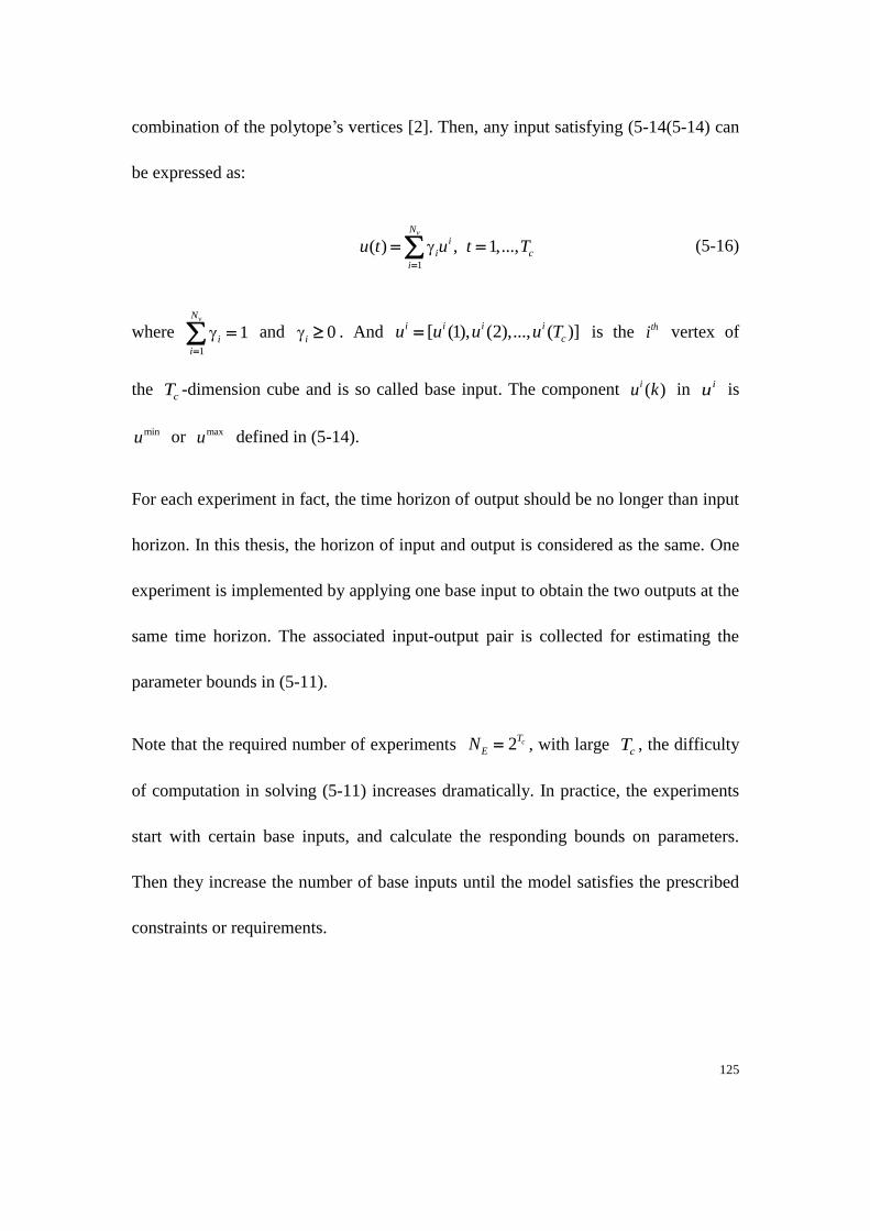
125
combination of the polytope’s vertices [2]. Then, any input satisfying (5-14(5-14) can
be expressed as:
1
( ) , 1,...,vN
i
i c
i
u t u t T
(5-16)
where 1
1vN
i
i
and 0i . And [ (1), (2),..., ( )]i i i i
cu u u u T is the thi vertex of
the cT -dimension cube and is so called base input. The component ( )iu k in iu is
minu or maxu defined in (5-14).
For each experiment in fact, the time horizon of output should be no longer than input
horizon. In this thesis, the horizon of input and output is considered as the same. One
experiment is implemented by applying one base input to obtain the two outputs at the
same time horizon. The associated input-output pair is collected for estimating the
parameter bounds in (5-11).
Note that the required number of experiments 2 cT
EN , with large cT , the difficulty
of computation in solving (5-11) increases dramatically. In practice, the experiments
start with certain base inputs, and calculate the responding bounds on parameters.
Then they increase the number of base inputs until the model satisfies the prescribed
constraints or requirements.
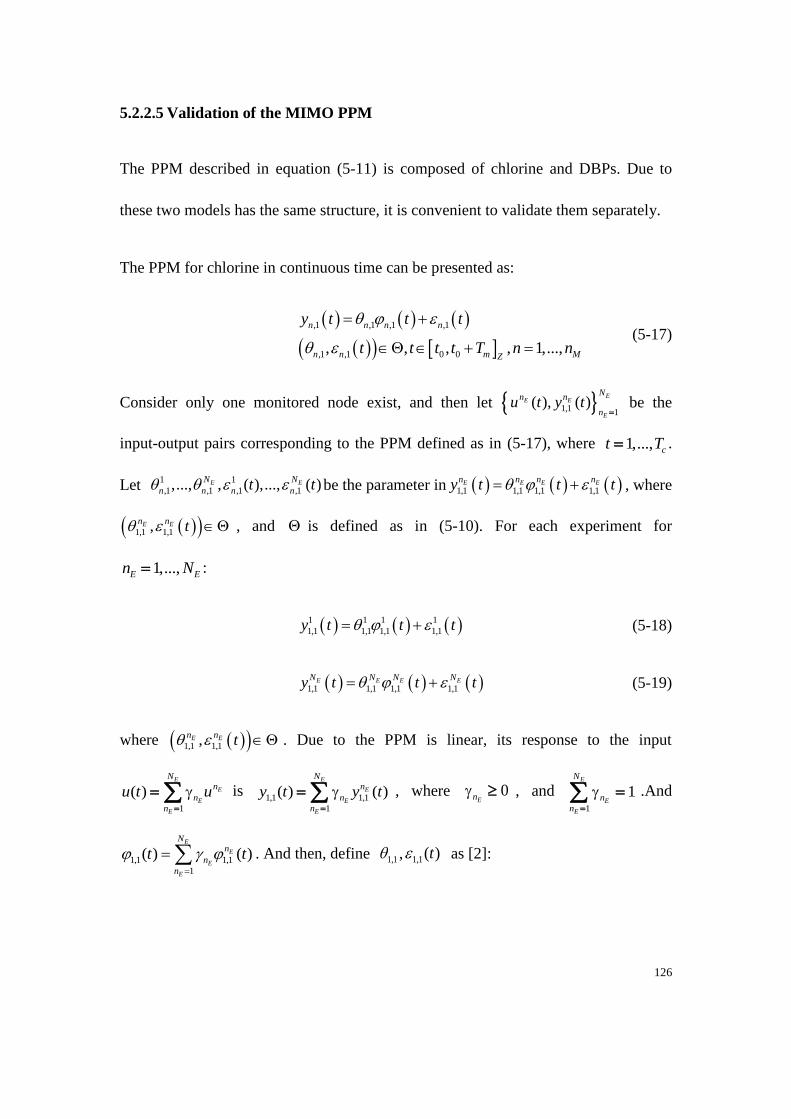
126
5.2.2.5 Validation of the MIMO PPM
The PPM described in equation (5-11) is composed of chlorine and DBPs. Due to
these two models has the same structure, it is convenient to validate them separately.
The PPM for chlorine in continuous time can be presented as:
,1 ,1 ,1 ,1
,1 ,1 0 0, , , , 1,...,
n n n n
n n m MZ
y t t t
t t t t T n n
(5-17)
Consider only one monitored node exist, and then let 1,1 1( ), ( )
EE E
E
Nn n
nu t y t
be the
input-output pairs corresponding to the PPM defined as in (5-17), where 1,..., ct T .
Let 1 1
,1 ,1 ,1 ,1,..., , ( ),..., ( )E EN N
n n n nt t be the parameter in 1,1 1,1 1,1 1,1E E E En n n n
y t t t , where
1,1 1,1,E En n t , and is defined as in (5-10). For each experiment for
1,...,E En N :
1 1 1 1
1,1 1,1 1,1 1,1y t t t (5-18)
1,1 1,1 1,1 1,1E E E EN N N N
y t t t (5-19)
where 1,1 1,1,E En n t . Due to the PPM is linear, its response to the input
1
( )E
E
E
E
Nn
n
n
u t u
is 1,1 1,1
1
( ) ( )E
E
E
E
Nn
n
n
y t y t
, where 0En , and
1
1E
E
E
N
n
n
.And
1,1 1,1
1
( ) ( )E
E
E
E
Nn
n
n
t t
. And then, define 1,1 , 1,1( )t as [2]:
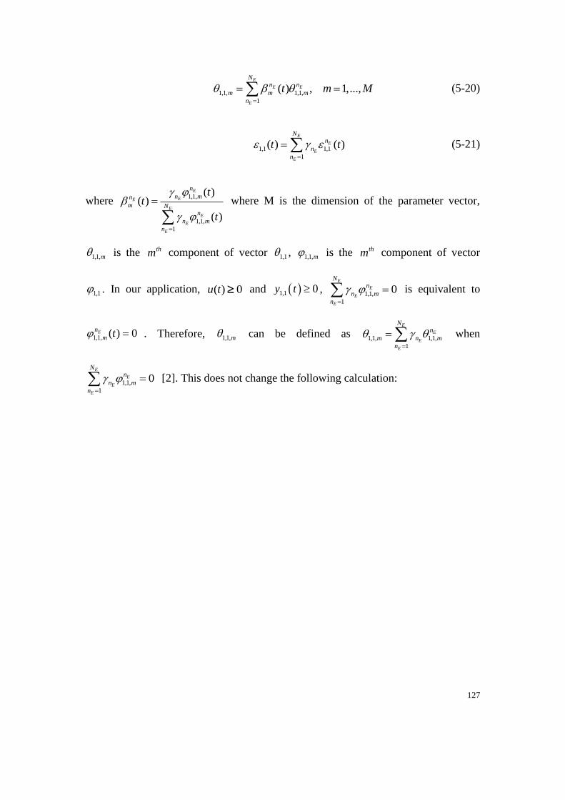
127
1,1, 1,1,
1
( ) , 1,...,E
E E
E
Nn n
m m m
n
t m M
(5-20)
1,1 1,1
1
( ) ( )E
E
E
E
Nn
n
n
t t
(5-21)
where 1,1,
1,1,
1
( )( )
( )
E
EE
E
E
E
E
n
n mn
m Nn
n m
n
tt
t
where M is the dimension of the parameter vector,
1,1,m is the thm component of vector 1,1 , 1,1,m is the thm component of vector
1,1 . In our application, ( ) 0u t and 1,1 0y t , 1,1,
1
0E
E
E
E
Nn
n m
n
is equivalent to
1,1, ( ) 0En
m t . Therefore, 1,1,m can be defined as 1,1, 1,1,
1
E
E
E
E
Nn
m n m
n
when
1,1,
1
0E
E
E
E
Nn
n m
n
[2]. This does not change the following calculation:
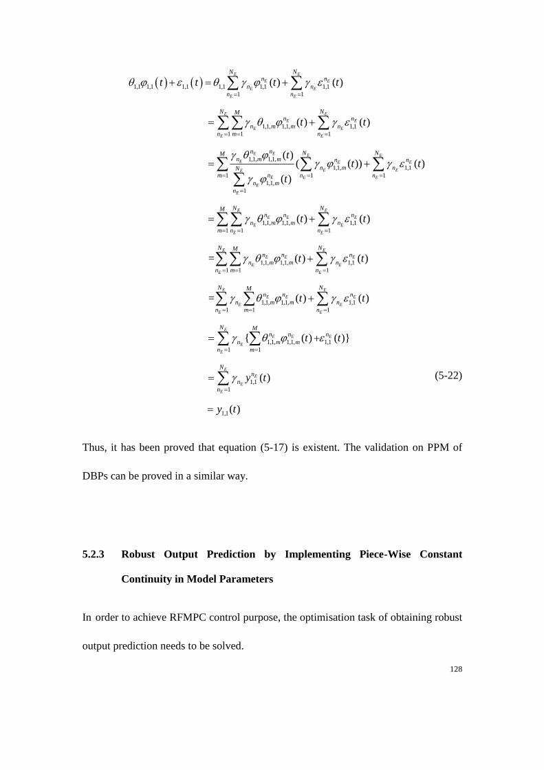
128
1,1 1,1 1,1 1,1 1,1 1,1
1 1
1,1, 1,1, 1,1
1 1 1
1,1, 1,1,
1,1, 1,1
1 1
1,1,
1
( ) ( )
( ) ( )
( )( ( )) ( )
( )
E E
E E
E E
E E
E E
E E
E E
E E
E E E
E E E
E EE
E E E
E
E
N Nn n
n n
n n
N NMn n
n m m n
n m n
n n NMn m m n n
n m nNnm n n
n m
n
t t t t
t t
tt t
t
1
1,1, 1,1, 1,1
1 1 1
1,1, 1,1, 1,1
1 1 1
1,1, 1,1, 1,1
1 1 1
1,1, 1,1,
1
( ) ( )
= ( ) ( )
= ( ) ( )
{ ( )
E
E E
E E E
E E
E E
E E
E E E
E E
E E
E E
E E E
E E
E E
E E
E
N
N NMn n n
n m m n
m n n
N NMn n n
n m m n
n m n
N NMn n n
n m m n
n m n
Mn n
n m m
n m
t t
t t
t t
t
1,1
1
1,1
1
1,1
( )}
( )
( )
E
E
E
E
E
E
E
Nn
Nn
n
n
t
y t
y t
(5-22)
Thus, it has been proved that equation (5-17) is existent. The validation on PPM of
DBPs can be proved in a similar way.
5.2.3 Robust Output Prediction by Implementing Piece-Wise Constant
Continuity in Model Parameters
In order to achieve RFMPC control purpose, the optimisation task of obtaining robust
output prediction needs to be solved.
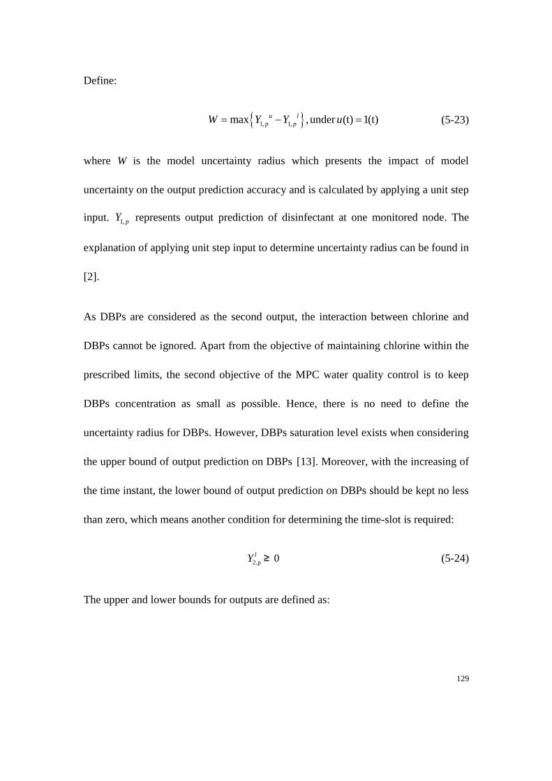
129
Define:
1, 1,max ,under (t) 1(t)u l
p pW Y Y u (5-23)
where W is the model uncertainty radius which presents the impact of model
uncertainty on the output prediction accuracy and is calculated by applying a unit step
input. 1, pY represents output prediction of disinfectant at one monitored node. The
explanation of applying unit step input to determine uncertainty radius can be found in
[2].
As DBPs are considered as the second output, the interaction between chlorine and
DBPs cannot be ignored. Apart from the objective of maintaining chlorine within the
prescribed limits, the second objective of the MPC water quality control is to keep
DBPs concentration as small as possible. Hence, there is no need to define the
uncertainty radius for DBPs. However, DBPs saturation level exists when considering
the upper bound of output prediction on DBPs [13]. Moreover, with the increasing of
the time instant, the lower bound of output prediction on DBPs should be kept no less
than zero, which means another condition for determining the time-slot is required:
2,p 0lY ≥ (5-24)
The upper and lower bounds for outputs are defined as:
130
1, 2,
1| |
1| |
[ , ]
u u u
p p p m
l l l
p p p m
p p p
Y y k k y k T k
Y y k k y k T k
where Y Y Y
(5-25)
where 1|u
py k k and 1|u
py k k are calculated based on solving the following
optimisation problems [2]:
,
,
| max |
. . |
| min |
. . |
p t i
p k i
u
pV
p
l
pV
p
y k i k y k i k
s t y k i k Y
y k i k y k i k
s t y k i k Y
(5-26)
where ,p t iV is given by:
,
1| ,.., | ,
1| ,.., | ,
, 1| ,.., |
p k i
y k t y k i t
V k t k i t
k t k i t
(5-27)
The robust output prediction is calculated by the following algorithm: A priori
partitioning is produced based on the path analysis;
Step 2. Starting estimation at t0 with N=1, the parameter bounds are calculated
by solving Equation (5-16);
Step 3. If 0t N is within the a priori slot and corresponding obtained W
satisfies with the selected Wmax and Equation (5-24) is satisfied, set
N=N+1, back to Step 2;
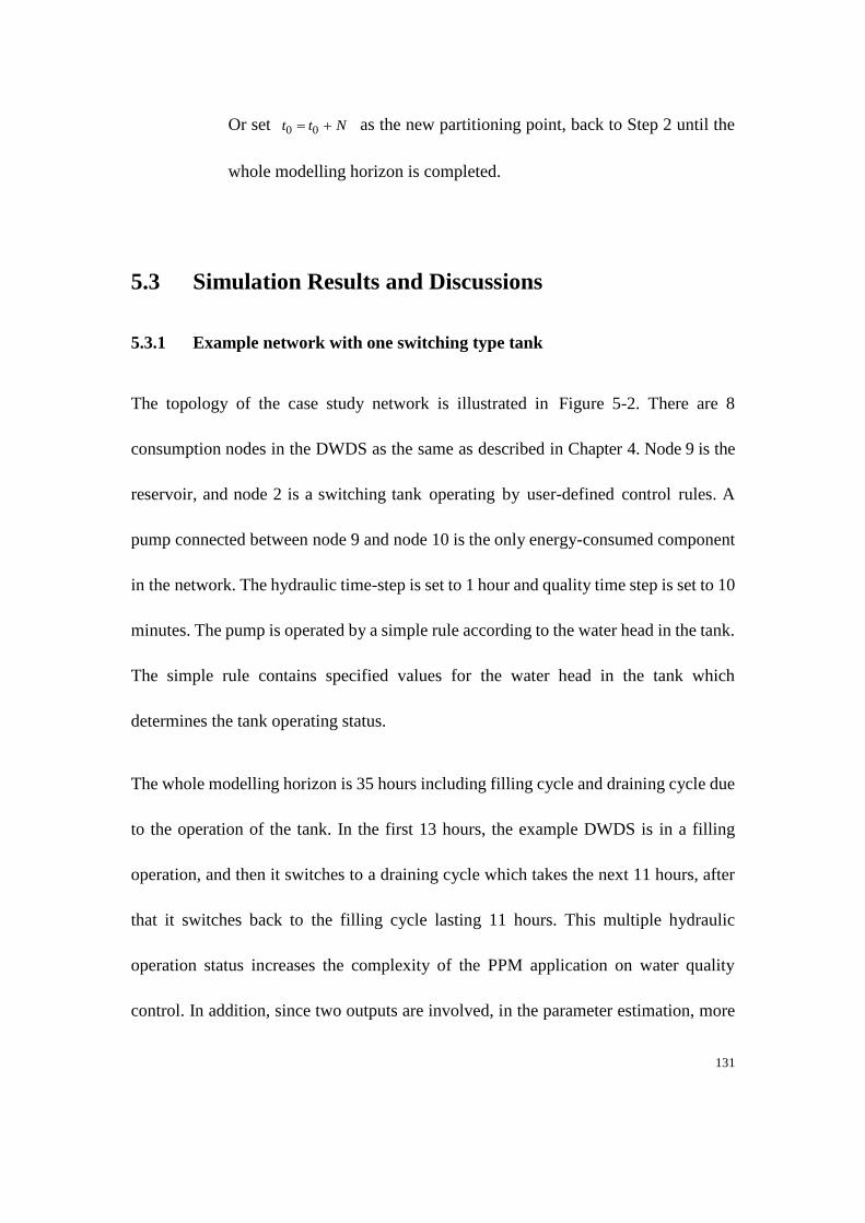
131
Or set 0 0t t N as the new partitioning point, back to Step 2 until the
whole modelling horizon is completed.
5.3 Simulation Results and Discussions
5.3.1 Example network with one switching type tank
The topology of the case study network is illustrated in Figure 5-2. There are 8
consumption nodes in the DWDS as the same as described in Chapter 4. Node 9 is the
reservoir, and node 2 is a switching tank operating by user-defined control rules. A
pump connected between node 9 and node 10 is the only energy-consumed component
in the network. The hydraulic time-step is set to 1 hour and quality time step is set to 10
minutes. The pump is operated by a simple rule according to the water head in the tank.
The simple rule contains specified values for the water head in the tank which
determines the tank operating status.
The whole modelling horizon is 35 hours including filling cycle and draining cycle due
to the operation of the tank. In the first 13 hours, the example DWDS is in a filling
operation, and then it switches to a draining cycle which takes the next 11 hours, after
that it switches back to the filling cycle lasting 11 hours. This multiple hydraulic
operation status increases the complexity of the PPM application on water quality
control. In addition, since two outputs are involved, in the parameter estimation, more
132
estimated parameters are introduced, which further increases the complexity of the
application of PPM on MIMO.
Figure 5-3 The Case Study Network with a Switching Tank
The junction node n32 is selected as the monitored node since its location is considered
to be the most remote from the source. The booster station is installed at n11 (Injection
node). The algorithms on determining allocation of booster stations are presented in [71,
74].
The constraints of control input in this network can be expressed as:
0(mg/ L) ( ) 1(mg/ L), [0, ]mu t for t T (5-28)
133
5.3.2 Illustration of Path Analysis Algorithm
The IO model of water quality is described by equations (5-2) and (5-3). During the
filling cycle, three paths are active from the injection node to the monitored node,
which can be denoted by the sequences of the pipe ID, i.e. Path I (111-121-31), Path II
(111-21-122), and Path III (11-112-122). Only one path is active when the tank
switches to the draining period which is Path I. Algorithms of calculating the detention
time of quality transportation in DWDS were described in Chapter 3. The water quality
transportation delay in paths and associated delay number can be calculated by
applying a backward tracking algorithm, and the tracking time step is set to 1 minute.
The path analysis result is shown in Figure 5-4. Figure 5-5 illustrates the time delay in 3
active paths. The delay number corresponding to the associated paths can be calculated.
The simulation is based on MATLAB with a connection to EPANET software package
and EPANET Multi-Species (MSX) Module.
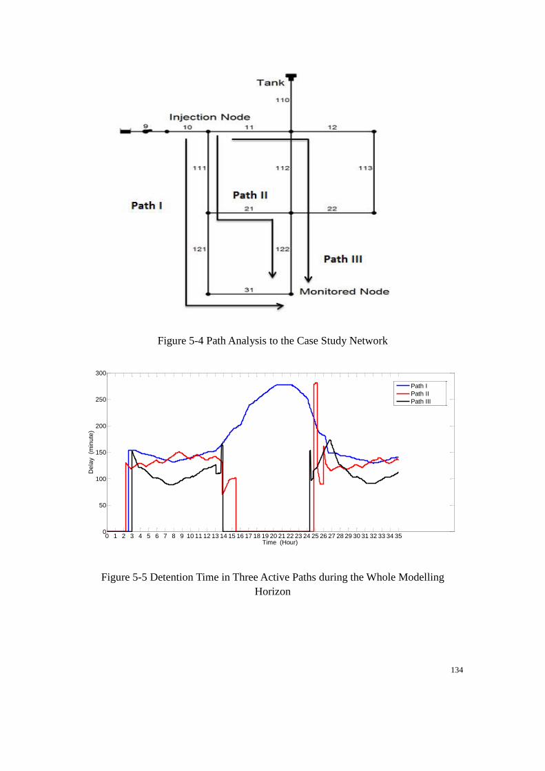
134
Figure 5-4 Path Analysis to the Case Study Network
Figure 5-5 Detention Time in Three Active Paths during the Whole Modelling
Horizon
0 1 2 3 4 5 6 7 8 9 10 11 12 13 14 15 16 17 18 19 20 21 22 23 24 25 26 27 28 29 30 31 32 33 34 350
50
100
150
200
250
300
Time (Hour)
De
lay
(min
ute
)
Path I
Path II
Path III
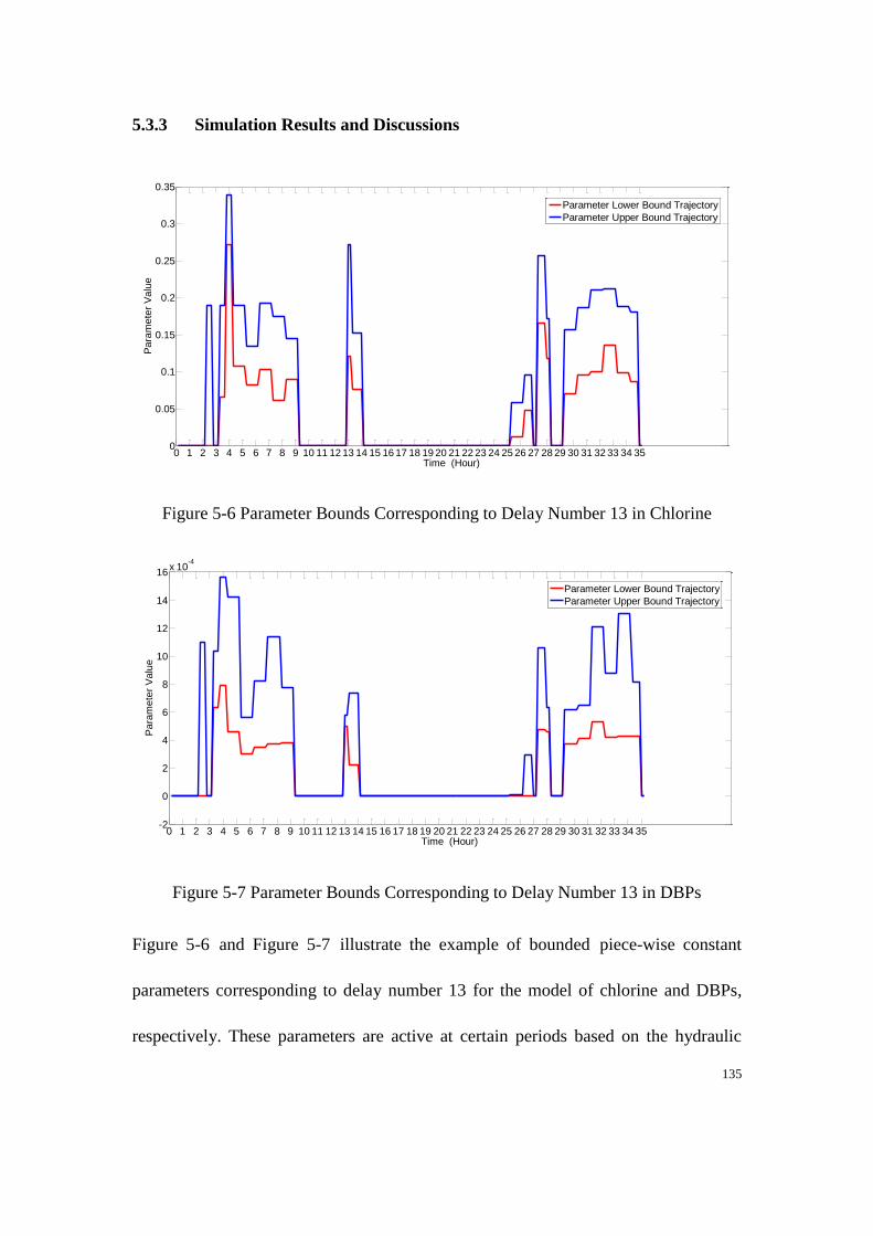
135
5.3.3 Simulation Results and Discussions
Figure 5-6 Parameter Bounds Corresponding to Delay Number 13 in Chlorine
Figure 5-7 Parameter Bounds Corresponding to Delay Number 13 in DBPs
Figure 5-6 and Figure 5-7 illustrate the example of bounded piece-wise constant
parameters corresponding to delay number 13 for the model of chlorine and DBPs,
respectively. These parameters are active at certain periods based on the hydraulic
0 1 2 3 4 5 6 7 8 9 10 11 12 13 14 15 16 17 18 19 20 21 22 23 24 25 26 27 28 29 30 31 32 33 34 350
0.05
0.1
0.15
0.2
0.25
0.3
0.35
Time (Hour)
Pa
ram
ete
r V
alu
e
Parameter Lower Bound Trajectory
Parameter Upper Bound Trajectory
0 1 2 3 4 5 6 7 8 9 10 11 12 13 14 15 16 17 18 19 20 21 22 23 24 25 26 27 28 29 30 31 32 33 34 35-2
0
2
4
6
8
10
12
14
16x 10
-4
Time (Hour)
Pa
ram
ete
r V
alu
e
Parameter Lower Bound Trajectory
Parameter Upper Bound Trajectory
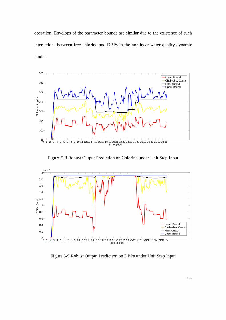
136
operation. Envelops of the parameter bounds are similar due to the existence of such
interactions between free chlorine and DBPs in the nonlinear water quality dynamic
model.
Figure 5-8 Robust Output Prediction on Chlorine under Unit Step Input
Figure 5-9 Robust Output Prediction on DBPs under Unit Step Input
0 1 2 3 4 5 6 7 8 9 10 11 12 13 14 15 16 17 18 19 20 21 22 23 24 25 26 27 28 29 30 31 32 33 34 350
0.1
0.2
0.3
0.4
0.5
0.6
0.7
Time (Hour)
Ch
lori
ne
(m
g/L
)
Lower Bound
Chebyshev Center
Plant Output
Upper Bound
0 1 2 3 4 5 6 7 8 9 10 11 12 13 14 15 16 17 18 19 20 21 22 23 24 25 26 27 28 29 30 31 32 33 34 350
0.2
0.4
0.6
0.8
1
1.2
1.4
1.6
1.8
2x 10
-3
Time (Hour)
DB
Ps
(mg
/L)
Lower Bound
Chebyshev Center
Plant Output
Upper Bound
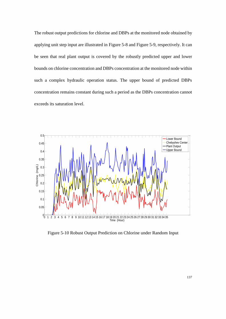
137
The robust output predictions for chlorine and DBPs at the monitored node obtained by
applying unit step input are illustrated in Figure 5-8 and Figure 5-9, respectively. It can
be seen that real plant output is covered by the robustly predicted upper and lower
bounds on chlorine concentration and DBPs concentration at the monitored node within
such a complex hydraulic operation status. The upper bound of predicted DBPs
concentration remains constant during such a period as the DBPs concentration cannot
exceeds its saturation level.
Figure 5-10 Robust Output Prediction on Chlorine under Random Input
0 1 2 3 4 5 6 7 8 9 10 11 12 13 14 15 16 17 18 19 20 21 22 23 24 25 26 27 28 29 30 31 32 33 34 350
0.05
0.1
0.15
0.2
0.25
0.3
0.35
0.4
0.45
0.5
Time (Hour)
Ch
lori
ne
(m
g/L
)
Lower Bound
Chebyshev Center
Plant Output
Upper Bound
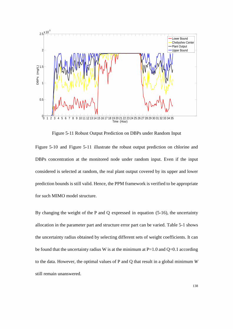
138
Figure 5-11 Robust Output Prediction on DBPs under Random Input
Figure 5-10 and Figure 5-11 illustrate the robust output prediction on chlorine and
DBPs concentration at the monitored node under random input. Even if the input
considered is selected at random, the real plant output covered by its upper and lower
prediction bounds is still valid. Hence, the PPM framework is verified to be appropriate
for such MIMO model structure.
By changing the weight of the P and Q expressed in equation (5-16), the uncertainty
allocation in the parameter part and structure error part can be varied. Table 5-1 shows
the uncertainty radius obtained by selecting different sets of weight coefficients. It can
be found that the uncertainty radius W is at the minimum at P=1.0 and Q=0.1 according
to the data. However, the optimal values of P and Q that result in a global minimum W
still remain unanswered.
0 1 2 3 4 5 6 7 8 9 10 11 12 13 14 15 16 17 18 19 20 21 22 23 24 25 26 27 28 29 30 31 32 33 34 350
0.5
1
1.5
2
2.5x 10
-3
Time (Hour)
DB
Ps
(mg
/L)
Lower Bound
Chebyshev Center
Plant Output
Upper Bound
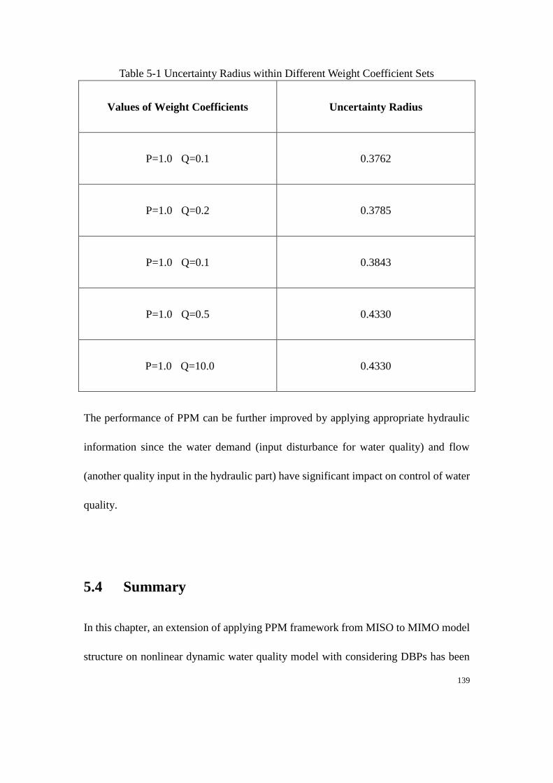
139
Table 5-1 Uncertainty Radius within Different Weight Coefficient Sets
Values of Weight Coefficients Uncertainty Radius
P=1.0 Q=0.1 0.3762
P=1.0 Q=0.2 0.3785
P=1.0 Q=0.1 0.3843
P=1.0 Q=0.5 0.4330
P=1.0 Q=10.0 0.4330
The performance of PPM can be further improved by applying appropriate hydraulic
information since the water demand (input disturbance for water quality) and flow
(another quality input in the hydraulic part) have significant impact on control of water
quality.
5.4 Summary
In this chapter, an extension of applying PPM framework from MISO to MIMO model
structure on nonlinear dynamic water quality model with considering DBPs has been
140
presented. The MISO output prediction algorithm has been incorporated with MIMO in
order to robustly estimate parameters of the quality model.
The piece-wise constant parameters for such a MIMO model have been obtained for the
purpose of robust feasible control on water quality considering DBPs. The explicit
structure of the water quality model has been also presented in the form of a
input-output model by implementing a back-tracking algorithm.
The simulation results above described the piece-wise constant parameters within the
MIMO PPM and also illustrated that the real plant outputs can be explained by their
upper and lower prediction bounds. In addition, this chapter has developed the MISO
model structure into the MIMO model structure. The capability of PPM of processing a
wider range of system identification problems has been proved. The importance of the
hydraulic support to the quality control has been highlighted. The MIMO model and the
algorithm presented in this chapter will be beneficial for robust feasible model
predictive control of water quality in DWDS considering DBPs.
141
CHAPTER 6 CONCLUSION AND FUTURE
RESEARCH WORK
6.1 Conclusions
Quantity and quality control are the two main interests in the operational control of
DWDS. The quality control problem has been discussed in this thesis within a newly
derived nonlinear water quality model. Compared to the linear water quality model,
the advanced nonlinear water quality model considering dynamic of DBPs is more
close to the real DWDS application. Objectives of the water quality control problem
have been replenished when considering the existences of DBPs. Conclusions for this
thesis are summarised as follows:
1. One of the main objectives in this thesis is to develop a nonlinear MPC
controller for optimising water quality in DWDS with DBPs under defined constraints.
Firstly, according to the work been done in Chapter 4, MPC has been proved as the
core control driver in solving such nonlinear, constrained, multivariable problem. This
nonlinear MPC controller successfully provided a practical solution for on-line
control of water quality in DWDS considering augmented DBPs objective.
Furthermore, the simulation results illustrated in Chapter 4 have been shown a good
142
MPC controller performance on dealing with water quality optimisation control
problem. It has been proved that chlorine and DBPs can be jointly controlled by
formulating the proper objective functions and applying nonlinear MPC controller.
Moreover, MPC control algorithm can be considered as a reliable method to handle
nonlinear control problem in DWDS. And GA is also a good optimisation solver in
solving the multi-objective optimisation control problem when no gradient exist. In
addition, the impact brought by hydraulic can be clearly observed, especially in output
dynamic of DBPs during the draining cycle.
2. Because the uncertainty is not considered in the simulators employed in Chapter
4 for designing the nonlinear MPC controller, the other objective is to take uncertainty
into consideration when modelling the advanced nonlinear water quality model.
Hence, the research conducted in Chapter 5 is necessary in analysing nonlinear water
quality model with considering uncertainty. Firstly, the bounding approach so call
point-parametric model has been successfully applied in this thesis for analysing
nonlinear water quality model. Although PPM has been applied to the liner water
quality model in the previous research work, the complete piece-wise PPM in a form
of MIMO on nonlinear water quality control has been derived and proposed for the
first time. Furthermore, the parameter estimation and output prediction of the
nonlinear water quality model have been robustly implemented based on the derived
the piece-wise constant bounded MIMO PPM model. Moreover, the results have been
143
clearly shown that plant outputs of water quality can be explained by derived
piece-wise MIMO PPM, even under random inputs. The fact that influence caused by
hydraulic information cannot be ignored has been proven again especially from the
output prediction of DBPs.
Much work has been done on investigating the nonlinear water quality control
problem, though further development is required which will be summarised in the
following section as future research work.
6.2 Future Research Work
Based on the research work presented in this thesis, future studies can be continued
under the following aspects:
Firstly, with MIMO PPM derived in Chapter 5, a reliable RFMPC controller is needed.
The parameters explained the dynamic of the nonlinear water quality model in a form
of MIMO PPM which was estimated robustly, and the output prediction of such a
model has been implemented based on a defined ‘uncertainty radius’, the RFMPC
controller can be designed in the future.
Secondly, in this thesis, only one node was considered as the monitored node that was
selected properly in representing the quality distribution in the case study DWDS
144
network. Monitoring more nodes on-line under the limitation of hard sensors will
make the problem more complicated because more constraints are required to be
satisfied in the control problem. Implementing such a MPC controller in a much more
complicated case study network with several injection nodes or monitored nodes will
benefit observation of the reliability of such a control mechanism under more
uncertainties.
Thirdly, although GA is selected as the optimisation solver in the developed MPC
controller because no gradient is provided in the formulated objective functions, its
high demand on computation is observed. Further developing the derived water
quality model so that a greater optimisation solver can be utilised in the MPC
controller is a possible way to improve the computation efficiency.
145
LIST OF PUBLICATIONS
Journal Papers
[1] Mingyu Xie, Mietek Brdys, “Nonlinear Model Predictive Control of Water
Quality in Drinking Water Distribution Systems with DBPs Objectives”,
International Journal of Mathematical, Computational, Physical, Electrical and
Computer Engineering, Vol:9, No:8, 2015.
[2] Mingyu Xie, Puyu Wang, Xiao-Ping Zhang and Dilan Jayaweera, “Robust
Parameter Estimation and Output Prediction for Control of Water Quality in
Drinking Water Distribution Systems with Considering Disinfectant By-Products,”
(Submitted to the Journal of Water Resources Planning and Management)
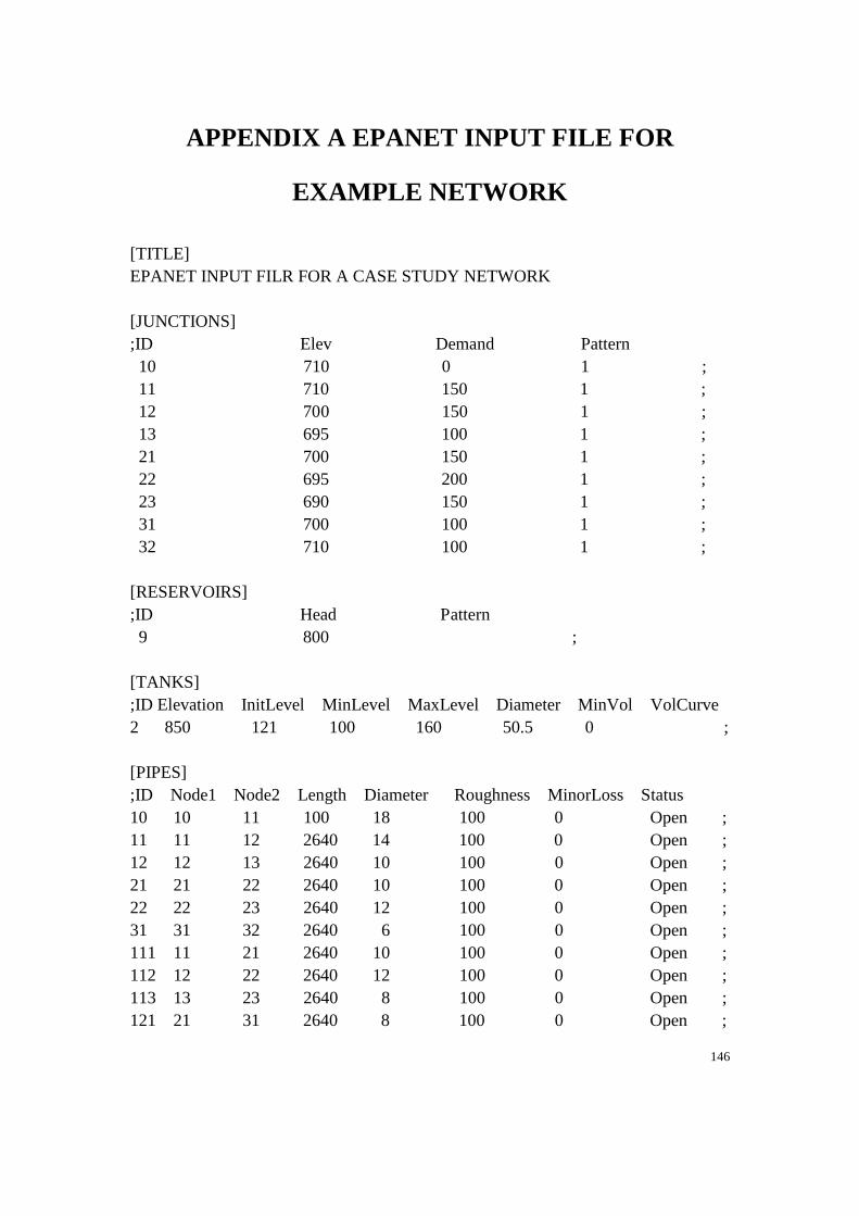
146
APPENDIX A EPANET INPUT FILE FOR
EXAMPLE NETWORK
[TITLE]
EPANET INPUT FILR FOR A CASE STUDY NETWORK
[JUNCTIONS]
;ID Elev Demand Pattern
10 710 0 1 ;
11 710 150 1 ;
12 700 150 1 ;
13 695 100 1 ;
21 700 150 1 ;
22 695 200 1 ;
23 690 150 1 ;
31 700 100 1 ;
32 710 100 1 ;
[RESERVOIRS]
;ID Head Pattern
9 800 ;
[TANKS]
;ID Elevation InitLevel MinLevel MaxLevel Diameter MinVol VolCurve
2 850 121 100 160 50.5 0 ;
[PIPES]
;ID Node1 Node2 Length Diameter Roughness MinorLoss Status
10 10 11 100 18 100 0 Open ;
11 11 12 2640 14 100 0 Open ;
12 12 13 2640 10 100 0 Open ;
21 21 22 2640 10 100 0 Open ;
22 22 23 2640 12 100 0 Open ;
31 31 32 2640 6 100 0 Open ;
111 11 21 2640 10 100 0 Open ;
112 12 22 2640 12 100 0 Open ;
113 13 23 2640 8 100 0 Open ;
121 21 31 2640 8 100 0 Open ;
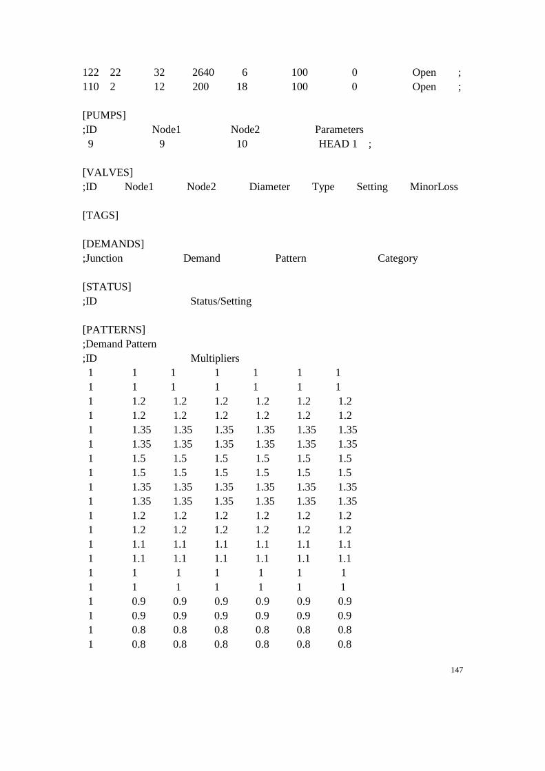
147
122 22 32 2640 6 100 0 Open ;
110 2 12 200 18 100 0 Open ;
[PUMPS]
;ID Node1 Node2 Parameters
9 9 10 HEAD 1 ;
[VALVES]
;ID Node1 Node2 Diameter Type Setting MinorLoss
[TAGS]
[DEMANDS]
;Junction Demand Pattern Category
[STATUS]
;ID Status/Setting
[PATTERNS]
;Demand Pattern
;ID Multipliers
1 1 1 1 1 1 1
1 1 1 1 1 1 1
1 1.2 1.2 1.2 1.2 1.2 1.2
1 1.2 1.2 1.2 1.2 1.2 1.2
1 1.35 1.35 1.35 1.35 1.35 1.35
1 1.35 1.35 1.35 1.35 1.35 1.35
1 1.5 1.5 1.5 1.5 1.5 1.5
1 1.5 1.5 1.5 1.5 1.5 1.5
1 1.35 1.35 1.35 1.35 1.35 1.35
1 1.35 1.35 1.35 1.35 1.35 1.35
1 1.2 1.2 1.2 1.2 1.2 1.2
1 1.2 1.2 1.2 1.2 1.2 1.2
1 1.1 1.1 1.1 1.1 1.1 1.1
1 1.1 1.1 1.1 1.1 1.1 1.1
1 1 1 1 1 1 1
1 1 1 1 1 1 1
1 0.9 0.9 0.9 0.9 0.9 0.9
1 0.9 0.9 0.9 0.9 0.9 0.9
1 0.8 0.8 0.8 0.8 0.8 0.8
1 0.8 0.8 0.8 0.8 0.8 0.8
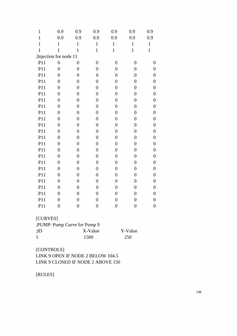
148
1 0.9 0.9 0.9 0.9 0.9 0.9
1 0.9 0.9 0.9 0.9 0.9 0.9
1 1 1 1 1 1 1
1 1 1 1 1 1 1
;Injection for node 11
P11 0 0 0 0 0 0
P11 0 0 0 0 0 0
P11 0 0 0 0 0 0
P11 0 0 0 0 0 0
P11 0 0 0 0 0 0
P11 0 0 0 0 0 0
P11 0 0 0 0 0 0
P11 0 0 0 0 0 0
P11 0 0 0 0 0 0
P11 0 0 0 0 0 0
P11 0 0 0 0 0 0
P11 0 0 0 0 0 0
P11 0 0 0 0 0 0
P11 0 0 0 0 0 0
P11 0 0 0 0 0 0
P11 0 0 0 0 0 0
P11 0 0 0 0 0 0
P11 0 0 0 0 0 0
P11 0 0 0 0 0 0
P11 0 0 0 0 0 0
P11 0 0 0 0 0 0
P11 0 0 0 0 0 0
P11 0 0 0 0 0 0
P11 0 0 0 0 0 0
[CURVES]
;PUMP: Pump Curve for Pump 9
;ID X-Value Y-Value
1 1500 250
[CONTROLS]
LINK 9 OPEN IF NODE 2 BELOW 104.5
LINK 9 CLOSED IF NODE 2 ABOVE 150
[RULES]
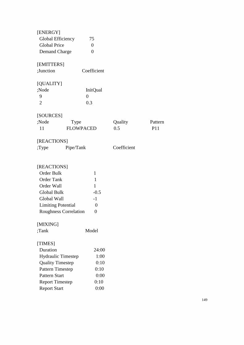
149
[ENERGY]
Global Efficiency 75
Global Price 0
Demand Charge 0
[EMITTERS]
;Junction Coefficient
[QUALITY]
;Node InitQual
9 0
2 0.3
[SOURCES]
;Node Type Quality Pattern
11 FLOWPACED 0.5 P11
[REACTIONS]
;Type Pipe/Tank Coefficient
[REACTIONS]
Order Bulk 1
Order Tank 1
Order Wall 1
Global Bulk -0.5
Global Wall -1
Limiting Potential 0
Roughness Correlation 0
[MIXING]
;Tank Model
[TIMES]
Duration 24:00
Hydraulic Timestep 1:00
Quality Timestep 0:10
Pattern Timestep 0:10
Pattern Start 0:00
Report Timestep 0:10
Report Start 0:00
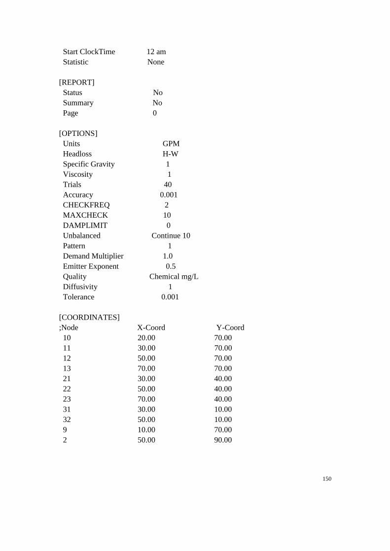
150
Start ClockTime 12 am
Statistic None
[REPORT]
Status No
Summary No
Page 0
[OPTIONS]
Units GPM
Headloss H-W
Specific Gravity 1
Viscosity 1
Trials 40
Accuracy 0.001
CHECKFREQ 2
MAXCHECK 10
DAMPLIMIT 0
Unbalanced Continue 10
Pattern 1
Demand Multiplier 1.0
Emitter Exponent 0.5
Quality Chemical mg/L
Diffusivity 1
Tolerance 0.001
[COORDINATES]
;Node X-Coord Y-Coord
10 20.00 70.00
11 30.00 70.00
12 50.00 70.00
13 70.00 70.00
21 30.00 40.00
22 50.00 40.00
23 70.00 40.00
31 30.00 10.00
32 50.00 10.00
9 10.00 70.00
2 50.00 90.00

151
[VERTICES]
;Link X-Coord Y-Coord
[LABELS]
;X-Coord Y-Coord Label & Anchor Node
[BACKDROP]
DIMENSIONS 7.00 6.00 73.00 94.00
UNITS None
FILE
OFFSET 0.00 0.00
[END]
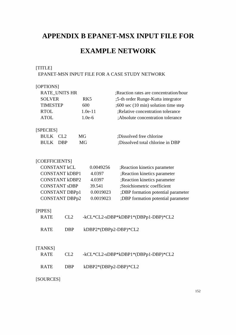
152
APPENDIX B EPANET-MSX INPUT FILE FOR
EXAMPLE NETWORK
[TITLE]
EPANET-MSN INPUT FILE FOR A CASE STUDY NETWORK
[OPTIONS]
RATE_UNITS HR ;Reaction rates are concentration/hour
SOLVER RK5 ;5-th order Runge-Kutta integrator
TIMESTEP 600 ;600 sec (10 min) solution time step
RTOL 1.0e-11 ;Relative concentration tolerance
ATOL 1.0e-6 ;Absolute concentration tolerance
[SPECIES]
BULK CL2 MG ;Dissolved free chlorine
BULK DBP MG ;Dissolved total chlorine in DBP
[COEFFICIENTS]
CONSTANT kCL 0.0049256 ;Reaction kinetics parameter
CONSTANT kDBP1 4.0397 ;Reaction kinetics parameter
CONSTANT kDBP2 4.0397 ;Reaction kinetics parameter
CONSTANT sDBP 39.541 ;Stoichiometric coefficient
CONSTANT DBPp1 0.0019023 ;DBP formation potential parameter
CONSTANT DBPp2 0.0019023 ;DBP formation potential parameter
[PIPES]
RATE CL2 -kCL*CL2-sDBP*kDBP1*(DBPp1-DBP)*CL2
RATE DBP kDBP2*(DBPp2-DBP)*CL2
[TANKS]
RATE CL2 -kCL*CL2-sDBP*kDBP1*(DBPp1-DBP)*CL2
RATE DBP kDBP2*(DBPp2-DBP)*CL2
[SOURCES]
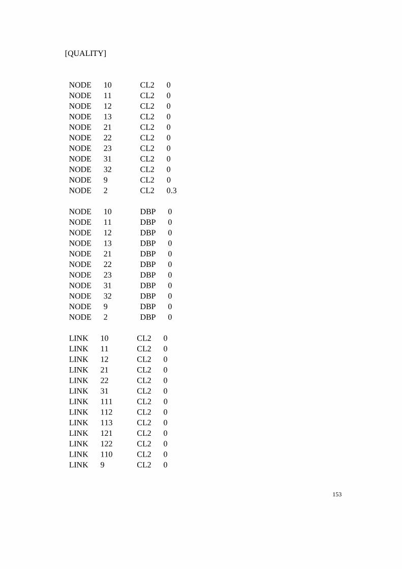
153
[QUALITY]
NODE 10 CL2 0
NODE 11 CL2 0
NODE 12 CL2 0
NODE 13 CL2 0
NODE 21 CL2 0
NODE 22 CL2 0
NODE 23 CL2 0
NODE 31 CL2 0
NODE 32 CL2 0
NODE 9 CL2 0
NODE 2 CL2 0.3
NODE 10 DBP 0
NODE 11 DBP 0
NODE 12 DBP 0
NODE 13 DBP 0
NODE 21 DBP 0
NODE 22 DBP 0
NODE 23 DBP 0
NODE 31 DBP 0
NODE 32 DBP 0
NODE 9 DBP 0
NODE 2 DBP 0
LINK 10 CL2 0
LINK 11 CL2 0
LINK 12 CL2 0
LINK 21 CL2 0
LINK 22 CL2 0
LINK 31 CL2 0
LINK 111 CL2 0
LINK 112 CL2 0
LINK 113 CL2 0
LINK 121 CL2 0
LINK 122 CL2 0
LINK 110 CL2 0
LINK 9 CL2 0
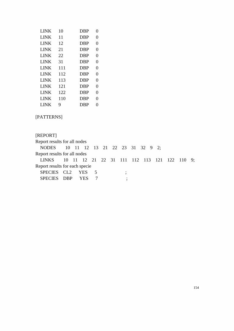
154
LINK 10 DBP 0
LINK 11 DBP 0
LINK 12 DBP 0
LINK 21 DBP 0
LINK 22 DBP 0
LINK 31 DBP 0
LINK 111 DBP 0
LINK 112 DBP 0
LINK 113 DBP 0
LINK 121 DBP 0
LINK 122 DBP 0
LINK 110 DBP 0
LINK 9 DBP 0
[PATTERNS]
[REPORT]
Report results for all nodes
NODES 10 11 12 13 21 22 23 31 32 9 2;
Report results for all nodes
LINKS 10 11 12 21 22 31 111 112 113 121 122 110 9;
Report results for each specie
SPECIES CL2 YES 5 ;
SPECIES DBP YES 7 ;
155
APPENDIX C AN EXAMPLE C-MEX FILE FOR
CALLING EPANET IN MATLAB
#include "mex.h"
#include "epanet2.h"
/*
* an example of C-MEX function that allows to retrieve the
* pressures in all nodes of the network and flows in all pipes.
/*
void ErrorCode(int error)
{
if (error > 100)
{
ENclose();
mexPrintf(" Error code: %d \n",error);
mexErrMsgTxt("There was an error using Epanet");
}
}
/* Main MEX gateway function */
void mexFunction(int nlhs, mxArray *plhs[],int nrhs, const mxArray *prhs[])
{
// Variable declaration
//aux variables to help copy the network name
int fileLen, reportLen, status;
//name of the epanet network file and report file
char *file, *report;
//time of the simulation, hydraulics step
long simTime, hydStep;
//variables for iterational solving of hydraulics
long t, tstep, temp;
//no. of nodes, pipes, tanks
int nNodes, nPipes, nTanks;
int i,j, k;
// variable used to read p(pressure) and f(flow) and q(quality) in nodes and pipes
and source and tank
float pressure,flow,velocity;
// pointers to pressures and flows (output),and quality
156
double *presPtr, *flowPtr;
// checking for the no of inputs
if (nrhs != 2)
mexErrMsgTxt("Two input required");
// Checking if inputs are strings
if( !mxIsChar(prhs[0]) || !mxIsChar(prhs[1]))
mexErrMsgTxt("Input 1 and 2 must be a string.");
//determining the lenght of the file name
fileLen = (mxGetM(prhs[0]) * mxGetN(prhs[0])) + 1;
//memory allocation for the filename
file = mxCalloc(fileLen, sizeof(char));
reportLen = (mxGetM(prhs[1]) * mxGetN(prhs[1])) + 1;
report = mxCalloc(reportLen, sizeof(char));
// Copy sting from prhs[0] to C variable file
status = mxGetString(prhs[0], file, fileLen);
if (status != 0)
mexWarnMsgTxt("Not enough space. String is truncated.");
status = mxGetString(prhs[1], report, reportLen);
if (status != 0)
mexWarnMsgTxt("Not enough space. String is truncated.");
// Opening epanet
ErrorCode(ENopen(file, report, ""));
// Getting the time parameters of the simulation
ErrorCode(ENgettimeparam(EN_DURATION, &simTime));
ErrorCode(ENgettimeparam(EN_HYDSTEP, &hydStep));
// getting the parameters of the network
ErrorCode(ENgetcount(EN_NODECOUNT, &nNodes));
ErrorCode(ENgetcount(EN_TANKCOUNT, &nTanks));
ErrorCode(ENgetcount(EN_LINKCOUNT, &nPipes));
// creating matrices for outputs
plhs[0] = mxCreateDoubleMatrix(nNodes, (simTime / hydStep) + 1,
mxREAL);
plhs[1] = mxCreateDoubleMatrix(nPipes, (simTime / hydStep) + 1,
157
mxREAL);
// assigning the outputs to pointers
presPtr = mxGetPr(plhs[0]);
flowPtr = mxGetPr(plhs[1]);
// initialising the hydraulics epanet solver
ErrorCode(ENopenH());
ErrorCode(ENinitH(1));
j = 0;
temp = 0;
do{
ErrorCode(ENrunH(&t));
// condition for reading the data only on full hydraulics step
if ((temp == hydStep) || (temp == 0))
{
temp = 0;
for( i = 1; i <= nNodes ; i++)
{
ErrorCode(ENgetnodevalue(i, EN_PRESSURE, &pressure));
presPtr[j*(nNodes)+i-1] = pressure;
}
for (k = 1; k <= nPipes; k++)
{
ErrorCode(ENgetlinkvalue(k,EN_FLOW, &flow));
flowPtr[j*nPipes + k-1] = flow;
}
j++;
}
ErrorCode(ENnextH(&tstep));
temp += tstep;
}while( tstep > 0);
ErrorCode(ENcloseH());
ErrorCode(ENclose());
}
158
REFERENCE
[1] M. Brdys and B. Ulanicki, Operational control of water systems: structures,
algorithms and applications: Prentice Hall, 1994.
[2] T. Chang, "Robust model predictive control of water quality in drinking water
distribution systems," University of Birmingham, 2003.
[3] U. S. E. P. Agency, "Drinking Water Priority Rulemaking: Microbial and
Disinfection Byproduct Rules," 2002.
[4] U. EPA, "Basic Information About Drinking Water Disinfection," 2009.
[5] F. Pontius, "Drinking water disinfection with chlorine: an effective public
health practice," Health & Environment Digest, vol. 10, pp. 81-84, 1997.
[6] R. M. Clark and M. Sivaganesan, "Predicting chlorine residuals in drinking
water: Second order model," Journal of water resources planning and
management, vol. 128, pp. 152-161, 2002.
[7] K. Arminski and M. A. Brdys, "Robust monitoring of water quality in drinking
water distribution system," IFAC Proceedings Volumes, vol. 46, pp. 105-110,
2013.
[8] H. Gallard and U. von Gunten, "Chlorination of natural organic matter: kinetics
of chlorination and of THM formation," Water research, vol. 36, pp. 65-74,
2002.
[9] HACH, "Drinking Water Analysis,"
http://uk.hach.com/cms/documents/drinkingwater-downloads/8.%20DW%20o
verview%20brochure%20-%20docID%2010055.pdf.
[10] HACH, "Control of active chlorine disinfection by-products (DBPs) of drinking
water using the THM Plus method. ,"
http://uk.hach.com/cms/documents/drinkingwater-downloads/13.%20Success
%20story%20about%20THM%20measurement%20-%20docID%2020196.pdf
.
[11] K. A. Reynolds. (2007) Vulnerabilities of the Drinking Water Distribution
System. Water Conditioning and Purification.
159
[12] P. F. Boulos, K. E. Lansey, and B. W. Karney, Comprehensive water
distribution systems analysis handbook for engineers and planners: American
Water Works Association, 2006.
[13] M. Xie and M. Brdys, "Nonlinear Model Predictive Control of Water Quality in
Drinking Water Distribution Systems with DBPs Objectives," World Academy
of Science, Engineering and Technology, International Journal of
Mathematical, Computational, Physical, Electrical and Computer Engineering,
vol. 9, pp. 354-360, 2015.
[14] S. E. Hrudey, "Chlorination disinfection by-products, public health risk
tradeoffs and me," Water Research, vol. 43, pp. 2057-2092, 2009.
[15] O. T. Lind and L. Dávalos-Lind, "Interaction of water quantity with water
quality: the Lake Chapala example," Hydrobiologia, vol. 467, pp. 159-167,
2002.
[16] M. Drewa, M. Brdys, and A. Ciminski, "Model predictive control of integrated
quantity and quality in drinking water distribution systems," in Procs. 8th
International IFAC Symposium on Dynamics and Control of Process Systems,
2007.
[17] M. A. Brdys, T. Chang, K. Duzinkiewicz, and W. Chotkowski, "Hierarchical
control of integrated quality and quantity in water distribution systems," in
Procs. ASCE 2000 Joint Conference on Water Resources Engineering and
Water Resources Planning and Management, 2000.
[18] M. Brdys, X. Huang, and Y. Lei, "Two Time-Scale Hierarchical Control of
Integrated Quantity and Quality in Drinking Water Distribution Systems," in
Large scale complex systems theory and applications, 2013, pp. 117-122.
[19] D. Karmeli, Y. Gadish, and S. Meyers, "Design of optimal water distribution
networks," Journal of the Pipeline Division, vol. 94, pp. 1-10, 1968.
[20] S. L. Jacoby, "Design of optimal hydraulic networks," Journal of the
Hydraulics Division, vol. 94, pp. 641-662, 1968.
[21] E. Alperovits and U. Shamir, "Design of optimal water distribution systems,"
Water resources research, vol. 13, pp. 885-900, 1977.
[22] W. Kurek and A. Ostfeld, "Multiobjective water distribution systems control of
pumping cost, water quality, and storage-reliability constraints," Journal of
Water Resources Planning and Management, vol. 140, pp. 184-193, 2012.
160
[23] Y. Dreizin, "Examination of possibilities of energy saving in regional water
supply systems," M. Sc. Thesis, Technion—Israel Institute of Technology,
1970.
[24] M. Sterling and B. Coulbeck, "DYNAMIC-PROGRAMMING SOLUTION
TO OPTIMIZATION OF PUMPING COSTS," vol. 59, ed: THOMAS
TELFORD SERVICES LTD THOMAS TELFORD HOUSE, 1 HERON
QUAY, LONDON, ENGLAND E14 4JD, 1975, pp. 813-818.
[25] A. Diba, P. W. Louie, M. Mahjoub, and W. W. Yeh, "Planned operation of
large-scale water-distribution system," Journal of Water Resources Planning
and Management, vol. 121, pp. 260-269, 1995.
[26] W. Kurek and M. Brdys, "Genetic solver of optimization task of MPC for
optimizing control of integrated quantity and quality in drinking water
distribution systems," in Proc. of the 11th IFAC/IFORS/IMACS/IFIP
Symposium on Large Scale Systems: Theory and Applications, Gdan’sk,
Poland, 2007.
[27] W. Kurek and M. Brdys, "Adaptive multiobjective model predictive control
with application to DWDS," in Large Scale Complex Systems Theory and
Applications, Ecole Centrale de Lille, Villeveneue d'Ascq, France, 2010, pp.
310-315.
[28] D. V. Chase, "A computer program for optimal control of water supply pump
stations: Development and testing," DTIC Document1990.
[29] S. Pezeshk, O. Helweg, and K. Oliver, "Optimal operation of ground-water
supply distribution systems," Journal of Water Resources Planning and
Management, vol. 120, pp. 573-586, 1994.
[30] B. Ulanicki, J. Kahler, and H. See, "Dynamic optimization approach for solving
an optimal scheduling problem in water distribution systems," Journal of Water
Resources Planning and Management, vol. 133, pp. 23-32, 2007.
[31] I. Pulido-Calvo and J. C. Gutiérrez-Estrada, "Selection and operation of
pumping stations of water distribution systems," Environmental Research
Journal, Nova Science Publishers, vol. 5, pp. 1-20, 2011.
[32] D. Broad, G. C. Dandy, and H. R. Maier, "Water distribution system
optimization using metamodels," Journal of Water Resources Planning and
Management, vol. 131, pp. 172-180, 2005.
161
[33] U. Shamir and E. Salomons, "Optimal real-time operation of urban water
distribution systems using reduced models," Journal of Water Resources
Planning and Management, vol. 134, pp. 181-185, 2008.
[34] V. Tran and M. Brdys, "Optimizing control by robustly feasible model
predictive control and application to drinking water distribution systems,"
Artificial Neural Networks–ICANN 2009, pp. 823-834, 2009.
[35] P. H. Gleick, "Water and conflict: Fresh water resources and international
security," International security, vol. 18, pp. 79-112, 1993.
[36] N. W. Arnell, "Climate change and global water resources," Global
environmental change, vol. 9, pp. S31-S49, 1999.
[37] L. A. Rossman, R. M. Clark, and W. M. Grayman, "Modeling chlorine residuals
in drinking-water distribution systems," Journal of environmental engineering,
vol. 120, pp. 803-820, 1994.
[38] M. Brdys and T. Chang, "Robust model predictive control of chlorine residuals
in water systems based on a state space modelling," Water Software Systems:
Theory and Applications, Research Studies Press Ltd., Baldock, Hertfordshire,
England, 2001.
[39] M. Brdys and T. Chang, "Robust model predictive control under output
constraints," in Procs. 15th IFAC World Congress, 2002.
[40] M. Brdys, T. Chang, and K. Duzinkiewicz, "Intelligent model predictive control
of chlorine residuals in water distribution systems," in Proc. 4th ASCE Annual
Water Distribution System Analyse, World Water and Environmental
Resources Congress, 2001.
[41] T. Chang, M. Brdys, and K. Duzinkiewicz, "Decentralised robust model
predictive control of chlorine residuals in drinking water distribution systems,"
in World Water & Environmental Resources Congress 2003, 2004, pp. 1-10.
[42] Z. Wang, M. M. Polycarpou, F. Shang, and J. G. Uber, "Adaptive control
formulation for chlorine residual maintenance in water distribution systems," in
Proc. of the ASCE 2000 Joint Conference on Water Resources Engineering and
Water Resources Planning and Management, 2000.
[43] J. J. Rook, "Formation of haloforms during chlorination of natural waters,"
Water Treat. Exam., vol. 23, pp. 234-243, 1974.
162
[44] T. A. Bellar, J. J. Lichtenberg, and R. C. Kroner, "The occurrence of
organohalides in chlorinated drinking waters," Journal (American Water Works
Association), pp. 703-706, 1974.
[45] P. C. Singer, "Control of disinfection by-products in drinking water," Journal of
environmental engineering, vol. 120, pp. 727-744, 1994.
[46] J. M. Symons, T. A. Bellar, J. K. Carswell, J. DeMarco, K. L. Kropp, G. G.
Robeck, et al., "National organics reconnaissance survey for halogenated
organics," Journal (American Water Works Association), pp. 634-647, 1975.
[47] N. P. Page, Report on carcinogenesis bioassay of chloroform: US Dept. of
Health, Education, and Welfare, Public Health Service, National Institutes of
Health], National Cancer Institute, Division of Cancer Cause and Prevention,
Carcinogenesis Program, Carcinogen Bioassay and Program Resources Branch,
1976.
[48] U. EnvironmentalProtectionAgency, "Nationalinterimprimary drinking water
regulations; control of trihalomethanes in drinking water," Fed. Regist, vol. 44,
pp. 68624-68707, 1979.
[49] B. D. Quimby, M. F. Delaney, P. C. Uden, and R. M. Barnes, "Determination of
the aqueous chlorination products of humic substances by gas chromatography
with microwave plasma emission detection," Analytical Chemistry, vol. 52, pp.
259-263, 1980.
[50] R. F. Christman, D. L. Norwood, D. S. Millington, J. D. Johnson, and A. A.
Stevens, "Identity and yields of major halogenated products of aquatic fulvic
acid chlorination," Environmental science & technology, vol. 17, pp. 625-628,
1983.
[51] J. W. Miller and P. C. Uden, "Characterization of nonvolatile aqueous
chlorination products of humic substances," Environmental science &
technology, vol. 17, pp. 150-157, 1983.
[52] D. A. Reckhow and P. C. Singer, "The removal of organic halide precursors by
preozonation and alum coagulation," Journal (American Water Works
Association), pp. 151-157, 1984.
[53] S. W. Krasner, M. J. McGuire, J. G. Jacangelo, N. L. Patania, K. M. Reagan,
and E. M. Aieta, "The occurrence of disinfection by-products in US drinking
water," Journal-American Water Works Association, vol. 81, pp. 41-53, 1989.
163
[54] N. R. Council, Drinking Water and Health, Volume 7 Disinfectants and
Disinfectant By-Products. Washington, DC: The National Academies Press,
1987.
[55] R. D. Morris, A.-M. Audet, I. F. Angelillo, T. C. Chalmers, and F. Mosteller,
"Chlorination, chlorination by-products, and cancer: a meta-analysis,"
American journal of public health, vol. 82, pp. 955-963, 1992.
[56] M. J. McGuire and R. G. Meadow, "AWWARF trihalomethane survey,"
Journal-American Water Works Association, vol. 80, pp. 61-68, 1988.
[57] D. Water, "National Primary Drinking Water Regulations; Total Coliforms
(including Fecal Coliforms and E. coli)," Final Rule. Fed. Reg, vol. 54, p.
27544.
[58] D. Water, "National Primary Drinking Water Regulations; Filtration,
Disinfection; Turbidity, Giardia lamblia, Viruses, Legionella, and
Heterotrophic Bacteria; Final Rule," Federal Register, June, vol. 28, 1989.
[59] S. Regli, J. Cromwell, X. Zhang, A. Gelderloos, and W. Grubbs, "Framework
for decision making: An EPA perspective," Environmental Protection Agency,
Washington, DC (United States). Office of the Assistant Administrator for
Water1992.
[60] E. G. Means III and S. W. Krasner, "D-DBP regulation: issues and
ramifications," Journal (American Water Works Association), pp. 68-73, 1993.
[61] R. Sadiq and M. J. Rodriguez, "Disinfection by-products (DBPs) in drinking
water and predictive models for their occurrence: a review," Science of the Total
Environment, vol. 321, pp. 21-46, 2004.
[62] M. J. Nieuwenhuijsen, M. B. Toledano, N. E. Eaton, J. Fawell, and P. Elliott,
"Chlorination disinfection byproducts in water and their association with
adverse reproductive outcomes: a review," Occupational and environmental
medicine, vol. 57, pp. 73-85, 2000.
[63] C. Jeong, "Drinking water disinfection by-products: toxicological impacts and
biological mechanisms induced by individual compounds or as complex
mixtures," University of Illinois at Urbana-Champaign, 2014.
[64] S. D. Richardson and C. Postigo, "Drinking water disinfection by-products," in
Emerging organic contaminants and human health, ed: Springer, 2011, pp.
93-137.
164
[65] A. Ostfeld and U. Shamir, "Optimal operation of multiquality networks. I:
Steady-state conditions," Journal of Water Resources Planning and
Management, vol. 119, pp. 645-662, 1993.
[66] A. Ostfeld and U. Shamir, "Optimal operation of multiquality networks. II:
Unsteady conditions," Journal of Water Resources Planning and Management,
vol. 119, pp. 663-684, 1993.
[67] M. Brdys, H. Puta, E. Arnold, K. Chen, and S. Hopfgarten, "Operational control
of integrated quality and quantity in water systems," in Procs..
IFAC/IFORS/IMACS Symposium. on Large Scale Complex Systems: Theory
and Applications, 1995.
[68] A. B. A. Sakarya and L. W. Mays, "Optimal operation of water distribution
pumps considering water quality," Journal of Water Resources Planning and
Management, vol. 126, pp. 210-220, 2000.
[69] K. Duzinkiewicz, M. Brdys, and T. Chang, "Hierarchical model predictive
control of integrated quality and quantity in drinking water distribution
systems," Urban Water Journal, vol. 2, pp. 125-137, 2005.
[70] M. Drewa, M. Brdys, and A. Cimiński, "Model predictive control of integrated
quantity and quality in drinking water distribution systems," IFAC Proceedings
Volumes, vol. 40, pp. 95-100, 2010.
[71] T. D. Prasad, G. Walters, and D. Savic, "Booster disinfection of water supply
networks: Multiobjective approach," Journal of Water Resources Planning and
Management, vol. 130, pp. 367-376, 2004.
[72] D. L. Boccelli, M. E. Tryby, J. G. Uber, L. A. Rossman, M. L. Zierolf, and M.
M. Polycarpou, "Optimal scheduling of booster disinfection in water
distribution systems," Journal of Water Resources Planning and Management,
vol. 124, pp. 99-111, 1998.
[73] M. E. Tryby, D. L. Boccelli, J. G. Uber, and L. A. Rossman, "Facility location
model for booster disinfection of water supply networks," Journal of Water
Resources Planning and Management, vol. 128, pp. 322-333, 2002.
[74] G. Ewald, W. Kurek, and M. A. Brdys, "Grid implementation of a parallel
multiobjective genetic algorithm for optimized allocation of chlorination
stations in drinking water distribution systems: Chojnice case study," IEEE
Transactions on Systems, Man, and Cybernetics, Part C (Applications and
Reviews), vol. 38, pp. 497-509, 2008.
165
[75] G. Ewald, T. Zubowicz, and M. A. Brdys, "Multiprocessor implementation of
Parallel Multiobjective Genetic Algorithm for Optimized Allocation of
Chlorination Stations in Drinking Water Distribution System-a new water
quality model approach," IFAC Proceedings Volumes, vol. 46, pp. 123-128,
2013.
[76] B. H. Lee and R. A. Deininger, "Optimal locations of monitoring stations in
water distribution system," Journal of Environmental Engineering, vol. 118,
pp. 4-16, 1992.
[77] W. E. Hart and R. Murray, "Review of sensor placement strategies for
contamination warning systems in drinking water distribution systems,"
Journal of Water Resources Planning and Management, vol. 136, pp. 611-619,
2010.
[78] J. Berry, W. E. Hart, C. A. Phillips, J. G. Uber, and T. M. Walski, "Water
quality sensor placement in water networks with budget constraints," in Proc.
ASCE/EWRI (Environmental & Water Resources Institute) Conf., Anchorage,
Alaska, 2005.
[79] G. Trachtman, "A Strawman, Common Sense Approach for Water Quality
Sensor Site Selection., 2006, ch. 105," ed.
[80] R. Bahadur, W. B. Samuels, W. Grayman, D. Amstutz, and J. Pickus,
"PipelineNet: A model for monitoring introduced contaminants in a distribution
system," in Proc., World Water & Environmental Resources Congress 2003
and Related Symposia, 2003.
[81] S. R. Ghimire and B. D. Barkdoll, "A heuristic method for water quality sensor
location in a municipal water distribution system: Mass related based
approach," in Proc., 8th Annual Water Distribution System Analysis Symp,
2006.
[82] J. Xu, P. S. Fischbeck, M. J. Small, J. M. VanBriesen, and E. Casman,
"Identifying sets of key nodes for placing sensors in dynamic water distribution
networks," Journal of Water Resources Planning and Management, vol. 134,
pp. 378-385, 2008.
[83] M. A. Brdys, K. Duzinkiewicz, M. Grochowski, and T. Rutkowski, "Robust
estimation of integrated hydraulics and parameters in water distribution
systems," in Bridging the Gap: Meeting the World's Water and Environmental
Resources Challenges, 2001, pp. 1-12.
166
[84] M. Brdys and Y. Kang, "Algorithms for state bounding in large‐ scale
systems," International journal of adaptive control and signal processing, vol.
8, pp. 103-118, 1994.
[85] M. Milanese, J. Norton, H. Piet-Lahanier, and É. Walter, Bounding approaches
to system identification: Springer Science & Business Media, 2013.
[86] M. A. Brdys and K. Chen, "Set membership estimation of state and parameters
in quantity models of water supply and distribution systems,"
at-Automatisierungstechnik, vol. 43, pp. 77-84, 1995.
[87] M. Brdys and K. Chen, "Joint estimation of states and parameters of integrated
quantity and quality models of dynamic water supply and distribution systems,"
in Proc. 13th IFAC World Congress, San Francisco, 1996, pp. 73-78.
[88] H. L. Smith, Monotone dynamical systems: an introduction to the theory of
competitive and cooperative systems: American Mathematical Soc., 2008.
[89] J.-L. Gouzé, A. Rapaport, and M. Z. Hadj-Sadok, "Interval observers for
uncertain biological systems," Ecological modelling, vol. 133, pp. 45-56, 2000.
[90] M. Hadj-Sadok and J. Gouzé, "Estimation of uncertain models of activated
sludge processes with interval observers," Journal of Process Control, vol. 11,
pp. 299-310, 2001.
[91] T. Raïssi, G. Videau, and A. Zolghadri, "Interval observer design for
consistency checks of nonlinear continuous-time systems," Automatica, vol. 46,
pp. 518-527, 2010.
[92] R. Łangowski and M. Brdys, "Monitoring of chlorine concentration in drinking
water distribution systems using an interval estimator," International Journal of
Applied Mathematics and Computer Science, vol. 17, pp. 199-216, 2007.
[93] L. A. Rossman, P. F. Boulos, and T. Altman, "Discrete volume-element method
for network water-quality models," Journal of Water Resources Planning and
Management, vol. 119, pp. 505-517, 1993.
[94] M. M. Polycarpou, J. G. Uber, Z. Wang, F. Shang, and M. Brdys, "Feedback
control of water quality," IEEE Control Systems, vol. 22, pp. 68-87, 2002.
[95] T. Zubowicz, K. Arminski, and M. A. Brdys, "Quality model for integrated
security monitoring and control in water distribution systems," in Intelligent
167
Control and Automation (WCICA), 2012 10th World Congress on, 2012, pp.
3107-3112.
[96] M. Morari and J. H. Lee, "Model predictive control: past, present and future,"
Computers & Chemical Engineering, vol. 23, pp. 667-682, 1999.
[97] J. H. Lee, "Model predictive control: Review of the three decades of
development," International Journal of Control, Automation and Systems, vol.
9, pp. 415-424, 2011.
[98] C. E. Garcia, D. M. Prett, and M. Morari, "Model predictive control: theory and
practice—a survey," Automatica, vol. 25, pp. 335-348, 1989.
[99] J. Richalet, A. Rault, J. Testud, and J. Papon, "Model predictive heuristic
control: Applications to industrial processes," Automatica, vol. 14, pp. 413-428,
1978.
[100] C. R. Cutler and B. L. Ramaker, "Dynamic matrix control-A computer control
algorithm," in joint automatic control conference, San Francisco, CA, 1980, p.
72.
[101] D. W. Clarke, C. Mohtadi, and P. Tuffs, "Generalized predictive control—Part
I. The basic algorithm," Automatica, vol. 23, pp. 137-148, 1987.
[102] D. CLARKF, C. Mohtadi, and P. Tuffs, "Generalized predictive control Part II.
Extensions and interpretations," Automatica, vol. 23, pp. 149-160, 1987.
[103] H. Kwakernaak and R. Sivan, Linear optimal control systems vol. 1:
Wiley-interscience New York, 1972.
[104] E. G. Gilbert and K. T. Tan, "Linear systems with state and control constraints:
The theory and application of maximal output admissible sets," IEEE
Transactions on Automatic control, vol. 36, pp. 1008-1020, 1991.
[105] A. Zheng and M. Morari, "Control of linear unstable systems with constraints,"
in American Control Conference, Proceedings of the 1995, 1995, pp.
3704-3708.
[106] E. Polak and T. Yang, "Moving horizon control of linear systems with input
saturation and plant uncertainty part 1. robustness," International Journal of
Control, vol. 58, pp. 613-638, 1993.
168
[107] E. Polak and T. Yang, "Moving horizon control of linear systems with input
saturation and plant uncertainty part 2. disturbance rejection and tracking,"
International Journal of Control, vol. 58, pp. 639-663, 1993.
[108] S. a. Keerthi and E. G. Gilbert, "Optimal infinite-horizon feedback laws for a
general class of constrained discrete-time systems: Stability and
moving-horizon approximations," Journal of optimization theory and
applications, vol. 57, pp. 265-293, 1988.
[109] V. Nevistić and J. A. Primbs, "Finite receding horizon linear quadratic control:
A unifying theory for stability and performance analysis," 1997.
[110] J. A. Primbs and V. Nevistic, "Constrained finite receding horizon linear
quadratic control," in Decision and Control, 1997., Proceedings of the 36th
IEEE Conference on, 1997, pp. 3196-3201.
[111] W. C. Li and L. T. Biegler, "Process control strategies for constrained nonlinear
systems," Industrial & engineering chemistry research, vol. 27, pp. 1421-1433,
1988.
[112] N. Bhat and T. J. McAvoy, "Use of neural nets for dynamic modeling and
control of chemical process systems," Computers & Chemical Engineering,
vol. 14, pp. 573-582, 1990.
[113] A. A. PATWARDHAN, J. B. RAWLINGS, and T. F. EDGAR, "Nonlinear
model predictive control," Chemical Engineering Communications, vol. 87, pp.
123-141, 1990.
[114] E. Eskinat, S. H. Johnson, and W. L. Luyben, "Use of Hammerstein models in
identification of nonlinear systems," AIChE Journal, vol. 37, pp. 255-268,
1991.
[115] C. E. Hernandez, "Control of nonlinear systems using input-output
information," 1992.
[116] H. J. Tulleken, "Grey-box modelling and identification using physical
knowledge and Bayesian techniques," Automatica, vol. 29, pp. 285-308, 1993.
[117] A. Koulouris, "Multiresolution learning in nonlinear dynamic process modeling
and control," Massachusetts Institute of Technology, 1995.
[118] B. R. Maner, F. J. Doyle, B. A. Ogunnaike, and R. K. Pearson, "Nonlinear
model predictive control of a simulated multivariable polymerization reactor
169
using second-order Volterra models," Automatica, vol. 32, pp. 1285-1301,
1996.
[119] S. Norquay, A. Palazoglu, and J. Romagnoli, "Nonlinear model predictive
control of pH neutralization using Wiener models," in Proceedings of IFAC
World Congress, San Francisco. Time (second) pH, 1996.
[120] D. Q. Mayne and H. Michalska, "Receding horizon control of nonlinear
systems," IEEE Transactions on automatic control, vol. 35, pp. 814-824, 1990.
[121] H. Michalska and D. Q. Mayne, "Robust receding horizon control of
constrained nonlinear systems," IEEE transactions on automatic control, vol.
38, pp. 1623-1633, 1993.
[122] H. Chen and F. Allgöwer, "A quasi-infinite horizon nonlinear model predictive
control scheme with guaranteed stability," in Control Conference (ECC), 1997
European, 1997, pp. 1421-1426.
[123] H. Chen and F. Allgöwer, "A quasi-infinite horizon predictive control scheme
for constrained nonlinear systems," in Proc. 16th Chinese Control Conference,
1996, pp. 309-316.
[124] T. Yang and E. Polak, "Moving horizon control of nonlinear systems with input
saturation, disturbances and plant uncertainty," International Journal of
Control, vol. 58, pp. 875-903, 1993.
[125] S. L. de Oliveira Kothare and M. Morari, "Contractive model predictive control
for constrained nonlinear systems," IEEE Transactions on Automatic Control,
vol. 45, pp. 1053-1071, 2000.
[126] V. Nevistic and M. Morari, "Constrained control of feedback-linearizable
systems," in Proc. 3rd European Control Conference ECC’95, 1995, pp.
1726-1731.
[127] C. Garcia, "Quadratic dynamic matrix control of nonlinear processes: An
application to a batch reaction process," in AIChE annual meeting, 1984.
[128] G. Gattu and E. Zafiriou, "Nonlinear quadratic dynamic matrix control with
state estimation," Industrial & engineering chemistry research, vol. 31, pp.
1096-1104, 1992.
170
[129] J. H. Lee and N. L. Ricker, "Extended Kalman filter based nonlinear model
predictive control," Industrial & Engineering Chemistry Research, vol. 33, pp.
1530-1541, 1994.
[130] S. L. De Oliveira, Model predictive control for constrained nonlinear systems:
vdf Hochschulverlag AG, 1996.
[131] V. Nevistić, "Constrained control of nonlinear systems," Diss. Techn. Wiss.
ETH Zürich, Nr. 12042, 1997. Ref.: M. Morari; Korref.: D. Bonvin, 1997.
[132] A. Zheng, "A computationally efficient nonlinear MPC algorithm," in
American Control Conference, 1997. Proceedings of the 1997, 1997, pp.
1623-1627.
[133] E. Zafiriou, "On the closed-loop stability of constrained QDMC," in American
Control Conference, 1991, 1991, pp. 2367-2372.
[134] J. Lee and Z. Yu, "Tuning of model predictive controllers for robust
performance," Computers & chemical engineering, vol. 18, pp. 15-37, 1994.
[135] J. A. Primbs and V. Nevistic, "A framework for robustness analysis of
constrained finite receding horizon control," IEEE Transactions on Automatic
Control, vol. 45, pp. 1828-1838, 2000.
[136] P. J. Campo and M. Morari, "Robust model predictive control," in American
Control Conference, 1987, 1987, pp. 1021-1026.
[137] Z. Q. Zheng and M. Morari, "Robust stability of constrained model predictive
control," in American Control Conference, 1993, 1993, pp. 379-383.
[138] E. Zafiriou, "Robust model predictive control of processes with hard
constraints," Computers & Chemical Engineering, vol. 14, pp. 359-371, 1990.
[139] H. Genceli and M. Nikolaou, "Robust stability analysis of constrained l1‐
norm model predictive control," AIChE Journal, vol. 39, pp. 1954-1965, 1993.
[140] A. Zheng and M. Morari, "Robust control of linear time-varying systems with
constraints," in Methods of Model Based Process Control, ed: Springer, 1995,
pp. 205-220.
[141] A. Bemporad and M. Morari, "Robust model predictive control: A survey," in
Robustness in identification and control, ed: Springer, 1999, pp. 207-226.
171
[142] Y. J. Wang and J. B. Rawlings, "A new robust model predictive control method
I: theory and computation," Journal of Process Control, vol. 14, pp. 231-247,
2004.
[143] Y. J. Wang and J. B. Rawlings, "A new robust model predictive control method.
II: examples," Journal of Process control, vol. 14, pp. 249-262, 2004.
[144] S. J. Wright, "Applying new optimization algorithms to model predictive
control," in AIChE Symposium Series, 1997, pp. 147-155.
[145] L. Biegler, "Advances in nonlinear programming concepts for process control,"
Journal of Process Control, vol. 8, pp. 301-311, 1998.
[146] F. J. Doyle, J. F. Pekny, P. Dave, and S. Bose, "Specialized programming
methods in the model predictive control of large scale systems," Computers &
chemical engineering, vol. 21, pp. S847-S852, 1997.
[147] M. Kumar, M. Husian, N. Upreti, and D. Gupta, "Genetic algorithm: Review
and application," International Journal of Information Technology and
Knowledge Management, vol. 2, pp. 451-454, 2010.
[148] J. H. Holland, Adaptation in natural and artificial systems: an introductory
analysis with applications to biology, control, and artificial intelligence: U
Michigan Press, 1975.
[149] W. Lee and H.-Y. Kim, "Genetic algorithm implementation in Python," in
Fourth Annual ACIS International Conference on Computer and Information
Science (ICIS'05), 2005, pp. 8-11.
[150] M. Srinivas and L. M. Patnaik, "Genetic algorithms: A survey," Computer, vol.
27, pp. 17-26, 1994.
[151] G. Munavalli and M. M. Kumar, "Optimal scheduling of multiple chlorine
sources in water distribution systems," Journal of water resources planning and
management, vol. 129, pp. 493-504, 2003.
[152] D. Trawicki, K. Duzinkiewicz, and M. Brdys, "Hybrid GA-MIL algorithm for
optimisation of integrated quality and quantity in water distribution systems," in
Procs. World Water & Environmental Resources Congress-EWRI2003, 2003.
[153] B. A. Tolson, H. R. Maier, A. R. Simpson, and B. J. Lence, "Genetic algorithms
for reliability-based optimization of water distribution systems," Journal of
Water Resources Planning and Management, vol. 130, pp. 63-72, 2004.
172
[154] Y. Yamamoto, "An Overview on Repetitive Control---what are the issues and
where does it lead to?," in IFAC Workshop on Periodic Control Systems,
Cernobbio-Como, I, 2001.
[155] W. Findeisen, F. N. Bailey, M. Brdys, K. Malinowski, P. Tatjewski, and A.
Wozniak, "Control and coordination in hierarchical systems," 1980.
[156] K. Chen, "Set membership estimation of state and parameters and operational
control of integrated quantity and quality models of water supply and
distribution systems," PhD Thesis, University of Birmingham, 1997.
[157] B. Coulbeck, "A review of methodologies for modelling and control of water
supply," in Computer applications in water supply: vol. 2---systems
optimization and control, 1988, pp. 80-109.
[158] R. DeMoyer and L. B. Horwitz, A system approach to water distribution
modeling and control: Lexington Books, 1975.
[159] M. L. Zierolf, M. M. Polycarpou, and J. G. Uber, "Development and
autocalibration of an input-output model of chlorine transport in drinking water
distribution systems," IEEE Transactions on Control Systems Technology, vol.
6, pp. 543-553, 1998.
[160] M. Makoudi and L. Radouane, "A robust model reference adaptive control for
non-minimum phase systems with unknown or time-varying delay,"
Automatica, vol. 36, pp. 1057-1065, 2000.
[161] K. Arminski, T. Zubowicz, and M. A. Brdys, "A biochemical multi-species
quality model of a drinking water distribution system for simulation and
design," International Journal of Applied Mathematics and Computer Science,
vol. 23, pp. 571-585, 2013.
[162] R. Łangowski, M. A. Brdys, and R. Qi, "Optimised robust placement of hard
quality sensors for robust monitoring of quality in Drinking Water Distribution
Systems," in Intelligent Control and Automation (WCICA), 2012 10th World
Congress on, 2012, pp. 1109-1114.
[163] A. S. Al-Omari and M. H. Chaudhry, "Unsteady-state inverse chlorine
modeling in pipe networks," Journal of Hydraulic Engineering, vol. 127, pp.
669-677, 2001.
[164] G. Ewald, T. Zubowicz, and M. A. Brdys, "Optimised allocation of actuators
for DWDS," Journal of Process Control, vol. 32, pp. 87-97, 2015.
173
[165] V. N. Tran, "Optimizing model predictive control of processes for wide ranges
of operating conditions," University of Birmingham, 2011.
[166] F. Shang, J. G. Uber, and L. Rossman, "EPANET multi-species extension
user’s manual," Risk Reduction Engineering Laboratory, US Environmental
Protection Agency, Cincinnati, Ohio, 2008.
[167] M. A. Brdys, T. Zubowicz, and K. Arminski, "Robust parameter estimation and
output prediction for reactive carrier-load nonlinear dynamic networks," IFAC
Proceedings Volumes, vol. 46, pp. 426-431, 2013.
[168] J. Kalman, "Continuity and convexity of projections and barycentric
coordinates in convex polyhedra," Pacific Journal of Mathematics, vol. 11, pp.
1017-1022, 1961.