model reduction of large-scale systems - u-bordeaux.fr · model reduction of large-scale systems an...

Model reduction of large-scale systemsAn overview and some recent results

Thanos Antoulas

Rice University

email: [email protected]: www.ece.rice.edu/ aca

POD Workshop, Bordeaux, 31 March - 2 April 2008

Thanos Antoulas ( Rice University ) Model reduction of large-scale systems 1 / 55

Collaborators

• Dan Sorensen, CAAM Rice• Andrew Mayo, ECE Rice• Eduardo Gildin, UT Austin• Mehboob Alam, ECE Rice• Kai Sun, CAAM Rice• Roxana Ionutiu, ECE Rice• Sanda Lefteriu, ECE Rice• Serkan Gugercin, Virginia Tech• Chris Beattie, Virginia Tech• Matthias Heinkenschloss, ECE Rice• Cosmin Ionita, ECE Rice

Contents

1 Introduction and problem statement

2 Motivating Examples

3 Overview of approximation methodsSVD – Krylov – Krylov/SVD

4 Some recent resultsPassivity preserving model reductionOptimal H2 model reductionModel reduction from data

5 Future challenges: Nanoelectronics – References

Contents

Part I

Introduction and model reduction problem

The big picture

��

� discretization

Modeling

Model reduction

��*

Simulation

Controlreduced # of ODEs

ODEs PDEs

��

Physical System and/or Data

The big picture

��

� discretization

Modeling

Model reduction

��*

Simulation

Controlreduced # of ODEs

ODEs PDEs

��

Physical System and/or Data

Dynamical systems

x1(·)x2(·)

...xn(·)

u1(·) −→u2(·) −→

...um(·) −→

−→ y1(·)−→ y2(·)

...−→ yp(·)

We consider explicit state equations

Σ : x(t) = f(x(t), u(t)), y(t) = h(x(t), u(t))

with state x(·) of dimension n � m, p.

Problem statement

Given: dynamical system

Σ = (f, h) with: u(t) ∈ Rm, x(t) ∈ Rn, y(t) ∈ Rp.

Problem: Approximate Σ with:

Σ = (f, h) with : u(t) ∈ Rm, x(t) ∈ Rk , y(t) ∈ Rp, k � n :

(1) Approximation error small - global error bound

(2) Preservation of stability/passivity

(3) Procedure must be computationally efficient

Approximation by projection

Unifying feature of approximation methods: projections.

Let V, W ∈ Rn×k , such that W∗V = Ik ⇒ Π = VW∗ is a projection.Define x = W∗x. Then

{ddt x(t) = W∗f(Vx(t), u(t))

y(t) = h(Vx(t), u(t))

Thus Σ is ”good” approximation of Σ, if x− Πx is ”small”.

Special case: linear dynamical systems

Σ: Ex(t) = Ax(t) + Bu(t), y(t) = Cx(t) + Du(t)

(E, A BC D

)Problem: Approximate Σ by projection: Π = VW∗

(E, A BC D

(W∗EV, W∗AV W∗B

), k � n

Norms:• H∞-norm: worst output error ‖y(t)− y(t)‖ for ‖u(t)‖ = 1.• H2-norm: ‖h(t)− h(t)‖E, An

⇒ E, Ak

Σ: : Σ

(E, A BC D

), k � n

⇒ E, Ak

Σ: : Σ

(E, A BC D

), k � n

⇒ E, Ak

Σ: : Σ

(E, A BC D

), k � n

⇒ E, Ak

Σ: : Σ

Part II

Motivating examples

Motivating Examples: Simulation/Control

1. Passive devices • VLSI circuits• Thermal issues• Power delivery networks

2. Data assimilation • North sea forecast• Air quality forecast

3. Molecular systems • MD simulations• Heat capacity

4. CVD reactor • Bifurcations5. Mechanical systems: •Windscreen vibrations

• Buildings6. Optimal cooling • Steel profile7. MEMS: Micro Electro-

-Mechanical Systems • Elf sensor8. Nano-Electronics • Plasmonics

Passive devices: VLSI circuits

1960’s: IC 1971: Intel 4004 2001: Intel Pentium IV10µ details 0.18µ details2300 components 42M components64KHz speed 2GHz speed

2km interconnect7 layers

Typical GateDelay

1.01.3 0.8 0.30.5Technology (μm)

0.1 0.08

Average WiringDelay

≈ 0.25 μm

Today’s Technology: 65 nm

65nm technology: gate delay < interconnect delay!

Conclusion: Simulations are required to verify that internal electromagneticfields do not significantly delay or distort circuit signals. Thereforeinterconnections must be modeled.

⇒ Electromagnetic modeling of packages and interconnects ⇒ resultingmodels very complex: using PEEC methods (discretization of Maxwell’sequations): n ≈ 105 · · · 106 ⇒ SPICE: inadequate

• Source: van der Meijs (Delft)

Typical GateDelay

1.01.3 0.8 0.30.5Technology (μm)

0.1 0.08

Average WiringDelay

≈ 0.25 μm

Today’s Technology: 65 nm

65nm technology: gate delay < interconnect delay!

Conclusion: Simulations are required to verify that internal electromagneticfields do not significantly delay or distort circuit signals. Thereforeinterconnections must be modeled.

⇒ Electromagnetic modeling of packages and interconnects ⇒ resultingmodels very complex: using PEEC methods (discretization of Maxwell’sequations): n ≈ 105 · · · 106 ⇒ SPICE: inadequate

• Source: van der Meijs (Delft)

Power delivery network for VLSI chips

r r r rr r r r

r r r rr r r r�

��

AA AA AA AA

#states ≈ 8 · 106

#inputs/outputs ≈ 1 · 106

Mechanical systems: cars

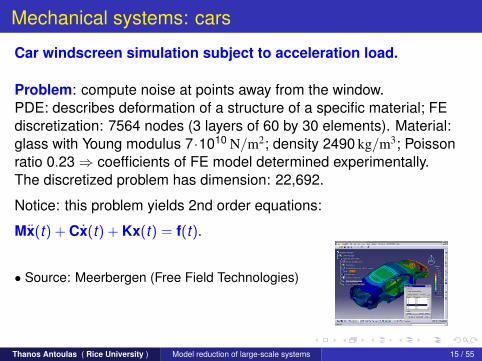
Car windscreen simulation subject to acceleration load.

Problem: compute noise at points away from the window.PDE: describes deformation of a structure of a specific material; FEdiscretization: 7564 nodes (3 layers of 60 by 30 elements). Material:glass with Young modulus 7·1010 N/m2; density 2490 kg/m3; Poissonratio 0.23 ⇒ coefficients of FE model determined experimentally.The discretized problem has dimension: 22,692.

Notice: this problem yields 2nd order equations:

Mx(t) + Cx(t) + Kx(t) = f(t).

• Source: Meerbergen (Free Field Technologies)

Mechanical Systems: BuildingsEarthquake prevention

Taipei 101: 508m Damper between 87-91 floors 730 ton damper

Building Height Control mechanism Damping frequencyDamping mass

CN Tower, Toronto 533 m Passive tuned mass damperHancock building, Boston 244 m Two passive tuned dampers 0.14Hz, 2x300tSydney tower 305 m Passive tuned pendulum 0.1,0.5z, 220tRokko Island P&G, Kobe 117 m Passive tuned pendulum 0.33-0.62Hz, 270tYokohama Landmark tower 296 m Active tuned mass dampers (2) 0.185Hz, 340tShinjuku Park Tower 296 m Active tuned mass dampers (3) 330tTYG Building, Atsugi 159 m Tuned liquid dampers (720) 0.53Hz, 18.2t

• Source: S. WilliamsThanos Antoulas ( Rice University ) Model reduction of large-scale systems 16 / 55

MEMS: Elk sensor

Mercedes A Class semiconductor rotation sensor

• Source: Laur (Bremen)

Part III

Overview of approximation methods

Approximation methods: OverviewPPPPPPPPq

��

Krylov

• Realization• Interpolation• Lanczos• Arnoldi

��

Nonlinear systems Linear systems• POD methods • Balanced truncation• Empirical Gramians • Hankel approximation

��

Krylov/SVD Methods

��

Krylov

��

Krylov/SVD Methods

��

Krylov

��

Krylov/SVD Methods

��

Krylov

��

Krylov/SVD Methods

SVD Approximation methodsA prototype approximation problem – the SVD

(Singular Value Decomposition): A = UΣV∗.

Supernova Clown

0.5 1 1.5 2 2.5

Singular values of Clown and Supernova Supernova: original picture

Supernova: rank 6 approximation Supernova: rank 20 approximation

green: clownred: supernova(log−log scale)

Clown: original picture Clown: rank 6 approximation

Clown: rank 12 approximation Clown: rank 20 approximation

Singular values provide trade-off between accuracy and complexity

SVD Approximation methodsA prototype approximation problem – the SVD

(Singular Value Decomposition): A = UΣV∗.

Supernova Clown

0.5 1 1.5 2 2.5

Singular values of Clown and Supernova Supernova: original picture

Supernova: rank 6 approximation Supernova: rank 20 approximation

green: clownred: supernova(log−log scale)

Clown: original picture Clown: rank 6 approximation

Clown: rank 12 approximation Clown: rank 20 approximation

Singular values provide trade-off between accuracy and complexity

POD: Proper Orthogonal Decomposition

Consider: x(t) = f(x(t), u(t)), y(t) = h(x(t), u(t)).Snapshots of the state:

X = [x(t1) x(t2) · · · x(tN)] ∈ Rn×N

SVD: X = UΣV∗ ≈ UkΣk V∗k , k � n. Approximate the state:

x(t) = U∗k x(t) ⇒ x(t) ≈ Uk x(t), x(t) ∈ Rk

Project state and output equations. Reduced order system:

˙x(t) = U∗k f(Uk x(t), u(t)), y(t) = h(Uk x(t), u(t))

⇒ x(t) evolves in a low-dimensional space.

Issues with POD:(a) Choice of snapshots, (b) singular values not I/O invariants.

X = [x(t1) x(t2) · · · x(tN)] ∈ Rn×N

SVD methods: balanced truncation

Trade-off between accuracy and complexity for linear dynamical systems isprovided by the Hankel Singular Values. Define the gramians as solutionsof the Lyapunov equations

AP + PA∗ + BB∗ = 0, P > 0A∗Q + QA + C∗C = 0, Q > 0

}⇒ σi =

√λi(PQ)

σi : Hankel singular values of the system. There exists balanced basiswhere P = Q = S = diag (σ1, · · · , σn). In this basis partition:

(A11 A12

A21 A22

), B =

), C = (C1 | C2), S =

(Σ1 00 Σ2

The reduced system is obtained by balanced truncation(A11 B1

), where Σ2 contains the small Hankel singular values.

Properties of balanced reduction

1 Stability is preserved2 Global error bound:

σk+1 ≤‖ Σ− Σ ‖∞≤ 2(σk+1 + · · ·+ σn)

Drawbacks

1 Dense computations, matrix factorizations and inversions ⇒ maybe ill-conditioned

2 Need whole transformed system in order to truncate ⇒ number ofoperations O(n3)

3 Bottleneck: solution of two Lyapunov equations

Properties of balanced reduction

1 Stability is preserved2 Global error bound:

σk+1 ≤‖ Σ− Σ ‖∞≤ 2(σk+1 + · · ·+ σn)

Drawbacks

1 Dense computations, matrix factorizations and inversions ⇒ maybe ill-conditioned

2 Need whole transformed system in order to truncate ⇒ number ofoperations O(n3)

3 Bottleneck: solution of two Lyapunov equations

Approximation methods: Krylov methodsPPPPPPPPq

��

Krylov

��

Krylov/SVD Methods

Approximation methods: Krylov methodsPPPPPPPPq

��

Krylov

��

Krylov/SVD Methods

The basic Krylov iteration

Given A ∈ Rn×n and b ∈ Rn, let v1 = b‖b‖ . At the k th step:

AVk = Vk Hk + fk e∗k where

ek ∈ Rk : canonical unit vectorVk = [v1 · · · vk ] ∈ Rk×k , V∗v Vk = IkHk = V∗k AVk ∈ Rk×k

⇒ vk+1 = fk‖fk‖ ∈ Rn

Computational complexity for k steps: O(n2k); storage O(nk).

The Lanczos and the Arnoldi algorithms result.

The Krylov iteration involves the subspace Rk =[b, Ab, · · · , Ak−1b

• Arnoldi iteration ⇒ arbitrary A ⇒ Hk upper Hessenberg.• Symmetric (one-sided) Lanczos iteration ⇒ symmetric A = A∗

⇒ Hk tridiagonal and symmetric.• Two-sided Lanczos iteration with two starting vectors b, c

⇒ arbitrary A ⇒ Hk tridiagonal.

Three uses of the Krylov iteration

(1) Iterative solution of Ax = b: approximate the solution x iteratively.

(2) Iterative approximation of the eigenvalues of A. In this case b is not fixedapriori. The eigenvalues of the projected Hk approximate the dominanteigenvalues of A.

(3) Approximation of linear systems by moment matriching.

⇒ Item (3) is of interest in the present context.

Approximation by moment matching

Given Ex(t) = Ax(t) + Bu(t), y(t) = Cx(t) + Du(t), expand transfer functionaround s0: