model selection, criticism, and averaging - statistical...

Model selection, criticism, and averaging

Rebecca C. Steorts

October 18, 2015

Model criticism

I There is more to statistical inference than just obtainingestimates and predictions

I One art of inference is in model choiceI Once we have settled on a few models or families of models,

there are some tools that can help us perform model selection

Using posterior predictive

I Use the posterior predictive distributionI We can obtain sample datasets from the posterior predictive

and compare aspects of these calculated from the “true” dataI Usually we are checking to see whether the “true” data would

be an unlikely realization from the predictive distribution

Prior sensitivity

I We can also look at the prior sensitivityI If the prior parameterization effects the posterior inference

significantly, then this leads to inference that is not robustI Can test robustness of the prior sensitivity analysisI Test how stable statistics are that you’re interested in regarding

the choice of the priorI These are called prior predictive checks

Model comparison

I Posterior predictive checks, and prior sensitivity analysesrepresent a special type of model criticism that is absolute

I “All models are wrong [and thus easily criticized], but some areuseful” (Box and Draper, 1987, pp. 424)

I This suggests that comparing models to one another, ratherthan criticizing them in a vacuum, may be more useful

I We prefere a criticism that is relative

Starting simple

I There are many options in setting up a model for an appliedproblem

I It is sensible to start with a simple model that is easy to workwith, but may only use some of the available information, e.g.,

I not using some explanatory variables in a regressionI fitting a normal model to discrete dataI ignoring evidence of unequal variances

Model expansion

I Once we have a simple model, when should we make it morecomplex?

I How should we compare models?

Posterior Odds Ratio

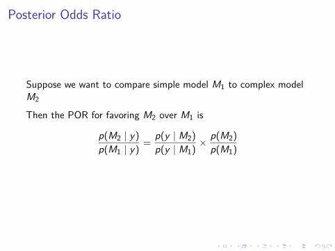
Suppose we want to compare simple model M1 to complex modelM2

Then the POR for favoring M2 over M1 is

p(M2 | y)p(M1 | y) = p(y | M2)

p(y | M1) ×p(M2)p(M1)

Calculating BFs

I Often POR = BF when the prior for the models is equalp(M2)/p(M1) = 1 or rather equal prior odds

I BFs/PORs are very general methods for comparing models, butthey can be difficult to compute due to the integrals involved

I Many specialized MC techniques have recently been developedto help approximate BFs

I There are some important special cases where the integrals areanalytically tractable

Example: Bayesian Linear Models

I Suppose we have a linear model and two models to compare

M2 : Y = Np2(X2β, σ2Ip2)

M1 : Y = Np1(X1β, σ2Ip1)

where X1,X2 are two different design matrices with p2, p1columns respectively.

I For example, X2 may contain quadratic terms but X1 may not.

Example: Key integral(s)

I The important integral(s) for calculating the BF for comparingtwo linear models are like:

p(y | X ) =∫

p(y , σ2 | X ) dσ2 =∫

p(y | X , σ2)p(σ2) dσ2

p(σ2 | X , y) = c1 × p(y | X , σ2)p(σ2) = c1c2 × IG(σ2, an/2, bn/2)

where an, bn depend on prior p(β, σ2)

Example: Closed form BF

Since the IG density integrates to 1, we have that

p(y | X ) = 1/(c1c2)

If we use “Jeffrey’s prior“, it’s possilbe to find c1(X ) and c2(X ) inclosed form. (It does involve some algebra and math).

Interpretating BFs

Jeffrey’s gave a scale for interpreting the BF

Bayes Factor Strength of evidence

< 1:1 Negative1:1 to 3:1 Barely worth mentioning3:1 to 10:1 Substantial10:1 to 30:1 Strong30:1 to 100:1 Very strong> 100:1 Decisive

The spirit is different than a classical hypothesis test Bayesiansdon’t “accept” or “fail to reject”, but rather focus on the evidencein relative probabilities

Recall classical model selction

I Forward and backward selectionI AIC and BIC

Bayesian model selection

I There are many variants on this.I We will focus on just one, which is widely used and works well

in practice.I Bayesian model averaging: fully Bayesian approach.I Simple idea is average over all posterior predictions

p(y | y) =∫

p(y | M, y)dM

≈ 1/S∑

p(y | M(s), y)

= 1/S∑

p(y | X (s), y)

More on Bayesian model averaging

I The same applied to other functions/quantities common to allmodels.

π(θ | y) =∑

π(θ | y ,Mi)π(Mi | y)

where θ is common to all models M, e.g., σ2 in regressionsI The model-averaged approach provides a single parameter

estimate based on all plausible models Mi by weighting eachaccording to π(Mi | y)

I Such estimates are said to take model uncertainty into account

Example of Diabetes data

I Ten baseline measures: age, sex, BMI, average BP, etcI 442 diabetes patientsI Response variable: measure of diasease progression one year

after baselineI Reference: Efron, Hastie, Johnstone, and Tibshirani (2004)

Snapshot of Diabetes data

Loading the data

# load necessary libraries & data #library(monomvn)data(diabetes)attach(diabetes, warn.conflicts=FALSE)#x contains the regression coefficients-it has been##pre-standardized to have a unit L2 norm#

Form the design matrix

#form the full design matrix of##covariates with main effects##quadratic terms and interactions#X <- cbind(x, x[,c(1, 3:10)]^2)cnames <- colnames(x)colnames(X)[11:19] <- paste(cnames[-2], "2", sep="")nc <- 19for(j in 1:(ncol(x)-1)) {for(k in (j+1):ncol(x)) {nc <- nc+1X <- cbind(X, x[,j]*x[,k])colnames(X)[nc] <- paste(cnames[j],cnames[k], sep=".")

}}

Fit the biggest possible model

#start with the biggest possible model#fit <- lm(y~., data=as.data.frame(X))

Summary of this modelEstimate Std. Error t value Pr(>|t|)

(Intercept) 124.928 262.280 0.476 0.634age 50.721 65.513 0.774 0.439sex -267.344 65.270 -4.096 0.000bmi 460.721 84.601 5.446 0.000map 342.933 72.447 4.734 0.000

tc -3599.542 60575.187 -0.059 0.953ldl 3028.281 53238.699 0.057 0.955

hdl 1103.047 22636.179 0.049 0.961tch 74.937 275.807 0.272 0.786ltg 1828.210 19914.504 0.092 0.927glu 62.754 70.398 0.891 0.373

age2 1237.357 1269.870 0.974 0.330bmi2 668.278 1213.988 0.550 0.582map2 -147.209 1246.833 -0.118 0.906

tc2 94161.841 99678.864 0.945 0.345ldl2 46890.019 69698.854 0.673 0.502

hdl2 21173.675 19446.748 1.089 0.277tch2 10439.247 8193.027 1.274 0.203ltg2 22415.265 26716.192 0.839 0.402glu2 1610.410 1327.881 1.213 0.226

age.sex 3179.892 1570.017 2.025 0.044age.bmi -379.402 1673.404 -0.227 0.821age.map 416.330 1714.033 0.243 0.808

age.tc -3255.358 12643.317 -0.257 0.797age.ldl -1412.454 10381.198 -0.136 0.892

age.hdl 4871.293 6532.770 0.746 0.456age.tch 4001.359 4550.207 0.879 0.380age.ltg 2627.608 4716.296 0.557 0.578age.glu 1398.720 1796.626 0.779 0.437sex.bmi 1370.750 1652.686 0.829 0.407sex.map 1929.305 1629.937 1.184 0.237

sex.tc 9073.774 12361.593 0.734 0.463sex.ldl -7457.966 9912.682 -0.752 0.452

sex.hdl -2863.313 6286.918 -0.455 0.649sex.tch -2905.798 4422.459 -0.657 0.512sex.ltg -2527.572 4810.943 -0.525 0.600sex.glu 984.942 1585.331 0.621 0.535

bmi.map 3061.795 1708.606 1.792 0.074bmi.tc -6577.160 14544.473 -0.452 0.651bmi.ldl 5318.768 12353.931 0.431 0.667

bmi.hdl 2729.347 7383.565 0.370 0.712bmi.tch -733.318 5061.331 -0.145 0.885bmi.ltg 2528.662 5644.761 0.448 0.654bmi.glu 487.345 1897.827 0.257 0.797map.tc 10324.628 14727.300 0.701 0.484map.ldl -7120.803 12516.372 -0.569 0.570

map.hdl -3852.867 6368.271 -0.605 0.546map.tch -1259.991 4292.647 -0.294 0.769map.ltg -3469.729 6096.103 -0.569 0.570map.glu -2710.809 1854.529 -1.462 0.145

tc.ldl -130896.297 165433.349 -0.791 0.429tc.hdl -86857.848 84307.507 -1.030 0.304tc.tch -38289.516 30581.549 -1.252 0.211tc.ltg -79664.184 275912.621 -0.289 0.773tc.glu -3906.482 13194.672 -0.296 0.767ldl.hdl 57231.650 68564.324 0.835 0.404ldl.tch 18962.634 23105.969 0.821 0.412ldl.ltg 61076.149 241341.343 0.253 0.800ldl.glu 1835.547 10827.737 0.170 0.865

hdl.tch 22320.367 18823.885 1.186 0.236hdl.ltg 33164.570 104153.881 0.318 0.750hdl.glu 4892.460 6673.848 0.733 0.464tch.ltg 7581.398 12149.373 0.624 0.533tch.glu 4633.734 4621.369 1.003 0.317ltg.glu 1655.114 5245.779 0.316 0.753

Model selection with just main effects

n <- nrow(X)#just main effects#fit2 <- lm(y~., data=as.data.frame(X[,1:10]))print(xtable(summary(fit2)$coef, digits = 3),size='\\tiny', comment = FALSE)

Estimate Std. Error t value Pr(>|t|)(Intercept) 152.133 2.576 59.061 0.000

age -10.012 59.749 -0.168 0.867sex -239.819 61.222 -3.917 0.000bmi 519.840 66.534 7.813 0.000map 324.390 65.422 4.958 0.000

tc -792.184 416.684 -1.901 0.058ldl 476.746 339.035 1.406 0.160

hdl 101.045 212.533 0.475 0.635tch 177.064 161.476 1.097 0.273ltg 751.279 171.902 4.370 0.000glu 67.625 65.984 1.025 0.306

Model selection with main effects and sq. terms#main effects and squared terms#fit3 <- lm(y~., data=as.data.frame(X[,1:19]))print(xtable(summary(fit3)$coef, digits = 3),size='\\tiny',comment = FALSE)


age 41.884 61.220 0.684 0.494sex -242.389 61.387 -3.949 0.000bmi 454.348 74.705 6.082 0.000map 328.310 66.519 4.936 0.000

tc -4802.427 1535.710 -3.127 0.002ldl 4040.048 1342.369 3.010 0.003

hdl 1573.622 609.074 2.584 0.010tch 125.228 256.206 0.489 0.625ltg 2189.001 556.257 3.935 0.000glu 58.268 65.961 0.883 0.378

age2 2343.228 1007.626 2.325 0.021bmi2 1529.486 919.176 1.664 0.097map2 542.101 986.040 0.550 0.583

tc2 1507.216 1620.014 0.930 0.353ldl2 -1681.742 1625.902 -1.034 0.302

hdl2 176.148 1014.390 0.174 0.862tch2 303.683 1258.515 0.241 0.809ltg2 8636.562 3446.492 2.506 0.013glu2 2004.058 782.419 2.561 0.011

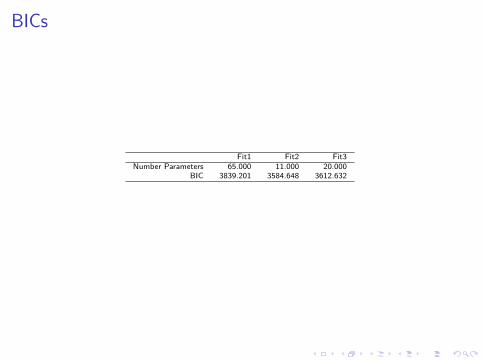
BICs

Fit1 Fit2 Fit3Number Parameters 65.000 11.000 20.000

BIC 3839.201 3584.648 3612.632

Stepwise (both directions)#use step (via BIC)#fit.step <- step(fit,scope=list(upper=~.,lower=~1),k=log(nrow(X)),direction="both",trace=FALSE);bics<-cbind(bics,extractAIC(fit.step,k=log(n)));names(bics)[4]<-'FitStep'print(xtable(summary(fit.step)$coef,digits = 3), size='\\tiny',comment = FALSE)


sex -243.263 58.393 -4.166 0.000bmi 498.454 64.373 7.743 0.000map 323.507 61.226 5.284 0.000

tc -720.079 171.181 -4.207 0.000ldl 529.116 160.846 3.290 0.001ltg 929.017 87.761 10.586 0.000

ltg2 7683.647 2650.725 2.899 0.004glu2 1879.022 761.878 2.466 0.014

age.sex 4536.187 1142.838 3.969 0.000bmi.map 2786.852 1081.865 2.576 0.010

tc.ltg -15296.288 5360.237 -2.854 0.005ldl.ltg 13545.468 4412.505 3.070 0.002

hdl.ltg 6095.024 2315.547 2.632 0.009

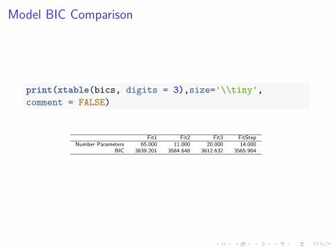
Model BIC Comparison

print(xtable(bics, digits = 3),size='\\tiny',comment = FALSE)

Fit1 Fit2 Fit3 FitStepNumber Parameters 65.000 11.000 20.000 14.000

BIC 3839.201 3584.648 3612.632 3565.904

Let’s go full Bayes#fit the model using a "ridge" prior for stability##see the park and casella paper for details#bfit <- bridge(X,y,T=5000,mprior=c(0.5,0.5),verb=0)#plot the posterior regression coefficients#plot(bfit, burnin=1000);plot(bfit, xlim=c(1,11),ylim=c(-700,800), burnin=1000);plot(bfit,"m")

mu b.3 b.6 b.9 b.13 b.17 b.21 b.25 b.29 b.33 b.37 b.41 b.45 b.49 b.53 b.57 b.61

−10

000

−50

000

5000

1000

0

Boxplots of regression coefficients

coef

mu b.1 b.2 b.3 b.4 b.5 b.6 b.7 b.8 b.9 b.10

−50

00

500

Boxplots of regression coefficients

coef

Histogram of x$m[burnin:x$T]

x$m[burnin:x$T]

Fre

quen

cy

0 10 20 30 40

050

015

00

0 1000 2000 3000 4000 5000

010

2030

40

m chain

burnin:x$T

x$m

[bur

nin:

x$T

]

Summary info#extract the summary#s<-summary(bfit);names(s$bn0)<-colnames(X)r<-sort(s$bn0,decreasing=TRUE)[1:length(coef(fit.step))]#Gives the estimated posterior#probability of coeff begin non zero#print(xtable(as.matrix(r),digits=3),size='\\tiny',comment=FALSE)

xbmi 1.000map 1.000

ltg 1.000sex 0.993

age.sex 0.935hdl 0.898

bmi.map 0.797glu2 0.594

tc.tch 0.584ldl.ltg 0.559

tch 0.499tch.ltg 0.462age.ltg 0.455

tc 0.451

Extract the MAP

m <- which.max(bfit$lpost)bmap <- bfit$beta[m,]names(bmap) <- colnames(X)print(xtable(as.matrix(bmap[bmap>0]),digits=3),size='\\tiny',comment=FALSE)

xbmi 462.986map 267.259

tc 4.529ltg 593.536

age.sex 6279.898age.hdl 1851.345

bmi.map 3013.300map.tc 2427.381

tc.glu 1740.000ldl.ltg 113.247

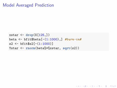
Model Averaged Prediction

xstar <- drop(X[125,])beta <- bfit$beta[-(1:1000),] #burn-in#s2 <- bfit$s2[-(1:1000)]Ystar <- rnorm(beta%*%xstar, sqrt(s2))

Plot of Model Average Predictionhist(Ystar,col='magenta',xlab='Predictions',main='Prediction Distribution')

Prediction Distribution

Predictions

Fre

quen

cy

50 55 60

020

040

060

0

model selection, criticism, and averaging - statistical...

Documents