modeling a loudspeaker as a exible spherical cap on a ... · modeling a loudspeaker as a exible...

Modeling a loudspeaker as a flexible spherical cap on a rigid sphere

Ronald M. Aartsa) and Augustus J.E.M. Janssenb)

Philips Research EuropeHTC 36 (WO-02)NL-5656AE EindhovenThe Netherlands

(Dated: January 26, 2010)

It has been argued that the sound radiation of a loudspeaker is modeled realistically by assuming theloudspeaker cabinet to be a rigid sphere with a moving rigid spherical cap. Series expansions, validin the whole space on and outside the sphere, for the pressure due to a harmonically excited, flexiblecap with an axially symmetric velocity distribution are presented. The velocity profile is expanded infunctions orthogonal on the cap rather than on the whole sphere. This has the advantage that onlya few expansion coefficients are sufficient to accurately describe the velocity profile. An adaptationof the standard solution of the Helmholtz equation to this particular parametrization is required.This is achieved by using recent results on argument scaling in orthogonal Zernike polynomials. Theefficacy of the approach is exemplified by calculating various acoustical quantities with particularattention to certain velocity profiles that vanish at the rim of the cap to a desired degree. Thesequantities are: the sound pressure, polar response, baffle-step response, sound power, directivity,and acoustic center of the radiator. The associated inverse problem, in which the velocity profileis estimated from pressure measurements around the sphere, is feasible as well since the number ofexpansion coefficients to be estimated is limited. This is demonstrated with a simulation.

PACS numbers: 43.38 Ar, 43.20 Bi, 43.20 Px, 43.40 AtKeywords: loudspeaker, loudspeaker characterization, Helmholtz equation with spherical boundaryconditions, flexible pole cap sound radiation, Legendre polynomial, Zernike expansion, scaling Zernikepolynomials

I. INTRODUCTION

The sound radiation of a loudspeaker is commonlymodeled by assuming the loudspeaker cabinet to be arigid infinite baffle around a circularly symmetric mem-brane. Given a velocity distribution on the membrane,the pressure in front of the baffle due to a harmonic ex-citation is then described by the Rayleigh integral1 orby King’s integral2. These integrals have given rise toan impressive arsenal of analytic results and numericalmethods to determine the pressure and other acousti-cal quantities in journal papers3–21 and textbooks22–28.The results thus obtained are in good correspondencewith what one finds, numerically or otherwise, when theloudspeaker is modeled as being a finite-extent box-likecabinet with a circular, vibrating membrane. Here oneshould, however, limit attention to the region in front ofthe loudspeaker and not too far from the axis throughthe middle of and perpendicular to the membrane. Thevalidity of the infinite-baffle model becomes questionable,or even nonsensical, on the side region or behind the loud-speaker26 (p. 181). An alternative model, with potentialfor more adequately dealing with the latter regions, as-sumes the loudspeaker to be a rigid sphere equipped witha membrane in a spherical cap of the sphere.

a)[email protected]; Also at Technical UniversityEindhoven, Den Dolech 2, PT3.23, P.O Box 513, NL-5600 MBEindhoven, The Netherlandsb)[email protected]

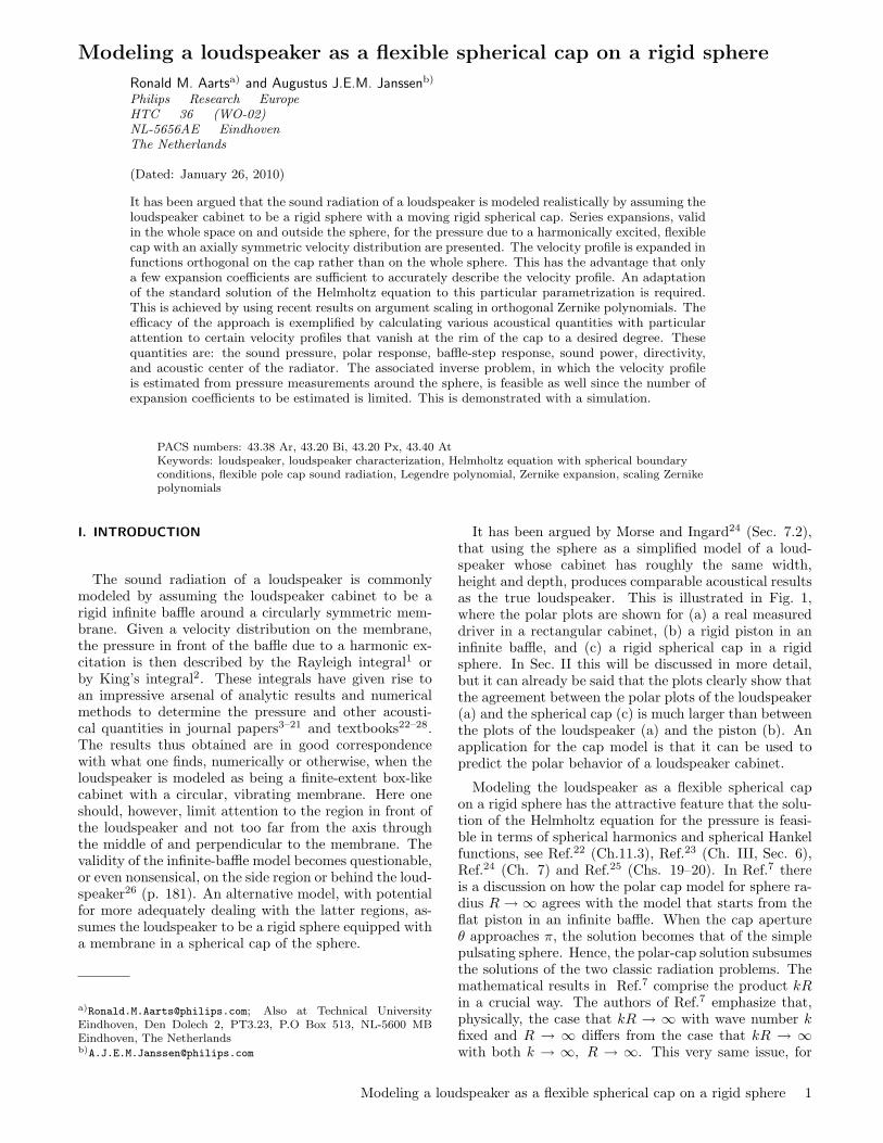
It has been argued by Morse and Ingard24 (Sec. 7.2),that using the sphere as a simplified model of a loud-speaker whose cabinet has roughly the same width,height and depth, produces comparable acoustical resultsas the true loudspeaker. This is illustrated in Fig. 1,where the polar plots are shown for (a) a real measureddriver in a rectangular cabinet, (b) a rigid piston in aninfinite baffle, and (c) a rigid spherical cap in a rigidsphere. In Sec. II this will be discussed in more detail,but it can already be said that the plots clearly show thatthe agreement between the polar plots of the loudspeaker(a) and the spherical cap (c) is much larger than betweenthe plots of the loudspeaker (a) and the piston (b). Anapplication for the cap model is that it can be used topredict the polar behavior of a loudspeaker cabinet.

Modeling the loudspeaker as a flexible spherical capon a rigid sphere has the attractive feature that the solu-tion of the Helmholtz equation for the pressure is feasi-ble in terms of spherical harmonics and spherical Hankelfunctions, see Ref.22 (Ch.11.3), Ref.23 (Ch. III, Sec. 6),Ref.24 (Ch. 7) and Ref.25 (Chs. 19–20). In Ref.7 thereis a discussion on how the polar cap model for sphere ra-dius R →∞ agrees with the model that starts from theflat piston in an infinite baffle. When the cap apertureθ approaches π, the solution becomes that of the simplepulsating sphere. Hence, the polar-cap solution subsumesthe solutions of the two classic radiation problems. Themathematical results in Ref.7 comprise the product kRin a crucial way. The authors of Ref.7 emphasize that,physically, the case that kR → ∞ with wave number kfixed and R → ∞ differs from the case that kR → ∞with both k → ∞, R → ∞. This very same issue, for

Modeling a loudspeaker as a flexible spherical cap on a rigid sphere 1

dB −30

−20

−10

0

0°

30°

60°

90°

180°

270°

(a)0 °

30 °

60 °

90 °

120 °

150 °

180 °

210 °

240 °

270 °

300 °

330 °

(b)0 °

30 °

60 °

90 °

120 °

150 °

180 °

210 °

240 °

270 °

300 °

330 °

(c)

FIG. 1. (Color online) Polar plots of the SPL (10 dB/div.),f= 1 kHz (solid curve), 4 kHz (dotted curve), 8 kHz (dashed-dotted curve), and 16 kHz (dashed curve), corresponding forc = 340 m/s and a = 3.2 cm to ka values: 0.591, 2.365, 4.731,9.462. All curves are normalized such that the SPL is 0 dB atθ=0. (a) Loudspeaker radius a = 3.2 cm, measuring distancer = 1 m) in rectangular cabinet, (b) Rigid piston (a = 3.2 cm)in infinite baffle, (c) Rigid spherical cap (aperture θ0 = π/8,sphere radius R = 8.2 cm, r = 1 m, corresponding to kRvalues: 1.5154, 6.0614, 12.1229, 24.2457) using Eqs. (7) and(11). The parameters a, R, and θ0 are such—using Eq. (13)—that the area of the piston and the cap are equal.

the case of a piston, has been addressed by Rogers andWilliams4.

In the present paper, the velocity profile is assumedto be axially symmetric but otherwise general. It wasshown by Frankort29 that this is a realistic assumptionfor loudspeakers, because their cones mainly vibrate in a

radially symmetric fashion. These loudspeaker velocityprofiles can be parameterized conveniently and efficientlyin terms of expansion coefficients relative to functionsorthogonal on the cap. Using the standard solution of theHelmholtz equation with spherical boundary conditions,a formula will be developed, explicitly involving theseexpansion coefficients, for the pressure at any point onand outside the sphere.

In the next section (Sec. II) a detailed overview of thegeometry and the basic formulas is given. In Sec. IIIthe forward computation scheme embodied by the piv-otal Eqs. (21)–(23) is discussed in some detail for threeparticular applications, viz. the baffle step (Sec. III.A),a simple source on a sphere (Sec. III.B), and for thecase that the cap velocity profile is a Stenzel-type profile(Sec. III.C). A Stenzel profile is a certain type of smoothfunction of the elevation angle that vanishes at the rimof the cap to any desired degree. Section IV provides theresults for the power and directivity. In Sec. V the low-frequency limit for consideration of the acoustic center isdiscussed. The developments in Secs. IV–V, that apply togeneral symmetric velocity profiles, are illustrated usingthe two standard examples occurring in literature, viz.that of a uniformly moving cap in normal direction andin axial direction. The inverse problem, in which the ex-pansion coefficients of the unknown profile are estimatedfrom the measured pressure that the velocity profile givesrise to, is also feasible. This is largely due to the fact thatthe expansion terms are orthogonal and complete so thatfor smooth velocity profiles only a few coefficients are re-quired. Combining the inverse method with the forwardcomputation scheme of Sec. II, it is seen that one canpredict the acoustical quantities considered in Secs. IV–V from a limited amount of measured pressure data. Inthe reverse direction, the inverse method can be used todesign a velocity profile so as to meet certain specifica-tions in the far field or near field of the radiator. Whilethe theory necessary to do so is discussed in Sec. VI, thisis not worked out further there. In Sec. VII the exten-sion of the methodology to non-axial symmetric profilesis briefly discussed. Finally, in Sec. VIII conclusions arepresented.

II. BASIC FORMULAS

Assume a general velocity profile V (θ, ϕ) on a sphericalcap, given in spherical coordinates as

S0 = {(r, θ, ϕ) | r = R , 0 ≤ θ ≤ θ0 , 0 ≤ ϕ ≤ 2π} , (1)

with R the radius of the sphere with center at the originand θ0 the angle between the z−axis (elevation angle θ =0) and any line passing through the origin and a point onthe rim of the cap. See Fig. 2 for the used geometry andnotations. Thus it is assumed that V vanishes outside S0.Furthermore, in loudspeaker applications, the cap movesparallel to the z-axis, and so V (θ, ϕ) will be identifiedwith its z-component, and has normal component

W (θ, ϕ) = V (θ, ϕ) cos θ . (2)


R

z

x

0

y

r

θ φ

θ0 z0

P

S0

FIG. 2. Geometry and notations.

The average of this normal component over the cap,

1AS0

∫∫S0

W (θ, ϕ) sin θ dθ dϕ , (3)

is denoted by w0, where AS0 is the area of the cap, seeEq. (12). Then the time-independent part p(r, θ, ϕ) of thepressure due to a harmonic excitation of the membraneis given by

p(r, θ, ϕ) =

−iρ0c∑∞n=−∞

∑nm=−nWmn P

|m|n (cos θ) h(2)

n (kr)

h(2)′n (kR)

eimϕ ,

(4)see Ref.24 (Ch. 7) or Ref.25 (Ch. 19) (Helmholtz equationwith spherical boundary conditions). Here ρ0 is the den-sity of the medium, c is the speed of sound in the medium,k = ω/c is the wave number and ω is the radial fre-quency of the applied excitation, and r ≥ R, 0 ≤ θ ≤ π,0 ≤ ϕ ≤ 2π. Furthermore, P |m|n (cos θ)eimϕ is the spheri-cal harmonic Y mn in exponential notation (compare withRef.24 (Sec. 7.2), where sine-cosine notation has beenused), h(2)

n is the spherical Hankel function, see Ref.30(Ch. 10), of order n, and Wmn are the expansion coeffi-cients of W (θ, ϕ), 0 ≤ θ ≤ π, 0 ≤ ϕ ≤ 2π, relative to thebasis Y mn (θ, ϕ). Thus

W (θ, ϕ) =∑∞n=−∞

∑nm=−nWmnP

|m|n (cos θ)eimϕ (5)

and

Wmn = n+1/22π

(n−|m|)!(n+|m|)!∫ π

0

∫ 2π

0W (θ, ϕ)P |m|n (cos θ)e−imϕ sin θ dθ dϕ ,

(6)

where it should be observed that the integration over θ inEq. (6) is in effect only over 0 ≤ θ ≤ θ0 since V vanishesoutside S0.

In the case of axially symmetric velocity profiles V andW , written as V (θ) and W (θ), the right-hand sides ofEqs. (4) and (6) become independent of ϕ and simplifyto23–25

p(r, θ, ϕ) = −iρ0c

∞∑n=0

Wn Pn(cos θ)h

(2)n (kr)

h(2)′n (kR)

, (7)

and

W (θ) =∞∑n=0

WnPn(cos θ) (8)

with

Wn = (n+ 1/2)∫ π

0

W (θ)Pn(cos θ) sin θ dθ , (9)

respectively, with Pn the Legendre polynomial of degreen. The integration in Eq. (9) is actually over 0 ≤ θ ≤ θ0.Since loudspeaker cones mainly vibrate in a radially sym-metric fashion, almost all attention in this paper is lim-ited to axially symmetric velocity profiles V and W . InSec. VI the generalization to non-axial symmetric profilesis briefly considered.

The case that W is constant w0 on the cap S0 has beentreated in Ref.23 (Part III, Sec. 6), Ref.24 (p. 343), andRef.25 (Sec. 20.5), with the result that

Wn =12w0(Pn−1(cos θ0)− Pn+1(cos θ0)) . (10)

The pressure p is then obtained by inserting Wn intoEq. (7). Similarly, the case that V is constant v0 on S0

has been treated by Ref.25 (Sec. 20.6), with the resultthat

Wn = 12v0{

n+12n+3 (Pn(cos θ0)− Pn+2(cos θ0))+n

2n−1 (Pn−2(cos θ0)− Pn(cos θ0))} . (11)

In Eqs. (10) and (11) the definition P−n−1 = Pn, n =0, 1, · · · , has been used to deal with the case n = 0 inEq. (10) and the cases n = 0, 1 in Eq. (11). In Fig. 1 theresemblance is shown between the polar plots of: a realdriver in a rectangular cabinet (Fig. 1-a), a rigid pistonin an infinite baffle (Fig. 1-b), and a rigid spherical capin a rigid sphere (Fig. 1-c) using Eqs. (7) and (11). Thedriver (vifa MG10SD09-08, a = 3.2 cm) was mounted ina square side of a rectangular cabinet with dimensions13x13x18.6 cm and measured on a turning table in ananechoic room at 1 m distance.

The area of a spherical cap is equal to

AS0 = 4πR2 sin2(θ0/2). (12)

If this area is chosen to be equal to the area of the flatpiston, there follows for the piston radius a that

a = 2R sin(θ0/2). (13)

The parameters used for Fig. 1 are a = 3.2 cm, θ0 =π/8, R = 8.2 cm, are such—using Eq. (13)—that thearea of the piston and the cap are equal. The radius R


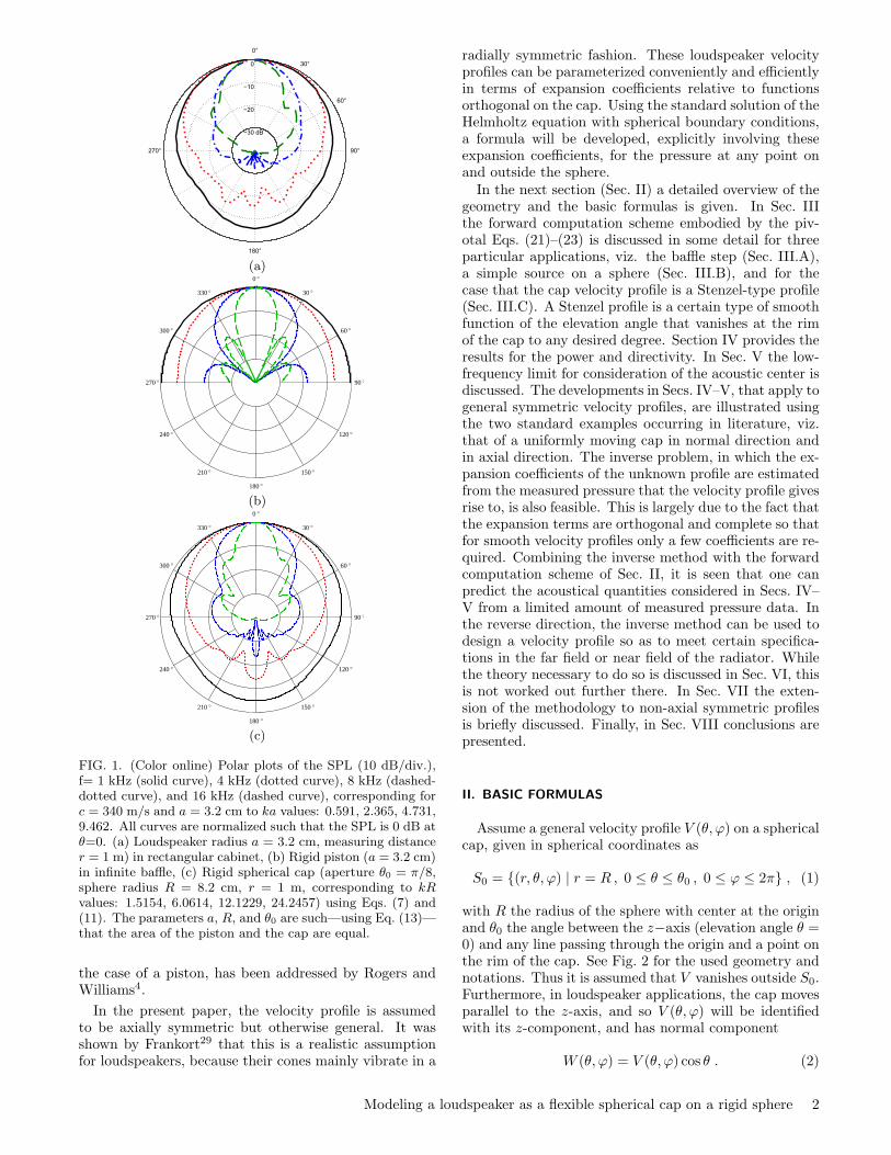
of the sphere is such that the sphere and cabinet havecomparable volumes, respectively 2.3 and 3.1 liters. If Ris such that the sphere volume is the same as that of thecabinet, and θ0 such that the area of the piston and thecap are equal, one gets R = 9.0873 cm and θ0 = 0.35399.The corresponding polar plot—not shown here—is verysimilar to Fig. 1-c, the deviations are about 1 dB or less.Apparently, the actual value of the volume is of modestinfluence. If we keep R fixed and change the cap area bychanging the aperture θ0 however, the influence can besignificant. To illustrate this, polar plots are shown inFig. 3 for constant V , using Eqs. (7) and (11). Figure 3clearly shows that for increasing aperture until, say, θ0 =π/2, the radiation becomes more directive. However, inthe limit case θ0 = π there is only one non-zero Wn

in Eqs. (10) and (11), viz. Wn = δ0n for constant Wand Wn = δ1n for constant V (δ: Kronecker’s delta),respectively. In the case of constant W this is a non-directive pulsating sphere. In the case of constant V weget

p(r, θ) = −iρ0c V cos θh

(2)1 (kr)

h(2)′

1 (kR), (14)

plotted in Fig. 4. This case is discussed in Ref.27 (Sec. 4.-2) as the transversely oscillating rigid sphere. It is readilyseen that p(r, θ)/p(r, 0) = cos θ.

It should be noted that the Wn in Eqs. (10) and (11)have poor decay, roughly like n−1/2, and this shows thatthe representation of W through its Legendre coefficientsis highly inefficient. While poor decay of Wn in Eq. (7)is not necessarily a problem for the forward problem(where the pressure p is computed from W using Eqs. (7)and (9)), it certainly is so for the inverse problem. In theinverse problem, one aims at estimating the velocity pro-file W (or V ) from pressure measurements around thesphere. This can be done, in principle, by adopting amatching approach in Eq. (7) in which the Wn are opti-mized with respect to match of the measured pressure pand the theoretical expression for p in Eq. (7) involvingthe Wn. Even for the simplest case where W is constant,it is seen from the poor decay of the Wn and the poordecay of Pn(cos θ) that a very large number of terms arerequired in the Legendre series in Eq. (8).

In this paper a more efficient representation of W isemployed. This representation uses orthogonal functionson the cap that are derived from Zernike terms

R02`(ρ) = P`(2ρ2 − 1) , 0 ≤ ρ ≤ 1 , ` = 0, 1, · · · , (15)

that were also used in Refs.18–20. See, in particular,Ref.20, Sec. 2 for motivation of this choice. Because ofthe geometry of the spherical cap, a variable transforma-tion is required to pass from orthogonal functions R0

2` onthe disk to orthogonal functions on the cap. In Ref.20,Appendix A, it is shown that the functions

R02`

( sin 12θ

sin 12θ0

), 0 ≤ θ ≤ θ0 , ` = 0, 1, · · · , (16)

are orthogonal on the cap. With

θ = 2 arcsin(s0ρ) ; s0 = sin12θ0 , (17)

0 °

30 °

60 °

90 °

120 °

150 °

180 °

210 °

240 °

270 °

300 °

330 °

(a) θ0 =π/160 °

30 °

60 °

90 °

120 °

150 °

180 °

210 °

240 °

270 °

300 °

330 °

(b) θ0 =2π/160 °

30 °

60 °

90 °

120 °

150 °

180 °

210 °

240 °

270 °

300 °

330 °

(c) θ0 =3π/160 °

30 °

60 °

90 °

120 °

150 °

180 °

210 °

240 °

270 °

300 °

330 °

(d) θ0 =4π/16

FIG. 3. (Color online) Polar plots of the SPL (10 dB/div.),f= 1 kHz (solid curve), 4 kHz (dotted curve), 8 kHz (dashed-dotted curve), and 16 kHz (dashed curve), Rigid spherical capfor various aperture θ0, (sphere radius R = 8.2 cm, r = 1 m)using Eqs. (7) and (11). All curves are normalized such thatthe SPL is 0 dB at θ=0.


0 °

30 °

60 °

90 °

120 °

150 °

180 °

210 °

240 °

270 °

300 °

330 °

FIG. 4. Polar plot for a sphere (θ0 = π) moving with constantvelocity V in the z-direction, using Eqs. (7) and (11). In thiscase W1 = 1, Wn is equal to zero for all values n 6= 1.

the inverse of the variable transformation used inEq. (16), it follows then by orthogonality of the Zerniketerms that

W (2 arcsin(s0ρ)) = w0

∞∑`=0

u`R02`(ρ) , 0 ≤ ρ ≤ 1 , (18)

where the expansion coefficients w0u` are given by

w0u` = 2(2`+ 1)∫ 1

0

W (2 arcsin(s0ρ))R02`(ρ)ρdρ . (19)

It is this parametrization of W in terms of the expansioncoefficients u` that will be preferred in the sequel. Thisparametrization is obtained by ‘warping’ W according toEq. (17) and expanding the warped function as Eqs. (18)–(19) with s0 as in Eq. (17).

The efficiency of the representation in Eq. (18) isapparent from the fact that a smooth profile W re-quires only a limited number of coefficients u` of rel-atively small amplitude yield an accurate approxima-tion of W (2 arcsin(s0ρ)). For instance, the constant pro-file W = w0 on S0 is represented exactly by only oneterm w0R

00(ρ) in the expansion in Eq. (18), and the pro-

file W = v0 cos θ, corresponding to the case that V isconstant v0 on S0, is represented exactly by two termsv0[(1− s20)R0

0(ρ)− s20R02(ρ)]. More complicated examples

arise when V or W is a multiple of the Stenzel profile

(n+ 1)(cos θ − cos θ0

1− cos θ0

)n, (20)

and these require n + 1 terms in the representation inEq. (18). These profiles vanish at the rim of S0 to degreen and are considered in Sec. III.C and VI to illustratethe methods developed in this paper.

It it shown20 that the expansion in Eq. (18) gives riseto a series expression for the pressure p in the whole spaceoutside and on the sphere. The main result is that forr ≥ R, θ ∈ [0, π] and ϕ ∈ [0, 2π]

p(r, θ, ϕ) = −iρ0cw0

∞∑`=0

u`S`(r, θ) , (21)

where

S`(r, θ) =∞∑n=`

(−1)ns0(R2`+12n+1(s0)−R2`+1

2n−1(s0))Pn(cos θ) h(2)n (kr)

h(2)′n (kR)

,

(22)in which

Rmn (ρ) = ρmP(0,m)n−m

2(2ρ2 − 1) , (23)

for integer n,m ≥ 0 with n −m even and ≥ 0 (Rmn ≡ 0otherwise) with P

(α,β)k (x) the general Jacobi polyno-

mial30. These polynomials Rmn (ρ) are called Zernikepolynomials in optics32,33 and they were introduced re-cently in acoustics as well18. This main result providesthe generalization of the forward computation scheme inEqs. (7), (10), (11) to general axially symmetric velocityprofiles W . Furthermore, it provides the basis for theinverse problem, in which the expansion coefficients u`are estimated from measured pressure data around thesphere by adopting a best match approach in Eq. (21).From these estimated coefficients an estimate of W canbe made on basis of Eq. (18). The matter of convergenceof the series in Eq. (22) and some computational issuesare addressed elsewhere20. An alternative way20 to cal-culate the pressure p(r, θ) is by using Eq. (7), where theWn are now given by

Wn = (−1)ns0w0

n∑`=0

(R2`+12n+1(s0)−R2`+1

2n−1(s0))u` , (24)

rather than Eq. (9). This is particularly interesting forthe forward computation scheme with velocity profilesthat vanish smoothly at the rim of the cap as these re-quire only a limited number of terms in Eq. (7).

III. APPLICATIONS OF THE MAIN RESULT

In this section the main result in Eqs. (21)–(23) is illus-trated by considering three applications, viz. the bafflestep, simple source on a sphere, and Stenzel velocity pro-files.

A. Special case baffle step

At low frequencies the baffle of a loudspeaker is smallcompared to its wavelength and radiates due to diffrac-tion effects in the full space (4π-field). At those low fre-quencies the radiator does not benefit from the baffle interms of gain. At high frequencies the loudspeaker ben-efits from the baffle which yields a gain of 6 dB. Thistransition is the well-known baffle step. The center fre-quency of this transition depends on the size of the baffle.Olson31 has documented this for twelve different loud-speaker enclosures, including the sphere, cylinder, andrectangular parallelepiped. All those twelve enclosuresshare the common feature of increasing gain by about6 dB when the frequency is increased from low to high.The exact shape of this step depends on the particular


enclosure. For spheres the transition is smoothest, whilefor other shapes undulations are manifest, in particularfor cabinets with edgy boundaries. In Fig. 5 the bafflestep is shown for a polar cap (θ0 = π/8) on a sphere ofradius R=0.082 m using Eqs. (7) and (11), for differentobservation angles θ = 0 (solid curve), θ = π/9 (dottedcurve), θ = 2π/9 (dashed-dotted curve), and θ = 3π/9(dashed curve). Compare the curves of Fig. 5 with themeasurements using the experimental loudspeaker dis-cussed in Sec. II. It appears that there is a good re-semblance between the measured frequency response ofthe experimental loudspeaker. The undulations, e.g., forθ = 3π/9 (dashed curve) at 7.4, 10, and 13.4 kHz cor-respond well. Although these undulations are often at-tributed to the non-rigid cone movement of the driveritself, our pictures show that it is mainly a diffractioneffect. Furthermore, it can be observed that even on-axis(θ = 0) there is a gradual decrease of SPL at frequenciesabove about 10 kHz. It can be shown from the asymp-totics of the spherical Hankel functions that for θ = 0,k → ∞, and r � R, the sound pressure p(r, θ) given byEq. (21) decays at least as O(k−1/3). This is in contrastwith a flat piston in an infinite baffle. There, the on-axispressure does not decay. This is discussed further at theend of Sec. IV.A.

B. Special case W is a simple source on S0

If the polar cap aperture θ0 decreases towards 0, thecap acts as a simple source. It follows from Eqs. (21)–(23) and by proper normalization by the cap area AS0 ,using Eq. (12), and the definition of w0 in Eq. (3), that

p(r, θ, ϕ) = −iρ0cw0

∞∑n=0

(2n+ 1)Pn(cos θ)h

(2)n (kr)

h(2)′n (kR)

.

(25)In Fig. 6 the corresponding polar plot is illustrated, wherethe same sphere radius and frequencies are used as inFig. 1-c. It appears that the difference between the re-sponse at θ=0 and π is not large, especially for low fre-quencies. This is discussed further in Sec. V with regardto the acoustic center.

C. Stenzel-type profiles and forward computation

Consider the profile

V (K)(θ) = v(K)0 (K + 1)

(cos θ − cos θ01− cos θ0

)K, 0 ≤ θ ≤ θ0 ,

(26)with V (K)(θ) = 0 for θ0 < θ ≤ π (as usual), K = 0, 1, · · · .Then a simple computation shows that

V (K)(2 arcsin(s0ρ)) = v(K)0 (K + 1)(1− ρ2)K , 0 ≤ ρ ≤ 1 .

(27)

100 200 500 1000 2000 5000 1 ´ 104 2 ´ 104freqHHzL

-20

-10

0

10SPLHdBL

(a)

100 1k 10k−30

−25

−20

−15

−10

−5

0

5

10

(b)

FIG. 5. (Color online) (a) Baffle step of a polar cap (θ0 =π/8) on a sphere of radius R =0.082 m, θ = 0 (solid curve),θ = π/9 (dotted curve), θ = 2π/9 (dashed-dotted curve),and θ = 3π/9 (dashed curve), at distance r = 1 m, usingEqs. (21)–(23). All curves are normalized such that the SPLis 0 dB at 100 Hz. (b) Frequency response of a driver (same asFig. 1-a, a = 3.2 cm) mounted in a square side of a rectangularcabinet with dimensions 13x13x18.6 cm, where the parameteris the observation angle θ. The loudspeaker was measuredin an anechoic room at 1 m distance. The on-axis responsewas normalized to 0 dB at 200 Hz, the other curves werenormalized by the same amount.

0 °

30 °

60 °

90 °

120 °

150 °

180 °

210 °

240 °

270 °

300 °

330 °

FIG. 6. (Color online) Polar plots of the SPL (10 dB/div.) ofa simple source on a sphere of radius R =0.082 m. Frequencyf = 1 kHz (solid curve), 4 kHz (dotted curve), 8 kHz (dashed-dotted curve), and 16 kHz (dashed curve), at distance r =1 m, using Eqs. (25). All curves are normalized such that theSPL is 0 dB at θ=0.


The right-hand side of Eq. (27) is the Stenzel profile,considered extensively in Ref.18. Thus

V (K)(2 arcsin(s0ρ)) = v(K)0

K∑`=0

q(K)` R0

2`(ρ) , 0 ≤ ρ ≤ 1 ,

(28)where

q(K)` = (K+1)(−1)`

2`+ 1`+ 1

(K`

)(K + `+ 1

K

) , ` = 0, 1, · · · ,K .

(29)From

W (K)(θ) = V (K)(θ) cos θ =K+1K+2 (1− cos θ0)V (K+1)(θ) + (cos θ0)V (K)(θ) ,

(30)

it follows that

W (K)(2 arcsin(s0ρ)) = w(K)0

K+1∑`=0

u(K)` R0

2`(ρ) , 0 ≤ ρ ≤ 1 ,

(31)where

w(K)0 =

K + 1 + cos θ0K + 2

v(K)0 , (32)

and, for ` = 0, 1, · · · ,K + 1 ,

u(K)` =

v(K)0

w(K)0

[K + 1K + 2

(1− cos θ0)q(K+1)` + (cos θ0)q(K)

`

].

(33)Thus one can compute the pressure using the formulasin Eqs. (21)–(23) with u` = u

(K)` .

0.1 0.2 0.3 0.4Θ

1

2

3

4W HKL

FIG. 7. (Color online) Stenzel profiles for K=0 (solid curve),K=1 (dotted curve), K=2 (dashed-dotted curve), and K=3(dashed curve), using Eqs. (26) and (30) and θ0 = π/8.

In Fig. 7 Stenzel profiles are plotted for K=0 (solidcurve), K=1 (dotted curve), K=2 (dashed-dotted curve),and K=3 (dashed curve). In Fig. 8 polar plots aredisplayed of the SPL (10 dB/div.) of a spherical cap(θ0 = π/8, R = 8.2 cm, r = 1 m) with various Sten-zel velocity profiles, K=0 (solid curve), K=1 (dotted

curve), K=2 (dashed-dotted curve), and K=3 (dashedcurve), (a) f = 4 kHz, (b) f = 8 kHz. It appears thatthe difference between the various velocity profiles aremore pronounced at higher frequencies. Also, the capbecomes less directive for higher K values because in thelimit K → ∞ it would behave like a simple source ona sphere. Furthermore, it appears that the solid curves(K = 0) for (a) f = 4 kHz and (b) f = 8 kHz are the sameas the dotted and dashed-dotted curves, respectively inFig. 1-c. Note that Figs. 1-c and 8 were produced usingtwo different sets of formulas, viz. Eqs. (7) and (11) forFig. 1-c and Eqs. (21) and (33) for Fig. 8, and that theyyield the same plots.

0 °

30 °

60 °

90 °

120 °

150 °

180 °

210 °

240 °

270 °

300 °

330 °

(a)0 °

30 °

60 °

90 °

120 °

150 °

180 °

210 °

240 °

270 °

300 °

330 °

(b)

FIG. 8. (Color online) Polar plots of the SPL (10 dB/div.) ofa spherical cap (θ0 = π/8, R = 8.2 cm, r = 1 m) with vari-ous Stenzel velocity profiles, K=0 (solid curve), K=1 (dottedcurve), K=2 (dashed-dotted curve), andK=3 (dashed curve).(a) f = 4 kHz, (b) f = 8 kHz. All curves are normalized suchthat the SPL is 0 dB at θ=0.

IV. POWER AND DIRECTIVITY

The power is defined as the intensity pv∗ integratedover the sphere Sr of radius r ≥ R,

P =∫Sr

pv∗dSr , (34)


where p and v are the pressure and velocity at an arbi-trary point on the sphere. Using Eq. (7) for the pressureand

v =−1ikρ0c

∂p

∂n(35)

we get

v(r, θ, ϕ) =∞∑n=0

Wn Pn(cos θ)h

(2)′

n (kr)

h(2)′n (kR)

. (36)

By the orthogonality of the Legendre polynomials it fol-lows that

P =∫Srpv∗dSr = 2π

∫ π0p(r, θ)v∗(r, θ)r2 sin θdθ =

−iρ0c∑∞n=0

|Wn|2n+1/2

2πr2h(2)′n (kr)(h(2)′

n (kr))∗

|h(2)′n (kR)|2

.

(37)Using Ref.30, Eq. 10.1.6,

W{jn(z), yn(z)} = jn(z)y′n(z)− j′n(z)yn(z) =1z2, (38)

where W in Eq. (38) denotes the Wronskian, we get

<[P ] =2πρ0c

k2

∞∑n=0

|Wn|2

(n+ 1/2)|h(2)′n (kR)|2

. (39)

Note that Eq. (39) has been derived without using any(near-field or far-field) approximation. The real part ofthe acoustical power is independent of r, which is in ac-cordance with the conservation of power law. For lowfrequencies Eq. (39) is approximated as

<[P ] = 4πρ0cW20 k

2R4 . (40)

To illustrate Eq. (39), the normalized power <[P ]2πρ0cv20R

2

is plotted in Fig. 9, where a cap with various apertures,θ0 = 5π/32 (solid curve), θ0 = π/8 (dotted curve), andθ0 = π/10 (dashed-dotted curve) is moving with a con-stant velocity v0 (using Eq. (10)).

Next, we compare the calculated power with the powermeasured in a reverberation room using the experimen-tal loudspeaker discussed in Sec. II. Here we assumedthe pole cap moving with a constant acceleration (a0 =ikcv0)—corresponding with a frequency independent cur-rent of a constant amplitude through the loudspeaker.Figure 10 shows plots of the calculated power for a rigidspherical cap moving with a constant acceleration andvarious apertures, θ0 = 5π/32 (solid curve), θ0 = π/8(dotted curve), and θ0 = π/10 (dashed-dotted curve), to-gether with the power obtained from the measured loud-speaker (dashed-irregular curve). It appears that the cal-culated power for θ0 = π/8 (dotted curve) and the powerfrom the measured loudspeaker (dashed-irregular curve)are quite similar, while there was no special effort doneto obtain a best fit. A slightly larger aperture than the‘round’ value θ0 = π/8, which we use in many exam-ples in the paper, would have resulted in a better fit.The low-frequency behavior of Fig. 10 follows directly bymultiplying Eq. (40) with 1/(kc)2 because of the constantacceleration of the cap.

5 10 15 20kR

0.001

0.002

0.003

0.004

0.005

0.006

0.007ReHPL

FIG. 9. (Color online) The power <[P ]

2πρ0cv20R

2 of a rigid spheri-

cal cap moving with a constant velocity v0 and various aper-tures, θ0 = 5π/32 (solid curve), θ0 = π/8 (dotted curve), andθ0 = π/10 (dashed-dotted curve), sphere radius R = 8.2 cmusing Eqs. (10) and (39).

0.2 0.5 1. 2. 5. 10. 20.kR

50

55

60

65

ReHPL

FIG. 10. (Color online) The power <[P ]c

2πρ0a20R

4 [dB] vs. kR

(log. axis) of a rigid spherical cap moving with a constant ac-celeration and various apertures, θ0 = 5π/32 (solid curve),θ0 = π/8 (dotted curve), and θ0 = π/10 (dashed-dottedcurve), sphere radius R = 8.2 cm using Eqs. (10) and (39),together with power from the measured loudspeaker (dashed-irregular curve). The logarithmic horizontal axis runs fromkR=0.1–20, corresponding to a frequency range from 66 Hz–13.2 kHz.

A. Directivity

The far-field pressure can be calculated by substitutingthe asymptotic value30 (Ch. 10)

h(2)n (kr) ≈ in+1 e−ikr

kr(41)

in Eq. (7), which leads to

p(r, θ) ≈ ρ0ce−ikr

kr

∞∑n=0

inWn

h(2)′n (kR)

Pn(cos θ) . (42)


In Kinsler et al.26 (Sec. 8.9), the far-field relation is writ-ten as

p(r, θ, ϕ) = pax(r)H(θ, ϕ), (43)

in which pax(r) is the pressure at θ = 0, and H(θ, ϕ) isdimensionless with H(0, 0)=1. Since there is no ϕ depen-dence, we delete it. This leads to

pax(r) = ρ0ce−ikr

kr

∞∑n=0

inWn

h(2)′n (kR)

, (44)

and

H(θ) =p(r, θ)pax(r)

=

∑∞n=0

inWn

h(2)′n (kR)

Pn(cos θ)∑∞n=0

inWn

h(2)′n (kR)

. (45)

The total radiated power Π in the far field follows fromEq. (34) and the far-field relation v = p/(ρ0c) as

Π =∫Sr

1ρ0c|p|2dSr =

1ρ0c|pax(r)|2r2

∫ 2π

0

∫ π0|H(θ, ϕ)|2 sin θ dθ dϕ .

(46)

For a simple (non-directive) source at the origin toyield the same acoustical power on Sr, the pressure psshould satisfy

Π =1ρ0c

4πr2|ps(r)|2 . (47)

Therefore, the directivity defined as

D = |pax(r)|2/|ps(r)|2 , (48)

follows from Eqs. (46) and (47), using the orthogonalityof the Legendre polynomials, as

D =2|∑∞n=0

in+1Wn

h(2)′n (kR)

|2∑∞n=0

|Wn|2

(n+1/2)|h(2)′n (kR)|2

. (49)

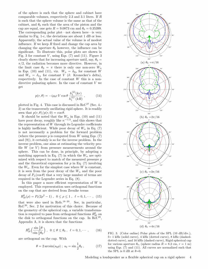
The directivity index DI = 10 log10D [dB] vs. kR isplotted in Fig. 11. For comparison the directivity

Drp =(ka)2

1− J1(2ka)/ka(50)

of a rigid piston in an infinite baffle26 is plotted in Fig. 11(with ka = kR/2.5, so that the π/8-cap and piston havethe same area), as the light-long-dashed curve startingat 3 dB. At low frequencies the directivity Drp is 3 dBbecause the piston is radiating in the 2π-field, while thecaps are radiating in the 4π-field. At higher frequenciesthe curve almost coincides with the dotted curve whichcorresponds to the θ0 = π/8 cap.

Now consider the case that kR → ∞. Then usingh

(2)′

n (kR) ≈ ine−ikR/kR , it follows that D is approxi-mated by

D ≈2|∑∞n=0Wn|2∑∞

n=0|Wn|2

(n+1/2)

=2|W (θ = 0)|2∫ π

0|W (θ)|2 sin θdθ

, (51)

0.2 0.5 1. 2. 5. 10. 20.kR

5

10

15

20DI

FIG. 11. (Color online) The directivity index DI =10 log10D [dB] vs. kR (log. axis) of a rigid spherical capwith various apertures, θ0 = 5π/32 (solid curve), θ0 = π/8(dotted curve), and θ0 = π/10 (dashed-dotted curve), andsphere radius R = 8.2 cm using Eqs. (10) and (49). Thelight-long-dashed curve starting at 3 dB is the directivity fora rigid piston in an infinite baffle, using Eq. (50). The loga-rithmic horizontal axis runs from kR=0.1–25, correspondingto a frequency range from 66 Hz–16.5 kHz.

or, in words, by the ratio of |W (θ = 0)|2 and the aver-age value of |W (θ)|2 over the sphere. Equations (49) and(51) show that the directivity—which is a typical far-field acoustical quantity—is fully determined in a simplemanner by the velocity profile of the pole cap, which canbe easily derived from measurements, e.g., with a laser-Doppler meter. This procedure is not elaborated here. Asimilar result was obtained for a flexible radiator in aninfinite flat baffle19. In the flat baffle case the directivityincreases with (ka)2. For the cap case, there is indeed aninitial increase with (kR)2, but at very high frequencies,there is a decrease of the directivity. These high frequen-cies are in most cases out of the audio range, but maybe of importance for ultrasonics. The deviation of the(kR)2-behavior appears in Fig. 11 for θ0 as low as 5π/32(solid curve). This effect may seem counterintuitive oreven non-physical, however, the on-axis (θ = 0) pressuredecreases for high frequencies as well (see Fig. 5). Thiswill decrease the numerator in Eq. (48) of the directivity.This effect does not occur with a piston in an infinite baf-fle, which has a constant, non-decreasing on-axis soundpressure, but a narrowing beam width.

V. THE ACOUSTIC CENTER

The acoustic center of a reciprocal transducer can bedefined as the point from which spherical waves seem tobe diverging when the transducer is acting as a source.There are more definitions, however, see Ref.34 for anoverview and discussion. This concept is mainly used formicrophones. Recently, the acoustic center was elabo-rated35 for normal sealed-box loudspeakers as a partic-ular point that acts as the origin of the low-frequencyradiation of the loudspeaker. At low frequencies, the ra-diation from such a loudspeaker becomes simpler as the


wavelength of the sound becomes larger relative to theenclosure dimensions, and the system behaves externallyas a simple source (point source). The difference fromthe origin to the true acoustic center is denoted as ∆. Ifp(r, 0) and p(r, π) are the sound pressure in front and atthe back of the source, respectively, then ∆ follows from

|p(r, 0)|r + ∆

=|p(r, π)|r −∆

, (52)

as

∆ = r|q| − 1|q|+ 1

, (53)

where

q = p(r, 0)/p(r, π). (54)

The pole-cap model is used to calculate the function q

æ

æ

æ

æ

æ

æ

æ

æ

æ

0.05 0.1 0.5 1. 5. 10.kR

5

10

15

20

25

30

35

qHdBL

FIG. 12. (Color online) The function 20 log10 |q| [dB] vs.kR (log. axis) given by Eq. (54) of a rigid spherical cap withvarious apertures, θ0 = 5π/32 (solid curve), θ0 = π/8 (dottedcurve), and θ0 = π/10 (dashed-dotted curve), using Eqs. (7)and (11), and a simple source on a sphere using Eq. (25)(dashed curve), all at r = 1 m and sphere radius R = 8.2 cm.The solid circles are from a real driver (same as Fig. 1-a, a =3.2 cm) mounted in a square side of a rectangular cabinet.The logarithmic horizontal axis runs from kR=0.02–30, cor-responding to a frequency range from 13 Hz–19.8 kHz.

via Eq. (7), see Fig. 12. Subsequently, this model is usedto compute the acoustic center with Eq. (53). Assumethat kR� 1 and R/r � 1, and also that Wn is real withWn of at most the same order of magnitude as W0. Thentwo terms of the series in Eq. (7) are sufficient, and usingPn(1) = 1 and Pn(−1) = (−1)n, q can be written as

q ≈(W0

h(2)0 (kr)

h(2)′0 (kR)

+W1h(2)1 (kr)

h(2)′1 (kR)

)/(W0

h(2)0 (kr)

h(2)′0 (kR)

−W1h(2)1 (kr)

h(2)′1 (kR)

).

(55)

Because kR � 1, the small argument approximation ofthe spherical Hankel functions

h(2)′

0 (z) ≈ −iz2, h

(2)′

1 (z) ≈ −2iz3

, (56)

can be used, and together with the identity

h(2)1 (kr)

h(2)0 (kr)

=1kr

(1 + ikr) , (57)

we get

q ≈(

1+W1

2W0(1+ikr)

R

r

)/(1− W1

2W0(1+ikr)

R

r

). (58)

By our assumptions we have | W12W0

(1+ ikr)Rr | � 1 and so

q ≈ 1 +W1

W0

R

r(1 + ikr) . (59)

Finally, assuming that (kr)2 � 2|W0W1| rR , there holds

|q| ≈ 1 +W1

W0

R

r, (60)

and if W1RW0r

� 1 there holds

ϕq = arg q ≈ arctanW1

W0

ωR

c, (61)

where it has been used that W1/W0 is real and k = ω/c.Substitution of Eq. (60) into Eq. (53) results in

∆ ≈ R W1

2 W0. (62)

Note that this result is real, independent of k and r, andonly mild assumptions were used. The delay betweenthe front and at the back of the source is equal to τ =dϕq/dω. Using Eqs. (61) and (62), and assuming kR �W0W1

we get

τ ≈ 2∆c. (63)

For the case W is constant the Wn follow from Eq. (10)resulting in

∆ ≈ 34R(1 + cos θ0) . (64)

If θ0 = π and W is constant, the radiator is a pulsatingsphere, and has according to Eq. (64) its acoustical centerat the origin. For the case V is constant the Wn followfrom Eq. (11) resulting in

∆ ≈ R(

cos θ0 +1

1 + cos θ0

). (65)

If θ0 = π and V is constant, the notion of acoustical cen-ter does not make sense, because of the notches in the po-lar plot at low frequencies, see Fig. 4. The absolute errorin the approximation of ∆/R by Eq. (65) (for f=1 Hz,R=8.2 cm, r=100 m, and 0 ≤ θ0 ≤ π/2) is < 5 10−7.Figure 12 shows that for that case the low-frequencyasymptote is flat to about kR = 0.4 corresponding to264 Hz. Hence the approximation of ∆/R by Eq. (65) israther accurate up to this frequency. The relative acous-tic center difference ∆/R vs. θ0 is plotted in Fig. 13 for


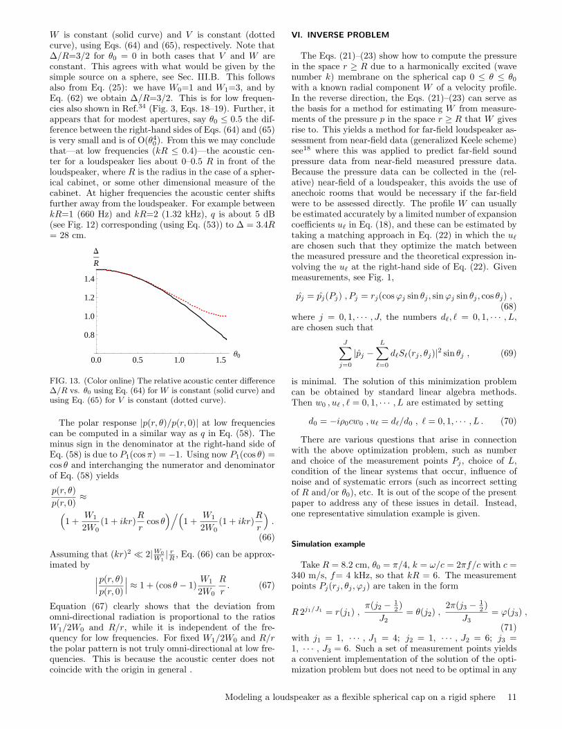
W is constant (solid curve) and V is constant (dottedcurve), using Eqs. (64) and (65), respectively. Note that∆/R=3/2 for θ0 = 0 in both cases that V and W areconstant. This agrees with what would be given by thesimple source on a sphere, see Sec. III.B. This followsalso from Eq. (25): we have W0=1 and W1=3, and byEq. (62) we obtain ∆/R=3/2. This is for low frequen-cies also shown in Ref.34 (Fig. 3, Eqs. 18–19). Further, itappears that for modest apertures, say θ0 ≤ 0.5 the dif-ference between the right-hand sides of Eqs. (64) and (65)is very small and is of O(θ40). From this we may concludethat—at low frequencies (kR ≤ 0.4)—the acoustic cen-ter for a loudspeaker lies about 0–0.5 R in front of theloudspeaker, where R is the radius in the case of a spher-ical cabinet, or some other dimensional measure of thecabinet. At higher frequencies the acoustic center shiftsfurther away from the loudspeaker. For example betweenkR=1 (660 Hz) and kR=2 (1.32 kHz), q is about 5 dB(see Fig. 12) corresponding (using Eq. (53)) to ∆ = 3.4R= 28 cm.

0.0 0.5 1.0 1.5Θ0

0.8

1.0

1.2

1.4

D

R

FIG. 13. (Color online) The relative acoustic center difference∆/R vs. θ0 using Eq. (64) for W is constant (solid curve) andusing Eq. (65) for V is constant (dotted curve).

The polar response |p(r, θ)/p(r, 0)| at low frequenciescan be computed in a similar way as q in Eq. (58). Theminus sign in the denominator at the right-hand side ofEq. (58) is due to P1(cosπ) = −1. Using now P1(cos θ) =cos θ and interchanging the numerator and denominatorof Eq. (58) yields

p(r, θ)p(r, 0)

≈(1 +

W1

2W0(1 + ikr)

R

rcos θ

)/(1 +

W1

2W0(1 + ikr)

R

r

).

(66)

Assuming that (kr)2 � 2|W0W1| rR , Eq. (66) can be approx-

imated by ∣∣∣p(r, θ)p(r, 0)

∣∣∣ ≈ 1 + (cos θ − 1)W1

2W0

R

r. (67)

Equation (67) clearly shows that the deviation fromomni-directional radiation is proportional to the ratiosW1/2W0 and R/r, while it is independent of the fre-quency for low frequencies. For fixed W1/2W0 and R/rthe polar pattern is not truly omni-directional at low fre-quencies. This is because the acoustic center does notcoincide with the origin in general .

VI. INVERSE PROBLEM

The Eqs. (21)–(23) show how to compute the pressurein the space r ≥ R due to a harmonically excited (wavenumber k) membrane on the spherical cap 0 ≤ θ ≤ θ0with a known radial component W of a velocity profile.In the reverse direction, the Eqs. (21)–(23) can serve asthe basis for a method for estimating W from measure-ments of the pressure p in the space r ≥ R that W givesrise to. This yields a method for far-field loudspeaker as-sessment from near-field data (generalized Keele scheme)see18 where this was applied to predict far-field soundpressure data from near-field measured pressure data.Because the pressure data can be collected in the (rel-ative) near-field of a loudspeaker, this avoids the use ofanechoic rooms that would be necessary if the far-fieldwere to be assessed directly. The profile W can usuallybe estimated accurately by a limited number of expansioncoefficients u` in Eq. (18), and these can be estimated bytaking a matching approach in Eq. (22) in which the u`are chosen such that they optimize the match betweenthe measured pressure and the theoretical expression in-volving the u` at the right-hand side of Eq. (22). Givenmeasurements, see Fig. 1,

pj = pj(Pj) , Pj = rj(cosϕj sin θj , sinϕj sin θj , cos θj) ,(68)

where j = 0, 1, · · · , J, the numbers d`, ` = 0, 1, · · · , L,are chosen such that

J∑j=0

|pj −L∑`=0

d`S`(rj , θj)|2 sin θj , (69)

is minimal. The solution of this minimization problemcan be obtained by standard linear algebra methods.Then w0 , u` , ` = 0, 1, · · · , L are estimated by setting

d0 = −iρ0cw0 , u` = d`/d0 , ` = 0, 1, · · · , L . (70)

There are various questions that arise in connectionwith the above optimization problem, such as numberand choice of the measurement points Pj , choice of L,condition of the linear systems that occur, influence ofnoise and of systematic errors (such as incorrect settingof R and/or θ0), etc. It is out of the scope of the presentpaper to address any of these issues in detail. Instead,one representative simulation example is given.

Simulation example

Take R = 8.2 cm, θ0 = π/4, k = ω/c = 2πf/c with c =340 m/s, f= 4 kHz, so that kR = 6. The measurementpoints Pj(rj , θj , ϕj) are taken in the form

R 2j1/J1 = r(j1) ,π(j2 − 1

2 )J2

= θ(j2) ,2π(j3 − 1

2 )J3

= ϕ(j3) ,

(71)with j1 = 1, · · · , J1 = 4; j2 = 1, · · · , J2 = 6; j3 =1, · · · , J3 = 6. Such a set of measurement points yieldsa convenient implementation of the solution of the opti-mization problem but does not need to be optimal in any


other respect (not aimed at here, as said). The profile Wis chosen to be

W (K)(θ) = V (K)(θ) cos θ , 0 ≤ θ ≤ θ0 , (72)

where V (K)(θ) is the Kth Stenzel-type profile as inSec. III.C (see Eqs. (26), (30)), and K = 2. We requirefor this example v0 = v

(K)0 = 1 m/s, and by Eqs. (32)

and (33) we get respectively w0 = w(K)0 and

u(K)` = K+2

K+1+cos θ0

[K+1K+2 (1− cos θ0)q(K+1)

` + (cos θ0)q(K)`

].

(73)Using q

(K+1)` , q(K)

` given by Eq. (29), the pressure p iscomputed in accordance with Eq. (21) with u` = u

(K)` .

Measurements pj are obtained in simulation by addingcomplex white noise (SNR= 40 dB) to the computedp(Pj). The non-zero coefficients of W (K) are estimatedby taking L = K + 1 in the optimization problem,and this yields estimates w0, u0, · · · , uK+1 of w0,u0, · · · , uK+1. Figure 14 for the case K=2 shows theStenzel profile W (K) of Eq. (72) using Eq. (20) directly(solid curve) together with the reconstructed profiles

W (K)(θ) = w(K)0

K+1∑`=0

u`R02`

( sin 12θ

sin 12θ0

), 0 ≤ θ ≤ θ0 ,

(74)without noise (dotted curve) and with noise (dashed-dotted curve) added to the pressure points pj . The re-covered u` are computed by solving Eq. (69) and usingEqs. (70), (31), and Eqs.(16)–(18). Figure 14 shows thatthe (noiseless) reconstructed profile (dotted curve) coin-cides with the Stenzel profile (solid curve), and that therecovered profile using the noisy pressure points (dashed-dotted curve) is very similar to the other two curves. Themethod appears to be robust for noise contamination.Figure 15 shows the corresponding polar plot of the ve-locity profile of Fig. 14. The solid curve in Fig. 15 is forthe near field (r = 0.0975 m) and the dotted curve forthe far- field (r = 1 m). It appears that the near field ismore directive than the far field.

VII. EXTENSION TO NON-AXIALLY SYMMETRICPROFILES

Loudspeaker membranes vibrate mainly in a radiallysymmetric fashion, in particular at low frequencies. Athigher frequencies, break-up behavior can become man-ifest, and then it may be necessary to consider non-radially symmetric profiles. In the present context, wherea loudspeaker is modeled as consisting of a rigid spher-ical cabinet with a flexible spherical cap, this requiresconsideration of non-axially symmetric velocity profilesV (θ, ϕ) and W (θ, ϕ) on S0. This is beyond the scope ofthe present paper and is discussed elsewhere20.

VIII. CONCLUSIONS

Appropriately warped Legendre polynomials providean efficient and robust method to describe velocity pro-

0.2 0.4 0.6 0.8Θ

0.2

0.4

0.6

0.8

1.0W HKL

FIG. 14. (Color online) Stenzel profile W (K)/(K+ 1) (K = 2and θ0 = π/4) of Eq. (72) using Eq. (20) directly (solid curve)

together with the reconstructed profiles W (K) without noise(dotted curve) and with noise added to the pressure points pj(dashed-dotted curve). The (noiseless) reconstructed profile(dotted curve) coincides with the input profile (solid curve).

0 °

30 °

60 °

90 °

120 °

150 °

180 °

210 °

240 °

270 °

300 °

330 °

FIG. 15. (Color online) Polar plots (10 dB/div.) in the nearfield (solid curve, r = 0.0975 m) and in the far field (dottedcurve, r = 1 m), corresponding to the parameters of the sim-ulation example and the velocity profile of Fig. 14. All curvesare normalized such that the SPL is 0 dB at θ=0.

files of a flexible spherical cap on a rigid sphere. Only afew coefficients are necessary to approximate various ve-locity profiles. The polar plot of a rigid spherical cap ona rigid sphere has been shown to be quite similar to thatof a real loudspeaker, and is useful in the full 4π-field.The spherical-cap model yields polar plots that exhibitgood full range similarity with the polar plots from realloudspeakers. It thus outperforms the more conventionalmodel in which the loudspeaker is modeled as a rigidpiston in an infinite baffle. The cap model can be usedto predict, besides polar plots, various other acousticalquantities of a loudspeaker. These quantities include thesound pressure, baffle-step response, sound power, direc-tivity, and the acoustic center. At low frequencies (kR ≤0.4) the acoustic center for a loudspeaker lies about 0–0.5 R in front of the loudspeaker, where R is the radius


in the case of a spherical cabinet, or some other dimen-sional measure of the cabinet. At higher frequencies theacoustic center shifts further away from the loudspeaker.The method presented herein enables one to solve the in-verse problem of calculating the actual velocity profile ofthe cap radiator using (measured) on- and off-axis soundpressure data. This computed velocity profile allows theextrapolation to far-field loudspeaker pressure data, in-cluding off-axis behavior. Because the pressure data canbe collected in the (relative) near-field of a loudspeaker,this avoids the use of anechoic rooms that would be nec-essary if the far-field were to be assessed directly.

Acknowledgments

The authors wish to thank Okke Ouweltjes for assistingin the loudspeaker measurements and making the plot forFig. 1a, and Prof. Fred Simons for providing pertinentassistance in programming Mathematica, in particular tomake Fig. 14.

1 J.W.S. Rayleigh. The Theory of Sound, Vol. 2, 1896.(reprinted by Dover, New York), 1945.

2 L.V. King. On the acoustic radiation field of the piezo-electric oscillator and the effect of viscosity on transmis-sion. Can. J. Res., 11:135–155, 1934.

3 A. Schoch. Contemplations on the sound field of pistonmembranes (published in German as Betrachtungen uberdas Schallfeld einer Kolbenmembran). Akust. Z. 6, 318-326(1941).

4 Peter H. Rogers, and A.O. Williams, Jr. Acoustic field ofcircular plane piston in limits of short wavelength or largeradius. J. Acoust. Soc. Am., 52(3B):865–870, 1972.

5 M. Greenspan. Piston radiator: Some extensions of thetheory. J. Acoust. Soc. Am., 65(3):608–621, 1979.

6 G.R. Harris. Review of transient field theory for a baffledplanar piston. J. Acoust. Soc. Am., 70(1):10–20, 1981.

7 R. New, R.I. Becker, and P. Wilhelmij. A limiting formfor the nearfield of the baffled piston. J. Acoust. Soc. Am.,70(5):1518-1526, Nov. 1981.

8 T. Hasegawa, N. Inoue, and K. Matsuzawa. A new rigorousexpansion for the velocity potential of a circular pistonsource. J. Acoust. Soc. Am., 74(3):1044–1047, September1983.

9 D.A. Hutchins, H.D. Mair, P.A. Puhach, and A.J. Osei.Continuous-wave pressure fields of ultrasonic transducers.J. Acoust. Soc. Am., 80(1):1–12, July 1986.

10 R. C. Wittmann, and A. D. Yaghjian. Spherical-wave ex-pansions of piston-radiator fields. J. Acoust. Soc. Am.,90(3):1647–1655, September 1991.

11 R.M. Aarts, and A.J.E.M. Janssen. Approximation of theStruve function H1 occurring in impedance calculations.J. Acoust. Soc. Am., 113(5):2635-2637, May 2003.

12 T. Helie, and X. Rodet. Radiation of a pulsating portionof a sphere: Application to horn radiation. Acta Acusticaunited with Acustica, 89(4), 565–577, July/August 2003

13 R.J. McGough, T.V. Samulski, and J.F. Kelly. An effi-cient grid sectoring method for calculations of the near-field pressure generated by a circular piston. J. Acoust.Soc. Am., 115(5):1942–1954, May 2004.

14 T.D. Mast, and F. Yu. Simplified expansions for radia-tion from a baffled circular piston. J. Acoust. Soc. Am.,118:3457–3464, 2005.

15 T.J. Mellow. On the sound field of a resilient disk in aninfinite baffle. J. Acoust. Soc. Am., 120:90–101, 2006.

16 J.F. Kelly, and R.J. McGough. An annular superpositionintegral for axisymmetric radiators. J. Acoust. Soc. Am.,121:759–765, 2007.

17 Xiaozheng Zeng, and R.J. McGough. Evaluation of the an-gular spectrum approach for simulations of near-field pres-sures. J. Acoust. Soc. Am., 123(1):68–76, January 2008.

18 R.M. Aarts, and A.J.E.M. Janssen. On-axis and far-fieldsound radiation from resilient flat and dome-shaped radia-tors. J. Acoust. Soc. Am., 125(3):1444-1455, March 2009.

19 R.M. Aarts, and A.J.E.M. Janssen. Sound radiation quan-tities arising from a resilient circular radiator. J. Acoust.Soc. Am., 126(4):17761787, Oct. 2009.

20 R.M. Aarts, and A.J.E.M. Janssen. Sound radiation froma resilient spherical cap on a rigid sphere. J. Acoust. Soc.Am., 127(4), April 2010.

21 R.M. Aarts, and A.J.E.M. Janssen. Estimating the ve-locity profile and acoustical quantities of a harmonicallyvibrating loudspeaker membrane from on-axis

22 P.M. Morse, and H. Feshbach. Methods of theoreticalphysics. McGraw-Hill, 1953.

23 H. Stenzel, and O. Brosze. Guide to computation of soundphenomena (published in German as Leitfaden zur Berech-nung von Schallvorgangen), 2nd ed. Springer-Verlag,Berlin, 1958.

24 P.M. Morse, and K.U. Ingard. Theoretical acoustics.McGraw-Hill Book Company, New York, 1968.

25 E. Skudrzyk. The Foundations of Acoustics. Springer-Verlag, New York, 1971, ASA-reprint 2008.

26 L.E. Kinsler, A.R. Frey, A.B. Coppens, and J.V. Sanders.Fundamentals of Acoustics. Wiley, New York, 1982.

27 A.D. Pierce. Acoustics, An Introduction to Its PhysicalPrinciples and Applications. Acoustical Society of Americathrough the American Institue of Physics, 1989.

28 D.T. Blackstock. Fundamentals of physical Acoustics. JohnWiley & Sons, New York, 2000.

29 F.J.M. Frankort. Vibration and Sound Radiation of Loud-speaker Cones. Ph.D. dissertation, Delft University ofTechnology, 1975.

30 M. Abramowitz, and I.A. Stegun. Handbook of Mathemat-ical Functions. Dover, New York, 1972.

31 Harry F. Olson. Direct radiator loudspeaker enclosures. J.Audio Eng. Soc. 17(1), 22–29, Jan. 1969.

32 A.J.E.M. Janssen, and P. Dirksen. Concise formula for theZernike coefficients of scaled pupils. J. Microlith., Micro-fab., Microsyst., 5(3), 030501, July-Sept. 2006.

33 A.J.E.M. Janssen, S. van Haver, P. Dirksen, and J.J.M.Braat. Zernike representation and Strehl ratio of opticalsystems with variable numerical aperture. J. of ModernOptics, 55(7), 1127–1157, April 2008.

34 Finn Jacobsen, Salvador Barrera Figueroa, and Knud Ras-mussen. A note on the concept of acoustic center. J.Acoust. Soc. Am., 115(4):1468–1473, April 2004.

35 John Vanderkooy. The acoustic center: A new concept forloudspeakers at low frequencies. AES Convention paper

6912 presented at the 121th Convention, San Francisco,Oct. 5–8, 2006.


modeling a loudspeaker as a exible spherical cap on a ... · modeling a loudspeaker as a exible...

Documents