modeling and computation of magnetic leakage field in ... · modeling and computation of magnetic...

Modeling and Computation of Magnetic Leakage

Field in Transformer Using Special Finite

Elements

Tarlochan Kaur and Raminder Kaur Electrical Engineering Department of PEC University of Technology, Chandigarh, India

Email: {tarlochankaur, raminderkaur}@pec.ac.in

Abstract—Accuracy in theoretical prediction of performance

of transformers has become increasingly important to effect

economy in design and to ensure reliability of operation.

Some of the performance indicators that the power system

engineers are concerned with are reactance, electromagnetic

forces, short circuit impedance etc. In recent years, finite

element methods have been increasingly used. One of the

drawbacks in the flux plots so obtained is that at all infinitely

permeable iron surface the flux lines are not normal to the

iron surface. To eliminate these errors on the boundaries

special finite elements i.e. incremental curved elements with

linear and cubic variations have been developed. Their

incorporation would modify the usual shape functions. With

the help of modified shape functions the magnetic vector

potentials are solved. Leakage reactance, the magnetic force,

energy is calculated and flux plots obtained.

Index Terms—transformer, power system computing finite

element method flux plots

I. INTRODUCTION

Since one of the important features of a transformer is its

leakage impedance, improvements in the calculations of

this quantity are always searched for. [1]-[3] Analytical

methods have been employed in the past for determining

the actual flux distribution but most of the analytical

methods are not accurate [4], [5]. The drawback of these

representations is either the simplified assumptions or the

complex nature, which makes the use of it impracticable.

Rabin [6] has also presented a solution using Fourier series

representations of the ampere-turns distribution, in axial

directions only. In the transition region between the two

windings, there is an abrupt change in the ampere-turns

distribution, and it is difficult to represent this by Fourier

series accurately. Numerical modeling techniques are

now-a-days well established for transformer analysis and

enable representation of all important features of these

devices [7]-[9]. In the application of finite element

methods for axi- symmetric problems, only the first order

and high order triangular elements have been used [10],

[11] and flux plots obtained. One of the drawbacks in the

flux plots so obtained is that at all infinitely permeable iron

Manuscript received October 16, 2014; revised August 15, 2015.

surface the flux lines are not normal to the iron surface, i.e.

Neumann’s boundary condition is not satisfied as it

constitutes the natural functional. To eliminate these errors

on the boundaries special finite elements i.e. incremental

curved elements with linear and cubic variations have been

developed.

II. TRANSFORMER MODELING WITH FINITE ELEMENT

METHOD

Mathematical formulation: For the purpose of

analysis, the transformer will be assumed rotationally

symmetric about a core leg. It will be assumed that all iron

is infinitely permeable. In the insulation and winding space

the magnetic vector potential must satisfy the vector

Poisson’s equation. The Poisson’s equation in cylindrical

coordinates for axi-symmetric problems can be written as:

rvv J

r r r z z

(1)

Subject to the boundary conditions: is specified on

the part of the boundary S1 and ∂ /∂n on the part of the

boundary S2

In the present formulation the given region is divided

into a mesh of finite elements, and the vector potential

is approximated in each element. The mesh is a set of rings,

each ring having a general curvilinear quadrilateral

cross-section that has been revolved around the z-axis. The

current density, J is assumed to be directed in the

peripheral direction, and thus the vector potential, is

also peripherally directed. Within each element the vector

potential is assumed to vary according to the equation:

i iN (2)

where Ni is the usual shape functions [10] and i is the

nodal values of vector potentials.

III. FORMULATION OF INCREMENTAL ELEMENTS

Fig. 1 (a) and Fig. 1(b) shows para- linear and parabolic

incremental elements respectively where EF is the

boundary on which the condition / ( , )n x y holds.

International Journal of Electronics and Electrical Engineering Vol. 4, No. 3, June 2016

©2016 Int. J. Electron. Electr. Eng. 231doi: 10.18178/ijeee.4.3.231-234

One side of the element, represented by the nodes 4, 5 and

6 is lying on the boundary EF. The opposite side, having

nodes 1, 2 and 3 on it, is lying on the boundary line GH,

which is very close to the boundary line EF. The variations

in the η and ξ directions are linear and parabolic

respectively.

Figure 1. (a) Para-Linear incremental element (b) parabolic incremental

element

Higher or lower variation in ξ direction is possible. Thus

basically an incremental element is either a linear-linear,

para-linear or a cubi- linear element. The shape functions

for the curved para-linear element can be written as:

1 1 1N n ,

2 2 1N n ,

3 3 1N n ,

4 3 2N n ,

5 2 2N n ,

6 1 2N n (3)

where 10.5 1n , 2

21n , 3

0.5 1n ,

1 0.5 1 , and 2

0.5 1

Assuming,

341 , 252 and 163

The usual nodal potential values, e and the

incremental nodal potentials, e

are related by:

eeC (4)

where

100001

010010

001100

000100

000010

000001

C and

Te

321321 ,,,,,,

Matrix [C] is the required connection matrix. The

element in terms of the incremental nodal potentials is

represented in Fig. 1(b). The potential at any point in

para-linear element is given by:

eN

This expression can be modified, with the help of Eq.(4)

to connect the potential, , with the incremental

parameters. Thus:

e

N C

e

N (5)

where N N C = 1 6 2 5 3 4 4 5 6, , , , ,N N N N N N N N N

Let: ' ' '

1 2 3 4 5 6, , , , , ,N N N N N N N (6)

where '

1N ,

'

2N , and

'

3N are the new shape functions at

nodes 1, 2 and 3 respectively, and can be shown to be equal

to:

1

'

1 nN , 2

'

2 nN , 3

'

3 nN (7)

For the calculation of gradient matrix the Jacobin matrix

and its determinant and the original shape functions of the

para- linear element as given by (3) are required. Thus the

modified shape functions, (6) and the original shape

functions, (3) will have to be stored. An alternative

approach is to calculate the Jacobian matrix and its

determinant by using the modified shape functions. For this

the coordinates of the nodes will have to be modified, since

it is convenient to modify the coordinates of the nodes

instead of retaining the original shape functions. This latter

approach is used here. Using the modified shape functions

the x and y coordinates can be written as:

ee

x N x N x

ee

y N y N y (8)

where:

1e e

x C x

1 2 3 1 2 3

, , , , , ,x x x x x x

1e e

y C y

1 2 3 1 2 3

, , , , , ,y y y y y y

and 1 4 3

,x x x 2 5 2

,x x x 3 6 1

,x x x and

so on. x and y

are the modified coordinates of the

element. Only the coordinates of the nodes lying on the

boundary EF needs modifications. With the modified

shape functions and coordinates the procedure of

calculating the element properties by numerical integration

will remain unaltered. The elements fulfill the necessary

conditions of convergence. The compatibility conditions

are also satisfied. The incremental elements must satisfy

the Neumann type of boundary condition ∂ /∂n = α (x, y).

For this purpose α will appear in the final potential vector

of the global equations as the known values of the nodal

potentials for the nodes on the boundary EF. Using

modified shape functions reluctance matrix, [R] and

current load vector {I} is carried out numerically.


©2016 Int. J. Electron. Electr. Eng. 232

IV. REACTANCE CALCULATION

The leakage reactance can be calculated as pointed out

by Anderson [11] and Silvester [12], by calculating the

stored energy in the leakage field. The leakage reactance X,

using the stored energy W, is given by: 2

2 /X W I

where:

0.5 .v

W J dv (9)

ω is supply frequency, and I is the current peak or effective,

for which the energy W was evaluated. For the

axi-symmetric problems, the radial and axial components

of the short circuit electromagnetic force can be written as:

r z

vz r

F BJ dv

F B

(10)

where Bz and Br are the flux densities in axial and radial

directions respectively.

TABLE I. COMPUTED VALUE OF LEAKAGE REACTANCE

V. SAMPLE PROBLEM

Andersen [10] and Silvester [11] have used the Rabins

case 2 to illustrate their finite element analysis. This case is

taken to illustrate the various aspects of the present finite

element analysis. In the analysis numerically integrated

general quadrilateral iso-parametric elements with or

without curved sides have been used. Transformer leakage

field analysis is dealt in the present discussion.

The element having linear, parabolic and cubic

interpolation functions and belonging to serendipity family

have been used. These elements are shown in Fig. 1(a) and

(b). For comparison, the solution domain was divided into

elements so that the total number of nodes are

approximately same for various type of elements. The

results obtained for approximately 100 nodes and 180

nodes are tabulated in Table I.

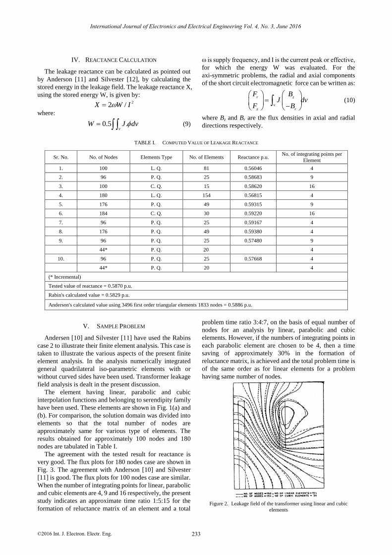
The agreement with the tested result for reactance is

very good. The flux plots for 180 nodes case are shown in

Fig. 3. The agreement with Anderson [10] and Silvester

[11] is good. The flux plots for 100 nodes case are similar.

When the number of integrating points for linear, parabolic

and cubic elements are 4, 9 and 16 respectively, the present

study indicates an approximate time ratio 1:5:15 for the

formation of reluctance matrix of an element and a total

problem time ratio 3:4:7, on the basis of equal number of

nodes for an analysis by linear, parabolic and cubic

elements. However, if the numbers of integrating points in

each parabolic element are chosen to be 4, then a time

saving of approximately 30% in the formation of

reluctance matrix, is achieved and the total problem time is

of the same order as for linear elements for a problem

having same number of nodes.

Figure 2. Leakage field of the transformer using linear and cubic

elements

Sr. No. No. of Nodes Elements Type No. of Elements Reactance p.u. No. of integrating points per

Element

1. 100 L. Q. 81 0.56046 4

2. 96 P. Q. 25 0.58683 9

3. 100 C. Q. 15 0.58620 16

4. 180 L. Q. 154 0.56815 4

5. 176 P. Q. 49 0.59315 9

6. 184 C. Q. 30 0.59220 16

7. 96 P. Q. 25 0.59167 4

8. 176 P. Q. 49 0.59380 4

9. 96 P. Q. 25 0.57480 9

44* P. Q. 20 4

10. 96 P. Q. 25 0.57668 4

44* P. Q. 20 4

(* Incremental)

Tested value of reactance = 0.5870 p.u.

Rabin's calculated value = 0.5829 p.u.

Anderson's calculated value using 3496 first order triangular elements 1833 nodes = 0.5886 p.u.



Figure. 3. Leakage field of the transformer using parabolic elements

The problem was also analyzed by the use of

incremental elements. The 96 Node, 25 parabolic elements

Fig. 2 and Fig. 3, mesh was used by applying the

incremental elements around it. The efficiency and

computational effort are of the same order as that when no

incremental elements are used. The use of incremental

elements has given a reactance value, hence the stored

energy is also slightly less than the tested value. This is due

to the fact that the incremental elements allow the flux

density variation in only one direction and this effect is also

carried to some extent to the normal element on the side of

which the incremental element is attached.

In case of normal elements the solution has been

possible by assuming a known potential at one point in the

domain. In present work zero potential is assumed at lower

left corner. No such assumption is necessary, when field is

analyzed with the help of incremental elements

VI. CONCLUSION

The use of incremental numerically integrated higher

order isoparametric elements offers many significant

advantages. These are easy to use, boundary conditions

and curvatures are properly accounted for; they yield fast

and reliable solutions. On the basis of improved accuracy,

and computational efforts required to solve a given

problem and ease in input data preparation, the parabolic

elements are preferred for routine work. In addition, total

computation time of the order of linear elements is

obtained if parabolic elements with four integrating points

are used. The use of cubic elements is recommended only

in cases where flux concentration is high and the geometry

permits the use of only few elements.

REFERENCES

[1] A. M. Kashtiban, “Finite element calculation of winding type effect

on leakage flux in single phase shell type transformers,” in Proc.

5th WSEAS International Conference on Applications of Electrical

Engineering, Prague, Czech Republic, 2006, pp. 39-43.

[2] M. A. Tsili, “Advanced design methodology for single and dual

voltage wound core power transformers based on a particular finite

element model,” Electric Power Systems Research, vol. 76, pp.

729-741, 2006

[3] A. N. Jahromi, “A fast method for calculation of transformers

leakage reactance using energy technique,” IJE Transactions B:

Applications, vol. 16, no. 1, 2003.

[4]

[5] V. N. Mittit, Design of Electrical Machines, 4th ed., New Delhi: N.

C. Jain for Standard Publishers Distributors, 1996.

[6] L. Rabins, “Transformer reactance calculations with digital

computers,” IEEE Trans., vol. 75, pp. 262-267, 1956.

[7] C. B. Simon and S. B. Pat, “Power transformer design using

magnetic circuit theory and finite element analysis-a comparison of

techniques,” presented at the AUPEC, Perth, Western Australia,

2007.

[8] S. A. Jamali and K. Abbaszadeh, “The study of magnetic flux

shunts effects on the leakage reactance of transformers via FEM,”

Majlesi Journal of Electrical Engineering, vol. 4, no. 3, 2010.

[9] J. D. Layers, “Electromagnetic field computation in power

engineering,” IEEE Trans. on Magnetics, vol. 29, no. 6, 1993.

[10] O. W. Andersen, “Transformer leakage flux program based on the

finite element method,” IEEE Trans., vol. 92, pp. 682-689, 1973.

[11] P. Silvester and A. Konar, “Analysis of transformer leakage

phenomena by high-order finite elements,” IEEE Trans., vol. 92,

pp. 1843-1855, 1973.

Dr. (Mrs.) Tarlochan Kaur was born in India on August 11, 1962. She

received B.E, M.E (Electrical) and Ph.D. (Engg. and Tech.) Engineering

from Panjab University, Chandigarh, India in 1984, 1985 and 1998

respectively. Her area of research interest includes Electromagnetic

Fields, Electric Machines, Power Systems, Renewable Energies and

FACTS. She has to her credit over 50 published research papers in

various International Journals and Conferences. She has contributed

many articles in the newspapers. She is currently working as Head &

Associate Professor in Electrical Engineering Department in PEC

University of Technology, Chandigarh, India.

Mrs. Raminder Kaur was born in India on August 23, 1963. She

received both B.E and M.E in Electrical Engineering from PEC

University of Technology (formerly called Punjab Engineering College),

Chandigarh, India in 1984 and 1990 respectively. Currently she is

pursuing PhD degree in the area of transmission planning in deregulated

environment with distributed generation at the Department of Electrical

Engineering, PEC University of Technology, Chandigarh. She joined

PEC, Chandigarh in April 1992. Since then she has been working as an

Assistant Professor in Department of Electrical Engineering, PEC

University of Technology, Chandigarh.



M. F. William, Handbook of Transformer Design and Application,

2nd ed., McGraw-Hill, 1992.

modeling and computation of magnetic leakage field in ... · modeling and computation of magnetic...

Documents