modeling and control of a magnetic fluid deformable …€¦ · fluid deformable mirror for...
TRANSCRIPT

MODELING AND CONTROL OF A MAGNETIC
FLUID DEFORMABLE MIRROR FOR
OPHTHALMIC ADAPTIVE OPTICS SYSTEMS
by
Azhar Iqbal
A thesis submitted in conformity with the requirementsfor the degree of Doctor of Philosophy
Department of Mechanical and Industrial EngineeringUniversity of Toronto
Copyright c© 2009 by Azhar Iqbal
ABSTRACT
MODELING AND CONTROL OF A MAGNETIC FLUID DEFORMABLE MIRROR
FOR OPHTHALMIC ADAPTIVE OPTICS SYSTEMS
Azhar Iqbal
Doctor of Philosophy
Department of Mechanical and Industrial Engineering
University of Toronto
2009
Adaptive optics (AO) systems make use of active optical elements, namely wavefront
correctors, to improve the resolution of imaging systems by compensating for complex
optical aberrations. Recently, magnetic fluid deformable mirrors (MFDM) were proposed
as a novel type of wavefront correctors that offer cost and performance advantages over
existing wavefront correctors. These mirrors are developed by coating the free surface
of a magnetic fluid with a thin reflective film of nano-particles. The reflective surface
of the mirrors can be deformed using a locally applied magnetic field and thus serves
as a wavefront corrector. MFDMs have been found particularly suitable for ophthalmic
imaging systems where they can be used to compensate for the complex aberrations in
the eye that blur the images of the internal parts of the eye. However, their practical
implementation in clinical devices is hampered by the lack of effective methods to control
the shape of their deformable surface.
The research work reported in this thesis presents solutions to the surface shape
control problem in a MFDM that will make it possible for such devices to become in-
tegral components of retinal imaging AO systems. The first major contribution of this
research is the development of an accurate analytical model of the dynamics of the mir-
ror surface shape. The model is developed by analytically solving the coupled system
of fluid-magnetic equations that govern the dynamics of the surface shape. The model
is presented in state-space form and can be readily used in the development of surface
shape control algorithms. The second major contribution of the research work is a novel,
ii

innovative design of the MFDM. The design change was prompted by the findings of
the analytical work undertaken to develop the model mentioned above and is aimed at
linearizing the response of the mirror surface. The proposed design also allows for mirror
surface deflections that are many times higher than those provided by the conventional
MFDM designs. A third contribution of this thesis involves the development of control
algorithms that allowed the first ever use of a MFDM in a closed-loop adaptive optics
system. A decentralized proportional-integral (PI) control algorithm developed based on
the DC model of the wavefront corrector is presented to deal mostly with static or slowly
time-varying aberrations. To improve the stability robustness of the closed-loop AO sys-
tem, a decentralized robust proportional-integral-derivative (PID) controller is developed
using the linear-matrix-inequalities (LMI) approach. To compensate for more complex
dynamic aberrations, an H∞ controller is designed using the mixed-sensitivity H∞ design
method. The proposed model, design and control algorithms are experimentally tested
and validated.
iii

Acknowledgements
I wish to thank my academic supervisor Professor Foued Ben Amara for his guidance,
support and patience during the course of the research work reported in this thesis.
I would also like to acknowledge the assistance and cooperation of my colleagues and
friends Maurizio Ficocelli, Zhizheng (Daniel) Wu, Zhichong (Jason) Li, Qingkun (Tony)
Zhou, Devina Dukhu, Xiaolu Sun, Geoff Fung, Steve Bristo and Ryan Li. Special thanks
to Maurizio for his help in building the experimental setup. I am grateful to Daniel
for providing critical help and advice in the design of controllers. Jason, Devina and
Xiaolu contributed in performing simulations. Tony, thank you for your contribution to
the design of electromagnetic actuator coils. Geoff helped me build the control circuitry.
Steve assisted in the assembly of the optical system. Ryan facilitated the use of magnetic
fluids. Thank you all.
My studies and the research work was partly supported by the Ministry of Science
and Technology, Government of Pakistan and, for that, I remain indebted to the people
of that country.
Last, but not least, I would like to thank my family for all their encouragement and
support throughout my studies.
iv
Contents
1 Introduction 1
1.1 Motivation . . . . . . . . . . . . . . . . . . . . . . . . . . . . . . . . . . . 1
1.2 Objectives . . . . . . . . . . . . . . . . . . . . . . . . . . . . . . . . . . . 4
1.3 Major Contributions . . . . . . . . . . . . . . . . . . . . . . . . . . . . . 5
1.4 Organization of the Thesis . . . . . . . . . . . . . . . . . . . . . . . . . . 6
2 AO Systems and Magnetic Fluid Deformable Mirrors 7
2.1 Introduction to Adaptive Optics Systems . . . . . . . . . . . . . . . . . . 7
2.1.1 The Basic Concept of a Wavefront . . . . . . . . . . . . . . . . . 8
2.1.2 Description of Optical Aberrations . . . . . . . . . . . . . . . . . 8
2.1.3 Representation of Aberrations . . . . . . . . . . . . . . . . . . . . 10
2.1.4 Optical Metrics of Aberrations . . . . . . . . . . . . . . . . . . . . 14
2.1.5 Wavefront Correction . . . . . . . . . . . . . . . . . . . . . . . . . 19
2.1.6 Brief History of Adaptive Optics Systems . . . . . . . . . . . . . . 21
2.1.7 Operating Principle of an Adaptive Optics System . . . . . . . . . 22
2.2 Retinal Imaging Adaptive Optics Systems . . . . . . . . . . . . . . . . . 29
2.2.1 The Structure of the Eye . . . . . . . . . . . . . . . . . . . . . . . 30
2.2.2 Sources of Aberrations in the Eye . . . . . . . . . . . . . . . . . . 32
2.2.3 Dynamics of the Aberrations in the Eye . . . . . . . . . . . . . . 33
2.2.4 Correction of the Aberration in Eye using AO System . . . . . . . 35
v

2.2.5 History of Ophthalmic Adaptive Optics Systems . . . . . . . . . . 38
2.2.6 Challenges to Ophthalmic Adaptive Optics Systems . . . . . . . . 39
2.3 Magnetic Fluid Deformable Mirrors . . . . . . . . . . . . . . . . . . . . . 40
2.3.1 Principle of Operation . . . . . . . . . . . . . . . . . . . . . . . . 40
2.3.2 Brief History of Development of MFDMs . . . . . . . . . . . . . . 42
2.3.3 Magnetic Fluids . . . . . . . . . . . . . . . . . . . . . . . . . . . . 43
2.3.4 MELLFs . . . . . . . . . . . . . . . . . . . . . . . . . . . . . . . . 45
2.3.5 Current State of Research and Challenges . . . . . . . . . . . . . 46
2.3.6 Performance Requirements . . . . . . . . . . . . . . . . . . . . . . 48
2.3.7 Research Goals . . . . . . . . . . . . . . . . . . . . . . . . . . . . 49
2.4 Summary . . . . . . . . . . . . . . . . . . . . . . . . . . . . . . . . . . . 50
3 Analytical Model of a MFDM 51
3.1 Analytical Model in Cartesian Geometry . . . . . . . . . . . . . . . . . . 51
3.1.1 Governing Equations . . . . . . . . . . . . . . . . . . . . . . . . . 52
3.1.2 Simplification of the Governing Equations . . . . . . . . . . . . . 53
3.1.3 Derivation of the Surface Response . . . . . . . . . . . . . . . . . 56
3.2 Analytical Model in Circular Geometry . . . . . . . . . . . . . . . . . . . 61
3.2.1 Simplified Governing Equations . . . . . . . . . . . . . . . . . . . 61
3.2.2 Derivation of the Surface Response . . . . . . . . . . . . . . . . . 63
3.3 Current-Potential Relationship . . . . . . . . . . . . . . . . . . . . . . . . 68
3.4 Simulation of the MFDM Model . . . . . . . . . . . . . . . . . . . . . . . 70
3.4.1 Model Parameters . . . . . . . . . . . . . . . . . . . . . . . . . . 71
3.4.2 Static Response . . . . . . . . . . . . . . . . . . . . . . . . . . . . 72
3.4.3 Dynamic Response . . . . . . . . . . . . . . . . . . . . . . . . . . 73
3.5 Summary . . . . . . . . . . . . . . . . . . . . . . . . . . . . . . . . . . . 74
vi

4 Design of a MFDM and the Experimental AO Setup 76
4.1 Design of Magnetic Fluid Deformable Mirror . . . . . . . . . . . . . . . . 76
4.1.1 Conceptual Design . . . . . . . . . . . . . . . . . . . . . . . . . . 77
4.1.2 Detailed Design . . . . . . . . . . . . . . . . . . . . . . . . . . . . 80
4.1.3 Description of the Prototype MFDM . . . . . . . . . . . . . . . . 82
4.2 Adaptive Optics Experimental Setup . . . . . . . . . . . . . . . . . . . . 86
4.2.1 Layout of the System . . . . . . . . . . . . . . . . . . . . . . . . . 86
4.2.2 Description of the Main Components . . . . . . . . . . . . . . . . 88
4.3 Summary . . . . . . . . . . . . . . . . . . . . . . . . . . . . . . . . . . . 90
5 Control System Design 92
5.1 Description of the Closed-loop System . . . . . . . . . . . . . . . . . . . 93
5.1.1 The Plant Model . . . . . . . . . . . . . . . . . . . . . . . . . . . 95
5.1.2 Decoupling of the Input-Output Channels . . . . . . . . . . . . . 96
5.2 Decentralized PI Controller with DC Decoupling . . . . . . . . . . . . . . 100
5.2.1 Controller Design . . . . . . . . . . . . . . . . . . . . . . . . . . . 101
5.2.2 Simulation of the Closed-loop System . . . . . . . . . . . . . . . . 101
5.3 Decentralized Robust PID Controller Design . . . . . . . . . . . . . . . . 106
5.3.1 Introduction . . . . . . . . . . . . . . . . . . . . . . . . . . . . . . 106
5.3.2 Controller Design . . . . . . . . . . . . . . . . . . . . . . . . . . . 106
5.3.3 Simulation of the Closed-loop System . . . . . . . . . . . . . . . . 115
5.4 Mixed Sensitivity H∞ Controller Design . . . . . . . . . . . . . . . . . . 119
5.4.1 Introduction . . . . . . . . . . . . . . . . . . . . . . . . . . . . . . 119
5.4.2 Problem Formulation . . . . . . . . . . . . . . . . . . . . . . . . . 119
5.4.3 Weight Selection . . . . . . . . . . . . . . . . . . . . . . . . . . . 121
5.4.4 Determination of the Optimal Solution . . . . . . . . . . . . . . . 121
5.4.5 Simulation of the Closed-loop System . . . . . . . . . . . . . . . . 122
5.5 Summary . . . . . . . . . . . . . . . . . . . . . . . . . . . . . . . . . . . 125
vii

6 Experimental Results and Discussion 126
6.1 Preliminaries . . . . . . . . . . . . . . . . . . . . . . . . . . . . . . . . . 126
6.1.1 Parameter Settings . . . . . . . . . . . . . . . . . . . . . . . . . . 126
6.1.2 System Identification . . . . . . . . . . . . . . . . . . . . . . . . . 127
6.1.3 Jones’ Model of Static Response . . . . . . . . . . . . . . . . . . . 128
6.1.4 Initial Surface Map and Measurement Noise . . . . . . . . . . . . 128
6.2 Model Validation . . . . . . . . . . . . . . . . . . . . . . . . . . . . . . . 131
6.2.1 Static Response . . . . . . . . . . . . . . . . . . . . . . . . . . . . 131
6.2.2 Dynamic Response . . . . . . . . . . . . . . . . . . . . . . . . . . 135
6.2.3 Effects of Surface Tension . . . . . . . . . . . . . . . . . . . . . . 141
6.3 Linearity of the MFDM Response . . . . . . . . . . . . . . . . . . . . . . 141
6.3.1 Bi-directional Displacements . . . . . . . . . . . . . . . . . . . . . 142
6.3.2 Amplification of the Surface Deflections . . . . . . . . . . . . . . . 144
6.4 Controller Performance Evaluation . . . . . . . . . . . . . . . . . . . . . 145
6.4.1 Decentralized PI Controller with DC Decoupling . . . . . . . . . . 145
6.4.2 Decentralized Robust PID Controller . . . . . . . . . . . . . . . . 146
6.4.3 Mixed Sensitivity H∞ Controller . . . . . . . . . . . . . . . . . . 146
6.4.4 Comparison of the Controllers . . . . . . . . . . . . . . . . . . . . 148
6.5 Performance Evaluation . . . . . . . . . . . . . . . . . . . . . . . . . . . 148
6.5.1 Generation of Zernike Mode Shapes . . . . . . . . . . . . . . . . . 150
6.5.2 Tracking of a Generalized Dynamic Shape . . . . . . . . . . . . . 155
6.5.3 Optical Measures of the System Performance . . . . . . . . . . . . 156
6.6 Summary . . . . . . . . . . . . . . . . . . . . . . . . . . . . . . . . . . . 158
7 Recommendations and Conclusions 160
7.1 Summary of Contributions . . . . . . . . . . . . . . . . . . . . . . . . . . 160
7.2 Recommendations . . . . . . . . . . . . . . . . . . . . . . . . . . . . . . . 161
7.3 Conclusions . . . . . . . . . . . . . . . . . . . . . . . . . . . . . . . . . . 162
viii

A Derivation of the Analytical Model 176
A.1 Free Surface Kinematics . . . . . . . . . . . . . . . . . . . . . . . . . . . 176
A.2 Surface Dynamic Condition . . . . . . . . . . . . . . . . . . . . . . . . . 177
A.3 Simplification of the Fluid Dynamic Equations . . . . . . . . . . . . . . . 179
A.4 Perturbation Analysis . . . . . . . . . . . . . . . . . . . . . . . . . . . . 181
A.5 Solution of Laplace Equations . . . . . . . . . . . . . . . . . . . . . . . . 184
B Model and Controller Parameters 190
B.1 Model Parameters . . . . . . . . . . . . . . . . . . . . . . . . . . . . . . . 190
B.2 Mixed Sensitivity H∞ Controller Parameters . . . . . . . . . . . . . . . . 196
B.3 Identified Model . . . . . . . . . . . . . . . . . . . . . . . . . . . . . . . . 204
C Control Circuitry 205
D Modal Reconstruction of the Wavefront Shape 207
ix

List of Tables
3.1 Properties of EFH1 . . . . . . . . . . . . . . . . . . . . . . . . . . . . . . 71
4.1 Properties of the miniature electromagnetic coils. . . . . . . . . . . . . . 85
4.2 Properties of the Helmholtz coil. . . . . . . . . . . . . . . . . . . . . . . . 86
4.3 Specifications of the optical components. . . . . . . . . . . . . . . . . . . 89
x
List of Figures
2.1 Illustration of a wavefront. . . . . . . . . . . . . . . . . . . . . . . . . . . 8
2.2 Illustration of a deformed wavefront. . . . . . . . . . . . . . . . . . . . . 9
2.3 Illustration of the wavefront function. . . . . . . . . . . . . . . . . . . . . 11
2.4 Seidel aberrations . . . . . . . . . . . . . . . . . . . . . . . . . . . . . . . 13
2.5 Zernike polynomials. . . . . . . . . . . . . . . . . . . . . . . . . . . . . . 15
2.6 Point spread function. . . . . . . . . . . . . . . . . . . . . . . . . . . . . 17
2.7 Illustration of PSF, Strehl ratio and FWHM. . . . . . . . . . . . . . . . . 18
2.8 Modulation transfer function. . . . . . . . . . . . . . . . . . . . . . . . . 18
2.9 Phase Conjugation. . . . . . . . . . . . . . . . . . . . . . . . . . . . . . . 20
2.10 A typical adaptive optics system. . . . . . . . . . . . . . . . . . . . . . . 23
2.11 Working principle of a Shack-Hartmann wavefront sensor. . . . . . . . . . 24
2.12 Schematic of a segmented deformable mirror. . . . . . . . . . . . . . . . . 26
2.13 Types of continuous surface mirrors. . . . . . . . . . . . . . . . . . . . . 26
2.14 Potential benefit of correcting the higher-order aberrations. . . . . . . . . 31
2.15 Structure of the eye. . . . . . . . . . . . . . . . . . . . . . . . . . . . . . 31
2.16 Averaged power spectra for Zernike modes . . . . . . . . . . . . . . . . . 34
2.17 A typical retinal imaging adaptive optics system. . . . . . . . . . . . . . 37
2.18 The working principle of a scanning laser ophthalmoscope. . . . . . . . . 38
2.19 The basic principle of a magnetic fluid deformable mirror. . . . . . . . . 41
2.20 Schematic diagram of a magnetic fluid deformable mirror. . . . . . . . . . 41
xi

3.1 Geometric representation of a rectangular magnetic fluid deformable mirror. 52
3.2 Geometric representation of a circular magnetic fluid deformable mirror. 61
3.3 Current potential relationship. . . . . . . . . . . . . . . . . . . . . . . . . 70
3.4 The static surface shapes predicted by the analytical model. . . . . . . . 72
3.5 3D static surface shape predicted by the analytical model. . . . . . . . . 73
3.6 Response to a step input . . . . . . . . . . . . . . . . . . . . . . . . . . . 74
3.7 Bode plot of the MFDM model. . . . . . . . . . . . . . . . . . . . . . . . 75
4.1 Layout of a Helmholtz coil. . . . . . . . . . . . . . . . . . . . . . . . . . . 78
4.2 Modified conceptual design of a magnetic fluid deformable mirror. . . . . 79
4.3 The decay of the magnetic field strength of a coil. . . . . . . . . . . . . . 82
4.4 Schematic diagram of the prototype MFDM. . . . . . . . . . . . . . . . . 83
4.5 Assembly of the prototype MFDM. . . . . . . . . . . . . . . . . . . . . . 84
4.6 Layout of the array of electromagnetic coils. . . . . . . . . . . . . . . . . 84
4.7 Snapshot of the experimental setup. . . . . . . . . . . . . . . . . . . . . . 87
4.8 Schematic layout of the experimental setup. . . . . . . . . . . . . . . . . 88
5.1 Block diagram of a typical closed-loop adaptive optics system. . . . . . . 94
5.2 Block diagram of the modified closed-loop adaptive optics system. . . . . 94
5.3 Bode magnitude plots of the augmented plant model. . . . . . . . . . . . 97
5.4 Block diagram of the closed-loop system using DC gain matrix. . . . . . 99
5.5 Bode magnitude plots of the decoupled MFDM. . . . . . . . . . . . . . . 99
5.6 Tracking of a static reference shape using the decentralized PI controller. 104
5.7 Tracking of a dynamic reference shape using the decentralized PI controller.105
5.8 Bode plot of the system g(s). . . . . . . . . . . . . . . . . . . . . . . . . 107
5.9 Block diagram of the closed-loop system with uncertain plant model. . . 108
5.10 Redrawn block diagram of the closed-loop system. . . . . . . . . . . . . . 109
5.11 Block diagram of the ith channel in closed loop system. . . . . . . . . . . 110
xii

5.12 Block diagram of the ith channel with the static output feedback. . . . . 110
5.13 The closed-loop system with the static output feedback controller F. . . . 112
5.14 Tracking of a static reference shape using decentralized PID controller. . 116
5.15 Tracking of a dynamic reference shape using decentralized PID controller. 118
5.16 Closed-loop system structure for mixed sensitivity minimization. . . . . . 119
5.17 Bode plots of the weighting functions. . . . . . . . . . . . . . . . . . . . . 122
5.18 Tracking of static reference shape using mixed sensitivity H∞ controller. 123
5.19 Tracking of dynamic reference shape using mixed sensitivity H∞ controller. 124
6.1 Initial surface map. . . . . . . . . . . . . . . . . . . . . . . . . . . . . . . 130
6.2 Flattened surface. . . . . . . . . . . . . . . . . . . . . . . . . . . . . . . . 130
6.3 Comparison of the static surface shapes: experimental vs. analytical. . . 132
6.4 RMS error between the analytical and experimental surface shapes. . . . 133
6.5 Comparison of the peak surface displacements. . . . . . . . . . . . . . . . 133
6.6 Comparison of the 3D static surface shapes: experimental vs. analytical. 134
6.7 Response to step input . . . . . . . . . . . . . . . . . . . . . . . . . . . . 137
6.8 Response to sinusoidal input . . . . . . . . . . . . . . . . . . . . . . . . . 138
6.9 Response to multitone input . . . . . . . . . . . . . . . . . . . . . . . . . 139
6.10 Bode plot of the SISO system. . . . . . . . . . . . . . . . . . . . . . . . . 140
6.11 Effects of surface tension . . . . . . . . . . . . . . . . . . . . . . . . . . . 141
6.12 Linearity of the MFDM response. . . . . . . . . . . . . . . . . . . . . . . 143
6.13 Superposition of the surface displacements. . . . . . . . . . . . . . . . . . 143
6.14 Amplifying effect of the Helmholtz coil. . . . . . . . . . . . . . . . . . . . 144
6.15 Tracking of static reference shape using the PI controller. . . . . . . . . . 145
6.16 Tracking of static reference shape using robust PID controller. . . . . . . 147
6.17 Tracking of dynamic reference shape using robust PID controller. . . . . 147
6.18 Tracking of static reference shape using the H∞ controller. . . . . . . . . 149
6.19 Tracking of dynamic reference shape using the H∞ controller. . . . . . . 149
xiii

6.20 Comparison of the controllers’ performance. . . . . . . . . . . . . . . . . 150
6.21 Reference signal generator with Zernike mode shapes. . . . . . . . . . . . 150
6.22 Zernike mode shapes generated using the MFDM. . . . . . . . . . . . . . 152
6.22 ... continued . . . . . . . . . . . . . . . . . . . . . . . . . . . . . . . . . . 153
6.22 ... continued . . . . . . . . . . . . . . . . . . . . . . . . . . . . . . . . . . 154
6.23 RMS error for the 32 Zernike mode shapes generated using the MFDM. . 155
6.24 Experimental tracking of the generalized dynamic reference shape. . . . . 156
6.25 The contour plot of the error surface. . . . . . . . . . . . . . . . . . . . . 157
6.26 Optical benefit expressed as point spread function of the error surface. . . 158
C.1 Current amplification and protection circuit. . . . . . . . . . . . . . . . . 205
C.2 Response of the protection circuit. . . . . . . . . . . . . . . . . . . . . . . 206
xiv

List of Abbreviations and Symbols
Abbreviations
AO Adaptive optic(s)
DM Deformable mirror
FWHM Full-width-at-half-maximum
HEL High energy lasers
LMI Linear matrix inequality
LMT Liquid mirror telescope
MIMO Multi-input multi-output
MFDM Magnetic fluid deformable mirror
MELLF Metal-liquid-like-film
MTF Modulation transfer function
NA Numerical aperture
OCT Optical coherence tomography
OPL Optical path length
OTF Optical transfer function
PSF Point spread function
PI Proportional-integral
xv

PID Proportional-integral-derivative
RMS Root mean square
WFC wavefront corrector
SISO Single-input single-output
SLD Super-luminescent diode
SLO Scanning laser ophthalmoscopy
Symbols
B Magnetic flux density, B = Brr +Bθθ +Bzz = Bxi +By j +Bzk, B = |B| (T)
H Magnetic field, H = Hrr +Hθθ +Hzz = Hxi +Hy j +Hzk, H = |H| (A.m−1)
M Magnetization, M = Mr r +Mθθ +Mz z = Mxi +My j +Mzk,M = |M| (A.m−1)
V Fluid velocity, V = Vrr + Vθθ + Vzz = Vxi + Vy j + Vzk, V = |V| (m.s−1)
Jm(.) Bessel function of the first kind of order m
Ym(.) Bessel function of the second kind of order m
W Wavefront function (m)
b Perturbed magnetic flux density, b = br r + bθθ + bz z = bxi + by j + bzk, b = |b| (T)
g Gravitational acceleration (m.s−2)
h Perturbed magnetic field, h = hrr + hθθ + hzz = hxi + hy j + hzk, h = |h| (A.m−1)
m Perturbed magnetization, m = mr r +mθθ +mzz = mx i +my j +mzk, m = |m| (A.m−1)
n Unit normal vector
k Separation constant/ wavenumber along k
kx Separation constant/ wavenumber along i
ky Separation constant/ wavenumber along j
m Separation constant/ wavenumber along θ
p Thermodynamic pressure (N.m−2)
xvi

pm Fluid-magnetic pressure, µ0
∫ H
0MdH (N.m−2)
pn Magnetic normal pressure, µ0
2(M.n)2 (N.m−2)
ps Magnetostrictive pressure, µ0
∫ H
0ν(∂M∂ν
)dH (N.m−2)
r Distance along r from the origin of the cylindrical coordinate system
x Distance along i from the origin of the Cartesian coordinate system
y Distance along j from the origin of the Cartesian coordinate system
z Distance along k from the origin of the Cartesian coordinate system
Distance along z from the origin of the cylindrical coordinate system
∇ Laplacian operator, ∇ = r ∂∂r
+ θ 1r∂∂θ
+ z ∂∂z
= i ∂∂x
+ j ∂∂y
+ k ∂∂z
(m−1 )
Φ Fluid velocity potential (m2.s−1)
Ψ(i) Magnetic potential (A)
χ Magnetic susceptibility
φ Perturbed fluid velocity potential (m2.s−1)
η Dynamic viscosity (kg.m−1.s−1)
κ Surface curvature (m−1)
λ Separation constant/wavenumber along z (m−1)
µ Magnetic permeability of the magnetic fluid (H.m−1)
µ0 Magnetic permeability of the air (H.m−1)
θ Angle from a reference line in cylindrical coordinate system (radians)
ρ Density (kg.m−3)
σ Surface tension (N.m−1)
ψ(i) Perturbed magnetic potential (A)
ϕ Phase of the electromagnetic wave (radians)
ζ Fluid surface deflection (m)
xvii

xviii

Chapter 1
Introduction
1.1 Motivation
Biomedical imaging has evolved as one of the most effective tools available for the early
detection and diagnosis of physiological disorders. Imaging systems also play a critical
role in many treatment modalities such as surgery and drug delivery [1]. Ophthalmology
is one of the fields that benefit from the opportunities provided by the advanced imaging
technologies. Ophthalmologists utilize images of the retina1 in the human eye for the
early detection of ocular diseases such as macular degeneration and retinopathy [2, 3].
The ability to visually observe the retina provides the opportunity to non-invasively
monitor normal retinal function, the progression of retinal diseases, and the effectiveness
of therapies for these diseases .
The full potential of ophthalmic imaging, however, has yet not been realized due to
performance limitations of the conventional imaging systems. Specifically, the resolution
of the images provided by ophthalmic imaging systems is limited because of the presence
of aberrations in the eye. These aberrations are caused by the naturally occurring defects
in the eye. They affect the optical path length (OPL)2 of the light waves that form
the images of the retina, causing blurring or distortion of the resulting images. The
aberrations that limit the resolution of retinal images are actually the same as those
causing the usual loss of visual acuity of the eye. The simpler ones of these aberrations
1The retina is a light sensitive tissue lining the inner surface of the eye. It converts light into neuralsignals sent to the brain.
2Optical path length is the product of the geometric length of the path light follows through a system,and the index of refraction of the medium through which it propagates [33].
1

Chapter 1. Introduction 2
- commonly categorized as low order aberrations - can be routinely compensated for by
using conventional optical components such as lenses and mirrors. Regular spectacles are
an example of this remedy. However, conventional optical systems cannot rectify the more
complex aberrations known as high-order aberrations. The high-order aberrations play a
less significant role in the visual acuity of the eye. But they pose a formidable challenge
in high resolution retinal imaging where they limit the resolution of the images because
of the inability of the conventional optics to compensate for these aberrations. Moreover,
the aberrations in the human eye are dynamic in nature and cannot be corrected by the
retinal imaging system, which can provide static correction only.
The technological remedy to the problem of high-order, time-varying aberrations is an
adaptive optics system. Adaptive optics systems make use of adaptive optical elements
called wavefront correctors (WFC) to compensate for these complex aberrations [4, 5,
6]. The wavefront correctors act on the wavefront3 of the light waves affected by the
aberrations and cancel out the optical path difference caused by these aberrations. By far,
deformable mirrors are the most widely used type of wavefront correctors. These mirrors
are characterized by a deformable reflective surface whose shape can be dynamically
controlled. The light waves affected by aberrations are directed to and then reflected
back from this deformable surface. By precisely controlling the shape of the surface, the
optical path difference caused by the high-order, time-varying aberrations is dynamically
compensated.
AO systems were initially developed for applications in astronomical imaging systems
using ground based telescopes for taking images of distant astral bodies [7]. In these
applications, AO systems are used to compensate for the aberrations caused by the
atmospheric turbulence, which severely limits the resolution of the images provided by
the telescopes. More than a decade ago, AO systems were introduced in ophthalmic
imaging systems [8]. The research studies conducted since then have shown that the
quality of images provided by ophthalmic imaging systems can be significantly improved
by augmenting them with AO systems. Some of these initial studies have resulted in
important breakthroughs in vision science [9, 10, 11]. Notwithstanding the demonstrated
potential of AO in ophthalmic imaging systems, the technology has also been facing
significant challenges in making its way to the clinical imaging systems. Not the least of
these challenges is the high cost of AO systems. Particularly the high cost of wavefront
3Wavefront is the locus of points having the same phase. Details to follow in section 2.1.

Chapter 1. Introduction 3
correctors, which were mainly designed for the resource rich astronomical applications,
has until recently kept AO systems beyond the reach of clinical applications. Ophthalmic
AO systems also pose unique performance requirements. One of the major requirements
of a wavefront corrector to be used in ophthalmic AO systems is the unusually large
stroke4, as high as ±12µm [12, 13], needed to compensate for the aberrations in the eye,
which present a large peak-to-valley optical path difference.
A few years ago, magnetic fluid deformable mirrors (MFDM) were proposed as a
promising new type of wavefront correctors [14]. These mirrors are developed by coating
the free surface of magnetic fluids with a thin film of the reflective materials called
metal-liquid-like-fluids (MELLFs). The reflective surface can be deformed using a locally
applied magnetic field and thus serves as a deformable mirror. They are expected to
cost orders of magnitude less than any of the known types of wavefront correctors [15].
Moreover, the deflections of the reflective surface provided by these mirrors are far larger
than those possible with any other known deformable mirrors [16]. MFDMs have been
found particularly suitable for the ophthalmic applications of AO systems, where they
present a solution to the problem of high cost of the existing wavefront correctors as well
to the major challenge requiring large stroke of the wavefront correctors.
The MFDM technology is still in the initial stages of its development. Besides the
promising capabilities offered by these mirrors, initial studies have also identified some
critical difficulties that need to be overcome before the technology is made available
for practical applications in imaging systems [15, 17, 18, 19]. One of these difficulties
is the lack of appropriate methods to control the shape of the deformable surface of
these mirrors. Conventionally, the design of a controller for the wavefront corrector is
performed using a DC model of the WFC, which is referred to as the influence function
matrix. Influence function based controllers depend on the assumption that the wavefront
corrector is a linear system [20]. Since the response of the conventional MFDMs has
been found to be non-linear, the influence function based controllers become ineffective
in controlling these mirrors [21, 22]. Due to these difficulties, the successful closed-loop
operation of a MFDM is yet to be seen [18], and any future application of these mirrors
is contingent upon the development of effective methods to control their surface in a
closed-loop AO system.
This research work is aimed at bridging this critical gap between the concept of a
4Stroke of a deformable mirror is the magnitude of the maximum deflection of its deformable surface.

Chapter 1. Introduction 4
MFDM and its application in ophthalmic imaging systems. The primary goal of the
undertaken research work is to provide the necessary means to control the surface shape
of the mirror such that the effects of the complex aberrations in the human eye can be
canceled out. An accurate model of the mirror surface shape, which can be used in the
development of effective controllers for the mirror surface shape, is sought. Secondly,
to resolve the problem of non-linearity in the response of the mirror surface, a novel,
innovative change in the design of a MFDM is proposed. Finally, control algorithms that
can be used to control the surface shape of the proposed MFDM are presented.
1.2 Objectives
The objectives of the undertaken research work are stated as follows:
• Model Development. The first objective is to develop a comprehensive model of
the response of the surface shape of a MFDM to the magnetic field applied to
control the surface shape. The model should accurately capture the dynamics of
the surface shape. It should be readily usable in the design of surface shape control
algorithms.
• Controller Design. The second objective is to design controllers for the surface
shape of the MFDM such that the mirror could be used in a closed-loop AO system
to cancel the aberrations in the human eye. As the aberrations in the human eye
are dynamic in nature and are not known a priori, the control problem can be cast
as a regulation problem where it is desired for the mirror surface shape to track a
time-varying, unknown reference shape.
• Design and Development of a MFDM and AO System. This objective concerns the
design and development of a prototype MFDM to be used in the validation of the
mirror model and in the evaluation of the designed controllers. It also includes the
design and assembly of an experimental AO setup to test the ability of the MFDM
to compensate for the aberrations in the human eye.
• Experimental Validation and Evaluation. The final objective is to experimentally
validate the MFDM model and evaluate the performance of the developed control
algorithms. The effectiveness of the closed-loop AO system using the prototype
MFDM and the developed control algorithms is to be evaluated by measuring the

Chapter 1. Introduction 5
enhancements in the performance of an imaging system that can be augmented
with the developed AO system.
1.3 Major Contributions
The major contributions of the research work presented in this thesis are summarized as
follows:
• Analytical Model of a MFDM. A comprehensive model of the dynamics of the
surface shape of a MFDM is developed. The analytically developed model describes
the dynamics of the surface shape in terms of time-varying displacements of the
surface. The displacements are derived as a function of the magnetic field applied
to control the surface shape. The model is obtained by solving the fundamental
equations governing the coupled fluid-magnetic system that constitutes the MFDM,
is developed based on both Cartesian and cylindrical coordinate systems, and is
presented in a state-space form.
• Modification of the Conceptual Design of a MFDM. A uniquely different design of
a MFDM is proposed. Although the novel modification in the conceptual design of
a MFDM was not planned as a pre-defined objective, it certainly turned out to be
one of the major milestones achieved during the course of this study. The design
change was prompted by the findings of the analytical work undertaken to develop
the model of the mirror. The proposed design involves placing the MFDM inside
a Helmholtz coil where a uniform magnetic field is generated. As opposed to the
non-linear character of the response of the existing mirror designs, the proposed
design provides a linear change in the surface shape as a function of the magnetic
field applied to control the surface shape. The proposed design accompanies other
significant benefits such as bidirectional control and many-fold amplification of the
maximum achievable displacements of the mirror surface.
• Control Algorithms. Control algorithms aimed at controlling the surface shape
of the MFDM are developed and implemented. The above-mentioned model is
utilized in the development of these control algorithms. The first control algo-
rithm is a decentralized proportional-integral (PI) controller developed based on
the assumption that the plant can be approximated by its DC model. This type

Chapter 1. Introduction 6
of control algorithms is commonly used in AO systems, and can effectively handle
static aberrations. To improve the stability robustness properties of the closed loop
AO system, a decentralized robust proportional-integral-derivative (PID) controller
is then proposed. The resulting closed-loop system can effectively deal with static
aberrations and has better stability guarantees than the closed loop system based
on the PI controller. The above-mentioned algorithms perform well in canceling
static aberrations, but not as well when dynamic aberrations are present. To handle
complex dynamic aberrations, a multivariable controller with H∞ performance is
designed using the mixed sensitivity H∞ design approach. The resulting closed-loop
system is capable of minimizing the effects of both static and dynamic aberrations,
while keeping the magnitude of the control signal relatively small.
• Closed-loop Operation of a MFDM. A MFDM is experimentally tested and evalu-
ated in a closed-loop AO system for the first time. It is practically demonstrated
that wavefront aberrations can be corrected with a high level of spatial resolution.
Moreover, the ability of the MFDM to compensate for the high-order dynamic
aberrations is also demonstrated.
1.4 Organization of the Thesis
The rest of this thesis is organized as follows. An overview of AO systems, their applica-
tions in ophthalmology and the use of MFDMs in these systems is presented in chapter
2. This chapter serves as a review of the existing literature. The first segment of the
contributed research work appears in chapter 3 where an analytical model of a MFDM is
derived from the basic governing principles. The model is derived based on Cartesian as
well as cylindrical coordinates and is used to simulate the response of the MFDM surface.
Chapter 4 describes the design of a prototype MFDM and the layout of an experimental
AO setup developed to conduct tests for the validation of the presented model and for
the evaluation of the performance of the controllers presented in this thesis. Chapter 5
presents the control algorithms designed to control the mirror surface shape in a closed-
loop system. Simulation results illustrating the performance of the proposed algorithms
are presented. Experimental results used to validate the proposed model and to evaluate
the performance of developed control algorithms are presented in chapter 6. Concluding
remarks and recommendations for future work are given in the final chapter of the thesis.

Chapter 2
Adaptive Optics Systems and
Magnetic Fluid Deformable Mirrors
This chapter presents a review of the literature on adaptive optics (AO) systems, their
application in ophthalmic imaging and the role of magnetic fluid deformable mirrors
(MFDM) in these systems. The first section of the chapter introduces the basic operating
principle of AO systems and the primary components of these systems. Covered in
section 2.2 is the review of retinal imaging AO systems. The last section of the chapter
introduces magnetic fluid deformable mirrors covering the composition and operation of
these mirrors. A brief review of the history of their development leads to the requirements
and challenges to their practical implementation in AO systems.
2.1 Introduction to Adaptive Optics Systems
The quality of images provided by an imaging system is affected by the aberrations in
the optical path between the object being imaged and the location of the image. Some of
these aberrations can be corrected using conventional optical components. For example,
lenses and mirrors have been used for centuries in order to correct what is referred to as
low order aberrations [23]. However, more advanced solutions are needed for the complex
types of aberrations. Adaptive optics is one of these advanced solutions, which utilizes
adaptive optical elements called wavefront correctors to compensate for the aberrations
categorized as the high-order aberrations [4, 5, 6]. Before expanding on the details of
these systems, a brief description of the concept of a wavefront and how the wavefront is
related the optical aberrations is presented.
7

Chapter 2. AO Systems and Magnetic Fluid Deformable Mirrors 8
(a) Circular wavefront
(b) Planar wavefront
Figure 2.1: Illustration of a wavefront.
2.1.1 The Basic Concept of a Wavefront
For light waves originating from a point source and having the same wavelength, a wave-
front is defined as an imaginary line that connects the points featuring the same phase.
Figure 2.1 illustrates the concept of a wavefront. As depicted in Figure 2.1(a), the wave-
front of the waves traveling unobstructed in a two-dimensional plane is a circle. When
allowed to diverge in all three-dimensions, the waves form a perfect spherical wavefront.
If the point source of light is moved to infinity, the waves become collimated and present
a planar wavefront as shown in Figure 2.1(b). The waves with the planar wavefronts are
called plane waves.[24]
2.1.2 Description of Optical Aberrations in Terms of Wavefront
Deformation
Ideally an imaging system should be able to project each point on the object being
imaged to a corresponding point in the image plane. However, none of the real-life
imaging systems is ideal. Even an optically perfect imaging system produces a dispersed
image of a point object where the dispersion pattern is called Airy disk and the system is
termed as a diffraction-limited system [26]. As the name suggests such a perfect system
is limited only by the phenomenon of diffraction1 of light and is considered to have the
theoretically best possible resolution.
1Diffraction is a general characteristic of wave phenomena occurring whenever a portion of a wave isobstructed in some way [25].

Chapter 2. AO Systems and Magnetic Fluid Deformable Mirrors 9 ! " #$ !%#&'!( Figure 2.2: Illustration of a deformed wavefront.
Besides diffraction, the resolution of a real-life imaging system is affected by optical
aberrations introduced by the intervening medium between the object and the image
plane. These aberrations produce a blurred image of a point object and result in a
degradation of the resolution of images provided by the imaging system. The concept
of a wavefront as illustrated above provides a convenient tool that can be used to know
how the aberrations affect the resolution of the images provided by the system.
The optical aberrations are caused by imperfections in the optical path of light waves
traveling between the object and the imaging plane. The imperfections affect the optical
path length of the waves and result in the deformation of the wavefront. The effect of
aberrations on the wavefront of a plane wave is illustrated in Figure 2.2. As shown, the
optical path difference introduced by the aberrations results in a wavefront shape that
deviates from its planar shape.
The effect of optical aberrations on the resolution of the images provided by an imag-
ing system is directly related to their effect on the wavefront shape of light waves traveling
through the system. This phenomenon offers a black box approach to the imaging prob-
lem: if we know how the wavefront of a plane wave is deformed by the imaging system
then we can fully predict how the image will be formed [27]. The deformation of the
wavefront accounts for the cumulative effect of all aberrations in the optical path. This
approach not only provides a comprehensive method of describing the optical aberrations
but also offers an insight into the methods that can be used to rectify the effects of these
aberrations.

Chapter 2. AO Systems and Magnetic Fluid Deformable Mirrors 10
2.1.3 Representation of Aberrations
An electromagnetic wave can be mathematically described by a complex function
u(r, t) = ℜA(r)eiϕ(r)ei2πνt
(2.1)
where u(r, t) represents each component of the electric as well magnetic field vectors,
ℜ denotes the real part of the complex function and r is a position vector. Equation
(2.1) may be written as:
u(r, t) = ℜP (r)ei2πνt
(2.2)
where P (r) = A(r)eiϕ(r) is called complex amplitude of the wave. The time dependence of
the complex wave function (2.1) is related to the complex amplitude P (r) by Helmholtz
equation (see [24] for details) and is therefore considered to be known a priori. Conse-
quently, the complex amplitude P (r) offers an adequate description of a wave. At any
given position r, the complex amplitude P (r) is a complex variable whose magnitude
|P (r)| = A(r) is the amplitude and the argument ϕ(r) is the phase of the wave. A wave-
front is defined as a surface where all the points have the same phase ϕ(r). The phase
of the wave is related to its wavefront by:
ϕ(r) =2π
λW (r) (2.3)
where W (r) is a spatial function that expresses the shape of the wavefront and λ is
the wavelength of the wave. For imaging systems, which transfer light waves from an
object to an imaging plane, the wavefront function W (r) is typically considered as a two-
dimensional spatial function measured in the exit pupil plane2 as illustrated in Figure
2.3(a). Since most of the imaging systems have circular pupil, polar coordinates have been
chosen for the illustration and will be used in all subsequent references to the wavefront
function. Figure 2.3(a) shows the wavefront of an aberrated wave comparing it to the
wavefront of an ideal wave. Function W (r, θ) represents the wavefront shape of the wave
as measured with reference to the wavefront of the ideal wave. It is easier to visualize
the wavefront function W (r, θ) in a pupil where the ideal wavefront shape is planar as
shown in Figure 2.3(b). Note that the lines drawn perpendicular to the wavefronts can
be considered as rays, which determine the direction in which the segment of the wave is
traveling and the position where the image will be formed. For the ideal wavefront shown
2Exit pupil is the image of the aperture of an optical system formed in the image space by raysemanating from a point on the optical axis in the object space. [25]

Chapter 2. AO Systems and Magnetic Fluid Deformable Mirrors 11
)*+,-./01 230415/0 6789: ;<8=:>?@A ;BC@<
D:E:F:=G: H8I:EFJ=AKLCM:F@G8<NOP:FF8A:Q H8I:EFJ=A( , )W r θ
(a)
RSTUVWXYZ [\Y]Z^XY_`abc
defegehie jklefgmhno_ckhkgpqreggknes jklefgmhn( , )W r θ
(b)
Figure 2.3: Wavefront function of a distant point object.
in Figure 2.3(b), the image will be formed at infinity. The ideal spherical wavefront as
shown in Figure 2.3(a) forms a point image at its center of curvature. The aberrated
wavefront, on the other hand, results in the rays not converging to the ideal point in the
image plane and hence result in an aberrated image. The wavefront function W (r, θ) as
measured in the exit pupil represents the cumulative effect of all optical aberrations that
may be present in the imaging system.
In vision science, it is customary to describe the optical aberrations in terms of simpler
forms of aberrations such as defocus, astigmatism and coma. These aberrations actually
represent the various wavefront shapes, and the cumulative effect of all aberrations in
an imaging system can be described as a linear combination of these simpler shapes.
Mathematically, it amounts to writing the wavefront function W (r, θ) as a linear combi-
nation of simpler basis functions (also called shape functions) representing different types
of optical aberrations. Various series of two-dimensional basis functions have been used
to represent the wavefront shapes. Seidel series, Taylor series and Zernike polynomials
are some of the popular sets of basis functions. A generalized method of representing
the wavefront shape and two of the specific series of basis functions are described in the
following paragraphs.
Chapter 2. AO Systems and Magnetic Fluid Deformable Mirrors 12
Generalized Basis Functions
Analytically, the wavefront function W (r, θ) may be written as a linear combination of
spatial basis functions Fi, i = 0, 1, 2, ..., as:
W (r, θ) =
∞∑
i=0
ciFi(r, θ) (2.4)
where ci is the expansion coefficient corresponding to the ith basis function. If the set
of basis functions Fi is complete [29], any two-dimensional surface shape may be fully
represented by an infinite series of these functions. However, it is a common practice
to use a linear combination of only a finite number of basis functions to represent a
wavefront surface. For practical reasons, the chosen set of basis functions often consists
of orthonormal functions.
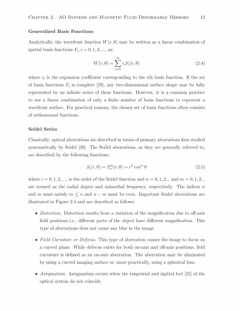
Seidel Series
Classically, optical aberrations are described in terms of primary aberrations first studied
systematically by Seidel [30]. The Seidel aberrations, as they are generally referred to,
are described by the following functions:
Si(r, θ) = Smn (r, θ) = rn cosm θ (2.5)
where i = 0, 1, 2, ..., is the order of the Seidel function and n = 0, 1, 2... and m = 0, 1, 2...
are termed as the radial degree and azimuthal frequency, respectively. The indices n
and m must satisfy m ≤ n and n −m must be even. Important Seidel aberrations are
illustrated in Figure 2.4 and are described as follows:
• Distortion. Distortion results from a variation of the magnification due to off-axis
field positions i.e., different parts of the object have different magnification. This
type of aberrations does not cause any blur in the image.
• Field Curvature or Defocus. This type of aberration causes the image to focus on
a curved plane. While defocus exists for both on-axis and off-axis positions, field
curvature is defined as an on-axis aberration. The aberration may be eliminated
by using a curved imaging surface or, more practically, using a spherical lens.
• Astigmatism. Astigmatism occurs when the tangential and sigittal foci [25] of the
optical system do not coincide.

Chapter 2. AO Systems and Magnetic Fluid Deformable Mirrors 13
−10
1
−10
1−1
0
1
(a) Distortion
−10
1
−10
10
0.5
1
(b) Field curvature
−10
1
−10
10
0.5
1
(c) Astigmatism
−1 0 1−101
−1
−0.5
0
0.5
1
(d) Coma
−10
1
−10
10
0.5
1
(e) Primary spherical aber-
ration
Figure 2.4: Seidel aberrations
• Coma. When rays entering different off-axis parts of the pupil focus at different
points, the result is called coma. Coma causes a tear like image for a point object.
• Spherical Aberrations. Spherical aberration occurs when rays from periphery of the
pupil focus at a point different from the axis.
Zernike Polynomials
The Zernike polynomials have been accepted in vision science as the standard for report-
ing of ocular aberrations [31]. The wavefront function W (r, θ) of a wave with a pupil
radius R can be expressed fully in terms of Zernike polynomials Zi(ρ, θ) as:
W (r, θ) = W (Rρ, θ) =
∞∑
i=0
ciZi(ρ, θ) (2.6)
where ρ = r/R is the normalized pupil radius, and ci is the ith Zernike coefficient. The
Zernike polynomials Zi(ρ, θ) can be written as [32]:
Zi(ρ, θ) = Zmn (ρ, θ) = R|m|
n (ρ)Θm(θ) (2.7)

Chapter 2. AO Systems and Magnetic Fluid Deformable Mirrors 14
where n = 0, 1, 2, ..., andm = 0,±1,±2, ..., are the radial degree and azimuthal frequency,
respectively. The indices n and m must satisfy m ≤ n and n − m must be even. The
radial polynomials R|m|n (ρ) are defined as:
R|m|n (ρ) =
√n + 1
(n−|m|)/2∑
s=0
(−1)s(n− s)!ρn−2s
s![(n +m)/2 − s]![(n−m)/2 − s]!(2.8)
and the triangular functions are defined as
Θm(θ) =
√2 cos |m| θ (m > 0)
1 (m = 0)√
2 sin |m| θ (m < 0)
(2.9)
Figure 2.5 shows the wavefront shapes represented by the first ten Zernike polynomials.
2.1.4 Optical Metrics of Aberrations
In the following, the important question of how different wavefront aberrations affect the
performance of an imaging system is addressed. There are various methods that can be
used to express the effect of a known wavefront aberration on the quality of the resulting
image. Some of these methods are based on the wavefront function W (r, θ) as measured
in the pupil plane, while other methods are based on calculations done in the image plane
[32].
Pupil Plane Metrics
The wavefront aberrations can be most conveniently measured in the exit pupil plane
using a wavefront sensor or an aberrometer which samples the wavefront at discrete loca-
tions in the pupil. The discrete measurements can be used to interpolate the wavefront
anywhere in the pupil by fitting the data using any of the series of basis functions dis-
cussed earlier. When the wavefront function W (r, θ) is represented by one of these series
of basis functions, the diameter of the pupil and the coefficients of the basis functions
are the only quantities required to fully express the aberrations.
• Root Mean Square Error. The most commonly used performance metric in the
pupil plane is the root-mean-square (RMS) of the wavefront function W (r, θ). If
the piston term (i.e. Z00) is ignored, the RMS is the same as the standard deviation

Chapter 2. AO Systems and Magnetic Fluid Deformable Mirrors 15
−10
1
−10
10
1
2
Z00
(a) piston
−10
1
−10
1−1
0
1
Z−11
(b) y-tilt
−10
1
−10
1−1
0
1
Z11
(c) x-tilt
−10
1
−10
1−1
0
1
Z−22
(d) y-astigmatism
−10
1
−10
1−1
0
1
Z02
(e) defocus
−10
1
−10
1−1
0
1
Z22
(f) x-astigmatism
−10
1
−10
1−1
0
1
Z−33
(g) y-trefoil
−10
1
−10
1−1
0
1
Z−13
(h) y-coma
−10
1
−10
1−1
0
1
Z13
(i) x-coma
−10
1
−10
1−1
0
1
Z33
(j) x-trefoil
Figure 2.5: Zernike polynomials.

Chapter 2. AO Systems and Magnetic Fluid Deformable Mirrors 16
of the wavefront function W (r, θ). When the wavefront function W (r, θ) is decom-
posed into Zernike polynomials, the RMS of the function can be measured in terms
of the coefficients ci as
σ =
√√√√
J∑
i=1
c2i (2.10)
where ci is the coefficient of the ith Zernike polynomial and J is the total number
of Zernike polynomials considered for the reconstruction of the wavefront. Similar
expressions can be found for the other basis function series types mentioned above.
• Wavefront Refraction. This is an approximate measure of wavefront error and
considers low order aberrations only. Wavefront refraction can be simply defined
as the radial curvature of aberration, the details of which can be found in [32].
Image Plane Metrics
Though hard to measure directly, the image plane metrics offer a more detailed prediction
of the performance of an imaging system. The following are the most commonly used
metrics which are defined in the image plane:
• Point Spread Function. The point spread function (PSF) describes the response of
an imaging system to a point source or a point object. It can be expressed in terms
of the distribution of the irradiance3 that results from a single point source in the
object space. As shown in Figure 2.6(a), for a diffraction-limited optical system,
the PSF can be visualized simply as the diameter of the Airy disk pattern which
is the resulting image of a point source. The PSF of a typically aberrated system
is shown in 2.6(b). Sometimes, it is more convenient to represent the PSF as a
two-dimensional cross-sectional plot of the irradiance distribution function. Figure
2.7 shows the cross-sectional view the PSF of a typically aberrated wavefront versus
that of a diffraction limited wavefront.
Analytically, the PSF of an optical system can be computed using Fraunhofer
approximation as follows [28]:
PSF (r, θ) = K. |F (P (r, θ))|2 (2.11)
where F (.) represents the Fourier transform operator and K is a constant.
3Irradiance is the power of electromagnetic radiation at a surface, per unit area of the surface [28].

Chapter 2. AO Systems and Magnetic Fluid Deformable Mirrors 17
arc second
arc
seco
nd
−500 0 500
−500
0
500
(a)
arc second
arc
seco
nd
−500 0 500
−500
0
500
(b)
Figure 2.6: Point spread function of (a) diffraction limited wavefront vs. (b) typically
aberrated wavefront.
• Strehl Ratio. It is defined as the ratio of the maximum irradiance of an optical
system over that of a diffraction limited optical system with the same pupil size
and can be written as
S =imaxImax
(2.12)
where imax is the maximum irradiance of the optical system and Imax is the max-
imum irradiance of a diffraction-limited optical system with the same pupil size.
Strehl ratio can also be expressed as the ratio of maximum PSF value of an aber-
rated system to that of a diffraction-limited system as shown in Figure 2.7. How-
ever, this description makes sense only if the PSF of the aberrated system is not too
badly distorted. The higher the Strehl ratio the better is the quality of image. The
best image quality is provided by a diffraction-limited system which has a Strehl
ratio of unity.
• Full Width at Half Maximum. The full width at half maximum (FWHM) intensity
of the PSF of an optical system is another measure of its performance. The metric
is illustrated in Figure 2.7. Generally, the smaller the FWHM, the better is the
quality of the resulting image.
• Optical and Modulation Transfer Functions. These are measures of how much
information is preserved, or modulated, from the object space into the image space.

Chapter 2. AO Systems and Magnetic Fluid Deformable Mirrors 18
tuvwtuvwx yzy |~
~|~ ~~|maxI
maxi
Figure 2.7: Illustration of a 2D point spread function, Strehl ratio and full-width-at-half-
maximum (FWHM).
0 20 40 60 80 100 120 140 160 180 2000
0.1
0.2
0.3
0.4
0.5
0.6
0.7
0.8
0.9
1
cycles/degree
mod
ulat
ion
AberratedDiffraction−limited
0 20 40 60 80 100 120 140 160 180 2000
0.1
0.2
0.3
0.4
0.5
0.6
0.7
0.8
0.9
1
cycles/degree
mod
ulat
ion
AberratedDiffraction−limited
Figure 2.8: Illustration of the modulation transfer function of a diffraction limited wave-
front compared to a typically aberrated wavefront. (a) Vertical. (b) Horizontal.
Analytically, the Optical Transfer Function (OTF) of an imaging system can be
computed using the Fourier transform of its PSF, the details of which can be found
in [28]. The Modulation transfer function (MTF) is the modulus of the OTF.
For illustration purposes, MTF computed on the same point spread functions as
presented in Figure 2.6 is shown in Figure 2.8.
Order of Aberrations
The simple aberrations such as defocus and astigmatism are categorized as the low order
aberrations while the more complex ones are known as high order aberrations. The exact

Chapter 2. AO Systems and Magnetic Fluid Deformable Mirrors 19
definition of the order of aberrations depends on the series of basis functions selected to
describe the wavefront.
The low order aberrations are the main contributors to the overall loss of vision or,
in the case of imaging systems, to the degradation of the quality of images provided by
the systems. Though to a lesser extent, spherical aberrations, coma, and other higher
order aberrations also contribute significantly to the loss of vision or image quality.
In conventional optical systems, the low order aberrations remain the major focus of
the corrective actions taken to improve the vision or image quality. Due to relatively
fewer performance benefits and higher complexity, correction of higher order aberrations
has been limited only to advanced applications, for example, in astronomy. However,
with the significant developments in the imaging technology and the associated systems,
the correction of higher order aberrations has now become a viable - in many cases a
necessary - feature.
2.1.5 Wavefront Correction
Having explained what a wavefront is, how it can be represented and how it can be
used to measure the quality of an imaging system, we now turn to how the wavefront
aberrations can be corrected and how the correction enhances the quality of the aberrated
images. Central to the idea of wavefront correction is the concept of phase conjugation
as explained below [32].
Phase Conjugation
The complex conjugate of the complex amplitude function P (r, θ) = A(r, θ)eiϕ(r,θ), as
given in (2.1) where r represents position (r, θ), is A(r, θ)e−iϕ(r,θ). Analytically, if we
multiply the complex amplitude function A(r, θ)eiϕ(r,θ) with the phase component of its
complex conjugate (i.e., with e−iϕ(r,θ)), the phase of the complex amplitude function is
canceled out. Since the phase of the complex amplitude function represents the optical
aberrations in the system, the multiplication operation amounts to the cancellation of
the aberrations, which is the primary concern of the adaptive optics systems.
The concept is physically implemented by adding, to the original aberrated wave, an
optical aberration which has an equal but opposite phase, as illustrated in Figure 2.9. For
a plane wave propagating towards a flat mirror as shown in Figure 2.9(a), the reflected
wavefront is the same as the incident wavefront. In this configuration, the mirror does not

Chapter 2. AO Systems and Magnetic Fluid Deformable Mirrors 20
(a)
(b)
(c)
(d)
Figure 2.9: Phase conjugation. Effect of (a) flat mirror on plane wave, (b) flat mirror
on aberrated wave, (c) deformed mirror on aberrated wave and (d) refractive medium on
aberrated wave. The dotted lines in (a) to (c) represent the reflected wavefront.
affect the phase of the wave but only reverses the direction of propagation. Similarly, an
aberrated wavefront becomes inverted due to the reflection from the mirror but otherwise
maintains the same shape, as is shown in Figure 2.9(b). However, when the flat mirror
is replaced by a deformed mirror with a deformation half the magnitude of the incident
wavefront, the reflected wavefront becomes flat (Figure 2.9(c)). A similar effect can be
obtained by allowing the aberrated wavefront to pass through a refractive medium which
introduces a wavefront aberration with the same phase but opposite sign as that of the
incident wavefront (2.9(d)).
As described earlier, the aberrations in the wavefront result in an aberrated image.
Therefore, the possibility of canceling out the aberrations in the wavefront using the
principle of phase conjugation provides a direct means of improving the quality of im-
ages provided by an imaging system. The systems that utilize the concept of phase

Chapter 2. AO Systems and Magnetic Fluid Deformable Mirrors 21
conjugation to compensate for the aberrations are called adaptive optics systems. The
idea of phase conjugation is not new and has been used for centuries in the form of
spectacles. The low order aberrations in imaging systems are routinely compensated for
using conventional optical devices such as lenses and mirrors - a manifestation of phase
conjugation. However, the conventional optics do not have the capability to provide the
necessary correction for the higher order aberrations. The AO systems, on the other
hand, provide the ability of compensating for the high order aberrations. Moreover, the
conventional optics are static systems that provide correction for a fixed amount of aber-
rations; the AO systems are designed to provide necessary correction for the dynamically
varying aberrations.
2.1.6 Brief History of Adaptive Optics Systems
The idea of compensating for the high-order aberrations using adaptive optics systems
was first introduced in astronomy by Babcock [7] who proposed that the problem of
astronomical seeing 4 could be solved by incorporating a mirror that provided the possi-
bility of controlling the wavefront shape of the light waves collected for imaging distant
astral bodies. Interestingly, the type of wavefront corrector proposed by Babcock was a
liquid mirror formed by depositing a thin film of oil on the surface of a mirror. Though
this wavefront corrector called Eidophor controlled the wavefront shape by changing the
refractive properties of the film and hence was better comparable to the modern day
spatial light modulators, it is remarkable that the first proposed AO system was based
on the concept of liquid mirrors. Babcock’s idea was not directly put into practice but
it still remains the first published work on adaptive optics systems.
The works of [34] and [35] are considered to be seminal in defining the spatial and
temporal requirements of the AO systems. It was only in 1977 that the first AO system
was realized for an astronomical application [36]. While the bulk of the research work
published since then remains focused on applications in astronomy, a parallel stream of
research has been going on in the field of high energy lasers (HEL) intended for defense
applications. The AO systems used in HEL were aimed at reducing the effects of the
atmospheric turbulence on the laser energy directed at long range strategic targets. Due
to the nature of the HEL applications, a lot of research effort in this area has gone
4Seeing refers to the effects resulting from passage of light rays through the turbulent atmosphere ofthe earth

Chapter 2. AO Systems and Magnetic Fluid Deformable Mirrors 22
into the concept of guide star5 [37, 38]. In early 1990s, a large part of the research
work conducted in the defense sector was made public [4]. The availability of this work
triggered a surge in the astronomical applications of the AO systems. Almost all major
astronomical telescopes were either retrofitted with AO systems or were provided with
integrated AO systems in their design [39, 40]. As the technology matured, it found
applications in other areas such as deep space communications and retinal imaging.
2.1.7 Operating Principle of an Adaptive Optics System
The basic set-up of a typical AO system is shown in Figure 2.10. The main components of
the system include a wavefront sensor, a wavefront corrector - usually a deformable mir-
ror (DM) - and a controller. As shown in the figure, the aberrated light from the source
or the object to be imaged is collected and is directed to the wavefront sensor via the
wavefront corrector. The wavefront sensor measures the deformations in the wavefront
of the incident light. The wavefront deformation information is fed to a control system.
The control system analyses the information and computes the necessary actuator com-
mands . When these commands are applied to the wavefront corrector, the wavefront
corrector adjusts the shape of the mirror surface to cancel out the aberrations in the
incident wavefront. Normally the process of measurement of wavefronts and application
of commands to the wavefront corrector is iterative in nature. When a specified degree
of correction has been achieved, the imaging system is activated to obtain images with
enhanced quality.
In what follows, a brief description of the three basic components of an AO system is
presented. This section also serves as a review of the current state of the art in the AO
technology.
Wavefront Sensors
Over the years, various wavefront sensing technologies such as interferometric sensors,
curvature sensors and Shack-Hartman wavefront sensors have been used [5, 33]. These
wavefront sensors are described in the following:
• Interferometric Wavefront Sensors. This type of wavefront sensors works on the
principle of interferometry. The wavefront measurement data is given in the form
5A guide star is a source of light which can be used as a reference for measurement of the aberrationsto be corrected using an adaptive optics system.

Chapter 2. AO Systems and Magnetic Fluid Deformable Mirrors 23
Figure 2.10: A typical adaptive optics system.
of an interferogram generated by the interference of two wavefronts: a reference
wavefront and the wavefront to be measured. The shape and the magnitude of the
latter is determined by reading the fringe pattern resulting from the interference of
the two wavefronts. A description of the various types of interferometric wavefront
sensors can be found in [33].
• Wavefront Curvature Sensors. A wavefront curvature sensor uses an array of small
lenslets to focus the wavefront into an array of spots. The local phase curvature of
the wavefront is determined by measuring the relative intensities at two different
places along the axis of the beam - one before the focal plane and the other after
the focal plane. The curvature information is then utilized to obtain the wavefront
shape.
• Shack-Hartmann Wavefront Sensors. Recently, Shack-Hartmann wavefront sen-
sor (SHWS) has emerged as the most commonly used type of wavefront sensors,
particularly in vision science. This device samples the wavefront through an ar-
ray of tiny lenslets. Each lenslet creates a focused spot, which is captured by a
CCD camera. The array of spots, when sampling a planar wavefront, would form
a uniform grid pattern as shown in Figure 2.11(a). On the other hand, if the
wavefront is aberrated, the spots will not focus on-axis in the focal plane of their
corresponding lenslets but will deviate according to the local slope of the wavefront
as illustrated in Figure 2.11(b). The displacement of the spots from their on-axis
position measures the local slope of the wave. Using this displacement data, the
complete wavefront shape can be reconstructed. Generally, the data is fit on one

Chapter 2. AO Systems and Magnetic Fluid Deformable Mirrors 24 ¡¢£¤ ¥¦¤ §¢¢¨ ©©ª§¢¢¨ «¬£¤ ¬¤¤¢ £¤ ©©ª ¢¢¨(a) Perfect wavefront®¯°±±²³°´µ²¶°·±¸¹³ º°¹»¼°³®±±²½ ¾¾¿ ®±±²½ ÀÁ¸³ Á²³³°±¹ ¸¹³Â° ¾¾¿ ²±±²½
(b) Aberrated wavefront
Figure 2.11: Working principle of a Shack-Hartmann wavefront sensor.
of the series of two-dimensional spatial functions as described in section 2.1.3. A
detailed description of how the SHWS data is used to reconstruct wavefront shape
is given in Appendix D.
Wavefront Correctors
A wavefront corrector is the principal component of an AO system, which works on the
incident aberrated wavefront and cancels out the aberrations. There are two basic types
of wavefront correctors:
• Spatial Light Modulators. This type of wavefront correctors uses arrays of liquid
crystal micro-lenses [41, 42]. The phase of the light passing through the array can
be controlled by electronically or optically manipulating the refractive index of the
individual micro-lenses. The phase modulation provides the necessary means to
control the wavefront shape. The spatial light modulators (SLMs) are available in
both reflective as well as transparent modes. This type of wavefront correctors has
the advantage of very high spatial resolution provided by the extremely small liquid
crystals. Since they are based on the existing LCD technology, they also have a

Chapter 2. AO Systems and Magnetic Fluid Deformable Mirrors 25
significant cost advantage over the other types of wavefront correctors. SLMs are
limited by a small stroke or magnitude of correction that they can provide. Another
limitation is the requirement of linearly polarized light since the liquid crystals can
modulate only the light polarized along their axis.
• Deformable Mirrors. Deformable mirrors (DM) have evolved as the most widely
used wavefront correction elements in adaptive optics systems. These mirrors are
characterized by a reflective surface which can be locally deformed hence providing
a means to change the wavefront shape of the reflected light. The main advantage
of these mirrors is their reflective nature that allows for a low loss of radiant energy
and hence makes them particularly suitable for applications where the intensity of
light is, or needs to be, low.
Based on the type of reflective surface, DMs may be classified as segmented or
continuous type.
1. Segmented mirrors feature an array of mirror segments each of which can be
individually controlled [43, 44, 45]. Figure 2.12 shows a typical segmented mir-
ror. Some of these devices are piston only where each segment can be moved
perpendicular to the mirror plane typically using a single actuator. Others
can be tipped and tilted, and are generally supported by three actuators per
segment. Thanks to the micro-machining technology, these mirrors can be
fabricated with a very high density of segments. For example, Boston Mi-
cromachines offers segmented mirrors with 140 segments in 4.9 mm diameter
aperture. However, the segmented mirrors reported thus far have relatively
small stroke lengths; 5.5 µm for the Boston Micromachines mirror mentioned
above. Also, these mirrors are known to have better operating speeds. The
percentage of the surface area of a segmented mirror covered by reflective seg-
ments is known as the fill factor. The segmented mirrors with low fill factor are
not preferred due to the loss of energy at the discontinuities in their surface.
The segments can be square or hexagonal in shape. As each segment can be
adjusted independently, these mirrors are considered to be more suitable for
correcting wavefront aberrations with higher spatial frequencies [65].
2. Continuous mirrors are characterized by a flexible, continuous reflecting sur-
face which can be locally deformed using an appropriate actuation mechanism

Chapter 2. AO Systems and Magnetic Fluid Deformable Mirrors 26
Figure 2.12: Schematic of a segmented deformable mirror.
Figure 2.13: Types of continuous surface mirrors.
[46, 47, 48, 49]. Typically when an actuator in a continuous DM is activated,
the surface deflection is not restricted to the area directly above that actuator
but extends to the neighboring actuators. This phenomenon is called actuator
coupling. The continuous mirrors remain the wavefront corrector of choice for
many applications because of the low loss of energy. Based on the actuation
mechanism, these mirrors may be further categorized into four types as shown
in Figure 2.13.
– Figure 2.13(a) shows a type of continuous surface deformable mirrors
which utilizes actuators that expand when a voltage is applied. Examples
of this type or mirrors are a 97-actuator mirror from Xinetics Inc. [52]

Chapter 2. AO Systems and Magnetic Fluid Deformable Mirrors 27
and a 37-actuator mirror from OKO Technologies [53].
– Bimorph mirrors consist of layers of dissimilar materials as shown in Fig-
ure 2.13(b). By controlling the voltage applied to an electrode, the curva-
ture of the mirror surface can be changed, which serves the purpose of a
deformable mirror. A 35-actuator mirror with 15 mm diameter produced
by AOptix is the typical example of this category of deformable mirrors
[53].
– Shown in Figure 2.13(c) is an example of the membrane mirrors that
utilize electrostatic attraction to deform the mirror surface coated on a
flexible membrane. OKO Technologies mirror with 37-actuators and 15
mm diameter pupil is an example of this type of mirrors. The membrane
clamped at its edges can provide up to 9 µm of peak-to-valley surface
deflections.
– Figure 2.13(d) shows another membrane type mirror that utilizes electro-
magnetic force between small permanent magnets attached to the mem-
brane and electromagnetic coils placed underneath the magnets. A 52-
actuator mirror with 15 mm diameter pupil offered by Imagine Eyes is an
example of this type of mirrors. The mirrors is reported to have up to 50
µm surface deflections [54].
All these mirror mentioned above have their trade-offs, some of which have been
investigated and reported in studies [12, 52, 53].
Controllers
A controller is the vital link between the wavefront sensor and the wavefront corrector in
an AO system. Its function is to convert the wavefront aberration measurements made by
the wavefront sensor into a set of actuator commands that are applied to the wavefront
corrector to cancel the wavefront aberrations. Since the wavefront correctors act on the
wavefront shape of the incident wave, the wavefront corrector control problem faced in
AO can be generalized as a shape control problem. Within the context of the DMs, the
objective of the shape control is to obtain a shape for the mirror that best tracks the
shape required to cancel the aberrations.

Chapter 2. AO Systems and Magnetic Fluid Deformable Mirrors 28
Control Methods A wide range of controllers for AO systems has been reported in
the literature. The controller used in AO system can be broadly grouped as Proportional-
Integral-Derivative (PID) type controllers, optimal controllers and adaptive controllers.
A brief review of these controllers is presented as follows.
• PID Controllers. Most controllers for AO systems have used proportional-integral-
derivative (PID) feedback of the measured wavefront error above each actuator to
control that actuator [50, 51, 66, 56]. The objective of these systems is to drive the
wavefront error to zero. Traditionally, single-input single-output (SISO) integral or
PID controllers have been developed for a single actuator. The controller is then
duplicated for each actuator.
Most of the controllers used in AO systems are based on DC models the response of
the wavefront correctors used in these systems. The DC models are experimentally
obtained by measuring the wavefront shape resulting from applying a constant in-
put to each of the actuators. The resulting input-output map is usually referred to
as the influence function of the wavefront corrector and is employed to determine
the necessary control input for the wavefront corrector. Traditionally, either pro-
portional or proportional-integral structure is employed to provide updates of the
inputs when using the influence function based controllers [5].
• Optimal Controllers. Optimal controllers employ mathematical optimization meth-
ods to obtain the controller parameters that provide a specified performance ob-
jective such as the minimization of the wavefront shape error. A number of control
algorithms used in AO systems employ Linear-Quadratic-Gaussian (LQG) criterion
which seeks to minimize a quadratic cost function and, thus, determine the con-
troller that minimizes the error between the actual shape and the desired shape of
the wavefront corrector [57, 58, 59, 60].
H2 and H∞ based optimal controllers that seek to optimize the response of the
overall system have also been reported in the literature. [61, 62]
• Adaptive Controllers. Due to the dynamic nature of the aberrations in most of
the applications of AO systems, the shape control problem addressed in AO is the
tracking of an unknown and time-varying shape for the wavefront corrector (i.e.,
desired shape of the mirror). Since the desired shape of the wavefront corrector is
unknown and time-varying, the controller must be tuned online to converge to the

Chapter 2. AO Systems and Magnetic Fluid Deformable Mirrors 29
controller needed to achieve the desired control objective. This type of controllers
whose parameters can be tuned online are called adaptive controllers. They are
a relatively recent addition to the list of controllers used in AO systems but are
expected to dominate the control systems in the future AO applications [63, 64].
Control Architectures Using any of the above mentioned methods, the controller
design can be implemented with one of the three control architectures: centralized, de-
centralized and localized.
• Centralized Control. The centralized control architecture uses all the measurement
data from the sensors to simultaneously compute the control inputs for all of the
actuators of the wavefront corrector. It can achieve the best performance results
but is computationally expensive. Implementation of the centralized controller may
not be feasible for systems with a large number of actuators.
• Decentralized Control. In decentralized controllers, information from a single sensor
is used to generate the control signal for one of the actuators [66]. The decentralized
controllers are easy to implement. However, they have a limited performance as
compared to that obtained using centralized controllers.
• Localized Control. A localized controller uses information from several neighboring
sensors to generate commands to a given actuator [67, 68].
2.2 Retinal Imaging Adaptive Optics Systems
The eye is an imaging system that forms one of the primary faculties of the human sensory
system. It has long been known that the normal human eye suffers from many different
aberrations that affect the vision of the individual. The most common aberrations in the
human eye are defocus and astigmatism. The normal eyes are also known to suffer from
additional aberrations such as spherical aberrations, coma-like aberrations and a host of
irregular aberrations.
The uncorrected aberrations in the eye affect not only what it can see but also de-
termine the smallest internal structures that can be observed when looking into the eye.
The various imaging technologies, which are used to examine the internal parts of the
eye are affected by this phenomenon. Specifically, the naturally existing aberrations in

Chapter 2. AO Systems and Magnetic Fluid Deformable Mirrors 30
the eye degrade the quality of the retinal images obtained by the various available tech-
nologies such as funduscopy, scanning laser ophthalmoscopy (SLO) and optical coherence
tomography (OCT) [65].
Figure 2.14 shows the margin of improvement in the image quality that can be
achieved by correcting higher-order aberrations [134]. Shown in the figure is the best
MTF of the eye averaged over 14 eyes with 3 mm pupil with an optimal correction of
defocus and astigmatism. This represents the best image quality that can be achieved
by rectifying the low-order aberrations only. Now compare it to the ideal MTF of the
eye with an 8 mm pupil blurred only by diffraction, which represents the best image
quality with all the aberrations - including the high-order aberrations - compensated for.
The figure shows that finer spatial details can be observed in a diffraction limited eye
with a dilated pupil as compared to an aberrated eye with a regular pupil size. The
shaded area between the two plots shows the range of image contrasts and spatial fre-
quencies (resolution) that are available for imaging of the retina only if the high-order
aberrations are corrected. This clearly shows the need of a system that can be used to
compensate for the high-order aberrations in the eye and and has been the driving force
behind research efforts made over the years to incorporate AO systems in ophthalmic
imaging systems. Before dwelling on how the AO systems are used to compensate for
the higher-order aberrations in the eye, a quick overview of the sources and the nature
of the ocular aberrations is presented.
2.2.1 The Structure of the Eye
Figure 2.15 shows the anatomy of the human eye. The principle optical components in
the eye are, the cornea, the iris and the lens.
• The Cornea This is the first surface of the eye and is actually an extension of the
white outer shell of the eye. Intermittent closing of the eye lids keeps a tear film
on the front surface of the cornea. Due to a high refractive index (≈ 1.376) and a
small radius of curvature (≈ 7.7 − 6.8 mm), the cornea offers the highest optical
power (≈ 43 diopters)6 among all the parts of the eye.
• The Iris The iris serves the important purpose of regulating the amount of light
6A diopter is a unit of measurement of the optical power of a lens or curved mirror, which is equalto the reciprocal of the focal length measured in meters [25].

Chapter 2. AO Systems and Magnetic Fluid Deformable Mirrors 31
ÃÄÅÆÇÈÉÅ
Figure 2.14: Potential benefit of correcting the higher-order aberrations in the eye
(Adopted from [134]).
Figure 2.15: Structure of the eye.
Chapter 2. AO Systems and Magnetic Fluid Deformable Mirrors 32
that enters the eye. It also alters the numerical aperture (NA) of the eye.
• The Lens Located immediately behind the iris, the lens is the second major con-
tributor to the optical power of the eye adding up to 30 diopters. Contraction and
expansion of the lens provides the critical capability of focusing, or accommodation
as it is termed, to the eye.
• The Retina The retina is the part of the eye where image is formed. The retina
comprises of millions of photoreceptor cells lining the interior wall of the eye. Like
a CCD array in artificial imaging systems, these cells sample the image that is
projected on the retina by the above mentioned optical parts of the eye. The pho-
toreceptor cells are either rod-like or cone-like in shape. The cone photoreceptors
are of three types each providing color vision.
2.2.2 Sources of Aberrations in the Eye
Ideally, the optical parts of the eye should be able to precisely project the image of an
object on the spherical surface of the retina. Conversely, for the case of imaging of the
retina, the light reflected from any point on the retina should exit the eye as a perfect
plane wave. However, none of the propositions is true in actual physical eye. Even the
normal eye with 20/20 vision prescription also suffers from naturally occurring defects
that result in a less than perfect image being formed on the retina. The same is true
when taking an image of the retina itself. The light reflected from an aberrated eye
does not exit as a planar and thus results in a blurred image of the retina. There are a
number of physical and physiological aspects that contribute towards the eye being less
than perfect in its function.
The first source of aberrations in the eye is improper focusing which may arise either
from abnormal changes in the refracting parts e.g., the cornea and the lens, or from
deformation of the eyeball that alters the distance between the lens and the retina. The
latter is the more common of the two, causing roughly 65% of all young adults to require
eyeglass correction.
Since the cornea and the lens provide major share of the refractive power of the eye,
they are also the main source of aberrations in the eye[27]. In the cornea, the main
contribution comes from the outer surface, which has most of the corneal power. While
it is certain that the primary sources of optical power play fundamental role in defining

Chapter 2. AO Systems and Magnetic Fluid Deformable Mirrors 33
the total aberrations in the eye, the relative contribution of different sources remains far
from certain. Contrary to some studies which suggest that lens contributes more to the
total aberrations [70], others have concluded that the lens has a compensatory effect on
the aberrations caused by the cornea [71, 72].
The other major source of aberrations is accommodation which results from a change
in the shape of the lens. Studies have revealed that the change in aberration from accom-
modation is roughly the same magnitude as the total aberration in any accommodation
condition [72]. Since the change in aberrations is high, the lens stands out as the major
contributor of the total aberrations. More importantly, it reveals that the aberrations
are dynamic in nature and any wavefront correction that is applied at any particular
accommodation condition remains optimal for that condition only; any departures from
this condition will cause loss of the benefit achieved from the correction.
Tear film has also been diagnosed as one of the main sources of aberrations in the
eye [73, 74, 75]. The tear film in the human eye is a layer approximately 10 µm thick
made up mostly of water. It offers the first optical surface of the eye. Because of its
large curvature and high refractive index, the tear film contributes significantly towards
the total aberrations in the eye. The liquid nature of the tear film means that due to
the effects of eye movements, and the pressure exerted by the eye lids, this surface is not
static, and hence the aberrations it introduces to are also dynamic in nature[73].
2.2.3 Dynamics of the Aberrations in the Eye
Although aberrations in the human eye have been studied since long, it was only after
the recent introduction of AO systems in ophthalmic imaging systems that the dynamics
of the aberrations became the focus of many studies. The dynamics of the higher-order
aberrations were first characterized by [72]. Prior to this only microfluctuations in focus
had been characterized. They found measurable fluctuations up to around 5−6 Hz. Based
on these results they suggested that an AO system capable of correcting fluctuations of
up to 1 − 2 Hz would be sufficient to yield diffraction limited resolution over a dilated
pupil. In [76], fluctuations as high as 30 Hz were observed with an adaptive optics system
with sampling rates as high as 240 Hz. However, negligible improvement in image quality
was achieved with this system when correcting for aberrations over 10 Hz. These results
suggest that although high frequency fluctuations contribute to the aberrations in the
eye, they have a small effect on retinal image quality. It is estimated that the control

Chapter 2. AO Systems and Magnetic Fluid Deformable Mirrors 34
Figure 2.16: Averaged power spectra for Zernike modes of different orders for a human
subject with paralyzed accommodation (4.7-mm pupil) (Adopted from [72]).
system for an adaptive optics system requires a sampling rate of about 10 times the
highest frequency of the fluctuations in the eye. This implies that an adequate sampling
rate to consider is about 50 Hz to deal with most of the significant fluctuations in the
human eye [72].
The power carried by the fluctuations in the ocular aberrations decreases with in-
creasing spatial order of the aberrations. This can be observed in Figure 2.16 (adapted
from [72]), which shows how the fluctuations of the total wave-front error are distributed
among different Zernike radial orders for one subject with paralyzed accommodation. As
can be observed from the figure, the relative power of different Zernike modes decreases
with the increasing order of the Zernike modes.
There are various sources of variations in the aberrations of the eye. The typical ocu-
lar dynamics that affect the aberrations are accommodation [77, 78], tear film dynamics
[73, 74, 75], and cardiovascular activity [79].
Just as the cornea contributes large static aberrations due to its curvature, the tear
film provides the most powerful optical surface with dynamic aberration content [73].

Chapter 2. AO Systems and Magnetic Fluid Deformable Mirrors 35
The strongest contributions to the tear film aberration changes are due to lower fre-
quency aberrations, typically lower than 2 Hz. However, it has been shown that there
are measurable contributions to the tear film aberration up to 11 Hz [73].
Microfluctuations of accommodation is another possible source of fluctuations in the
wavefront aberrations in the eye. Even at steady viewing conditions, the eye constantly
changes its focus. Support for this comes from evidence that accommodations in the eye’s
focus produce changes in other aberrations. For example, it was shown in [72] that large
voluntary changes in focus of the eye produces systematic changes in spherical aberra-
tions. However, it has also been suggested that microfluctuations in accommodation are
not the primary cause for fluctuations in the other aberrations [73].
Another possible cause for fluctuations in wavefront aberrations is the movement of
the eye. There are at least two kinds of movements in the eye: rotation and translation.
Rotation of the eye is caused by fixational eye movements and is usually very small
for a fixated eye and is unlikely to correspond to significant changes in the wavefront
aberration [72]. Translation is caused by small instabilities in the head position and
because of small changes in fixation. Fluctuations that are due to pupil translation will
not affect a person’s visual performance in ordinary viewing conditions; however, will
reduce the image quality in adaptive optics system used to take high resolution retinal
images. Experimental results obtained in [72] show that neither eye rotation or pupil
translation are a major source of the fluctuations in wavefront aberrations.
2.2.4 Correction of the Aberration in Eye using AO System
It is established that the correction of high-order aberrations in the eye carries significant
visual and image quality benefits. This has been the driving force behind a number
of research efforts undertaken during the last one decade in order to integrate AO in
systems ranging from funduscopes to laser surgery. A brief exposition of the ophthalmic
technologies which have benefited from AO systems is presented in the following.
Retinal Imaging
The most extensively used application of AO in the eye is retinal imaging, which provides
high resolution images of the living retina. The ability to examine in vivo the minute
details of the retinal tissue allows the early detection and regular monitoring of retinal
diseases. There are three main imaging modalities which have thus far been utilizing AO

Chapter 2. AO Systems and Magnetic Fluid Deformable Mirrors 36
systems [65].
• Flood Illumination Ophthalmoscopy. This is the most commonly used and straight
forward imaging technique that combines AO with direct imaging of the retina.
It employs a low coherence7 source of light which illuminates a localized patch of
retina. A CCD camera placed in conjugation with the retinal plane is used to
collect the light reflected from the retina and take the image of the illuminated
patch.
Figure 2.17 shows the layout of a basic retinal imaging system augmented with AO.
A light beam with a planar wavefront originating from a light source - usually a laser
or a super-luminescent diode (SLD) - is directed to the retina of the eye. The light
reflects from the retina and exits the eye as a beam having an aberrated wavefront
- the aberrations being induced by the sources mentioned earlier. The beam is
directed to the DM and the reflection from the mirror is detected by the wavefront
sensor. The wavefront sensor measures the magnitude of the aberrations over the
whole pupil. The measurements are fed to a control system which computes the
appropriate command signals for the DM. The signals, when applied to the DM,
deform the shape of the mirror surface such that the aberrations in the wavefront
of incident beam are iteratively canceled out. When a desired level of cancellation
or correction is achieved, an illumination source such as a flash lamp is turned on.
The light from this source floods the retina of the eye and is reflected back following
the same path as that of the the laser/SLD light. A dichroic mirror 8 reflects the
light to the imaging system which collects the image of the retina. Note that the
flood light reflected from the retina still carries the aberration as it exits the eye.
Before reaching the camera, however, the aberrations are canceled out by the DM
which now is appropriately deformed to do so.
• Scanning Laser Ophthalmoscopy. It may be noted that the ophthalmoscope de-
scribed above provides no depth resolution on the retinal tissue and AO augmen-
tation enhances only the transverse resolution of the images. Scanning laser oph-
thalmoscopy (SLO), on the other hand, is an imaging technique which also offers
7Coherence is a property of waves, that enables stationary (i.e. temporally and spatially constant)interference. Two waves are said to be coherent if they have a constant relative phase, which also impliesthat they have the same frequency.
8A dichroic mirror reflects a certain range of wavelengths (colors) of the light while allowing theremaining wavelengths to pass through.

Chapter 2. AO Systems and Magnetic Fluid Deformable Mirrors 37
Figure 2.17: A typical retinal imaging adaptive optics system.
axial resolution i.e., the layers beneath the surface of the photoreceptor cells can be
distinctly imaged. SLO utilizes a laser beam which is scanned across the retina and
the image is built-up point by point. As shown in Figure 2.18, the reflected light is
made to pass through a small aperture called confocal pin-hole, which is placed in
conjugation with the retinal plane. This arrangement increases the contrast level
of focused axial location by preventing the light reflected from other layers of the
retinal tissue and hence offers the desired depth resolution. Sensing the wavefront
of the same light as used for the basic SLO, a wavefront corrector can be inserted
into the optical system such that the wavefront aberrations introduced by the eye
are canceled out before the reflected laser light passes through the pin-hole and is
detected by the image detector.
• Optical Coherence Tomography. This is another imaging method which provides
both transverse and axial resolution of retinal images, mostly performing better
than SLO. It is based on interferometric principle and uses a Michelson interferom-
eter in conjunction with a low coherence light source [80]. OCT systems have been
devised in two different types: time-domain OCT and spectral OCT.

Chapter 2. AO Systems and Magnetic Fluid Deformable Mirrors 38ÊËÌÍÍÎÍÏ ÐÑÒÎËÓ ÌÍÔÕÔÌÑÒÎÖ× ÐÑÒÎËÓØÙÌÍ× ÚÛ ÛÚËÜÓ ÝÚÍÛÚËÌÙØÎÍÞÚÙ×ß×Ò×ËÒÚàáÌÓ×à
Figure 2.18: The working principle of a scanning laser ophthalmoscope.
2.2.5 History of Ophthalmic Adaptive Optics Systems
Shortly after Babcock [7] introduced the concept of AO in astronomy, Smirnov [117]
suggested the idea of correcting the high-order aberrations in the eye, probably indepen-
dently from the existing ideas in astronomy. However, it was not until late 1980s that this
idea could be put into practice. Dreher et. al. [8] were the first to use a deformable mir-
ror to improve the quality of images provided by scanning laser ophthalmoscope, though
they corrected static astigmatism only. Artal and Navarro [118] achieved measurement of
inter-center distance between photoreceptor cones using speckle interferometry, a method
well-known in astronomy. Miller et. al. [119] were the first to obtain direct images of the
retina using a high-resolution fundus camera. Though they corrected defocus and astig-
matism only, they were able to obtain up to 3.5 µm resolution. The real breakthrough
came when Liang [120] demonstrated that the Shack-Hartman wavefront sensor could be
used to measure the ocular aberrations. This prompted a number of studies that sought
to provide wavefront correction promising diffraction-limited images of the retina.
In 1997, Liang et al. [134] incorporated the Shack-Hartman wavefront sensor in an
AO system and obtained images with unprecedented high resolution. By correcting
the higher-order aberrations, they were able to obtain images with enough photometric
accuracy to identify microscopic structures as small as the single cone cell. They reported
up to 3.2-fold improvement in the transverse resolution over that of a 2.5 mm pupil.
Significant enhancements in the contrast sensitivity of the eye were also reported.
Hofer et al [72] were the first to study and correct temporal variations in the ocular
aberrations using closed-loop AO systems. They reported three-fold improvements in

Chapter 2. AO Systems and Magnetic Fluid Deformable Mirrors 39
Strehl ratio and up to 33% increase in contrast of the images of the cone photorecep-
tors. They reported dynamic compensation of up to 5th order Zernike polynomials with
frequency up to 0.8 Hz.
The new-found capability of measuring and correcting the high-order aberrations in
the eye has facilitated developments such as identification of the arrangement of the three
classes of photoreceptor cells [9], psychological testing of the functioning of vision at the
neural level [10], and finding of alternate causes of color blindness [11].
Beside direct retinal imaging, OCT and SLO too have benefited from AO. Optical
coherence tomography remains one of the most promising applications of AO systems
[80]. Moreover, when incorporated into a scanning laser ophthalmoscope (SLO), AO
systems have significantly improved the lateral resolution of this type of ophthalmoscopy
[81].
2.2.6 Challenges to Ophthalmic Adaptive Optics Systems
Despite the demonstrated potential of the ophthalmic AO systems, the use of these
systems has been limited only to research studies and they are still not available for the
clinical imaging applications. Some of the relevant problems impeding the widespread
accessibility of these systems are as follows:
• High Stroke Requirement. A set of generalized requirements for ophthalmic appli-
cations of wavefront correctors is presented in [13]. One of the most significant
requirements of the wavefront correctors is the unusually high stroke needed to
compensate for the large magnitude (peak-to-valley path length difference) of the
wavefront aberrations in the eye. For a deformable mirror with the proposed size of
10 mm diameter, [12] suggest a minimum of ±12µm of surface deflection as needed
to compensate for the typical aberrations in the eye. For specific applications, [13]
report a requirement of deformable mirror strokes as high as 53µm. A survey of the
wavefront correctors being used in ophthalmic AO systems is also presented in [13].
None of the surveyed wavefront correctors meets the requirements of ophthalmic
AO systems as mentioned above. Only recently magnetic deformable mirrors with
sufficient stroke have been reported [54].
Currently, a number of strategies are being used to work around the requirement
of a large stroke. Some of these strategies include use of optical components, such
as Badal optometer [82] and Alvarez lens pairs [83], to separately compensate the

Chapter 2. AO Systems and Magnetic Fluid Deformable Mirrors 40
low-order aberrations, cascading of two deformable mirrors [84, 85], and double
incidence of the aberrated wave on the deformable mirror [86]. All these strategies
add to the complexity, size and cost of the AO system. Therefore, a wavefront
corrector that could provide a large peak-to-valley wavefront correction is needed.
• Hight cost of the current AO systems is another major impediment to the widespread
accessibility of these systems in ophthalmic imaging systems. For wavefront correc-
tors to be available for the routine ophthalmic imaging, [12] suggest an average cost
of $10 per actuator. Currently, the cost of a wavefront corrector ranges between
$100-$1000 per actuator. Therefore, only a significant cost reduction will render
these systems viable for applications in ophthalmic imaging systems.
2.3 Magnetic Fluid Deformable Mirrors
Magnetic fluid deformable mirrors (MFDMs) were proposed a few years ago as an al-
ternative to the conventional wavefront correctors in AO systems [14]. Though the idea
of these mirrors is quite recent, they have been appraised by a number of preliminary
studies [17, 15] as a promising future technology. This section presents a brief review of
their composition and operating principle. Important properties of the magnetic fluids
and MELLFs - the key constituents of a MFDM - are briefly described. The known
advantages, limitations and potential applications of this new type of deformable mirrors
are also discussed.
2.3.1 Principle of Operation
The free surface of a liquid follows an equipotential surface9 to a very high degree of
precision. This characteristic of liquids can be exploited to deform their surface to any
desired shape. The process of shaping the free surface may be controlled by varying one
or more of the force fields that contribute toward the potential level. Magnetic fluids are
a class of liquids which respond to variations in magnetic field and hence their surface
shape can be controlled by controlling the magnetic field that they are exposed to. If a
beam of light incident on the free surface of a magnetic fluid can be adequately reflected,
9Equipotential surfaces are surfaces of constant scalar potential, which is the total energy associatedwith all the conservative forces acting on a system.
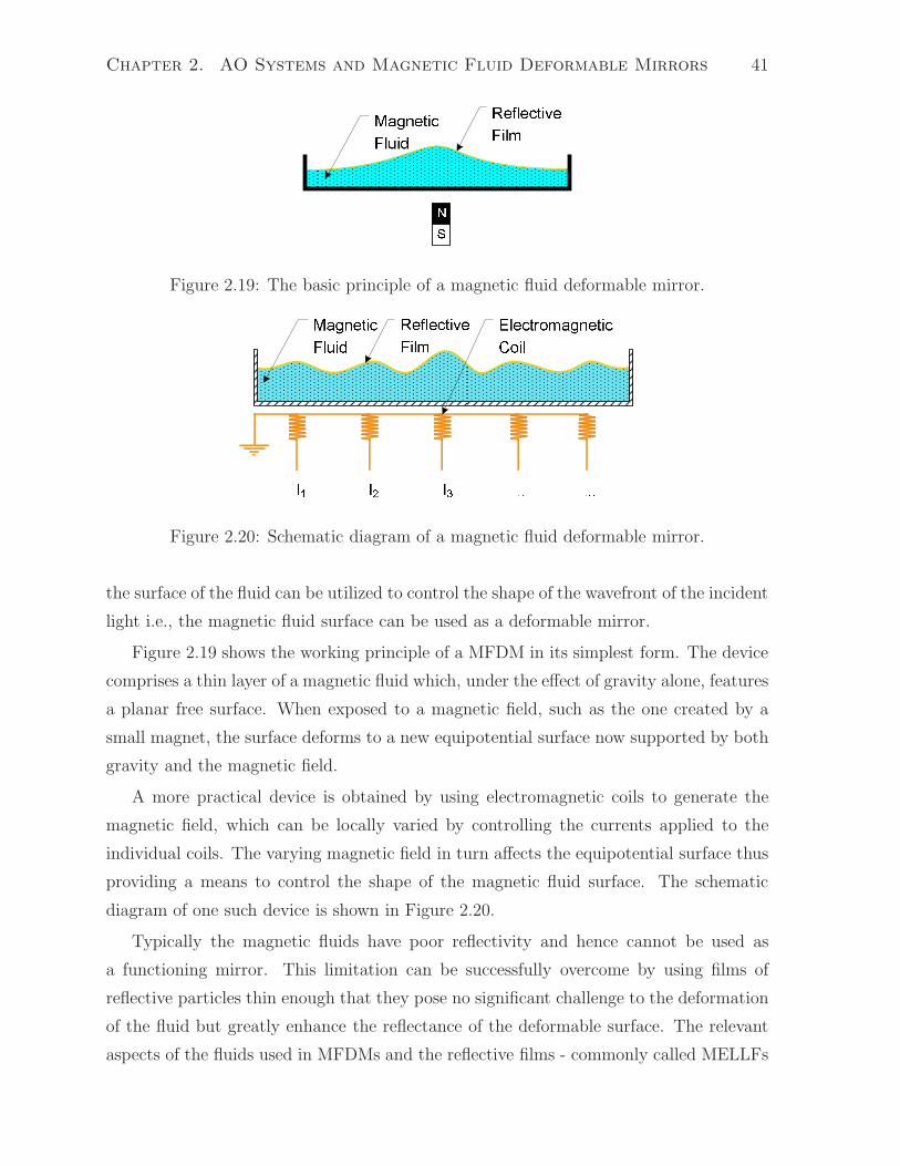
Chapter 2. AO Systems and Magnetic Fluid Deformable Mirrors 41
Figure 2.19: The basic principle of a magnetic fluid deformable mirror.
Figure 2.20: Schematic diagram of a magnetic fluid deformable mirror.
the surface of the fluid can be utilized to control the shape of the wavefront of the incident
light i.e., the magnetic fluid surface can be used as a deformable mirror.
Figure 2.19 shows the working principle of a MFDM in its simplest form. The device
comprises a thin layer of a magnetic fluid which, under the effect of gravity alone, features
a planar free surface. When exposed to a magnetic field, such as the one created by a
small magnet, the surface deforms to a new equipotential surface now supported by both
gravity and the magnetic field.
A more practical device is obtained by using electromagnetic coils to generate the
magnetic field, which can be locally varied by controlling the currents applied to the
individual coils. The varying magnetic field in turn affects the equipotential surface thus
providing a means to control the shape of the magnetic fluid surface. The schematic
diagram of one such device is shown in Figure 2.20.
Typically the magnetic fluids have poor reflectivity and hence cannot be used as
a functioning mirror. This limitation can be successfully overcome by using films of
reflective particles thin enough that they pose no significant challenge to the deformation
of the fluid but greatly enhance the reflectance of the deformable surface. The relevant
aspects of the fluids used in MFDMs and the reflective films - commonly called MELLFs

Chapter 2. AO Systems and Magnetic Fluid Deformable Mirrors 42
- are described in the following paragraphs.
2.3.2 Brief History of Development of MFDMs
The idea of using a liquid mirror is more than a century old [87]. However, it was only
in late 1980s that the concept was put into practical use. The exceptionally good surface
qualities of liquids led NASA to use Liquid Mirror Telescopes (LMTs) for astronomical
applications [88, 89, 90].
The success of LMTs led to the idea of deforming liquid mirrors to obtain mirror
shapes other than a parabola. Shutter and Whitehead [91] proposed to use magnets
to re-shape the classical mercury-based parabolic mirror into a sphere. They used an
amalgam of iron and mercury to influence the liquid bulk by applying a magnetic field.
Ragazzoni and Marchetti [92] proposed the first adaptive liquid mirror that used an
electrically conducting metallic reflective liquid that could carry a current and was shaped
by a number of current carrying coils. All these earlier attempts including the LMTs
revolved around mercury which has excellent reflective properties. However, mercury
suffers from serious limitations when attempted to be deformed electromagnetically. The
high density of mercury necessitates very large electromagnetic force to achieve even
minimum required surface deflections. This requirement of large force means prohibitively
large currents running through the electromagnetic coils used to generate the magnetic
field. Attempts to deform mercury by running currents through the liquid suffered from
yet another drawback i.e., joule heating of the liquid.
Confronted with these limitations of mercury, researchers came up with an innovative
new technology that utilized the concept of magnetic fluid deformation introduced in
section 2.3.1 above. The low density of carrier fluids such as water and oils afforded
a great advantage over mercury since the current requirements for the deformation of
these liquids are orders of magnitude lower than those for mercury. This development
prompted a number of studies that explored the possibility of using the MFDMs in
applications ranging from extremely large LMTs to ophthalmic AO systems. The initial
studies reported thus far show that these mirrors can provide tens of micrometer of
surface deflection [15, 17, 16]. Despite the initial success and promising future prospects,
MFDMs have yet to see a practical application owing mainly to some critical impediments
as discussed in section 2.3.5.

Chapter 2. AO Systems and Magnetic Fluid Deformable Mirrors 43
2.3.3 Magnetic Fluids
Composition
Magnetic fluids - also called ferrofluids - are stable colloidal suspensions of nano-sized,
single-domain ferri- or ferro-magnetic particles. When subjected to a magnetic field, the
suspended particles affect the flow properties of the carrier fluid. As mentioned earlier,
one of these effects is the variation of shape of the fluid free surface, which has been
exploited to develop deformable mirrors.
Depending on the type of the carrier fluid used, the magnetic fluids can be broadly
categorized as water-based and oil-based systems. In most technological applications of
magnetic fluids, the magnetic particles are obtained from one of a number of different
ferrites. By far the most commonly used ferrites are magnetite (Fe3O4) and maghemite
(γ − Fe2O3). The magnetic particles can also be obtained from metals such as iron and
cobalt. The typical size of these particles is 10 nm in diameter.
Since the individual magnetic particles are in a permanent state of saturation magne-
tization, there exists a strong magneto-static attraction between the particles and, as a
result, the particles tend to agglomerate in the carrier fluid. To avoid the agglomeration,
the magnetic particles are coated with surfactants, which introduce an entropic repulsion
between the particles resulting in stable suspensions of the particles. In some applica-
tions, the repulsive mechanism is achieved by charging the surface of the particles, which
produces an electrostatic repulsion.
Properties
There exists a vast selection of fluids which may be utilized as carriers in the magnetic
fluids. Similarly, a considerable degree of freedom may be exercised when choosing the
magnetic particles and surfactant material properties. The choice of materials allows for
a very wide range of properties that can be built into a desired magnetic fluid. Density,
viscosity, surface tension, magnetic permeability and saturation magnetization are some
of the properties of a magnetic fluid that can be varied according to the requirements of
an intended application.
The response of a MFDM depends on the properties of the magnetic fluid selected
for the application. The surface deflection resulting from applying a given magnetic field
is a function of the fluid properties such as density, magnetic permeability and surface
tension.

Chapter 2. AO Systems and Magnetic Fluid Deformable Mirrors 44
Owing to the incompressible nature of the commonly used carrier fluids, most of the
magnetic fluids can be characterized as incompressible. However, when exposed to a high
enough magnetic field, they exhibit a unique behavior showing compression of the bulk
fluid. This phenomenon is called magnetostriction.
When exposed to a uniform, vertical magnetic field, the magnetic fluids show no
response at low magnetic flux densities. However, if the field strength exceeds a certain
value ( 17 mT) [93], a well-known instability results in patterns of spontaneous protrusions
of the free surface of the fluid. This phenomenon is called Rosensweig instability [94].
Synthesis
The magnetic fluids can be synthesized using a number of different methods. The earlier
approach was to grind micro-sized magnetite particles in a ball-mill in the presence of a
surfactant material and a carrier fluid until the particle reaches the desired nano-meter
range size [124]. However, this process usually takes a very long time, and now magnetic
fluids are produced more conveniently by chemical methods involving the co-precipitation
of metal salts in aqueous solution using a base. A typical chemical process employed in
the synthesis of magnetic fluids is as follows:
2Fe3+ + Fe2+ + 8OH− = FeOFe2O3 + 4H2O
Beside the co-precipitation method, numerous other methods can be used to obtain both
ferrite and metal based magnetic fluids [95].
Applications of Magnetic Fluids
Since their introduction in early 1960s, magnetic fluids have seen applications ranging
from sink-float systems to drug delivery systems. Some of the well-known applications
include liquid seals, dampers for audio speakers and heat-transfer agents. They are also
being investigated for applications in MEMS and nano-technology [96, 97]. Of course,
their use as MFDMs, particularly in ophthalmic AO systems, remains one of the most
advanced applications. Beside ophthalmology, their potential use in extremely large
telescopes is widely anticipated [98].

Chapter 2. AO Systems and Magnetic Fluid Deformable Mirrors 45
2.3.4 MELLFs
Magnetic fluids typically show low reflectance to light. The reflectivity of EFH1, for
instance, is only 4% [16]. Due to this limitation, they cannot be used direclty as mirrors.
Compounds commonly known as metal-liquid-like-films (MELLFs) present a solution.
MELLFs are homogeneous films of nano-particles that exibit reflective properties like
liquid metals but are thin enough not to have any significant effect on the deformation
of the substrate magnetic fluid. Typically the nano-particles used as MELLFs are silver,
gold and aluminium.
Synthesis
MELLFs were first reported by Yogev and Efrima [99]. They developed MELLFs by
drop-wise addition of a reducing agent to a two-phase solution of a chlorinated organic
solvent and an aqueous solution of ammonium silver nitrate, anisic acid and an appro-
priate surfactant. The metallic silver particles are produced in the aqueous phase and
eventually settle to the interface of the two phases forming a reflective film. These films
are characterized as having an approximate thickness of 25 nm.
Since the inception of MELLFs in 1988, various other synthesis methods have been
reported in the literature. Gorden [100] presented an alternative method which used an
aqueous silver colloid to which an appropriate ligand is added resulting in extraction of
the reflective nano-particles to the interface. Though having similar optical and physical
properties, these films are chemically different from those presented in [99].
Compatibility with Magnetic Fluids
Over the years several improvements to the MELLFs described above have been reported.
However, these basic MELLFs also suffer from certain critical limitations. They are com-
patible with water-based magnetic fluids but not with the oil-based ones. Unfortunately,
the water-based magnetic fluids have shortcomings of their own; they evaporate over time
and thus the properties of the fluid keep changing eventually drying up altogether.
Recently, magnetic fluids with Glycol as carrier-fluid have been developed [101]. This
new type of magnetic fluids has been reported to be fully compatible with MELLFs.

Chapter 2. AO Systems and Magnetic Fluid Deformable Mirrors 46
2.3.5 Current State of Research and Challenges
Since the introduction of the idea of a MFDM as an alternative to the existing wave-
front correctors [14], a number of studies characterizing various features of the mirrors
have been reported. An overview of the literature reveals promising capabilities as well
as significant challenges facing this new technology. An exposition describing these ca-
pabilities and challenges is presented below. An analysis of the problems impeding the
potential utilization of these mirrors in practical applications leads to the identification of
research goals for this study. Keeping in view the intended application of these mirrors in
ophthalmic AO systems, the application-specific requirements that these mirrors should
meet are also stated.
Important features of the MFDMs found by the studies conducted thus far are as
follows:
• Stroke. The most promising aspect of the MFDMs is their ability to provide large
deflections of their deformable surface. They are reported to have surface deflec-
tions exceeding 20µm [16]. Recently MFDM offering hundreds of microns of surface
deflections have been discussed for their application in large astronomical telescopes
[19]. The feature - referred to as stroke in conventional deformable mirrors - shows
an unparalleled advantage over the conventional micro-machined deformable mir-
rors which feature stroke lengths of a few microns.
• Cost. The simple design and expendable nature of MFDMs render them remarkably
more economical than any other known type of wavefront correctors. Based on
similar components used in the electronic industry, [15] projected a cost per channel
of $2 − $5 in contrast to $100 − $1000 for the available micro-machined mirrors.
• Speed. Initial studies reported the wavefront correction speeds between 10-50 Hz
only [21, 17, 15, 16]. However, recently [102] have disclosed some ’unintuitive’
features, which allow the correction speed to be enhanced beyond 900 Hz by using
high viscosity magnetic fluids.
• Vibrations. The susceptibility of the magnetic fluid volume to mechanical vibrations
is one of the most obvious concerns associated with use of MFDMs. For applications
that require the AO setup to be positioned on a moving platform, the mechanical
vibrations as well the strict requirement of keeping the MFDM surface horizontal

Chapter 2. AO Systems and Magnetic Fluid Deformable Mirrors 47
remain the prohibiting factors. However, for applications such as ophthalmic AO
systems which can afford static installation of the mirror, the effects of mechanical
vibrations can be minimized. Firstly, like any other precision system, the optical
setup should be mounted on vibration isolators. Beyond that, [103] assert that
the effect of mechanical vibrations on a fluid mirror is minimal if the thickness
of the fluid layer is limited to less than one millimeter. Increasing viscosity of
the magnetic fluid is also reported to have minimizing impact on the mirror surface
vibrations resulting from the ambient noise. Nonetheless, the most effective remedy
is presented by the applied magnetic field itself. The magnetic field applied to
control the surface profile of the mirror dampens the vibrations significantly [18].
• Stability and Compatibility of Reflective Film. A significant part of the research ef-
forts expended thus far in the area of MFDMs has been directed at the development
of appropriate magnetic fluids and compatible MELLFs. As mentioned earlier, the
previously known types of MELLFs were incompatible with the oil-based magnetic
fluids. On the other hand, water-based magnetic fluids, which showed compatibil-
ity with the MELLFs, suffered from the drawback of evaporation over time [17].
The recent introduction of a new type of oil-based magnetic fluid [101], which are
compatible with the MELLFs, is a significant advancement, which increased the
likelihood of their practical application in near future.
• Control. Difficulties in the control of the MFDM surface were first highlighted
in [15], which revealed that the deflections of the MFDM surface could not be
obtained as a linear superposition of the influence of the individual actuator coils
- a method routinely used in the existing deformable mirrors. This unique feature
of the MFDM has had serious implications in the control of these mirrors.
Conventionally, control systems employed in AO systems have utilized static models
of the response of their wavefront correctors. These models are referred to as the
influence function matrix in the AO literature and the DC gain of the plant in
the control community. The models are constructed by statically computing the
mirror surface deflections - or to be exact, the wavefront shape - resulting from
applying unit input to each of the actuators. The resulting wavefront shapes -
also called influence functions of the individual actuators - are assembled into a
matrix, the inverse of which is then utilized to control the deformable mirror in a
closed-loop operation. Generally, cascading the inverse of the matrix thus obtained

Chapter 2. AO Systems and Magnetic Fluid Deformable Mirrors 48
with a suitably tuned proportional or proportional-integral controller gain provides
actuator input updates for the closed-loop operation of the mirror.
The assumption behind this method is that the wavefront corrector is a linear
system i.e., the surface deflections - and the resulting wavefront shapes - at any
point can be obtained using a linear combination of the influence functions of the
individual actuators. As it was discovered that the assumption of linearity did not
hold true in the case of MFDMs, the control methods based on the computation
of influence function were rendered inapplicable to these mirrors. Notwithstanding
these difficulties, some efforts have been made to control the MFDMs to generate
desired wavefront shapes [18, 22]. These efforts are based on a static model [104] of
the response of the MFDM surface, which describes the mirror surface deflections
as a non-linear function of the magnetic field applied to control the shape of the
mirror. The use of this non-linear model again precludes the possibility of directly
using any linear control algorithms. In this backdrop, the closed-loop operation of
the MFDMs is yet to be seen.
A final look at the strengths and the challenges of MFDMs brings forward the control
of the mirror as the most pressing requirement that needs to be met before they can
be considered for a practical application. This research work has been undertaken to
facilitate the fulfillment of this requirement.
In what follows, an analytical model that sufficiently represents the dynamics of
the MFDM will be developed. This model is then utilized to devise effective control
algorithms, which will be implemented to control a prototype MFDM in a closed-loop
system. Using an evocation prompted by the analytical work undertaken to develop a
model of the mirror, we will devise a means to linearize the actual response of the mirror
surface thus easing the difficulties stemming from the non-linearity in the MFDM model.
2.3.6 Performance Requirements
Keeping in view the intended application of the MFDM i.e., an ophthalmic imaging AO
system, the application-specific requirements that the proposed mirror should meet are
stated as follows:
• The most stringent of the requirements of AO systems in ophthalmic systems is the
depth of correction provided by the wavefront corrector i.e., the stroke length for

Chapter 2. AO Systems and Magnetic Fluid Deformable Mirrors 49
the case of a deformable mirror. For a pupil large enough to provide the required
spatial resolution, [12] argue that a stroke length of ±12µm will be required to
effectively compensate the ocular aberrations.
• Studies [72, 105] show that the significant dynamic component of the aberrations
introduced by the human eye remains within a few Hertz. Using the rule of thumb
that suggests a correction speed ten times faster than the aberration dynamics,
a wavefront corrector with more than 50 Hz bandwidth would be suffice for an
ophthalmic AO system.
• Also, studies have shown that the contribution of the various spatial modes of
aberrations in the eye decreases with the increasing order of the modes [72]. The
improvements in image quality or vision acuity that can be attained by correction
of the spatial modes higher than the 10th order become negligibly small. Although
correction of modes as high as possible may be desirable, it also translates to a
requirement of higher packing density of the actuators, which may not be viable
due to increasing cost of development.
• Compactness is a highly desirable feature in the ophthalmic imaging systems in-
tended mainly for clinical settings. As the diluted pupil size of the human eye
ranges between 4-8 mm, an ideal deformable mirror to be used in an ophthalmic
AO system should have a comparable size [12]. A deformable mirror larger than the
pupil size requires optics to project the small pupil on the deformable mirror. The
deformable mirrors larger than a few times the pupil size would require prohibitively
large optical path lengths thus compromising the compactness requirement.
2.3.7 Research Goals
In light of the above, the following goals are set for the undertaken research work:
• Model Development. Develop a comprehensive dynamic model of the response of a
MFDM surface shape, which may be utilized in the design of a control system for
the mirror.
• Controller Design. Design a controller for the surface shape of the mirror to be
employed for the cancellation of the dynamically varying, unknown aberrations in
the eye.

Chapter 2. AO Systems and Magnetic Fluid Deformable Mirrors 50
• Rectification of the Nonlinearity in the MFDM Response. Devise means to rectify
the problem of nonlinearity in the response of the MFMD surface.
• Design of a Prototype MFDM and Closed-loop AO Setup. Design and develop
a prototype MFDM keeping in view the requirements of ophthalmic AO system.
Design and develop an experimental AO setup to use the prototype MFDM in a
closed-loop system.
• Experimental Validation and Evaluation. Experimentally validate the dynamic
model of the mirror, and evaluate the performance of the closed-loop system using
the prototype MFDM.
2.4 Summary
A review of the literature on AO systems and their applications in ophthalmic imaging
systems has been presented in this chapter. The fundamentals of AO systems are re-
viewed and important components of AO systems are described. The nature of optical
aberrations in the eye is summarized and the role and challenges associated with the use
of AO in ophthalmic imaging systems are reviewed. Magnetic fluid deformable mirrors
are then introduced and their structure and composition is briefly discussed. A review of
the advantages of the MFDMs and difficulties in controlling their surface shape is then
followed by an outline of the goals for the research work presented in this thesis.

Chapter 3
Analytical Model of a Magnetic
Fluid Deformable Mirror
In this chapter an analytical model of a MFDM is presented. The model describes the
dynamic response of the MFDM surface shape to a magnetic field applied to control
the surface shape. The model is derived from the fundamental principles governing the
deformation of the mirror surface under the influence of a magnetic field generated by
an array of electromagnetic coils. The MFDM is modeled as a horizontal layer of a
magnetic fluid. The free surface of the fluid layer serves as the deformable mirror. The
dynamically varying shape of the mirror is described in terms of the deflection of the
deformable surface as measured with respect to its flat state. The deflection at any
surface location is obtained by analytically solving the equations governing the coupled
fluid-magnetic system that constitutes the mirror. The model is presented for both
Cartesian and cylindrical coordinate systems.
3.1 Analytical Model in Cartesian Geometry
As shown in Figure 3.1, the time-varying deflection of the mirror surface at any horizontal
location (x, y) is denoted by ζ(x, y, t) . The deflection is produced by the cumulative
magnetic field generated by an array of electromagnetic actuator coils located underneath
the magnetic fluid layer. The magnetic field generated by any given coil l, l = 1, 2, ..., L,
centered at the horizontal location (xl, yl), is idealized as that of a point source of magnetic
potential ψl(t). The idealization allows the electromagnetic field to be modeled as a
current-free field and thus significantly simplifies the derivation of the model.
51

Chapter 3. Analytical Model of a MFDM 52
âãFigure 3.1: Geometric representation of a rectangular magnetic fluid deformable mirror.
In what follows, vector quantities are referred to using bold face letters, whereas the
corresponding magnitudes are referred to using italicized letters. Also, the superscripts
(1) and (2) denote the air and the magnetic fluid domains, respectively.
3.1.1 Governing Equations
The deflection of the free surface of a magnetic fluid results from the fluid flow induced
by the applied magnetic field. The flow is governed by the fundamental principles of fluid
dynamics appropriately modified to account for the effects of the magnetic field. The
equations governing the fluid field, derived from the principles of conservation of mass
and momentum, respectively, are as follows [106]:
∇ · V = 0 (3.1)
ρ
(∂V
∂t+ V · ∇V
)
= −∇(p(2) + ps + pm
)+ η∇2V + ρg + µM∇H (3.2)
where V is the velocity of the fluid; p(2), ps, and pm are the thermodynamic, magnetostric-
tive and magnetic pressures, respectively; ρ and η are the density and the viscosity of the
fluid; µ is the magnetic permeability of the free space and, M and H are the magnitudes
of the magnetization vector M and the magnetic field vector H , respectively.
The magnetic field itself is governed by Maxwell’s equations. Since the magnetic field
of the electromagnetic coils is idealized as that of point sources of magnetic potential
located at the fluid domain boundary, a current free electromagnetic field can be assumed.
Using this assumption and further assuming that the displacement currents in the fluid
are negligible, Maxwell’s equations can be written as follows [106]:
∇× H = 0 (3.3)
∇ · B = 0 (3.4)

Chapter 3. Analytical Model of a MFDM 53
where B is the magnetic flux density, which is related to the magnetic field H and the
magnetization M by the following constitutive relationship:
B = µH = µ (H + M) (3.5)
where µ is the magnetic permeability of the magnetic fluid. Assuming the magnetic fluid
is linearly magnetized by the applied field, the magnetization vector M can be written
as
M = χH (3.6)
where χ =(µµ
− 1)
is considered to be a constant.
The set of governing equations (3.1)-(3.6) is augmented with two free-surface con-
ditions. Firstly, the deflection ζ itself is related to the fluid motion by the following
kinematic condition:∂ζ
∂t= Vz at z = ζ (3.7)
where Vz is the vertical component of the fluid velocity V (See section A.1). The other
free-surface condition, referred to as the surface dynamic equation, is derived from the
stress balance at the interface between the magnetic fluid and the air above it (See section
A.2). The condition describes a jump in the pressure states at the interface and can be
written as follows:
p(2) +µχ
2
((H ·H) + χ (H · n)2) = p(1) + 2σκ at z = ζ (3.8)
where p(2) is the fluid pressure immediately below the interface, p(1) is the air pressure
immediately above the interface, 2σκ is the capillary pressure expressed as a function of
the coefficient of surface tension σ and the surface curvature κ, and n is a unit vector
directed normal to the surface. The second term on the left hand side of (3.8) accounts
for the magnetic effects - written in terms of magnetic field H immediately below the
interface. In deriving (3.8), it has been assumed that the magnetization of the air is
negligibly small.
3.1.2 Simplification of the Governing Equations
The system of equations(3.1)-(3.8) can be approximated to a reduced set of equations
that sufficiently represent the dynamics of the mirror surface ( see section A.3). Firstly,
if the fluid flow is considered to be incompressible as well as irrotational then, using

Chapter 3. Analytical Model of a MFDM 54
a well-known vector identity, the velocity field V can be written in terms of a scalar
potential Φ(x, y, z, t) as:
V = −∇Φ (3.9)
such that Φ obeys the Laplace equation
∇2Φ = 0 for − h < z < ζ (3.10)
Since the applied magnetic field is not expected to induce any volume change in the
fluid, the magnetostrictive pressure ps can be ignored. Moreover, the assumption that
the magnetization of the fluid depends on the magnetic field only allows the magnetic
pressure term −∇pm and the magnetic body force µM∇H in (3.2) to cancel each other.
If the magnetic fluid is considered to be non-viscous, the viscous force term η∇2V also
vanishes. Using these simplifications, the momentum equation (3.2) can be reduced to
([108]):
− ρ∂Φ
∂t+ p(2) + ρgz = 0 (3.11)
Assuming a uniform magnetic permeability µ in the air above the free surface of the
fluid and using the same vector identity as mentioned earlier, the magnetic field H(1) in
the air can be written in terms of a scalar potential Ψ(1)(x, y, z, t) as :
H(1) = −∇Ψ(1) (3.12)
such that Ψ(1) satisfies
∇2Ψ(1) = 0 for z > ζ (3.13)
Similarly, assuming a uniform magnetic permeability µ throughout the fluid, the magnetic
field in this domain too can be written as:
H(2) = −∇Ψ(2) (3.14)
such that Ψ(2) satisfies the Laplace equation
∇2Ψ(2) = 0 for − h < z < ζ (3.15)
Using (3.11) (evaluated at z = ζ ) and (3.14), the surface dynamic equation (3.8) can be
written as:
− ρ∂Φ
∂t+ ρgζ − µχ
2
(
∇Ψ(2) · ∇Ψ(2) + χ(∇Ψ(2) · n
)2)
+ pa + 2σκ = 0 at z = ζ (3.16)

Chapter 3. Analytical Model of a MFDM 55
The set of equations (3.10), (3.13), (3.15) and (3.16) can be solved to obtain the four
unknowns ζ,Φ,Ψ(1) and Ψ(2) . However, equation (3.16) above is nonlinear in Ψ(2) and,
therefore, linear solution methods cannot be applied to this system of equations in its
present form. This complication can be circumvented by introducing a large uniform
magnetic field with a constant flux density B superimposed on the input field generated
by the array of electromagnetic coils. Without qualitatively affecting the resulting surface
shape, the presence of the large uniform field allows the linearization of equation (3.16),
greatly simplifying the solution process. It may be noted that the uniform vertical
magnetic field itself does not cause any surface deflection unless it exceeds a critical
value at which point a known instability takes place [94].
In what follows, the magnetic fluid layer in an initial equilibrium state will be per-
turbed by the input magnetic field applied at the bottom of the layer. It is assumed that
the applied field results in small perturbations of all the field quantities and hence small
surface deflections. Making use of this assumption and retaining only the first order
terms, the perturbation part of the reduced set of equations (3.10), (3.13), (3.15) and
(3.16) is extracted below, and will be solved in the following section.
The magnetic fluid layer is initially exposed to the magnetic flux density B and
is in a state of equilibrium manifested by a perfectly flat surface. The initial state is
characterized by:
ζ = 0, κ = 0,
n = k, V = V0 = 0
H(1)0 =
[
0, 0, H(1)0
]T
=
[
0, 0,B0
µ
]T
H(2)0 =
[
0, 0, H(2)0
]T
=
[
0, 0,B0
µ
]T
(3.17)
The fluid is then displaced by applying the input magnetic potential, which results in
perturbations v , h(1) and h(2) in the fluid velocity V0 , the magnetic field H(1)0 in the air,
and the magnetic field H(2)0 in the fluid, respectively. The resulting state is characterized
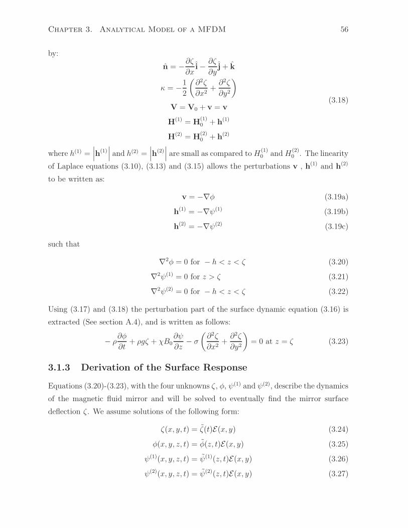
Chapter 3. Analytical Model of a MFDM 56
by:
n = −∂ζ∂x
i − ∂ζ
∂yj + k
κ = −1
2
(∂2ζ
∂x2+∂2ζ
∂y2
)
V = V0 + v = v
H(1) = H(1)0 + h(1)
H(2) = H(2)0 + h(2)
(3.18)
where h(1) =∣∣∣h
(1)∣∣∣ and h(2) =
∣∣∣h
(2)∣∣∣ are small as compared toH
(1)0 andH
(2)0 . The linearity
of Laplace equations (3.10), (3.13) and (3.15) allows the perturbations v , h(1) and h(2)
to be written as:
v = −∇φ (3.19a)
h(1) = −∇ψ(1) (3.19b)
h(2) = −∇ψ(2) (3.19c)
such that
∇2φ = 0 for − h < z < ζ (3.20)
∇2ψ(1) = 0 for z > ζ (3.21)
∇2ψ(2) = 0 for − h < z < ζ (3.22)
Using (3.17) and (3.18) the perturbation part of the surface dynamic equation (3.16) is
extracted (See section A.4), and is written as follows:
− ρ∂φ
∂t+ ρgζ + χB0
∂ψ
∂z− σ
(∂2ζ
∂x2+∂2ζ
∂y2
)
= 0 at z = ζ (3.23)
3.1.3 Derivation of the Surface Response
Equations (3.20)-(3.23), with the four unknowns ζ , φ, ψ(1) and ψ(2), describe the dynamics
of the magnetic fluid mirror and will be solved to eventually find the mirror surface
deflection ζ . We assume solutions of the following form:
ζ(x, y, t) = ζ(t)E(x, y) (3.24)
φ(x, y, z, t) = φ(z, t)E(x, y) (3.25)
ψ(1)(x, y, z, t) = ψ(1)(z, t)E(x, y) (3.26)
ψ(2)(x, y, z, t) = ψ(2)(z, t)E(x, y) (3.27)

Chapter 3. Analytical Model of a MFDM 57
where
E(x, y) = e−i(kxx+kyy)
kx and ky are the mode numbers, and it is understood that only the real part of the
solution will be retained. The Laplace equation (3.20) can be solved using the assumed
solution (3.25) and two boundary conditions on φ. The first boundary condition is derived
from the free surface kinematic condition (3.7), which can be written as:
− ∂φ
∂z=∂ζ
∂tat z = ζ (3.28)
Considering that the surface deflection ζ is small in magnitude, condition (3.28) is written
at z = 0 instead of z = ζ . The second condition is deduced from the physical consider-
ation that there cannot be any flow across the solid surface at the bottom of the fluid
layer, which implies
− ∂φ
∂z= 0 at z = −h (3.29)
The resulting solution is as follows (For a detailed solutions of the Laplace equations
(3.20)-(3.22) see section A.5):
φ(x, y, z, t) = −1
k
cosh (k(z + h))
sinh (kh)
dζ(t)
dtE(x, y) (3.30)
where
k =√
k2x + k2
y
and, depending on kx and ky, an infinite number of solutions can be obtained for φ.
Equations (3.21) and (3.22) are simultaneously solved using the following magnetic field
boundary conditions:
n×(
H(2) − H(1))
= 0 at z = ζ (3.31a)
n ·(
B(2) − B(1))
= 0 at z = ζ (3.31b)
limz→∞
ψ(1) <∞ (3.31c)
ψ(x, y, z, t) =
L∑
l=1
ψl(t)δ2(x− xl)(y − yl) at z = −h (3.31d)
The standard boundary condition (3.31a) states that, at the interface of the fluid and
the air, the tangential components of the magnetic fields in the two media are equal.
Similarly, condition (3.31b) signifies that the normal components of the magnetic flux

Chapter 3. Analytical Model of a MFDM 58
densities in the two media are also equal at the interface. Again, keeping in view the
small magnitude of ζ , these two conditions are written at z = 0 instead of z = ζ .
Condition (3.31c) implies that the magnetic field in the region above the free surface
remains bounded. Condition (3.31d) specifies the magnetic field resulting from the point
sources of magnetic potential applied at the bottom of the fluid layer. Using (3.31a)-
(3.31c) the following solutions are obtained for ψ(1) and ψ(2), respectively:
ψ(1)(x, y, z, t) = A(t)e−kzE(x, y) (3.32a)
ψ(2)(x, y, z, t) =
A(t)
(
cosh(kz) − µ
µsinh(kz)
)
− χ
µB0ζ(t) cosh(kz)
E(x, y) (3.32b)
where A(t) is the integration constant that will be later determined using (3.31d).
Application of the condition that the components of velocity normal to the container
walls must be zero yields the following mode shapes
E(x, y) = cos(kxx) cos(kyy) (3.33)
and the characteristic equations
sin kxx = 0 at x = Lx (3.34)
sin kyy = 0 at y = Ly (3.35)
The conditions (3.34) and (3.35) can be satisfied by an infinite number of discrete values
of kx and ky, which can be written in the series form as
kx = (m−1)πLx
for m = 1, 2, 3 · · ·ky = (n−1)π
Lyfor n = 1, 2, 3 · · ·
Now applying the input magnetic potential (3.31d) as a boundary condition on ψ(2) at
z = −h and making use of the orthogonality property of the mode shapes, the unknown
constant A(t) can be determined for each mode as:
Amn(t) =1
cosh(kmnh) + µµ
sinh(kmnh)(
χ
µB0 cosh(kmnh)ζmn(t) +
cmcnLxLy
L∑
l=1
ψl(t) cos(kmxl) cos(knyl)
)
(3.36)

Chapter 3. Analytical Model of a MFDM 59
where the subscripts m, n and mn have been affixed to show that the mode numbers kx,
ky and k, as well as the variables dependent on them, can take only discrete values, and
cm =
1 for m = 1
2 for m > 1
cn =
1 for n = 1
2 for n > 1
Now that the scalar potentials φ, ψ(1) and ψ(2) have been determined as given in
(3.30), (3.32a) and (3.32b), their substitution into the surface dynamic equation (3.23)
gives
ρ1
kmn
1
tanh(kmnh)
d2ζmn(t)
dt2+ ρgζmn(t) + σk2
mnζmn(t) −χµ
µB0kmnAmn(t) = 0 (3.37)
Further substitution of (3.36) into (3.37), followed by its rearrangement, yields
d2ζmn(t)
dt2+ ω2
mnζmn(t) = fmn(t) (3.38)
where
ω2mn = g tanh(kmnh)kmn +
σ
ρtanh(kmnh)k
3mn −
χ2
µ
B20
ρ
sinh(kmnh)µµ
cosh(kmnh) + sinh(kmnh)k2mn
(3.39)
fmn(t) = Fmn
L∑
l=1
ψl(t)E lmn (3.40)
Fmn = χB0
ρ
tanh(kmnh)µµ
cosh(kmnh) + sinh(kmnh)k2mn
cmcnLxLy
(3.41)
E lmn = cos(kmxl) cos(knyl) (3.42)
The second order differential equation (3.38) can be solved to obtain the generalized
displacements ζmn(t). The generalized displacements and the corresponding mode shapes
Emn , evaluated at any desired location (xk, yk), give the total surface displacement at
the location as:
ζk(xk, yk, t) =
∞∑
m=1
∞∑
n=1
ζmn(t)Emn(xk, yk) (3.43)
The damping effect associated with the fluid viscosity may be introduced into the model
by adding a factor of ωdmn
dζmn(t)dt
to the left-hand side of (3.38) [109], where
ωdmn= 4
η
ρk2mn
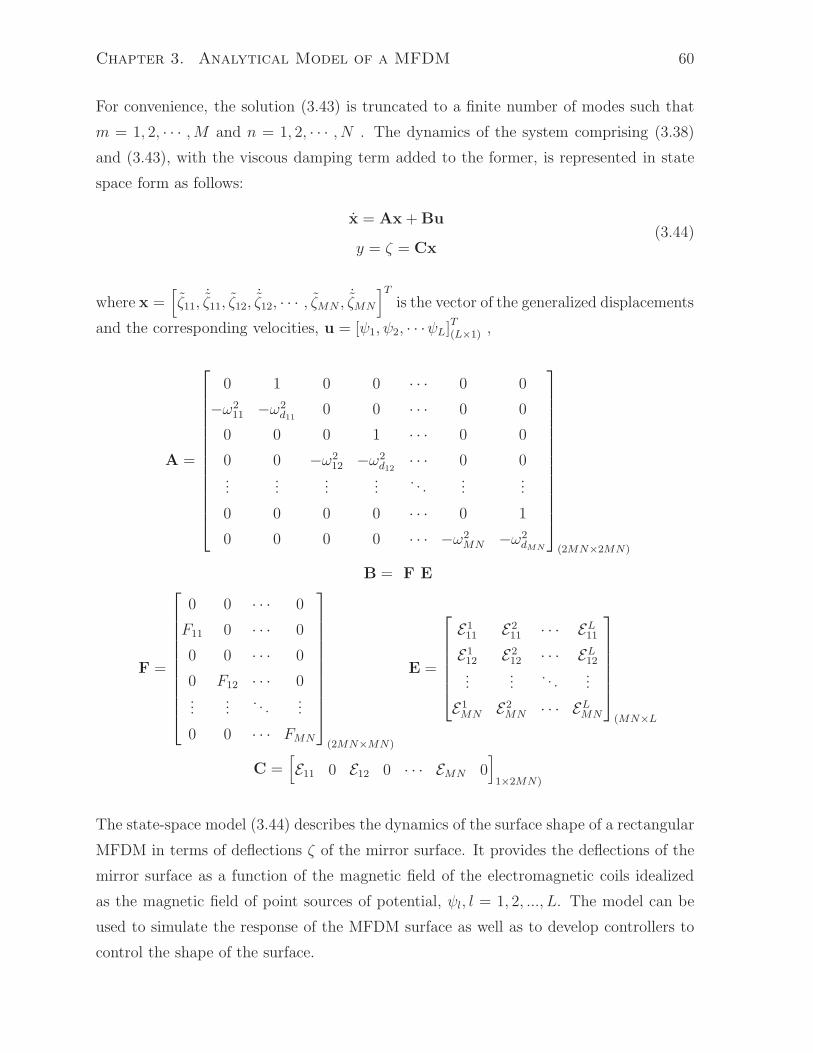
Chapter 3. Analytical Model of a MFDM 60
For convenience, the solution (3.43) is truncated to a finite number of modes such that
m = 1, 2, · · · ,M and n = 1, 2, · · · , N . The dynamics of the system comprising (3.38)
and (3.43), with the viscous damping term added to the former, is represented in state
space form as follows:
x = Ax + Bu
y = ζ = Cx(3.44)
where x =[
ζ11,˙ζ11, ζ12,
˙ζ12, · · · , ζMN ,˙ζMN
]T
is the vector of the generalized displacements
and the corresponding velocities, u = [ψ1, ψ2, · · ·ψL]T(L×1) ,
A =
0 1 0 0 · · · 0 0
−ω211 −ω2
d110 0 · · · 0 0
0 0 0 1 · · · 0 0
0 0 −ω212 −ω2
d12· · · 0 0
......
......
. . ....
...
0 0 0 0 · · · 0 1
0 0 0 0 · · · −ω2MN −ω2
dMN
(2MN×2MN)
B = F E
F =
0 0 · · · 0
F11 0 · · · 0
0 0 · · · 0
0 F12 · · · 0...
.... . .
...
0 0 · · · FMN
(2MN×MN)
E =
E111 E2
11 · · · EL11E1
12 E212 · · · EL12
......
. . ....
E1MN E2
MN · · · ELMN
(MN×L
C =[
E11 0 E12 0 · · · EMN 0]
1×2MN)
The state-space model (3.44) describes the dynamics of the surface shape of a rectangular
MFDM in terms of deflections ζ of the mirror surface. It provides the deflections of the
mirror surface as a function of the magnetic field of the electromagnetic coils idealized
as the magnetic field of point sources of potential, ψl, l = 1, 2, ..., L. The model can be
used to simulate the response of the MFDM surface as well as to develop controllers to
control the shape of the surface.

Chapter 3. Analytical Model of a MFDM 61
θ
Figure 3.2: Geometric representation of a circular magnetic fluid deformable mirror.
3.2 Analytical Model in Circular Geometry
Almost all optical systems are designed and described in circular geometry. It is, there-
fore, pertinent to extend the model presented in the previous section to circular geometry.
Accordingly, this section describes the model of a MFDM in a cylindrical coordinate sys-
tem.
As shown in Figure 3.2, the MFDM is represented by a cylindrical horizontal layer of
a magnetic fluid. The top free surface of the fluid layer serves as the deformable mirror.
The shape of the mirror is described by the deflection ζ(r, θ, t) of the deformable surface as
measured with respect to a point (r, θ) in the horizontal plane. The deflection is produced
by the cumulative magnetic field generated by an array of miniature electromagnetic coils
located underneath the magnetic fluid layer. The magnetic field generated by any given
coil l, l = 1, 2, · · · , L, centered at the horizontal location (rl, θl) , is idealized as that of a
point source of magnetic potential ψl(t).
3.2.1 Simplified Governing Equations
Since the system of governing equations (3.1)-(3.8) is presented in operator notation, it
is equally valid for the cylindrical coordinate system. Also, the simplifications given in
section 3.1.2 are independent of coordinate system and hence remain valid for the analysis
presented in this section. Using these simplifications, the set of equations (3.1)-(3.8) can
be reduced to [110]:
∇2Φ = 0 for − d < z < ζ (3.45)
∇2Ψ(i) = 0 i = 1, 2, 3 (3.46)
−ρ∂Φ∂t
+ ρgζ − µχ
2
(
∇Ψ(2) · ∇Ψ(2) + χ(∇Ψ(2) · n
)2)
+ p(1) + 2σκ = 0 at z = ζ (3.47)

Chapter 3. Analytical Model of a MFDM 62
where Φ(r, θ, z, t) is a scalar potential that describes the fluid velocity vector V as follows:
V = −∇Φ (3.48)
Note that in this case, the point sources of magnetic potential are placed underneath the
magnetic fluid layer and are not restricted to the fluid domain boundary. Considering
that the magnetic field extends into the space above and below the fluid layer, Maxwell’s
equations are applied to all three sub-domains marked in Figure 3.2 as (1), (2) and (3).
The scalar potentials Ψ(i), i = 1, 2, 3 describe the magnetic field vectors H(i) in these
sub-domains as follows:
H(i) = −∇Ψ(i) = 0 i = 1, 2, 3 (3.49)
The set of equations (3.45)-(3.47) can be solved to obtain the five unknowns ζ,Φ and
Ψ(i), i = 1, 2, 3 . Again, the surface dynamic equation (3.47) is nonlinear in Ψ(2), which
not only complicates the solution of the equations but also has implications in the eventual
control of the fluid surface. To circumvent the nonlinearity in (3.47), we introduce a large
uniform magnetic field with a constant flux density B0 superimposed on the input field
generated by the array of miniature coils.
The magnetic fluid mirror is considered to be in an initial equilibrium state char-
acterized by a perfectly flat horizontal surface (ζ = 0) and the uniform magnetic flux
B0 applied vertically across the whole fluid volume. The fluid is then perturbed by the
magnetic field resulting from the input potentials ψl, l = 1, 2, · · · , L. Assuming small
perturbations of all the field quantities and retaining only first order terms, the pertur-
bation part of (3.45)-(3.47) is extracted as given below:
∇2φ = 0 for − d < z < ζ (3.50)
∇2ψ(i) = 0 i = 1, 2, 3 (3.51)
−ρ∂φ∂t
+ ρgζ + χB0∂ψ(2)
∂z− σ
(∂2ζ
∂r2+
1
r
∂ζ
∂r+
1
r2
∂2ζ
∂θ2
)
= 0 at z = ζ (3.52)
where φ and ψ(i), i = 1, 2, 3 are the perturbation components of the scalar potentials
Φ and Ψ(i) i = 1, 2, 3 , respectively. Note that only the vertical component of the field
generated by the miniature coils i.e., hz = −∂ψ(2)
∂z, appears in the linearized surface
dynamic equation (3.52) and that the component is being multiplied by the uniform
vertical field B0. These features will be referred to in the design of the prototype MFDM
presented in chapter 4.

Chapter 3. Analytical Model of a MFDM 63
3.2.2 Derivation of the Surface Response
Equations (3.50)-(3.52), with the five unknowns ζ, φ and ψ(i), i = 1, 2, 3 describe the
dynamics of the magnetic fluid mirror and will be solved to eventually find the mirror
surface deflection ζ . We assume the following separable solutions:
ζ(r, θ, t) = ζ(t)R(r)Θ(θ) (3.53a)
φ(r, θ, z, t) = φ(z, t)R(r)Θ(θ) (3.53b)
ψ(i)(r, θ, z, t) = ψ(z, t)R(r)Θ(θ), i = 1, 2, 3 (3.53c)
The Laplace equation (3.50) is solved using the assumed solution (3.53b) and the following
two boundary conditions:
−∂φ∂z
=∂ζ
∂tat z = ζ (3.54)
−∂φ∂z
= 0 at z = −d (3.55)
The condition (3.54) is derived from the kinematic condition (3.7), and (3.55) has been
deduced from the physical consideration that there cannot be any flow across the solid
surface at the bottom of the layer. Considering the surface deflection ζ to be small in
magnitude, condition (3.54) is written at z = 0 instead of z = ζ . The solution thus
obtained is as follows:
φ(r, θ, z, t) = −1
λ
cosh (λ(z + d))
sinh (λd)
dζ(t)
dtR(r)Θ(θ) (3.56)
where λ is the separation constant, and where R(r) and Θ(θ) satisfy the following ordi-
nary differential equations [111]:
d2Θ
dθ2+m2Θ = 0 (3.57)
(d2Rdr2
+1
r
dRdr
)
+
(
λ2 − m2
r2
)
R = 0 (3.58)
where m is another separation constant.
The magnetic field equations (3.51) are simultaneously solved using the following bound-
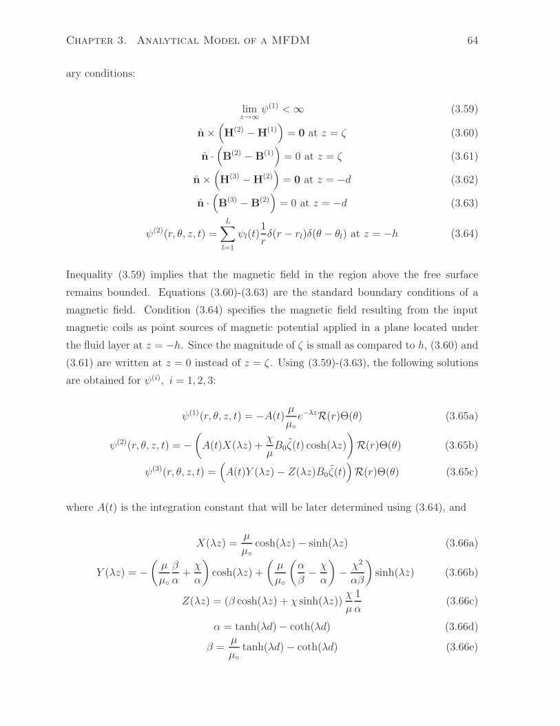
Chapter 3. Analytical Model of a MFDM 64
ary conditions:
limz→∞
ψ(1) <∞ (3.59)
n×(
H(2) − H(1))
= 0 at z = ζ (3.60)
n ·(
B(2) − B(1))
= 0 at z = ζ (3.61)
n×(
H(3) − H(2))
= 0 at z = −d (3.62)
n ·(
B(3) − B(2))
= 0 at z = −d (3.63)
ψ(2)(r, θ, z, t) =
L∑
l=1
ψl(t)1
rδ(r − rl)δ(θ − θl) at z = −h (3.64)
Inequality (3.59) implies that the magnetic field in the region above the free surface
remains bounded. Equations (3.60)-(3.63) are the standard boundary conditions of a
magnetic field. Condition (3.64) specifies the magnetic field resulting from the input
magnetic coils as point sources of magnetic potential applied in a plane located under
the fluid layer at z = −h. Since the magnitude of ζ is small as compared to h, (3.60) and
(3.61) are written at z = 0 instead of z = ζ . Using (3.59)-(3.63), the following solutions
are obtained for ψ(i), i = 1, 2, 3:
ψ(1)(r, θ, z, t) = −A(t)µ
µ
e−λzR(r)Θ(θ) (3.65a)
ψ(2)(r, θ, z, t) = −(
A(t)X(λz) +χ
µB0ζ(t) cosh(λz)
)
R(r)Θ(θ) (3.65b)
ψ(3)(r, θ, z, t) =(
A(t)Y (λz) − Z(λz)B0ζ(t))
R(r)Θ(θ) (3.65c)
where A(t) is the integration constant that will be later determined using (3.64), and
X(λz) =µ
µcosh(λz) − sinh(λz) (3.66a)
Y (λz) = −(µ
µ
β
α+χ
α
)
cosh(λz) +
(µ
µ
(α
β− χ
α
)
− χ2
αβ
)
sinh(λz) (3.66b)
Z(λz) = (β cosh(λz) + χ sinh(λz))χ
µ
1
α(3.66c)
α = tanh(λd) − coth(λd) (3.66d)
β =µ
µ
tanh(λd) − coth(λd) (3.66e)

Chapter 3. Analytical Model of a MFDM 65
Equation (3.57) has well known periodic solutions cosmθ and sinmθ, and results in the
following eigen functions:
Θ(θ) =
sinmθ m = 1, 2, 3, · · ·
cosmθ m = 0, 1, 2, · · ·(3.67)
Equation (3.58) is Bessel’s equation, which can be solved for each m and has the general
solution of the following form:
R(t) = C1Jm(λr) + C2Ym(λr) (3.68)
where C1 and C2 are constants of integration and Jm(λr) and Ym(λr) are the Bessel
functions of the first and the second kind, respectively, each of order m. The condition
that both magnetic and fluid potentials are bounded throughout the domain can be
satisfied only if C2 = 0, which results in:
R(t) = C1Jm(λr) (3.69)
Further considering that the miniaturized coils are located far from the walls of the fluid
container, (3.69) yields the following characteristic equation
Jm(λr) = 0 at r = R (3.70)
Equation (3.70) can be solved numerically and yields an infinite number of solutions
ǫmn = λR , m = 0, 1, 2, · · · , n = 1, 2, 3, · · · , providing the eigenvalue λmn for each mode
as follows:
λmn =ǫmnR
(3.71)
Equations (3.67) and (3.69) can be combined to obtain the following permissible mode
shapes:
Hmnc = Jm(λmnr) cos(mθ)
Hmns = Jm(λmnr) sin(mθ)(3.72)
Applying the input magnetic potential (3.64) as a boundary condition on ψ(3) at z = −hand making use of the orthogonality property of the mode shapes (3.72), the unknown
constant A(t) can be determined for each mode as:
Amnc(t) =1
Y (−λmnh)
(
Z(−λmnh)B0ζmnc(t) +k
πR2 [Jm+1(ǫmn)]2
L∑
l=1
ψl(t)Jm(λmnrl) cos(mθl)
)
(3.73)

Chapter 3. Analytical Model of a MFDM 66
for m = 0, 1, 2, · · ·n = 1, 2, 3, · · · , and
Amns(t) =1
Y (−λmnh)
(
Z(−λmnh)B0ζmns(t) +k
πR2 [Jm+1(ǫmn)]2
L∑
l=1
ψl(t)Jmn(λmnrl) sin(mθl)
)
(3.74)
for m,n = 1, 2, 3, · · · where
k =
1 for m = 0
2 for m 6= 0(3.75)
With the integration constant A(t) obtained as Amnc(t) (3.73) and Amns(t) (3.74), the
scalar potentials φ and ψ(i), i = 1, 2, 3 are fully determined as given in (3.56) and (3.65a)-
(3.65c), and, for the case of symmetric modes (cosmθ), their substitution into the surface
dynamic equation (3.52) gives
ρ1
λmn
1
tanh(λmnd)
d2ζmnc(t)
dt2+ ρgζmnc(t) + σλ2
mnζmnc(t) + χB0λmnAmnc(t) = 0 (3.76)
Further substitution of (3.73) into (3.76), followed by its rearrangement, yields
d2ζmnc(t)
dt2+ ω2
mnζmnc(t) = fmnc(t) (3.77)
where
ω2mn = g tanh(λmnd)λmn +
σ
ρtanh(λmnd)λ
3mn +
χ
ρB2
0 tanh(λmnh)λ2mn
Z(−λmnh)Y (−λmnh)
(3.78)
fmnc(t) = Fmn
L∑
l=1
ψl(t)Hlmnc (3.79)
Fmn = −χB0
ρ
tanh(λmnh)
Y (−λmnh)λ2mn
k
πR [Jm+1(ǫmn)]2 (3.80)
Hlmnc = Jm(λmnrl) cos(mθl) (3.81)
for m = 0, 1, 2, · · ·n = 1, 2, 3, · · · , l = 1, 2, 3, · · · , L.
Using (3.74), a similar set of equations can be obtained for the anti-symmetric modes
(sinmθ) as follows:
d2ζmns(t)
dt2+ ω2
mnζmns(t) = fmns(t) (3.82)
fmns(t) = Fmn
L∑
l=1
ψl(t)Hlmns (3.83)
Hlmns = Jm(λmnrl) sin(mθl) (3.84)

Chapter 3. Analytical Model of a MFDM 67
for m,n = 1, 2, 3, · · · , l = 1, 2, 3, · · · , L.
The generalized displacements ζmnc(t) and ζmns(t), obtained from the solution of the
second order differential equations (3.77) and (3.82), respectively, and the corresponding
mode shapes Hmnc and Hmns evaluated at any desired location (rk, θk), give the total
surface displacement as:
ζk(rk, θk, t) =∞∑
m=0
∞∑
n=1
ζmnc(t)Hmnc(rk, θk) +∞∑
m=1
∞∑
n=1
ζmns(t)Hmns(rk, θk) (3.85)
The damping effects associated with the fluid viscosity may be introduced into the model
by adding the factors ωdmn
dζmnc(t)dt
and ωdmn
dζmns(t)dt
to the left-hand side of (3.77) and
(3.82), respectively. The damping frequency ωdmncan be approximated as follows [109]:
ωdmn= 4
η
ρλ2mn
The solution (3.85) is truncated to a finite number of modes such that m = 0, 1, 2, · · · ,Mand n = 1, 2, 3, · · · , N . Similarly, the surface deflection ζk(rk, θk, t) as provided by (3.85),
is limited to a discrete number of surface locations k, k = 1, 2, ..., K. The dynamics of
the system comprising (3.77), (3.82) and (3.85), with the viscous damping terms added
to the first two, is represented in the state space form as follows:
x = Ax + B′
u′
y = Cx(3.86)
where x =[
ζ01,˙ζ01, ζ02,
˙ζ02, · · · ζ0N , ˙
ζ0N , ζ11c,˙ζ11c, ζ11s,
˙ζ11s, ζ12c,
˙ζ12c, ζ12s,
˙ζ12s,· · · ,
ζMNc,˙ζMNc, ζMNs,
˙ζMNs
]T
is the vector of the generalized displacements and the corre-
sponding velocities collectively defining the states of the system, u′
= [ψ1, ψ2, · · ·ψL]T(L×1)
is the vector of input magnetic potentials and y = [ζ1, ζ2, ..., ζK]T(K×1) is the vector of
surface deflections defining the system output. With the system order determined as
Nd = 2N(2M + 1), the system matrices A ∈ RNd×Nd , B
′ ∈ RNd×L and C ∈ R
K×Nd are
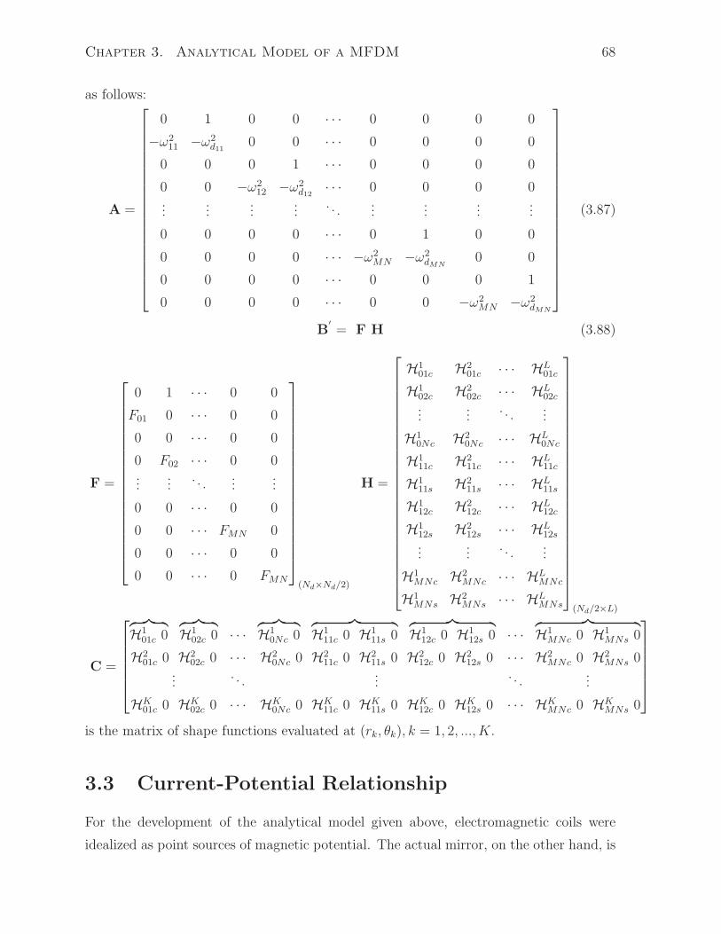
Chapter 3. Analytical Model of a MFDM 68
as follows:
A =
0 1 0 0 · · · 0 0 0 0
−ω211 −ω2
d110 0 · · · 0 0 0 0
0 0 0 1 · · · 0 0 0 0
0 0 −ω212 −ω2
d12· · · 0 0 0 0
......
......
. . ....
......
...
0 0 0 0 · · · 0 1 0 0
0 0 0 0 · · · −ω2MN −ω2
dMN0 0
0 0 0 0 · · · 0 0 0 1
0 0 0 0 · · · 0 0 −ω2MN −ω2
dMN
(3.87)
B′
= F H (3.88)
F =
0 1 · · · 0 0
F01 0 · · · 0 0
0 0 · · · 0 0
0 F02 · · · 0 0...
.... . .
......
0 0 · · · 0 0
0 0 · · · FMN 0
0 0 · · · 0 0
0 0 · · · 0 FMN
(Nd×Nd/2)
H =
H101c H2
01c · · · HL01c
H102c H2
02c · · · HL02c
......
. . ....
H10Nc H2
0Nc · · · HL0Nc
H111c H2
11c · · · HL11c
H111s H2
11s · · · HL11s
H112c H2
12c · · · HL12c
H112s H2
12s · · · HL12s
......
. . ....
H1MNc H2
MNc · · · HLMNc
H1MNs H2
MNs · · · HLMNs
(Nd/2×L)
C =
︷ ︸︸ ︷
H101c 0
︷ ︸︸ ︷
H102c 0 · · ·
︷ ︸︸ ︷
H10Nc 0
︷ ︸︸ ︷
H111c 0 H1
11s 0︷ ︸︸ ︷
H112c 0 H1
12s 0 · · ·︷ ︸︸ ︷
H1MNc 0 H1
MNs 0
H201c 0 H2
02c 0 · · · H20Nc 0 H2
11c 0 H211s 0 H2
12c 0 H212s 0 · · · H2
MNc 0 H2MNs 0
.... . .
.... . .
...
HK01c 0 HK
02c 0 · · · HK0Nc 0 HK
11c 0 HK11s 0 HK
12c 0 HK12s 0 · · · HK
MNc 0 HKMNs 0
is the matrix of shape functions evaluated at (rk, θk), k = 1, 2, ..., K.
3.3 Current-Potential Relationship
For the development of the analytical model given above, electromagnetic coils were
idealized as point sources of magnetic potential. The actual mirror, on the other hand, is

Chapter 3. Analytical Model of a MFDM 69
controlled using currents applied to the coils. To generate corresponding surface responses
using the analytical model, it is necessary to establish a relationship between the current
input to a coil and the value of the magnetic potential of the corresponding point source.
The current-potential relationship is determined as follows.
Firstly, the position of the point source w.r.t the corresponding coil is fixed. Since
the contribution of the top turns of the coil to the magnetic field observed at the surface
of the fluid is much more significant than that of the lower turns, it is assumed that the
point source of potential is located at the same position as that of the center of the top
turns of the coil.
Secondly, using arbitrary values of current in the coil, the magnetic field of the actual
coil is simulated using COMSOL MultiphysicsTM (finite element analysis software by
COMSOL Inc. Stockholm, Sweden) and the values of the magnetic flux density at the
location corresponding to a point on the liquid surface immediately above the center
of the coil are determined. Then, using the derived analytical model, the values of
the point source of potential that yield the same values for the magnetic flux density
at the corresponding location are computed. The slope of the linear current-potential
relationship is then determined based on the obtained data. Actually, only two points
are sufficient since the relationship is found to be linear.
The current-potential relationship for the prototype MFDM described in the next
chapter is given in Figure 3.3. The relationship is based on the COMSOL simulation
of the actual coils used in the prototype MFDM (see Table 4.1 for the coil specification
used in the simulation). The relationship is determined for one electromagnetic coil and
is then applied uniformly across all others in the array. It should be noted that this
relationship was determined independently of the experimental data.
If α is the slope of the current-potential relationship, then
u′
= αu (3.89)
where u is the vector of currents ul, l = 1, 2, 3, ..., L, applied to the electromagnetic coils.
Using (3.89), the model (3.86) can be re-written as follows:
x = Ax + Bu
y = Cx(3.90)

Chapter 3. Analytical Model of a MFDM 70
0 10 20 30 400
1
2
3
4
5
6
7
8
9
10
Mag
netic
pot
entia
l, ψ (
× 10
−7 )
Current (× 10−3A)
1 2.36
25×
10−
6
0 10 20 30 400
0.05
0.1
0.15
0.2
0.25
0.3
0.35
Mag
netic
flux
den
sity
, b z (
× 10
−3 T
)
Figure 3.3: Current potential relationship.
where B = αB′
. A discrete-time equivalent representation of model (3.90) is given by:
x(k + 1) = Adx(k) + Bdu(k)
y(k) = Cx(k)(3.91)
where x(k) is the vector of state variables, u(k) is the vector of control currents, y(k) is
the vector of the mirror surface deflections and, Ad and Bd are the system matrices.
The DC gain of the system relating the steady state response yss to a vector of static
inputs uss can be obtained as
G0 = −CA−1B (3.92)
in the case of continuous time system and as
G0 = C(I − Ad)−1Bd (3.93)
in the case of discrete-time system.
3.4 Simulation of the MFDM Model
The analytical model presented above can be used to simulate the response of the MFDM
surface to the magnetic field generated by an array of electromagnetic coils. The model

Chapter 3. Analytical Model of a MFDM 71
Density 1210 Kg/m3
Viscosity 5.8 cP
Saturation Magnetization 40 mT
Relative Permeability 1.78
Coefficient of Surface Tension 29 × 10−3 N/m
Table 3.1: Properties of EFH1, the magnetic fluid used in the prototype MFDM.
provides the static as well as the dynamic surface shapes produced by the applied mag-
netic field. In the following, the analytical model representing the prototype MFDM
presented in the next chapter is simulated. The same simulations will be utilized later
in chapter 6 to validate the analytical model by comparing the results predicted by the
model to the experimental results obtained using the prototype mirror.
3.4.1 Model Parameters
The MFDM is modeled as a layer of EFH1 (Ferrofluid for Education - Hydrocarbon
type), which is a commercially available oil-based magnetic fluid (Ferrotec Corporation,
NH, USA). The properties of the fluid used in the simulation are given in Table 3.1. The
fluid layer has the following dimensions:
d = 1.0 mm, R = 30 mm
The magnetic field is generated using an array of 19 electromagnetic coils arranged in a
circular pattern and placed at distance h = 2.0 mm below the undisturbed surface of the
mirror. To ensure accuracy, the actual location of the coils measured in the prototype
mirror is used in the model. The location (rl(mm), θl(rad)), l = 1, 2, ..., 19 of the coils
is given as:
(0, 0), (4.1, 4.7), (3.4, 5.6), (3.9, 0.8), (4.2, 1.7), (5.2, 2.7), (4.4, 3.8), (7.6, 4.8), ...
(7.4, 5.3), (7.0, 5.8), (7.5, 0), (7.4, 0.6), (7.1, 1.3), (8.3, 1.7), (7.8, 2.2), (9.2, 2.7), ...
(8.9, 3.1), (8.0, 3.7), (7.0, 4.2)
The slope of the current-potential relationship, α, as determined from the COMSOL
simulation of the actual electromagnetic coil, is set to 2.3625×10⁻⁶/A. A vertical, uniform
magnetic field with the flux density B0 = 2.5 mT is superimposed on the magnetic field

Chapter 3. Analytical Model of a MFDM 72
−10 −5 0 5 10
−10
−5
0
5
10
Radial Distance r (mm)
Sur
face
Def
lect
ion
ζ (µ
m)
31.7 mA
25.4 mA
19.0 mA
12.7 mA
6.3 mA
−6.3 mA
−12.7 mA
−19.0 mA
−25.4 mA
38.0 mA
−31.7 mA
−38.1 mA
Figure 3.4: The static surface shapes predicted by the analytical model.
generated by the array of coils. The factors considered in the selection of the field strength
are discussed in section 4.1.3.
The analytical model (3.90) obtained using these parameters is given in Appendix B.
The model was obtained by truncating the radial and azimuthal modes to N = 4, M =
4, respectively.
3.4.2 Static Response
The static response of the mirror surface shape can be obtained by setting x = 0 with
input u given as a vector of constant currents. Firstly, the response of the mirror surface
to the current applied to only one coil is simulated. The simulated static shapes of the
mirror surface obtained by applying constant currents to the coil located at (r1, θ1) are
plotted in Figure 3.4. Taking advantage of the symmetry of the surface shape generated
by the chosen coil i.e., the one in center of the mirror, only 2D shapes are shown in the
figure. As can be observed from the figure, application of current to a single coil results
in a Gaussian surface shape with its peak located immediately above the location of the
energized coil.
A 3D surface shape resulting from a specified set of input currents u = [0.1, 0.5, 0.4, ...
0.3, 0.1, −0.1, 0.2, 0.9, 0.7, 0.6, −0.5, 0.6, 0.1, −0.4, −0.9, −0.3, 0.5, −0.3, 0.4]T× 131.5
A
applied to the complete array of 19 coils is presented in Figure 3.5.

Chapter 3. Analytical Model of a MFDM 73
−10
−5
0
5
10
−10
−5
0
5
10
−10
−5
0
5
10
x (mm)y (mm)
ζ (µ
m)
Figure 3.5: 3D static surface shapes predicted by the analytical model.
3.4.3 Dynamic Response
The analytical model can be used to observe the dynamics of the mirror surface shape.
As an illustration of the ability of the model to capture the dynamic response of the
mirror surface, the surface deflections resulting from a step input applied to the center
coil are plotted in Figure 3.6. The figure shows the time history of the surface deflections
observed at a surface location immediately above the coil.
A comprehensive picture of the dynamics of the MFDM surface can be seen by drawing
the Bode plots of the MIMO model. Figure 3.7 shows the Bode plots for three selected
channels where the input is applied at the coils located at (r1, θ1), (r2, θ2) and (r10, θ10)
and the output surface deflections are observed at the surface points located immediately
above the respective coils. While a detailed discussion on the dynamics of the mirror
will follow in chapter 6, a few observations may be noted here. Note that plots on
the leading diagonal show the input-output relationship between an electromagnetic coil
input and the surface displacement obtained immediately above the same coil. The off-
diagonal plots, on the other hand, show the coupling effect between different input-output
channels. It is obvious that for any input coil the magnitude of the surface deflection

Chapter 3. Analytical Model of a MFDM 74
0 1 2 3 40
2
4
6
8
10
Sur
face
Def
lect
ion
(µm
)
Time (s)
0
5
10
15
20
25
30
35
Cur
rent
(m
A)
Figure 3.6: Response to a step input. The input current is applied to the center coil only
and the surface deflections are obtained at a point immediately above the same coil.
immediately above the coil is significantly higher than the magnitude of the deflections
obtained away from the coil. Also note that the coupling effect varies from channel to
channel. While an input to the coil located at (r1, θ1) results in an output at (r2, θ2) with
a significant magnitude, the magnitude of the resulting surface deflections at (r10, θ10) is
negligibly small.
3.5 Summary
An analytical model of the dynamics of the surface shape of a MFDM has been presented
in this chapter. The model is derived using a coupled system of equations obtained
from the fundamental governing principles of conservation of mass and momentum, and
Maxwell’s equations. The model describes the dynamics of the mirror surface shape in
terms of deflections of the mirror surface produced by a magnetic field generated by an
array of electromagnetic coils. The model has been developed in both the Cartesian and
the cylindrical coordinate systems. An innovative method of linearizing the equations
governing the dynamics of the mirror surface was introduced and will be utilized to
propose an important modification in the design of a MFDM. The developed model was
presented in state-space form and was used to simulate the static as well as the dynamic
response of the mirror surface shape.

Chapter 3. Analytical Model of a MFDM 75
0
5
10From: In(1)
To:
Out
(1)
−270−180−90
0
To:
Out
(1)
0
5
10
To:
Out
(2)
−270−180−90
0
To:
Out
(2)
0
5
10
To:
Out
(3)
10−1
100
101
102
−270−180−90
0
To:
Out
(3)
From: In(2)
10−1
100
101
102
From: In(3)
10−1
100
101
102
Frequency (rad/sec)
Mag
nitu
de (
abs)
; P
hase
(de
g)
Figure 3.7: Bode plot of the MFDM model. The array of bode plots shows the system
response for three selected input-output channels. The inputs In(1), In(2) and In(3)
correspond to the electromagnetic coils l = 1, 2, and 10, respectively. The three plots
in the top row are the magnitude plots of the output surface deflections predicted by
the model for the location immediately above the center of coil #1. The second row
shows the corresponding phase plots. The magnitude and phase plots for the predicted
deflections above coils #2 and #10 are given alternatively in the following rows of plots.

Chapter 4
Design of a Magnetic Fluid
Deformable Mirror and the
Experimental Setup
This chapter presents the development of an adaptive optics experimental setup to be
used in the validation of the analytical model presented in chapter 3 and in testing the
controllers presented in chapter 5. The setup comprises a prototype MFDM and a closed-
loop AO system built around this wavefront corrector. The system can be complemented
by an imaging system to realize a functional ophthalmic imaging AO system. This chapter
provides a description of the important considerations in the design of the mirror and the
encompassing AO system. The conceptual and detailed designs the prototype MFDM
are presented in the next section. The design of the experimental AO system and a
description of its main components are presented in section 4.2.
4.1 Design of Magnetic Fluid Deformable Mirror
The design of a practically deployable MFDM involves a wide range of considerations
including - just to name a few - the application-specific performance requirements, main-
tainability and cost constraints. Covering all these aspects is beyond the scope of this
work. However, in what follows, we will examine important design features of a MFDM
that affect the control of the mirror and its application in ophthalmic imaging systems.
76

Chapter 4. Design of a MFDM and the Experimental AO Setup 77
4.1.1 Conceptual Design
Conventional Conceptual Design
The basic operating principle of a MFDM was briefly described in section 2.3 and the
schematic layout of the conventional design of the mirror was shown in Figure 2.20. The
primary elements of the mirror are a layer of a magnetic fluid, a thin film of a reflective
material coated on the free surface of the fluid and an array of electromagnetic coils
placed beneath the fluid layer. Each of the electromagnetic coils is driven independently
by applying a corresponding current input. The combined electromagnetic field of the
coils causes the fluid surface and the reflective film to deform. The deformed reflective
surface acts as a mirror whose shape can be controlled by adjusting the current applied to
the individual coils. The material properties of the magnetic fluid and the reflective film,
the shape and size of the fluid layer, the number and arrangement of the electromagnetic
coils, and the dimensions of each coil are the variables that need to be established in the
detailed design process.
Modified Design
The analytical work undertaken to develop a model of a MFDM, as given in chapter
3, revealed that the deflection of the magnetic fluid surface is non-linear in the applied
magnetic field. This non-linearity results in a fundamental limitation of the conventional
MFDM design: since the surface displacement is a quadratic function of the applied
magnetic field, only positive displacements can be achieved. It has already been known
that the magnetic field of electromagnetic coils in conventional configuration can displace
the magnetic fluid in the upward direction only i.e., the magnetic field can ’push’ the
fluid surface but cannot ’pull’ [15]. As it was briefly introduced in section 3.1.2, one of
the solutions to the problem of non-linear response of the fluid surface is to linearize it
by superimposing a large, uniform, vertical magnetic field on the field generated by the
electromagnetic coils. The proposed modified design is the realization of this solution,
where a large uniform magnetic field generated by an appropriate source is superimposed
on the magnetic field of the conventionally used array of coils.
A Helmholtz coil is one of the many means available to generate the uniform magnetic
field. As shown in Figure 4.1, it consists of two circular coils of equal diameter, which are
separated by a distance equal to the radius of the coils. This distinctive design provides
a magnetic field, which runs parallel to the central axis and is uniform over a significant

Chapter 4. Design of a MFDM and the Experimental AO Setup 78
äåFigure 4.1: Layout of a Helmholtz coil.
volume extending around the axis.
The proposed modified design of a MFDM is a combination of a Helmholtz coil
and the conventional design as was illustrated in Figure 2.20. The modified design,
as shown in Figure 4.2, places the conventional MFDM inside the Helmholtz coil thus
allowing the uniform field of the Helmholtz coil to be superimposed on the field of the
coils placed underneath the fluid layer. The figure shows a more practical Helmholtz
coil with each of the two coils comprising multiple turns. For clarity, the coils placed
underneath the fluid layer will be referred to as miniature coils. If the magnetic field of
the Helmholtz coil is significantly larger than the field of the miniature coils, the surface
displacements become linearized in terms of the vertical component of the magnetic field
of the miniature coils. As alluded to in the theoretical work presented in section 3.1.2,
the horizontal components of the magnetic field can be ignored when the magnetic field
of the Helmholtz coil is present. The following are the main features of the proposed
design:
• The conventional mirror is placed inside the Helmholtz coil such that the central
axis of the coil is aligned with the gravity vector i.e., the uniform field of the coil
runs perpendicular to the free surface of the magnetic fluid.
• The strength of the uniform field is chosen to be significantly larger than the max-
imum magnetic field of each of the miniature coils.
• Contrary to the conventional configuration where the electromagnetic coils are aug-
mented with a soft magnetic core for increasing the flux density, the miniature coils
in the modified design are air-cored type. Theoretically, the coils with a soft mag-
netic core can still be used to serve the basic purpose of linearization of the response

Chapter 4. Design of a MFDM and the Experimental AO Setup 79
Figure 4.2: Modified conceptual design of a magnetic fluid deformable mirror.
of the fluid surface. However, they cause the magnetic field of the Helmholtz coil
to concentrate along the axes of the miniature coils submerged in the field of the
Helmholtz coil thus resulting in non-uniformities of the field. The resulting field
gradients cause deflections of the fluid surface even when no currents are applied
to the miniature coils.
• The diameter of the fluid layer is chosen to be significantly larger than the active
area containing the coils, which implies that the diameter of the fluid layer is
significantly larger that the optical pupil as measured on the fluid surface. This
feature ensures that the effects of the magnetic field gradients at the edges of the
fluid layer are excluded from the active mirror area. The gradients are caused by
the unavoidable discontinuity of magnetic permeability at the interface of the fluid
and the container. The exclusion of the edges is also desirable for the conventional
design as it avoids the meniscus along the walls of the container.

Chapter 4. Design of a MFDM and the Experimental AO Setup 80
4.1.2 Detailed Design
While the conceptual design provides only an outline of any product, the detailed design
is an iterative process that determines the definite values of the various design features
i.e., design variables, which meet a prescribed set of constraints and performance re-
quirements. Depending on the nature of the application, different sets of constraints and
performance requirements can be specified for the design of a MFDM. These requirements
in turn dictate what features should be considered as design variables. We consider a
generalized set of requirements and design variables as described below:
Design Requirements
Spatial Resolution. Spatial resolution or the number of spatial modes to be corrected
signify the degree of accuracy of correction required. The finer the extent of defects that
need to be compensated for, the higher the required order or the number of modes will
be.
Bandwidth. The bandwidth is the required operating frequency range of the deforma-
tion of the mirror surface. The requirement is dictated by the frequency of the aberrations
that need to be corrected.
Dynamic Range. The dynamic range defines the maximum and the minimum achiev-
able correction i.e., the magnitude of surface deflection that can be generated using the
MFDM. For example, a deformable mirror may be required to produce up to 10 microm-
eter deflection with a resolution of 10 nanometer. The stroke i.e., the maximum required
deflection of the mirror surface, is dictated by the depth of the aberrations that need to
be corrected. The requirement of the smallest applicable deflection is dictated by the
precision of the correction.
Design Variables
Number of Actuators and Actuator Spacing. The total number of actuators (elec-
tromagnetic coils) and spacing between them determines the spatial resolution or the
number of modes that can be corrected. For a given shape of the array of actuators, it
also determines the size of the active part of deformable mirror, which in turn determines

Chapter 4. Design of a MFDM and the Experimental AO Setup 81
the size of the AO system. A good approximation of the appropriate spacing can be ob-
tained from the empirical observation that most of the wavefront correctors currently in
use have 10%-20% coupling between two adjacent actuators [4]. The actuator spacing
that provides the desired coupling can be directly observed by ploting the surface shape
obtained by applying input to a single actuator.
Dimensions of the Miniature Coils. The strength of the magnetic field generated
by each magnetic coil as measured at the surface of the magnetic fluid is the principle
factor that controls the shape and magnitude of the resulting surface deflections. The
strength of the magnetic field generated by the coil is a function of the number of turns
in each coil, the length and diameter of the coil, and the maximum allowable current in
the coil.
In the modified design featuring a vertical, uniform magnetic field superimposed on
the field of the miniature coils, only the vertical component of the magnetic field of
the miniature coils plays the significant role. It serves to provide the desired shape
of deformation of the fluid surface while the large uniform field provides the necessary
amplification of the surface deflections.
Size of the Fluid Layer. The size of the fluid layer refers to the depth and diameter of
the layer. The depth of the fluid layer affects the stroke of the mirror i.e., the maximum
achievable surface deflections. As discussed in section 3.2, the magnitude of the mirror
surface deflection is a linear function of the vertical component, bz, of the magnetic field
of the miniature coils as observed at the mirror surface. The magnetic field component bz
itself can be varied by varying the vertical distance h between the top edge of the array
of electromagnetic coils and the deformable surface of the mirror. Therefore, keeping all
other factors constant, the maximum mirror surface deflection can be varied by varying
the depth of the fluid layer. As shown in Figure 4.3, the vertical component, bz, of
the magnetic field generated by an electromagnetic coil varies exponentially with the
variation of distance h. Consequently, any variation in the depth of the fluid layer also
causes an exponential change in the stroke of the mirror.
Magnetic Fluid Properties. Due to the synthetic nature of the magnetic fluids, the
properties of a fluid intended for an application can always be tailored according to the
requirements of the application. Therefore, the choice of appropriate fluid alone offers a

Chapter 4. Design of a MFDM and the Experimental AO Setup 82
0 1 2 3 4 50
0.5
1
1.5
h (mm)
b z (m
T)
Figure 4.3: The decay of the vertical component of the magnetic flux density (bz) of a
coil with an increasing distance, h, from the top edge of the coil.
great degree of freedom in the design of a MFDM. For example, the surface deflections
obtained using a given magnetic field can be greatly varied by using magnetic fluids with
different permeability or density. Similarly, the viscosity of the fluid affects the damping
properties of the fluid motion and hence is an important determinant of the dynamic
stability and controllability of the MFDM. Surface tension is another fluid property that
affects the surface response and will be discussed at greater length in chapter 6.
Design of the Helmholtz Coil
The nominal diameter (d in Figure 4.2) of the two circular coils, the number of turns in
each coil, and the maximum allowable current are the primary design variables pertaining
to a Helmholtz coil. The Helmholtz coil should be able to provide a magnetic field, which
is significantly (at least ten times) larger than the magnetic field of the miniature coils.
Also, the uniformity of the magnetic field generated by the Helmholtz coil deteriorates
with the increasing distance from the central axis. Therefore, the internal diameter
should be large enough to ensure a minimum specified uniformity.
4.1.3 Description of the Prototype MFDM
A MFDM comprising 19 input-channels has been developed for the experimental valida-
tion of the MFDM model and the controllers presented in this thesis. Though a clinically

Chapter 4. Design of a MFDM and the Experimental AO Setup 83
æçèèçéèè
Figure 4.4: Schematic diagram of the prototype MFDM.
deployable mirror should meet all of the requirements listed above, the mirror was built
as a proof-of-concept prototype, which meets only as many requirements as could be
accommodated within the limited time and resources available for the research work.
Figure 4.4 shows the schematic layout of the mirror. The pictorial view of the assembly
of the mirror is shown in Figure 4.5. The salient features of the mirror are as follows:
• The fluid element of the mirror comprises a 60mm diameter layer of EFH1 (Fer-
rofluid for Education - Hydrocarbon type) which is a commercially available oil-
based magnetic fluid (Ferrotec Corporation, NH, USA). The thickness of the layer
can be varied by adding appropriate volume of the fluid. Experiments were per-
formed using 1.0 mm thick layer. Important properties of the fluid are listed in
Table 3.1.
• The mirror is driven using an array of 19 electromagnetic coils arranged in a circular
pattern as shown Figure 4.6. The coils are radially spaced at 4 mm from center
to center thus presenting a total active footprint area of approximately 22 mm
diameter.
• The electromagnetic coils are conventional circular coils wound on a cylindrical
bobbin. The coils were obtained off-the-shelf from Dia-netics Inc., CA, USA, and
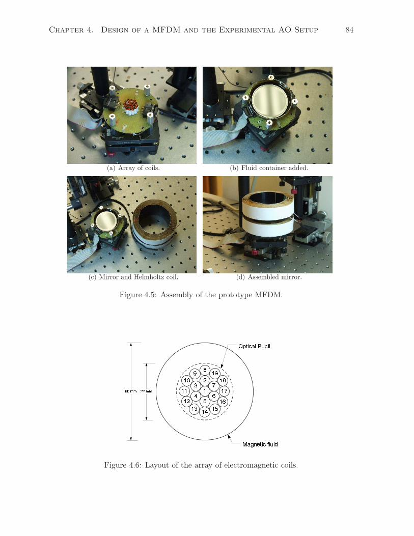
Chapter 4. Design of a MFDM and the Experimental AO Setup 84
(a) Array of coils. (b) Fluid container added.
(c) Mirror and Helmholtz coil. (d) Assembled mirror.
Figure 4.5: Assembly of the prototype MFDM.
êëì íîïð ñ êîêñêòêêêï êð êëêì êíó êóôõö÷øùúû üýþúÿ
ùúûõý þúý
Figure 4.6: Layout of the array of electromagnetic coils.

Chapter 4. Design of a MFDM and the Experimental AO Setup 85
Manufacturer’s part no. PCRC 408-006
Length 0.4 in (10.1 mm)
Internal diameter 0.084 in (2.1 mm)
External diameter incl. bobbin flange 0.137 in (3.5 mm)
No. of turns 620
No. of layers 4
Core-type Air-cored
Average resistance 31.5Ω
Wire gauge AWG41
Wire material Copper
Wire diameter (bare) 0.0028 in (0.071 mm)
Wire thickness incl. insulation 0.0029 in (0.074 mm)
Bobbin internal diameter 0.074 in (1.9 mm)
Bobbin wall thickness 0.005 in (0.125 mm)
Bobbin material Kapton R©
Table 4.1: Properties of the miniature electromagnetic coils.
have the properties/dimensions as given in Table 4.1.
• The Helmholtz coil was locally fabricated and has the properties/dimensions as
given in table 4.2. The strength of the magnetic field of the Helmholtz coil can be
controlled by varying the current applied to the coil. The coil is normally operated
at 194 mA, which produces a nominal magnetic flux density of 2.5 mT at the center
of the coil. The strength of the magnetic field is chosen such that it is sufficiently
larger than that of the miniature coils (bz ≈ 0.25) mT, as measured at the fluid
surface, but is safely below the critical limit (∼ 17 mT) at which the Rosensweig
instability occurs [93].
• The array of electromagnetic coils is driven by a PC-based system comprising a
PCI type analog voltage output card (National Instruments 6723) and a current
amplification and protection unit. The analog voltage card features 32 output volt-
age channels with a maximum update speed of 45 kS/s. With the 13 bit resolution,
it can provide voltages up to ±10 V at a precision of 2.4 mV. Since the analog
output voltage channels can supply only up to 5 mA current as against the 50 mA
required by the electromagnetic coils to be driven, a current amplification circuit

Chapter 4. Design of a MFDM and the Experimental AO Setup 86
Nominal Diameter 88 mm (3.45 in)
Internal diameter 77 mm (3.02 in)
No. of turns in each coil 625
No. of layers in each coil 25
Average resistance (combined) 49.5Ω
Wire gauge AWG26
Wire material Copper
Wire diameter 0.404 mm (0.0159 in)
Bobbin internal diameter 76.2 mm (3.0 in)
Bobbin material Aluminum
Table 4.2: Properties of the Helmholtz coil.
was developed. To avoid damage to the system, necessary protection measures
were incorporated into the circuit. The circuit diagram of the amplification and
protection circuit can be found in Appendix C.
4.2 Experimental Setup
The prototype MFDM described above has been incorporated into an experimental adap-
tive optics setup. The system is designed to be used as platform for testing, characteri-
zation and evaluation of the MFDM in the first stage, and can be subsequently comple-
mented with a science camera and auxiliary components that will render it a complete
AO retinal imaging system.
4.2.1 Layout of the System
Figure 4.7 shows the snapshot of the experimental AO setup used in this study. Important
components of the system have been indicated. The schematic diagram of the system is
given in Figure 4.8. The components drawn as dotted lines in the figure represent the
imaging sub-system that can be incorporated at a later stage.
In the final ophthalmic AO imaging system, the optical relay indicated as R1 will be
eliminated and a thin beam of laser or a super-luminescent diode (SLD) light will be
directed into the eye using the beam-splitter marked as BS2. The light reflected from
the eye, which exits the eye as a beam with a diameter equal to that of the pupil of the
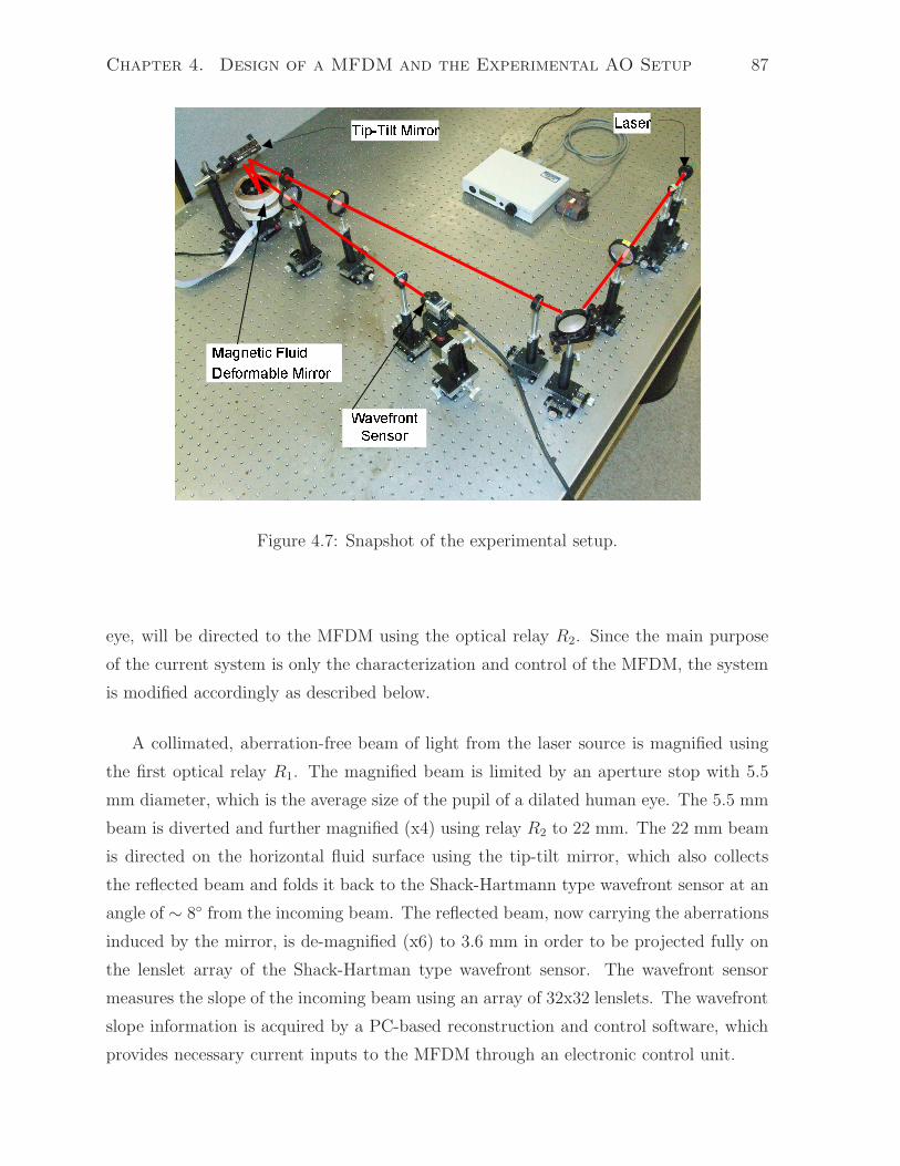
Chapter 4. Design of a MFDM and the Experimental AO Setup 87
Figure 4.7: Snapshot of the experimental setup.
eye, will be directed to the MFDM using the optical relay R2. Since the main purpose
of the current system is only the characterization and control of the MFDM, the system
is modified accordingly as described below.
A collimated, aberration-free beam of light from the laser source is magnified using
the first optical relay R1. The magnified beam is limited by an aperture stop with 5.5
mm diameter, which is the average size of the pupil of a dilated human eye. The 5.5 mm
beam is diverted and further magnified (x4) using relay R2 to 22 mm. The 22 mm beam
is directed on the horizontal fluid surface using the tip-tilt mirror, which also collects
the reflected beam and folds it back to the Shack-Hartmann type wavefront sensor at an
angle of ∼ 8 from the incoming beam. The reflected beam, now carrying the aberrations
induced by the mirror, is de-magnified (x6) to 3.6 mm in order to be projected fully on
the lenslet array of the Shack-Hartman type wavefront sensor. The wavefront sensor
measures the slope of the incoming beam using an array of 32x32 lenslets. The wavefront
slope information is acquired by a PC-based reconstruction and control software, which
provides necessary current inputs to the MFDM through an electronic control unit.

Chapter 4. Design of a MFDM and the Experimental AO Setup 88
!""
#""$%%&' ("")*$+%
+% ! ,
Figure 4.8: Schematic layout of the experimental setup. The components shown in the
blue color (dashed lines) are to be incorporated later. The subscripted letters L, M, R
and BS indicate a lens, mirror, relay and beam-splitter, respectively. All dimensions are
in mm.
4.2.2 Description of the Main Components
Important features of the main components of the system are described below.
Wavefront Sensor
The Shack-Hartmann type wavefront sensor (HASO 32 by Imagine Optic, Orsay, France)
comprises a 32x32 array of lenslets. The sensor has an aperture dimension of 3.6x3.6
mm backed by a CCD camera detector (Toshiba Teli CS8550i-01) and operates at a
maximum acquisition frequency of 30 Hz. The wavefront slope data, measured discretely
at the 32x32 sub-apertures of the wavefront sensor is acquired by a PCI frame-grabber
(Euresys Domino Alpha2 acquisition board) which provides an interface to a host PC.
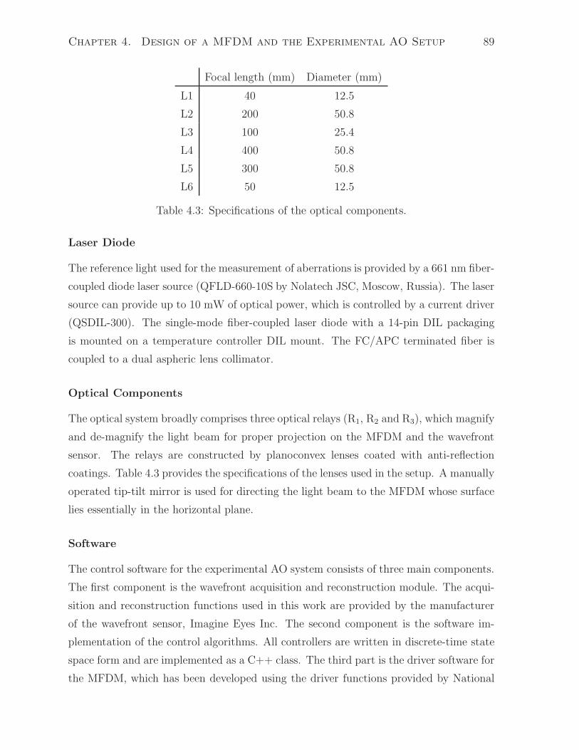
Chapter 4. Design of a MFDM and the Experimental AO Setup 89
Focal length (mm) Diameter (mm)
L1 40 12.5
L2 200 50.8
L3 100 25.4
L4 400 50.8
L5 300 50.8
L6 50 12.5
Table 4.3: Specifications of the optical components.
Laser Diode
The reference light used for the measurement of aberrations is provided by a 661 nm fiber-
coupled diode laser source (QFLD-660-10S by Nolatech JSC, Moscow, Russia). The laser
source can provide up to 10 mW of optical power, which is controlled by a current driver
(QSDIL-300). The single-mode fiber-coupled laser diode with a 14-pin DIL packaging
is mounted on a temperature controller DIL mount. The FC/APC terminated fiber is
coupled to a dual aspheric lens collimator.
Optical Components
The optical system broadly comprises three optical relays (R1, R2 and R3), which magnify
and de-magnify the light beam for proper projection on the MFDM and the wavefront
sensor. The relays are constructed by planoconvex lenses coated with anti-reflection
coatings. Table 4.3 provides the specifications of the lenses used in the setup. A manually
operated tip-tilt mirror is used for directing the light beam to the MFDM whose surface
lies essentially in the horizontal plane.
Software
The control software for the experimental AO system consists of three main components.
The first component is the wavefront acquisition and reconstruction module. The acqui-
sition and reconstruction functions used in this work are provided by the manufacturer
of the wavefront sensor, Imagine Eyes Inc. The second component is the software im-
plementation of the control algorithms. All controllers are written in discrete-time state
space form and are implemented as a C++ class. The third part is the driver software for
the MFDM, which has been developed using the driver functions provided by National

Chapter 4. Design of a MFDM and the Experimental AO Setup 90
Instruments. The whole system is integrated using a C++ console application accessing
the three components in a closed-loop. A single PC, using a 4200+ AMD Athlon 64X2
Dual Core processor with 2 Gigabytes of RAM, centrally controls the sensor acquisition,
controller data processing and MFDM actuation.
Miscellanea
Uniformity of the Initial Surface The Helmholtz coil used in the prototype MFDM
has a uniformity of less than 0.1% as measured at 20 mm diameter. Although small in
magnitude, the non-uniformity of the magnetic field of the Helmholtz coil does produce
a curvature in the initial surface of the fluid. Moreover, any misalignment in the vertical
axis of the Helmholtz coil and the gravitational vector, as well as the imperfections in
the optical components, result in a non-flat initial wavefront surface as measured by the
wavefront sensor. Though the tilt and the curvature in the initial surface measurements
can be minized by properly adjusting the tip-tilt mirror ( see Figure 4.7) and the position
of the wavefront sensor, some deformations of the initially measured wavefront surface
remain uncorrected. Generally these initial imperfections in the system are eliminated
by pre-setting the actuators, which ensures a planar initial wavefront surface.
Effect of the Earth’s Magnetic Field The effects of the earth’s magnetic field have
been ignored. For our experimental setup with the miniature coil strength bz ≈ 0.25
mT and earth’s magnetic field ≈ 0.055 mT (Toronto, Canada [112]) the approximation
is valid. However, with any smaller coils the effects of the earth’s magnetic field may
be significant. Under such circumstances the vertical component of the earth’s magnetic
field can be directly added to the uniform field of the Helmholtz coil without affecting
the validity of the model.
4.3 Summary
In this chapter, the design of the prototype MFDM and the experimental AO setup has
been described. The novel conceptual design change prompted by the findings of the
analytical work presented in chapter 3 is implemented in the design of the prototype
MFMD by using a Helmholtz coil. A description of the design requirements and the
design variables of a MFDM is presented. The detailed design of the prototype MFDM
is described. An adaptive optics setup is designed and assembled. The details of the

Chapter 4. Design of a MFDM and the Experimental AO Setup 91
layout of the experimental setup and the description of the components used in the setup
are presented. The prototype mirror and the experimental setup are designed to be used
to validate the analytical model of the mirror and to evaluate the performance of the
controllers presented in the next chapter.

Chapter 5
Control System Design
This chapter presents three control algorithms that can be used to control a magnetic
fluid deformable mirror in a closed-loop adaptive optics system. Firstly, a decentral-
ized proportional plus integral (PI) controller designed based on decoupling the plant
model at DC is presented. This is a commonly used type of controllers in adaptive
optics systems. The capabilities and limitations of this type of controllers are investi-
gated. To overcome stability robustness issues in the first algorithm, a decentralized
robust proportional-integral-derivative (PID) controller with DC decoupling is then pre-
sented. The controller is designed based on a decoupled nominal dynamic model of
the plant. To account for the modeling errors in the decoupled plant model, a robust
PID controller design problem is formulated and solved using algorithms based on linear
matrix inequalities (LMI). The two control algorithms mentioned above provide good
performance in removing static or very slowly changing aberrations, but have limited
capabilities in dealing with fast-changing aberrations. To overcome this limitation, an
H∞ multivariable controller that is designed using the mixed-sensitivity H∞ technique
is presented. This controller ensures that the mirror can cancel the unknown dynamic
wavefront aberrations that fall within the band of frequencies commonly seen in ocu-
lar wavefront aberrations. Simulation results showing the performance of the designed
closed-loop system in canceling the distortions in the aberrated wavefront will be pre-
sented. Results of laboratory experiments conducted to test the control algorithms on
the AO setup described in chapter 4 are presented in the following chapter.
Notation: For a given system Σ, Σ(s) and Σ(z) denote, respectively, the continuous
and discrete-time transfer functions of the system, and Σ :[
A B
C D
]
refers to a state-
space realization of the system Σ. In the block diagrams presented in this chapter, any
92

Chapter 5. Control System Design 93
given signal is represented using the same symbol in the time domain, Laplace domain,
and the z domain.
5.1 Description of the Closed-loop System
The control system is one of the three major components of an AO system; the other two
being the wavefront sensor and the wavefront corrector. In a closed-loop AO system, the
function of the control system is to utilize the wavefront aberration measurements made
by the wavefront sensor and generate a set of actuator commands. The latter are then
applied to remove the distortions in the aberrated wavefront.
Figure 5.1 shows the block diagram of a typical closed-loop AO system. The system
makes use of a wavefront corrector (WFC) where u is the vector of control currents
applied to the WFC, ζ is the resulting shape of the deformable mirror surface, ζaberrated
is the shape of the aberrated wavefront incident on the mirror surface and ζs is the shape
of the wavefront reflected from the mirror and sensed by the wavefront sensor. The
mirror surface shape and the incoming aberrated wavefront interact in such a way that
the sensed wavefront shape ζs can be written as [139]:
ζs = ζaberrated − 2ζ (5.1)
The sensor block in Figure 5.1 refers to both the wavefront sensor and the reconstruc-
tion algorithm that runs inside the control computer. The sensor samples the residual
wavefront ζs at discrete locations - using an array of lenslets in the case of the Shack-
Hartmann wavefront sensor. Though the sampled data can be directly utilized in control
computations, it is generally more helpful to reconstruct the shape of the sensed wave-
front surface. The reconstructed shape can then be used to interpolate the wavefront
surface displacements at any location in the pupil. The wavefront shape, expressed as
a vector zs ∈ RM of M discrete displacements, is provided to the controller K, which
computes the actuator commands u ∈ RL to be applied to the array of L input actuators.
Typically, the actuator commands are computed such that their application results in
the cancellation of the distortions present in the aberrated wavefront i.e., the residual
wavefront measurements ζs approach zero.
To simplify the implementation of the closed loop system and the testing of the perfor-
mance of the proposed control algorithms, an equivalent closed loop system configuration
is considered in Figure 5.2(a). In this configuration, a laser beam with a planar wavefront

Chapter 5. Control System Design 94
szP S
aberratedζ
ζ sζu- 22ζ
Figure 5.1: Block diagram of a typical closed-loop adaptive optics system.
szP S
2sζ ζ= −u.er2−
ζ
(a)
syP S
2ζu/er2
ζ
(b)
Figure 5.2: (a) Block diagram of the modified closed-loop adaptive optics system. (b)
Equivalent negative feedback block diagram representation.

Chapter 5. Control System Design 95
is directed towards the deformable mirror with surface shape ζ . The wavefront shape in
the reflected beam is given by ζs = −2ζ . The wavefront shape is measured by the wave-
front sensor and is reconstructed inside the control computer. The measured wavefront
shape vector zs ∈ RM is sampled from the reconstructed shape. The measured wavefront
shape is then added, inside the control computer, to a hypothetical aberrated wavefront
shape. The hypothetical aberrated wavefront shape is sampled at the same locations at
which the measured wavefront shape vector ys is computed from the reconstructed shape.
An equivalent block diagram representation that is consistent with the representation of
negative feedback control systems is shown in Figure 5.2(b), where ys = −zs. Denoting
the sampled aberrated wavefront shape as r ∈ RM , the wavefront shape error e ∈ R
M
fed to the controller K can be written as:
e = r − ys (5.2)
In this configuration, the controller K is required to provide input commands u such that
the magnitude of the wavefront shape error e is minimized. A statement of the control
problem addressed in this thesis is given as follows:
Problem Statement:
With respect to the feedback system shown in Figure 5.2(b), it is desired to
design a controller K to provide input currents u such that the signal ys (rep-
resenting twice the shape of the MFDM surface) tracks the reference wavefront
shape signal r (representing the aberrated wavefront shape ζaberrated).
The main advantage in considering the feedback system shown in Figure 5.2(b) is that
any aberrated wavefront shape can be easily considered and analytically generated as
opposed to physically generating it as in the closed loop system shown in Figure 5.1.
5.1.1 The Plant Model
In the following, the analytical model of the MFDM presented in chapter 3 is used for the
development of controllers to control the mirror surface shape in the closed-loop system
shown in Figure 5.2(b). As shown in Figure 5.2(b), an augmented plant G is defined
and includes the WFC, a model of the optical interaction between the incident beam
and the deformable mirror, and the wavefront sensor. Using the notation given at the

Chapter 5. Control System Design 96
beginning of this chapter, the WFC P will be represented by the transfer function P(s)
and a corresponding state-space realization P :
[
A B
C 0
]
, where the system matrices
A, B and C are obtained from the mirror model (3.90) and are given in Appendix B.
As mentioned earlier, the magnitude of the wavefront shape as measured by the sensor
is twice the magnitude of the mirror shape. The sensor also introduces a delay in the
closed-loop. Therefore, the augmented plant G is defined as having a transfer function
G(s) = 2e−TssP(s), where Ts is the sensor delay. By approximating the time delay
transfer function e−Tss using a rational transfer function, an approximate model of the
augmented plant G can be given in state-space form as:
x = Agx + Bgu
ys = Cgx(5.3)
where x ∈ RNG is the vector of state variables, ys ∈ R
M is the vector of sensor outputs,
Ag ∈ RNG×NG , Bg ∈ R
NG×L and Cg ∈ RM×NG are the system matrices with appropriate
dimensions.
The discretized version of the augmented plant model G can be obtained using the
discrete-time model (3.91) of the WFC. The WFC is represented by discrete-time trans-
fer function P(z) and a corresponding state-space realization P :
[
Ad Bd
Cd 0
]
, where
Ad, Bd and C are given in (3.91). The discrete-time model of the augmented plant G is
represented using the transfer function G(z) = 21zP(z) and a corresponding state-space
modelx(k + 1) =Agdx(k) + Bgdu(k)
ys(k) =Cgx(k)(5.4)
where Agd and Bgd are matrices with appropriate dimensions.
5.1.2 Decoupling of the Input-Output Channels
Given the low frequency content of the aberrations of interest, it is desired in this section
to investigate the decoupling of the plant model at DC. Decoupling the plant model
significantly facilitates the controller design for the AO system, as the problem of MIMO
controller design can be reformulated as that of designing a set of SISO controllers. The
developed DC decoupled models are used in the design of decentralized PI and PID
controllers presented later in this chapter.

Chapter 5. Control System Design 97
0
5
10
15
From: In(1)
To:
Out
(1)
0
5
10
15
To:
Out
(2)
10−1
100
101
102
0
5
10
15
To:
Out
(3)
From: In(2)
10−1
100
101
102
From: In(3)
10−1
100
101
102
Frequency (rad/sec)
Mag
nitu
de (
abs)
Figure 5.3: Bode magnitude plots corresponding to three selected input-output channels
in the augmented plant model G.
As predicted by the analytical model (3.90), and experimentally validated in the
following chapter, the mirror surface shape generated by the magnetic field of a single
electromagnetic coil features a Gaussian profile, with the peak surface deflections ob-
tained immediately above the center of the coil. This feature of the MFDM allows the
augmented plant G to be decoupled and represented as a collection of SISO systems
since the coupling among the different input-output channels can be minimized by ap-
propriately choosing the location of the output points. For the 19-input channel system
as described in section 4.2, 19 output points in the reconstructed wavefront shape are
chosen such that each of the output points corresponds to the location of an input coil as
seen in the optical pupil. This arrangement ensures that each output point is influenced
maximally by one input coil only, i.e. the one corresponding to its own locations, while
the effect of the other inputs is significantly small. The decoupling effect can be clearly
observed from the Bode magnitude plot of the augmented plant G as shown in Figure
5.3, where magnitudes in the plots on the leading diagonal are significantly higher than
those placed off-diagonal. The figure shows the Bode plots for three selected channels
(#1, 2 and 10 as marked in Figure 4.4) only.
Chapter 5. Control System Design 98
Although the right choice of input-output points does produce the desired decoupling
effect, the system is still not fully decoupled. For example, the coupling between the
adjacent output points (1 and 2, for instance) is of the order of 20% (i.e., the magnitude
of the wavefront measured at the output point 2 due to an input applied at coil 1 is
approximately 0.2 times the magnitude of the wavefront measured at the output 1 due
to the input applied at coil 1). Therefore, some means of further reducing the coupling
effect are still needed.
A decoupling technique, which utilizes the DC gain of the MIMO system, is considered
in the following to minimize the remaining coupling effects. This approach is motivated
by the observation that the magnitude responses shown in Figure 5.3 remain constant over
a range of low frequencies. This implies that the augmented plant G can be considered
as a static system in this range of frequencies. Since a static MIMO system can be
fully decoupled using the DC gain of the system [113], this property of the plant G
is exploited to further improve the decoupling effect produced by the choice of output
points as described above.
The DC gain of the augmented plant G(s) (5.3) can be obtained as:
G0 = G(0) = −CgA−1g Bg (5.5)
For frequencies ω < ω0 over which the gains of all the channels of G(s) remain constant,
the following relationship holds:
∣∣G(jω)G−1
0
∣∣ ≈ I for ω < ω0 (5.6)
where I is an identity matrix. It follows from (5.6) that for ω < ω0 the system G given
by
G(s) = G(s)G−10 (5.7)
is a decoupled system with a unit DC gain associated with each of the decoupled channels.
This decoupling effect can be incorporated in a closed loop system by simply cascading
the gain G−10 with the plant G as shown in Figure 5.4. The decoupling effect can be more
clearly observed in the magnitude response plots for the system G given in Figure 5.5. It
is obvious that the system is significantly decoupled in the low frequency range ω < 12
rad/s. Note that the magnitude plots on the leading diagonal only have significant values.

Chapter 5. Control System Design 99
sy′uer
G
uG1
0−G
0K
Figure 5.4: Block diagram of the closed-loop system using DC gain matrix.
0
0.5
1From: In(1)
To:
Out
(1)
0
0.5
1
To:
Out
(2)
10−2
10−1
100
101
102
0
0.5
1
To:
Out
(3)
From: In(2)
10−2
10−1
100
101
102
From: In(3)
10−2
10−1
100
101
102
Frequency (rad/sec)
Mag
nitu
de (
abs)
Figure 5.5: Bode magnitude plots of the decoupled plant model.

Chapter 5. Control System Design 100
For the discrete-time model (5.4) of the augmented plant G, the DC gain remains
the same as given in (5.5), and can also be obtained using the system matrices of the
discrete-time model as:
G0 = Cg(I − Agd)−1Bgd (5.8)
Inserting the inverse of the DC gain matrix G0 before the augmented plant G in the
closed loop system, the discretized version of G can be obtained as:
G(z) = G(z)G−10 (5.9)
where
∣∣G(z)
∣∣ ≈ I for ω < ω0 (5.10)
A decoupled system can be treated as a collection of SISO systems that can be
controlled independently. For the system G, a decentralized type controller K can be
designed such that K = kI, where k is a SISO controller. Given K, the overall controller
K for the plant G can be written as:
K = G−10 K (5.11)
The decoupling approach presented in this section is used in the design of decentralized
PI and PID controllers for the AO system as discussed in the following two sections.
5.2 Decentralized PI Controller with DC Decoupling
Most of the existing AO systems make use of controllers designed based on a DC model
of the response of the reflected wavefront shape to the inputs applied to the wavefront
corrector. In the AO community, the DC model is commonly referred to as the influence
function matrix and is actually the DC gain of the augmented plant comprising the
wavefront corrector and the wavefront sensor. For the purpose of controller design in this
section, the closed-loop system block diagram is as shown in Figure 5.4, except that the
plant model G is replaced by its DC gain G0.
As mentioned in section 2.3.5, the major difficulty in controlling the conventional
MFDM arises from the nonlinear nature of the response of its deformable surface. A
clear manifestation of this difficulty has been the failure of the influence function based

Chapter 5. Control System Design 101
control algorithms [15, 18]. Now that the nonlinearity of the response of the MFDM has
been taken care of by modifying the design of the mirror, it is reasonable to expect that
controllers designed based on the DC-decoupled plant model should succeed in removing
the distortions in the aberrated wavefront, or at least do so with respect to the static
aberrations. In the following, a decentralized PI controller is designed and its performance
is evaluated through simulation studies.
5.2.1 Controller Design
Assuming the plant G(z) is represented by its DC model G0, it follows that
G(z) = I (5.12)
The resulting system is a decoupled system with unit gains in each of the decoupled
channels. For such a system, a decentralized type controller K can be designed such that
K = kI, where k is a scalar controller designed for the static plant (5.12). In this section,
and with aim of dealing mostly with static aberrations, a proportional plus integral (PI)
type controller is considered. The controller k is given by:
k(z) =(kp + ki)z − kp
z − 1(5.13)
where kp and ki are, respectively, the proportional and integral gains of the controller.
The controller gains can be obtained using any of the standard control design methods
[138]. Using the classical pole placement method the following parameters were obtained:
kp = 0.032, ki = 0.288. (5.14)
The overall controller K is given by G−10 kI obtained as kG−1
0 . The controller thus
obtained can be used to control the augmented plant G in the closed-loop system. Sim-
ulation results of the closed-loop system response are presented in the following section.
5.2.2 Simulation of the Closed-loop System
To evaluate the performance of the decentralized PI controller, typical static and dynamic
aberrated wavefront shapes are specified as reference signals r (see Figure 5.2). Each entry
in r is associated with a spatial location corresponding to the center of one of the 19 coils.

Chapter 5. Control System Design 102
The static reference wavefront shape considered in this simulation is given by:
ro = [2.0, 4.0, 5.0, 1.0, 5.5, 0.5, 3.5, 8.5, 6.0, 3.0, 2.5, 2.0, 3.0, 4.0,−2.0, ...
− 4.0,−5.0, 1.0, 6.0]T (5.15)
whereas the dynamic reference wavefront shape is given by:
r = r0 + [sin(fot+ φ1), ..., sin(fot+ φ19)]T (5.16)
where r0 is as in (5.15), fo is the frequency of the sinusoidally varying component of the
aberrated wavefront shape and φm, m = 1, 2, ..., 19, are the phases, chosen randomly such
that 0 < φm < π2. All the entries in r0 and r are expressed in micrometers. In (5.16), the
2µm peak-to-valley dynamic reference wavefront shape signals are superimposed on the
static off set ro to represent the aberrations in the eye, which almost always have a large
static component. These reference wavefront shapes will be utilized in the simulations of
all the controllers presented in this chapter and in the experimental results presented in
chapter 6.
Simulation results involving the static reference wavefront shape given in (5.15) are
shown in Figure 5.6. The time history of the wavefront shape measurements ys at the 19
output locations is shown in Figure 5.6(a). The corresponding reference wavefront shape
signals ro are shown as dashed lines. The control inputs as determined by the designed
controller are given in Figure 5.6(b). The root mean square (RMS) of the wavefront
shape error e computed for the 19 channels is given in Figure 5.6(c). As evident from the
simulated results, the output of the closed-loop system can successfully track the static
reference shape.
Figure 5.7 shows simulations results involving the dynamic reference shape given in
(5.16). The time history of the wavefront shape measurements ys is shown in Figure
5.7(a). For clarity the results for only selected channels (# 2, 4, 8 and 17) are shown
in the figure. The corresponding reference wavefront shape signals are shown as dashed
lines. The control inputs as determined by the designed controller are given in Figure
5.7(b). The RMS of the wavefront shape error e computed for the 19 channels is given
in Figure 5.7(c). As expected, the tracking capability of the closed-loop system is very
limited in this case.
The following important observations can be made from the simulation results pre-
sented above:
Chapter 5. Control System Design 103
• It was demonstrated that the PI controller designed based on a DC model (i.e. the
influence function) of the response of the WFC can be successfully used to control
the MFDMs developed according to the design modification proposed in this thesis.
• The decentralized PI controller asymptotically drives the wavefront shape error to
zero, when tracking the static reference wavefront shape signals. High performance
tracking of static reference signals remains a characteristic feature of the controllers
that have an integrator in their structure. The same was verified by the simulations
presented above.
• The performance of the decentralized PI controller in canceling dynamic wavefront
aberrations was found to be inadequate. The controller provides the desired track-
ing of the dynamic reference wavefront shape signals when the reference signals
change very slowly with time. But the performance of the closed-loop system dete-
riorates rapidly with the increasing frequency of the reference signals as illustrated
in Figure 5.7(a), which shows the results for the dynamic reference wavefront signals
(5.16) with 3 Hz frequency.
• An important closed-loop system stability issue is related to the fact that the PI
controller is designed based on the assumption that the augmented plant is a static
system. The MFDM exhibits significant dynamics even in the low frequency range,
which leads to stability robustness issues in the resulting closed loop system. This
latter issue is addressed in the following section.

Chapter 5. Control System Design 104
0 0.5 1 1.5 2 2.5 3−6
−4
−2
0
2
4
6
8
10
Time (s)
Wav
efro
nt S
hape
ys (
µm)
(a)
0 0.5 1 1.5 2 2.5 3−15
−10
−5
0
5
10
15
20
Time (s)
Con
trol
Cur
rent
s (m
A)
(b)
0 0.5 1 1.5 2 2.5 30
0.5
1
1.5
2
2.5
3
3.5
4
4.5
Time (s)
RM
S E
rror
(µm
)
(c)
Figure 5.6: Tracking of a static reference shape using the decentralized PI controller. (a)
Wavefront Shape. (b) Control Inputs. (c) RMS Error.
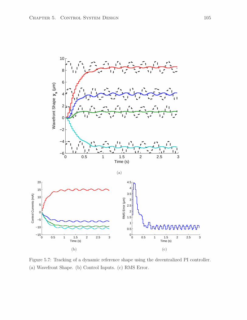
Chapter 5. Control System Design 105
0 0.5 1 1.5 2 2.5 3−6
−4
−2
0
2
4
6
8
10
Time (s)
Wav
efro
nt S
hape
ys (
µm)
(a)
0 0.5 1 1.5 2 2.5 3−15
−10
−5
0
5
10
15
20
Time (s)
Con
trol
Cur
rent
s (m
A)
(b)
0 0.5 1 1.5 2 2.5 30
0.5
1
1.5
2
2.5
3
3.5
4
4.5
Time (s)
RM
S E
rror
(µm
)
(c)
Figure 5.7: Tracking of a dynamic reference shape using the decentralized PI controller.
(a) Wavefront Shape. (b) Control Inputs. (c) RMS Error.

Chapter 5. Control System Design 106
5.3 Decentralized Robust PID Controller Design Based
on Linear Matrix Inequalities
5.3.1 Introduction
A decentralize PI controller was presented in the previous section. The controller was
designed based on the assumption that the augmented plant G can be considered to be
a static system represented by its DC gain G0. Therefore, the resulting DC decoupling
of the plant model, which is strictly valid for ω = 0 only, was assumed to be effective
for all operating frequencies. However, the approximation of the plant model by a static
model introduces modeling errors whose effects become more pronounced as the frequency
content of the reference inputs increases. These modeling errors also lead to stability
robustness problems in the resulting closed loop system. In order to minimize the effect
of these uncertainties, a robust PID controller with a decentralized structure is designed in
this section. Uncertainties in the plant model are taken into account during the controller
design process. The problem of designing the robust decentralized PID controller is
formulated as an optimization problem, and the controller gains are determined by solving
a set of linear matrix inequalities (LMIs).
5.3.2 Controller Design
The system G in (5.7) can be represented using the following transfer matrix:
G(s) =
g11(s) g12(s) · · · g1L(s)
g21(s) g22(s) · · · g2L(s)...
.... . .
...
gM1(s) gM2(s) · · · gML(s)
(5.17)
As indicated by the selected Bode magnitude plots shown in Figure 5.5, the diagonal
entries represent the most significant entries in G(s), whereas the contribution of the
other entries is much less significant. Moreover, the diagonal entries in G(s) are all
similar. Hence, these entries can all be represented using the same function g(s), and

Chapter 5. Control System Design 107
−20
−15
−10
−5
0
5
Mag
nitu
de (
dB)
10−1
100
101
102
−270
−180
−90
0
Pha
se (
deg)
Frequency (rad/sec)
Typical diagonal element in G(s)
g(s)
Figure 5.8: Bode plots g(s) and that of a typical diagonal entry in G(s).
therefore,
G(s) =
g(s) g12(s) · · · g1L(s)
g21(s) g(s) · · · g2L(s)...
.... . .
...
gM1(s) gM2(s) · · · g(s)
(5.18)
The function g(s) can be approximated using a dynamic model given by
g(s) = Pl(s)Sl(s) (5.19)
where Pl(s) = 7(s+194.3)(s+20)(s+68)
approximates each of the diagonal entries in G as a second
order system, assuming there is no time delay, and Sl(s) = 12−6Tss+(Tss)2
12+6Tss+(Tss)2is the Pade
approximation of the sensor delay transfer function e−Tss [132], with TS = 0.0345 sec.
Figure 5.8 shows a comparison of the Bode plots of g(s) and one of the diagonal entries
in G(s). The comparison indicates that g(s) provides an accurate representation of the
diagonal entries in G(s).
Using (5.19), the system G in (5.7) can be represented as:
G(s) = g(s)I + (G − g(s)I) (5.20)
= g(s)I + ∆(s) (5.21)

Chapter 5. Control System Design 108
sy′u( )PID s
1er ′y
∆
( ) ( ) ( )s s g s∆ = −G I
( )sG
( )sWe2 r
y3
( )w s∆ I
( )g s I
Figure 5.9: Block diagram of the closed-loop system with the uncertain plant model.
where ∆(s) is considered a modeling uncertainty. In the following, a robust decentralized
PID controller KPID, which takes into account the modeling uncertainty ∆(s), will be
designed for the decoupled system given by g(s)I. The controller KPID has a decentral-
ized structure and is given by KPID = kPIDI, where kPID is a single channel controller.
A block diagram of the closed-loop system is shown in Figure 5.9.
To simplify the design of the PID controller, the uncertainty term ∆(s) is approxi-
mated as
∆(s) = w∆(s)∆ (5.22)
where ∆ ∈ RN×N is such that every entry δij, i = 1, 2, ...,M, j = 1, 2, ..., L, in ∆ satisfies
−κ ≤ δij ≤ κ, and where κ can be determined experimentally. In (5.22), w∆(s) is a high
pass filter since the uncertainty is zero at ω = 0 and increases with increasing frequency.
In order to eliminate any high frequency component in the error signal, the filter matrix
W = w(s)I, where w(s) is a low pass filter, is introduced in the closed loop system.
For the purpose of stability robustness analysis, the signal r is set to zero, and the
closed loop system block diagram is redrawn as shown in Figure 5.10, where∑
is the
system with input r and output y. The system∑
is given by
∑
= w∆WKPIDS (5.23)
where S is the sensitivity function given by
S =(I + gKPIDW)−1 (5.24)
= (1 + gkPIDw)−1I (5.25)
With KPID = kPIDI and W = wI, it follows that

Chapter 5. Control System Design 10945y
6r
Figure 5.10: Redrawn block diagram of the closed-loop system.
S = SI (5.26)
where
S = (1 + gkPIDw)−1 (5.27)
Therefore the system∑
can be expressed as
∑
= w∆wkPIDSI (5.28)
Assuming∑
is stable, the internal stability of the closed loop shown in Figure 5.10 is
satisfied if [137]
‖∆‖∥∥∥
∑∥∥∥∞< 1 (5.29)
which is equivalent to∥∥∥
∑∥∥∥∞< ‖∆‖−1 (5.30)
Let JM ∈ RM×M be such that all its entries are equal to one. Then, ‖∆‖ ≤ κσmax(JM),
where σmax() denotes the maximum singular value. Since ‖∆‖−1 ≥ 1κσmax(JM )
, it follows
that (5.30) is satisfied if∥∥∥
∑∥∥∥∞<
1
γ(5.31)
where γ denotes κσmax(JM).
Since∑
= w∆wkPIDSI, it follows that ‖∑‖∞ = ‖w∆wkPIDS‖∞. Hence the condi-
tion (5.31) is equivalent to
‖w∆wkPIDS‖∞ <1
γ(5.32)
The stability robustness problem is therefore transformed into a PID controller design
problem such that ‖w∆wkPIDS‖∞ < 1γ.
The transfer function w∆wkPIDS corresponds to the transfer function of any of the
decoupled channels in the system∑
. For a multivariable signal v, let vi denote the ith
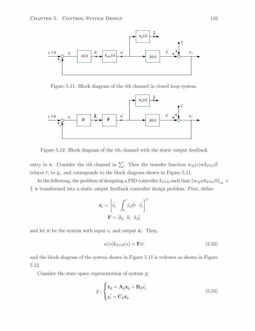
Chapter 5. Control System Design 110
siyiu′
( )PIDk sie0ir = iy′ie7 ir
iy8
( )w s∆
( )g s( )w s
Figure 5.11: Block diagram of the ith channel in closed loop system.
siyiu′
Fie0ir = iy′ˆ ie
ir
iy9
( )w s∆
( )g sw
Figure 5.12: Block diagram of the ith channel with the static output feedback
entry in v. Consider the ith channel in∑
. Then the transfer function w∆(s)wkPIDS
relates ri to yi, and corresponds to the block diagram shown in Figure 5.11.
In the following, the problem of designing a PID controller kPID such that ‖w∆wkPIDS‖∞ <1γ
is transformed into a static output feedback controller design problem. First, define
ei =
[
ei
∫ t
0
eidτ ˙ei
]T
F = [kp ki kd]
and let w be the system with input ei and output ei. Then,
w(s)kPID(s) = Fw (5.33)
and the block diagram of the system shown in Figure 5.11 is redrawn as shown in Figure
5.12.
Consider the state space representation of system g;
g :
xg = Agxg + Bgu′
i
y′
i = Cgxg
(5.34)

Chapter 5. Control System Design 111
where xg ∈ Rng is the vector of state variables, u
′
i ∈ R, y′
i ∈ R, Ag ∈ Rng×ng , Bg ∈ R
ng
and Cg ∈ R1×ng . Similarly, w(s) can be represented as
w :
xw = Awxw + Bwei
ei = Cwxw
(5.35)
where xw ∈ Rnw is the vector of state variables, ei ∈ R, ei ∈ R, Aw ∈ R
nw×nw , Bw ∈ Rnw
and Cw ∈ R1×nw . The system w∆(s) is given by
w∆ :
x∆ = A∆x∆ + B∆u′
i
yi = C∆x∆
(5.36)
where x∆ ∈ Rn∆ is the vector of state variables, yi ∈ R, A∆ ∈ R
n∆×n∆ , B∆ ∈ Rn∆ and
C∆ ∈ R1×n∆ .
With ri = 0, ei can be written as:
ei = − (y′
i + ri)
= −Cgxg − ri (5.37)
The control signal generated in the ith channel is given by
u′
i = kpei + ki
∫ t
0
eidτ + kd ˙ei (5.38)
where kp, ki , kd ∈ R are the parameters to be designed. Let zi =[zTi1 zTi2 zTi3 z
Ti4
]Tbe a
vector of new state variables defined as
zi1 = xg, zi2 = xw, zi3 = x∆ and zi4 =
∫ t
0
eidτ
Define new output variables
ei1 = ei =[
0 Cw 0 0]
zi
ei2 =
∫ t
0
eidτ =[
0 0 0 1]
zi
ei3 = ˙ei =[
−CwBwCg CwAw 0 0]
zi −CwBwri
ei = [ei1 ei2 ei3]T
which gives
ei = Cyzi + Dyri

Chapter 5. Control System Design 112
F
iol
: iy;
ieiu′ir
Figure 5.13: Block diagram of the closed-loop system with the static output feedback
controller F.
where
Cy =
0 Cw 0 0
0 0 0 1
−CwBwCg CwAw 0 0
, Dy =
0
0
−CwBw
The block diagram shown in Figure 5.12 can then be represented as shown in Figure
5.13, where the system∑i
ol can be represented as follows:
∑i
ol:
zi = Azi + B1ri + B2u′
i
yi = Cyzi
ei = Cyzi + Dyri
(5.39)
where
A =
Ag 0 0 0
−BwCg Aw 0 0
0 0 A∆ 0
0 Cw 0 0
,B1 =
0
−Bw
0
0
,B2 =
Bg
0
B∆
0
,Cy =[
0 0 C∆ 0]
The control signal given by (5.38) can now be considered to be the output of a static
output feedback controller since:
u′
i = Fei (5.40)
The problem of designing the robust PID controller is then transformed to that of
designing a static output feedback controller for the system (5.39) such that the constraint
(5.32) is satisfied. Using the static output feedback controller F given in (5.40), the state
space representation for the resulting closed-loop system is given by:
∑i
cl:
zi = (A + B2FCy) zi + (B1 + B2FDy) ri
yi = Cyzi
(5.41)

Chapter 5. Control System Design 113
For the closed-loop system (5.41), based on the Bounded Real Lemma [114], the con-
straint (5.32) is satisfied if and only if there exists a positive definite matrix P such
that
P (A + B2FCy)T + (A + B2FCy)P (B1 + B2FDy) PCT
y
(B1 + B2FDy)T − 1
γ2 I 0
CyP 0 −I
< 0. (5.42)
Since the above matrix inequality is nonlinear in the unknown parameters P and F, it
cannot be solved directly using LMI solvers. In the following, an algorithm based on [114]
is used to obtain a solution for (5.42) by iteratively solving a set of properly formulated
linear matrix inequalities. Using the Schur complement, inequality (5.42) can be written
as
P (A + B2FCy)T + (A + B2FCy)P
+ γ2 (B1 + B2FDy) (B1 + B2FDy)T + PCT
yCyP < 0 (5.43)
γ−1 > 0 (5.44)
Inequality (5.43) is satisfied if
PAT + AP −PCTyCyP +
(B2F + PCT
y
) (B2F + PCT
y
)T
+ γ2 (B1 + B2FDy) (B1 + B2FDy)T + PCT
yCyP < 0 (5.45)
Since for any X > 0 and P > 0
PCTyCyP ≥ XCT
yCyP + PCTyCyX − XCT
yCyX (5.46)
the inequality (5.45) is satisfied if
PAT + AP −XCTyCyP − PCT
yCyX + XCTyCyX +
(B2F + PCT
y
) (B2F + PCT
y
)T
+ γ2 (B1 + B2FDy) (B1 + B2FDy)T + PCT
yCyP < 0 (5.47)
Let α ≥ 0. Then a sufficient condition for (5.47) to be satisfied is
PAT +AP−αP−XCTy CyP−PCT
yCyX+XCTy CyX+
(B2F + PCT
y
) (B2F + PCT
y
)T
+ γ2 (B1 + B2FDy) (B1 + B2FDy)T + PCT
yCyP < 0 (5.48)

Chapter 5. Control System Design 114
Let Ψ = PAT +AP−αP−XCTyCyP−PCT
yCyX+XCTyCyX. Then (5.48) and (5.44)
are equivalent to
Ψ (B1 + B2FDy) PCTy B2F + PCT
y
(B1 + B2FDy)T − 1
γ2 I 0 0
CyP 0 −I 0(B2F + PCT
y
)T0 0 −I
< 0. (5.49)
In the following, an iterative LMI algorithm will be used to solve the above inequality.
Algorithm:
Step 1. Select Q > 0, and solve P > 0 from the following algebraic Riccati equation:
PAT + AP − PCTyCyP + Q = 0
Set i = 1 and Xi = P.
Step 2. Solve the following optimization problem for Pi, F and αi.
OP1: Minimize αi subject to the following LMI constraints
Ψ (B1 + B2FDy) PiCTy B2F + PiC
Ty
(B1 + B2FDy)T − 1
γ2 I 0 0
CyPi 0 −I 0(B2F + PiC
Ty
)T0 0 −I
< 0. (5.50)
Pi > 0 (5.51)
where Ψ = PiAT + APi−αPi−XiC
TyCyPi−PiC
TyCyXi +XiC
TyCyXi . Denote by α∗
i
the minimized value of αi.
Step 3. If α∗i ≤ 0, the resulting F satisfies the robust stability condition (5.32). Stop.
Step 4. Solve the following optimization problem for the unknowns Pi and F.
OP2: Minimize trace(Pi) subject to the LMI constraints (5.50) and (5.51) with
αi = α∗i . Denote by P∗
i the matrix Pi that minimizes trace(Pi).

Chapter 5. Control System Design 115
Step 5. If ‖Xi − P∗i ‖ < δ, a prescribed tolerance, go to step 6. Else set i = i + 1 and
Xi = P∗i−1, then go to step 2.
Step 6. Try a different Q in step 2 and run the algorithm again. Else, it may be
concluded that a solution F that satisfies the robust stability condition (5.32) could not
be found.
5.3.3 Simulation of the Closed-loop System
Using the algorithm described above a controller is designed for the system G(5.7). In
the controller design process, the low pass filter w1(s) is selected as
w(s) =1
0.006944s2 + 0.1179s+ 1(5.52)
For the 19-input-19-output system, based on experimental analysis, the uncertainty
bound κ = 0.2, which yields ‖∆‖ ≤ 0.2 × 19 = 3.8. The uncertainty weight function is
selected as
w∆ =s
s+ 10(5.53)
Using these parameters, the above algorithm provides the following PID controller
gains
kp = 0.30, ki = 0.26, kd = 0.65 (5.54)
Using (5.54), the controller kPID for each channel can be obtained as
kPID = kp + ki1
s+ kds (5.55)
which gives
K = KPID = kPIDI (5.56)
Using (5.56) in (5.11), the overall controller K can be obtained as
K = kPIDG−10 (5.57)
A closed-loop system comprising the augmented plant model G and the decentralized
PID controller (5.57) was simulated in order to determine the ability of the closed-loop
system to track the reference wavefront shapes signals. The results of the simulations
are as follows:

Chapter 5. Control System Design 116
0 0.5 1 1.5 2 2.5 3−6
−4
−2
0
2
4
6
8
10
Time (s)
Wav
efro
nt S
hape
ys (
µm)
(a)
0 0.5 1 1.5 2 2.5 3−15
−10
−5
0
5
10
15
20
Time (s)
Con
trol
Cur
rent
s (m
A)
(b)
0 0.5 1 1.5 2 2.5 30
0.5
1
1.5
2
2.5
3
3.5
4
4.5
Time (s)
RM
S E
rror
(µm
)
(c)
Figure 5.14: Tracking of a static reference shape using decentralized PID controller. (a)
Wavefront Shape. (b) Control Inputs. (c) RMS Error.

Chapter 5. Control System Design 117
Figure 5.14 shows the results of simulations where the closed-loop system is required
to track the static shape defined by (5.15). Figure 5.14(a) shows the time history of
the wavefront shape measurements ys at the 19 output locations. The corresponding
reference wavefront shape signals are shown as dashed lines. The control inputs as deter-
mined by the designed controller are given in Figure 5.14(b). The RMS of the wavefront
shape error e computed for the 19 channels is given in Figure 5.14(c). The output of
the closed-loop system was found to converge successfully to the desired reference shape
in less than 1 s. Note that the RMS error asymptotically approaches zero, which is the
characteristic feature of controllers with an integrator.
Figure 5.14(a) shows the results of simulations where the closed-loop system is re-
quired to track the dynamic reference wavefront shape signals specified in (5.16). Figure
5.15(a) shows the time history of the wavefront shape measurements ys at selected lo-
cations (# 2, 4, 8 and 17). The control inputs are given in Figure 5.15(b). As can
be observed from the figure, the controller manages to drive the wavefront shape ys
to the static off-set values of the reference signals. However, there exists a phase dif-
ference between the reference wavefront shape signals and the corresponding wavefront
shape measurements ys, which results in a relatively large RMS error as shown in Figure
5.15(c).
The closed-loop system based on the PID controller described above performs satis-
factorily in tracking slowly changing reference shapes. The integrator in the structure of
this type of controllers ensures that the error in tracking a constant reference shape is
driven to zero asymptotically. When tracking a dynamic reference wavefront shape, the
output of the closed loop system lags the reference wavefront shape signal, resulting in
significant tracking errors.

Chapter 5. Control System Design 118
0 0.5 1 1.5 2 2.5 3−6
−4
−2
0
2
4
6
8
10
Time (s)
Sur
face
Def
lect
ions
(µm
)
(a)
0 0.5 1 1.5 2 2.5 3−15
−10
−5
0
5
10
15
20
Time (s)
Con
trol
Cur
rent
s (m
A)
(b)
0 0.5 1 1.5 2 2.5 30
0.5
1
1.5
2
2.5
3
3.5
4
4.5
Time (s)
RM
S E
rror
(µm
)
(c)
Figure 5.15: Tracking of a dynamic reference shape using decentralized PID controller.
(a) Wavefront Shape. (b) Control Inputs. (c) RMS Error.

Chapter 5. Control System Design 119
syerrW
eW
∞K1
z
z −I
u
uWe<
G
u=
Figure 5.16: Closed-loop system structure for mixed sensitivity minimization.
5.4 Mixed Sensitivity H∞ Controller Design
5.4.1 Introduction
An advanced controller that guarantees satisfactory performance over the expected fre-
quency range of ocular aberrations is presented in this section. The controller is designed
to provide optimal H∞ performance in tracking the desired wavefront shapes using the
MFDM. A mixed sensitivity H∞ design approach is used, which not only ensures optimal
performance in tracking the desires wavefront shapes but also limits the magnitude of the
control currents. The difficulties faced in using PI and PID controllers presented above
are satisfactorily dealt with using the controller presented in this section.
5.4.2 Problem Formulation
The closed-loop system used in the controller design process is shown in Figure 5.16,
where G is the discretized augmented plant model (5.4) representing the WFC and the
sensor.
The diagonal matrices We, Wu and Wr are the weighting functions which guide
the optimization process employed to search for the optimal controller parameters. The
weighting function We = weI, where we is a scalar low pass filter, is used to shape
the sensitivity function S, i.e. the transfer function from the reference signal r to the
performance variable e. Since the successful tracking of the reference r by the closed-loop
system is implied in minimization of the performance variable e, it can be achieved if
the maximum singular value of S is made small over the desired frequency range. The
low pass filter we is selected such that the weighted sensitivity function WeS is limited

Chapter 5. Control System Design 120
to the desired frequency range.
The weighting function Wu = wuI, where wu is a scalar high pass filter with a
crossover frequency approximately equal to the desired closed loop bandwidth. The
weighting function is used to limit the controller output. It also contributes toward the
robustness of the closed-loop system by minimizing the controller output in the frequency
range beyond the desired closed-loop bandwidth [137].
The weighting function Wr = wrI, where wr is a scalar low pass filter, is used in
the controller design process to penalize the controller in the frequency range beyond the
bandwidth of the expected wavefront shapes to be tracked.
The integrator shown in Figure 5.16 has been introduced to ensure that the error in
tracking the static reference signals is driven to zero. With the integrator block included,
the overall controller becomes
K = K∞z
z − 1I (5.58)
where K∞ is the H∞ controller.
With the structure of the closed-loop system selected as described above, the mixed
sensitivity H∞ controller design problem can be formulated as follows:
minK
∥∥∥∥∥
[
WeSWr
WuKSWr
]∥∥∥∥∥∞
(5.59)
where WeSWr and WuKSWr are the transfer functions from r to e and from r to u,
respectively.
Suppose the state space representation of Wr, We, Wu is Wr :
[
Ar Br
Cr Dr
]
, We :
[
Ae Be
Ce De
]
, Wu :
[
Au Bu
Cu Du
]
, and that of the integral term zz−1
I is :
[
Ai Bi
Ci Di
]
. De-
note the performance variable as z =[eT uT
]T, then the closed loop system
[
WeSWr
WuKSWr
]
can be written in state space form as follows:
∑
:
x(k + 1) = Ax(k) + B1r(k) + B2u(k)
z(k) = C1x(k) + D11r(k) + D12u(k)
e(k) = C2x(k) + D21r(k) + D22u(k)
(5.60)

Chapter 5. Control System Design 121
where
A =
Agd BgdCi 0 0 0
0 Ai 0 0 0
BeCg BeCgCi Ae 0 BeCr
0 BuCi 0 Au 0
0 0 0 0 Ar
B1 =
0
0
−BeDr
0
Br
; B2 =
BgdDi
Bi
0
BuDi
0
C1 =
[
−DeCg 0 Ce 0 DeCr
0 Du 0 Cu 0
]
D11 =
[
DeDr
0
]
, D12 =
[
0
DeDi
]
C2 =[
Cg 0 0 0 Cr
]
D21 = Dr, D22 = 0
5.4.3 Weight Selection
The weights Wd and We are selected such that they act as low pass filters with bandwidth
equal to that of the reference signals as follows:
wr = we =z2 + 2z + 1
13.99z2 − 15.6z − 5.605(5.61)
Figure 5.17(a) shows the Bode plot of the low pass filters wr and we. The weight function
Wu is selected such that:
wu =(z − 1)
z − 0.5261(5.62)
The Bode plot of the high pass filter wu is given in Figure 5.17(b).
5.4.4 Determination of the Optimal Solution
The augmented system as formulated in (5.60) is used with the function dhinflmi in
the Matlab R© Robust Control Toolbox to design the H∞ controller. With the necessary
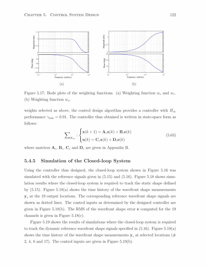
Chapter 5. Control System Design 122
0
0.5
1
1.5M
agni
tude
(ab
s)
10−1
100
101
102
−180
−135
−90
−45
0
Pha
se (
deg)
Frequency (rad/sec)
(a)
0
0.5
1
Mag
nitu
de (
abs)
10−1
100
101
102
0
30
60
90
Pha
se (
deg)
Frequency (rad/sec)
(b)
Figure 5.17: Bode plots of the weighting functions. (a) Weighting function we and wr.
(b) Weighting function wu.
weights selected as above, the control design algorithm provides a controller with H∞
performance γmin = 0.91. The controller thus obtained is written in state-space form as
follows:
∑
K∞
:
x(k + 1) = Acx(k) + Bce(k)
u(k) = Ccx(k) + Dce(k)(5.63)
where matrices Ac, Bc, Cc and Dc are given in Appendix B.
5.4.5 Simulation of the Closed-loop System
Using the controller thus designed, the closed-loop system shown in Figure 5.16 was
simulated with the reference signals given in (5.15) and (5.16). Figure 5.18 shows simu-
lation results where the closed-loop system is required to track the static shape defined
by (5.15). Figure 5.18(a) shows the time history of the wavefront shape measurements
ys at the 19 output locations. The corresponding reference wavefront shape signals are
shown as dotted lines. The control inputs as determined by the designed controller are
given in Figure 5.18(b). The RMS of the wavefront shape error e computed for the 19
channels is given in Figure 5.18(c).
Figure 5.19 shows the results of simulations where the closed-loop system is required
to track the dynamic reference wavefront shape signals specified in (5.16). Figure 5.19(a)
shows the time history of the wavefront shape measurements ys at selected locations (#
2, 4, 8 and 17). The control inputs are given in Figure 5.19(b).
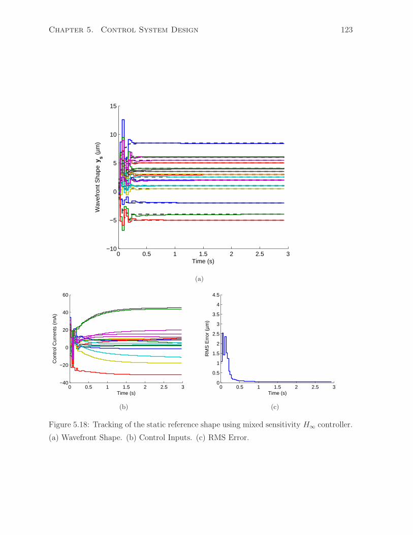
Chapter 5. Control System Design 123
0 0.5 1 1.5 2 2.5 3−10
−5
0
5
10
15
Time (s)
Wav
efro
nt S
hape
ys (
µm)
(a)
0 0.5 1 1.5 2 2.5 3−40
−20
0
20
40
60
Time (s)
Con
trol
Cur
rent
s (m
A)
(b)
0 0.5 1 1.5 2 2.5 30
0.5
1
1.5
2
2.5
3
3.5
4
4.5
Time (s)
RM
S E
rror
(µm
)
(c)
Figure 5.18: Tracking of the static reference shape using mixed sensitivity H∞ controller.
(a) Wavefront Shape. (b) Control Inputs. (c) RMS Error.

Chapter 5. Control System Design 124
0 0.5 1 1.5 2 2.5 3−6
−4
−2
0
2
4
6
8
10
Time (s)
Wav
efro
nt S
hape
ys (
µm)
(a)
0 0.5 1 1.5 2 2.5 3−40
−30
−20
−10
0
10
20
30
40
Time (s)
Con
trol
Cur
rent
s (m
A)
(b)
0 0.5 1 1.5 2 2.5 30
0.5
1
1.5
2
2.5
3
3.5
4
4.5
Time (s)
RM
S E
rror
(µm
)
(c)
Figure 5.19: Tracking of the dynamic reference shape using mixed sensitivity H∞ con-
troller. (a) Wavefront Shape. (b) Control Inputs. (c) RMS Error.

Chapter 5. Control System Design 125
As is evident from Figure 5.18 and 5.19, the H∞ controller tracks both the static
and the dynamic wavefront shape signals with adequate performance. Note that the
measured wavefront shape ys follows the sinusoidal reference signals perfectly as can be
seen in Figure 5.19(a).
5.5 Summary
In this chapter, three different control algorithms have been presented. Firstly, con-
sidering the MFDM as a static system, a PI controller was designed based on a DC-
decoupled static plant model. The simulations performed using this controller showed
that this type of controllers can be successfully applied to the MFDMs designed according
to the modification proposed in this thesis. Secondly, a decentralized robust PID con-
troller is presented where the uncertainties in the modeling of the DC-decoupled plant
model are accounted for in the controller design process. The resulting closed-loop system
successfully achieved tracking of static reference wavefront shapes. However, when track-
ing reference signals having relatively high frequency components, a significant phase
lag between the reference signals and the measured wavefront ys is observed. Finally, a
controller with H∞ optimal performance was designed using the mixed-sensitivity H∞
technique. Simulation results of the resulting closed loop system show that effective
tracking of both the static and the dynamic signals in the desired range of frequencies
can be achieved.

Chapter 6
Experimental Results and Discussion
This chapter is aimed at experimentally validating the analytical model developed in
chapter 3 and evaluating the performance of the control algorithms developed in chapter
5 using the prototype MFDM and the AO setup described in chapter 4.
After some preliminaries given in the following section, the analytical model is vali-
dated by comparing the predictions made by the model with the corresponding experi-
mental results. The effects of the linearization of the MFDM response using a Helmholtz
coil are investigated and verified in section 6.3. The experimental evaluation of the per-
formance of the controllers presented in chapter 5 is given in section 6.4. A summary of
the results is given in section 6.6.
6.1 Preliminaries
6.1.1 Parameter Settings
Before presenting the experimental results, it is pertinent to specify the settings used in
obtaining the results. The common settings are listed as follows:
• The magnetic fluid properties used in the analytical model of the MFDM are those
of EFH1 as listed in Table 3.1.
• The MFDM model (3.90) is truncated to the following numbers of radial and az-
imuthal modes, respectively: N = 4, M = 4. The resulting state space model is
given in Appendix B.
126

Chapter 6. Experimental Results and Discussion 127
• All results are obtained using a magnetic fluid layer which has a thickness of 1.0
mm.
• If not otherwise stated, the Helmholtz coil is set to run at 194 mA current, which
corresponds to a nominal magnetic flux density of 2.5 mT.
• The optical pupil size i.e., the diameter of the laser beam, is set to 22 mm as
measured on the MFDM surface. All optical metrics, e.g. the PSF and the RMS
of the wavefront shape error, are computed using this pupil size.
6.1.2 System Identification
System identification (SI) is a black-box approach to system modeling, which is used to
estimate models of dynamic systems from experimentally measured input-output data.
A supplementary model of the dynamics of the MFDM surface shape was obtained using
this approach and has been used in the validation of the analytical model. The identified
model of the dynamics of the MFDM surface shape is briefly described here.
The identified model is obtained using the System Identification Toolbox of Matlab R©
[115]. Multiple sets of input-output data are generated by applying suitable currents
to the electromagnetic coils and measuring the surface deflections at selected output
positions using the wavefront sensor. The input-output data is then fit to a pre-specified
model structure. The prediction-error minimization method [116] is used to estimate a
discrete-time state-space model ΣSysID of the MFDM response:
ΣSysID :
x(k + 1) = Ax(k) + Bu(k)
y(k) = Cx(k) + Du(k)(6.1)
where u and y are the experimentally generated inputs and outputs, respectively, and
A, B, C, D are the estimated system matrices.
To get the best estimates of the system matrices, multiple sets of input-output data
are generated by applying step, sinusoidal and multi-frequency inputs to each of the input
channels and observing the outputs over time. The data is pre-processed by removing
any spurious readings and trends. One set of data, obtained with the multi-frequency
inputs, is used as the primary data for identification, while the remaining sets are used for
validation purpose. The identification process is done iteratively such that the prediction

Chapter 6. Experimental Results and Discussion 128
error is minimized while the estimates of the system matrices are updated in each iter-
ation. The order of the system is gradually increased until the simulated model output
best fits the measured data. The identified model thus obtained is given in Appendix B.
6.1.3 Jones’ Model of Static Response
In the validation of the analytical model that will follow, in addition to comparing the
predictions of the analytical model with the experimental results, a static model of the
mirror response will also be used for comparison. The static model has been adapted from
an existing model of the displacements of the free surface of a magnetic fluid presented
by Jones [104]. Using Jones’ model, the displacements of the free surface of a magnetic
fluid produced by an applied magnetic field with the flux density bz can be written as:
ζ =χb2z2ρgµ
(6.2)
As presented here, the model is applicable to the special case where the magnetic fluid
surface is exposed to a vertical magnetic field i.e., the flux density of the magnetic field
has only a vertical component bz and no horizontal component. Jones’ model can be
utilized to derive the displacement of the MFDM surface where a large magnetic field
with the flux density B0 is superimposed on a smaller magnetic field with the flux density
bz and where both of the fields are acting in the vertical direction. The derived surface
displacements in this case can be found as:
ζ =χbzB0
ρgµ(6.3)
This model can be used to obtain static displacements of the MFDM surface at the
surface locations where the magnetic field of the miniature electromagnetic coils presents
only a vertical component and no horizontal component. One such location is the peak
of the surface shape produced by applying current input to only one electromagnetic coil
and will be used in the following paragraphs for the comparison of the analytical model
with Jone’s model.
6.1.4 Initial Surface Map and Measurement Noise
The experimental results presented in this chapter are based on wavefront shape measure-
ments obtained using a Shack-Hartmann wavefront sensor. Before presenting the results,
a brief discussion on the accuracy of the measurements is presented in this section.

Chapter 6. Experimental Results and Discussion 129
Theoretically, in absence of any input currents applied to the wavefront corrector and
with no externally induced wavefront aberrations, the wavefront shape as measured by
the wavefront sensor should be a perfect planar surface. However, practically achiev-
ing this is almost impossible because the optical and electromechanical components of
system itself induce aberrations, which cannot be completely eliminated in the initial
process of installation and alignment of these components. Therefore, the wavefront
sensor reads an initial wavefront shape ys0 that needs to be taken into consideration in
all subsequent measurements. The initial wavefront shape is dynamic in nature i.e., it
varies over time. However, the initial wavefront shape measurement ys0 has a relative
large mean component that can be considered to be static and is called the initial surface
map. It is a common practice in AO systems that the effect of the initial surface map
is canceled out by giving a bias to the wavefront corrector using a set of initial inputs.
On the other hand, the dynamic component of the initial wavefront shape measurement
remains uncorrected. The static and the dynamic components of the initial wavefront
shape measurement are discussed in the following.
Static Surface Map
The initial static surface map and the set of inputs used to cancel its effect were deter-
mined as follows. With no inputs applied to the MFDM, a series of wavefront measure-
ments is taken such that at any instant k, k = 1, 2, ..., K, ys0(k) is a vector of wavefront
shape displacements measured at M discrete lenslet locations contained in the optical
pupil. The initial static surface map is obtained as a mean surface defined by
ys0 =1
K
K∑
k=1
ys0(k) (6.4)
Once the initial static surface map ys0 is known, the vector of input currents needed to
cancel its effect can be obtained as follows:
u0 = G−10 ys0 (6.5)
where G0 is the DC gain of the system as given in (5.8). The application of this initial
bias flattens the resulting wavefront shape, which becomes the reference for all subsequent
wavefront shape measurements. Before applying any input currents computed in order to
produce any desired wavefront shape, the initial input currents are added to these inputs.
The surface plot of the initial surface map of the setup used to obtain the results presented

Chapter 6. Experimental Results and Discussion 130
x (mm)
y (m
m)
RMS = 0.497µm
−10 −5 0 5 10
−10
−5
0
5
10
−0.6
−0.5
−0.4
−0.3
−0.2
−0.1
0
0.1
Figure 6.1: Initial surface map.
x (mm)
y (m
m)
RMS = 0.171µm
−10 −5 0 5 10
−10
−5
0
5
10
Figure 6.2: Flattened surface.
in this chapter is given in Figure 6.1. The set of input currents needed to flatten the sur-
face is given as: u0 = [−0.4, 3.7, 23.6, 14.5, 28.0, 9.8, 17.3, 14.0, −9.9, 12.8, 11.4, 7.5, ...
8.4, −2.9, 3.1, 2.2, −15.9, 19.8, 7.3]T × 131.5×103 A. The surface plot of the resulting wave-
front shape obtained after applying the bias currents is given in Figure 6.2.
Dynamic Noise Component
The dynamic component of the initial wavefront shape remains uncorrected in the open-
loop measurements and can be considered as measurement noise. Unless mitigated by
closed-loop control system, the measurement noise poses a limit on the performance of
the AO system. An estimate of the magnitude of the measurement noise can be obtained
by computing the standard deviation of the initial wavefront shape measurements ys0(k)

Chapter 6. Experimental Results and Discussion 131
give as
σ =
√√√√ 1
K
K∑
k=1
(ys0(k) − ys0)2 (6.6)
The mean of the standard deviations computed over the 19 surface locations corre-
sponding to the 19 actuator coils was found to be 0.181 µm. Another similar measure
of the dynamic component of the initial surface shape is the standard deviation of the
RMS values computed at instants k, k = 1, 2, ..., K. The computed standard deviation
of the RMS values of the experimentally obtained initial surface shapes is 0.173 µm.
6.2 Model Validation
The results of an experimental investigation aimed at validating the analytical model are
presented in this section. In the following sub-section, the static response of the prototype
MFDM is compared to the response predicted by the analytical model. The dynamic
characteristics of the mirror as predicted by the model are experimentally validated in
section 6.2.2.
6.2.1 Static Response
As the first step toward validating the analytical model, the static surface deflections
predicted by the model are compared with those obtained experimentally. The steady-
state response of the MFDM surface can be analytically derived from the state-space
model given in (3.90) and is given as:
yss = −CA−1Buss (6.7)
where uss is the vector of constant currents applied to the array of 19 electromagnetic
coils and the system matrices A, B and C are given in Appendix B. The steady-state
response of the surface to a set of constant input currents is a static surface shape, which
can be obtained from (6.7). The static response of the actual MFDM can be directly
measured using the wavefront sensor.
Figure 6.3 presents the comparison of the experimentally obtained surface deflections
with those predicted by the presented model. The figure shows the surface deflections
resulting from applying various input currents to only the center coil (coil# 1 in Figure
4.6). Since the resulting deflections are symmetric about the vertical axis, only 2D

Chapter 6. Experimental Results and Discussion 132
−10 −5 0 5 10
−10
−5
0
5
10
Radial Distance r (mm)
Sur
face
Def
lect
ion
ζ (µ
m)
ExperimentalAnalytical
38.0 mA
31.7 mA
25.4 mA
19.0 mA
12.7 mA
6.3 mA
−6.3 mA
−12.7 mA
−19.0 mA
−25.4 mA
−31.7 mA
−38.1 mA
Figure 6.3: Comparison of the static surface shapes obtained experimentally vs. those
predicted analytically.
surface shapes are shown. The RMS of the error between the two corresponding surfaces
computed over the 22 mm pupil is shown in Figure 6.4. It is evident from the computed
RMS errors that the steady-state surface deflections predicted by the presented model
closely agree with those obtained experimentally. Besides the comparable deflections,
the model also reveals the Gaussian profile of the deformed surface.
The peak surface displacement predicted by the analytical model can also be compared
to those given by Jones’ model as given in (6.3). Figure 6.5 shows the comparison,
where it can be observed that the analytical model shows a better conformance to the
experimental results than Jones’ model. It is reiterated that the comparison of the Jones’
model to both the experimental results and the analytical model presented in this thesis is
valid only for the peak surface displacements where the magnetic field has only a vertical
component and the horizontal component is zero. It may also be noted that, contrary
to the analytical model presented in this thesis, Jones’ model does not consider surface
tension of the magnetic fluid.
The analytical model (3.90) represents a MIMO system. Experiments show that
the surface deflections determined by the model are just as valid for the simultaneously
applied multiple inputs as for the case of the single input. The 3D surface shapes resulting
from a specified set of input currents u = [0.1, 0.5, 0.4, 0.3, 0.1, −0.1, 0.2, 0.9, 0.7, ...

Chapter 6. Experimental Results and Discussion 133
−50 −40 −30 −20 −10 0 10 20 30 40 500
0.05
0.1
0.15
0.2
0.25
0.3
0.35
Current (mA)
RM
S E
rror
(µm
)
Figure 6.4: RMS error between the analytical and experimental surface shapes of the
MFDM measured at different input currents.
−40 −30 −20 −10 0 10 20 30 40−15
−10
−5
0
5
10
15
Current (mA)
Sur
face
Def
lect
ion
ζ (µ
m)
ExperimentalAnalytical − with STAnalytical − without STJones Model
Figure 6.5: Comparison of the peak surface displacements given by the analytical model,
Jones’ model [104] and the experimental results.

Chapter 6. Experimental Results and Discussion 134
−10
0
10
−10
−5
0
5
10
−10
−5
0
5
10
x (mm)y (mm)
ζ (µ
m)
(a)
−10
0
10
−10
−5
0
5
10−10
−5
0
5
10
x (mm)y (mm)
ζ (µ
m)
(b)
x (mm)
y (m
m)
0.640.31
−0.0
17−0
.35
−0.68
−1−1
.3
−0.017
−0.017
−10 −5 0 5 10
−10
−5
0
5
10
−20
−15
−10
−5
0
5
10
15
20
(c)
Figure 6.6: Comparison of the 3D static surface shapes. (a) Analytical. (b) Experimental.
(c) Error. (The color bar and contour labels show the surface shapes in micrometers.)
0.6, −0.5, 0.6, 0.1,−0.4, −0.9, −0.3, 0.5, −0.3, 0.4]T × 131.5
A applied to the array of 19
coils, are presented for comparison of the analytically predicted surface shapes with
those obtained experimentally. Figure 6.6(a) shows the surface shape predicted by the
analytical model. The corresponding shape obtained by applying the currents to the
prototype MFDM is given in Figure 6.6(b). Figure 6.6(c) shows the contour plot of the
shape error computed as the difference of the surfaces shapes shown in 6.6(a) and 6.6(b).
The contours are spaced at λ2, where λ is the wavelength of the laser light used. The RMS
of the shape error computed using the discrete displacements at the wavefront sensor
lenslet locations contained in the pupil, is 0.19µm. Given the noise conditions in the
laboratory as discussed in section 6.1.4, the resulting RMS error shows that the surface
shape predicted by the analytical model compares fairly well with the experimentally
obtained shape.

Chapter 6. Experimental Results and Discussion 135
6.2.2 Dynamic Response
In the following, important dynamic response parameters predicted by the model are
compared with the corresponding experimental results. The dynamic response of the
MFDM surface to a step, a sinusoidal and a multitone input is presented. The bode plots
of the analytical model and the identified model are compared and important features
highlighted by the plots are discussed.
Response to a Step Input
Figure 6.7 presents a comparison between the step response of the actual MFDM and that
of the analytical model of the mirror. A step input of 1 volt is applied to the center coil
(coil# 1 in Figure 4.6) of the MFDM. The time history of the mirror surface deflections
immediately above the center of the coil is noted and plotted as shown in Figure 6.7(a).
The response of the actual mirror surface is shown by the solid line (blue) while the
analytically determined surface deflections are represented by the dashed line (red). The
deflections predicted by the identified model are given as the dash-dotted line (magenta).
For a direct visual comparison, the input current applied to the electromagnetic coil is
scaled appropriately and is plotted against the right hand side axis. The input current
plot is shown as the dotted line (black). The error in the analytically predicted surface
displacements as measured against the experimental results and the predictions of the
identified model is presented in Figure 6.7(b). As can be observed from the figure, the
response given by the analytical model agrees fairly well with the experimental results
as well as with the identified model.
Response to a Sinusoidal Input
Figure 6.8 shows the response of the MFDM to a sinusoidal signal with 3 Hz frequency
and an amplitude of 1 volt. Again, the input signal is applied to the center coil (coil#
1 in Figure 4.6). The output is measured at the location immediately above the center
of the coil and is plotted in Figure 6.8(a). The experimentally obtained deflections of
the mirror surface are represented by the solid line (blue); the response obtained using
the analytical model is shown by the dashed line (red); the dash-dotted line (magenta)
represents the response given by the identified model. The sinusoidal input current is
shown on the right hand side axis with the plot drawn using a dotted line (black). Note
that the scale of the right hand side axis is the same as the one used in the response to

Chapter 6. Experimental Results and Discussion 136
the step input plotted in Figure 6.7 above thus highlighting the drop in the amplitude of
the output surface deflections with the increased frequency of the input current signal.
The error in the analytically predicted surface displacements as measured against the
experimental results and the predictions of the identified model is presented in Figure
6.8(b). Although a significant error can be seen in the shown plot, it remains less than
10% of the peak-to-valley deflections of 15 µm as shown in Figure 6.8(a).
Response to a Multitone Input
Figure 6.9 shows the response of the MFDM surface to a multitone signal where the
input current frequency varies over time. The input signal is given by:
u1 = I0 sin
(
2π
(
f1 +f2 − f1
Tt
)
t
)
(6.8)
where I0 = 31.75 mA is the amplitude of the input current signal and the frequency of
the signal linearly varies from f1 = 0 to f2 = 5 Hz in T = 5 seconds. Figure 6.9(a) shows
a comparison of the analytically predicted surface deflection against the experimental
results and surface displacements predicted by the identified model. The corresponding
error is shown in Figure 6.9(b). It is evident from the comparison of the response given
by the analytical model to the experimental results as well as to the response given by
the identified model that there exists good agreement among all three results. With the
increasing frequency of the input current signal, certain trends in the experimental results
can be observed. It can be seen that the output surface displacements follow the driving
input closely in the low frequency range. The agreement deteriorates as the frequency is
increased. Firstly, the amplitude of the surface deflections decreases with the increasing
frequency. Secondly, there exists a phase lag between the input current signal and the
output displacements, which increases with the increasing frequency. It is evident from
the presented plots that analytical model captures both these trends and closely follows
the experimental results. On both trends, the analytical model agrees with the identified
model as well.
Bode Plots
Bode plots present a comprehensive picture of the dynamics of a system. Figure 6.10
shows the Bode plots of the analytical model and the identified model of the plant. The
plots presented are for the system where the input current is applied at the center coil
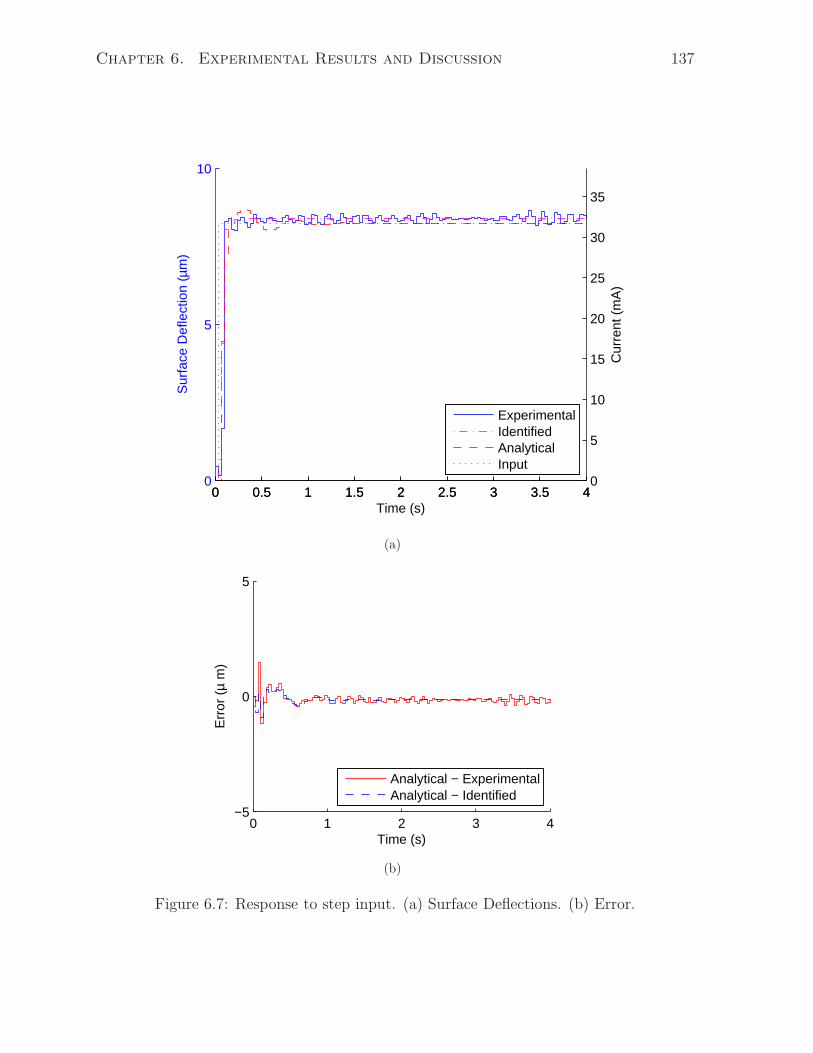
Chapter 6. Experimental Results and Discussion 137
0 0.5 1 1.5 2 2.5 3 3.5 40
5
10S
urfa
ce D
efle
ctio
n (µ
m)
Time (s)
0 0.5 1 1.5 2 2.5 3 3.5 40
5
10
15
20
25
30
35
Cur
rent
(m
A)
ExperimentalIdentifiedAnalyticalInput
(a)
0 1 2 3 4−5
0
5
Time (s)
Err
or (
µ m
)
Analytical − ExperimentalAnalytical − Identified
(b)
Figure 6.7: Response to step input. (a) Surface Deflections. (b) Error.
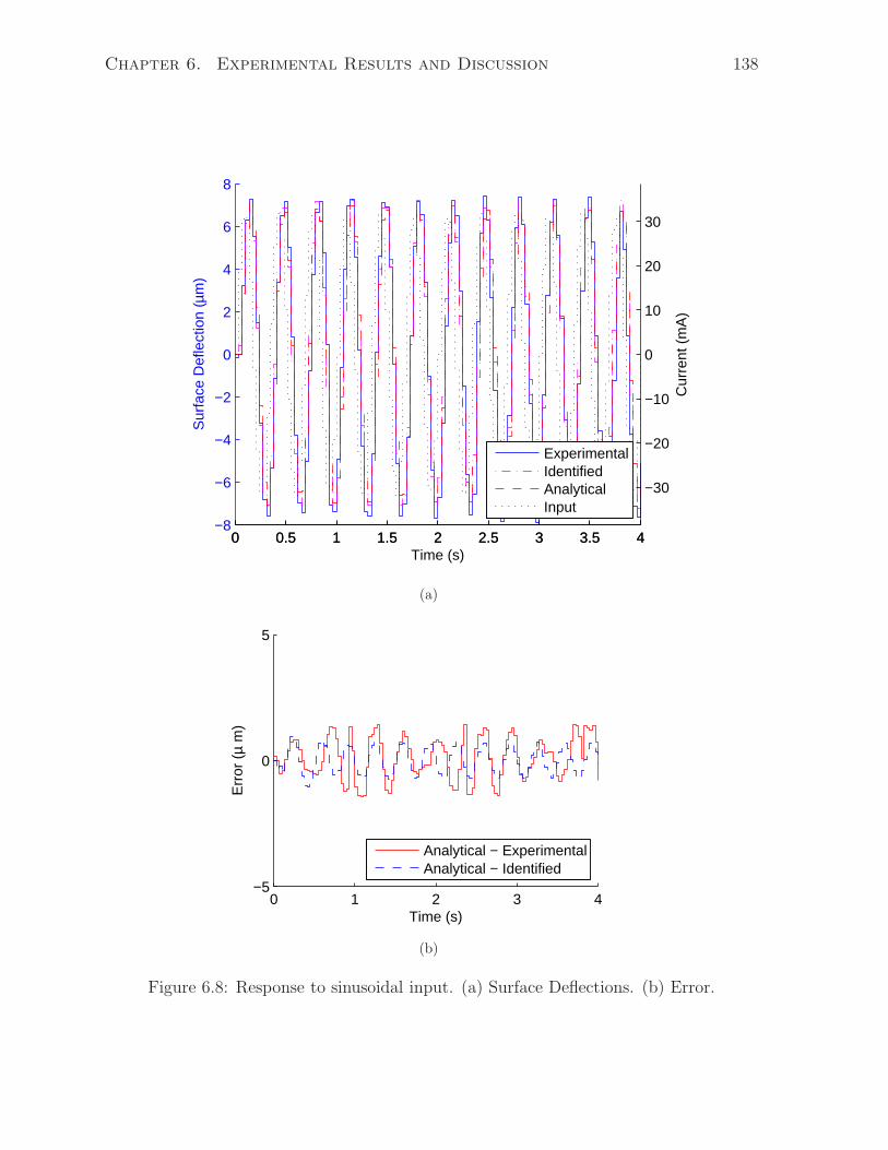
Chapter 6. Experimental Results and Discussion 138
0 0.5 1 1.5 2 2.5 3 3.5 4−8
−6
−4
−2
0
2
4
6
8S
urfa
ce D
efle
ctio
n (µ
m)
Time (s)
0 0.5 1 1.5 2 2.5 3 3.5 4
−30
−20
−10
0
10
20
30
Cur
rent
(m
A)
ExperimentalIdentifiedAnalyticalInput
(a)
0 1 2 3 4−5
0
5
Time (s)
Err
or (
µ m
)
Analytical − ExperimentalAnalytical − Identified
(b)
Figure 6.8: Response to sinusoidal input. (a) Surface Deflections. (b) Error.
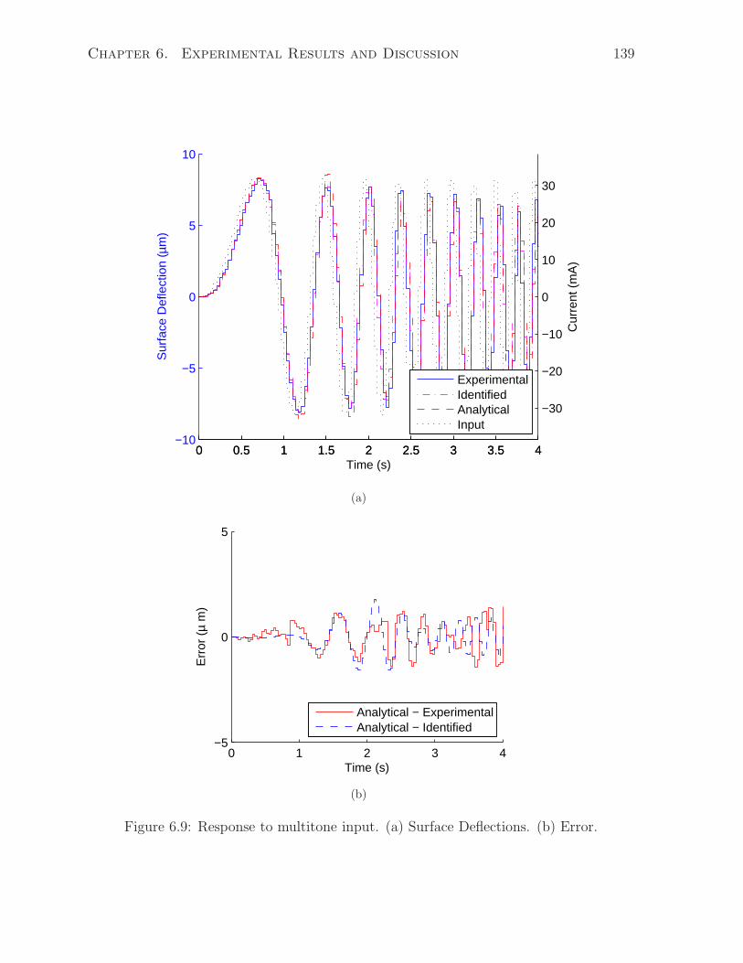
Chapter 6. Experimental Results and Discussion 139
0 0.5 1 1.5 2 2.5 3 3.5 4−10
−5
0
5
10S
urfa
ce D
efle
ctio
n (µ
m)
Time (s)
0 0.5 1 1.5 2 2.5 3 3.5 4
−30
−20
−10
0
10
20
30
Cur
rent
(m
A)
ExperimentalIdentifiedAnalyticalInput
(a)
0 1 2 3 4−5
0
5
Time (s)
Err
or (
µ m
)
Analytical − ExperimentalAnalytical − Identified
(b)
Figure 6.9: Response to multitone input. (a) Surface Deflections. (b) Error.

Chapter 6. Experimental Results and Discussion 140
0
5
10
15
20
Mag
nitu
de (
abs)
10−1
100
101
102
−450
−360
−270
−180
−90
0
Pha
se (
deg)
Frequency (rad/sec)
AnalyticalIdentified
Figure 6.10: Bode plot of the SISO system.
(coil 1 in Figure 4.6) of the MFDM and the output wavefront displacement is measured
at the location of the corresponding input coil. The analytical model agrees well with
the identified model in the low frequency range. Some mismatch between the two models
appears for frequencies beyond 10 rad/sec. Some important characteristics of the mirror
response can also be observed from the Bode plots. The MDFM features a bandwidth 1
of approximately 20 rad/sec. Secondly, there exists a significant phase lag in the response
of the mirror surface, which increases with the increasing frequency. This explains the
lag between the input currents and the output surface deflections as plotted in Figure
6.9 above.
The results presented above for the validation of the analytical model show that there
exists a very close agreement between the response of the MFDM system as predicted by
the analytical model and the corresponding results obtained experimentally. Similarly,
these two results also agree fairly well with the response of the system as predicted by
the identified model.
1The first frequency where the gain drops below 70.79 percent (-3 dB) of its DC value.

Chapter 6. Experimental Results and Discussion 141
−40 −30 −20 −10 0 10 20 30 40−15
−10
−5
0
5
10
15
Current (mA)
Sur
face
Def
lect
ion
ζ (µ
m)
ExperimentalAnalytical − with STAnalytical − without STJones Model
Figure 6.11: Effect of surface tension on the peak surface displacements.
6.2.3 Effects of Surface Tension
The effects of surface tension in the magnetic fluid become evident when comparing the
experimentally obtained peak displacements with those predicted by the analytical model,
with and without including the surface tension. Such a comparison is made in Figure
6.11 where the peak surface deflections already presented in Figure 6.5 are reproduced
with the predictions of the analytical model presented for both the cases i.e., with and
without considering surface tension (ST). It is obvious from the figure that the surface
tension plays a significant role in determining the response of the mirror. It may be noted
that the predictions of the analytical model and those provided by Jones’ model (6.3)
coincide when the effects of surface tension are not included in the analytical model.
6.3 Linearity of the MFDM Response
A significant contribution of the work presented in this thesis is the linearization of the
response of the MFDM, which is achieved by incorporating a Helmholtz coil in the design
of the mirror. Experimental results which validate the proposed design modification and
its effect on the response of the MFDM surface are presented here. First, the response of a
MFDM, which uses the miniature coils only, is demonstrated by disabling the Helmholtz
coil of the prototype mirror and recording the surface displacements as a function of the

Chapter 6. Experimental Results and Discussion 142
current applied to one of the miniature coils. Then, the linearizing effect of the Helmholtz
coil is captured by observing the surface displacements while the Helmholtz coil is turned
on. Finally, the proposition is substantiated by testing the principle of superposition of
the response of the fluid surface.
Figure 6.12 shows the peak surface deflections as a function of currents applied to
the miniature coil in the center of the mirror. The points marked as ′∗′ signify the peak
surface deflections of the MFDM when the Helmholtz coil is disabled. It can be seen
that the surface deflections are positive for both positive and negative polarities of the
input current applied to the miniature coil. Also, the surface deflections are non-linear
with respect to the applied current. A trend line fitted on the data reveals a quadratic
approximation. This behavior can be explained using Jones’ model of the static response
of the fluid surface as given in (6.2). The model shows that the displacement ζ of a
magnetic fluid surface exposed to a magnetic field is a quadratic function of the magnetic
flux bz of the field. The magnetic flux, in turn, is a linear function of the applied current
implying that the surface deflection ζ is a quadratic function of the applied current.
The experimental peak surface deflections for the case when the Helmholtz coil is
turn on are marked as ′′. It is obvious that (1) the surface deflections vary linearly with
the increasing currents applied to the coil, and (2) both negative and positive deflections
are achieved.
The experimental results also show that when the Helmholtz coil is turned on, the
principle of superposition holds distinctly. As illustrated in Figure 6.13, when the two
coils marked 1 and 2 (see Figure 4.6) are energized, the surface deflection (′∆′) at a point
midway between the two coils is the sum of the deflections (′+′ and ′′) at this point
generated by each of the two coils energized separately. It is therefore evident that the
proposed change in the design of the MFDM does produce the desired effect of linearizing
the response of the mirror surface.
6.3.1 Bi-directional Displacements
The linearity of the response of the mirror also allows bidirectional displacements. Under
the conventional design, the magnetic fluid can ’push’ only but not ’pull’ [15]. Due to
this limitation of conventional MFDMs, the pulling effect is generated by biasing the
electromagnetic coils to 50% of their maximum ’push’, which results in a reduction of
the maximum achievable deflection by half. The design proposed in this thesis resolves

Chapter 6. Experimental Results and Discussion 143
−40 −30 −20 −10 0 10 20 30 40
−10
−5
0
5
10
Current (mA)
Sur
face
Def
lect
ion
ζ (µ
m)
Helmholtz coil inactiveHelmholtz coil active
Figure 6.12: Comparison of the response of the MFDM with conventional design vs.
proposed design.
−40 −30 −20 −10 0 10 20 30 40
−10
−5
0
5
10
Current (mA)
Sur
face
Def
lect
ion
ζ (µ
m)
Coil 1 activeCoil 2 activeBoth coils active
Figure 6.13: Illustration of the principle of superposition of the MFDM surface displace-
ments.

Chapter 6. Experimental Results and Discussion 144
−200 −150 −100 −50 0 50 100 150 200−10
−8
−6
−4
−2
0
2
4
6
8
10
Current − Helmholtz Coil (mA)
Sur
face
Def
lect
ion
ζ (µ
m)
Figure 6.14: Illustration of the amplifying effect of the large, uniform magnetic field
generated using the Helmholtz coil. The plot shows the peak surface deflections as a
function of the current applied to the Helmholtz coil while the current applied to the
miniature coil is kept constant at 1 V.
this problem by generating both positive and negative displacements.
6.3.2 Amplification of the Surface Deflections
Another significant aspect of the proposed design modification is the amplification of the
surface deflections achieved by applying the large uniform magnetic field. The amplifica-
tion effect of this field provided by the Helmholtz coil can be seen in Figure 6.14 where
the current applied to the Helmholtz coil is gradually increased while the current applied
to the miniature coil (#1 in Figure 4.6) is kept constant at 1 volt. Note that the polarity
of the current applied to the Helmholtz coil also has the effect of reversing the ’push’ or
’pull’ to the mirror surface.
It may be noted that the magnetic field of the miniature coils generates the desired
shape of the mirror surface. The large uniform magnetic field, on the other hand, amplifies
the magnitude of the surface displacements. A very significant connotation of this effect
is that very small electromagnetic coils can be used in conjunction with an appropriately
large uniform magnetic field to produce far larger surface deflections than those possible
with the small coils only. This will allow fabrication of very small mirrors - most likely

Chapter 6. Experimental Results and Discussion 145
0 0.5 1 1.5 2 2.5 3−6
−4
−2
0
2
4
6
8
10
Time (s)
Wav
efro
nt S
hape
ys (
µm)
(a)
0 0.5 1 1.5 2 2.5 30
0.5
1
1.5
2
2.5
3
3.5
4
4.5
Time (s)
RM
S E
rror
(µm
)
SimulatedExperimental
(b)
Figure 6.15: Experimental tracking of a static reference shape using the PI controller.
(a) Wavefront Shape. (b) RMS Error.
developed using one of the MEMS microfabrication methods - with sufficient actuator
density and surface deflections for possibly all applications of MFDMs.
6.4 Controller Performance Evaluation
This section presents the results of the experimental work carried out to evaluate the
performance of the controllers presented in chapter 5. Where possible, a comparison to
the numerical simulations given in chapter 5 is also presented.
6.4.1 Decentralized PI Controller with DC Decoupling
In order to implement the decentralized PI controller as presented in section 5.2, the
closed-loop system shown in Figure 5.4 is constructed such that the augmented plant G
is the actual system comprising the MFDM and the sensor. The controller K = kG−10
where the parameters in k are provided by (5.14) and G−10 is obtained from (5.8).
With the closed-loop system thus setup, the static reference wavefront shape signals
specified in (5.15) are tracked by the system. Figure 6.15(a) shows the time history of
the experimentally obtained wavefront shape measurements ys. For clarity only selected
channels (# 2, 4, 8 and 17) are displayed. The corresponding reference signals are shown
as dotted lines (black). The RMS of the wavefront shape error e is given in Figure 6.15(b)
where the corresponding simulation results are also shown for comparison. While the

Chapter 6. Experimental Results and Discussion 146
simulations showed that the controller can drive the RMS error to zero, the experimental
results show a residual steady-state error of 0.26 ± 0.05µm. The error is within the
acceptable limits since the measured noise level is of the same order as the observed
RMS error.
The experiments conducted with the dynamic reference wavefront shape signals (5.16)
show that the PI controller can track very slowly changing signals only. With the in-
creasing frequency of the reference signals, the error increases rapidly and results in the
saturation of the actuator electromagnetic coils.
6.4.2 Decentralized Robust PID Controller
The decentralized robust PID controller is implemented by setting up a closed-loop sys-
tem as was shown in Figure 5.4, where the plant G is the actual system comprising
the MFDM and the sensor. The controller given in (5.57) is used with the same PID
parameters as given in (5.54). The error signal e is filtered using the discretized version
of the low pass filter W(s) (5.52).
The ability of the closed-loop system to compensate for the high-order, static aber-
rations is tested by tracking the reference wavefront shape signals as given in (5.15).
Figure 6.16 shows the time history of the wavefront shape measurements ys at selected
channels (# 2, 4, 8 and 17). RMS of the wavefront shape error e in tracking of the
reference wavefront shape signals is given in Figure 6.16(b). The RMS error of the sim-
ulated closed-loop system is also plotted for comparison. The experimental results show
a steady-state RMS error of 0.24 ± 0.05µm.
The ability of the controller to track dynamic surface shapes was tested using the
reference wavefront shape signals specified in (5.16) where fo = 3Hz. Figure 6.17(a)
shows the time history of the experimentally obtained wavefront shape measurements ys.
The RMS of the wavefront shape error is shown in Figure 6.17(b). As can be observed
from the figure, the controller does manage to track the specified reference wavefront
shape, however, a significant error remains uncorrected.
6.4.3 Mixed Sensitivity H∞ Controller
The H∞ controller is implemented by incorporating the controller (5.58) into the closed-
loop system as shown in Figure 5.16 with the weighting functions omitted. The state-
space representation of the controller is provided in Appendix B. The augmented plant

Chapter 6. Experimental Results and Discussion 147
0 0.5 1 1.5 2 2.5 3−6
−4
−2
0
2
4
6
8
10
Time (s)
Wav
efro
nt S
hape
ys (
µm)
(a)
0 0.5 1 1.5 2 2.5 30
0.5
1
1.5
2
2.5
3
3.5
4
4.5
Time (s)
RM
S E
rror
(µm
)
SimulatedExperimental
(b)
Figure 6.16: Experimental tracking of a static reference shape using the robust PID
controller. (a) Wavefront Shape. (b) RMS Error.
0 0.5 1 1.5 2 2.5 3−6
−4
−2
0
2
4
6
8
10
Time (s)
Wav
efro
nt S
hape
ys (
µm)
(a)
0 0.5 1 1.5 2 2.5 30
0.5
1
1.5
2
2.5
3
3.5
4
4.5
Time (s)
RM
S E
rror
(µm
)
SimulatedExperimental
(b)
Figure 6.17: Experimental tracking of a dynamic reference shape using the robust PID
controller. (a) Wavefront Shape. (b) RMS Error.

Chapter 6. Experimental Results and Discussion 148
G represents the actual system comprising the mirror and the sensor.
For the static reference wavefront shape signals as given in (5.15), the controller
performance can be seen in Figure 6.18(a) where only selected channels (# 2, 4, 8 and
17) are shown. As can be seen in the figure, the controller tracks the static reference
signals fairly well, and rapidly drives the mirror surface deflections to their steady states.
RMS of the wavefront shape error is shown in Figure 6.18(b) and has a steady-state
value of 0.35 ± 0.05µm. Again for comparison, the RMS error of the simulated closed-
loop system is plotted alongside experimental results.
The experimental results for tracking of the dynamic reference wavefront shape signals
are given in Figure 6.19. The wavefront shape measurements ys are plotted in Figure
6.19(a) where the corresponding reference wavefront shape signals are shown by dotted
lines (black). The RMS of the wavefront shape error computed over the 19 output points
is plotted in Figure 6.19(b). Although there remains a significant ripple in the RMS
error, clearly the H∞ controller can be seen to be tracking the sinusoids much better
than the robust PID controller.
6.4.4 Comparison of the Controllers
A quick comparison of the three controllers is presented in Figure 6.20 where the RMS
errors in tracking of the static and dynamic reference wavefront shape signals using these
controllers are plotted together. It is obvious that the all three controllers perform fairly
well in tracking static wavefront shape signals. As for the dynamic shapes, the PI con-
troller was found to be lacking the ability of tracking the specified reference signals over
the desired range of frequencies. The robust PID controller performed adequately well
over the desired range of frequencies. However, a significant error remains uncorrected.
The H∞ controller satisfactorily tracks sinusoidal signals with frequencies up to 3 Hz.
6.5 Performance Evaluation
In this section, the performance limits of the MFDM in canceling high-order wavefront
aberrations are tested. In the following subsection, the spatial resolution of the wave-
front correction provided by the mirror is investigated by tracking a series of Zernike
mode shapes. In subsection 6.5.2, dynamically varying generalized wavefront shapes rep-
resenting the dynamics of the human eye will be tracked. The optical benefit that can

Chapter 6. Experimental Results and Discussion 149
0 0.5 1 1.5 2 2.5 3−6
−4
−2
0
2
4
6
8
10
Time (s)
Wav
efro
nt S
hape
ys (
µm)
(a)
0 0.5 1 1.5 2 2.5 30
0.5
1
1.5
2
2.5
3
3.5
4
4.5
Time (s)
RM
S E
rror
(µm
)
SimulatedExperimental
(b)
Figure 6.18: Experimental tracking of a static reference shape using the H∞ controller.
(a) Wavefront Shape. (b) RMS Error.
0 0.5 1 1.5 2 2.5 3
−5
0
5
10
Time (s)
Wav
efro
nt S
hape
ys (
µm)
(a)
0 0.5 1 1.5 2 2.5 30
0.5
1
1.5
2
2.5
3
3.5
4
4.5
Time (s)
RM
S E
rror
(µm
)
SimulatedExperimental
(b)
Figure 6.19: Experimental tracking of a dynamic reference shape using the H∞ controller.
(a) Wavefront Shape. (b) RMS Error.

Chapter 6. Experimental Results and Discussion 150
0 0.5 1 1.5 2 2.5 30
0.5
1
1.5
2
2.5
3
3.5
4
4.5
Time (s)
RM
S E
rror
(µm
)
H∞PIPID
(a)
0 0.5 1 1.5 2 2.5 30
0.5
1
1.5
2
2.5
3
3.5
4
4.5
Time (s)
RM
S E
rror
(µm
)
H∞PID
(b)
Figure 6.20: Comparison of the controllers’ performance using RMS error in tracking
static and dynamic reference shapes. (a) Static. (b) Dynamic.
rZ
c
Figure 6.21: Reference signal generator with Zernike mode shapes.
be achieved by controlling the MFDM in the closed-loop system is presented in section
6.5.3.
6.5.1 Generation of Zernike Mode Shapes
Using any of the controllers presented earlier, a wide range of static shapes of the MFDM
can be achieved. It follows from the linearity of the MFDM response that any combination
of these surface shapes can also be generated. The Zernike modes present a complete
set of basis functions that can be used to represent any desired shape using a linear
combination of these shapes. The number of Zernike modes that the mirror surface can
produce is a good estimate of the spatial resolution of the wavefront correction offered
by the mirror. Therefore, the MFDM was tested for its ability to generate the series of
Zernike mode shapes.
A simulated signal generator as shown in Figure 6.21 was used to provide the reference
mode shapes or a combination of these shapes to be tracked by the mirror. The reference

Chapter 6. Experimental Results and Discussion 151
shape vector r can be written as:
r = Zc (6.9)
where c is the vector of Zernike coefficients, Z is the matrix of Zernike mode shapes
computed at the 19-output points coinciding with the location of electromagnetic coils
in the optical pupil. The mode shape matrix Z is written as:
Z =
Z11 Z12 · · · Z1j · · · Z1J
Z21 Z22 · · · Z2j · · · Z2J
......
. . ....
. . ....
Zm1 Zm2 · · · Zmj · · · ZmJ...
.... . .
.... . .
...
ZM1 ZM2 · · · ZMj · · · ZMJ
where Zmj, j = 1, 2, ..., J,m = 1, 2, ....M , is the jth Zernike mode shape computed at
(rm, θm) output location. The Zernike coefficients determine the magnitude of the result-
ing reference shape. Note that individual Zernike mode shapes can be set as the reference
wavefront shape signals by setting all coefficients, other than that of the desired mode,
to zero. Also, by introducing time-varying coefficients, dynamic wavefront shapes can be
provided as reference signals.
The closed-loop system with the robust PID controller presented in chapter 5,is used
to track the desired mode shapes. The magnitude of the mode shape to be tracked is
specified by a 10µm coefficient (±10µm peak-to-valley). Figure 6.22 shows the first 12
mode shapes that were attained by the MFDM. For each Zernike mode Zj , j = 1, 2, ..., 12,
the contour plot on the LHS is the experimentally obtained wavefront shape. The one
in the middle is the exact Zernike mode shape provided as the reference signal. The
shape on the RHS shows the wavefront shape error. Note that the contours are spaced
according to the wavelength (λ = 0.661µm) of the laser light used. While the graphical
illustration does show effectiveness of the MFDM in tracking the specified mode shapes,
a more comprehensive measure is the RMS of the wavefront shape error as shown by
the bar chart in Figure 6.23. The initial RMS error of 10µm (see equation (2.10)) is
reduced to the magnitudes shown in the figure. It may be noted that the RMS of the
wavefront shape error computed at the 19 output points is considerably smaller than the
one computed over the whole surface - an expected result since the controller is designed
to minimize the error at the discrete controlled points only. The RMS error computed
over the whole surface includes the fitting error. Especially for the mode shapes with

Chapter 6. Experimental Results and Discussion 152
Z1
−10 0 10−10
0
10
Z1
−10 0 10−10
0
10
Z1
−10 0 10−10
0
10
−10
0
10
Z2
−10 −5 0 5
−5
0
5
10
Z2
−10 0 10
−5
0
5
10
Z2
−10 −5 0 5
−5
0
5
10
−10
0
10
−10
0
10
Z3
−10 0 10−10
0
10
Z3
−10 0 10−10
0
10
Z3
−10 0 10
−5
0
5
10
−10
0
10
−10
0
10
−10
0
10
Z4
−10 0 10−10
0
10
Z4
−10 0 10−10
0
10
Z4
−10 0 10−10
0
10
−10
0
10
−10
0
10
−10
0
10
−10
0
10
Figure 6.22: Zernike mode shapes generated using the MFDM. The color bar shows the
wavefront shape in micrometers. The optical pupil dimensions are given in millimeters.

Chapter 6. Experimental Results and Discussion 153
Z5
−10 0 10−10
0
10
Z5
−10 0 10−10
0
10
Z5
−10 0 10−10
0
10
−10
0
10
−10
0
10
−10
0
10
−10
0
10
−10
0
10
Z6
−10 0 10−10
0
10
Z6
−10 0 10−10
0
10
Z6
−10 0 10−10
0
10
−10
0
10
−10
0
10
−10
0
10
−10
0
10
−10
0
10
−10
0
10
Z7
−10 0 10−10
0
10
Z7
−10 0 10−10
0
10
Z7
−10 0 10−10
0
10
−10
0
10
−10
0
10
−10
0
10
−10
0
10
−10
0
10
−10
0
10
−10
0
10
Z8
−10 0 10−10
0
10
Z8
−10 0 10−10
0
10
Z8
−10 0 10
−5
0
5
10
−10
0
10
−10
0
10
−10
0
10
−10
0
10
−10
0
10
−10
0
10
−10
0
10
−10
0
10
Figure 6.22: ... continued

Chapter 6. Experimental Results and Discussion 154
Z9
−10 0 10−10
0
10
Z9
−10 0 10−10
0
10
Z9
−10 0 10−10
0
10
−10
0
10
−10
0
10
−10
0
10
−10
0
10
−10
0
10
−10
0
10
−10
0
10
−10
0
10
−10
0
10
Z10
−10 0 10−10
0
10
Z10
−10 0 10−10
0
10
Z10
−10 0 10−10
0
10
−10
0
10
−10
0
10
−10
0
10
−10
0
10
−10
0
10
−10
0
10
−10
0
10
−10
0
10
−10
0
10
−10
0
10
Z11
−10 0 10−10
0
10
Z11
−10 0 10−10
0
10
Z11
−10 0 10−10
0
10
−10
0
10
−10
0
10
−10
0
10
−10
0
10
−10
0
10
−10
0
10
−10
0
10
−10
0
10
−10
0
10
−10
0
10
−10
0
10
Z12
−10 0 10
−5
0
5
10
Z12
−10 0 10−10
0
10
Z12
−10 0 10
−5
0
5
10
−10
0
10
−10
0
10
−10
0
10
−10
0
10
−10
0
10
−10
0
10
−10
0
10
−10
0
10
−10
0
10
−10
0
10
−10
0
10
−10
0
10
Figure 6.22: ... continued

Chapter 6. Experimental Results and Discussion 155
0 5 10 15 20 25 300
0.25
0.5
0.75
1.0
1.25
1.5
Zernike Mode Numbers
RM
S E
rror
(µm
)
Computed over the whole surfaceComputed over 19 control points
Figure 6.23: RMS error for the 32 Zernike mode shapes generated using the MFDM.
sharp edges such as the first two modes, it is expected that the mirror surface, which
extends beyond the optical pupil, may not follow the mode shape exactly. Nonetheless,
the ability of the closed-loop system, comprising the MFDM and the PID controller,
to generate up to 32 Zernike modes with an average RMS error of ≈ 1.0µm (implying
reduction of the initial 10 µm RMS error to its 10%) is remarkable; especially so when
only 19 actuator coils are use. The average RMS error computed over the 19 controlled
ouput points is 0.4µm.
6.5.2 Tracking of a Generalized Dynamic Shape
The function generator shown in Figure 6.21 is utilized to generate generalized dynamic
wavefront shapes by introducing time-varying coefficients c(t) in the reference wavefront
shape signals generated using (6.9). The dynamics of the reference wavefront shape
signals can be chosen to ensure that the system meets any desired performance require-
ments. In keeping with the overall objective of canceling the ocular aberrations using
the MFDM, the reference signals are designed to represent the dynamics of the human
eye. The reference signals are specified as:
r(t) = r0 + Zc(t)

Chapter 6. Experimental Results and Discussion 156
0 0.5 1 1.5 2 2.5 3−10
−5
0
5
10
Time (s)
Wav
efro
nt S
hape
ys (
µm)
(a)
0 0.5 1 1.5 2 2.5 30
0.5
1
1.5
2
2.5
3
3.5
4
4.5
Time (s)
RM
S E
rror
(µm
)
(b)
Figure 6.24: Experimental tracking of the generalized dynamic reference shape repre-
senting the dynamics of the eye. (a) Wavefront Shape. (b) RMS Error.
where r0 is the static error and the dynamic coefficients c(t) are chosen as:
c(t) = Fs(t)
Here F = fI is a low pass filter with the scalar filter f specified as given in (5.61), and s(t)
is a vector of random signals whose power is chosen such that the signals corresponding
to different modes in Z are scaled according to the dynamics of a typically aberrated
eye as given in [72] and reproduced in Figure 2.16. The dynamically varying reference
surface is tracked using the mixed sensitivity H∞ controller. The time history of the
wavefront shape measurements ys at selected outputs are plotted in Figure 6.24(a). The
corresponding reference signals provided by the reference shape generator are shown as
dotted lines. It can be seen from the figure that the measured wavefront shape follows the
reference shape fairly well. The RMS of the error between the two surfaces, computed
over the 19 output points, is shown in Figure 6.24(b). Although there are significant
fluctuations in the RMS error as shown, the average RMS error still remains ≈ 0.7µm.
6.5.3 Optical Measures of the System Performance
The results on the potential image quality improvements that can be achieved by the
closed-loop system comprising the MFDM and the controllers presented in this thesis are
presented in this section. Various methods of measuring the effect of a given wavefront
error on the quality of the resulting image were discussed in section 2.1.4. These meth-
ods can be used to evaluate the effectiveness of the designed closed-loop AO system in

Chapter 6. Experimental Results and Discussion 157
x (mm)
y (m
m)
3.9
3.3
2.6
1.9
5.94.6
0.611.3
0.611.3 1.
9
2.63.3
4.6
5.96.67.27.98.5
3.9 2.6 1.
9
1.30.61
−0.051
−4.7
−3.4
−2−0
.71
0.611.9
−10 −5 0 5 10
−10
−5
0
5
10
−6
−4
−2
0
2
4
6
8
(a)
x (mm)
y (m
m)
2.31.6
0.970.3
−0.36
0.3
−0.
36
0.3−0.3
6−1
0.30.97
−1 −
0.36
0.3
0.97
0.3
−0.3
6−1
−1.7
−10 −5 0 5 10−10
−5
0
5
10
(b)
Figure 6.25: The contour plot the error surface. (a) Before correction. (b) After correc-
tion. (The color bar shows the wavefront shape in micrometers.)
improving the quality of images provided by an imaging system that is augmented by
this AO system.
Firstly, the optical benefit of compensating for a wavefront error can be directly
visualized by observing the surface plot or contour plot of the wavefront shape error.
Figure 6.25 shows the contour plot of the wavefront shape error defined by the static
reference shape given in (5.15). The figure highlights the effect of wavefront correction
provided by the closed-loop system using the robust PID controller presented in section
5.3. The effect can be observed from the relative heights of the two error surfaces: the first
one measured before the correction was provided and the other measured in steady state
after the correction had been applied. Note that the contours are spaced to represent a
phase difference of one wavelength i.e., λ = 0.661µm.
A clearer insight into the effect of AO correction is offered by a comparison of the
point spread function of the wavefront computed before and after the correction has been
applied. The comparison for the above mentioned case of correction of the static reference
shape is shown in Figure 6.26. Figure 6.26(a) represents the image of a point source of
light formed by an imaging system, which carries wavefront aberrations equivalent to the
wavefront shape error defined by this static reference shape. Figure 6.26(b) represents
the image of a point source of light formed by an imaging system, which carries wavefront
aberrations equivalent to the residual wavefront error measured after the AO correction
had been applied. The PSF was computed using the 22 mm pupil as observed on the

Chapter 6. Experimental Results and Discussion 158
arc second
arc
seco
nd
−400 −200 0 200 400
−400
−200
0
200
400
(a)
arc second
arc
seco
nd
−400 −200 0 200 400
−400
−200
0
200
400
(b)
Figure 6.26: The point spread function of the static wavefront error before and after
applying the AO correction. (a) Before correction. (b) After correction.
MFDM surface. The relative effect on a pupil with a size comparable to that of the eye
can be seen by appropriately scaling the PSF plot.
It is evident from the contour plots and the point spread functions shown in Fig-
ures 6.25 and 6.26, respectively, that the closed loop AO system using the prototype
MFDM can provide significant improvement in the image quality of a system that may
be augmented with this AO system.
6.6 Summary
The important contributions of the work presented in this chapter are summarized as
follows:
• The accuracy of the analytical model presented in chapter 3 has been experimen-
tally validated. Comparing the results predicted by the analytical model with the
experimental results, it can be concluded that the analytical model is an accurate
representation of the dynamics of the surface shape of the MFDM.
• The proposition that the response of the MFDM surface shape can be linearized
using a large vertical magnetic field superimposed on the magnetic field of the minia-

Chapter 6. Experimental Results and Discussion 159
ture electromagnetic coils was experimentally verified. The auxiliary benefits of the
proposed design, i.e. the many-fold amplification of the surface displacements and
bi-directional control of these displacements, were experimentally demonstrated.
• First-ever instance of the successful closed-loop operation of the MFDM was demon-
strated.
• The performance of the controllers presented in chapter 5 was experimentally eval-
uated by incorporating the controllers in the experimental setup used to control
the surface shape of the MFDM. All three controllers were found to have adequate
ability to track high-order, static wavefront shapes. The H∞ controller provides
optimal tracking of both the static and the dynamic wavefront shapes.
• The extent of spatial resolution provided by the closed-loop system was evaluated
by testing its ability to generate the Zernike mode shapes. The closed-loop system
using only 19-channel MFDM was found to be able to generate surface shapes
corresponding to the first 32 Zernike modes.
• The ability of the proposed H∞ controller in tracking high-order wavefront shapes
with the desired temporal bandwidth was proved by tracking generalized dynamic
surface shapes.
• The potential optical benefit of the closed-loop AO system using the prototype
MFDM was graphically illustrated by showing the reduction in the wavefront shape
error and the improvement in the point spread function of the wavefront.

Chapter 7
Recommendations and Conclusions
The contributions of the research work presented in the thesis are summarized in this
chapter. Recommendations for the future work are then presented, followed by the
concluding remarks.
7.1 Summary of Contributions
The important contributions of the presented research work are summarized as follows:
• An accurate analytical model of the dynamics of a MFDM surface shape has been
presented. The model represents the MFDM as a MIMO system with the currents
applied to the array of electromagnetic coils as the input signals and the deflections
of mirror surface provided by the model as the output signals. The model is derived
by solving a coupled system of fluid-magnetic governing equations and is presented
in the state space form. The model was experimentally validated using a prototype
MFDM. It was demonstrated that the model can be used in the simulation of the
response of the mirror as well as in the design of controllers to control the surface
shape of the mirror.
• A novel design of a MFDM, which linearizes the response of the surface shape of
the mirror, has been proposed. The proposed design features a uniform vertical
magnetic field, which is superimposed on the magnetic field of the array of coils
conventionally used to control the surface shape. The design change, which was
prompted by the findings of the analytical work undertaken to develop the model of
the response of the mirror, was implemented using a Helmholtz coil. The effective-
160

Chapter 7. Recommendations and Conclusions 161
ness of the proposed design in linearizing the response of the mirror surface shape
was experimentally demonstrated. It was also shown that the proposed change in
the design of a MFDM results in a significant amplification of the deflections of
the mirror surface and allows for the bi-directional control of the mirror surface.
These enhanced features facilitate the control of the mirror surface and also open
new avenues for application of these mirrors.
• The first-ever successful use of a MFDM in a closed-loop system has been reported.
Three different control algorithms, which can be used to control the surface shape
of a MFDM, are presented and their performance is experimentally evaluated. The
performance of the closed-loop system comprising the MFDM and the developed
controllers is evaluated. The system comprising a MFDM with only 19-channels
was demonstrated to have the ability to enable the tracking of up to 32 Zernike
mode shapes by the MFDM surface. The closed-loop system also possesses the
demonstrated ability to track generalized dynamic surface shapes.
7.2 Recommendations
The scope of this study was limited to the development of an analytical model for the
MFDM and to the design of surface shape controllers for the mirror. Achievement of these
goals has certainly brought the MFDMs much closer to their deployment in practical AO
systems. However, there are other aspects of MFDMs that will have to be addressed
before they can be finally used in clinical applications. The following are the important
improvements recommended to be carried out as the future work on MFDMs:
• Size Reduction. As stated in section 2.3.6, one of the important requirements of
ophthalmic AO systems is that the deformable mirror should be comparable to
a dilated eye’s pupil in size. Due to time and resource constraints, the MFDM
presented in this thesis could not be fabricated as per the size requirement of the
ophthalmic AO systems. Development of a new prototype that meets the size
requirements is recommended. The dynamics of the mirror, particularly the effects
of linearization and surface tension should be validated in the miniaturized device.
Since a design using conventional coils is not likely to provide the required actuator
density, the possibility of using microfabricated array of coils should be explored.
Chapter 7. Recommendations and Conclusions 162
• Study of Effects of the Reflective Film. The dynamic model presented in this thesis
is based on the assumption that the nano-scale film that acts as a reflective coating
on the surface of the MFDM does not have any significant effect on the dynamics
of the mirror. Although this prospect has been construed in previous studies as
well, it needs to be verified experimentally. It is therefore recommended that the
effects of the reflective film on the dynamics and control of the mirror be studied
and experimentally validated.
• Enhancement of Bandwidth. Although the MFDM presented in this thesis meets
the closed-loop bandwidth requirements of ophthalmic AO systems, it does so
marginally. In order for the MFDMs to find a place in practical applications, their
response speed will have to be improved substantially. One approach to increase
the response speed is by increasing the viscosity of the magnetic fluid [102]. This
approach should be experimentally tested using the proposed MFDM design and
its impact on the response speed should be ascertained.
7.3 Conclusions
A dynamic model of a magnetic fluid deformable mirror and effective methods to control
the surface shape of the mirror have been developed and validated experimentally. The
most significant conclusion of this study is drawn from the proposed design of the mirror.
It has been verified analytically as well as experimentally that the proposed design enables
the use of linear control algorithms to control the mirror surface, which was otherwise
not possible. The modified design also permits large surface displacements using very
small electromagnetic coils. These features of the modified design are expected to open
new opportunities for application of MFDMs. The contributed work is expected to help
realize the concept of a MFDM-based retinal imaging adaptive optics system in the near
future.

Bibliography
[1] Atam P Dhawan, H K Huang, and Dae-Shik Kim. Principles and advanced methods
in medical imaging and image analysis. World Scientific: Hackensack, NJ. 2008.
[2] Timothy J Bennett and Chris J Barry. Ophthalmic imaging today: an ophthalmic
photographers viewpoint a review. Clinical and Experimental Ophthalmology 37: 2-
13. 2009.
[3] David Huang, Peter K Kaiser, Careen Y Lowder, and Elias Traboulsi. Retinal Imag-
ing. Elsevier Mosby: St. Louis MO. 2005.
[4] Robert K Tyson. Introduction to Adaptive Optics. SPIE Press: Bellingham, WA.
2000.
[5] John W Hardy. Adaptive Optics for Astronomical Telescopes. Oxford University Press,
Inc.: New York. 1998.
[6] Michael C Roggemann and Byron M Welsh. Imaging Through Turbulence. CRC-Press.
1996.
[7] Horace W Babcock. The possibility of compensating astronomical seeing. Publications
of the Astronomical Society of the Pacific 65: 229-236. 1953.
[8] A W Dreher, J F Bille, and R N Weinreb. Active optical depth resolution improvement
of the laser tomographic scanner. Applied Optics 28: 804-808. 1989.
[9] Austin Roorda and David R Williams. The arrangement of the three cone classes in
the living human eye. Nature 397: 520–522. 1999.
[10] Pablo Artal, Li Chen, Enrique J Fernandez, Ben Singer, Silvestre Manzanera, and
David R Williams. Neural compensation of the eye’s optical aberrations. Journal of
Vision 4: 281–287. 2004.
163

Bibliography 164
[11] Joseph Carroll, Maureen Neitz, Heidi Hofer, Jay Neitz, and David R Williams.
Functional photoreceptor loss revealed with adaptive optics: An alternate cause of
color blindness. Proceedings of the National Academy of Sciences 101: 8461–8466.
2004.
[12] Nathan Doble, and David R Williams. The applications of MEMS technology for
AO in vision science. IEEE Journal of Selected Topics in Quantum Electronics 10(3):
629–635. 2004.
[13] Nathan Doble and Donald T Miller. Wavefront correctors for vision science. In
Adaptive Optics for Vision Science: Principles, Practices, Design and Applications.
Editors Jason Porter, Hope Queener, Julianna Lin, Karen Thorn, and Abdul Awwal.
John Wiley & Sons Inc: New York. 2006.
[14] Philip Laird., Rosangela Bergamasco, Vincent Berube, Ermanno F Borra, Anna-
Marie R Ritcey, Myriam Rioux, Nathalie Robitaille, Simon Thibault, Lande Vieira
da Silva Jr., and Helene Yockell-Lelivre. Ferrofluid-based deformable mirrors: A new
approach to AO using liquid mirrors. In Proceedings of SPIE Volume 4839, Adap-
tive Optical System Technologies II. Edited by Peter L. Wizinowich and Domenico
Bonaccini. SPIE - The International Society of Optical Engineering. 2003.
[15] Philip Laird, Nicolas Caron, Myriam Rioux, Ermanno F Borra, and Anna-Marie R
Ritcey. Ferrofluid adaptive mirrors. Applied Optics 45(15): 3495–3500. 2006.
[16] D Brousseau, E F Borra, H J Ruel, and J Parent. A magnetic liquid deformable
mirror for high stroke and low order axially symmetrical aberrations. Optics Express
14: 11486–11493. 2006.
[17] Simon Thibault, Denis Brousseau, Myriam Rioux, S Senkow, J P Dery, E F Borra,
and A Ritcey. Nanoengineered ferrofluid deformable mirror: A progress report In
Advances in Adaptive Optics II. Edited by Brent L. Ellerbroek, Domenico Bonaccini
Calia. Proceedings of SPIE 6272: 627231. 2006.
[18] Denis Brousseau, Ermanno F Borra, and Simon Thibault. Wavefront correction with
a 37–actuator ferrofluid deformable mirror. Optics Express 15: 18190–18199. 2007.
Bibliography 165
[19] Ermanno F Borra, Denis Brousseau, M Cliche, and J Parent. Aberration correction
with a magnetic liquid active mirror. Monthly Notices of the Royal Astronomical
Society 391(4): 1925 – 1930. 2008.
[20] Li Chen. Control Algorithms. In Adaptive Optics for Vision Science: Principles,
Practices, Design and Applications. Jason Porter, Hope Queener, Julianna Lin, Karen
Thorn, and Abdul Awwal. John Wiley & Sons Inc.: New York. 2006.
[21] Philip Laird. Theory and Application of Magnetically Shaped Liquid Optical Surfaces.
PhD Dissertation, Laval University: Quebec. 2005.
[22] A Seaman, J B Macpherson, E F Borra, A M Ritcey, D Asselin, H Jerominek,
S Thibault, and M C W Campbell. Hartmann-Shack measurements of ferrofluidic
mirror dynamics In Photonics North 2007. Edited by Armitage, John. Proceedings
of the SPIE 6796: 679603. 2007.
[23] M L Rubin. Spectacles: Past, Present and Future. Survey of Ophthalmology 30:
321-327. 1986.
[24] Bahaa E A Saleh and Malvin Carl Teich. Fundamentals of Photonics. John Wiley
& Sons.: New jersey. 2007.
[25] Eugene Hecht. Optics. Addison Wesley. San Francisco CA. 2002.
[26] Max Born and Emil Wolf. Principles of Optics. Cambridge University Press. 1997.
[27] Austin Roorda. Human Visual System - Image Formation. In The Encyclopedia of
Imaging Science and Technology. Editor Joseph P. Hornak. Vol 1: 539–557. John
Wiley & Sons.: New York. 2002.
[28] J W Goodman. Introduction to Fourier Optics, 3rd ed. Roberts & Company : Col-
orado. 2004.
[29] Erwin Kreyszig. Advanced Engineering Mathematics. John Wiley & Sons Inc.: New
York 1993.
[30] L Seidel. Zur Dioptrik. Uber die Entwicklung der Glieder 3ter Ordnung. Astron.
Nachr. 43: 289. 1856.

Bibliography 166
[31] L Thibos, R A Applegate, J T Schweigerling, and R Webb. Standards for reporting
the optical aberrations of eyes. In Vision Science and its Applications. Edited by V.
Lakshminarayanan. Trends in Optics and Photonics 35 : 232–244. Optical Society of
America, Washington, DC. 2000.
[32] Guang-ming Dai. Wavefront Optics for Vision Correction. SPIE Press Monograph
Vol. PM179. SPIE Publications. 2008.
[33] Robert K Tyson Adaptive Optics Engineering Handbook. Marcel Dekker Inc.: New
York. 2000.
[34] David L FRIED. Limiting resolution looking down through the atmosphere. Journal
of Optical Society of America 56: 1380–1384. 1966.
[35] Darryl P Greenwood. Bandwidth specification for adaptive optics systems. Journal
of Optical Society of America 67: 390–393. 1977.
[36] John W Hardy, J E Lefebvre and C L Koliopoulos. Real-time atmospheric compen-
sation. Journal of Optical Society of America 67: 360-369. 1977.
[37] Will Happer, G J MacDonald, C E Max, and Freeman J Dyson. Atmospheric-
turbulence compensation by resonant optical backscattering from the sodium layer in
the upper atmosphere. Journal of Optical Society of America 11(1) : 263-276. 1994.
[38] J Feinleib. Proposal 82–P4. Adaptive Optics Associates. Cambridge, Mass. 1982.
[39] F Merkle and J M Beckers. Application of adaptive Opticsoto astronomy. Proc. of
SPIE 1114: 36-42. 1989.
[40] C Roddier, F Roddier, and J Demarcq. Compact rotational shearing interferometer
for astronomical applications. Optical Engineering 28: 66-70. 1989.
[41] P M Prieto, E J Fernandez, S Manzanera, and P Artal. Optics Express 12, 4059-
4071. 2004
[42] W Quan, Z Q Wang, G G Mu and L Ning. Correction of the aberrations in the human
eyes with SVAG1 thin-film transistor liquid-crystal display International Journal for
Light and Electron Optics 114: 467-471. 2003.

Bibliography 167
[43] A Tuantranont, and V M Bright. Segmented silicon-micromachined microelectrome-
chanical deformable mirrors for adaptive optics. IEEE Journal of Selected Topics in
Quantum Electronics 8: 33–45. 2002.
[44] W D Cowan, M K Byron, V M Bright, and M C Roggemann. Surface micromachined
segmented mirrors for adaptive optics. IEEE Journal of Selected Topics in Quantum
Electronics 5: 90–101. 1999.
[45] Y A Peter, E Carr, and O Solgaard. Segmented deformable micro-mirror for
free-space optical communication. IEEE/LEOS International Conference on Optical
MEMS. 197–198. 2002.
[46] P Kurczynski, G Bogart, W Lai, V Lifton, W Mansfield, J Tyson, B Sadoulet,
and D R Williams. Electrostatically actuated membrane mirrors for adaptive optics.
Proceedings of SPIE 4983: 250–258. 2003.
[47] J A Perreault, T G Bifano, B M Levine, and M N Horenstein. Adaptive optic correc-
tion using microelectromechanical deformable mirrors. Optical Engineering 41: 561–
566. 2002.
[48] D C Dayton, J D Mansell, J D Gonglewski, and S R Restino. Novel micromachined
membrane mirror characterization and closed-loop demonstration. Optics Communi-
cations 200: 99–105. 2001.
[49] W Schwartz, C Divoux, J Margail, L Jacou, E Stadler, T Jager, F Casset, and T
Enot. A micromachined deformable mirror for adaptive optics. Proceedings of SPIE
4985: 230–241. 2003.
[50] J Auburn, K Lorell, T Mast, and J Nelson. Dynamic analysis of the actively con-
trolled segmented mirror of the W.M. Keck ten-meter telescope. IEEE Control Systems
Magazine. pp. 3–10. 1987.
[51] J Downie and W Goodman. Optimal wavefront control for adaptive segmented mir-
rors. Applied Optics 28: 5326–5332. 1989.
[52] N Doble, G Yoon, L Chen, P Bierden, B Singer, S Olivier, and D R Williams. Use of
a microelectromechanical mirror for adaptive optics in the human eye. Optics Letters
27: 1537–1539. 2002.

Bibliography 168
[53] E Dalimier and C Dainty. Comparative analysis of deformable mirrors for ocular
adaptive optics. Optics Express 13: 4275–4285. 2005.
[54] E J Fernandez, L Vabre, B Hermann, A Unterhuber, B Povazay, and W Drexler.
Adaptive optics with a magnetic deformable mirror: applications in the human eye.
Optics Express 14: 8900–8917. 2006.
[55] J Huang, D Looze, N Denis, D Castanon, and A Wirth. Dynamic modeling and
identification of an adaptive optics system. Proceedings of the 4th IEEE Conference
on Control Applications. 456–463. 1995.
[56] J Huang, D Looze, N Denis, D Castanon, and A Wirth. Control design for an
adaptive optics system. Proceedings of Conference on Decision & Control. 3753–3756.
1995.
[57] D P Looze. Minimum variance control structure for adaptive optics systems. Journal
of the Optical Society of America A 23: 603–612. 2006.
[58] Roux B Le, J M Conan, C Kulcsar, H F Raynaud, L M Mugnier and T Fusco. 2004.
Optimal control law for multiconjugate adaptive optics. Journal of the Optical Society
of America A 21: 1261-1276.
[59] D M Wiberg, C E Max, and D T Gavel. A spatial non-dynamic LQG controller:
part 1, application to adaptive optics. Proceedings of the 2004 IEEE Conference on
Decision and Control. 3326-3332. 2004.
[60] D M Wiberg, C E Max, and D T Gavel. A spatial non-dynamic LQG controller:
part 2, theory. Proceedings of the 2004 IEEE Conference on Decision and Control.
3333-3338. 2004.
[61] P G Voulgaris, G Bianchini, and B Bamieh. Optimal H2 controllers for spatially in-
variant systems with delayed communication requirements. Systems & Control Letters
50: 347–361. 2003.
[62] Karel Hinnen, Michel Verhaegen, and Niek Doelman. Exploiting the spatiotemporal
correlation in adaptive optics using data-driven H2-optimal control. Journal of Optical
Society of America A 24: 1714–1725. 2007.

Bibliography 169
[63] Maurizio Ficocelli and Foued Ben Amara. Online tuning for retinal imaging adaptive
optics systems. Proceedings of the 2006 American Control Conference Minneapolis,
Minnesota, USA, June 14–16, 2006.
[64] Yu-Tai Liu and J Steve Gibson. Adaptive control in adaptive optics for directed
energy systems. Optical Engineering 46(4): 046601. 2007.
[65] K M Hampson. Adaptive optics and vision. Journal of Modern Optics 55(21): 3425-
3467. 2008.
[66] J Huang, D Looze, N Denis, D Castanon, and A Wirth. Control design for an
adaptive optics system. Proceedings of Conference on Decision & Control, Dec 13–15,
1995. 3753–3756. 1995.
[67] Stein and D M Gorinevsky. Design of surface shape control for large two-dimensional
array. Proceedings of the 42nd IEEE Conference of Decision and Control, December
9–12, 2003. 1327–1332. 2003.
[68] Rogier Ellenbroek, Michel Verhaegen, Niek Doelman, Roger Hamelinck, Nick
Rosielle, and Maarten Steinbuch. Distributed control in adaptive optics: deformable
mirror and turbulence modeling. Proc. of SPIE 6272: 62723K. 2006.
[69] Junzhong Liang, David R Williams, and Donald T Miller. Supernormal vision and
high-resolution retinal imaging through adaptive optics. Journal of Optical Society of
America A 14(11): 2884–2892. 1997.
[70] D Bartsch, G Zinser, and W R Freeman. Resolution improvement in confocal scan-
ning laser tomography of the human fundus. Vision Science and its Applications. OSA
Technical Digest Series 2: 134–137. 1994.
[71] Pablo Artal and Antonio Guirao. Contributions of the cornea and the lens to the
aberrations of the human eye. Optics Letters 23: 1713–1715. 1998.
[72] Heidi Hofer, Pablo Artal, Ben Singer, Juan L Aragon, and David R Williams. Dy-
namics of the eye’s aberration. Journal of the Optical Society of America A 18(3):
497–505. 2001.
[73] S Gruppetta, F Lacombe, and P Puget. Study of the dynamic aberrations of the
human tear film. Optics Express 13: 7631–7636. 2005.

Bibliography 170
[74] T Mihashi, Y Hirohara, S Koh, S Ninomiya, N Maeda, and T Fujikadoz. Tear film
break-up time evaluated by real-time Hartmann-Shack wavefront sensing. Japanese
Journal of Ophthalmology. 50: 85-89. 2006.
[75] Yoko Hirohara, Toshifumi Mihashi, Shizuka Koh, Sayuri Ninomiya, Naoyuki Maeda,
and Takashi Fujikado. Optical Quality of the Eye Degraded by Time-Varying Wave-
front Aberrations with Tear Film Dynamics. Japanese Journal of Ophthalmology. 51:
258-264. 2007.
[76] Luis Diaz-Santana, Cristiano Torti, Ian Munro, Paul Gasson, and Chris Dainty.
Benefit of higher closedloop bandwidths in ocular adaptive optics. Optics Express 11:
2597–2605. 2003.
[77] S Ninomiya, T Fujikado, T Kuroda. Changes of ocular aberration with accommoda-
tion. American Journal of Ophthalmology 134: 924-926. 2002.
[78] H Cheng, J K Barnett and S A Vilupuru. A population study on changes in wave
aberrations with accommodation. Journal of Vision 4: 272-280 2004.
[79] M Zhu, N J Collins, Iskander D Robert. Microfluctuations of wavefront aberrations
of the eye. Ophthalmic and Physiological Optics 24: 562-571. 2004.
[80] Yan Zhang, Jungtae Rha, Ravi Jonnal, and Donald T Miller. Adaptive optics parallel
spectral domain optical coherence tomography for imaging the living retina. Optics
Express 13: 4792–4811. 2005.
[81] Yuhua Zhang, Siddhaarth Poonja and Austin Roorda. MEMS-based adaptive optics
scanning laser ophthalmoscopy. Optics Letters 31: 1268–1270. 2006.
[82] Li Chen, Philip B Kruger, Heidi Hofer, Ben Singer, and David R Williams. Accom-
modation with higher-order monochromatic aberrations corrected with adaptive optics.
Journal of Optical Society of America A 23: 1–8. 2006.
[83] A W Alvarez. Two-element Variable-power Spherical Lens. US Patent 3305294. 1967.
[84] Diana C Chen, Steven M Jones, Dennis A Silva, and Scot S Olivier. High-resolution
adaptive optics scanning laser ophthalmoscope with dual deformable mirrors. Journal
of Optical Society of America A 24: 1305–1312 2007.

Bibliography 171
[85] R J Zawadzki, B Cense, Y Zhang, S S Choi, D T Miller and J S Werner. Ultrahigh-
resolution optical coherence tomography with monochromatic and chromatic aberra-
tion correction. Optics Express 16: 8126-8143. 2008
[86] R H Webb, M J Albanese, Y Zhou, T Bifano, S A Burns. Stroke amplifier for
deformable mirrors. Applied Optics 43. 5330-5333. 2004.
[87] R. W Wood. The mercury paraboloid as a reflecting telescope. Astrophysical Journal
29: 164. 1909.
[88] P Hickson and M K Mulrooney. University of British Columbia-NASA Multi-
Narrowband Survey. I. Description and Photometric Properties of the Survey. As-
trophysical Journal Suppl. 115: 35–42. 1997.
[89] R Cabanac and E F Borra. A search for peculiar objects with the NASA Orbital
Debris Observatory 3-m Liquid Mirror Telescope. Astrophysical Journal 509: 309–
323. 1998.
[90] R Wuerker. Bistatic LMT Lidar Alignment. Optical Engineering 36: 1421–1424.
1997.
[91] W L H Shutter and L A Whitehead. A wide sky coverage ferrofluid mercury telescope.
Astrophysical Journal 424: L139–L141. 1994.
[92] R Ragazzoni and E Marchetti. A liquid adaptive mirror. Astronomy and Astro-
physics. 283: L17–L19. 1994.
[93] Christian Gollwitzer, Gunar Matthies, Reinhard Richter, Iingo Rehberg, and Lutz
Tobiska. The surface topography of a magnetic fluid: a quantitative comparison be-
tween experiment and numerical simulation. Journal of Fluid Mechanics 571: 455–474.
2007.
[94] M D Cowley and Ronald E Rosensweig. The interfacial stability of a ferromagnetic
fluid. Journal of Fluid Mechanics 30(4): 671–688. 1967.
[95] Stuart W Charles. The Preparation of Magnetic Fluids. In LNP 594. Edited Stefan
Odenbach. 3–18. 2002.
[96] Markus Zahn. Magnetic fluid and nanoparticle applications to nanotechnology. Jour-
nal of Nanoparticle Research 3: 73-78. 2001.
Bibliography 172
[97] M Nakano, H Matsuura, Ju Dong-Ying T Kumazawa, S Kimura, Uozumi, Y Tono-
hata, N Koide, K Noda, N Bian, P Akutsu, M Masuyama, and K Makino. Drug
delivery system using nano-magnetic fluid. ICICIC ’08. 3rd International Conference
on Innovative Computing Information and Control 18–20 June 2008. 338–338. 2008
[98] Ermanno. F Borra, D Brousseau, and A Vincent. Large magnetic liquid mirrors.
Astronomy and Astrophysics, 446(1): 389–393. 2006.
[99] D Yogev, S Efrima. Novel silver metal liquid-like films. Journal of Physical Chemistry
92: 5754. 1988.
[100] K C Gordon, J J McGarvey, and K P Taylor. Enhanced Raman scattering from
liquid metal films formed from silver solution Journal of Physical Chemistry 93: 6814.
1989.
[101] Jean-Philippe Dery, Ermanno F Borra, and Anna M Ritcey. Ethylene glycol based
ferrofluid for the fabrication of magnetically deformable liquid mirrors. Chemistry of
Materials 20(20): 6420-6426. 2008.
[102] Jocelyn Parent, Ermanno F Borra, Denis Brousseau, Anna M Ritcey, Jean-Philippe
Dry, and Simon Thibault. Dynamic response of ferrofluidic deformable mirrors. Ap-
plied Optics 48:1–6. 2009.
[103] E F Borra, R Content, L Girard, S Szapiel, L M Tremblay, and E Boily. Liquid
mirrors: Optical shop tests and contributions to the technology. Astrophysical Journal
393: 829–847. 1992
[104] T B Jones. Theory and application of ferrofluid seals. In Introduction to Thermo-
mechanics of Magnetic Fluids. Edited by B. Berkovsky. Hemisphere: Washington,
D.C. 1988.
[105] Enrique J Fernandez, Ignacio Iglesias, and Pablo Artal. Closed-loop adaptive optics
in the human eye. Optics Letters 26: 746–748. 2001.
[106] Ronald E Rosensweig. Ferrohydrodynamics. Dover Publications: New York 1997.
[107] Azhar Iqbal and Foued Ben Amara. Modeling of a magnetic fluid deformable mirror
for retinal imaging adaptive optics systems. International Journal of Optomechatron-
ics 1(2): 180–208. 2007.
Bibliography 173
[108] Victor G Bashtovoi and Ronald E Rosensweig. Excitation and study of sub-critical
waves on a magnetic fluid surface. Journal of Magnetism and Magnetic Materials
122: 234–240. 1993.
[109] Elmars Blums, Andrejs Cebers, and MM Maiorov. Magnetic Fluids. de Gruyter:
Berlin. 1997.
[110] Azhar Iqbal and Foued Ben Amara. Modeling and experimental evaluation of a cir-
cular Magnetic-fluid Deformable Mirror. International Journal of Optomechatronics
2(2): 126–143. 2008.
[111] Richard Haberman. Applied Partial Differential Equations with Fourier Series and
Boundary Value Problems, Prentice-Hall Inc.: Englewood Cliff, NJ. 2003.
[112] G V Haines and L R Newitt. The Canadian Geomagnetic Reference Field 1995.
Journal of geomagnetism and geoelectricity 49(2–3): 317–336. 1997.
[113] Pedro Albertos, P Albertos Prez, and Antonio Sala. Multi-variable control systems:
an engineering approach. Springer. 2004.
[114] Cao, Yang-Yan , James Lam, and You-Xiam Sun. Static Output Feedback Stabi-
lization: An LMI Approach. Automatica 34 (12): 1641–1645. 1998.
[115] Lennart Ljung. System Identification Toolbox TM 7: Users Guide. The MathWorks,
Inc: Natick, MA. 2009.
[116] Lennart Ljung. System Identification: Theory for the User. Prentice-Hal PTR.:
Upper Saddle River, NJ. 1999.
[117] M S Smirnov. Measurement of the wave aberration of the human eye. Biophysics
6: 687-703. 1961.
[118] Pablo Artal and R Navarro 1961. High-Resolution imaging of the living human
fovea: Measurement of the intercenter cone distance by speckle interferometry. Optics
Letters 14: 1098-1100. 1961.
[119] Donald T Miller, David R Williams, G. Michael Morris, and Junzhong Liang.
Images of cone photoreceptors in the living human eye. Vision Research 36: 1067–
1079. 1996.

Bibliography 174
[120] Junzhong Liang, Bernhard Grimm, Stefan Goelz, and Josef F Bille. Objective mea-
surement of wave aberrations of the human eye with the use of a Hartmann-Shack
wave-front sensor. Journal of Optical Society of America A 11: 1949–1957. 1994.
[121] Pablo Artal, Antonio Guirao, E Berrio, and D R Williams. Compensation of corneal
aberrations by the internal optics in the human eye. Journal of Vision 1(1): 1-8. 2001.
[122] Julie Gingras, Jean-Philippe Dry, Hlne Yockell-Lelivre, Ermanno Borra, and Anna
M. Ritcey Surface films of silver nanoparticles for new liquid mirrors. Colloids and
Surfaces A: Physicochemical and Engineering Aspects, 279(1–3): 79–86. 2006.
[123] Heidi Hofer, Li Chen, Geun-Young Yoon, B. Singer, Yasuki Yamauchi, and David
R. Williams. Improvement in retinal image quality with dynamic correction of the
eye’s aberrations. Optics Express 8: 631–643. 2001.
[124] S S Papal. Low viscosity magnetic fluid obtained by colloidal suspension of magnetic
particles. US Patent 3215572. 1965.
[125] Jason Porter, Hope Queener, Julianna Lin, Karen Thorn, and Addul Awwal. Adap-
tive Optics for Vision Science: Principles, Practices, Design and Applications. John
Wiley & Sons Inc: New York. 2006.
[126] T O Salmon,L N Thibos, and A Bradley. Comparison of the eyes wave front aber-
ration measured psychophysically and with the Shack-Hartmann wave front sensor.
Journal of Optical Society of America A 15: 2457–2465. 1998.
[127] Helene Yockell-Lelievre, Ermanno F Borra, Anna-Marie R Ritcey, and Lande Vieira
da Silva Jr. Optical tests of nano-engineered liquid mirrors. Applied Optics 42(10):
1882–1887. 2003.
[128] Feng Zheng, Qing-Guo Wang, and Tong Heng Lee. On the design of multivariable
PID controllers via LMI approach. Automatica 38: 517–526. 2003.
[129] C Boyer, V Michau, and G Rousset Adaptive optics: interaction matrix measure-
ment and real time control algorithms for the COME-ON Project. In Schulte-in-den-
Baeumen J J, Tyson R K, eds. Adaptive Optics and Optical Structures. Proceedings
of the SPIE. 1271: 63-81. 1990.

Bibliography 175
[130] W Jiang and H Li. Hartmann-Shack wavefront sensing and control algorithm. In
Schulte-in-den-Baeumen J J, Tyson R K, eds. Adaptive Optics and Optical Struc-
tures. Proceedings of the SPIE 1271: 82-93. 1990.
[131] Allan Wirth, Joseph Navetta, Douglas Looze, Stefan Hippler, Andreas Glindemann,
and Donald Hamilton. Real-time modal control implementation for adaptive optics.
Applied Optics 37: 4586–4597. 1998.
[132] G A Baker Jr. and P Graves-Morris. Pade Approximants. Cambridge U.P. 1996.
[133] A Roorda, Y Zhang, and J L Duncan. High-resolution in vivo imaging of the RPE
mosaic in eyes with retinal disease. Investigative Ophthalmology and Visual Science
48(5): 2297–2303. 2007.
[134] L Liang and D R Williams. Aberration and Retinal Image Quality of the Normal
Human Eye. Journal of Optical Society of America A 14(11): 2873–2883. 1997.
[135] Patrick Y. Maeda. Zernike Polynomials and Their Use in
Describing the Wavefront Aberrations of the Human Eye.
http://scien.stanford.edu/class/psych221/projects/03/pmaeda/index.html
[136] Jason Porter, Antonio Guirao, Ian G Cox, and David R Williams. Monochromatic
aberrations of the human eye in a large population. Journal of Optical Society of
America A 18: 1793–1803. 2001.
[137] Kemin Zhou. Robust and optimal control. Prentice-Hall Inc: New Jersey. 1996.
[138] Charles L Phillips. Feedback Control System. Prentice-Hall Inc: New Jersey. 2000.
[139] Lucie Baudouin, Christophe Prieur, Fabien Guignard, and Denis Arzelier. Robust
control of a bimorph mirror for adaptive optics systems. Applied Optics 47: 3637–
3645. 2008.

Appendix A
Derivation of the Analytical Model
A.1 Free Surface Kinematics
Description of Surface Curvature κ and Normal Vector n
The geometry of a surface can be conveniently described using Monge representation,
which specifies the value of one of the coordinates in terms of the others. In the Carte-
sian coordinate system, for example, the surface can be represented using z = ζ(x, y).
Accordingly, the expression z − ζ(x, y) = C represents contours having the same shape
as the surface but displaced by magnitude C, and the gradient ∇ [z − ζ (x, y)] yields
a vector normal to the surface. Therefore, the unit normal vector can be obtained as
follows:n = ∇[z−ζ(x,y)]
|∇[z−ζ(x,y)]|
= −(∂ζ/∂x)i−(∂ζ/∂y)j+k
[(∂ζ/∂x)2+(∂ζ/∂y)2+1]12.
(A.1)
Ignoring the higher-order terms, (A.1) yields:
n = −(∂ζ
∂x
)
i −(∂ζ
∂y
)
j + k. (A.2)
The mean curvature κ of a surface can be found using
κ = 12∇.n. (A.3)
Employing the linearized form (A.2) of the unit normal vector, (A.3) simplifies to:
κ = −1
2
(∂2ζ
∂x2+∂2ζ
∂y2
)
. (A.4)
176

Appendix A. Derivation of the Analytical Model 177
Kinematic Condition
The deflection of a fluid surface can be related to the motion of the adjacent fluid using
what is commonly known as the kinematic condition. The condition is derived as follows.
When the shape of the fluid surface changes with time, the location of any point on
the surface may be expressed as:
z = ζ (x, y, t) . (A.5)
The corresponding Monge function can be written as:
F (x, y, z, t) = z − ζ (x, y, t) . (A.6)
For any point on the surface
DF
Dt=∂F
∂t+ V.∇F = 0, (A.7)
where DFD
= ∂∂t
+ V.∇ is an operator referred to as the material derivative and V =
Vxi + Vy j + Vzk is the velocity of the fluid particle constituting the surface. Since ∇Fdefines a vector oriented normal to the surface, using (A.2), condition (A.7) yields:
− ∂ζ
∂t+ Vx
(
−∂ζ∂x
)
+ Vy
(
−∂ζ∂y
)
+ Vz = 0, (A.8)
which can be rearranged to:
Vz =∂ζ
∂t+ Vx
∂ζ
∂x+ Vy
∂ζ
∂y. (A.9)
Ignoring higher-order terms (A.9) can be written as:
Vz =∂ζ
∂t. (A.10)
The condition (A.10) states that, at any point on the free surface of a fluid, the rate of
deflection of the surface is equal to the vertical component of the fluid velocity at that
point.
A.2 Surface Dynamic Condition
The balance of interfacial stress at the free surface of an incompressible, inviscid magnetic
fluid that is exposed to air (considered to be non-magnetizable material), yields the
following dynamic condition at the surface:

Appendix A. Derivation of the Analytical Model 178
p(2) + ps + pm + pn = p(1) + pc (A.11)
where
p(2) = Thermodynamic pressure of the fluid
ps = Magnetostrictive pressure = µo
∫ H
0
υ
(∂M
∂υ
)
dH
pm = Fluid-magnetic pressure = µo
∫ H
0
MdH
pn = Magnetic normal traction =1
2µo (M.n)2
pc = Capillary pressure = 2σκ
p(1) = Thermodynamic pressure of the air.
(A.12)
In the definition of the magnetostrictive pressure ps, ν = ρ−1 is the volume density. This
type of pressure arises from any volume change brought about by the applied magnetic
filed and, for the incompressible liquid carriers, can be neglected i.e.,
ps ≈ 0. (A.13)
The fluid-magnetic pressure pm in a linearly magnetizable fluid (M = χH) can be eval-
uated as follows:
pm = µo∫ H
0MdH
= µoχ∫ H
0HdH
= 12µoχH
2
(A.14)
Similarly, the normal traction pn can be evaluated as:
pn = 12µo (M.n)2
(A.15)
Using (A.12)-(A.15), the free surface dynamic condition (A.11) can be written as:
p(2) +µoχ
2
((H.H) + χ (H.n)2) = p(1) + 2σκ. (A.16)
The condition specifies a jump in the thermodynamic pressure above and below the
interface of two fluids. In ordinary fluids, this jump in the pressure is determined by

Appendix A. Derivation of the Analytical Model 179
surface tension of the fluid. As seen in (A.16), in case of the magnetic fluids, the magnetic
field also contributes towards the difference of the pressure.
A.3 Simplification of the Fluid Dynamic Equations
For convenience the equations governing the fluid dynamic phenomena in the magnetic
fluids are reproduced as follows:
∇.V = 0, (A.17)
ρ
(∂V
∂t+ V.∇V
)
= −∇(p(2) + ps + pm
)+ η∇2V + ρg + µoM∇H. (A.18)
Consider the following:
• The application of magnetic field produces no appreciable change in the volume
of the incompressible magnetic fluids. Therefore, the contribution of the magne-
tostrictive pressure towards the momentum balance can be ignored i.e.,
∇ps ≈ 0. (A.19)
• Using the definition of pm,
∇pm = ∇(
µo
∫ H
0
MdH
)
. (A.20)
Considering that the magnetization M depends only on magnetic field H and that
the magnetic permeability µo remains constant, the right-hand-side of (A.20) can
be written as
∇(
µo
∫ H
0
MdH
)
= µ0M∇H. (A.21)
It follows from (A.20) and (A.21) that
−∇pm + µ0M∇H = 0. (A.22)

Appendix A. Derivation of the Analytical Model 180
• If the fluid is assumed to be non-viscous i.e., η = 0, then the viscous force term in
(A.18) is identically zero:
η∇2V = 0. (A.23)
• Choosing a coordinate system with the gravitational force acting opposite to the z-
axis and using the fact that the gravitational field is conservative, the gravitational
acceleration vector can be written as :
g = ∇ (−gz) . (A.24)
• Assuming that fluid is initially static and that the applied magnetic field results in
only small perturbations of the fluid velocity, the term V.∇V in (A.18), which is
non-linear in V, can be ignored i.e.,
V.∇V ≈ 0. (A.25)
Applying the assumptions/simplifications (A.19), (A.22), (A.23), (A.24) and (A.25),
the momentum equation (A.18) can be written as
ρ
(∂V
∂t
)
= −∇(p(2) + ρgz
). (A.26)
A further assumption of an irrotational flow implies that
∇×V = 0. (A.27)
Making use of a known vector identity, (A.17) and (A.27) allow the velocity V to
be written as
V = −∇Φ, (A.28)
such that Φ satisfies the Laplace equation
∇2Φ = 0. (A.29)
The substitution of (A.28) in (A.26) yields
Appendix A. Derivation of the Analytical Model 181
∇(
−ρ∂Φ∂t
+ p+ ρgz
)
= 0. (A.30)
The integration of (A.30) gives
− ρ∂Φ
∂t+ p(2) + ρgz = c (t) , (A.31)
where c(t) is the constant of integration and can be lumped into the potential
Φ(x, y, z, t) resulting in
− ρ∂Φ
∂t+ p(2) + ρgz = 0. (A.32)
Note that the four equations governing the fluid field (the scalar equation (A.17)
and the three vector equations (A.18)) have been reduced to two scalar equations
(A.29) and (A.32), with two unknowns p(2) and Φ.
A.4 Perturbation Analysis
The magnetic fluid layer in an initial equilibrium state is perturbed by the input magnetic
field applied at the bottom of the layer. Assuming that the applied field results in small
perturbations of the field variables, the perturbed part of the equations governing the
fluid flow is extracted as follows.
Equilibrium State
The initial equilibrium state of the magnetic fluid layer is characterized by
ζ = 0, κ = 0,
n = k, V = V0 = −∇Φ0 = 0,
H(1) = H(1)0 = −∇Ψ
(1)0 =
[
0, 0, H(1)0
]T
=[
0, 0, B0
µo
]T
,
H(2) = H(2)0 = −∇Ψ
(2)0 =
[
0, 0, H(2)0
]T
=[
0, 0, B0
µ
]T
.
(A.33)
where Φ0, Ψ(1)0 and Ψ
(2)0 have been introduced as the scalar potentials corresponding to
the initial velocity V0, and the magnetic fields H(1)0 and H
(2)0 , respectively. Using (A.33)
and (A.32), the surface dynamic equation (A.16) can be written as follows:

Appendix A. Derivation of the Analytical Model 182
−ρ∂Φ0
∂t+ ρgζ − µoχ
2
((
∇Ψ(2)0 .∇Ψ
(2)0
)
+ χ(
∇Ψ(2)0 .k
)2)
+ p(1) + 2σκ = 0,
− ρ∂Φ0
∂t− µoχ (1 + χ)
2
(
H(2)0
)2
+ p(1) = 0. (A.34)
It may be noted that the pressure p(1) above the interface has been considered to be
constant.
Perturbed State
The application of the input magnetic potential results in:
n = − ∂ζ∂x
i − ∂ζ∂y
j + k,
κ = −12
(∂2ζ∂x2 + ∂2ζ
∂y2
)
,
V = −∇Φ = V0 + v,
H(1) = −∇Ψ(1) = H(1)0 + h(1),H(2) = −∇Ψ(2) = H
(2)0 + h(2),
(A.35)
where v, h(1) and h(2) are small perturbations and, Φ, Ψ(1) and Ψ(2) are the scalar
potentials. Since the velocity potential Φ obeys the Laplace equation (3.10), it can be
written as a linear summation of the potentials corresponding to the component velocities.
Therefore,
Φ = Φ0 + φ, (A.36)
where φ is the velocity potential corresponding to the perturbation velocity component
v, which can be written as
v = −∇φ, (A.37)
such that
∇2φ = 0. (A.38)
Similarly, since the magnetic potentials Ψ(1) and Ψ(2) too obey the Laplace equations
(3.13) and (3.15) respectively, they can be written as:
Ψ(1) = Ψ(1)0 + ψ(1), (A.39)

Appendix A. Derivation of the Analytical Model 183
Ψ(2) = Ψ(2)0 + ψ(2), (A.40)
where ψ(1) and ψ(2) are the magnetic potentials corresponding to perturbations h(1)
and h(2) which can be written as:
h(1) = −∇ψ(1),
= −∂ψ(1)
∂xi − ∂ψ(1)
∂yj − ∂ψ(1)
∂zk,
(A.41)
h(2) = −∇ψ(2),
= −∂ψ(2)
∂xi − ∂ψ(2)
∂yj − ∂ψ(2)
∂zk,
(A.42)
such that
∇2ψ(1) = 0. (A.43)
∇2ψ(2) = 0, (A.44)
Using (A.35), the surface dynamic equation (A.16) may be written for the perturbed
state as follows:
−ρ∂Φ∂t
+ρgζ−µoχ2
((∇Ψ(2).∇Ψ(2)
)+ χ
(∇Ψ(2).n
)2)
+p(1)−σ(∂2ζ
∂x2+∂2ζ
∂y2
)
= 0. (A.45)
Introducing (A.36), (A.40) and (A.39), and keeping the first order terms only, (A.45) can
be simplified to:
−ρ∂Φ0
∂t− µoχ (1 + χ)
2(H
(2)0 )2 + p(1)
︸ ︷︷ ︸
0
−ρ∂φ∂t
+ρgζ+µoχ (1 + χ)H(2)0
∂ψ(2)
∂z−σ(∂2ζ
∂x2+∂2ζ
∂y2
)
= 0,
(A.46)
which, using (A.34), reduces to
− ρ∂φ
∂t+ ρgζ + µoχ (1 + χ)H
(2)0
∂ψ(2)
∂z− σ
(∂2ζ
∂x2+∂2ζ
∂y2
)
= 0. (A.47)
SinceB0 = µH
(2)0 (A.48)
equation (A.47) may be written as

Appendix A. Derivation of the Analytical Model 184
− ρ∂φ
∂t+ ρgζ + χB0
∂ψ(2)
∂z− σ
(∂2ζ
∂x2+∂2ζ
∂y2
)
= 0, (A.49)
This equation, along with the Laplace equations (A.38), (A.44) and (A.43), describe
the dynamics of the surface deflection ζ .
A.5 Solution of Laplace Equations
For convenience the Laplace equations to be solved are reproduced as follows:
∇2φ = 0 for − h < z < ζ, (A.50)
∇2ψ(1) = 0 for ζ < z, (A.51)
∇2ψ(2) = 0 for − h < z < ζ. (A.52)
We assume the following solutions for the surface deflection ζ and the Laplace equations
given above:
ζ (x, y, t) = ζ (t) E (x, y) , (A.53)
φ (x, y, z, t) = φ (z, t) E (x, y) , (A.54)
ψ(1) (x, y, z, t) = ψ(1) (z, t) E (x, y) , (A.55)
ψ(2) (x, y, z, t) = ˜ψ(2) (z, t) E (x, y) , (A.56)
where
E (x, y) = e−i(kxx+kyy). (A.57)
Equation (A.50) is solved using the following boundary conditions:
− ∂φ
∂z=∂ζ
∂tat z = ζ, (A.58)

Appendix A. Derivation of the Analytical Model 185
− ∂φ
∂z= 0 at z = −h. (A.59)
Further separating the variables, the assumed solution is written as
φ (x, y, z, t) = Z (z) T (t) E (x, y) , (A.60)
and is substituted into (A.50) resulting in the following ordinary differential equation
(ODE):
d2Zdz2
−(k2x + k2
y
)Z = 0. (A.61)
The differential equation (A.61) has a general solution of the form
Z = Ae−kz +Bekz, (A.62)
where
k =√
k2x + k2
y (A.63)
and where A and B are constants of integration that can be determined using the bound-
ary conditions (A.58) and (A.59). Using the general solution (A.62) and lumping in
(A.60) into A and B, φ can now be written as
φ (x, y, z, t) =(A (t) e−kz +B (t) ekz
)E (x, y) . (A.64)
Applying the boundary condition (A.58) and (A.59), and solving simultaneously for A(t)
and B(t) we obtain
A (t) = −1
k
e−kh
ekh − e−khdζ
dt, (A.65)
B (t) = −1
k
ekh
ekh − e−khdζ
dt. (A.66)
where (A.58) has been evaluated at z = 0 instead of z = ζ . Substituting for A(t) and
B(t) using (A.65) and (A.66), it follows from (A.64) that
φ (x, y, z, t) = −1
k
cosh (k (z + h))
sinh (kh)
dζ (t)
dtE (x, y) . (A.67)

Appendix A. Derivation of the Analytical Model 186
Equations (A.51) and (A.52) are solved for the magnetic potentials ψ(1) and ψ(2) using
the boundary conditions
n×(
H(2) −H(1))
= 0 at z = ζ, (A.68)
n ·(
B(2) − B(1))
= 0 at z = ζ, (A.69)
limz→∞
ψ(1) <∞. (A.70)
ψ(2) =
J∑
j=1
ψj (t) δ2 (x− xj) (y − yj) at z = −h, (A.71)
Using (A.35), (A.42) and (A.41), the boundary conditions (A.68) and (A.69) can be
written more concisely as
∂ψ(1)
∂x− ∂ψ(2)
∂x− χ
µB0∂ζ
∂x= 0 at z = ζ, (A.72)
µo∂ψ(1)
∂z= µ
∂ψ(2)
∂zat z = ζ. (A.73)
where only linear terms have been retained and, as needed, only one component of the
vector equation (A.68) has been used. Using the assumed solutions (A.55) and (A.56),
a similar exercise as done for the velocity potential φ(x, y, z, t) above, results in the
following general solutions for ψ(1)(x, y, z, t) and ψ(2)(x, y, z, t):
ψ(1) (x, y, z, t) =(A (t) e−kz +B (t) ekz
)E (x, y) , (A.74)
ψ(2) (x, y, z, t) =(C (t) e−kz +D (t) ekz
)E (x, y) , (A.75)
where A(t), B(t), C(t) and D(t) are integration constants to be determined using the
boundary conditions (A.71)-(A.73). Condition (A.70) can be satisfied only if B(t) = 0.
The boundary condition (A.73) results in
D (t) − C (t) = −µoµA (t) , (A.76)
where the condition has been evaluated at z = 0 instead of z = ζ . Similarly, the
application of (A.72) yields
Appendix A. Derivation of the Analytical Model 187
C (t) +D (t) = A (t) − χ
µB0ζ . (A.77)
Simultaneous solution of (A.76) and (A.77) yields
C (t) =1
2
[
A (t)
(
1 +µoµ
)
− χ
µB0ζ
]
, (A.78)
D (t) =1
2
[
A (t)
(
1 − µoµ
)
− χ
µB0ζ
]
. (A.79)
Substituting (A.78) and (A.79) into (A.75) and making use of known hyperbolic identi-
ties, ψ(1) and ψ(2) can be written in terms of A(t) as follows:
ψ(1) (x, y, z, t) = A (t) e−kzE (x, y) , (A.80)
ψ(2) (x, y, z, t) =
(
A (t)
(
cosh(kz) − µoµ
sinh (kz)
)
− χ
µB0ζ (t) cosh(kz)
)
E (x, y) .
(A.81)
The remaining unknown A(t) can be evaluated using the last boundary condition (A.71).
Note that the only magnetic field variable required for the evaluation of the surface
dynamic equation (3.23) is ∂ψ(2)
∂zat z = ζ , which is obtained using (A.81) as follows:
∂ψ(2)
∂z
∣∣∣∣z=0
= −A (t)µoµkE (x, y) . (A.82)
In what follows, A(t) will be evaluated using the input magnetic potential (A.71) as a
boundary condition on ψ(2). In order to be able to apply the condition, the admissible
values of kx and ky will be determined first. To that end, we apply the physically
plausible boundary condition in the horizontal plane that the components of the velocity
and magnetic fields normal to the container walls must be zero. Considering that the
boundary condition must hold for all z and t, and for all mode numbers kx and ky, the
condition translates to:
∂E∂x
= 0 at x = 0, Lx (A.83)
and
∂E∂y
= 0 at y = 0, Ly. (A.84)
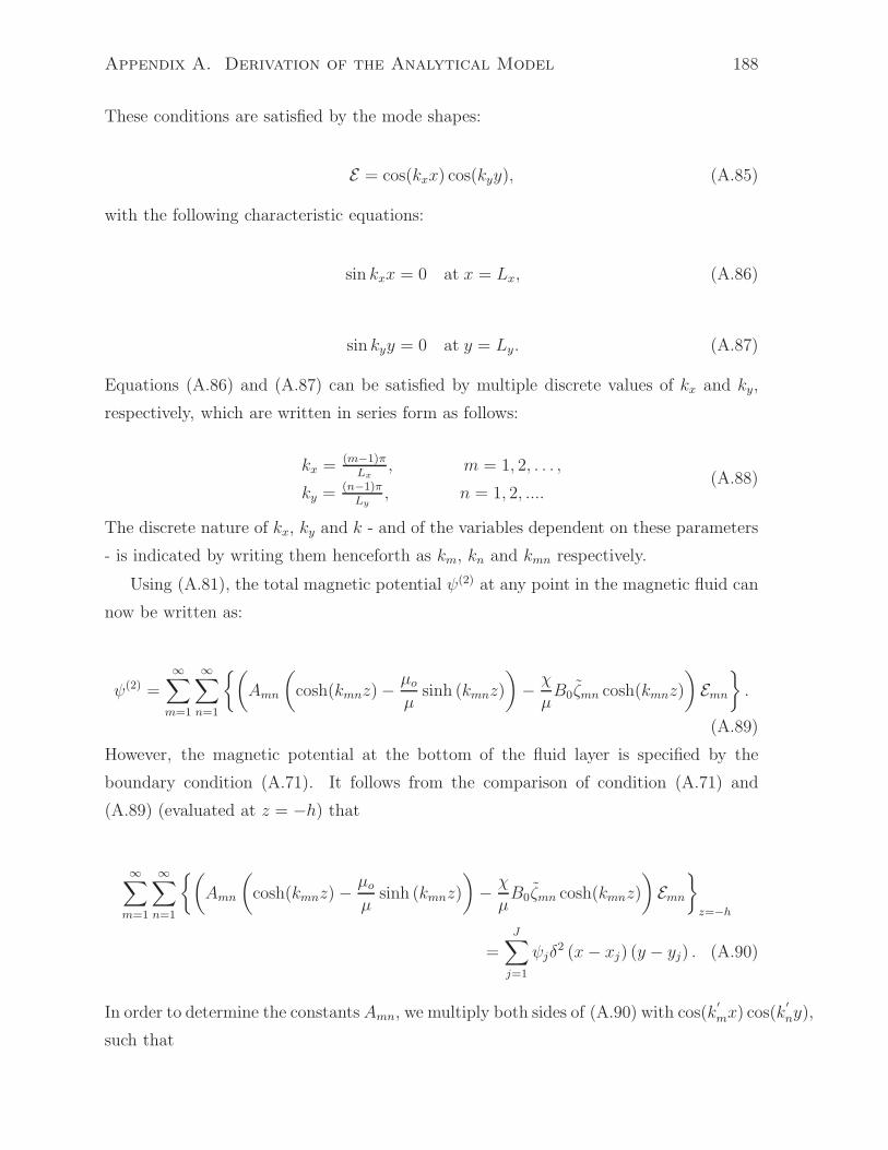
Appendix A. Derivation of the Analytical Model 188
These conditions are satisfied by the mode shapes:
E = cos(kxx) cos(kyy), (A.85)
with the following characteristic equations:
sin kxx = 0 at x = Lx, (A.86)
sin kyy = 0 at y = Ly. (A.87)
Equations (A.86) and (A.87) can be satisfied by multiple discrete values of kx and ky,
respectively, which are written in series form as follows:
kx = (m−1)πLx
, m = 1, 2, . . . ,
ky = (n−1)πLy
, n = 1, 2, ....(A.88)
The discrete nature of kx, ky and k - and of the variables dependent on these parameters
- is indicated by writing them henceforth as km, kn and kmn respectively.
Using (A.81), the total magnetic potential ψ(2) at any point in the magnetic fluid can
now be written as:
ψ(2) =
∞∑
m=1
∞∑
n=1
(
Amn
(
cosh(kmnz) −µoµ
sinh (kmnz)
)
− χ
µB0ζmn cosh(kmnz)
)
Emn
.
(A.89)
However, the magnetic potential at the bottom of the fluid layer is specified by the
boundary condition (A.71). It follows from the comparison of condition (A.71) and
(A.89) (evaluated at z = −h) that
∞∑
m=1
∞∑
n=1
(
Amn
(
cosh(kmnz) −µoµ
sinh (kmnz)
)
− χ
µB0ζmn cosh(kmnz)
)
Emn
z=−h
=J∑
j=1
ψjδ2 (x− xj) (y − yj) . (A.90)
In order to determine the constants Amn, we multiply both sides of (A.90) with cos(k′
mx) cos(k′
ny),
such that

Appendix A. Derivation of the Analytical Model 189
k′m = (m′−1)πLx
, m′ = 1, 2, ...,
k′n = (n′−1)πLy
, n′ = 1, 2, ...,(A.91)
and integrate w.r.t. x and y over the domain 0 < x < Lx, 0 < y < Ly. The orthogonality
of the mode shapes Emn results in
∫ Lx
0cos(kmx) cos(k′mx)dx =
0 m 6= m′,
Lx m = m′ = 1,
Lx/2 m = m′ > 1,
∫ Ly
0cos(kny) cos(k′ny)dy =
0 n 6= n′,
Ly n = n′ = 1,
Ly/2 n = n′ > 1,
(A.92)
which allows to write the constants Amn as:
Amn =1
cosh (kmnh) + µo
µsinh (kmnh)
(χ
µoBo cosh (kmnh) ζmn+
cmcnLxLy
J∑
j=1
ψj cos (kmxj) cos (knyj)
)
, (A.93)
where
cm =
1 for m = 1,
2 for m > 1,
cn =
1 for n = 1,
2 for n > 1.
(A.94)
Substituting Amn from (A.93) into (A.80) and (A.81), the magnetic potentials ψ(1) and
ψ(2) are fully determined thus completing the solution of the Laplace equations (A.50)-
(A.52).
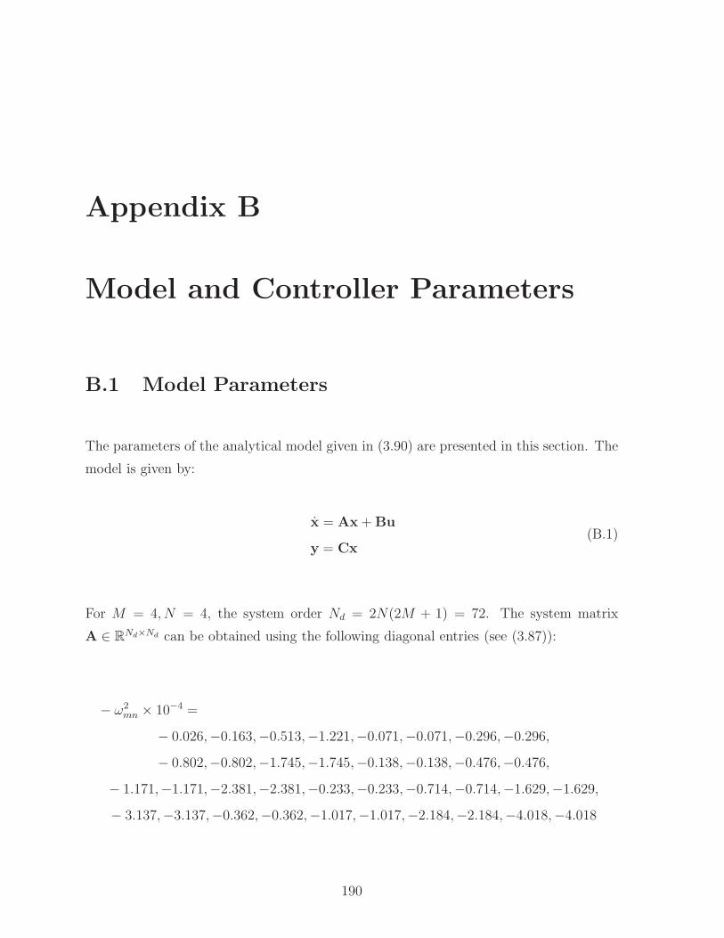
Appendix B
Model and Controller Parameters
B.1 Model Parameters
The parameters of the analytical model given in (3.90) are presented in this section. The
model is given by:
x = Ax + Bu
y = Cx(B.1)
For M = 4, N = 4, the system order Nd = 2N(2M + 1) = 72. The system matrix
A ∈ RNd×Nd can be obtained using the following diagonal entries (see (3.87)):
− ω2mn × 10−4 =
− 0.026,−0.163,−0.513,−1.221,−0.071,−0.071,−0.296,−0.296,
− 0.802,−0.802,−1.745,−1.745,−0.138,−0.138,−0.476,−0.476,
− 1.171,−1.171,−2.381,−2.381,−0.233,−0.233,−0.714,−0.714,−1.629,−1.629,
− 3.137,−3.137,−0.362,−0.362,−1.017,−1.017,−2.184,−2.184,−4.018,−4.018
190

Appendix B. Model and Controller Parameters 191
and
− ω2dmn
× 10−2 =
− 0.138,−0.727,−1.787,−3.318,−0.350,−0.350,−1.174,−1.174,−2.470
− 2.470,−4.236,−4.236,−0.629,−0.629,−1.691,−1.691,−3.222,−3.222
− 5.224,−5.224,−0.971,−0.971,−2.273,−2.273,−4.042,−4.042,−6.280
− 6.280,−1.374,−1.374,−2.921,−2.921,−4.929,−4.929,−7.404,−7.404
The matrices B ∈ RNd×L and C ∈ R
M×Nd, where L and M are the number of inputs and
outputs, respectively, are produced using the following block matrices:
B =
[
B11 B12
B21 B22
]
× 103
C =[
C11 C12 C13 C14 C15
]
The block matrices are given on the following pages.
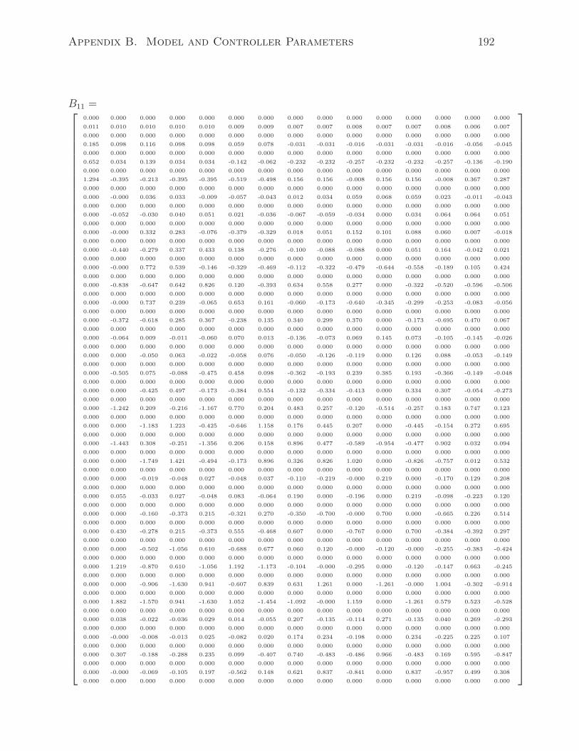
Appendix B. Model and Controller Parameters 192
B11 =
0.000 0.000 0.000 0.000 0.000 0.000 0.000 0.000 0.000 0.000 0.000 0.000 0.000 0.000 0.000
0.011 0.010 0.010 0.010 0.010 0.009 0.009 0.007 0.007 0.008 0.007 0.007 0.008 0.006 0.007
0.000 0.000 0.000 0.000 0.000 0.000 0.000 0.000 0.000 0.000 0.000 0.000 0.000 0.000 0.000
0.185 0.098 0.116 0.098 0.098 0.059 0.078 -0.031 -0.031 -0.016 -0.031 -0.031 -0.016 -0.056 -0.045
0.000 0.000 0.000 0.000 0.000 0.000 0.000 0.000 0.000 0.000 0.000 0.000 0.000 0.000 0.000
0.652 0.034 0.139 0.034 0.034 -0.142 -0.062 -0.232 -0.232 -0.257 -0.232 -0.232 -0.257 -0.136 -0.190
0.000 0.000 0.000 0.000 0.000 0.000 0.000 0.000 0.000 0.000 0.000 0.000 0.000 0.000 0.000
1.294 -0.395 -0.213 -0.395 -0.395 -0.519 -0.498 0.156 0.156 -0.008 0.156 0.156 -0.008 0.367 0.287
0.000 0.000 0.000 0.000 0.000 0.000 0.000 0.000 0.000 0.000 0.000 0.000 0.000 0.000 0.000
0.000 -0.000 0.036 0.033 -0.009 -0.057 -0.043 0.012 0.034 0.059 0.068 0.059 0.023 -0.011 -0.043
0.000 0.000 0.000 0.000 0.000 0.000 0.000 0.000 0.000 0.000 0.000 0.000 0.000 0.000 0.000
0.000 -0.052 -0.030 0.040 0.051 0.021 -0.036 -0.067 -0.059 -0.034 0.000 0.034 0.064 0.064 0.051
0.000 0.000 0.000 0.000 0.000 0.000 0.000 0.000 0.000 0.000 0.000 0.000 0.000 0.000 0.000
0.000 -0.000 0.332 0.283 -0.076 -0.379 -0.329 0.018 0.051 0.152 0.101 0.088 0.060 0.007 -0.018
0.000 0.000 0.000 0.000 0.000 0.000 0.000 0.000 0.000 0.000 0.000 0.000 0.000 0.000 0.000
0.000 -0.440 -0.279 0.337 0.433 0.138 -0.276 -0.100 -0.088 -0.088 0.000 0.051 0.164 -0.042 0.021
0.000 0.000 0.000 0.000 0.000 0.000 0.000 0.000 0.000 0.000 0.000 0.000 0.000 0.000 0.000
0.000 -0.000 0.772 0.539 -0.146 -0.329 -0.469 -0.112 -0.322 -0.479 -0.644 -0.558 -0.189 0.105 0.424
0.000 0.000 0.000 0.000 0.000 0.000 0.000 0.000 0.000 0.000 0.000 0.000 0.000 0.000 0.000
0.000 -0.838 -0.647 0.642 0.826 0.120 -0.393 0.634 0.558 0.277 0.000 -0.322 -0.520 -0.596 -0.506
0.000 0.000 0.000 0.000 0.000 0.000 0.000 0.000 0.000 0.000 0.000 0.000 0.000 0.000 0.000
0.000 -0.000 0.737 0.239 -0.065 0.653 0.161 -0.060 -0.173 -0.640 -0.345 -0.299 -0.253 -0.083 -0.056
0.000 0.000 0.000 0.000 0.000 0.000 0.000 0.000 0.000 0.000 0.000 0.000 0.000 0.000 0.000
0.000 -0.372 -0.618 0.285 0.367 -0.238 0.135 0.340 0.299 0.370 0.000 -0.173 -0.695 0.470 0.067
0.000 0.000 0.000 0.000 0.000 0.000 0.000 0.000 0.000 0.000 0.000 0.000 0.000 0.000 0.000
0.000 -0.064 0.009 -0.011 -0.060 0.070 0.013 -0.136 -0.073 0.069 0.145 0.073 -0.105 -0.145 -0.026
0.000 0.000 0.000 0.000 0.000 0.000 0.000 0.000 0.000 0.000 0.000 0.000 0.000 0.000 0.000
0.000 0.000 -0.050 0.063 -0.022 -0.058 0.076 -0.050 -0.126 -0.119 0.000 0.126 0.088 -0.053 -0.149
0.000 0.000 0.000 0.000 0.000 0.000 0.000 0.000 0.000 0.000 0.000 0.000 0.000 0.000 0.000
0.000 -0.505 0.075 -0.088 -0.475 0.458 0.098 -0.362 -0.193 0.239 0.385 0.193 -0.366 -0.149 -0.048
0.000 0.000 0.000 0.000 0.000 0.000 0.000 0.000 0.000 0.000 0.000 0.000 0.000 0.000 0.000
0.000 0.000 -0.425 0.497 -0.173 -0.384 0.554 -0.132 -0.334 -0.413 0.000 0.334 0.307 -0.054 -0.273
0.000 0.000 0.000 0.000 0.000 0.000 0.000 0.000 0.000 0.000 0.000 0.000 0.000 0.000 0.000
0.000 -1.242 0.209 -0.216 -1.167 0.770 0.204 0.483 0.257 -0.120 -0.514 -0.257 0.183 0.747 0.123
0.000 0.000 0.000 0.000 0.000 0.000 0.000 0.000 0.000 0.000 0.000 0.000 0.000 0.000 0.000
0.000 0.000 -1.183 1.223 -0.425 -0.646 1.158 0.176 0.445 0.207 0.000 -0.445 -0.154 0.272 0.695
0.000 0.000 0.000 0.000 0.000 0.000 0.000 0.000 0.000 0.000 0.000 0.000 0.000 0.000 0.000
0.000 -1.443 0.308 -0.251 -1.356 0.206 0.158 0.896 0.477 -0.589 -0.954 -0.477 0.902 0.032 0.094
0.000 0.000 0.000 0.000 0.000 0.000 0.000 0.000 0.000 0.000 0.000 0.000 0.000 0.000 0.000
0.000 0.000 -1.749 1.421 -0.494 -0.173 0.896 0.326 0.826 1.020 0.000 -0.826 -0.757 0.012 0.532
0.000 0.000 0.000 0.000 0.000 0.000 0.000 0.000 0.000 0.000 0.000 0.000 0.000 0.000 0.000
0.000 0.000 -0.019 -0.048 0.027 -0.048 0.037 -0.110 -0.219 -0.000 0.219 0.000 -0.170 0.129 0.208
0.000 0.000 0.000 0.000 0.000 0.000 0.000 0.000 0.000 0.000 0.000 0.000 0.000 0.000 0.000
0.000 0.055 -0.033 0.027 -0.048 0.083 -0.064 0.190 0.000 -0.196 0.000 0.219 -0.098 -0.223 0.120
0.000 0.000 0.000 0.000 0.000 0.000 0.000 0.000 0.000 0.000 0.000 0.000 0.000 0.000 0.000
0.000 0.000 -0.160 -0.373 0.215 -0.321 0.270 -0.350 -0.700 -0.000 0.700 0.000 -0.665 0.226 0.514
0.000 0.000 0.000 0.000 0.000 0.000 0.000 0.000 0.000 0.000 0.000 0.000 0.000 0.000 0.000
0.000 0.430 -0.278 0.215 -0.373 0.555 -0.468 0.607 0.000 -0.767 0.000 0.700 -0.384 -0.392 0.297
0.000 0.000 0.000 0.000 0.000 0.000 0.000 0.000 0.000 0.000 0.000 0.000 0.000 0.000 0.000
0.000 0.000 -0.502 -1.056 0.610 -0.688 0.677 0.060 0.120 -0.000 -0.120 -0.000 -0.255 -0.383 -0.424
0.000 0.000 0.000 0.000 0.000 0.000 0.000 0.000 0.000 0.000 0.000 0.000 0.000 0.000 0.000
0.000 1.219 -0.870 0.610 -1.056 1.192 -1.173 -0.104 -0.000 -0.295 0.000 -0.120 -0.147 0.663 -0.245
0.000 0.000 0.000 0.000 0.000 0.000 0.000 0.000 0.000 0.000 0.000 0.000 0.000 0.000 0.000
0.000 0.000 -0.906 -1.630 0.941 -0.607 0.839 0.631 1.261 0.000 -1.261 -0.000 1.004 -0.302 -0.914
0.000 0.000 0.000 0.000 0.000 0.000 0.000 0.000 0.000 0.000 0.000 0.000 0.000 0.000 0.000
0.000 1.882 -1.570 0.941 -1.630 1.052 -1.454 -1.092 -0.000 1.159 0.000 -1.261 0.579 0.523 -0.528
0.000 0.000 0.000 0.000 0.000 0.000 0.000 0.000 0.000 0.000 0.000 0.000 0.000 0.000 0.000
0.000 0.038 -0.022 -0.036 0.029 0.014 -0.055 0.207 -0.135 -0.114 0.271 -0.135 0.040 0.269 -0.293
0.000 0.000 0.000 0.000 0.000 0.000 0.000 0.000 0.000 0.000 0.000 0.000 0.000 0.000 0.000
0.000 -0.000 -0.008 -0.013 0.025 -0.082 0.020 0.174 0.234 -0.198 0.000 0.234 -0.225 0.225 0.107
0.000 0.000 0.000 0.000 0.000 0.000 0.000 0.000 0.000 0.000 0.000 0.000 0.000 0.000 0.000
0.000 0.307 -0.188 -0.288 0.235 0.099 -0.407 0.740 -0.483 -0.486 0.966 -0.483 0.169 0.595 -0.847
0.000 0.000 0.000 0.000 0.000 0.000 0.000 0.000 0.000 0.000 0.000 0.000 0.000 0.000 0.000
0.000 -0.000 -0.069 -0.105 0.197 -0.562 0.148 0.621 0.837 -0.841 0.000 0.837 -0.957 0.499 0.308
0.000 0.000 0.000 0.000 0.000 0.000 0.000 0.000 0.000 0.000 0.000 0.000 0.000 0.000 0.000

Appendix B. Model and Controller Parameters 193
B12 =
0.000 0.000 0.000 0.000
0.006 0.006 0.007 0.008
0.000 0.000 0.000 0.000
-0.064 -0.064 -0.045 -0.016
0.000 0.000 0.000 0.000
-0.074 -0.074 -0.190 -0.257
0.000 0.000 0.000 0.000
0.388 0.388 0.287 -0.008
0.000 0.000 0.000 0.000
-0.055 -0.063 -0.058 -0.034
0.000 0.000 0.000 0.000
0.031 0.000 -0.033 -0.059
0.000 0.000 0.000 0.000
0.093 0.107 -0.024 -0.088
0.000 0.000 0.000 0.000
-0.054 -0.000 -0.014 -0.152
0.000 0.000 0.000 0.000
0.423 0.488 0.572 0.277
0.000 0.000 0.000 0.000
-0.244 -0.000 0.330 0.479
0.000 0.000 0.000 0.000
-0.655 -0.756 -0.075 0.370
0.000 0.000 0.000 0.000
0.378 0.000 -0.044 0.640
0.000 0.000 0.000 0.000
0.078 0.155 0.075 -0.069
0.000 0.000 0.000 0.000
-0.134 -0.000 0.131 0.119
0.000 0.000 0.000 0.000
0.018 0.037 0.138 -0.239
0.000 0.000 0.000 0.000
-0.032 -0.000 0.240 0.413
0.000 0.000 0.000 0.000
-0.388 -0.775 -0.353 0.120
0.000 0.000 0.000 0.000
0.671 0.000 -0.611 -0.207
0.000 0.000 0.000 0.000
0.225 0.450 -0.270 0.589
0.000 0.000 0.000 0.000
-0.390 -0.000 -0.468 -1.020
0.000 0.000 0.000 0.000
0.000 -0.270 -0.000 0.196
0.000 0.000 0.000 0.000
0.270 0.000 -0.240 0.000
0.000 0.000 0.000 0.000
0.000 -0.287 -0.000 0.767
0.000 0.000 0.000 0.000
0.287 0.000 -0.593 0.000
0.000 0.000 0.000 0.000
-0.000 0.910 0.000 0.295
0.000 0.000 0.000 0.000
-0.910 -0.000 0.490 0.000
0.000 0.000 0.000 0.000
-0.000 0.029 0.000 -1.159
0.000 0.000 0.000 0.000
-0.029 -0.000 1.055 -0.000
0.000 0.000 0.000 0.000
-0.192 0.384 -0.156 -0.114
0.000 0.000 0.000 0.000
-0.333 -0.000 0.270 -0.198
0.000 0.000 0.000 0.000
-0.299 0.599 -0.451 -0.486
0.000 0.000 0.000 0.000
-0.519 -0.000 0.781 -0.841
0.000 0.000 0.000 0.000

Appendix B. Model and Controller Parameters 194
B21 =
0.000 0.967 -0.648 -0.909 0.741 0.248 -1.156 0.315 -0.206 -0.434 0.411 -0.206 0.151 -0.401 0.073
0.000 0.000 0.000 0.000 0.000 0.000 0.000 0.000 0.000 0.000 0.000 0.000 0.000 0.000 0.000
0.000 -0.000 -0.236 -0.331 0.622 -1.405 0.421 0.264 0.356 -0.752 0.000 0.356 -0.855 -0.337 -0.027
0.000 0.000 0.000 0.000 0.000 0.000 0.000 0.000 0.000 0.000 0.000 0.000 0.000 0.000 0.000
0.000 1.769 -1.339 -1.663 1.355 0.310 -1.800 -0.916 0.598 0.372 -1.196 0.598 -0.129 -0.816 1.230
0.000 0.000 0.000 0.000 0.000 0.000 0.000 0.000 0.000 0.000 0.000 0.000 0.000 0.000 0.000
0.000 -0.000 -0.488 -0.605 1.137 -1.756 0.655 -0.768 -1.035 0.644 0.000 -1.035 0.732 -0.685 -0.448
B22 =
0.429 -0.857 0.039 -0.434
0.000 0.000 0.000 0.000
0.742 0.000 -0.067 -0.752
0.000 0.000 0.000 0.000
0.272 -0.543 0.654 0.372
0.000 0.000 0.000 0.000
0.471 0.000 -1.133 0.644
C11 =
21.000 0.000 21.000 0.000 21.000 0.000 21.000 0.000 0.000 0.000 0.000 0.000 0.000 0.000 0.000
18.896 0.000 11.075 0.000 1.080 0.000 -6.406 0.000 -0.000 0.000 -9.388 0.000 -0.000 0.000 -12.215
19.379 0.000 13.153 0.000 4.469 0.000 -3.459 0.000 6.496 0.000 -5.451 0.000 9.222 0.000 -7.738
18.896 0.000 11.075 0.000 1.080 0.000 -6.406 0.000 6.035 0.000 7.192 0.000 7.852 0.000 9.358
18.896 0.000 11.075 0.000 1.080 0.000 -6.406 0.000 -1.630 0.000 9.246 0.000 -2.121 0.000 12.030
17.760 0.000 6.651 0.000 -4.588 0.000 -8.417 0.000 -10.201 0.000 3.713 0.000 -10.512 0.000 3.826
18.355 0.000 8.890 0.000 -1.994 0.000 -8.085 0.000 -7.801 0.000 -6.546 0.000 -9.134 0.000 -7.664
14.069 0.000 -3.536 0.000 -7.482 0.000 2.536 0.000 2.118 0.000 -12.010 0.000 0.489 0.000 -2.774
14.069 0.000 -3.536 0.000 -7.482 0.000 2.536 0.000 6.098 0.000 -10.561 0.000 1.408 0.000 -2.439
14.891 0.000 -1.794 0.000 -8.281 0.000 -0.124 0.000 10.572 0.000 -6.104 0.000 4.207 0.000 -2.429
14.069 0.000 -3.536 0.000 -7.482 0.000 2.536 0.000 12.195 0.000 0.000 0.000 2.816 0.000 0.000
14.069 0.000 -3.536 0.000 -7.482 0.000 2.536 0.000 10.561 0.000 6.098 0.000 2.439 0.000 1.408
14.891 0.000 -1.794 0.000 -8.281 0.000 -0.124 0.000 4.175 0.000 11.471 0.000 1.662 0.000 4.565
12.325 0.000 -6.307 0.000 -4.380 0.000 5.949 0.000 -2.042 0.000 11.579 0.000 0.207 0.000 -1.172
13.212 0.000 -5.050 0.000 -6.136 0.000 4.651 0.000 -7.742 0.000 9.226 0.000 -0.495 0.000 0.590
11.412 0.000 -7.285 0.000 -2.372 0.000 6.291 0.000 -9.822 0.000 5.670 0.000 2.580 0.000 -1.489
11.412 0.000 -7.285 0.000 -2.372 0.000 6.291 0.000 -11.341 0.000 0.000 0.000 2.979 0.000 -0.000
13.212 0.000 -5.050 0.000 -6.136 0.000 4.651 0.000 -10.431 0.000 -6.022 0.000 -0.667 0.000 -0.385
14.891 0.000 -1.794 0.000 -8.281 0.000 -0.124 0.000 -6.104 0.000 -10.572 0.000 -2.429 0.000 -4.207
C12 =
21.000 0.000 21.000 0.000 0.000 0.000 0.000 0.000 0.000 0.000 0.000 0.000 0.000 0.000 0.000
1.080 0.000 -6.406 0.000 -0.000 0.000 -9.388 0.000 -0.000 0.000 -12.215 0.000 -0.000 0.000 -9.190
4.469 0.000 -3.459 0.000 6.496 0.000 -5.451 0.000 9.222 0.000 -7.738 0.000 8.457 0.000 -7.096
1.080 0.000 -6.406 0.000 6.035 0.000 7.192 0.000 7.852 0.000 9.358 0.000 5.907 0.000 7.040
1.080 0.000 -6.406 0.000 -1.630 0.000 9.246 0.000 -2.121 0.000 12.030 0.000 -1.596 0.000 9.050
-4.588 0.000 -8.417 0.000 -10.201 0.000 3.713 0.000 -10.512 0.000 3.826 0.000 -3.610 0.000 1.314
-1.994 0.000 -8.085 0.000 -7.801 0.000 -6.546 0.000 -9.134 0.000 -7.664 0.000 -5.138 0.000 -4.312
-7.482 0.000 2.536 0.000 2.118 0.000 -12.010 0.000 0.489 0.000 -2.774 0.000 -1.225 0.000 6.949
-7.482 0.000 2.536 0.000 6.098 0.000 -10.561 0.000 1.408 0.000 -2.439 0.000 -3.528 0.000 6.111
-8.281 0.000 -0.124 0.000 10.572 0.000 -6.104 0.000 4.207 0.000 -2.429 0.000 -5.251 0.000 3.032
-7.482 0.000 2.536 0.000 12.195 0.000 0.000 0.000 2.816 0.000 0.000 0.000 -7.057 0.000 0.000
-7.482 0.000 2.536 0.000 10.561 0.000 6.098 0.000 2.439 0.000 1.408 0.000 -6.111 0.000 -3.528
-8.281 0.000 -0.124 0.000 4.175 0.000 11.471 0.000 1.662 0.000 4.565 0.000 -2.074 0.000 -5.698
-4.380 0.000 5.949 0.000 -2.042 0.000 11.579 0.000 0.207 0.000 -1.172 0.000 1.152 0.000 -6.534
-6.136 0.000 4.651 0.000 -7.742 0.000 9.226 0.000 -0.495 0.000 0.590 0.000 4.652 0.000 -5.544
-2.372 0.000 6.291 0.000 -9.822 0.000 5.670 0.000 2.580 0.000 -1.489 0.000 4.637 0.000 -2.677
-2.372 0.000 6.291 0.000 -11.341 0.000 0.000 0.000 2.979 0.000 -0.000 0.000 5.354 0.000 -0.000
-6.136 0.000 4.651 0.000 -10.431 0.000 -6.022 0.000 -0.667 0.000 -0.385 0.000 6.268 0.000 3.619
-8.281 0.000 -0.124 0.000 -6.104 0.000 -10.572 0.000 -2.429 0.000 -4.207 0.000 3.032 0.000 5.251

Appendix B. Model and Controller Parameters 195
C13 =
0.000 0.000 0.000 0.000 0.000 0.000 0.000 0.000 0.000 0.000 0.000 0.000 0.000 0.000 0.000
-0.000 0.000 -9.388 0.000 -0.000 0.000 -12.215 0.000 -0.000 0.000 -9.190 0.000 -0.000 0.000 -2.418
6.496 0.000 -5.451 0.000 9.222 0.000 -7.738 0.000 8.457 0.000 -7.096 0.000 4.785 0.000 -4.015
6.035 0.000 7.192 0.000 7.852 0.000 9.358 0.000 5.907 0.000 7.040 0.000 1.554 0.000 1.853
-1.630 0.000 9.246 0.000 -2.121 0.000 12.030 0.000 -1.596 0.000 9.050 0.000 -0.420 0.000 2.382
-10.201 0.000 3.713 0.000 -10.512 0.000 3.826 0.000 -3.610 0.000 1.314 0.000 4.238 0.000 -1.543
-7.801 0.000 -6.546 0.000 -9.134 0.000 -7.664 0.000 -5.138 0.000 -4.312 0.000 1.045 0.000 0.877
2.118 0.000 -12.010 0.000 0.489 0.000 -2.774 0.000 -1.225 0.000 6.949 0.000 -0.389 0.000 2.207
6.098 0.000 -10.561 0.000 1.408 0.000 -2.439 0.000 -3.528 0.000 6.111 0.000 -1.121 0.000 1.941
10.572 0.000 -6.104 0.000 4.207 0.000 -2.429 0.000 -5.251 0.000 3.032 0.000 -4.158 0.000 2.401
12.195 0.000 0.000 0.000 2.816 0.000 0.000 0.000 -7.057 0.000 0.000 0.000 -2.241 0.000 0.000
10.561 0.000 6.098 0.000 2.439 0.000 1.408 0.000 -6.111 0.000 -3.528 0.000 -1.941 0.000 -1.121
4.175 0.000 11.471 0.000 1.662 0.000 4.565 0.000 -2.074 0.000 -5.698 0.000 -1.642 0.000 -4.512
-2.042 0.000 11.579 0.000 0.207 0.000 -1.172 0.000 1.152 0.000 -6.534 0.000 -0.538 0.000 3.050
-7.742 0.000 9.226 0.000 -0.495 0.000 0.590 0.000 4.652 0.000 -5.544 0.000 -0.363 0.000 0.433
-9.822 0.000 5.670 0.000 2.580 0.000 -1.489 0.000 4.637 0.000 -2.677 0.000 -4.252 0.000 2.455
-11.341 0.000 0.000 0.000 2.979 0.000 -0.000 0.000 5.354 0.000 -0.000 0.000 -4.910 0.000 0.000
-10.431 0.000 -6.022 0.000 -0.667 0.000 -0.385 0.000 6.268 0.000 3.619 0.000 -0.490 0.000 -0.283
-6.104 0.000 -10.572 0.000 -2.429 0.000 -4.207 0.000 3.032 0.000 5.251 0.000 2.401 0.000 4.158
C14 =
0.000 0.000 0.000 0.000 0.000 0.000 0.000 0.000 0.000 0.000 0.000 0.000 0.000 0.000 0.000
-0.000 0.000 -12.215 0.000 -0.000 0.000 -9.190 0.000 -0.000 0.000 -2.418 0.000 -4.198 0.000 0.000
9.222 0.000 -7.738 0.000 8.457 0.000 -7.096 0.000 4.785 0.000 -4.015 0.000 0.580 0.000 -3.287
7.852 0.000 9.358 0.000 5.907 0.000 7.040 0.000 1.554 0.000 1.853 0.000 -0.729 0.000 4.134
-2.121 0.000 12.030 0.000 -1.596 0.000 9.050 0.000 -0.420 0.000 2.382 0.000 -3.944 0.000 -1.436
-10.512 0.000 3.826 0.000 -3.610 0.000 1.314 0.000 4.238 0.000 -1.543 0.000 4.579 0.000 -3.843
-9.134 0.000 -7.664 0.000 -5.138 0.000 -4.312 0.000 1.045 0.000 0.877 0.000 0.883 0.000 5.009
0.489 0.000 -2.774 0.000 -1.225 0.000 6.949 0.000 -0.389 0.000 2.207 0.000 -8.980 0.000 -3.268
1.408 0.000 -2.439 0.000 -3.528 0.000 6.111 0.000 -1.121 0.000 1.941 0.000 -4.778 0.000 -8.276
4.207 0.000 -2.429 0.000 -5.251 0.000 3.032 0.000 -4.158 0.000 2.401 0.000 4.520 0.000 -7.828
2.816 0.000 0.000 0.000 -7.057 0.000 0.000 0.000 -2.241 0.000 0.000 0.000 9.556 0.000 0.000
2.439 0.000 1.408 0.000 -6.111 0.000 -3.528 0.000 -1.941 0.000 -1.121 0.000 4.778 0.000 8.276
1.662 0.000 4.565 0.000 -2.074 0.000 -5.698 0.000 -1.642 0.000 -4.512 0.000 -6.924 0.000 5.810
0.207 0.000 -1.172 0.000 1.152 0.000 -6.534 0.000 -0.538 0.000 3.050 0.000 -9.544 0.000 -3.474
-0.495 0.000 0.590 0.000 4.652 0.000 -5.544 0.000 -0.363 0.000 0.433 0.000 -1.725 0.000 -9.783
2.580 0.000 -1.489 0.000 4.637 0.000 -2.677 0.000 -4.252 0.000 2.455 0.000 5.107 0.000 -8.846
2.979 0.000 -0.000 0.000 5.354 0.000 -0.000 0.000 -4.910 0.000 0.000 0.000 10.214 0.000 -0.000
-0.667 0.000 -0.385 0.000 6.268 0.000 3.619 0.000 -0.490 0.000 -0.283 0.000 4.967 0.000 8.603
-2.429 0.000 -4.207 0.000 3.032 0.000 5.251 0.000 2.401 0.000 4.158 0.000 -4.520 0.000 7.828
C15 =
0.000 0.000 0.000 0.000 0.000 0.000 0.000 0.000 0.000 0.000 0.000 0.000
2.636 0.000 -0.000 0.000 5.371 0.000 -0.000 0.000 7.750 0.000 -0.000 0.000
-1.620 0.000 -0.590 0.000 -3.596 0.000 -1.309 0.000 -5.867 0.000 -2.136 0.000
-2.477 0.000 -0.902 0.000 -5.047 0.000 -1.837 0.000 -7.283 0.000 -2.651 0.000
2.019 0.000 1.695 0.000 4.114 0.000 3.452 0.000 5.937 0.000 4.982 0.000
0.851 0.000 -4.828 0.000 1.376 0.000 -7.801 0.000 1.357 0.000 -7.693 0.000
-3.496 0.000 1.272 0.000 -6.417 0.000 2.335 0.000 -7.885 0.000 2.870 0.000
6.364 0.000 5.340 0.000 1.750 0.000 1.468 0.000 -4.012 0.000 -3.366 0.000
-4.154 0.000 7.194 0.000 -1.142 0.000 1.978 0.000 2.618 0.000 -4.535 0.000
-4.175 0.000 -7.231 0.000 -2.411 0.000 -4.176 0.000 1.628 0.000 2.820 0.000
8.307 0.000 0.000 0.000 2.284 0.000 0.000 0.000 -5.237 0.000 0.000 0.000
-4.154 0.000 7.194 0.000 -1.142 0.000 1.978 0.000 2.618 0.000 -4.535 0.000
1.450 0.000 -8.223 0.000 0.837 0.000 -4.749 0.000 -0.565 0.000 3.207 0.000
5.115 0.000 4.292 0.000 -2.229 0.000 -1.871 0.000 -3.574 0.000 -2.999 0.000
-7.281 0.000 2.650 0.000 0.405 0.000 -0.148 0.000 5.387 0.000 -1.961 0.000
-2.574 0.000 -4.458 0.000 2.380 0.000 4.122 0.000 1.190 0.000 2.062 0.000
5.148 0.000 -0.000 0.000 -4.760 0.000 0.000 0.000 -2.381 0.000 0.000 0.000
-3.874 0.000 6.711 0.000 0.216 0.000 -0.374 0.000 2.866 0.000 -4.964 0.000
-4.175 0.000 -7.231 0.000 -2.411 0.000 -4.176 0.000 1.628 0.000 2.820 0.000

Appendix B. Model and Controller Parameters 196
B.2 Mixed Sensitivity H∞ Controller Parameters
The parameters of the mixed sensitivity controller (5.63) designed in section 5.4 are
presented in this section. The controller is given by:
∑
K∞
:
x(k + 1) = Acx(k) + Bce(k)
u(k) = Ccx(k) + Dce(k)(B.2)
The system matrices Ac, Bc, Cc and Dc are given below.
Ac =[
A11 A12 A13
]
× 10−1
Bc =[
B11 B12
]
× 104
Cc =[
C11 C12 C13
]
× 10−2
Dc =[
D11 D12
]
× 10−1
The block matrices are given on the following pages.

Appendix B. Model and Controller Parameters 197
A11 =
-5.408 -4.534 0.112 -0.305 -0.714 -0.029 -0.082 0.000 0.000 0.000 0.000 0.000 0.000 0.000 0.000
4.851 0.306 -0.330 2.223 -2.229 -0.077 -0.607 0.000 0.000 0.000 0.000 0.000 0.000 0.000 0.000
-0.281 0.250 -1.640 0.752 -1.475 3.765 -0.135 0.000 0.000 0.000 0.000 0.000 0.000 0.000 0.000
0.498 -0.565 -0.788 -2.007 3.810 1.022 0.773 0.000 0.000 0.000 0.000 0.000 0.000 0.000 0.000
0.529 0.197 1.414 -6.903 4.024 0.658 -1.248 0.000 0.000 0.000 0.000 0.000 0.000 0.000 0.000
0.006 -0.022 -4.517 -1.145 -0.478 2.774 -0.334 0.000 0.000 0.000 0.000 0.000 0.000 0.000 0.000
0.127 -1.050 0.102 -0.345 -0.580 0.117 7.995 0.000 0.000 0.000 0.000 0.000 0.000 0.000 0.000
0.000 0.000 0.000 0.000 0.000 0.000 0.000 -16.316 0.771 -0.533 0.117 0.091 0.055 0.076 -0.251
0.000 0.000 0.000 0.000 0.000 0.000 0.000 0.000 -18.323 -0.379 0.227 -0.019 0.047 -0.072 -0.234
0.000 0.000 0.000 0.000 0.000 0.000 0.000 0.000 0.000 -19.613 -0.177 0.121 -0.180 -0.049 0.218
0.000 0.000 0.000 0.000 0.000 0.000 0.000 0.000 0.000 0.000 -21.034 0.045 0.019 -0.038 -0.017
0.000 0.000 0.000 0.000 0.000 0.000 0.000 0.000 0.000 0.000 0.000 -25.619 0.169 -0.180 -0.239
0.000 0.000 0.000 0.000 0.000 0.000 0.000 0.000 0.000 0.000 0.000 0.000 -25.163 -0.584 -0.199
0.000 0.000 0.000 0.000 0.000 0.000 0.000 0.000 0.000 0.000 0.000 0.000 0.000 -24.563 -0.400
0.000 0.000 0.000 0.000 0.000 0.000 0.000 0.000 0.000 0.000 0.000 0.000 0.000 0.774 -24.563
0.000 0.000 0.000 0.000 0.000 0.000 0.000 0.000 0.000 0.000 0.000 0.000 0.000 0.000 0.000
0.000 0.000 0.000 0.000 0.000 0.000 0.000 0.000 0.000 0.000 0.000 0.000 0.000 0.000 0.000
0.000 0.000 0.000 0.000 0.000 0.000 0.000 0.000 0.000 0.000 0.000 0.000 0.000 0.000 0.000
0.000 0.000 0.000 0.000 0.000 0.000 0.000 0.000 0.000 0.000 0.000 0.000 0.000 0.000 0.000
0.000 0.000 0.000 0.000 0.000 0.000 0.000 0.000 0.000 0.000 0.000 0.000 0.000 0.000 0.000
0.000 0.000 0.000 0.000 0.000 0.000 0.000 0.000 0.000 0.000 0.000 0.000 0.000 0.000 0.000
0.000 0.000 0.000 0.000 0.000 0.000 0.000 0.000 0.000 0.000 0.000 0.000 0.000 0.000 0.000
0.000 0.000 0.000 0.000 0.000 0.000 0.000 0.000 0.000 0.000 0.000 0.000 0.000 0.000 0.000
0.000 0.000 0.000 0.000 0.000 0.000 0.000 0.000 0.000 0.000 0.000 0.000 0.000 0.000 0.000
0.000 0.000 0.000 0.000 0.000 0.000 0.000 0.000 0.000 0.000 0.000 0.000 0.000 0.000 0.000
0.000 0.000 0.000 0.000 0.000 0.000 0.000 0.000 0.000 0.000 0.000 0.000 0.000 0.000 0.000
0.000 0.000 0.000 0.000 0.000 0.000 0.000 0.000 0.000 0.000 0.000 0.000 0.000 0.000 0.000
0.000 0.000 0.000 0.000 0.000 0.000 0.000 0.000 0.000 0.000 0.000 0.000 0.000 0.000 0.000
0.000 0.000 0.000 0.000 0.000 0.000 0.000 0.000 0.000 0.000 0.000 0.000 0.000 0.000 0.000
0.000 0.000 0.000 0.000 0.000 0.000 0.000 0.000 0.000 0.000 0.000 0.000 0.000 0.000 0.000
0.000 0.000 0.000 0.000 0.000 0.000 0.000 0.000 0.000 0.000 0.000 0.000 0.000 0.000 0.000
0.000 0.000 0.000 0.000 0.000 0.000 0.000 0.000 0.000 0.000 0.000 0.000 0.000 0.000 0.000
0.000 0.000 0.000 0.000 0.000 0.000 0.000 0.000 0.000 0.000 0.000 0.000 0.000 0.000 0.000
0.000 0.000 0.000 0.000 0.000 0.000 0.000 0.000 0.000 0.000 0.000 0.000 0.000 0.000 0.000
0.000 0.000 0.000 0.000 0.000 0.000 0.000 0.000 0.000 0.000 0.000 0.000 0.000 0.000 0.000
0.000 0.000 0.000 0.000 0.000 0.000 0.000 0.000 0.000 0.000 0.000 0.000 0.000 0.000 0.000
0.000 0.000 0.000 0.000 0.000 0.000 0.000 0.000 0.000 0.000 0.000 0.000 0.000 0.000 0.000
0.000 0.000 0.000 0.000 0.000 0.000 0.000 0.000 0.000 0.000 0.000 0.000 0.000 0.000 0.000
0.000 0.000 0.000 0.000 0.000 0.000 0.000 0.000 0.000 0.000 0.000 0.000 0.000 0.000 0.000
0.000 0.000 0.000 0.000 0.000 0.000 0.000 0.000 0.000 0.000 0.000 0.000 0.000 0.000 0.000
0.000 0.000 0.000 0.000 0.000 0.000 0.000 0.000 0.000 0.000 0.000 0.000 0.000 0.000 0.000
0.000 0.000 0.000 0.000 0.000 0.000 0.000 0.000 0.000 0.000 0.000 0.000 0.000 0.000 0.000

Appendix B. Model and Controller Parameters 198
A12 =
0.112 -0.305 -0.714 -0.029 -0.082 0.000 0.000 0.000 0.000 0.000 0.000 0.000 0.000 0.000 0.000
-0.330 2.223 -2.229 -0.077 -0.607 0.000 0.000 0.000 0.000 0.000 0.000 0.000 0.000 0.000 0.000
-1.640 0.752 -1.475 3.765 -0.135 0.000 0.000 0.000 0.000 0.000 0.000 0.000 0.000 0.000 0.000
-0.788 -2.007 3.810 1.022 0.773 0.000 0.000 0.000 0.000 0.000 0.000 0.000 0.000 0.000 0.000
1.414 -6.903 4.024 0.658 -1.248 0.000 0.000 0.000 0.000 0.000 0.000 0.000 0.000 0.000 0.000
-4.517 -1.145 -0.478 2.774 -0.334 0.000 0.000 0.000 0.000 0.000 0.000 0.000 0.000 0.000 0.000
0.102 -0.345 -0.580 0.117 7.995 0.000 0.000 0.000 0.000 0.000 0.000 0.000 0.000 0.000 0.000
0.000 0.000 0.000 0.000 0.000 -16.316 0.771 -0.533 0.117 0.091 0.055 0.076 -0.251 -0.116 -0.125
0.000 0.000 0.000 0.000 0.000 0.000 -18.323 -0.379 0.227 -0.019 0.047 -0.072 -0.234 -0.231 0.332
0.000 0.000 0.000 0.000 0.000 0.000 0.000 -19.613 -0.177 0.121 -0.180 -0.049 0.218 0.051 -0.097
0.000 0.000 0.000 0.000 0.000 0.000 0.000 0.000 -21.034 0.045 0.019 -0.038 -0.017 -0.045 0.066
0.000 0.000 0.000 0.000 0.000 0.000 0.000 0.000 0.000 -25.619 0.169 -0.180 -0.239 -0.006 0.044
0.000 0.000 0.000 0.000 0.000 0.000 0.000 0.000 0.000 0.000 -25.163 -0.584 -0.199 -0.082 -0.112
0.000 0.000 0.000 0.000 0.000 0.000 0.000 0.000 0.000 0.000 0.000 -24.563 -0.400 -0.147 0.049
0.000 0.000 0.000 0.000 0.000 0.000 0.000 0.000 0.000 0.000 0.000 0.774 -24.563 0.098 -0.119
0.000 0.000 0.000 0.000 0.000 0.000 0.000 0.000 0.000 0.000 0.000 0.000 0.000 -21.845 -0.051
0.000 0.000 0.000 0.000 0.000 0.000 0.000 0.000 0.000 0.000 0.000 0.000 0.000 0.000 -22.099
0.000 0.000 0.000 0.000 0.000 0.000 0.000 0.000 0.000 0.000 0.000 0.000 0.000 0.000 0.000
0.000 0.000 0.000 0.000 0.000 0.000 0.000 0.000 0.000 0.000 0.000 0.000 0.000 0.000 0.000
0.000 0.000 0.000 0.000 0.000 0.000 0.000 0.000 0.000 0.000 0.000 0.000 0.000 0.000 0.000
0.000 0.000 0.000 0.000 0.000 0.000 0.000 0.000 0.000 0.000 0.000 0.000 0.000 0.000 0.000
0.000 0.000 0.000 0.000 0.000 0.000 0.000 0.000 0.000 0.000 0.000 0.000 0.000 0.000 0.000
0.000 0.000 0.000 0.000 0.000 0.000 0.000 0.000 0.000 0.000 0.000 0.000 0.000 0.000 0.000
0.000 0.000 0.000 0.000 0.000 0.000 0.000 0.000 0.000 0.000 0.000 0.000 0.000 0.000 0.000
0.000 0.000 0.000 0.000 0.000 0.000 0.000 0.000 0.000 0.000 0.000 0.000 0.000 0.000 0.000
0.000 0.000 0.000 0.000 0.000 0.000 0.000 0.000 0.000 0.000 0.000 0.000 0.000 0.000 0.000
0.000 0.000 0.000 0.000 0.000 0.000 0.000 0.000 0.000 0.000 0.000 0.000 0.000 0.000 0.000
0.000 0.000 0.000 0.000 0.000 0.000 0.000 0.000 0.000 0.000 0.000 0.000 0.000 0.000 0.000
0.000 0.000 0.000 0.000 0.000 0.000 0.000 0.000 0.000 0.000 0.000 0.000 0.000 0.000 0.000
0.000 0.000 0.000 0.000 0.000 0.000 0.000 0.000 0.000 0.000 0.000 0.000 0.000 0.000 0.000
0.000 0.000 0.000 0.000 0.000 0.000 0.000 0.000 0.000 0.000 0.000 0.000 0.000 0.000 0.000
0.000 0.000 0.000 0.000 0.000 0.000 0.000 0.000 0.000 0.000 0.000 0.000 0.000 0.000 0.000
0.000 0.000 0.000 0.000 0.000 0.000 0.000 0.000 0.000 0.000 0.000 0.000 0.000 0.000 0.000
0.000 0.000 0.000 0.000 0.000 0.000 0.000 0.000 0.000 0.000 0.000 0.000 0.000 0.000 0.000
0.000 0.000 0.000 0.000 0.000 0.000 0.000 0.000 0.000 0.000 0.000 0.000 0.000 0.000 0.000
0.000 0.000 0.000 0.000 0.000 0.000 0.000 0.000 0.000 0.000 0.000 0.000 0.000 0.000 0.000
0.000 0.000 0.000 0.000 0.000 0.000 0.000 0.000 0.000 0.000 0.000 0.000 0.000 0.000 0.000
0.000 0.000 0.000 0.000 0.000 0.000 0.000 0.000 0.000 0.000 0.000 0.000 0.000 0.000 0.000
0.000 0.000 0.000 0.000 0.000 0.000 0.000 0.000 0.000 0.000 0.000 0.000 0.000 0.000 0.000
0.000 0.000 0.000 0.000 0.000 0.000 0.000 0.000 0.000 0.000 0.000 0.000 0.000 0.000 0.000
0.000 0.000 0.000 0.000 0.000 0.000 0.000 0.000 0.000 0.000 0.000 0.000 0.000 0.000 0.000
0.000 0.000 0.000 0.000 0.000 0.000 0.000 0.000 0.000 0.000 0.000 0.000 0.000 0.000 0.000

Appendix B. Model and Controller Parameters 199
A13 =
0.000 0.000 0.000 0.000 0.000 0.000 0.000 0.000 0.000 0.000 0.000 0.000
0.000 0.000 0.000 0.000 0.000 0.000 0.000 0.000 0.000 0.000 0.000 0.000
0.000 0.000 0.000 0.000 0.000 0.000 0.000 0.000 0.000 0.000 0.000 0.000
0.000 0.000 0.000 0.000 0.000 0.000 0.000 0.000 0.000 0.000 0.000 0.000
0.000 0.000 0.000 0.000 0.000 0.000 0.000 0.000 0.000 0.000 0.000 0.000
0.000 0.000 0.000 0.000 0.000 0.000 0.000 0.000 0.000 0.000 0.000 0.000
0.000 0.000 0.000 0.000 0.000 0.000 0.000 0.000 0.000 0.000 0.000 0.000
0.000 0.000 0.000 0.000 0.000 0.000 0.000 0.000 0.000 0.000 0.000 0.000
0.000 0.000 0.000 0.000 0.000 0.000 0.000 0.000 0.000 0.000 0.000 0.000
0.000 0.000 0.000 0.000 0.000 0.000 0.000 0.000 0.000 0.000 0.000 0.000
0.000 0.000 0.000 0.000 0.000 0.000 0.000 0.000 0.000 0.000 0.000 0.000
0.000 0.000 0.000 0.000 0.000 0.000 0.000 0.000 0.000 0.000 0.000 0.000
0.000 0.000 0.000 0.000 0.000 0.000 0.000 0.000 0.000 0.000 0.000 0.000
0.000 0.000 0.000 0.000 0.000 0.000 0.000 0.000 0.000 0.000 0.000 0.000
0.000 0.000 0.000 0.000 0.000 0.000 0.000 0.000 0.000 0.000 0.000 0.000
0.000 0.000 0.000 0.000 0.000 0.000 0.000 0.000 0.000 0.000 0.000 0.000
0.000 0.000 0.000 0.000 0.000 0.000 0.000 0.000 0.000 0.000 0.000 0.000
0.000 0.000 0.000 0.000 0.000 0.000 0.000 0.000 0.000 0.000 0.000 0.000
0.000 0.000 0.000 0.000 0.000 0.000 0.000 0.000 0.000 0.000 0.000 0.000
0.000 0.000 0.000 0.000 0.000 0.000 0.000 0.000 0.000 0.000 0.000 0.000
0.000 0.000 0.000 0.000 0.000 0.000 0.000 0.000 0.000 0.000 0.000 0.000
0.000 0.000 0.000 0.000 0.000 0.000 0.000 0.000 0.000 0.000 0.000 0.000
0.000 0.000 0.000 0.000 0.000 0.000 0.000 0.000 0.000 0.000 0.000 0.000
0.000 0.000 0.000 0.000 0.000 0.000 0.000 0.000 0.000 0.000 0.000 0.000
0.000 0.000 0.000 0.000 0.000 0.000 0.000 0.000 0.000 0.000 0.000 0.000
0.000 0.000 0.000 0.000 0.000 0.000 0.000 0.000 0.000 0.000 0.000 0.000
0.000 0.000 0.000 0.000 0.000 0.000 0.000 0.000 0.000 0.000 0.000 0.000
0.000 0.000 0.000 0.000 0.000 0.000 0.000 0.000 0.000 0.000 0.000 0.000
0.000 0.000 0.000 0.000 0.000 0.000 0.000 0.000 0.000 0.000 0.000 0.000
0.000 0.000 0.000 0.000 0.000 0.000 0.000 0.000 0.000 0.000 0.000 0.000
10.000 0.000 0.000 0.000 0.000 0.000 0.000 0.000 0.000 0.000 0.000 0.000
0.000 10.000 0.000 0.000 0.000 0.000 0.000 0.000 0.000 0.000 0.000 0.000
0.000 0.000 10.000 0.000 0.000 0.000 0.000 0.000 0.000 0.000 0.000 0.000
0.000 0.000 -0.000 10.000 0.000 0.000 0.000 0.000 0.000 0.000 0.000 0.000
0.000 0.000 0.000 0.000 10.000 0.000 0.000 0.000 0.000 0.000 0.000 0.000
0.000 0.000 0.000 0.000 -0.000 10.000 0.000 0.000 0.000 0.000 0.000 0.000
0.000 0.000 0.000 0.000 0.000 0.000 10.000 0.000 0.000 0.000 0.000 0.000
0.000 0.000 0.000 0.000 0.000 0.000 -0.000 10.000 0.000 0.000 0.000 0.000
0.000 0.000 0.000 0.000 0.000 0.000 0.000 0.000 10.000 0.000 0.000 0.000
0.000 0.000 0.000 0.000 0.000 0.000 0.000 0.000 0.000 10.000 0.000 0.000
0.000 0.000 0.000 0.000 0.000 0.000 0.000 0.000 0.000 0.000 10.000 0.000
0.000 0.000 0.000 0.000 0.000 0.000 0.000 0.000 0.000 0.000 0.000 10.000

Appendix B. Model and Controller Parameters 200
B11 =
-0.000 -0.000 0.000 -0.000 0.000 0.000 -0.000 -0.001 0.001 -0.001 0.001 -0.000 0.000 -0.000 -0.000
0.000 -0.000 0.000 -0.000 0.000 0.000 -0.000 -0.000 0.000 -0.000 0.000 -0.000 0.000 -0.000 -0.000
0.000 -0.000 -0.000 -0.000 -0.000 -0.000 0.000 0.000 -0.000 -0.000 0.000 -0.000 0.000 -0.000 0.000
0.000 0.000 -0.000 -0.000 0.000 -0.000 -0.000 -0.000 -0.000 0.000 -0.000 0.000 -0.000 -0.000 0.000
-0.000 -0.000 0.000 -0.000 -0.000 -0.000 0.000 0.000 0.000 -0.000 0.000 -0.000 0.000 -0.000 -0.000
-0.000 -0.000 0.000 0.000 0.000 0.000 -0.000 -0.000 0.000 0.000 -0.000 0.000 -0.000 0.000 -0.000
-0.000 0.000 -0.000 -0.000 -0.000 0.000 0.000 0.000 -0.000 -0.000 -0.000 -0.000 0.000 0.000 -0.000
0.000 -0.000 -0.000 -0.000 -0.000 0.000 0.000 0.000 -0.000 0.000 0.000 -0.000 0.000 -0.000 0.000
-0.000 0.000 0.000 0.000 0.000 0.000 0.000 0.000 -0.000 0.000 -0.000 0.000 -0.000 0.000 -0.000
-0.000 0.000 0.000 0.000 -0.000 -0.000 -0.000 0.000 -0.000 -0.000 0.000 -0.000 -0.000 -0.000 0.000
0.000 -0.000 0.000 -0.000 0.000 0.000 -0.000 0.000 -0.000 -0.000 -0.000 0.000 -0.000 0.000 -0.000
-0.000 0.000 -0.000 0.000 0.000 0.000 -0.000 0.001 0.002 -0.000 0.000 0.000 0.000 0.000 0.000
-0.000 -0.000 -0.001 0.001 0.001 -0.000 0.001 0.001 -0.001 0.001 -0.000 0.001 0.001 0.000 0.000
-0.000 -0.000 0.000 0.000 -0.000 0.000 -0.000 -0.001 0.002 -0.001 0.002 0.001 0.001 0.000 -0.000
-0.002 -0.001 -0.002 -0.001 -0.001 -0.001 -0.000 0.000 -0.001 -0.000 -0.000 -0.001 -0.001 -0.000 0.000
-0.000 -0.000 0.000 -0.000 0.000 0.000 0.000 -0.000 0.000 -0.000 0.000 0.000 0.000 -0.000 0.000
-0.000 -0.000 -0.000 0.000 0.000 0.000 -0.000 0.000 -0.001 0.000 -0.001 0.000 -0.000 0.000 0.000
0.000 -0.000 0.000 0.000 0.000 0.000 0.000 -0.000 0.000 -0.000 0.000 -0.000 -0.000 0.000 0.000
0.000 0.000 0.000 0.000 0.000 0.000 -0.000 -0.000 0.001 -0.000 0.000 -0.000 0.000 0.000 -0.000
0.000 -0.000 0.000 0.000 -0.000 -0.000 0.000 -0.000 0.000 0.000 -0.000 0.000 0.000 0.000 -0.000
0.000 -0.000 0.000 -0.000 0.000 -0.000 -0.000 -0.001 0.001 -0.000 0.001 -0.000 -0.000 -0.000 -0.000
-0.001 -0.001 -0.001 -0.000 -0.000 0.001 -0.000 -0.001 0.000 -0.000 -0.000 -0.001 -0.000 -0.000 -0.000
-0.000 -0.000 -0.001 0.000 0.000 0.000 -0.000 0.000 -0.001 -0.000 -0.000 0.001 -0.001 -0.000 0.000
-2.689 0.471 0.490 0.015 0.390 2.390 2.939 4.199 -4.155 -0.886 2.783 -1.502 0.102 -2.251 -1.655
0.137 1.086 -4.752 3.684 -2.451 -3.738 -4.881 1.862 0.998 -7.958 10.739 -9.944 -0.448 -1.876 -3.739
0.010 -0.005 0.003 0.000 -0.002 -0.004 0.005 0.010 -0.004 0.001 0.005 -0.017 0.011 -0.015 0.009
-0.014 0.007 -0.008 -0.002 0.004 0.006 -0.008 -0.016 0.010 0.001 -0.007 0.026 -0.022 0.026 -0.011
-0.020 -0.043 0.038 0.014 0.009 -0.003 0.090 0.134 -0.044 -0.057 0.114 -0.175 0.111 -0.085 -0.019
0.023 0.017 -0.034 -0.059 0.003 0.010 -0.028 -0.102 0.045 0.057 -0.125 0.131 -0.073 0.065 0.007
0.002 -0.003 0.003 -0.000 0.000 -0.005 -0.004 0.007 -0.003 -0.001 0.008 -0.009 0.003 -0.003 0.000
-0.021 -0.015 0.031 0.051 -0.010 -0.002 0.024 0.069 -0.026 -0.038 0.087 -0.079 0.049 -0.047 -0.002
0.004 -0.008 0.003 -0.009 -0.015 -0.012 -0.008 0.005 0.004 -0.011 0.018 -0.018 0.011 -0.004 -0.021
-2.101 -1.286 -1.091 2.827 -4.041 -3.826 -0.186 4.158 -1.097 -9.066 12.866 -14.252 4.999 -4.343 -7.600
-0.011 0.001 -0.010 0.025 -0.024 -0.022 -0.002 0.024 -0.007 -0.058 0.084 -0.072 0.017 -0.025 -0.038
0.006 0.048 -0.044 -0.041 0.074 0.044 0.000 -0.091 -0.006 0.074 -0.122 0.133 -0.088 0.080 0.092
0.030 0.007 -0.026 -0.020 0.032 -0.012 0.000 -0.006 -0.009 0.023 -0.008 0.012 0.011 -0.019 0.080
-0.006 0.023 -0.029 0.072 -0.034 -0.029 -0.056 -0.021 0.010 -0.067 0.066 0.007 -0.103 0.058 -0.095
0.020 0.007 0.079 -0.097 0.087 0.146 0.079 -0.112 -0.018 0.253 -0.329 0.372 -0.088 0.100 0.128
-0.000 0.003 -0.004 0.001 0.005 0.004 0.003 -0.001 -0.002 0.005 -0.004 0.004 -0.003 0.000 0.000
0.061 -0.018 -0.003 -0.025 0.015 -0.044 -0.012 -0.057 0.045 0.058 -0.104 0.090 -0.023 0.039 0.056
-0.106 -1.094 4.836 -3.754 2.505 3.823 4.939 -1.975 -0.994 8.165 -11.043 10.283 0.348 1.993 3.811
-2.715 0.478 0.515 0.005 0.405 2.421 2.978 4.202 -4.187 -0.857 2.757 -1.451 0.096 -2.251 -1.640

Appendix B. Model and Controller Parameters 201
B12 =
-0.000 0.000 -0.000 0.000
0.000 0.000 -0.000 0.000
-0.000 0.000 0.000 -0.000
-0.000 0.000 -0.000 0.000
0.000 -0.000 0.000 -0.000
0.000 -0.000 0.000 0.000
-0.000 -0.000 0.000 -0.000
0.000 -0.000 0.000 -0.000
0.000 0.000 0.000 -0.000
-0.000 0.000 0.000 0.000
0.000 0.000 -0.000 0.000
-0.000 0.001 -0.000 0.000
-0.001 0.000 0.001 0.001
0.000 0.000 -0.000 0.001
0.000 -0.001 0.001 -0.000
-0.000 -0.000 0.000 0.000
0.000 -0.000 0.000 0.000
-0.000 -0.000 -0.000 0.000
0.000 -0.000 -0.000 0.000
0.001 -0.000 0.000 0.000
0.000 0.000 -0.000 0.000
-0.000 0.000 -0.000 -0.000
0.001 -0.000 -0.000 -0.000
2.783 -3.462 4.127 -3.371
16.493 -13.834 8.661 -3.779
-0.009 -0.003 0.008 -0.005
0.009 0.008 -0.015 0.010
0.148 -0.185 0.174 -0.127
-0.110 0.148 -0.140 0.093
0.002 -0.007 0.008 -0.003
0.077 -0.101 0.094 -0.063
0.023 -0.028 0.017 -0.008
21.793 -20.275 14.094 -9.029
0.128 -0.115 0.080 -0.051
-0.158 0.199 -0.151 0.091
-0.087 0.066 -0.037 0.027
0.150 -0.085 0.025 -0.002
-0.544 0.488 -0.327 0.172
-0.005 0.005 -0.003 0.001
-0.143 0.147 -0.128 0.094
-16.934 14.250 -8.961 3.946
2.727 -3.416 4.109 -3.378

Appendix B. Model and Controller Parameters 202
C11 =
-0.111 -0.368 0.443 0.141 0.371 0.101 -0.027 -13.325 3.095 9.070 -2.654 0.439 -0.338 0.119 1.768
-0.333 -0.427 -0.032 0.076 0.367 -0.276 -0.017 -6.459 -2.204 -0.745 6.729 -0.240 0.467 -0.480 0.448
0.905 0.232 -0.004 -0.406 0.090 -0.090 0.048 -0.535 -3.520 -5.120 -1.484 0.227 0.792 -0.953 0.766
-0.184 0.250 -0.456 -0.148 -0.111 0.136 0.090 4.355 -1.441 -5.401 1.151 0.290 -1.151 -0.626 1.034
-0.217 -0.353 -1.020 -0.018 0.100 0.599 0.130 -0.959 -7.925 2.014 -1.325 0.148 -1.162 0.635 1.316
-0.233 -0.815 -0.781 -0.291 0.168 0.380 -0.032 -14.746 -8.909 4.258 -0.450 -0.468 0.436 -0.998 1.061
-1.127 -0.571 0.327 -0.210 0.122 -0.069 0.050 -11.491 -9.199 1.912 1.802 0.822 -0.908 0.777 -0.470
-7.129 2.951 1.209 0.830 0.501 -0.118 -0.190 -3.796 1.896 -3.584 -6.142 -2.365 0.340 0.059 -0.155
8.828 -2.712 0.070 -1.955 -0.743 -0.255 0.095 -6.326 1.091 1.523 4.317 -2.269 0.276 -0.337 -0.106
-2.514 2.334 -1.165 1.847 2.187 -0.300 -0.121 -10.995 1.549 1.774 3.504 0.183 -0.136 -1.848 -0.049
3.524 0.440 2.530 -2.016 -1.351 0.186 0.122 6.683 2.462 -2.810 -4.079 0.928 -0.128 -2.890 0.008
-0.442 -0.176 -2.449 1.264 1.375 -0.145 -0.105 -6.090 -0.704 5.826 2.735 0.095 -0.450 -2.781 0.769
-0.484 0.386 2.328 -0.492 -0.881 1.064 0.115 13.597 -0.161 8.579 -3.431 0.378 -1.033 -0.299 0.394
-0.064 -0.584 -4.172 -0.274 0.097 0.434 0.024 2.852 -7.195 5.538 -6.089 -0.186 -0.118 -0.851 -0.328
0.334 -0.508 3.778 1.703 0.999 1.651 0.004 -5.379 -8.540 6.142 -0.568 -0.244 0.555 -1.052 -0.491
-1.942 1.881 -3.088 -2.761 -1.759 0.072 0.019 8.329 -0.220 2.152 -1.910 -0.036 0.554 -0.034 -0.409
2.700 -3.243 0.310 2.131 2.049 0.375 -0.118 -26.870 -11.270 2.396 -1.590 -0.621 -0.277 -1.067 1.656
-5.098 1.643 1.271 -1.263 -1.292 -0.359 0.011 -0.351 1.471 -0.591 6.608 0.359 -0.405 0.186 -0.070
3.493 -3.276 -0.671 0.464 0.804 -0.680 -0.123 -31.284 2.581 -1.628 -3.932 0.545 -0.595 -0.120 -0.353
C12 =
0.443 0.141 0.371 0.101 -0.027 -13.325 3.095 9.070 -2.654 0.439 -0.338 0.119 1.768 1.957 0.694
-0.032 0.076 0.367 -0.276 -0.017 -6.459 -2.204 -0.745 6.729 -0.240 0.467 -0.480 0.448 2.672 0.835
-0.004 -0.406 0.090 -0.090 0.048 -0.535 -3.520 -5.120 -1.484 0.227 0.792 -0.953 0.766 -3.295 -0.342
-0.456 -0.148 -0.111 0.136 0.090 4.355 -1.441 -5.401 1.151 0.290 -1.151 -0.626 1.034 2.216 -0.429
-1.020 -0.018 0.100 0.599 0.130 -0.959 -7.925 2.014 -1.325 0.148 -1.162 0.635 1.316 -0.729 -2.755
-0.781 -0.291 0.168 0.380 -0.032 -14.746 -8.909 4.258 -0.450 -0.468 0.436 -0.998 1.061 -0.407 -0.363
0.327 -0.210 0.122 -0.069 0.050 -11.491 -9.199 1.912 1.802 0.822 -0.908 0.777 -0.470 -0.461 4.334
1.209 0.830 0.501 -0.118 -0.190 -3.796 1.896 -3.584 -6.142 -2.365 0.340 0.059 -0.155 -0.028 0.755
0.070 -1.955 -0.743 -0.255 0.095 -6.326 1.091 1.523 4.317 -2.269 0.276 -0.337 -0.106 -0.721 0.918
-1.165 1.847 2.187 -0.300 -0.121 -10.995 1.549 1.774 3.504 0.183 -0.136 -1.848 -0.049 0.286 1.918
2.530 -2.016 -1.351 0.186 0.122 6.683 2.462 -2.810 -4.079 0.928 -0.128 -2.890 0.008 1.554 1.421
-2.449 1.264 1.375 -0.145 -0.105 -6.090 -0.704 5.826 2.735 0.095 -0.450 -2.781 0.769 -2.927 0.438
2.328 -0.492 -0.881 1.064 0.115 13.597 -0.161 8.579 -3.431 0.378 -1.033 -0.299 0.394 -1.501 0.028
-4.172 -0.274 0.097 0.434 0.024 2.852 -7.195 5.538 -6.089 -0.186 -0.118 -0.851 -0.328 3.358 -2.669
3.778 1.703 0.999 1.651 0.004 -5.379 -8.540 6.142 -0.568 -0.244 0.555 -1.052 -0.491 0.920 -3.347
-3.088 -2.761 -1.759 0.072 0.019 8.329 -0.220 2.152 -1.910 -0.036 0.554 -0.034 -0.409 -0.029 -0.125
0.310 2.131 2.049 0.375 -0.118 -26.870 -11.270 2.396 -1.590 -0.621 -0.277 -1.067 1.656 2.131 0.552
1.271 -1.263 -1.292 -0.359 0.011 -0.351 1.471 -0.591 6.608 0.359 -0.405 0.186 -0.070 -0.133 -3.802
-0.671 0.464 0.804 -0.680 -0.123 -31.284 2.581 -1.628 -3.932 0.545 -0.595 -0.120 -0.353 -0.822 -1.740
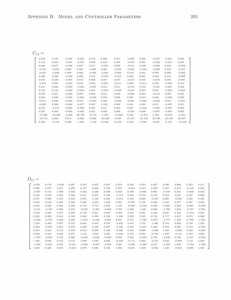
Appendix B. Model and Controller Parameters 203
C13 =
0.052 0.135 -0.000 -0.029 0.018 0.003 0.013 -0.000 0.085 -0.005 -0.001 0.025
0.112 0.204 -0.001 -0.027 0.039 0.019 0.037 -0.055 0.291 -0.046 -0.013 0.007
0.048 0.037 -0.000 0.007 0.017 -0.007 0.003 -0.014 0.039 -0.009 0.004 -0.002
-0.013 -0.056 0.000 0.004 -0.008 0.002 -0.003 -0.003 -0.004 -0.003 0.010 -0.015
-0.027 -0.048 0.000 0.009 -0.005 -0.002 -0.008 0.010 0.012 0.009 0.005 -0.002
0.020 0.039 -0.000 0.003 0.012 -0.016 -0.015 0.009 0.001 0.002 0.013 -0.009
0.019 0.030 -0.000 0.013 0.008 0.007 0.007 -0.013 0.045 -0.010 0.005 -0.005
-0.014 0.050 -0.000 0.010 0.004 -0.027 -0.011 0.004 -0.011 0.022 -0.004 0.014
0.041 0.022 -0.000 -0.003 -0.001 0.013 0.011 -0.015 0.103 -0.021 -0.001 0.002
0.110 0.110 -0.000 -0.004 0.035 -0.024 -0.008 -0.014 0.255 0.007 -0.002 -0.003
0.027 0.051 -0.000 0.009 0.004 0.014 0.002 -0.006 0.052 -0.012 0.006 0.001
0.024 0.029 -0.000 -0.004 -0.002 0.012 0.009 0.005 0.013 0.003 -0.008 0.006
-0.011 0.036 -0.000 0.010 -0.003 0.009 -0.008 -0.001 -0.004 -0.004 0.004 -0.001
-0.005 0.090 -0.000 -0.017 0.021 -0.021 0.003 0.001 0.003 0.011 -0.007 0.015
0.016 -0.019 -0.000 -0.002 0.001 0.011 0.005 0.001 -0.094 -0.006 -0.007 0.004
0.027 0.009 -0.000 -0.002 0.001 0.003 0.008 -0.003 0.026 -0.007 -0.005 0.002
-18.320 -25.966 -0.000 26.796 -2.712 -7.195 -12.892 0.942 -14.877 3.794 10.619 -5.950
-18.716 3.809 0.015 -2.260 -0.000 -23.600 -0.000 21.271 -21.558 25.786 -23.391 22.657
6.363 -6.134 0.008 -1.833 -1.189 10.439 10.335 0.346 -6.340 -6.867 -8.157 -13.332
D11 =
4.638 0.176 -0.049 0.067 0.347 0.837 0.487 0.370 0.565 0.553 0.507 0.596 0.686 0.224 0.411
0.369 3.377 0.221 0.269 0.177 0.266 0.529 0.761 -0.064 0.443 0.263 0.027 0.313 -0.149 0.355
-0.007 0.154 3.490 0.502 0.332 0.246 0.389 0.333 0.598 -0.085 0.861 -0.169 0.343 -0.069 0.034
0.228 0.278 0.508 3.384 0.411 0.277 0.136 -0.110 0.334 0.210 0.195 0.552 0.037 0.427 0.038
0.537 0.300 0.419 0.338 3.875 1.184 0.520 -0.014 0.162 0.626 -0.347 0.885 -0.005 1.245 0.491
0.643 0.148 0.243 0.124 0.845 4.033 1.032 0.561 -0.079 0.108 0.302 0.103 0.277 0.357 0.022
0.256 0.260 0.296 0.088 0.122 0.715 3.664 1.183 -0.480 -0.240 0.839 -0.684 0.690 -0.361 -0.088
-0.151 -0.165 0.390 0.105 -0.356 -0.305 -0.008 3.785 0.332 -1.281 2.208 -1.788 1.004 -0.757 -0.784
0.582 0.320 0.277 0.045 0.122 0.251 0.254 0.088 3.216 0.491 0.162 0.297 0.244 -0.143 0.387
0.982 0.362 0.454 0.120 0.386 0.493 0.126 -1.248 2.259 3.165 0.748 0.717 0.247 0.074 0.826
-0.342 -0.373 0.302 0.223 -0.433 -0.445 -0.087 0.441 0.751 -1.729 5.679 -1.777 1.239 -0.702 -1.083
1.359 0.492 0.207 0.195 0.663 0.833 0.270 -0.953 0.874 1.723 -1.085 5.764 0.026 0.758 1.265
0.269 -0.055 0.051 0.076 0.230 0.108 0.007 -0.120 0.401 -0.247 0.484 0.504 3.885 0.744 -0.565
0.474 0.342 0.155 0.135 0.913 0.609 0.186 -0.668 0.418 0.886 -1.068 1.440 -0.696 5.052 -0.003
0.588 0.323 0.228 0.251 1.134 1.006 0.401 -0.642 0.475 0.694 -0.760 1.185 -0.116 1.453 3.895
-1.379 -0.605 0.102 0.089 -0.858 -0.649 -0.208 0.609 0.246 -2.652 2.570 -2.838 0.789 -0.417 -3.506
1.496 0.939 0.197 0.135 1.390 1.846 0.962 -0.449 -0.112 2.660 -2.521 2.933 -0.993 1.118 2.846
-1.091 -0.641 0.042 -0.011 -0.992 -0.887 -0.059 1.691 -0.696 -2.399 2.917 -3.353 1.602 -1.734 -1.726
1.239 0.426 0.010 -0.025 0.379 0.586 0.129 1.692 -0.918 1.688 -0.934 1.120 -0.003 -0.088 1.335

Appendix B. Model and Controller Parameters 204
D12 =
-0.014 0.356 0.154 0.693
0.046 0.125 0.431 0.044
0.460 -0.320 0.476 -0.039
0.111 0.301 -0.181 0.272
-0.089 1.154 -0.368 0.658
1.003 0.199 0.824 -0.141
1.269 -1.120 1.682 -1.238
2.056 -2.680 1.763 -0.724
-0.372 0.402 0.060 0.594
-1.250 1.781 -1.317 1.602
2.514 -3.270 2.056 -1.522
-2.470 3.404 -2.236 2.210
1.340 -1.061 0.394 -0.289
-0.639 1.767 -1.452 1.349
-0.659 2.020 -1.114 1.029
8.838 -5.966 3.763 -2.909
-4.160 10.089 -3.146 3.104
4.427 -5.950 8.039 -3.645
-1.645 1.998 -0.408 4.525
B.3 Identified Model
The identified model (6.1) presented in section 6.1.2 is given by:
ΣSysID :
x(k + 1) = Ax(k) + Bu(k)
y(k) = Cx(k) + Du(k)(B.3)
The estimated system matrices A, B, C, D are as follows.
A =
0.672 -0.345 -0.063
0.636 -0.031 0.411
-0.012 -0.549 -0.606
B =
0.079
-0.137
-0.266
C =[
61.103 16.155 4.802]
D =[
0.000]

Appendix C
Control Circuitry
Figure C.1: Current amplification and protection circuit. The diagram shows the circuit
for four channels only. The circuit can be replicated to any desired number of channels.
205

Appendix C. Control Circuitry 206
Figure C.2: Response of the protection circuit. Note that the output voltage is limited
within ±1.5V .

Appendix D
Modal Reconstruction of the
Wavefront Shape
The wavefront slope data provided by the SHWS is used to reconstruct the wavefront
shape. Any appropriate set of 2D basis functions may be used for the reconstruction
purpose. A standard reconstruction algorithm using Zernike mode shapes is described in
the following.
Assume that for any wavefront profile ζ(x, y) measured by the SHWS, the wavefront
slope readings are available at K lenslets sub-apertures. The wavefront slope readings
can be assembled into a vector s ∈ R2K as:
s =[s1x, s1y
, s2x, s2y
, ..., skx, sky
, ..., sKx, sKy
]T(D.1)
where(skx, sky
)is the local average slope of the wavefront, ζ(x, y), at the kth lenslet,
and can be computed as follows:
skx=
∫∫
k
∂ζ(x,y)∂x
dxdy
∫∫
k
dxdy=
∆xskf
; sky=
∫∫
k
∂ζ(x,y)∂y
dxdy
∫∫
k
dxdy=
∆yskf
(D.2)
Here f is the focal length of the lenslet and, ∆xsk and ∆ysk are the displacement of the
sensor focal spots in the horizontal and vertical directions, respectively, from the center
of the lenslet k.
For any number J of Zernike modes specified for the reconstruction of the wavefront
207
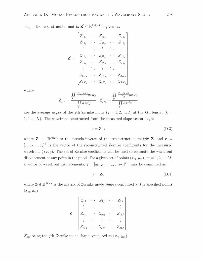
Appendix D. Modal Reconstruction of the Wavefront Shape 208
shape, the reconstruction matrix Z′ ∈ R
2M×J is given as:
Z′
=
Z11x· · · Zj1x
· · · ZJ1x
Z11y· · · Zj1y
· · · ZJ1y
.... . .
.... . .
...
Z1kx· · · Zjkx
· · · ZJkx
Z1ky· · · Zjky
· · · ZJky
.... . .
.... . .
...
Z1Kx· · · ZjKx
· · · ZJKx
Z1Ky· · · ZjKy
· · · ZJKy
where
Zjkx=
∫∫
k
∂Zj(x,y)
∂xdxdy
∫∫
k
dxdy; Zjky
=
∫∫
k
∂Zj(x,y)
∂ydxdy
∫∫
k
dxdy
are the average slopes of the jth Zernike mode (j = 1, 2, ..., J) at the kth lenslet (k =
1, 2, ..., K). The wavefront constructed from the measured slope vector, s , is
c = Z†s (D.3)
where Z† ∈ RJ×2K is the pseudo-inverse of the reconstruction matrix Z
′
and c =
[c1, c2, ..., cJ ]T is the vector of the reconstructed Zernike coefficients for the measured
wavefront ζ (x, y). The set of Zernike coefficients can be used to estimate the wavefront
displacement at any point in the pupil. For a given set of points (xm, ym) , m = 1, 2, ...,M ,
a vector of wavefront displacements, y = [y1, y2, ..., ym, ..yM ]T , may be computed as:
y = Zc (D.4)
where Z ∈ RM×J is the matrix of Zernike mode shapes computed at the specified points
(xm, ym)
Z =
Z11 · · · Z1j · · · Z1J
.... . .
.... . .
...
Zm1 · · · Zmj · · · ZmJ...
. . ....
. . ....
ZM1 · · · ZMj · · · ZMJ
Zmj being the jth Zernike mode shape computed at (xm, ym).