Turk J Elec Eng & Comp Sci

(2017) 25: 4223 – 4241

c⃝ TUBITAK

doi:10.3906/elk-1612-277

Turkish Journal of Electrical Engineering & Computer Sciences

http :// journa l s . tub i tak .gov . t r/e lektr ik/

Research Article

Modeling and control of a permanent-magnet brushless DC motor drive using a

fractional order proportional-integral-derivative controller

Swapnil KHUBALKAR1,∗, Anjali JUNGHARE1, Mohan AWARE1, Shantanu DAS2

1Department of Electrical Engineering, Visvesvaraya National Institute of Technology, Nagpur, India2Reactor Control System Design Section, E & I Group, Bhabha Atomic Research Centre, Mumbai, India

Received: 23.12.2016 • Accepted/Published Online: 28.05.2017 • Final Version: 05.10.2017

Abstract: This paper deals with the speed control of a permanent-magnet brushless direct current (PMBLDC) motor.

A fractional order PID (FOPID) controller is used in place of the conventional PID controller. The FOPID controller

is a generalized form of the PID controller in which the order of integration and differentiation is any real number. It

is shown that the proposed controller provides a powerful framework to control the PMBLDC motor. Parameters of

the controller are found by using a novel dynamic particle swarm optimization (dPSO) method. The frequency domain

pole-zero (p-z) interlacing method is used to approximate the fractional order operator. A three-phase inverter with four

switches is used in place of the conventional six-switches inverter to suggest a cost-effective control scheme. The digital

controller has been implemented using a field programmable gate array (FPGA). The control scheme is verified using

the FPGA-in-the-loop (FIL) wizard of MATLAB/Simulink. Improvement in the overall performance of the system is

observed using the proposed FOPID controller. The energy efficient nature of the FOPID controller is also demonstrated.

Key words: Fractional PID, particle swarm optimization, brushless DC, FPGA, tuning

1. Introduction

DC motors are widely used because the methods to control their speed are very simple and precise [1]. To

overcome the issue of mechanical wear out of DC motors, PMBLDC motors are being used [2]. Various

areas of application of PMBLDC motors are aerospace, domestic appliances, automotive, consumer, medical,

industrial automation, instrumentation, electric vehicles, etc. [3]. A few advantages of PMBLDC motors over

the conventional brushed DC motors include better speed-torque characteristics, higher efficiency, long operating

life, higher speed, noise-free operation, and lower maintenance. The torque to weight ratio of a PMBLDC motor

is also higher as compared to conventional DC motors [4].

PID controllers have been widely used in industry for many decades to improve the transient as well

as steady-state characteristics of the system in general [5]. The properties of fractional order operators (sα ,

where - 2 < α < 2) were explored in recent research work to enhance system performance [6–9]. The FOPID

controller is an extension of the traditional PID controller by using the theory of fractional calculus [10]. It

has five independent parameters, i.e. three controller gains (Kp , Ki , Kd ) and two additional fractional order

operators (α , β ). This expansion adds more robustness and flexibility to the system [7–9]. The advantages of

FOPID controllers over the integer order PID controllers include reduced steady-state error, reduced oscillations

∗Correspondence: swapnilkhubalkar@students.vnit.ac.in

4223

KHUBALKAR et al./Turk J Elec Eng & Comp Sci

and overshoot, reduced control efforts, better response time, robustness to variation in the gain of the plant

(iso-damping property), good output disturbance rejection, and inherent memory characteristics [6–12]. FOPID

controllers are tested in a few places like level control of a spherical tank, speed control of brushed DC and

permanent magnet DC motor, position control of Maglev systems, or chaotic system control [7–14].

Several tuning methods are available for FOPID controllers in both the time and frequency domains

[15]. Artificial intelligence (AI) tuning methods such as the artificial bee colony (ABC) algorithm, ant colony

optimization (ACO) algorithm, genetic algorithm (GA), bacterial swarm optimization (BSO), and particle

swarm optimization (PSO) are employed to find out the controller parameters [15–18]. The optimization

methods explore the multidimensional search space by using numerous particles, chromosomes, honey bees, or

bacteria. In a global search space issue, the AI optimization techniques perform superiorly compared to the

conventional techniques because of the randomness of the search, multiple solutions, more search space area

coverage, etc. [17]. From the AI point of view, the PSO technique is one of the most fruitful methods of

swarm intelligence [18]. This technique has several advantages like stable convergence characteristics, simple

implementation, and good computational efficiency. The dynamic weight concept is introduced in the PSO

method and a new algorithm is developed, which is known as dPSO [19]. The tuning method concentrates on

the minimization of the time domain-based objective function. The p-z interlacing approximation method is

used to realize fractional order operators in the sense of integer order [7, 20].

This paper aims to present a novel control scheme with a digitally implementable FOPID for a PMBLDC

motor drive. The approximation, tuning, and implementation of the FOPID controller are shown in the paper.

Improvement in transient and steady-state performance is supported by the results. A comparison with a

conventional PID controller and its analysis is provided to prove the effectiveness of the control scheme. The

major objectives of this paper include:

• Modeling and design of the digital FOPID-based PMBLDC motor drive.

• Suggestion of a cost-effective solution using a four-switch three-phase inverter in place of the conventional

six-switch inverter.

• Use of a frequency domain pole-zero interlacing algorithm to realize the FOPID controller and its imple-

mentation using an FPGA.

• Optimization of the FOPID controller through the dynamic PSO (dPSO) technique and its contribution

towards the improvement of the controller.

• Minimization of settling time, error signal, control signal, and phase currents by using the proposed

controller.

The rest of the paper is organized in the following way: Section 2 discusses the modeling of the PMBLDC

motor drive system, followed by the proposed controller design in Section 3. Section 4 discusses the control

scheme. Results are given in Section 5 and the paper is summarized in Section 6.

2. Modeling of the PMBLDC motor drive

Typical waveforms of a PMBLDC motor with square wave shaped phase current and trapezoidal back-emf

(electromotive force) distribution are shown in Figure 1 [4]. It is observed from Figure 1 that the back-emf

is fixed for 120 and changes linearly with the rotor angle before and after it. The phase currents and the

4224

KHUBALKAR et al./Turk J Elec Eng & Comp Sci

corresponding phase back-emf voltages need to be synchronized to drive the motor with constant maximum

torque [21]. In every mode, two phases are conducting while the other phase is silent.

2.1. Modeling of PMBLDC motor

Figure 2 displays the block diagram of a PMBLDC motor-fed four-switch three-phase inverter. The model of

the PMBLDC motor consists of three phases. The sum of three phase currents must add up to zero as in Eq.

(1).

Figure 1. Back emf waveforms.

Ia + Ib + Ic = 0 (1)

Here, Ia , Ib , Ic are the phase currents. The PMBLDC motor is presented by using a set of differential equations

as in Eq. (2).

Van = RaIa +d

dtλa + ean; Vbn = RbIb +

d

dtλb + ebn; Vcn = RcIc +

d

dtλc + ecn (2)

Here, Van , Vbn , Vcn are the phase voltages; Ra , Rb , Rc are the resistances of motor windings per phase; ean ,

ebn , ecn are phase to neutral back-emfs; and λa , λb , λc are the flux linkages. The PMBLDC motor model can

also be written as in Eq. (3). Van

Vbn

Vcn

=

Ra 0 00 Rb 00 0 Rc

IaIbIc

+d

dt[

La Lba Lca

Lab Lb Lcb

Lac Lbc Lc

IaIbIc

] + ea

ebec

(3)

As the permanent magnet is inducing the rotor field, it requires that the inductances should not be

4225

KHUBALKAR et al./Turk J Elec Eng & Comp Sci

dependent upon the rotor position, so:

La = Lb = Lc = Ls (4)

Lab = Lba = Lbc = Lcb = Lca = Lac = M (5)

Here, Ls is the self-inductance per phase and M is the mutual inductance per phase. Using Eqs. (4) and (5),

Eq. (3) reduces to:

Van

Vbn

Vcn

=

Ra 0 00 Rb 00 0 Rc

IaIbIc

+

Ls −M 0 00 Ls −M 00 0 Ls −M

d

dt

IaIbIc

+

eaebec

(6)

The flux linkages are represented as in Eq. (7).

λa = LsIa −M(Ib + Ic); λb = LsIb −M(Ia + Ic); λc = LsIc −M(Ib + Ia) (7)

Back-emf is the function of a rotor position (θr ) with amplitude of E = Kb ωm , where Kb is the

back-emf constant and ωm is the mechanical speed of the rotor. Back-emf of phase a is given in Eq. (8) and

similarly eb and ec can be written using Figure 1.

ea =

(6E/π)θr

E−(6E/π)θr + 6E

−E(6E/π)θr − 12E)

.....

0 < θr < π/6π/6 < θr < π/2π/2 < θr < 7π/67π/6 < θr < 3π/23π/2 < θr < 2π

(8)

The three phase currents are obtained by reorganizing Eq. (2) as:

dIadt

=1

Ls −M(Van − ea −RIa);

dIbdt

=1

Ls −M(Vbn − eb −RIb);

dIcdt

=1

Ls −M(Vcn − ec −RIc)

(9)

The electromagnetic torque (Te ) is obtained from Eq. (10):

Te =Zp

2ωr(eaIa + ebIb + ecIc) (10)

Here, Zp is the number of pole-pairs. The speed of the motor (ωr ) is obtained using the following differential

equation (Eq. (11)):

Te = TL + Jdωr

dt+Bωr (11)

4226

KHUBALKAR et al./Turk J Elec Eng & Comp Sci

Here, TL is the load torque, B is the frictional coefficient, and J is the moment of inertia. Rotor position in

electrical degrees is calculated using Eq. (12):

θr =

∫ωr.dt+ θ0 (12)

Here, θ0 is the rotor’s initial position. All these equations (Eqs. (1)–(12)) are used for modeling the PMBLDC

motor. The motor specifications are given in the Appendix.

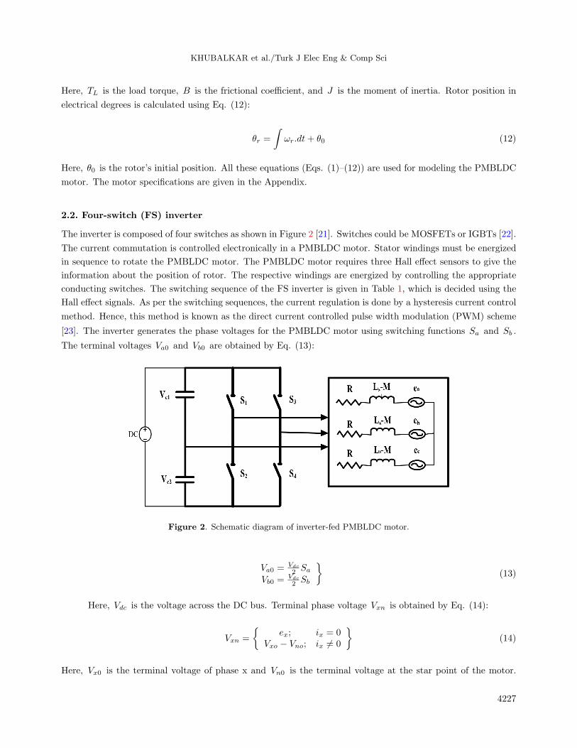
2.2. Four-switch (FS) inverter

The inverter is composed of four switches as shown in Figure 2 [21]. Switches could be MOSFETs or IGBTs [22].

The current commutation is controlled electronically in a PMBLDC motor. Stator windings must be energized

in sequence to rotate the PMBLDC motor. The PMBLDC motor requires three Hall effect sensors to give the

information about the position of rotor. The respective windings are energized by controlling the appropriate

conducting switches. The switching sequence of the FS inverter is given in Table 1, which is decided using the

Hall effect signals. As per the switching sequences, the current regulation is done by a hysteresis current control

method. Hence, this method is known as the direct current controlled pulse width modulation (PWM) scheme

[23]. The inverter generates the phase voltages for the PMBLDC motor using switching functions Sa and Sb .

The terminal voltages Va0 and Vb0 are obtained by Eq. (13):

Figure 2. Schematic diagram of inverter-fed PMBLDC motor.

Va0 = Vdc

2 Sa

Vb0 = Vdc

2 Sb

(13)

Here, Vdc is the voltage across the DC bus. Terminal phase voltage Vxn is obtained by Eq. (14):

Vxn =

ex;

Vxo − Vno;ix = 0ix = 0

(14)

Here, Vx0 is the terminal voltage of phase x and Vn0 is the terminal voltage at the star point of the motor.

4227

KHUBALKAR et al./Turk J Elec Eng & Comp Sci

Table 1. Switching sequence of FS inverter.

Mode Switches Active phases Silent phase

1 S4 BC A

2 S1, S4 AB C

3 S1 AC B

4 S3 BC A

5 S2, S3 AB C

6 S2 AC B

The voltage Vn0 in each mode is given by Eq. (15).

Vn0 =

(Vb0 − (eb + ec))/2;(Va0 + Vb0 − (ea + eb + ec))/3;

(Va0 − (ea + ec))/2;

Mode = 1, 4Mode = 2, 5Mode = 3, 6

(15)

Eqs. (13)–(15) are used to model the proposed four-switch inverter.

3. Design of the proposed FOPID controller

The FOPID controller has widened the control span from point to plane [10]. This can control real-world

processes more accurately with smaller control efforts [7, 9, 12]. A fractional order system can be represented

by the following differential equation (Eq. (16)).

aDαnf(t) + aD

αn−1f(t) + .... = Dβnf(t) +Dβn−1f(t) + .... (16)

Here, Dαn is the fractional derivative of order αn with respect to variable t . The FOPID controller is

shown by the differential equation in Eq. (17).

c(t) = Kpe(t) +KiD−αe(t) +KdD

βe(t) (17)

Here, c(t) is the control signal and e(t) is the error signal. Using Laplace transform, the controller’s

transfer function is expressed by Eq. (18).

c(s) = Kp +Kis−α +Kds

β , (α, β > 0) (18)

Here, Kp , Ki , Kd are the proportional, integral, and derivative constants and α, β are positive real

numbers. The fractional operator is of infinite order in the sense of integers. There is a need to approximate it

into a finite dimensional system [7,24–26]. The frequency domain p-z interlacing approximation method is used

to approximate the fractional operator, which is explained further.

3.1. Digital approximation of fractional-order operator with p-z interlacing algorithm

Each transfer function can be represented by its p-z pairs [7, 10]. The Bode magnitude plot of the noninteger

order transfer function possesses the slope of ± 20α dB/dec while the phase plot is constant at a value equal to

4228

KHUBALKAR et al./Turk J Elec Eng & Comp Sci

± 90α . This slope and phase angle can be obtained by interlacing real p-z pairs on a negative real axis. The

nth order approximation can be achieved within the desired band of frequency (ωL, ωH), as per the error band

(ε) around required phase angle ϕreq = 90α [20]. The algorithm is used to obtain the p-z pairs, which assures

the phase angle within the tolerance limit of approximately 1 . The p-z pairs are obtained in the algorithm as

follows in Eq. (19):

I pole, p1 = 10[ϕreq + 45 logωL

45 +1]

I zero, z1 = 10 ωL

II pole, p2 = 10[log(p1) + 2 − µ]

II zero, z2 = 10[log(z1) + 2 − µ]

until pn ≥ ωH

(19)

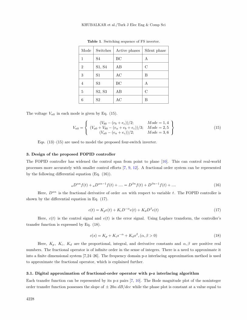
The asymptotic Bode phase plot of the fractional differentiator is shown in Figure 3 with α = 0.6, ϕreq =

54, ωL = 0.1 rad/s , and ωH = 1000 rad/s . For the given parameters, the actual phase plot oscillates with the

root mean squared (RMS) error of 0.001 (< 1). The average phase angle is obtained as 54.004 ≈ 54 , which

is approximately the same as ϕreq . Similarly, a fractional order integrator is designed.

−6 −4 −2 0 2 4 6 8−100

−80

−60

−40

−20

0

20

40

60

80

100

log10

ω →

Ph

ase

(deg

.)

→

Desired Band ofFrequency

Overall Exact plotZero

1

Pole1

Figure 3. Asymptotic phase plot with p-z pairs.

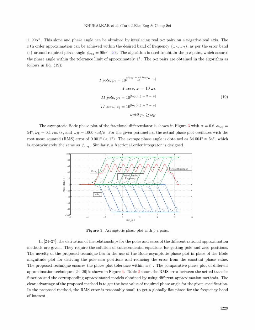
In [24–27], the derivation of the relationships for the poles and zeros of the different rational approximation

methods are given. They require the solution of transcendental equations for getting pole and zero positions.

The novelty of the proposed technique lies in the use of the Bode asymptotic phase plot in place of the Bode

magnitude plot for deriving the pole-zero positions and reducing the error from the constant phase value.

The proposed technique ensures the phase plot tolerance within ±ε . The comparative phase plot of different

approximation techniques [24–26] is shown in Figure 4. Table 2 shows the RMS error between the actual transfer

function and the corresponding approximated models obtained by using different approximation methods. The

clear advantage of the proposed method is to get the best value of required phase angle for the given specification.

In the proposed method, the RMS error is reasonably small to get a globally flat phase for the frequency band

of interest.

4229

KHUBALKAR et al./Turk J Elec Eng & Comp Sci

10−4

10−2

100

102

104

106

0

30

60

Ph

ase

(deg

)

Frequency (rad/s)

CRONE

Carlson’s method

Oustaloup’s method

Proposed method (p−z)

Required

Desired Band of Frequency

Figure 4. Comparative Bode phase plot for s0.6 .

Table 2. Comparison among [24–26] and proposed method for α = 0.6, ϕreq = 54 .

Algorithm Average value RMS error

CRONE [24] 47.653 17.7783

Carlson’s method [25] 40.598 11.1127

Oustaloup’s method [26] 53.281 4.8678

Proposed method 54.004 0.001

The digital FOPID controller is used so that its hardware implementation will be easy. The discretization

of the fractional operator sα is the key point of the digital implementation of the FOPID controller [28]. Two

steps are needed for discretization. The first one is the frequency domain approximation of the operator in

continuous time and the second one is discretizing the obtained continuous-time transfer function. Here, the

Tustin method is chosen for discretization with 0.001 s as sample time (T). Tustin approximation uses the

formula given in Eq. (20).

z = esT ≈ 1 + sT/2

1− sT/2(20)

The discretization c(z) of continuous time transfer function c(s) is obtained as:

c(z) = c(s′), where s′ =2

T

z − 1

z + 1(21)

4230

KHUBALKAR et al./Turk J Elec Eng & Comp Sci

3.2. Tuning methodology: the dPSO method

In this paper, the controller parameters are obtained by using the dynamic particle swarm optimization method.

Every particle in the moving swarm presents a solution of the problem, which is determined by velocity as well

as position [18]. The position vector of every particle is denoted by the unknown parameters to be found. The

required number of particles is called the population. Every particle in the population travels with updated

direction and velocity to come nearer to the required solution. The dPSO algorithm is a modification of the

conventional PSO method. The product of difference in the objective function value between a particle and

its global best or individual best is added in dPSO. The change in a particle’s position is in direct proportion

with the iteration, which relies upon the global best, individual best, and a random velocity [19]. The dPSO

algorithm analyzes the workspace with the velocity of a particle, which is obtained as in Eq. (22):

vid = (f(pid)− f(xid))× (pid − xid)× sf1 + (f(pgd)− f(xid))× (pgd − xid)× sf2+

rand()× randn()× sf3(22)

Here, pid is the individual best, pgd is the global best, xid is the current position of the particle, vid is

the velocity of the particle, rand is a random function, randn is a random positive/negative value generator,

and sf1, sf2, sf3 are scaling factors. The size of the population is considered to be 200, maximum iterations

are set as 100, and the desired band of frequencies is selected as ωL = 0.1 rad/s , ωH = 1000 rad/s . Integrated

time absolute error (ITAE) is selected as an objective function to be minimized because of good selectivity. The

change in the system’s parameters influences the value of the ITAE, which gives a significant improvement in

parameter tuning [18, 29]. The ITAE function is given in Eq. (23):

JITAE =

∫ ∞

0

t|e(t)|dt (23)

Here, e(t) gives the deviation between the actual value and specified value. The objective function

value JITAE is reduced from 0.5398 (with PID) to 0.4051 (with FOPID), which denotes an improvement of

performance of about 24.95%. The values of the controller parameters obtained in Table 3 are used in the PID

and FOPID controllers.

Table 3. dPSO optimized controller parameters.

S. N. ControllerGain and fractional order value

Kp Ki Kd λ µ

1. PID 8 1.295 0.22 1 1

2. FOPID 4.25 0.2 0.099 1.21 0.6

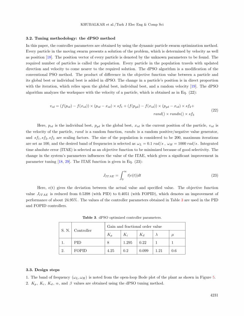
3.3. Design steps

1. The band of frequency (ωL, ωH) is noted from the open-loop Bode plot of the plant as shown in Figure 5.

2. Kp , Ki , Kd , α , and β values are obtained using the dPSO tuning method.

4231

KHUBALKAR et al./Turk J Elec Eng & Comp Sci

Frequency (rad/s)

−60

−40

−20

0

20

40

System: PMBLDCPeak gain (dB): 29.7At frequency (rad/s): 118

Mag

nit

ud

e (d

B)

101

102

103

104

−180

−135

−90

−45

0

System: PMBLDCPhase Margin (deg): 7.74Delay Margin (sec): 0.000269At frequency (rad/s): 503Closed loop stable? Yes

Ph

ase

(deg

)

PMBLDC

Figure 5. Open-loop Bode plot of PMBLDC motor.

3. The controller transfer function is computed using Eq. (18).

4. Eq. (18) is approximated using the p-z interlacing method and then discretized.

c(z) =

116.4z17 − 773.7z16 + 1797z15 − 802.6z14 − 3730z13 + 6455z12 − 1002z11−6953z10 + 6347z9 + 914z8 − 4282z7 + 1860z6 + 606.9z5−

730.9z4 + 162.1z3 + 29.75z2 − 15.32z + 1.248

z17 − 5.487z16 + 8.358z15 + 7.378z14 − 33.62z13 + 20.23z12 + 35.87z11−51.52z10 − 2.157z9 + 40.67z8 − 18.39z7 − 11.29z6 + 10.83z5−

0.4359z4 − 1.979z3 + 0.481z2 + 0.09213z − 0.03333

(24)

5. The approximated controller transfer function as in Eq. (24) is used in the control scheme as a speed

controller and the performance of the PMBLDC motor is observed.

4. Control scheme

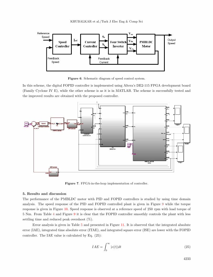
Figure 6 presents a schematic diagram of the speed control scheme of a PMBLDC motor. A four-switch inverter-

fed PMBLDC motor drive with a novel digital FOPID controller is modeled as discussed in Sections 2 and 3.

PID and FOPID controllers are considered to control the speed of the motor drive in this control scheme. A

reference speed is given as input and the controller provides the control signal in accordance with the generated

speed error. The generated reference current is fed as input to the current controller. Further, the current

controller generates switching pulses, which are generated by comparing the reference input signal and modes

generated from the motor module to operate the switches of an inverter. The simulation is carried out in the

MATLAB environment.

4.1. FPGA-in-the-loop implementation

The control scheme is verified using the FPGA-in-the-loop (FIL) wizard of MATLAB/Simulink. The FPGA-in-

loop implementation of the control scheme is given in Figure 7. Figure 8 shows the FIL implementation windows.

4232

KHUBALKAR et al./Turk J Elec Eng & Comp Sci

Figure 6. Schematic diagram of speed control system.

In this scheme, the digital FOPID controller is implemented using Altera’s DE2-115 FPGA development board

(Family Cyclone IV E), while the other scheme is as it is in MATLAB. The scheme is successfully tested and

the improved results are obtained with the proposed controller.

Figure 7. FPGA-in-the-loop implementation of controller.

5. Results and discussion

The performance of the PMBLDC motor with PID and FOPID controllers is studied by using time domain

analysis. The speed response of the PID and FOPID controlled plant is given in Figure 9 while the torque

response is given in Figure 10. Speed response is observed at a reference speed of 250 rpm with load torque of

5 Nm. From Table 4 and Figure 9 it is clear that the FOPID controller smoothly controls the plant with less

settling time and reduced peak overshoot (%).

Error analysis is given in Table 5 and presented in Figure 11. It is observed that the integrated absolute

error (IAE), integrated time absolute error (ITAE), and integrated square error (ISE) are lower with the FOPID

controller. The IAE value is calculated by Eq. (25):

IAE =

∫ ∞

0

|e(t)|dt (25)

4233

KHUBALKAR et al./Turk J Elec Eng & Comp Sci

Figure 8. FPGA-in-the-loop windows.

0 0.1 0.2 0.3 0.4 0.5 0.6 0.7 0.8 0.9 10

50

100

150

200

250

300

Time (s)

Spee

d (

rpm

)

with FOPID

with PID

Desired set speed

Figure 9. Speed response of the PID- and FOPID-controlled plant.

Table 4. Performance analysis.

S. N. Controller Overshoot (%) Settling time (s)

1.PID 1.6 0.35

FOPID 0.8 0.065

The ITAE value is calculated by Eq. (26):

ITAE =

∫ ∞

0

t|e(t)|dt (26)

4234

KHUBALKAR et al./Turk J Elec Eng & Comp Sci

0 0.05 0.1 0.15 0.2 0.25 0.3 0.35 0.4 0.45 0.5−40

−20

0

20

40

60

80

Time (s)

To

rqu

e (N

m)

for FOPID

for PID

Figure 10. Torque response of the PID- and FOPID-controlled plant.

Figure 11. Error signal analysis of PID- and FOPID-controlled plant.

Table 5. Error and control signal analysis.

S.N. ControllerError signal Control signal

ITAE IAE ISE ITACE IACE ISCE

1 PID 3.047 25.53 3154 239.1 817.7 994,000

2 FOPID 1.145 9.568 1300 5.934 43.1 24,350

The ISE value is calculated by Eq. (27):

ISE =

∫ ∞

0

|e(t)|2dt (27)

The error is related to an integral part of the controller. In the integral path, as the error moves over time, the

integral will continue to sum it up and multiply it by constant Ki . The integral path is used to remove constant

error in the system; no matter how small the error, it will sum up that error, which will be significant enough

to adjust the controller output. With FOPID, not only the integrator gain but also the integration order is

adjustable. Hence, it effectively controls the speed as compared to its integer counterpart.

4235

KHUBALKAR et al./Turk J Elec Eng & Comp Sci

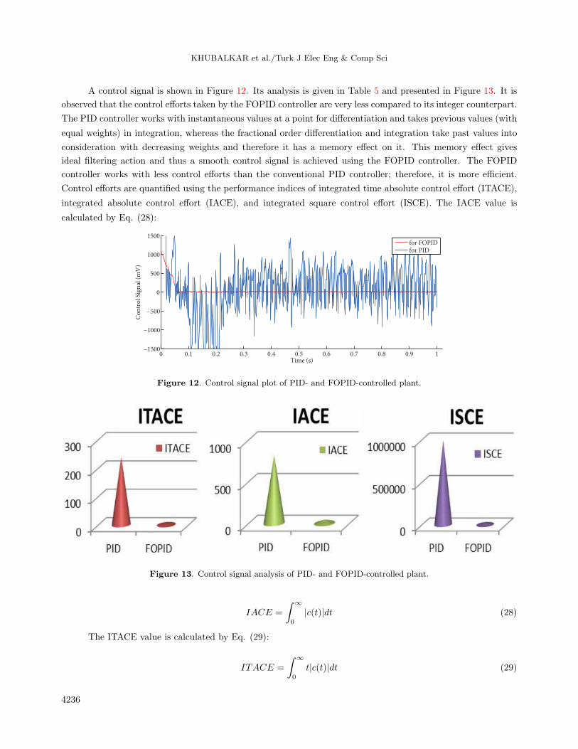
A control signal is shown in Figure 12. Its analysis is given in Table 5 and presented in Figure 13. It is

observed that the control efforts taken by the FOPID controller are very less compared to its integer counterpart.

The PID controller works with instantaneous values at a point for differentiation and takes previous values (with

equal weights) in integration, whereas the fractional order differentiation and integration take past values into

consideration with decreasing weights and therefore it has a memory effect on it. This memory effect gives

ideal filtering action and thus a smooth control signal is achieved using the FOPID controller. The FOPID

controller works with less control efforts than the conventional PID controller; therefore, it is more efficient.

Control efforts are quantified using the performance indices of integrated time absolute control effort (ITACE),

integrated absolute control effort (IACE), and integrated square control effort (ISCE). The IACE value is

calculated by Eq. (28):

0 0.1 0.2 0.3 0.4 0.5 0.6 0.7 0.8 0.9 1−1500

−1000

−500

0

500

1000

1500

Time (s)

Co

ntr

ol

Sign

al (

mV

)

for FOPIDfor PID

Figure 12. Control signal plot of PID- and FOPID-controlled plant.

Figure 13. Control signal analysis of PID- and FOPID-controlled plant.

IACE =

∫ ∞

0

|c(t)|dt (28)

The ITACE value is calculated by Eq. (29):

ITACE =

∫ ∞

0

t|c(t)|dt (29)

4236

KHUBALKAR et al./Turk J Elec Eng & Comp Sci

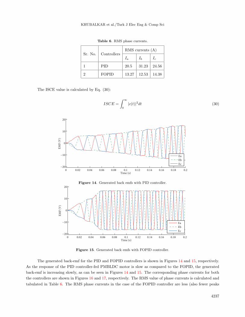
Table 6. RMS phase currents.

Sr. No. ControllersRMS currents (A)

Ia Ib Ic

1 PID 20.5 31.23 24.56

2 FOPID 13.27 12.53 14.38

The ISCE value is calculated by Eq. (30):

ISCE =

∫ ∞

0

|c(t)|2dt (30)

0 0.02 0.04 0.06 0.08 0.1 0.12 0.14 0.16 0.18 0.2−20

−10

0

10

20

Time (s)

EM

F (

V)

Ea

Eb

Ec

Figure 14. Generated back emfs with PID controller.

0 0.02 0.04 0.06 0.08 0.1 0.12 0.14 0.16 0.18 0.2−20

−10

0

10

20

Time (s)

EM

F (

V)

Ea

Eb

Ec

Figure 15. Generated back emfs with FOPID controller.

The generated back-emf for the PID and FOPID controllers is shown in Figures 14 and 15, respectively.

As the response of the PID controller-fed PMBLDC motor is slow as compared to the FOPID, the generated

back-emf is increasing slowly, as can be seen in Figures 14 and 15. The corresponding phase currents for both

the controllers are shown in Figures 16 and 17, respectively. The RMS value of phase currents is calculated and

tabulated in Table 6. The RMS phase currents in the case of the FOPID controller are less (also fewer peaks

4237

KHUBALKAR et al./Turk J Elec Eng & Comp Sci

are observed in the current waveforms), which suggests that the proposed scheme with the FOPID controller is

energy-efficient. The modes generated for controlling the inverter switches are given in Figure 18.

0 0.05 0.1 0.15 0.2 0.25 0.3−6

−4

−2

0

2

4

6

Time (s)

Cu

rren

t (A

)

Ia

a)Phasecurrent‘ I a ’

0 0.05 0.1 0.15 0.2 0.25 0.3−6

−4

−2

0

2

4

6

Time (s)

Cu

rren

t (A

)

Ib

b)Phasecurrent‘ Ib’

0 0.05 0.1 0.15 0.2 0.25 0.3−6

−4

−2

0

2

4

6

Time (s)

Cu

rren

t (A

)

Ic

c)Phasecurrent‘ I c’

Figure 16. Phase currents with PID controller.

6. Conclusion

The speed control of a fractional order PID-controlled PMBLDC motor is investigated to provide a solution

for implementing the high-performance motor drive. A closed-loop controlled PMBLDC drive is modeled and

4238

KHUBALKAR et al./Turk J Elec Eng & Comp Sci

0 0.05 0.1 0.15 0.2 0.25 0.3−6

−4

−2

0

2

4

6

Time (s)

Cu

rren

t (A

)

Ia

a)Phasecurrent‘ I a ’

0 0.05 0.1 0.15 0.2 0.25 0.3−6

−4

−2

0

2

4

6

Time (s)

Cu

rren

t (A

)

Ib

b)Phasecurrent‘ Ib’

0 0.05 0.1 0.15 0.2 0.25 0.3−6

−4

−2

0

2

4

6

Time (s)

Cu

rren

t (A

)

Ic

c)Phasecurrent‘ I c’

Figure 17. Phase currents with FOPID controller.

0 0.02 0.04 0.06 0.08 0.1 0.12 0.14 0.16 0.18 0.21

2

3

4

5

6

Time (s)

Mo

de

Mode

Figure 18. Mode generated to select switches.

4239

KHUBALKAR et al./Turk J Elec Eng & Comp Sci

simulated using MATLAB/Simulink. The model is tested in FPGA-in-the-loop and the results are presented.

The results of the conventional PID and FOPID controller-fed PMBLDC motor are compared. It is seen that

the proposed FOPID controller reduces overshoot, rise time, settling time, IAE, ISE, and ITAE in comparison

with the conventional PID controller. Control efforts of the proposed controller are also much less. The current

required to drive the motor is less, which points towards the energy-efficient nature of FOPID controllers. In

reference to the analysis, it can be summarized that the best-tuned FOPID can perform better than the best-

tuned PID. The digital controller is implemented using FPGA and tested in the FPGA-in-the loop wizard.

To get results that are even more promising it would be better to design the controller using multiobjective

optimization techniques.

Acknowledgment

The work presented in this paper was supported by the BRNS (Board of Research in Nuclear Sciences), India.

Sanction No. 2012 / 36 / 69.

References

[1] Hughes A, Drury B. Electric Motors and Drives: Fundamentals, Types and Applications. Waltham, MA, USA:

Newnes, 2013.

[2] Aydogdu O, Akkaya R. An effective real coded GA based fuzzy controller for speed control of a BLDC motor

without speed sensor. Turk J Electr Eng Co 2011; 19: 413-430.

[3] Pillay P, Krishnan R. Modeling, simulation and analysis of permanent magnet motor drives, part II: The brushless

DC motor drive. IEEE T Ind Appl 1989; 25: 274-279.

[4] Krishnan R. Permanent-Magnet Synchronous and Brushless DC Motor Drives. Boca Raton, FL, USA: CRC Press,

2009.

[5] Astrom K, Hagglund T. The future of PID control. Control Eng Pract 2001; 9: 1163-1175.

[6] Ranjbaran K, Tabatabaei M. Fractional order [PI], [PD] and [PI][PD] controller design using Bode’s integrals. Int

J Dynam Control (in press).

[7] Das S. Functional Fractional Calculus. 2nd ed. New York, NY, USA: Springer, 2011.

[8] Aware MV, Junghare AS, Khubalkar SW, Dhabale A, Das S, Dive R. Design of new practical phase shaping circuit

using optimal polezero interlacing algorithm for fractional order PID controller. Analog Integr Circ S 2017; 91:

131-145.

[9] Chopade AS, Khubalkar SW, Junghare AS, Aware MV, Das S. Design and implementation of digital fractional

order PID controller using optimal pole-zero approximation method for magnetic levitation system. IEEE/CAA J

Automatica Sinica 2016; 99: 1-12.

[10] Podlubny I. Fractional order systems and PIλDµ -controllers. IEEE T Automat Contr 1999; 44: 208-214.

[11] Shah P, Agashe S. Review of fractional PID controller. Mechatronics 2016; 38: 29-41.

[12] Khubalkar S, Chopade A, Junghare A, Aware M, Das S. Design and realization of stand alone digital fractional

order PID controller for buck converter fed DC motor. Circ Syst Signal Pr 2016; 35: 2189-2211.

[13] Atan O, Chen D, Turk M. Fractional order PID and application of its circuit model. J Chin Inst Eng 2016; 39:

695-703.

[14] Celik V, Demir Y. Effects on the chaotic system of fractional order PIα controller. Nonlinear Dynam 2010; 59:

143-159.

[15] Das S, Saha S, Das S, Gupta A. On the selection of tuning methodology of FO-PID controllers for the control of

higher order processes. ISA T 2011; 50: 376-388.

4240

KHUBALKAR et al./Turk J Elec Eng & Comp Sci

[16] Ozdemir MT, Ozturk D, Eke I, Celik V, Lee KY. Tuning of optimal classical and fractional order PID parameters

for automatic generation control based on the bacterial swarm optimization. IFAC-PapersOnline 2015; 48: 501-506.

[17] Jin Y, Branke J. Evolutionary optimization in uncertain environments: a survey. IEEE T Evolut Comput 2005; 9:

303-317.

[18] Maiti D, Acharya A, Chakraborty M, Konar A, Janarthanan R. Tuning PID and PI?D? controllers using the integral

time absolute error criterion. In: Proceedings of the 4th International Conference on Information and Automation

for Sustainability; December 2008; Colombo, Sri Lanka. New York, NY, USA: IEEE. pp. 457462.

[19] Badar AQH, Umre BS, Junghare AS. Reactive power control using dynamic particle swarm optimization for real

power loss minimization. Int J Elec Power 2012; 41: 133-136.

[20] Dhabale AS, Dive R, Aware MV, Das S. A new method for getting rational approximation for fractional-order

differintegrals. Asian J Control 2015; 17: 2143-2152.

[21] Lee BK, Kim TH, Ehsani M. On the feasibility of four-switch three phase BLDC motor drives for low cost commercial

applications- topology and control. IEEE T Power Electr 2003; 18: 164-172.

[22] Sathyan A, Milivojevic N, Lee YJ, Krishnamurthy M, Emadi A. An FPGA based novel digital PWM control scheme

for BLDC motor drives. IEEE T Ind Electron 2009; 56: 3040-3049.

[23] Rodriguez F, Emadi A. A novel digital control technique for brushless DC motor drives. IEEE T Ind Electron 2007;

54: 2365-2373.

[24] Carlson G, Halijak C. Approximation of fractional capacitors (1/s)1/n by a regular Newton process. IEEE T Circuit

Theory 1964; 11: 210-213.

[25] Oustaloup A. La commande CRONE: commande robuste d’ordre non entier. Paris, France: Hermes, 1991 (in

French).

[26] Oustaloup A, Levron F, Mathieu B, Nanot F. Frequency-band complex noninteger differentiator: characterization

and synthesis. IEEE T Circuits I 2000; 47: 25-39.

[27] de Oliveira Valerio DPM. Ninteger v. 2.3 Fractional Control Toolbox for MatLab. User and Programmer Manual.

Lisbon, Portugal: University of Lisbon, 2005.

[28] Machado JT. Discrete-time fractional order controllers. Fractional Calculus and Applied Analysis 2001; 4: 47-66.

[29] Zheng W, Pi Y. Study of the fractional-order proportional integral controller for the permanent magnet synchronous

motor based on the differential evolution algorithm. ISA T 2016; 63: 387-393.

4241

KHUBALKAR et al./Turk J Elec Eng & Comp Sci

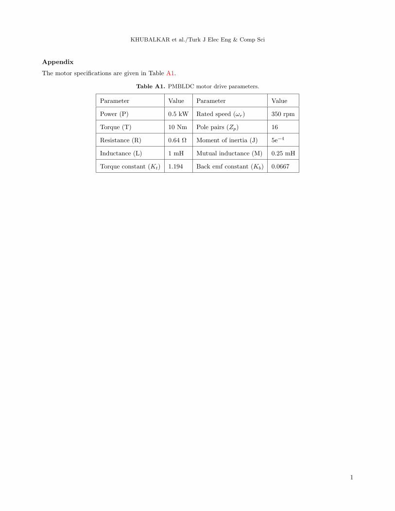
Appendix

The motor specifications are given in Table A1.

Table A1. PMBLDC motor drive parameters.

Parameter Value Parameter Value

Power (P) 0.5 kW Rated speed (ωr) 350 rpm

Torque (T) 10 Nm Pole pairs (Zp) 16

Resistance (R) 0.64 Ω Moment of inertia (J) 5e−4

Inductance (L) 1 mH Mutual inductance (M) 0.25 mH

Torque constant (Kt) 1.194 Back emf constant (Kb) 0.0667

1