International Journal on Electrical Engineering and Informatics - Volume 10, Number 4, Desember 2018

Modeling and Fuzzy Command Approach to Stabilize

the Wind Generator

Nejib Hamrouni and Sami Younsi

Analysis and treatment of energetic and electric systems (ATEES)

Science Faculty of Tunis-University of Tunis El Manar

hamrouni_nejib2003@yahoo.fr

Abstract: In this paper, a problem of mechanical modeling and robustly stabilization of a

wind system formed by a turbine, a driving shaft and an induction machine, is considered.

To overcome the complexity and the non-linearity of the system, the model of the wind

generator is approximated by a Takagi-Sugeno fuzzy model. Hence, to stabilize the obtained

fuzzy model, two command approaches were developed. They are the fuzzy controller using

the parallel distributed compensation (PDC) and the 𝐻∞ controller based-fuzzy observer.

Numerical optimization problems using linear matrix inequality (LMI) and convex

techniques are used to analyze the stability of the wind generator. Finally, simulation

examples illustrating the control performance and dynamic behavior of the wind generator

under various command approaches are presented.

Keywords: wind generator; modeling; H∞ command; LMI approach; stability;

1. Introduction

In recent decades, wind energies were well developed and exploited. They became

competitive thanks to the evolution of the power electronics. Nevertheless, the optimal

exploitation of the renewable energy sources encountered many problems which are related

mainly to the uncertain variation of the wind speed. To resolve these problems and to improve

the penetration rate and the stability level of the connected wind system, several controls are

developed focusing this subject. These commands illustrate performance limits such as

instability and implementation complexity.

Recently many studies have been devoted to the stability of the nonlinear system. Fuzzy

control constitutes a preferment command which has attracted an increasing attention because it

can offer an effective solution to the control of complex, uncertain and undefined system [1-3].

The well-known Takagi-Sugeno (TS) fuzzy method has become a convenient approach for

dealing with a complex system. This approach provides an effective representation of the system

with the aid of fuzzy sets, fuzzy rules and a local linear model. The Takagi Sugeno fuzzy model

[4] constitutes a productive way to describe and control the dynamics of nonlinear systems [5].

The TS fuzzy dynamics model is a system described by the fuzzy ‘if-then’ rules which offer

local linear representation. The advantages of using this approach for design control are that the

closed loop stability analysis using Lyapunov method becomes easier to apply and the controller

synthesis can be reduced to convex problem [6]. Once the nonlinear models are transferred to a

fuzzy model, control design can be carried out. Some of them are fuzzy controller using parallel

distribution compensation (PDC) and the fuzzy observer-based H∞ controller. The PDC approach

employs multiple linear controllers corresponding to the locally linear plants [7]. Many

applications illustrate the effectiveness of the TS models and parallel distribution compensation

[4, 8]. Fuzzy observer-based H∞ controller has been developed in [9, 10]. Stability and aptitude

to reject exterior disturbances provided by this command approach were approved in [11].

In this work, the TS-fuzzy approach is used to approximate the nonlinear wind generator

model. Two approaches of robust and powerful commands to stabilize the mechanical part of the

wind generator are presented. In the first part, a fuzzy controller design uses the concept of PDC

[7, 12] is studied. In the second part, a fuzzy observer-based H∞ controller is developed in order

Received: August 20th, 2016. Accepted: Desember 25th, 2018

DOI: 10.15676/ijeei.2018.10.4.3

648

to improve the performance of the system and to minimize the disturbance effect of the wind

speed. Sufficient stability conditions are expressed in terms of LMI which can be solved very

efficiently using convex optimization techniques [6]. Finally, simulation examples are given to

illustrate both stability and robustness analysis of the proposed control systems.

2. Description and modeling of the wind generator

The drive train of the wind turbine generator system consists of the following elements: a

blade-pitching mechanism, a hub with blades, a rotor shaft, a gearbox and generator. The

common way to model the drive train is to treat the system as a number of discrete masses

connected together by springs defined by damping and stiffness coefficients (Figureure 1).

Figure 1. Transmission model of 6 masses connected together

The aerodynamic part is made of three blades, hub, gearbox and generator. This system has

six inertias; three blade inertias (Jp1, Jp2 and Jp3), hub inertia Ja, gearbox inertia Jm (Jm1, Jm2) and

generator inertia Jg. The elasticity between adjacent masses is expressed by Kp1, Kp2, Kp3, Ka and

Kg. The mutual damping between adjacent masses is given by fp1, fp2, fp3, Da and dg. There exist

torque losses through external damping elements represented by αp1, αp2 and αp3. θp1, θp2, θp3, θa,

θm and θg represent respectively angular positions of the blades, the hub, the gearbox and the

generator. Ωp1, Ωp2, Ωp3, Ωa, Ωm (Ωm1, Ωm2) and Ωg are respectively the angular velocities of the

blades, hub, gearbox and generator. Fp1, Fp2 and Fp3 are aerodynamic torques acting on each

blade. The sum of the blade torques constitutes the turbine torque Ct. Cm (Cm1, Cm2) and Cg are

respectively the gearbox and generator torques. It is assumed that the aerodynamic torque acting

on the hub is zero.

Figure 2. Three-mass model

fp1

fp2

fp3

Kp1

Kp2

Kp3

αp1

αp2

αp3

Fp1

Fp2

Fp3

Ka

Da

(Ja)

(θa)

(Ωa)

Kg

dg

Dg

Cg Jg, Ωg, θg

(Cm2, Jm2, θm2, Ωm2)

(Cm1, Jm1, θm1, Ωm1) (Ct)

Jp1, θp1

Jp2, θp2

Jp3, θp3

Blades Hub Gearbox Generator

Fp Ka

Da

(Ja)

(θa)

(Ωa)

Kg

dg

Dg

Cg Jg, Ωg, θg

(Cm2, Jm2, θm2, Ωm2)

(Cm1, Jm1, θm1, Ωm1) (Ct)

Nejib Hamrouni, et al.

649

In order to simplify the control of the wind generator, we introduce some simplifications on

the six masse models. The turbine inertia can be calculated from the combined weight of the

blades and the hub. Therefore, the mutual damping and elasticity between the hub and the three

blades is ignored (Kp1= Kp2=Kp3≈0 and fp1= fp2= fp3≈0). The torque losses of the blades (αp1, αp2

and αp3) are ignored because turbine speed is very weak. Moreover, it is assumed that the three

blades have uniform weight distribution (Fp1=Fp2=Fp3=Fp) and the turbine torque is assumed to

be equal to the sum of the torque acting on the various blades. Thus, the turbine can be looked

as a large disk with small thickness and the wind system (three blades, hub, gearbox and

generator) can be modeled by three masses coupled through a gearbox as indicated by Figure. 2.

In addition, compared with the mechanical characteristics of the blades and the generator,

the gearbox inertia and mutual damping with adjacent masses moment of inertia are ignored.

Therefore, the complex system can be simplified to be two-mass model through reforming the

dynamic system with the equivalent stiffness and damping coefficients. As a consequence, the

two-mass model contains two parts which represent the wind turbine and the generator. They are

connected by a flexible shaft. This model will be used to investigate the control of the wind

turbine.

Figure 3. Two-mass model

Referring to the simplified diagram given by Figure.3 and the Newton’s second law for

rotational masses, the dynamic system can be formulated with respect to the wind turbine rotor

and the electromagnetic generator [13].

𝑗𝑡𝑡 + 𝐷𝑡(Ω𝑡 − Ω𝑔) + 𝐾ℎ(𝜃𝑡 − 𝜃𝑔) = 𝐶𝑎𝑒𝑟

𝑗𝑔𝑔 + 𝐷𝑡(Ω𝑔 − Ω𝑡) + 𝐾ℎ(𝜃𝑔 − 𝜃𝑡) = −𝐶𝑔

(1)

With

• Jt, Jg: turbine and generator inertias [kgm²].

• Caer, Cg: aerodynamic and electromagnetic torques of the turbine and generator [Nm].

• Ωt, Ωg: angular speed of the turbine and generator [rd/s].

• θt, θg: angular displacement of the turbine and generator [rd].

• Kh: elasticity between the turbine and the generator [Nm/rd].

• Dt: damping between the turbine and the generator [Nms/rd].

According to eq.1, the model of the conversion system is written as:

𝑑(Ω𝑡)

𝑑𝑡=

𝐾ℎ

𝑗𝑡𝜃𝑠 −

𝐷𝑡

𝑗𝑡(Ω𝑡 − Ω𝑔) +

𝐶𝑎𝑒𝑟

𝑗𝑡𝑑(Ω𝑔)

𝑑𝑡=

𝐾ℎ

𝑗𝑔𝜃𝑠 +

𝐷𝑡

𝑗𝑔(Ω𝑡 − Ω𝑔) −

𝐶𝑔

𝑗𝑔

(2)

Fp Kh

Dt

Jt, θt, Ωt, Ct

Dg

Cg Jg, Ωg, θg

Modeling and Fuzzy Command Approach to Stabilize

650

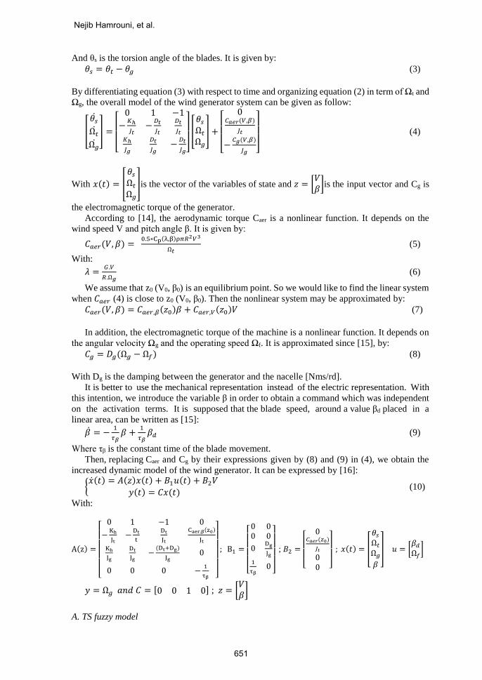
And θs is the torsion angle of the blades. It is given by:

𝜃𝑠 = 𝜃𝑡 − 𝜃𝑔 (3)

By differentiating equation (3) with respect to time and organizing equation (2) in term of Ωt and

Ωg, the overall model of the wind generator system can be given as follow:

[

𝜃Ω𝑡

Ω

] =

[ 0 1 −1

−𝐾ℎ

𝐽𝑡−𝐷𝑡

𝐽𝑡

𝐷𝑡

𝐽𝑡𝐾ℎ

𝐽𝑔

𝐷𝑡

𝐽𝑔−𝐷𝑡

𝐽𝑔]

[

𝜃𝑠Ω𝑡Ω𝑔

] +

[

0𝐶𝑎𝑒𝑟(𝑉,𝛽)

𝐽𝑡

−𝐶𝑔(𝑉,𝛽)

𝐽𝑔 ]

(4)

With 𝑥(𝑡) = [

𝜃𝑠Ω𝑡Ω𝑔

]is the vector of the variables of state and 𝑧 = [𝑉𝛽]is the input vector and Cg is

the electromagnetic torque of the generator.

According to [14], the aerodynamic torque Caer is a nonlinear function. It depends on the

wind speed V and pitch angle β. It is given by:

𝐶𝑎𝑒𝑟(𝑉, 𝛽) = 0.5∗Cp(λ,β)ρ𝜋𝑅

2𝑉3

Ω𝑡 (5)

With:

𝜆 =𝐺.𝑉

𝑅.Ω𝑔 (6)

We assume that z0 (V0, β0) is an equilibrium point. So we would like to find the linear system

when 𝐶𝑎𝑒𝑟 (4) is close to z0 (V0, β0). Then the nonlinear system may be approximated by:

𝐶𝑎𝑒𝑟(𝑉, 𝛽) = 𝐶𝑎𝑒𝑟,𝛽(𝑧0)𝛽 + 𝐶𝑎𝑒𝑟,𝑉(𝑧0)𝑉 (7)

In addition, the electromagnetic torque of the machine is a nonlinear function. It depends on

the angular velocity Ωg and the operating speed Ωf. It is approximated since [15], by:

𝐶𝑔 = 𝐷𝑔(Ω𝑔 − Ω𝑓) (8)

With Dg is the damping between the generator and the nacelle [Nms/rd].

It is better to use the mechanical representation instead of the electric representation. With

this intention, we introduce the variable β in order to obtain a command which was independent

on the activation terms. It is supposed that the blade speed, around a value βd placed in a

linear area, can be written as [15]:

= −1

𝜏𝛽𝛽 +

1

𝜏𝛽𝛽𝑑 (9)

Where τβ is the constant time of the blade movement.

Then, replacing Caer and Cg by their expressions given by (8) and (9) in (4), we obtain the

increased dynamic model of the wind generator. It can be expressed by [16]:

(𝑡) = 𝐴(𝑧)𝑥(𝑡) + 𝐵1𝑢(𝑡) + 𝐵2𝑉

𝑦(𝑡) = 𝐶𝑥(𝑡) (10)

With:

A(z) =

[ 0 1 −1 0

−Kh

Jt−Dt

t

Dt

Jt

Caer,β(z0)

JtKh

Jg

Dt

Jg−(Dt+Dg)

Jg0

0 0 0 −1

τβ ]

; B1 =

[ 0 00 0

0Dg

Jg1

τβ0]

; 𝐵2 =

[

0𝐶𝑎𝑒𝑟(𝑧0)

𝐽𝑡

00 ]

; 𝑥(𝑡) = [

𝜃𝑠Ω𝑡Ω𝑔𝛽

] 𝑢 = [𝛽𝑑Ω𝑓]

𝑦 = Ω𝑔 𝑎𝑛𝑑 𝐶 = [0 0 1 0] ; 𝑧 = [𝑉𝛽]

A. TS fuzzy model

Nejib Hamrouni, et al.

651

The objective of this approach is to approximate the nonlinear system by linearized sub-

systems. It has been used as an alternative to classical models to capture dynamic performances

under different operating conditions and in different functioning zones.

The description of the nonlinear system in terms of “If-Then” rules combined with a

mathematical description of nonlinear systems is called a Takagi-Sugeno fuzzy model. The

concept of sector nonlinearity provided means for exact approximation of nonlinear systems by

fuzzy blending of set locally linearized sub-systems. The TS system is defined as follows:

If 𝑧1(𝑡) is 𝐹𝑖1 and… and 𝑧𝑝(𝑡) is 𝐹𝑖𝑝 then [17]:

= 𝐴𝑖𝑥(𝑡) + 𝐵𝑖𝑢(𝑡)

𝑦(𝑡) = 𝐶𝑖𝑥(𝑡) i=1,2…M] (11)

Where 𝑥(𝑡) ∈ ℜ𝑛 is the state vector, M is the number of rules “If-Then”, 𝐹𝑖𝑗 represent the

corresponding fuzzy set. They are the degree of membership of zi(t), 𝑖 = 1, … , 𝑝, 𝑢(𝑡) ∈ ℜ

𝑚is the control input vector, 𝑦(𝑡) ∈ ℜ𝑞is the output vector. 𝐴𝑖 ∈ ℜ

𝑛∗𝑚, 𝐶𝑖 ∈ ℜ𝑞∗𝑛 and

𝐵𝑖 ∈ ℜ𝑛∗𝑚 are system matrices of appropriates dimension. 𝑧1(𝑡)…𝑧𝑝(𝑡) are nonlinear

functions of the state variables. They are called as premise variables.

The inferred system states are governed by:

(𝑡) =∑ 𝑤𝑖(𝑧(𝑡))(𝐴𝑖𝑥(𝑡)+𝐵𝑖𝑢(𝑡))𝑀𝑖=1

∑ 𝑤𝑖(𝑧(𝑡))𝑀𝑖=1

= ∑ 𝜇𝑖(𝑧(𝑡))(𝐴𝑖𝑥(𝑡) + 𝐵𝑖𝑢(𝑡))𝑀𝑖=1 (12)

Where:

𝜇𝑖(𝑧(𝑡)) =𝑤𝑖(𝑧(𝑡))

∑ 𝑤𝑖(𝑧(𝑡))𝑀𝑖=1

, 𝑤𝑖(𝑧(𝑡)) = ∏ 𝐹𝑖𝑗(𝑧𝑗(𝑡))𝑝𝑗=1 and 𝑤𝑖(𝑧(𝑡)) ≥ 0 When t ≥ 0.

The output signal is obtained by the same technique:

𝑦(𝑡) = ∑ 𝜇𝑖(𝑧(𝑡))𝐶𝑖𝑥(𝑡)𝑀𝑖=1 (13)

The term 𝜇𝑖(𝑧(𝑡))determines the activation terms of the associated local models. According

to the functioning zone of the system, these terms indicate the contribution of the local model.

They allow a progressive passage of a local model to another and they depend on the state vector.

They can be in triangular or Gaussian forms. They satisfy the conditions given in [17].

∑ 𝜇𝑖(𝑥(𝑡)) = 1 𝑀𝑖=1

0 < 𝜇𝑖(𝑥(𝑡)) ≤ 1 (14)

B. TS fuzzy description of the wind generator

We consider the TS fuzzy models based on the nonlinear sectors [18-19] to represent the

nonlinear model of the wind system composed of a turbine, a driving shaft and an induction

machine. This approach based on the transformation of the scalar functions and the bornitude of

the continuous variables V and β. These variables are limited as given by the following equations.

𝑉𝑚𝑖𝑛 ≤ 𝑉 ≤ 𝑉𝑚𝑎𝑥 and 𝛽𝑚𝑖𝑛 ≤ 𝛽 ≤ 𝛽𝑚𝑎𝑥

According to the model given by the equation (10), the system has two non linearties

depending on V and β. To linearize this model, we will use the presentation

of TS previously presented. For those non-linearities, the base comprises four rules ‘If-Then’.

Thus, the nonlinear wind system is represented by the following fuzzy model:

𝐼𝑓 𝛽 𝑖𝑠 𝐹11 𝑎𝑛𝑑 𝑉 𝑖𝑠 𝐹2

1 𝑡ℎ𝑒𝑛 (𝑡) = 𝐴1𝑥(𝑡) + 𝐵1𝑢(𝑡) + 𝐵21 𝑤

𝑦 = 𝐶1𝑥(𝑡)

𝐼𝑓 𝛽 𝑖𝑠 𝐹11 𝑎𝑛𝑑 𝑉 𝑖𝑠 𝐹2

2 𝑡ℎ𝑒𝑛 (𝑡) = 𝐴2𝑥(𝑡) + 𝐵1𝑢(𝑡) + 𝐵22𝑤

𝑦 = 𝐶2𝑥(𝑡)

𝐼𝑓 𝛽 𝑖𝑠 𝐹12 𝑎𝑛𝑑 𝑉 𝑖𝑠 𝐹2

1 𝑡ℎ𝑒𝑛 (𝑡) = 𝐴3𝑥(𝑡) + 𝐵1𝑢(𝑡) + 𝐵23𝑤

𝑦 = 𝐶3𝑥(𝑡)

𝐼𝑓 𝛽 𝑖𝑠 𝐹12 𝑎𝑛𝑑 𝑉 𝑖𝑠 𝐹2

2 𝑡ℎ𝑒𝑛 (𝑡) = 𝐴4𝑥(𝑡) + 𝐵1𝑢(𝑡) + 𝐵24𝑤

𝑦 = 𝐶4𝑥(𝑡)

Then the inferred system is given by:

Modeling and Fuzzy Command Approach to Stabilize

652

(𝑡) = ∑ 𝜇𝑖(𝑧(𝑡))((

4𝑖=1 𝐴𝑖𝑥(𝑡) + 𝐵1𝑢(𝑡) + 𝐵2𝑖𝑤))

𝑦 = ∑ 𝜇𝑖(𝑧(𝑡)4𝑖=1 𝐶𝑖𝑥(𝑡)

(15)

Where μi (z (t)) are activation terms of the subsystems. They are given by:

μ1(z) = F1

1(β)F21(V)

μ2(z) = F11(β)F2

2(V)

μ3(z) = F12(β)F2

1(V)

μ4(z) = F12(β)F2

2(V)

(16)

With 𝐹𝑖𝑗are the degrees of membership function of the activation terms. They are given by:

F1

1(β) =β−β1

β2−β1

F12(β) =

β2−β

β2−β1

F21(V) =

V−V1

V2−V1

F22(V) =

V2−V

V2−V1

(17)

With V1=Vmin, V2=Vmax, β1=βmin and β2=βmax.

For i = 1...4, the matrices 𝐴𝑖 𝐵1, 𝐵2𝑖 and C are given by:

𝐴1 = 𝐴2 =

[ 0 1 −1 0

−𝐾ℎ

𝐽𝑡−𝐷𝑡

𝐽𝑡

𝐷𝑡

𝐽𝑡

𝐶𝑎𝑒𝑟,𝛽1

𝐽𝑡

𝐾ℎ

𝐽𝑔

𝐷𝑡

𝐽𝑔−(𝐷𝑡+𝐷𝑔)

𝐽𝑔0

0 0 0 −1

𝜏𝛽 ]

;𝐴3 = 𝐴4 =

[ 0 1 −1 0

−𝐾ℎ

𝐽𝑡−𝐷𝑡

𝐽𝑡

𝐷𝑡

𝐽𝑡

𝐶𝑎𝑒𝑟,𝛽2

𝐽𝑡

𝐾ℎ

𝐽𝑔

𝐷𝑡

𝐽𝑔−(𝐷𝑡+𝐷𝑔)

𝐽𝑔0

0 0 0 −1

𝜏𝛽 ]

𝐵21 = 𝐵23 =

[ 0

𝐶𝑎𝑒𝑟,𝑉1

𝐽𝑡

00 ]

; 𝐵1 =

[ 0 00 0

0𝐷𝑔

𝐽𝑔

1

𝜏𝛽0]

; 𝐵22 = 𝐵24 =

[ 0

𝐶𝑎𝑒𝑟,𝑉2

𝐽𝑡

00 ]

; 𝐶 = [0 0 1 0]

With:

𝐶𝑎𝑒𝑟,𝛽1 = 𝐶𝑎𝑒𝑟,𝛽(𝛽 = 𝛽1) 𝐶𝑎𝑒𝑟,𝛽2 = 𝐶𝑎𝑒𝑟,𝛽(𝛽 = 𝛽2)

𝐶𝑎𝑒𝑟,𝑉2 = 𝐶𝑎𝑒𝑟,𝑉(𝑉 = 𝑉2) 𝐶𝑎𝑒𝑟,𝑉1 = 𝐶𝑎𝑒𝑟,𝑉(𝑉 = 𝑉1)

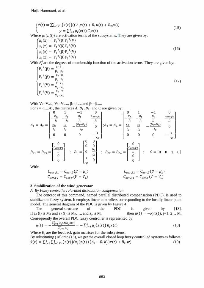
3. Stabilization of the wind generator

A. By Fuzzy controller: Parallel distribution compensation

The concept of this command, named parallel distributed compensation (PDC), is used to

stabilize the fuzzy system. It employs linear controllers corresponding to the locally linear plant

model. The general diagram of the PDC is given by Figure 4.

The general structure of the PDC is given by [18].

If z1 (t) is M1 and z2 (t) is M2…., and zp is Mp then 𝑢(𝑡) = −𝐾𝑗𝑥(𝑡), j=1, 2… M.

Consequently the overall PDC fuzzy controller is represented by:

𝑢(𝑡) = −∑ 𝑤𝑗(𝑧)𝐾𝑗𝑥(𝑡)4𝑗=1

∑ 𝑤𝑗4𝑗=1

= −∑ 𝜇𝑗(𝑧(𝑡))4𝑗=1 𝐾𝑗𝑥(𝑡) (18)

Where Kj are the feedback gain matrices for the subsystems.

By substituting (18) into (15), we get the overall closed loop fuzzy controlled systems as follows:

(𝑡) = ∑ ∑ 𝜇𝑖(𝑧(𝑡))(𝜇𝑗(𝑧(𝑡))4𝑗=1

4𝑖=1 (𝐴𝑖 − 𝐵1𝐾𝑗)𝑥(𝑡) + 𝐵2𝑖𝑤) (19)

Nejib Hamrouni, et al.

653

Figure 4. General diagram of parallel distributed compensation

Table 1. Parameters of the wind system

Symbol quantity value

Kh Elasticity of driving shaft 1.566×106Nm-1

Dr Damping factor shaft-nacelle 3029.5Nmsrad-1

Dg Damping factor IG-gearbox 15.993Nmsrad-1

Jg Inertia of IG 5.9 kgm²

Jp Inertia of blades 830000kgm²

ρ Air density 1.225kgm-3

R Blade radius 30.3m

τβ Time constant of the blade movement 100ms

P Rated power of the IG 1MW

p Pole pair number of the IG 3

λopt Optimal specific speed 7

Cpmax Coefficient of maximal power 0.48

γ Desired level disturbance attenuation 0.6

Caer,β1 Aerodynamic torque corresponding to the pitch angle β1 723980Nm

Caer,β2 Aerodynamic torque corresponding to the pitch angle β2 376070Nm

Caer,v1 Aerodynamic torque corresponding to the wind speed V1 106440Nm

Caer,v2 Aerodynamic torque corresponding to the wind speed V2 85370Nm

The fuzzy controller design consists in determining the local feedback gain Kj ( j=1, 2, 3, 4)

for the corresponding parts of TS models so that the zero equilibrium of the closed loop fuzzy

systems was globally stable. We apply the quadratic stability theorem of the global system, yields

the following results [9]: the equilibrium of the closed loop system (19) is globally stable, if there

is a common positive definite matrix P which satisfies the following conditions:

−𝑋𝐴𝑖

𝑇 − 𝐴𝑖𝑋 + 𝐵𝑖𝑀𝑖 + (𝐵𝑖𝑀𝑗)𝑇 > 0

−𝑋𝐴𝑖𝑇 − 𝐴𝑖𝑋 − 𝑋𝐴𝑗

𝑇 − 𝐴𝑗𝑋 +𝑀𝑗𝑇𝐵𝑖

𝑇 + 𝐵𝑖𝑀𝑗 +𝑀𝑖𝑇𝐵𝑗

𝑇 + 𝐵𝑗𝑀𝑖 ≥ 0 (20)

The objective of the command is in finding K1, K2, K3 and K4 and P>0 that satisfy the

conditions presented by equation 20. An approach to design a stable fuzzy controller for the wind

generator is to transform the condition in eq. 20 into convex problem [1, 21-23]. The solution of

the stable PDC controller design problem via linear matrix inequalities (LMI) for the system

leads to:

𝐾𝑗 = 𝑀𝑗𝑋−1 with 𝑃 = 𝑋−1 (21)

If the solution of the LMI (eq. 20) is found, it means that local state feedback gains Kj (j=1,

2, 3 and 4) provide quadratic stability of the closed loop TS fuzzy systems. Hence, using matlab

toolbox, the controller parameters are found to be:

Multi-models

or

TS model

TS fuzzy control :

𝑢(𝑡) = −𝜇𝑗(𝑧(𝑡))

4

𝑗=1

𝐾𝑗𝑥(𝑡)

u(t)

x(t)

y(t)

Disturbance: Wind

Modeling and Fuzzy Command Approach to Stabilize

654

𝐾1 = [−4225 −1645 2225 −208

−1 108 −107 77 104 −992 102]

𝐾2 = [−4225 −1645 2225 −208

−1 108 −1.05 107 77 104 −992 102]

𝐾3 = [−4225,5 −1644,85 2265 −208,35

−1,08 108 −1.05 107 77,04 104 −992,1 102] 𝐾4

= [−4225,45 −1644,82 2265 −208,32

−1,065 108 −1.05 107 77,05 104 −992,1 102]

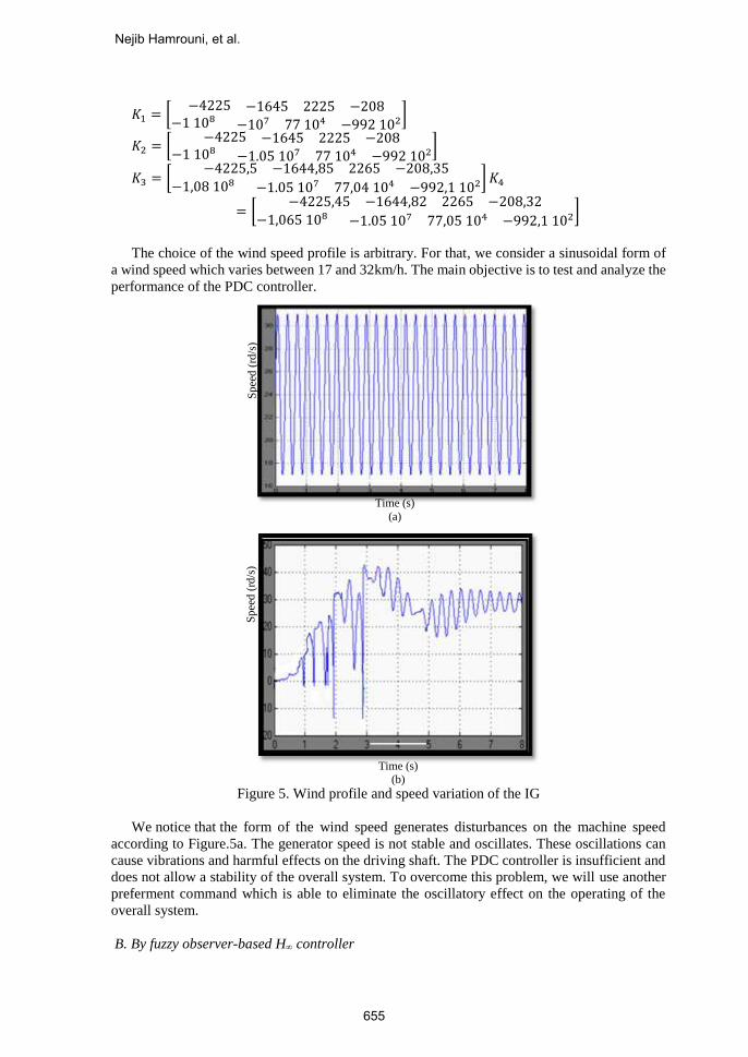
The choice of the wind speed profile is arbitrary. For that, we consider a sinusoidal form of

a wind speed which varies between 17 and 32km/h. The main objective is to test and analyze the

performance of the PDC controller.

Figure 5. Wind profile and speed variation of the IG

We notice that the form of the wind speed generates disturbances on the machine speed

according to Figure.5a. The generator speed is not stable and oscillates. These oscillations can

cause vibrations and harmful effects on the driving shaft. The PDC controller is insufficient and

does not allow a stability of the overall system. To overcome this problem, we will use another

preferment command which is able to eliminate the oscillatory effect on the operating of the

overall system.

B. By fuzzy observer-based H∞ controller

Sp

eed

(rd

/s)

Sp

eed

(rd

/s)

Time (s)

(a)

Time (s)

(b)

Nejib Hamrouni, et al.

655

The approach is to develop a robust command which permits to obtain robustness stability in

analytical way. According to the TS system represented by eq.12, some state variables aren’t

measured. Hence, it was obligatory to synthesize an observer which make possible to estimate

those variables (θs and β). The design of fuzzy observer obliges that the local models of the

system should be locally observables, and is obtained by interpolation of several Luenberger

observer. The observer is introduced as follows:

If 1(𝑡)is Fi1 and…p(𝑡)is Fip, then for i=1 …4, the observer states are governed by [24]:

(𝑡) = 𝐴𝑖(𝑡) + 𝐵1𝑢(𝑡) + 𝐵2𝑖𝑤(𝑡) − 𝐿𝑖(𝑦(𝑡) − (𝑡))

(𝑡) = 𝐶𝑖(𝑡) (22)

Where Li is the observer gain for the ith observer rule. The overall fuzzy observer is represented

as follows:

(𝑡) = ∑ 𝜇𝑖((𝑡)) (𝐴𝑖(𝑡) + 𝐵1𝑢(𝑡) + 𝐵2𝑖𝑤(𝑡) − 𝐿𝑖(𝑦(𝑡) − (𝑡)))

4𝑖=1

(𝑡) = ∑ 𝜇𝑖((𝑡))4𝑖=1 𝐶𝑖(𝑡)

(23)

Where (𝑡)𝜖 ℜ𝑛and (𝑡)𝜖 ℜℎ are respectively the estimated state and output vector.

The stabilization of the generator speed is essentially a disturbance rejection problem. Thus, a

robust control using H∞ technique is well adopted to resolve this kind of control problem. It is

assumed that the fuzzy systems are locally controllable. Hence, a fuzzy controller with the

following rules can be used.

If 1(𝑡)is Fi1 and…p(𝑡)is Fjp

Then 𝑢(𝑡) = 𝐾𝑗(𝑡), for j=1 to 4.

Hence, the fuzzy control is given by [9]:

𝑢(𝑡) = ∑ 𝜇𝑗((𝑡))𝐾𝑗(𝑡)4𝑗=1 (24)

Figure 6. General diagram of the H∞ command with fuzzy observer

With 𝐾𝑗 are the controller gains.

Let use a new variable which present the estimation error. It is given by:

𝑒(𝑡) = (𝑡) − 𝑥(𝑡) (25)

The closed loop fuzzy model of the wind system integrating the TS model (15), the fuzzy

observer (23) and the controller (24) became:

(x(t)

z(t)) = ∑ ∑ μj(z(t))μi(z(t))

4j=1

4i=1 (

Aij Bi

C 0) (x(t)

w(t)) (26)

With:

TS fuzzy model

Eq. (15)

Fuzzy H∞ control

𝑢(𝑡) =𝜇𝑗(𝑧(𝑡))

4

𝑗=1

𝐾𝑗(𝑡)

u(t)

x(t)

y(t)

Disturbance: Wind

TS fuzzy-observer

Eq. (23) (𝑡)

(𝑡)

Modeling and Fuzzy Command Approach to Stabilize

656

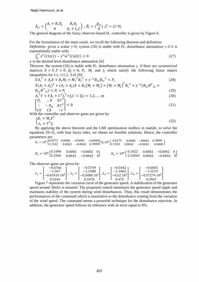
𝑖𝑗 = (𝐴𝑖 + 𝐵1𝐾𝑗 𝐵1𝐾𝑗

0 𝐴𝑖 + 𝐿𝑖𝐶) ; 𝑖 = (

𝐵2𝑖0) ;𝐶 = (𝐶 0)

The general diagram of the fuzzy observer-based H∞ controller is given by Figure 6.

For the formulation of the main result, we recall the following theorem and definition.

Definition: given a scalar γ>0, system (26) is stable with H∞ disturbance attenuation γ if it is

exponentially stable with:

∫ 𝑧𝑇(𝑡)𝑧(𝑡)∞

0− 𝛾2𝑤𝑇(𝑡)𝑑(𝑡) < 0 (27)

𝛾 is the desired level disturbance attenuation [6].

Theorem: the system (26) is stable with H∞ disturbance attenuation γ, if there are symmetrical

matrices 𝑋 > 0 ,𝑌 > 0 , 𝑄𝑖 > 0, 𝑃𝑖 , 𝑀𝑖 and 𝐽𝑖 which satisfy the following linear matrix

inequalities for i<j =1.2, 3.4 [6]:

𝑋𝐴𝑖𝑇 + 𝐴𝑖𝑋 + 𝐵1𝑀𝑖 +𝑀1

𝑇𝐵1𝑇 + 𝛾−2𝐵2𝑖𝐵2𝑖

𝑇 < 𝑃𝑖 (28)

𝑋(𝐴𝑖 + 𝐴𝑗)𝑇 + (𝐴𝑖 + 𝐴𝑗)𝑋 + 𝐵1(𝑀𝑖 +𝑀𝑗) + (𝑀𝑖 +𝑀𝑗)

𝑇𝐵1

𝑇 + 𝛾−2(𝐵2𝑖𝐵𝑇2𝑗 +

𝐵2𝑗𝐵𝑇2𝑖) < 𝑃𝑖 + 𝑃𝑗 (29)

𝐴𝑖𝑇𝑌 + 𝑌𝐴𝑖 + 𝐶

𝑇𝐽𝑖𝑇+𝐽𝑖𝐶 < 𝑄𝑖i = 1,2, … ,m (30)

[𝑃1 …0 𝑋𝐶𝑇

⋮ ⋱ 𝑃𝑚 𝑋𝐶𝑇

𝐶𝑋 𝐶𝑋 −𝐼

] < 0 (31)

With the controller and observer gains are given by:

𝐾𝑖 = 𝑀𝑖𝑋

𝑇

𝐿𝑖 = 𝑌𝑇𝐽𝑖

(32)

By applying the above theorem and the LMI optimization toolbox in matlab, to solve the

equations 29-32, with four fuzzy rules, we obtain set feasible solutions. Hence, the controller

parameters are:

𝐾1 = 106 [0.0273 0.0000 −0.0001 −0.00002.1542 0.0042 −0.0042 0. 0000

] 𝐾2106 [

0.0275 0.0000 −00001 0. 00002.1543 0.0042 −0.0042 0.0000

]

𝐾3 = 106 [0.1096 0.0002 −0.0002 02.1504 0.0042 −0.0042 0

] 𝐾4 = 106 [0.1022 0.0002 −0.0002 0 2.15043 0.0042 −0.0042 0

]

The observer gains are given by:

𝐿1 = [

−0.6766−1.367

−0.65416 103

0.5244

] ; 𝐿2 = [

−0.5749−1.1588

−0.5488 103

0.3478

] ;𝐿3 = [

−0.5442−1.1062−0.52 103

0.475

] ; 𝐿4 = [

−0.6043−1.2213

−0.57274 103

0.3947

]

Figure 7 represents the variation curve of the generator speed. A stabilization of the generator

speed around 30rd/s is ensured. The proposed control minimizes the generator speed ripple and

maintains stability of the system during wind disturbances. Thus, this result demonstrates the

performances of the command which is insensitive to the disturbance coming from the variation

of the wind speed. The command seems a powerful technique for the disturbance rejection. In

addition, the generator speed follows its reference with an error equal to 8%.

Nejib Hamrouni, et al.

657

Figure 7. Variation curve of the generator speed (measure and reference)

Figure 8. Variation of the state variables of the system: (a): torsion angle; (b): pitch angle

Sp

eed

s (r

d/s

)

Time (s)

Ωg

Ωgref

Time (s)

An

gle

(rd

)

(a)

Time (s)

An

gle

(rd

)

(b)

Modeling and Fuzzy Command Approach to Stabilize

658

Curve 8 represents the variation of the state variables of the TS fuzzy system. Figure.8a

represents the estimated and measure angle torsion of the driving shaft. Figure.8b

represents the variation of the pitch angle of the blades. The measured and estimated values are

confused justifying consequently the performances of fuzzy observer-based H∞ controller.

Stability results for closed model based H∞ controller have been achieved assuming that all of

the system states are measurable.

4. Conclusion

In this paper, an approach of modeling and control of a nonlinear system based-wind

generator is discussed. In the first part, a TS fuzzy model is used to approximate the dynamics

of wind generator composed of a turbine, a driving shaft and an induction machine. In the second

part, two command approaches are developed around the complex system in order to stabilize

the mechanical model and to minimize the generator speed ripple. Numerical optimization

problems using linear matrix inequality and convex techniques are used to design the controller

and the observer parameters.

Stability results for closed model based fuzzy controller using the concept of PDC have been

examined assuming that all of the system states are measurable. The generator speed curve shows

that the fuzzy controller can’t stabilize the response of system when the wind speed varies. The

proposed command scheme using fuzzy observer-based H∞ controller illustrates some good

performances. It minimizes the generator speed ripple, maintains stability of the system during

wind disturbances and permits the attenuation of the external disturbances. The obtained results

illustrate the effectiveness of this approach to stabilize the nonlinear system. Moreover, they

showed the ability of the command to reject the disturbances and make possible to obtain a stable

wind generator without oscillations. Therefore, we consider that the fuzzy observer-based H∞

controller is appropriate for the nonlinear system control with external disturbances.

5. Acknowledgment

The authors wish to thank the Ministry of High Education and Scientific Research for

providing subsidies within the framework of the young researcher projects.

6. References

[1]. S.G. Cao, N.W. Rees and G. Feng, “Analysis and design for a class of complex control

systems part II: fuzzy controller design,” Automatica, Vol. 33, pp. 1029–1039, 1997.

[2]. G. Feng, “A survey on analysis and design of model-based fuzzy control systems,” IEEE

Transactions on Fuzzy Systems, vol. 14, pp. 676-697, 2006.

[3]. G. Feng, “Analysis and Synthesis of Fuzzy Control Systems: A Model-Based Approach,”

in: CRC Press, New York, 2010.

[4]. T. Takagi and M. Sugeno, “Fuzzy identification of systems and its applications to modeling

and control,” IEEE Trans. Syst, vol. 15, pp. 116– 132, 1985.

[5]. S.G. Cao, N.W. Rees and G. Feng, “H∞ control of uncertain fuzzy continuous time

systems,” IEEE Transactions on Fuzzy Systems, vol. 8, pp. 171-190, 2000.

[6]. J. Park, J. Kim and D. Park, “LMI-based design of stabilizing fuzzy controllers for

nonlinear systems described by Takagi-Sugeno fuzzy model,” Fuzzy Sets Syst., vol. 122,

pp. 73-82, 2001.

[7]. S.K. Hong and R. Langari, “An LMI-based fuzzy control system design with TS

framework,” Infor. Sci., vol. 123, pp. 163-179, 2000.

[8]. K.R. Lee, E.T. Jeung and H.B Park, “Robust fuzzy H∞ control for uncertain nonlinear

systems via state feedback: an LMI approach,” International Journal of Fuzzy Sets and

Systems, vol. 120, pp.123–134, 2001.

[9]. K. Tanaka and H.O. Wang, Fuzzy control systems design and analysis: a linear matrix

inequality approach, Wiley, New York, 2001.

[10]. K. Tanaka and H.O Wang, “Fuzzy regulators and fuzzy observers: a linear matrix inequality

approach,” Proc. 36th IEEE Conf. on Decision and Control, vol. 6, pp. 1315–1320, 1997.

Nejib Hamrouni, et al.

659

[11]. [11] K. Tanaka, T. Ikeda and H.O. Wang, “Fuzzy regulators and fuzzy observers,” IEEE

Trans. Fuzzy Syst., vol. 6, pp. 250– 256, 1998.

[12]. E. Kamal, M. Koutb , A. A. Sobaih and B. Abozalam, “An Intelligent Maximum Power

Extraction Algorithm for Hybrid Wind-Diesel-Storage System", Int. J. Electr. Power

Energy Syst., vol. 32, pp. 170-177, 2010.

[13]. M. Santoso, “Dynamic Models for Wind Turbines and Wind Power Plants,” The University

of Texas at Austin, January 11, 2008.

[14]. R. Babouria, D. Aouzellagb and K. Ghedamsi, “Integration of Doubly Fed Induction

Generator Entirely Interfaced w ith Network in a Wind Energy Conversion System,”

Energy Procedia, vol. 36, pp. 169 – 178, 2013.

[15]. N. Hamrouni, A. Ghobber, A. Rabhi and A. E. Hajjaji, “Modeling and robust control of a

wind Generator,” International Conference on Electrical Sciences and Technologies in

Maghreb (CISTEM), Tunisia, 2014

[16]. F.D. Bianchi and R.J. Mantz, “Gain scheduling control of variable speed wind energy

conversion systems using quasi-LPV models,” Control Engineering Practice, vol. 13, pp.

247-255, 2005.

[17]. M. Oudghiri, M. Chadli and A. El Hajjaji, “One-Step Procedure for Robust Output H∞

Fuzzy Control,” The 15th IEEE Mediterranean Conference on control and Automation

MED’07, Athens, Greece, 2007.

[18]. H.O. Wang, K. Tanaka and M.F. Griffin, “An approach to fuzzy control of nonlinear

systems: stability and design issues,” IEEE Transactions on Fuzzy Systems, vol. 4, pp. 14-

23, 1996.

[19]. K. Tanaka, T. Ikeda and H.O. Wang, “Robust stabilization of a class of uncertain nonlinear

systems via fuzzy control: quadratic stabilizability, H∞ control theory, and linear matrix

inequalities,” IEEE Transactions on Fuzzy Systems, vol. 4, pp. 1-13, 1996.

[20]. E. Kamal, A. Aitouche, R. Ghorbani and M. Bayart, “Fuzzy Scheduler Fault-Tolerant

Control for Wind Energy Conversion Systems,” IEEE Transactions on Control Systems

Technology, vol. 22, pp. 119-131, 2013.

[21]. S.K. Song and R. Langari, “An LMI-based H∞ fuzzy control system design with TS

framework,” Information Sciences, vol. 123, pp. 163-179, 2000.

[22]. J. Ma and G. Feng, “An approach to H∞ control of fuzzy dynamic systems,” Fuzzy Sets and

Systems, vol. 137, pp. 367-386, 2003.

[23]. S.K. Nguang and P. Shi, “H∞ fuzzy output feedback control design for nonlinear systems:

an LMI approach,” IEEE Transactions on Fuzzy Systems, vol. 11, pp. 331-340, 2003.

[24]. S. Tong and L. Hang-Hiong, “Observer-based robust fuzzy control of nonlinear systems

with parametric uncertainties", Fuzzy Sets Syst., vol. 131, pp. 165-184, 2002.

Nejib Hamrouni obtained his engineering degree in 2000 from the National

Engineering School of Sfax and his PHD in electrical engineering in 2009

from the National Engineering school of Tunis. He is an Assistant professor at

National Engineering school of Gabés. He has participated in and led several

research and cooperation projects, and is the author of more than 20

international communications and publications.

Sami Younsi obtained his engineering degree from the National Engineering

School of Sfax and his PHD in electrical engineering in 2013 from the Science

Faculty of Tunis. He is an Assistant professor at the Institute of Technologies

and Sciences of Tunis.

Modeling and Fuzzy Command Approach to Stabilize

660