Modeling and observing nutrient dynamics in Puget Sound

PRISM “inc.”

Jan Newton, WA Ecology and UW

• UW: Al Devol, Kate Edwards, Steve Emerson, Miles Logsdon, Mitsuhiro Kawase, Jeff Richey, Mark Warner

• WA Ecology: Skip Albertson, Rick Reynolds• KC-DNR: Bruce Nairn, Randy Shuman

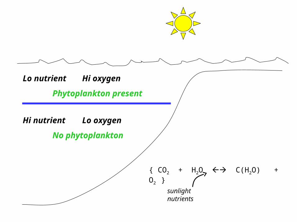
Lo nutrient Hi oxygen

Phytoplankton present

Hi nutrient Lo oxygen

No phytoplankton

Phytoplankton present

No phytoplankton

{ CO2 + H2O C(H2O) + O2 }

sunlight nutrients

Lo nutrient Hi oxygen

Phytoplankton present

Hi nutrient Lo oxygen

No phytoplankton

3 common problems in oceanography:

{ CO2 + H2O C(H2O) + O2 }

sunlight nutrients

Nutrient concentration: what does it really tell us?

Advection vs. growth: how do you differentiate?

µ = delta P / [P * time] we can’t easily measure it!

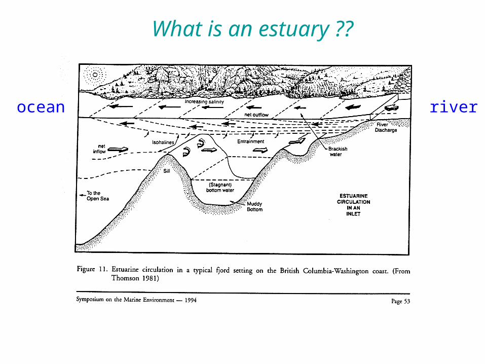
riverocean

What is an estuary ??

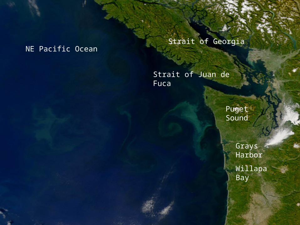
Grays Harbor

Willapa Bay

Strait of Juan de Fuca

Puget Sound

NE Pacific OceanStrait of Georgia

Re Puget Sound

• Dynamic and diverse• Scales of variation:

– temporal– spatial

• Boundary conditions:– ocean, river, atmosphere

• Drivers of change:– Climate– Humans

• Investigative tools:– Monitoring – Observing – Time-Series– Models, Experimentation

Pacific climate variability, 1900-1998

Steven Hare, UW, 1999

-40

-30

-20

-10

0

10

20

30

90 91 92 93 94 95 96 97 98 99 00

Southern Oscil. Indexmontly mean

ENSO during the last decade

NOAA

April 1999

April 1998

Ocean properties are not “constant”...

110 m

10 m

Smith et al. 2000

Dep

th (

m)

Dep

th (

m)

Distance from shore (km)

The depth of the thermocline was much deeper following El Niňo than La Niňa.

This affects not only the temperature but also the nutrients available at the surface.

In fact, we did find more phytoplankton on the coast during summer of 1999 than 1998.

Effect of a drought on river flow…

USGS, 2000

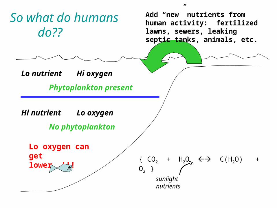
Lo nutrient Hi oxygen

Phytoplankton present

Hi nutrient Lo oxygen

No phytoplankton

{ CO2 + H2O C(H2O) + O2 }

Add “new” nutrients from human activity: fertilized lawns, sewers, leaking septic tanks, animals, etc.

So what do humans do??

Lo oxygen can get lower !!!

*sunlight nutrients

Lo nutrient Hi oxygen

Phytoplankton present

Hi nutrient Lo oxygen

No phytoplankton

{ CO2 + H2O C(H2O) + O2 }

Add “new” nutrients from human activity: fertilized lawns, sewers, leaking septic tanks, animals, etc.

So what do humans do??

Lo oxygen can get lower !!!

*

sunlight nutrients

Overarching Goal“Through a strongly interacting combination of direct observations and computer models representing physical, chemical, and biological processes in Puget Sound, provide a record of Puget Sound water properties, as well as model now-casts and projections.

The information will be used to develop a mechanistic understanding of the Sound’s dynamics, how human actions and climate influence these (e.g., “what-if scenarios”), and how, in turn, water properties influence marine resources and ecosystem health (linkage with other PRISM elements).”

Key questions

• Understanding plankton dynamics in a temperate fjord:- What physical dynamics of water mass variation most influence stratification, and what is the phytoplankton response?- How important is nitrate versus ammonium in controlling phytoplankton production?- What controls light availability for phytoplankton in the euphotic zone?

• Assessing ecosystem integrity:- Do salmon have food they need to survive? Is timing ok and what affects that?- What food-web shifts (e.g., macrozoops vs. gelatinous) affect fish etc survival?- How does an invasive species with certain growth/grazing characteristics impact food-web?

• Understanding perturbation impacts (e.g., climate, human):- How does productivity differ with ENSO and PDO stages?- How does flushing differ with ENSO and PDO stages?- Do land-use practices affect water properties and phytoplankton?

Uses and benefits

• The information will be used– for teaching at various levels – to promote and aid research– to help define effective regional planning

• Public benefit includes:– Resource and habitat protection (e.g.,

clean water, fish, shellfish)– Waste/pollution planning and allocation– Puget Sound quality maintenance

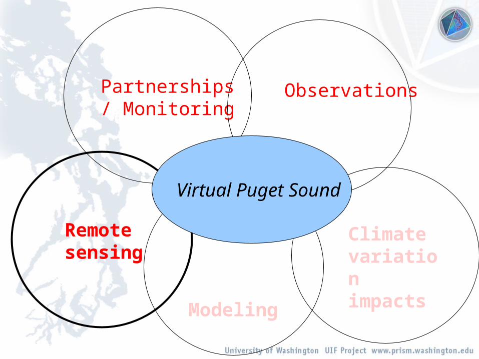
Climate variation impacts

Remote sensing

Modeling

ObservationsPartnerships/ Monitoring

Virtual Puget Sound

Climate variation impacts

Remote sensing

Modeling

ObservationsPartnerships/ Monitoring

Virtual Puget Sound

Ships & Buoys

Climate variation impacts

Remote sensing

Modeling

ObservationsPartnerships/ Monitoring

Virtual Puget Sound

DO FCB DIN NH4 Stratif Concern Budd Inlet Very Low High Low High PS. Hood Canal Very Low Low PPenn Cove Very Low Low PCommencement Bay Low Very High PElliott Bay Low Very High POakland Bay Very High Moderate Moderate EGrays Harbor Very High Moderate P-Eupper Willapa Bay Very High Low Moderate E-WPossession Sound Low High Moderate High PSinclair Inlet Low High Low Moderate PBellingham Bay Low Moderate Low Moderate PDrayton Harbor Moderate Low SN. Hood Canal Low Low PPort Orchard High Moderate SCase Inlet Low Moderate Moderate Moderate SCarr Inlet Low Moderate Moderate SQuartermaster Hbr Low Moderate STotten Inlet Moderate Moderate ESaratoga Passage Low Moderate PHolmes Harbor Low PSkagit Low PPort Susan Low PWest Point Moderate EDungeness Low SPort Gamble Low SSequim Bay Low SDiscovery Bay Low SWillapa Bay Low E-WDyes Inlet Moderate SEld Inlet Moderate SEast Sound High SBurley-Minter Moderate EPort Townsend Low WStrait of Georgia Low S

-123.5 -123.0 -122.5 -122.0

Longitude (deg)

47

48

49

La

titu

de

(d

eg

)

Marine Water Quality Index

Ships & Buoys

Climate variation impacts

Remote sensing

Modeling

ObservationsPartnerships/ Monitoring

Virtual Puget Sound

-123.5 -123.0 -122.5 -122.0

Longitude (deg)

47

48

49

La

titu

de

(d

eg

)

Marine Water Quality Index

Remote sensing

Ships & Buoys

Climate variation impacts

Remote sensing

Modeling

ObservationsPartnerships/ Monitoring

Virtual Puget Sound

-123.5 -123.0 -122.5 -122.0

Longitude (deg)

47

48

49

La

titu

de

(d

eg

)

Marine Water Quality Index

Willapa Integrated Primary Production

0

1000

2000

3000

4000

5000

6000

Oct-

97

No

v-9

7

Dec-9

7

Jan

-98

Feb

-98

Mar-

98

Ap

r-98

May-9

8

Ju

n-9

8

Ju

l-98

Au

g-9

8

Sep

-98

Oct-

98

No

v-9

8

Dec-9

8

Jan

-99

Feb

-99

Mar-

99

Ap

r-99

May-9

9

Ju

n-9

9

Ju

l-99

Au

g-9

9

Sep

-99

Oct-

99

No

v-9

9

Dec-9

9

mg

C m-2

d-1

Toke Pt. Bay Center Oysterville Naselle G-33

El Niño vs La Niña

Remote sensing

Ships & Buoys

Climate variation impacts

Remote sensing

Modeling

ObservationsPartnerships/ Monitoring

Virtual Puget Sound

-123.5 -123.0 -122.5 -122.0

Longitude (deg)

47

48

49

La

titu

de

(d

eg

)

Marine Water Quality Index

El Niño vs La Niña

Remote sensing

Ships & Buoys

Aquatic biogeochemical cycling model

DO FCB DIN NH4 Stratif Concern Budd Inlet Very Low High Low High PS. Hood Canal Very Low Low PPenn Cove Very Low Low PCommencement Bay Low Very High PElliott Bay Low Very High POakland Bay Very High Moderate Moderate EGrays Harbor Very High Moderate P-Eupper Willapa Bay Very High Low Moderate E-WPossession Sound Low High Moderate High PSinclair Inlet Low High Low Moderate PBellingham Bay Low Moderate Low Moderate PDrayton Harbor Moderate Low SN. Hood Canal Low Low PPort Orchard High Moderate SCase Inlet Low Moderate Moderate Moderate SCarr Inlet Low Moderate Moderate SQuartermaster Hbr Low Moderate STotten Inlet Moderate Moderate ESaratoga Passage Low Moderate PHolmes Harbor Low PSkagit Low PPort Susan Low PWest Point Moderate EDungeness Low SPort Gamble Low SSequim Bay Low SDiscovery Bay Low SWillapa Bay Low E-WDyes Inlet Moderate SEld Inlet Moderate SEast Sound High SBurley-Minter Moderate EPort Townsend Low WStrait of Georgia Low S

-123.5 -123.0 -122.5 -122.0

Longitude (deg)

47

48

49

La

titu

de

(d

eg

)

Marine Water Quality Index

Willapa Integrated Primary Production

0

1000

2000

3000

4000

5000

6000

Oct-

97

No

v-9

7

Dec-9

7

Jan

-98

Feb

-98

Mar-

98

Ap

r-98

May-9

8

Ju

n-9

8

Ju

l-98

Au

g-9

8

Sep

-98

Oct-

98

No

v-9

8

Dec-9

8

Jan

-99

Feb

-99

Mar-

99

Ap

r-99

May-9

9

Ju

n-9

9

Ju

l-99

Au

g-9

9

Sep

-99

Oct-

99

No

v-9

9

Dec-9

9

mg

C m-2

d-1

Toke Pt. Bay Center Oysterville Naselle G-33

El Niño vs La Niña

Remote sensing

Ships & Buoys

Aquatic biogeochemical cycling model

Climate variation impacts

Remote sensing

Modeling

ObservationsPartnerships/ Monitoring

Virtual Puget Sound

Observing Nutrient Dynamics PRISM Observations

• PRISM-sponsored cruises

• Partnership with WA Ecology and King Co DNR monitoring (PSAMP)

• JEMS: Joint Effort to Monitor the Strait,

co-sponsored by MEHP, et al.

• ORCA: Ocean Remote Chemical-optical Analyzer, initial sponsorship EPA/NASA, also WA SG, KC-DNR

• Annual June and Dec. cruises; 10 so far

• Greater Puget Sound including Straits

• Synoptic hydrographic, chemical, and biological data

• Input for models, student theses, regional assessments

PRISM cruises

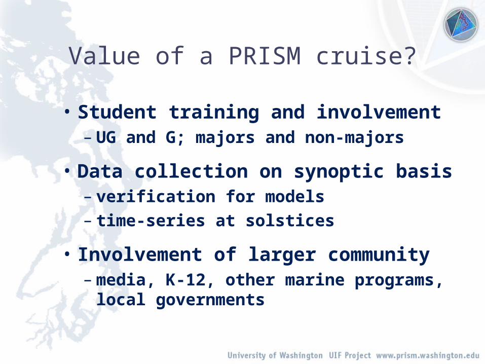
• Student training and involvement– UG and G; majors and non-majors

• Data collection on synoptic basis– verification for models– time-series at solstices

• Involvement of larger community– media, K-12, other marine programs, local

governments

Value of a PRISM cruise?

PRISM cruise participation:• UW Undergraduates - 34 persons, 60 trips (41%)

– Oceanography - 30– Other Majors - 4 [UW Tacoma , Biochemistry, Computer Sci, Fisheries]

• UW Grad Students- 21 persons, 23 trips (16%)– Oceanography - 11– Other Majors - 10 [Chem, Geol, Appl Math, Biol, Genetics, Sci Ed, Foriegn]

• WA State Dept. Ecology - 8 persons, 20 trips• UW Faculty - 4 persons, 13 trips• King County DNR - 4 persons, 5 trips• US Coast Guard Techs - 6 persons• Congressional Staff - 6 persons

• Media - 4 persons Totals : 94 persons, 146 trips• UW Staff - 3 persons 57% student labor• CORE - 2 persons• NOAA/PMEL - 1 person• Ocean Inquiry Project - 1 person• High School Teacher - 1 person

Data after 7 cruises:

PRISM Observations:

Hood Canal Oxygen and Ammonium

JEMS line

Joint Effort to Monitor the Strait(JEMS)

King County

MEHP

PRISM

Ecology

NOAA

Friday Harbor Labs

JEMS visits the three stations monthly.

Data collection began September 1999 and is ongoing.

sensor profiles- Temperature- Salinity- Density- Oxygen- Chlorophyll a

bottle samples (0, 30, 80, 140 m)

- Oxygen- Nutrients- Chlorophyll a

net tows- Plankton- Larvae

S O N D J F M A M J J A S O N D J F M A M J J A S O N D J F M A

0

50

100

150

Dep

th (

m)

Station 0 Temperature (oC)

7.5

8

8

88

8

8

8

8

8.5

8.5

8.5

8.5

8.5

8.5

9

9

9

9

9

9

9.5

9.5 9.

5

9.5

9.5

10 10

10

10.5

11

11.5

2000 2001 2002

S O N D J F M A M J J A S O N D J F M A M J J A S O N D J F M A

0

50

100

150D

epth

(m

)

Station 1 Temperature (oC)

7.5

8

888

8

8

8 8

8

8.5 8.5

8.5

8.5

8.5

8.5

8.5

9

9

9 9

9

9.5

9.5

9.5

9.5

10

10

1010

.5

11

2000 2001 2002

S O N D J F M A M J J A S O N D J F M A M J J A S O N D J F M A

0

50

100

150

Dep

th (

m)

Station 2 Temperature (oC)

8

8

88 8

8 88

8

8.5

8.5

8.5

8.5

8.5

8.5

9

9

9

9

9

9.5

9.5

9.5

9.510

10

10

10.5 10.511

2000 2001 2002

Temperature

With 2 1/2 years of data we can begin to study the interannual variation of water properties passing through the Strait and into the Puget Sound.

Determining the inter-annual variation of water properties in the Strait is necessary for understanding variation in San Juans and Puget Sound.

S O N D J F M A M J J A S O N D J F M A M J J A S O N D J F M A

0

50

100

150

Dep

th (

m)

Station 0 Salinity (PSU)

30

3030.5

30.5

30.5

30.5

3131

31

31

31

31

3131

31

31.5

31.5 31.5

31.5

31.5

31.5

32

32

32 32

32

32

32

32.5 32.5 32.5

2000 2001 2002

S O N D J F M A M J J A S O N D J F M A M J J A S O N D J F M A

0

50

100

150D

epth

(m

)

Station 1 Salinity (PSU)

30

30

30.5

30.5 30

.5

30.5

30.531

31

31

31

31 31

31

31.5

31.5

31.5

31.5 31.5

31.5

31.5

32

32

32

32

32

32

32

32.5

32.5 32

.5

33 33

33

2000 2001 2002

S O N D J F M A M J J A S O N D J F M A M J J A S O N D J F M A

0

50

100

150

Dep

th (

m)

Station 2 Salinity (PSU)

30

3030

30.5

30.5 30.531

3131

31

31

31

31.5

31.5

31.531.5

31.5

32

32

32

32

32

32

32

32.5

32.5

32.5

32.5

32.5

32.5

33

33

33

33 33

33.5

2000 2001 2002

SalinityLocal:High salinity at depth on US side.Low salinity at surface on Canadian side.

Annual:Low salinity water mixes down during winter.High salinity water enters during summer.

Interannual:2000-2001 drought is easily observed.

S O N D J F M A M J J A S O N D J F M A M J J A S O N D J F M A

0

50

100

150

Depth

(m

)

Station 0 Temperature (oC)

8

9

2000 2001 2002

S O N D J F M A M J J A S O N D J F M A M J J A S O N D J F M A

0

50

100

150

Depth

(m

)

Station 1 Temperature (oC)88.5

2000 2001 2002

S O N D J F M A M J J A S O N D J F M A M J J A S O N D J F M A

0

50

100

150

Depth

(m

)

Station 2 Temperature (oC)

8

2000 2001 2002

S O N D J F M A M J J A S O N D J F M A M J J A S O N D J F M A

0

50

100

150

Depth

(m

)

Station 0 Salinity (PSU)

2000 2001 2002

S O N D J F M A M J J A S O N D J F M A M J J A S O N D J F M A

0

50

100

150

Depth

(m

)

Station 1 Salinity (PSU)

2000 2001 2002

S O N D J F M A M J J A S O N D J F M A M J J A S O N D J F M A

0

50

100

150

Depth

(m

)

Station 2 Salinity (PSU)

2000 2001 2002

Temperature

Salinity

Compare Sept 2000 with Sept 2001

Q1: What effects can we expect from climate variation ??

How did the environment vary in 2000 vs. 2001?

Air Temperature:No apparent difference

Sunlight:No apparent difference

Upwelling:No apparent difference

River Discharge:Drought, Fall 2000 Increased flow, Fall 2001

S O N D J F M A M J J A S O N D J F M A M J J A S O N D J F M A0

500

1000

1500

2000

2500Skagit River Discharge

Riv

er D

isch

arge

(m

3/s

)

2000 2001 2002

Skagit River Discharge

fresher, warmer water from Sound and San Juans flowing out colder, salty

water from Pacific Ocean flowing in

North Canada

South U.S.A.

Cross-Channel Density Gradient

9/2/99

Dep

th (

m)

0 1 2

20406080

100120140

10/15/99

0 1 2

20406080

100120140

11/23/99

0 1 2

20406080

100120140

12/20/99

0 1 2

20406080

100120140

1/27/00

Dep

th (

m)

0 1 2

20406080

100120140

2/12/00

0 1 2

20406080

100120140

3/5/00

0 1 2

20406080

100120140

3/29/00

0 1 2

20406080

100120140

5/2/00

Dep

th (

m)

0 1 2

20406080

100120140

7/5/00

0 1 2

20406080

100120140

8/31/00

0 1 2

20406080

100120140

11/14/00

0 1 2

20406080

100120140

1/15/01

Dep

th (

m)

0 1 2

20406080

100120140

3/23/01

0 1 2

20406080

100120140

6/25/01

0 1 2

20406080

100120140

7/29/01

0 1 2

20406080

100120140

9/13/01

Station

Dep

th (

m)

0 1 2

20406080

100120140

1/30/02

Station0 1 2

20406080

100120140

3/25/02

Station0 1 2

20406080

100120140

Colorbar

Density (sigma-t)22

26

North South

Warmer fresher water drives stronger density gradient during Sep 2001 than in Sep 2000

S O N D J F M A M J J A S O N D J F M A M J J A S O N D J F M A

0

20

40

60

80

100

Depth

(m

)

Geostrophic Velocity (cm/s)

0

2000 2001 2002

Geostrophic Velocity

High River Flow

Large Cross-

Channel Gradient

Increased Geostrophic

Out Flow

Decreased Residence

Time2000 drought had consequences…

Areas of know n low D O (ye llow = b io logica l stress; red = hypoxia), and areas w ith susceptib ility to eutrophication (p ink) on physica l/chem ical characteristics.

Marine W ater Quality Status and Susceptibility

Partnership: Ecology PSAMP monitoring

• Analysis of monitoring data identified South Puget Sound as an area susceptible to eutrophication

• Led to focused study on South Sound nutrient sensitivity (SPASM)

• Coordination of SPASM and PRISM modeling/observ.

http://www.ecy.wa.gov/

Q2: Where is Puget Sound most sensitive to nutrient loading and are affects being seen ??

4625

3225

3412

2900

2360

19832340

2186

1500

~3000

~2000

n=19

n=19

n=5 x 80

n=30

n=8

Primary Production (mg C m-2 d-1)

>1000-2000 >2000-3000 >3000-4000 >4000-5000

Newton et al., 2001

32/79

28/78

13/17

10/16

15/209/14

4/11

11/152

15/51

% increase in integrated / surface prod’n

<5 / <10 >5-15 / >10-30 >15-25 / >30-50 >25-35 / >50-70 >35 / >70

Newton et al., 2001

-100

0

100

200

300

400

500

600

Jan Feb Mar Apr May Jun Jul Aug Sep Oct Nov Dec

Per

cen

t in

crea

se i

n s

urf

ace

pro

du

ctio

n

Hood Canal

South Sound

Central Basin

Effect of added nutrients:

Newton et al., 2001

July 12 - 28, 2000

enhancement

October 15-21, 2000Sept. 20- Oct. 2, 2000

no enhancement surface enhancement

Sigma-t

Chl ug/l

O2 mg/l

enhancement no enhancement surface enhancement

0

5

10

15

0 500 10000

5

10

15

20

25

0 500 10000

5

10

15

0 200 400 600

12 Oct 0025 Sep 0010 Jul 00

dep

th (

m)

primary productivity (mg C m-3 d-1)

Effect of nutrient addition on phytoplankton productivity

blue = ambient productionred = spiked with NH4 & PO4

Carr Inlet, WA Ecology

Newton and Reynolds, 2002

ORCA website

July 12 - 28, 2000

enhancement

October 15-21, 2000Sept. 20- Oct. 2, 2000

no enhancement surface enhancement

Sigma-t

Chl ug/l

O2 mg/l

enhancement no enhancement surface enhancement

0

5

10

15

0 500 10000

5

10

15

20

25

0 500 10000

5

10

15

0 200 400 600

12 Oct 0025 Sep 0010 Jul 00

dep

th (

m)

primary productivity (mg C m-3 d-1)

Effect of nutrient addition on phytoplankton productivity

blue = ambient productionred = spiked with NH4 & PO4

Carr Inlet, WA Ecology

Newton and Reynolds, 2002

ORCA website

Partnership: KC-DNR’s WWTP siting

• Region’s growth is requiring greater capacity to treat wastewater. New WWTP proposed.

• KC MOSS study to site marine outfall and assess potential impacts

• Coordinated modeling and observ. effort with PRISM

http://www.metrokc.gov/

Marine outfall zones with depth contours

Q3: “What if” we built a new outfall in Central Puget Sound ??

Modeling Nutrient DynamicsPRISM Models

• POM model: Princeton Ocean model, hydrodynamics

• ABC model: Aquatic Biogeochemical Cycling

ABC Model

What is an Aquatic Biogeochemical Cycling Model and why develop one

for PRISM?

• Describes the dynamics of nutrients, plankton, and organic material in a water column; this has defining importance for water quality, food for higher trophic levels, and change impact projections.

• Water quality models commonly in use take more of a curve-fitting approach, are composed of antiquated coding, and do not support teaching as well.

• The model is an essential tool for exploring the fundamentals of biogeochemical cycling in Puget Sound, for use in planning or ”what-if” scenarios, and for use in teaching and communication.

ABC model development

• Identified the need• Design box and wire• Mathematically define transfer processes• Develop model architecture and code• Create GUI• Test (Ocean 506b)• Interface with hydrodynamic model

ABC model development

• Phytoplankton– Reynolds, Newton

• Zooplankton– Gentleman, Leising

• Nutrients/organics– Devol

• Oxygen– Warner

• Hydrodynamics– Kawase, Albertson, Nairn

• Light– Reynolds

• Model coding– Davis– Serper

• Model architecture– Logsdon

• Model implementation– Nairn

• Model integration– Averill– Nairn– Logsdon

Aquatic Biogeochemical Cycling Model: Features

• Under active development (UW, WDOE, KCDNR)• Simulates three-dimensional concentrations of

chemical and biological entities:• Dissolved oxygen and nutrients (NO3, PO4, NH4)

• Phytoplankton biomass (three types)• Zooplankton biomass (three types)• Particulate and dissolved organic matter (C, N, P)

• Externally forced by hydrodynamics and sunlight• Designed to interface with a variety of circulation models

including POM, linkage to MM-5 and SWIM

• Spatially explicit model based on published equations for biological and chemical reactions

Biogeochemical Systems ModelrPON rPOP

lPOC lPON lPOP

DOC DON DOP

O2

NO3

NH4

PO4

Z1ic Z2mac Z3gel

P1flag P2dia P3nan

rPOC

19 state variables

48 transfer processes

State Variables:

P1, P2, P3:

dPi/dt = psP-O2 – prO2-P – hgP-Z – peP-DOM – pdP-r,lPOM – csP-out

growth – respiration – grazing – exudation – cell death – cell sinking

 

Z1, Z2, Z3:

dZi/dt = – zrO2-Z – zdZ-DOM – zeZ-r,lPOM – zpZ-out – zmZ-r,lPOM + zg[P,Z,r,lDOM]-Z

– cgZ-Z + zsZ-Z

– respiration – exudation – egestion – predation – mortality

+ grazing – carnivory + swimming 

NH4:

dNH4/dt = neP-NH4 + nxZ-NH4 + bm[DOM,r,lPOM]-NH4 – nuNH4-P – niNH4-NO3

  phytopk excretion + zoopk excretion + bacterial

remineralization – nutrient uptake – nitrification

NO3:

dNO3/dt = niNH4-NO3 - nuNO3-P

nitrification – nutrient uptake

{airborne deposition, precipitation at surface}

Biogeochemical Systems ModelrPON rPOP

lPOC lPON lPOP

DOC DON DOP

O2

NO3

NH4

PO4

Z1ic Z2mac Z3gel

P1flag P2dia P3nan

rPOC

Transfer Processes: ps: photosynthesis (16)

 

ps = Pi oi eRiT min { rll, rnuN, rnuP }

where: oi = maximal growth rate for Pi = oiTbase * e-Ri*Tbase

oiTbase = maximal growth rate for Pi at Tbase

Tbase = base temperature Ri = temperature growth coefficient for Pi T = temperature (input) rll, rnuN, rnuP = resource limitation factors: relative degree

of growth limitation due to light, nutrient uptake for N, or for P  

Resource limitation factors:

rll= 1 - e –Eki/E   target theory for photosynthesis Eki = light saturation coefficient for Pi

E = light (input)

rnuN = rnuNH4 + rnuNO3

rnuP = rnuPO4

rnuNH4 = NH4 Monod function Ki NH4 + NH4

 

rnuNO3 = NO3 * Ki NH4 ammonium

Ki NO3 + NO3 Ki NH4 + NH4 inhibition term 

Ki[nutr] = half saturation constant for Pi on nutrient [NO3, NH4, PO4]

Nitrate [µM]Irradiance [µmol m-2 s-1]

Tem

pera

ture

[°C

]

Phytoplankton specific-growth rate, d-1

R. Reynolds

Biogeochemical Systems ModelrPON rPOP

lPOC lPON lPOP

DOC DON DOP

O2

NO3

NH4

PO4

Z1ic Z2mac Z3gel

P1flag P2dia P3nan

rPOC

nu: nutrient uptake (13a, b, c) from NO3, NH4, PO4 to Pi

 

nu NH4-P = ps / stoich(C:N)2 * rnuNH4

rnuNH4 + rnuNO3

 

nu NO3-P = ps / stoich(C:N)1 * rnuNO3

rnuNH4 + rnuNO3

 

nu NO3-O2 = nu NO3-P / stoich(N:O)1

(to account for O2 produced during assimilative nitrate reduction) nu PO4-P = ps / stoich(C:P)1

where: rnuNH4 = NH4

Ki NH4 + NH4

 rnuNO3 = NO3 * Ki NH4

Ki NO3 + NO3 Ki NH4 + NH4

 Ki[nutr] = half saturation constant for Pi on nutrient [NO3, NH4, PO4]

Biogeochemical Systems ModelrPON rPOP

lPOC lPON lPOP

DOC DON DOP

O2

NO3

NH4

PO4

Z1ic Z2mac Z3gel

P1flag P2dia P3nan

rPOC

hg: herbivorous grazing (1-9) from Pi to Zi; i = 1-3; j = 1-3

 

hgP-Z = P1g + P2g + P3g

Pig = Zj * Imax * max (B - Co, 0) * j Pi * O2 .

KiA + B A KiO2 + O2

where: Imax = maximal ingestion rate = ImaxTbase * e-fz(T)*Tbase

ImaxTbase = maximal ingestion rate at Tbase

Tbase = base temperatureCo = feeding threshold level, below which no grazing occursj = preference for prey type, j=1-8: 1=P1, 2=P2, 3=P3, 4=Z1, 5=Z2, 6=Z3, 7=lPOM, 8=rPOMKiA = half-saturation constant for total food

KiO2 = half saturation constant for Zi on O2

A = total food available = 1*P1 + 2*P2 + 3*P3 + 4*Z1 + 5*Z2 + 6*Z3 + 7*lPOM + 8*rPOM

B = total food = P1 + P2 + P3 + Z1 + Z2 + Z3 + lPOM + rPOM

 

Can run in Chemostat mode

0

1

2

3

4

5

6

7

8

9

10

0 100 200 300 400 500 600

time (days)

NO3

Diatoms

Copepods

1-cell ABC model output, constant light, no mixing

0

1

2

3

4

5

6

7

8

9

10

0 100 200 300 400 500 600

time (days)

NO3

Diatoms

Copepods

Jellyfish

DON

But want multi-cell resolution with hydrodynamics

Run coupled ABC-POM

Test in Budd Inlet

Previous EFDC model runs and field data

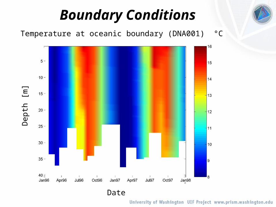
Model Inputs

SW Rad [W m-2]

Air Temp [°C]

Rel. Humidity [%]

River Flow [m3 s-1]

Date

De

pth

[m]

Temperature at oceanic boundary (DNA001) °C

Boundary Conditions

Surface

Bottom

Te

mp

era

ture

[°C

]Data comparisons

Northing (km)1 9

Dep

th (

m)

0

14

degrees C

Longitudinal section of temperature in Budd Inlet

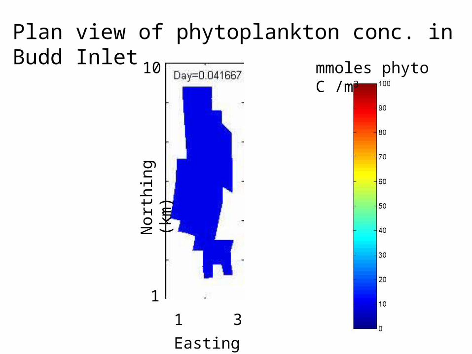
mmoles phyto C /m3

Plan view of phytoplankton conc. in Budd Inlet

Easting (km)

1

1

10

3

Nor

thin

g (k

m)

Aquatic Biogeochemical Cycling Model: Applications

• Primary applications are to assess:– dynamics of phytoplankton blooms (eutrophic’n, HABs)

– dynamics of dissolved oxygen and water quality

– sensitivity to changes, both human (e.g., WWTP, climate change) and natural (e.g., ENSO, regime shift)

• Suitable for both marine and freshwater systems• Supports linkages; will provide output to

– nearshore sediment-biological model

– higher trophic level models (e.g., salmon!)

• Same tool can be used for teaching, basic research, applied research, and planning decisions.

Aquatic Biogeochemical Cycling Model: Status

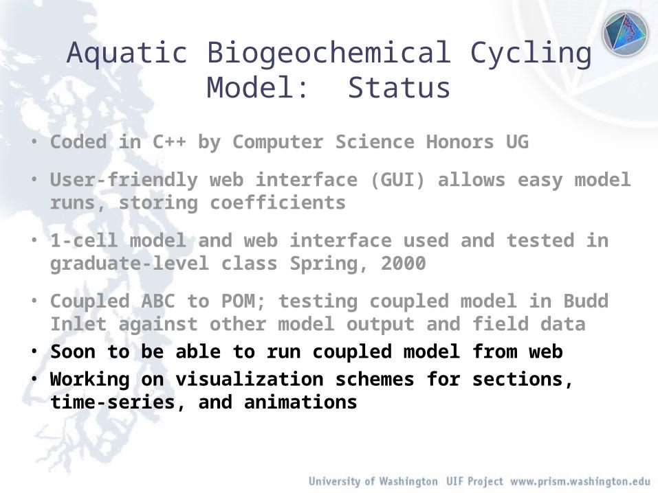
• Coded in C++ by Computer Science Honors UG

• User-friendly web interface (GUI) allows easy model runs, storing coefficients

• 1-cell model and web interface used and tested in graduate-level class Spring, 2000

• Coupled ABC to POM; testing coupled model in Budd Inlet against other model output and field data

• Soon to be able to run coupled model from web

• Working on visualization schemes for sections, time-series, and animations

Goals for achieving VPS

• Internal to ABC:– Sediment module

• ABC needs directly:– POM (hydrodynamics)

• DSHVM (river input)• MM-5 (weather forcings)

• ABC can support:– Sediment/toxics transport and fate– Nearshore processes (NearPRISM)– Upper trophic levels (e.g., fish management)– HABs

MEPS:“A Partnership for Modeling the Marine

Environment of Puget Sound, Washington”

NOPP / PRISMKawase et al.

Develop, maintain and operate a system of simulation models of Puget Sound’s circulation and ecosystem, a data management system for oceanographic data and model results, and an effective delivery interface for the model results and observational data for research, education and policy formulation.

MIXED

Model/measurementIntegration

eXperiment in Estuary

Dynamics

A PRISM project

Motivation

• Study coupled ecosystem of south Sound– Biology, chemistry, circulation, runoff, weather

– Water quality vulnerability

• Integrate, validate PRISM models– Preparation for other studies; domain is entire Sound

– Virtual Puget Sound, bloodstream

• Education– Oceanography fieldwork class

– Oceanography of Puget Sound class

SPASM

Car

r

MIXED components

• BioFloat - D’Asaro, Reynolds– O2, chlorophyll following water parcel: biological productivity

• Surveys – Reynolds, Newton– O2, chlorophyll, nutrients, productivity

• Integrated physical model - Kawase, Edwards

• Aquatic Biogeochemistry Model – al.

• ORCA - Devol, Emerson

• PRISM - Richey et al.

• Ocean Students

When: next Spring bloom

Plots from ORCA, USGS websites; data from NDBC.

Streamflow

Win

d s

pe

ed

(m

/s) A

ir tem

p. (C

)

Conclusions

• Puget Sound shows strong temporal and spatial variation re nutrient dynamics

• Region has sensitivity to climate and human perturbations

• Combined observations and modeling are needed to answer questions