Modeling And Predictive Control Of High Performance Buildings 

With Distributed Energy Generation And Thermal Storage

Siwei Li, Jaewan Joe, Panagiota KaravaLyles School of Civil Engineering (ArchE Group)

Purdue University

IntroductionObjectivesOverview

Integrated modellingSolar SystemBuilding Model

System Identification Gray‐BoxSubspace Algorithm (Black‐Box) 

Results and AnalysisMPC SimulationEnergy Saving Potential

Conclusions2

OUTLINE

3

OUTLINE

IntroductionObjectivesOverview

Integrated modellingSolar SystemBuilding Model

System Identification Gray‐BoxSubspace Algorithm (Black‐Box) 

Results and AnalysisMPC SimulationEnergy Saving Potential

Conclusions

Objectives

4

Develop models that capture the relevant system dynamics and are computationally efficient for subsequent use within model‐predictive control (MPC) algorithms.

Investigate the energy saving potential of the integrated system and the predictive controller in comparison with baseline operation strategies.

5

OverviewGrid

Building

Solar irradiance

Utility price

Electricity energy flows Thermal flow Environmental disturbances

Heat pump

Ventilation

Heating load

Radiant floor heating

TBIPV/TTBIPV/T

Ttank

qHP

Thermal storage

HVAC

BIPV/T

Occupancy Weather

6

Grid

Solar irradiance

Utility price

Electricity energy flows Thermal flow Environmental disturbances

Radiant floor heating

TBIPV/T

Ttank

qHP

Thermal storage

Occupancy Weather

Overview

Heat pump

Ventilation

Heating loadBIPV/T

7

Approach

CFD simulation

Experiments

Energy simulation –thermal network

Parametric study

Airflow and thermal field analysis

Nu correlations

Integrated energy model

Test-bed:Living Lab

Building systems integration & Model-predictive Control

ValidateValidate

Input

Coupled with TRNSYS

Assumptions

Weather data

Weather forecastuncertainty

Overview

8

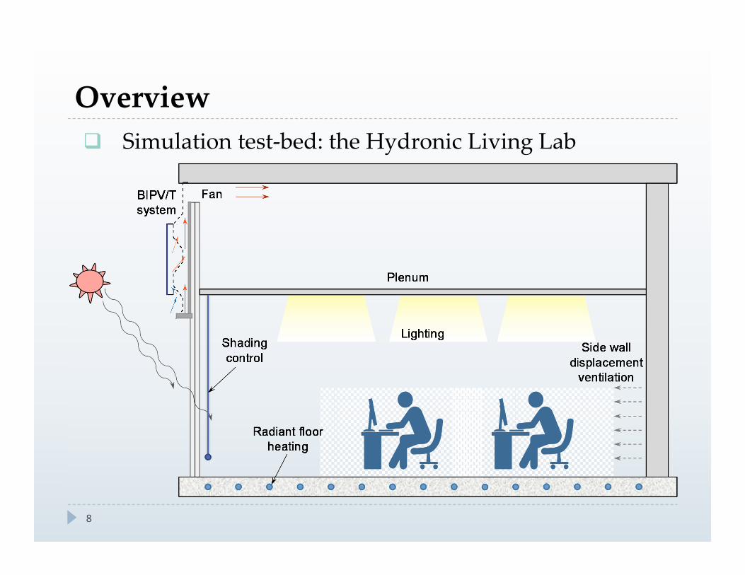
Simulation test‐bed: the Hydronic Living Lab

Overview

9

OUTLINE

IntroductionObjectivesOverview

Integrated modellingSolar SystemBuilding Model

System Identification Gray‐BoxSubspace Algorithm (Black‐Box) 

Results and AnalysisMPC SimulationEnergy Saving Potential

Conclusions

10

The corrugated transpired solar collector (without (left) and with (right) PV panels)

fan

cold air

solar radiation

Adiabatic w

all

Corrugated UTC

fan

cold air

solar radiation

UTC

PV module

Adiabatic w

all

Solar System

Building Model

11

Simulation test‐bed: the Hydronic Living Lab

User‐defined component

Building Model

12

Room 

Temperature

18 – 26 °C, 8:00 am – 10:00 am

21 – 26 °C, 10:00 am – 18:00 pm

>15 °C, 18:00 pm – 8:00 am

Floor 

Temperature19 – 29 °C (ASHRAE Standard 55)

Blind controlON, when the incident solar radiation on the window exceeds 180 W/m2

OFF, when the incident solar radiation on the window drops below 160 W/m2

BIPV/T

design

Total area: 65 m2

PV area: 58.5 m2, around 6.32 kWp

Air flow rate: 5,600 m3/hr, corresponding suction velocity: 0.024 m/s

13

OUTLINE

IntroductionObjectivesOverview

Integrated modellingSolar SystemBuilding Model

System Identification Gray‐BoxSubspace Algorithm (Black‐Box) 

Results and AnalysisMPC SimulationEnergy Saving Potential

Conclusions

Gray‐Box

14

State Space 4th order Linear Time‐invariant Discrete

x: state vector (= y)u: input vectory: output vectorA, B, C, D, K: unknowns need to be identified

Ttank

Ctank

ta

Ta2 +-

Uft

qhpCfloorCroom

Urf

Tfloor

TroomUre

qSG2

Cenve

Tenve

Ta+-

Uea

qSG

qSG3

Uef

Ura

Ta3+ -Ufa

U

Identification1

15

10 1010 1010 1010 1010 1010 1010 1010 10

10 1010 1010 1010 10

Gray‐Box

Cost Function:

Subject to:

Optimization algorithm: GA

Identification

Training data set: 49 days (Jan 3rd – Feb 24th)

Calibration data set: 7 days (Feb 25th‐Mar 3rd)

16

Tenve Troom Tfloor Ttank

Training Data‐RMSE (°C) 0.48 0.62 0.84 0.39

Calibration Data‐RMSE (°C) 0.59 0.61 0.98 0.55

Gray‐BoxResults

15

25

35

45

55

2/25

2/26

2/27

2/28

2/29

3/1

3/2

Temperature [degC]

Troom‐Reduced‐order SS model Troom‐TRNSYS modelTtank‐Reduced‐order SS model Ttank‐TRNSYS model

17

Subspace State‐Space System Identification (4SID)

4SIDqSG

TenveTroomTfloorTwrTtank

qSG2

qSG3

qhp

Ta

Ta2

Orders: 20 Inputs: 6; Outputs: 5;  Training data set: 49 days 

(Jan 3rd – Feb 24th) Calibration data set: 7 days 

(Feb 25th‐Mar 3rd)

x: state vectoru: input vectory: output vectorA, B, C, D, K: unknowns need to be identified

1

zero

18

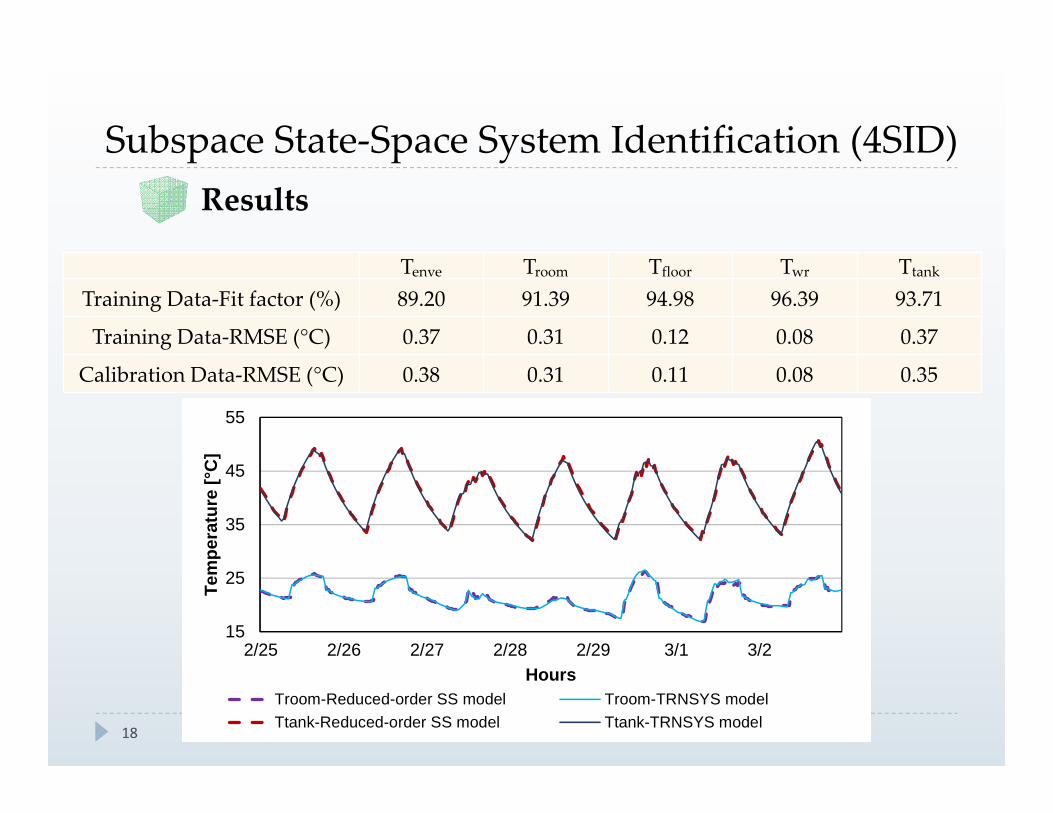
Tenve Troom Tfloor Twr Ttank

Training Data‐Fit factor (%) 89.20 91.39 94.98 96.39 93.71

Training Data‐RMSE (°C) 0.37 0.31 0.12 0.08 0.37

Calibration Data‐RMSE (°C) 0.38 0.31 0.11 0.08 0.35

Subspace State‐Space System Identification (4SID)Results

15

25

35

45

55

2/25 2/26 2/27 2/28 2/29 3/1 3/2

Tem

pera

ture

[°C

]

HoursTroom-Reduced-order SS model Troom-TRNSYS modelTtank-Reduced-order SS model Ttank-TRNSYS model

19

OUTLINE

IntroductionObjectivesOverview

Integrated modellingSolar SystemBuilding Model

System Identification Gray‐BoxSubspace Algorithm (Black‐Box) 

Results and AnalysisMPC SimulationEnergy Saving Potential

Conclusions

20

MPC SimulationRead the TMY3 data as the weather forecast

Input the initial states of the building (5 temperatures)

Propose a heuristic initial guess for the control variable qhp

Substitute the control variable into the simplified model and apply the optimization algorithm to

explore and assess the potential solutions for qhp• Ensure no violations of the environmental

(temperatures) or equipment constraints• Calculate the cost function for different

sequences of the control variable

Select the sequence of the control variable with lowest cost function and output the corresponding set points of the tank

temperature

For online MPC, send the tank set point trajectory to the building automation system over the next 2 hours.

Recalculate the final states for the building and repeat the process every 2 hours.

Model-predictive controller

Flow chart:

21

∑ Cost Function:

MPC Simulation

∈ 0,∈ 25, 55∈ 19, 29

∈18,26 08:00 ~ 10:00) 21,26 10:00 ~ 18:00) 15,26 18:00 ~ 08:00) 

Optimization algorithm: Pattern search

Subject to: 

( )0 1 2 32

42

5

22

Three consecutive sunny days 

Total electrical energy consumption: 84 kWh

Corresponding heating load: 690.3 kWh

Equivalent COP: 8.22

MPC SimulationScenario 1

0

400

800

799 809 819 829 839 849 859 869Inci

dent

Sol

ar

Rad

iatio

n [W

/m2]

0

4000

8000

12000

799 809 819 829 839 849 859 869H

eatin

g P

ower

[W]

0

2000

4000

799 809 819 829 839 849 859 869

Ele

ctric

al

Pow

er [W

]

-15-55

15253545

799 809 819 829 839 849 859 869Tem

pera

ture

[°C

]

Hours

Ttank Troom Ta

23

Two sunny days and one cloudy day 

Total electrical energy consumption: 116 kWh(38% more than scenario1)

Corresponding heating load: 491.3 kWh

Equivalent COP: 4.24

MPC SimulationScenario 2

0

400

800

967 977 987 997 1007 1017 1027 1037Inci

dent

Sol

ar

Rad

iatio

n [W

/m2]

0

5000

10000

15000

965 975 985 995 1005 1015 1025 1035H

eatin

g Po

wer

[W]

0

2000

4000

965 975 985 995 1005 1015 1025 1035

Ele

ctric

al

Pow

er [W

]

-20-10

01020304050

965 975 985 995 1005 1015 1025 1035

Tem

pera

ture

[°C

]

Hours

Ttank Troom Ta

Energy Saving Potential

24

Two optimal trajectories for scenario one Total electrical energy consumption: 116 kWh vs. 84 kWh (34.5% more for red line)

15

20

25

30

799 809 819 829 839 849 859 869

Roo

m

Tem

pera

ture

[°

C]

2530354045

799 809 819 829 839 849 859 869

Tank

Te

mpe

ratu

re

[°C

]

0

4,000

8,000

12,000

799 809 819 829 839 849 859 869

Ele

ctric

al

Pow

er [W

]

Hours

25

Building heating load: 3896 kWh (February)

10.8 %

33.9 %

11.7 %17.4 %

45.4 %

Energy Saving Potential ‐One month Simulation

Conclusions

26

The developed low‐order models capture the control‐relevant system dynamics Gray‐box model: RMSE of 0.61°C and 0.55 °C  for the zone and 

tank temperature  Black‐box model: RMSE of 0.31°C and 0.35 °C  for the zone and 

tank temperature

Model‐predictive control is an efficient solution for the proposed solar system with hydronic floor and thermal storage Significant energy savings can be achieved (up to 34.5% based on 

the analysis for scenario 1 and 2) The total energy saving of the proposed system with MPC can be 

up to 45.4 % compared to baseline RFH operation.

27

Improve the solution algorithm for the nonlinear optimization problem.

Incorporate the water flow rate as a control variable to have a more precise control of the room temperature.

Investigate the weather forecast uncertainty modeling and propagation over the planning horizon.

Investigate the energy efficiency of the integrated system using other solar collectors.

Future Work

Acknowledgements

28

Purdue Research Foundation.  ASHRAE (New Investigator Award). 

29

Thank You !

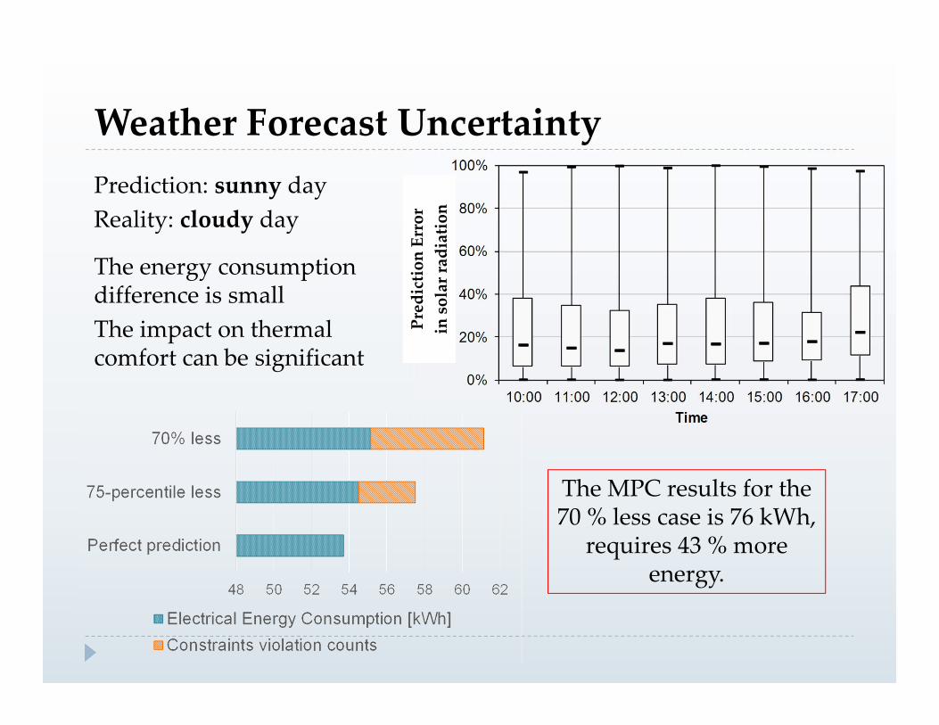
Prediction: sunny dayReality: cloudy day

The energy consumption difference is smallThe impact on thermal comfort can be significant

The MPC results for the 70 % less case is 76 kWh, 

requires 43 % more energy.

Weather Forecast Uncertainty

Prediction Error 

in solar radiation

Control In TRNSYS

Tankset‐pointtemp min Tout 50,55