Modeling and Rendering Architecture from Photographs

by

Paul Ernest Debevec

B.S.E. (University of Michigan at Ann Arbor) 1992B.S. (University of Michigan at Ann Arbor) 1992

A dissertation submitted in partial satisfaction of the

requirements for the degree of

Doctor of Philosophy

in

Computer Science

in the

GRADUATE DIVISION

of the

UNIVERSITY of CALIFORNIA at BERKELEY

Committee in charge:

Professor Jitendra Malik, ChairProfessor John CannyProfessor David Wessel

Fall 1996

Modeling and Rendering Architecture from Photographs

Copyright Fall 1996

by

Paul Ernest Debevec

1

Abstract

Modeling and Rendering Architecture from Photographs

by

Paul Ernest Debevec

Doctor of Philosophy in Computer Science

University of California at Berkeley

Professor Jitendra Malik, Chair

Imagine visiting your favorite place, taking a few pictures, and then turning those pictures

into a photorealisic three-dimensional computer model. The work presented in this thesis combines

techniques from computer vision and computer graphics to make this possible. The applications

range from architectural planning and archaeological reconstructions to virtual environments and

cinematic special effects.

This thesis presents an approach for modeling and rendering existing architectural scenes

from sparse sets of still photographs. The modeling approach, which combines both geometry-based

and image-based techniques, has two components. The first component is an interactive photogram-

metric modeling method which facilitates the recovery of the basic geometry of the photographed

scene. The photogrammetric modeling approach is effective, convenient, and robust because it ex-

ploits the constraints that are characteristic of architectural scenes. The second component is a model-

based stereo algorithm, which recovers how the real scene deviates from the basic model. By mak-

2

ing use of the model, this new technique robustly recovers accurate depth from widely-spaced im-

age pairs. Consequently, this approach can model large architectural environments with far fewer

photographs than current image-based modeling approaches. For producing renderings, this thesis

presents view-dependent texture mapping, a method of compositing multiple views of a scene that

better simulates geometric detail on basic models.

This approach can be used to recover models for use in either geometry-based or image-

based rendering systems. This work presents results that demonstrate the approach’s ability to create

realistic renderings of architectural scenes from viewpoints far from the original photographs. This

thesis concludes with a presentation of how these modeling and rendering techniques were used to

create the interactive art installation Rouen Revisited, presented at the SIGGRAPH ’96 art show.

Professor Jitendra MalikDissertation Committee Chair

iii

To Herschel

1983 - 1996

iv

Contents

List of Figures vii

List of Tables ix

1 Introduction 1

2 Background and Related Work 82.1 Camera calibration . . . . . . . . . . . . . . . . . . . . . . . . . . . . . . . . . . 82.2 Structure from motion . . . . . . . . . . . . . . . . . . . . . . . . . . . . . . . . . 92.3 Shape from silhouette contours . . . . . . . . . . . . . . . . . . . . . . . . . . . . 102.4 Stereo correspondence . . . . . . . . . . . . . . . . . . . . . . . . . . . . . . . . 152.5 Range scanning . . . . . . . . . . . . . . . . . . . . . . . . . . . . . . . . . . . . 182.6 Image-based modeling and rendering . . . . . . . . . . . . . . . . . . . . . . . . . 18

3 Overview 22

4 Camera Calibration 254.1 The perspective model . . . . . . . . . . . . . . . . . . . . . . . . . . . . . . . . 254.2 How real cameras deviate from the pinhole model . . . . . . . . . . . . . . . . . . 284.3 Our calibration method . . . . . . . . . . . . . . . . . . . . . . . . . . . . . . . . 314.4 Determining the radial distortion coefficients . . . . . . . . . . . . . . . . . . . . 314.5 Determining the intrinsic parameters . . . . . . . . . . . . . . . . . . . . . . . . . 384.6 Working with uncalibrated images . . . . . . . . . . . . . . . . . . . . . . . . . . 39

5 Photogrammetric Modeling 425.1 Overview of the Facade photogrammetric modeling system . . . . . . . . . . . . . 455.2 The model representation . . . . . . . . . . . . . . . . . . . . . . . . . . . . . . . 47

5.2.1 Parameter reduction . . . . . . . . . . . . . . . . . . . . . . . . . . . . . 475.2.2 Blocks . . . . . . . . . . . . . . . . . . . . . . . . . . . . . . . . . . . . 485.2.3 Relations (the model hierarchy) . . . . . . . . . . . . . . . . . . . . . . . 515.2.4 Symbol references . . . . . . . . . . . . . . . . . . . . . . . . . . . . . . 525.2.5 Computing edge positions using the hierarchical structure . . . . . . . . . 525.2.6 Discussion . . . . . . . . . . . . . . . . . . . . . . . . . . . . . . . . . . 54

v

5.3 Facade’s user interface . . . . . . . . . . . . . . . . . . . . . . . . . . . . . . . . 555.3.1 Overview . . . . . . . . . . . . . . . . . . . . . . . . . . . . . . . . . . . 555.3.2 A Facade project . . . . . . . . . . . . . . . . . . . . . . . . . . . . . . . 575.3.3 The windows and what they do . . . . . . . . . . . . . . . . . . . . . . . 575.3.4 The Camera Parameters Form . . . . . . . . . . . . . . . . . . . . . . . . 605.3.5 The Block Parameters form . . . . . . . . . . . . . . . . . . . . . . . . . 615.3.6 Reconstruction options . . . . . . . . . . . . . . . . . . . . . . . . . . . . 665.3.7 Other tools and features . . . . . . . . . . . . . . . . . . . . . . . . . . . 67

5.4 The reconstruction algorithm . . . . . . . . . . . . . . . . . . . . . . . . . . . . . 675.4.1 The objective function . . . . . . . . . . . . . . . . . . . . . . . . . . . . 675.4.2 Minimizing the Objective Function . . . . . . . . . . . . . . . . . . . . . 695.4.3 Obtaining an initial estimate . . . . . . . . . . . . . . . . . . . . . . . . . 70

5.5 Results . . . . . . . . . . . . . . . . . . . . . . . . . . . . . . . . . . . . . . . . . 725.5.1 The Campanile . . . . . . . . . . . . . . . . . . . . . . . . . . . . . . . . 725.5.2 University High School . . . . . . . . . . . . . . . . . . . . . . . . . . . 775.5.3 Hoover Tower . . . . . . . . . . . . . . . . . . . . . . . . . . . . . . . . 775.5.4 The Taj Mahal and the Arc de Trioumphe . . . . . . . . . . . . . . . . . . 79

6 View-Dependent Texture Mapping 816.1 Motivation . . . . . . . . . . . . . . . . . . . . . . . . . . . . . . . . . . . . . . . 816.2 Overview . . . . . . . . . . . . . . . . . . . . . . . . . . . . . . . . . . . . . . . 826.3 Projecting a single image onto the model . . . . . . . . . . . . . . . . . . . . . . . 83

6.3.1 Computing shadow regions . . . . . . . . . . . . . . . . . . . . . . . . . 846.4 View-dependent composition of multiple images . . . . . . . . . . . . . . . . . . 84

6.4.1 Determining the fitness of a particular view . . . . . . . . . . . . . . . . . 856.4.2 Blending images . . . . . . . . . . . . . . . . . . . . . . . . . . . . . . . 88

6.5 Improving rendering quality . . . . . . . . . . . . . . . . . . . . . . . . . . . . . 896.5.1 Reducing seams in renderings . . . . . . . . . . . . . . . . . . . . . . . . 896.5.2 Removal of obstructions . . . . . . . . . . . . . . . . . . . . . . . . . . . 896.5.3 Filling in holes . . . . . . . . . . . . . . . . . . . . . . . . . . . . . . . . 91

6.6 Results: the University High School fly-around . . . . . . . . . . . . . . . . . . . 926.7 Possible performance enhancements . . . . . . . . . . . . . . . . . . . . . . . . . 92

6.7.1 Approximating the fitness functions . . . . . . . . . . . . . . . . . . . . . 956.7.2 Visibility preprocessing . . . . . . . . . . . . . . . . . . . . . . . . . . . 95

7 Model-Based Stereo 967.1 Motivation . . . . . . . . . . . . . . . . . . . . . . . . . . . . . . . . . . . . . . . 967.2 Differences from traditional stereo . . . . . . . . . . . . . . . . . . . . . . . . . . 977.3 Epipolar geometry in model-based stereo . . . . . . . . . . . . . . . . . . . . . . 1007.4 The matching algorithm . . . . . . . . . . . . . . . . . . . . . . . . . . . . . . . . 1027.5 Results . . . . . . . . . . . . . . . . . . . . . . . . . . . . . . . . . . . . . . . . . 103

vi

8 Rouen Revisited 1058.1 Overview . . . . . . . . . . . . . . . . . . . . . . . . . . . . . . . . . . . . . . . 1058.2 Artistic description . . . . . . . . . . . . . . . . . . . . . . . . . . . . . . . . . . 1058.3 The making of Rouen Revisited . . . . . . . . . . . . . . . . . . . . . . . . . . . 109

8.3.1 Taking the pictures . . . . . . . . . . . . . . . . . . . . . . . . . . . . . . 1098.3.2 Mosaicing the Beta photographs . . . . . . . . . . . . . . . . . . . . . . . 1128.3.3 Constructing the basic model . . . . . . . . . . . . . . . . . . . . . . . . . 112

8.4 Recovering additional detail with model-based stereo . . . . . . . . . . . . . . . . 1158.4.1 Generating surface meshes . . . . . . . . . . . . . . . . . . . . . . . . . . 1158.4.2 Rectifying the series of images . . . . . . . . . . . . . . . . . . . . . . . . 116

8.5 Recovering a model from the old photographs . . . . . . . . . . . . . . . . . . . . 1208.5.1 Calibrating the old photographs . . . . . . . . . . . . . . . . . . . . . . . 1208.5.2 Generating the historic geometry . . . . . . . . . . . . . . . . . . . . . . . 121

8.6 Registering the Monet Paintings . . . . . . . . . . . . . . . . . . . . . . . . . . . 1228.6.1 Cataloging the paintings by point of view . . . . . . . . . . . . . . . . . . 1228.6.2 Solving for Monet’s position and intrinsic parameters . . . . . . . . . . . . 1228.6.3 Rendering with view-dependent texture mapping . . . . . . . . . . . . . . 1238.6.4 Signing the work . . . . . . . . . . . . . . . . . . . . . . . . . . . . . . . 125

Bibliography 132

A Obtaining color images and animations 139

vii

List of Figures

1.1 Previous architectural modeling projects . . . . . . . . . . . . . . . . . . . . . . . 21.2 Schematic of our hybrid approach . . . . . . . . . . . . . . . . . . . . . . . . . . 41.3 The Immersion ’94 stereo image sequence capture rig . . . . . . . . . . . . . . . . 51.4 The Immersion ’94 image-based modeling and rendering project . . . . . . . . . . 6

2.1 Tomasi and Kanade 1992 . . . . . . . . . . . . . . . . . . . . . . . . . . . . . . . 112.2 Taylor and Kriegman 1995 . . . . . . . . . . . . . . . . . . . . . . . . . . . . . . 122.3 The Chevette project 1991 . . . . . . . . . . . . . . . . . . . . . . . . . . . . . . 142.4 Szeliski’s silhouette modeling project 1990 . . . . . . . . . . . . . . . . . . . . . 152.5 Modeling from range images . . . . . . . . . . . . . . . . . . . . . . . . . . . . . 19

4.1 Convergence of imaged rays in a lens . . . . . . . . . . . . . . . . . . . . . . . . 304.2 Original checkerboard pattern . . . . . . . . . . . . . . . . . . . . . . . . . . . . 324.3 Edges of checkerboard pattern . . . . . . . . . . . . . . . . . . . . . . . . . . . . 334.4 Scaled edges of checkerboard pattern . . . . . . . . . . . . . . . . . . . . . . . . . 344.5 Filtered checkerboard corners . . . . . . . . . . . . . . . . . . . . . . . . . . . . . 354.6 Distortion error . . . . . . . . . . . . . . . . . . . . . . . . . . . . . . . . . . . . 354.7 Scaled edges of checkerboard pattern, after undistortion . . . . . . . . . . . . . . . 374.8 The intrinsic calibration object at several orientations . . . . . . . . . . . . . . . . 384.9 The original Berkeley campus . . . . . . . . . . . . . . . . . . . . . . . . . . . . 40

5.1 Clock tower photograph with marked edges and reconstructed model . . . . . . . . 435.2 Reprojected model edges and synthetic rendering . . . . . . . . . . . . . . . . . . 445.3 A typical block . . . . . . . . . . . . . . . . . . . . . . . . . . . . . . . . . . . . 495.4 A geometric model of a simple building . . . . . . . . . . . . . . . . . . . . . . . 505.5 The model’s hierarchical representation . . . . . . . . . . . . . . . . . . . . . . . 505.6 Block parameters as symbol references . . . . . . . . . . . . . . . . . . . . . . . . 535.7 A typical screen in the Facade modeling system . . . . . . . . . . . . . . . . . . . 565.8 The block form . . . . . . . . . . . . . . . . . . . . . . . . . . . . . . . . . . . . 615.9 The block form with a twirl . . . . . . . . . . . . . . . . . . . . . . . . . . . . . . 655.10 Projection of a line onto the image plane, and the reconstruction error function . . . 685.11 Three images of a high school with marked edges . . . . . . . . . . . . . . . . . . 73

viii

5.12 Reconstructed high school model . . . . . . . . . . . . . . . . . . . . . . . . . . . 745.13 Reconstructed high school model edges . . . . . . . . . . . . . . . . . . . . . . . 755.14 A synthetic view of the high school . . . . . . . . . . . . . . . . . . . . . . . . . 765.15 Reconstruction of Hoover Tower, showing surfaces of revolution . . . . . . . . . . 785.16 Reconstruction of the Arc de Trioumphe and the Taj Mahal . . . . . . . . . . . . . 80

6.1 Mis-projection of an unmodeled protrusion . . . . . . . . . . . . . . . . . . . . . 866.2 Illustration of view-dependent texture mapping . . . . . . . . . . . . . . . . . . . 876.3 Blending between textures across a face . . . . . . . . . . . . . . . . . . . . . . . 886.4 Compositing images onto the model . . . . . . . . . . . . . . . . . . . . . . . . . 906.5 Masking out obstructions . . . . . . . . . . . . . . . . . . . . . . . . . . . . . . . 916.6 University High School fly-around, with trees . . . . . . . . . . . . . . . . . . . . 936.7 University High School fly-around, without trees . . . . . . . . . . . . . . . . . . 94

7.1 Recovered camera positions for the Peterhouse images . . . . . . . . . . . . . . . 977.2 Model-based stereo on the facade of Peterhouse chapel . . . . . . . . . . . . . . . 987.3 Epipolar geometry for model-based stereo . . . . . . . . . . . . . . . . . . . . . . 1017.4 Synthetic renderings of the chapel facade . . . . . . . . . . . . . . . . . . . . . . 104

8.1 An original Monet painting . . . . . . . . . . . . . . . . . . . . . . . . . . . . . . 1078.2 The Rouen Revisited kiosk . . . . . . . . . . . . . . . . . . . . . . . . . . . . . . 1088.3 Current photographs of the cathedral . . . . . . . . . . . . . . . . . . . . . . . . . 1108.4 Assembling images from the Beta position . . . . . . . . . . . . . . . . . . . . . . 1138.5 Reconstruction of the Rouen Cathedral . . . . . . . . . . . . . . . . . . . . . . . . 1148.6 Disparity maps recovered with model-based stereo . . . . . . . . . . . . . . . . . 1178.7 Time series of photographs from the alpha location . . . . . . . . . . . . . . . . . 1188.8 A sampling of photographs from the beta location . . . . . . . . . . . . . . . . . . 1198.9 Historic photographs of the cathedral . . . . . . . . . . . . . . . . . . . . . . . . . 1268.10 Renderings from Rouen Revisited . . . . . . . . . . . . . . . . . . . . . . . . . . 1278.11 An array of renderings (left) . . . . . . . . . . . . . . . . . . . . . . . . . . . . . 1288.12 An array of renderings (right) . . . . . . . . . . . . . . . . . . . . . . . . . . . . . 1298.13 View-dependent texture mapping in Rouen Revisited . . . . . . . . . . . . . . . . 1308.14 The signature frame . . . . . . . . . . . . . . . . . . . . . . . . . . . . . . . . . . 131

ix

List of Tables

4.1 Checkerboard filter . . . . . . . . . . . . . . . . . . . . . . . . . . . . . . . . . . 344.2 Computed intrinsic parameters, with and without distortion correction . . . . . . . 39

8.1 Summary of renderings produced for Rouen Revisited . . . . . . . . . . . . . . . . 123

x

Acknowledgements

There are many people without whom this work would not have been possible. I would

first like to thank my advisor, Jitendra Malik, for taking me on as his student and allowing me to

pursue my research interests, and for his support and friendship during the course of this work. He

is, without question, the most enjoyable person I could imagine having as a research advisor. I would

also like to thank my collaborator C. J. Taylor, whose efforts and expertise in structure from motion

formed the basis of our photogrammetric modeling system.

I would like to give a special thanks to Golan Levin, with whom I worked to create the

Rouen Revisited art installation, for a very enjoyable and successful collaboration. His creativity and

diligence helped inspire me to give my best efforts to the project. And I would like to thank David

Liddle and Paul Allen of Interval Research Corporation for allowing Rouen Revisited to happen. It

is, quite literally, a beautiful showcase for the methods developed in this thesis.

Also at Interval, I would like to thank Michael Naimark and John Woodfill for their inspir-

ing successes with image-based modeling and rendering, and for demonstrating by example that you

don’t have to choose between having a career in art and a career in technology.

There are several other people whom I would like to thank for their support and encour-

agement. My housemates Judy Liu and Jennifer Brunson provided much-needed support during a

variety of deadline crunches. I would like to thank Professors Carlo Sequin and David Forsyth for

their interest in this work and their valuable suggestions. And I must especially thank Tim Hawkins

for his unwavering support as well as his frequent late-night help discussing and revising the work

that has gone into this thesis. Not only has Tim helped shape the course of this work, but due to his

assistance more than ninety-eight percent of the sentences in this thesis contain verbs.

xi

I would also like to thank my committee members John Canny and David Wessel for help-

ing make this thesis happen despite somewhat inconvenient circumstances. Professor Wessel is, at

the time of this writing, looking over a draft of this work in a remote farm house in France, just an

hour south of Rouen.

I would also like to thank the sponsors of this research: the National Science Foundation

Graduate Research Fellowship program, Interval Research Corporation, the California MICRO pro-

gram, and JSEP contract F49620-93-C-0014.

And of course my parents.

1

Chapter 1

Introduction

Architecture is the art that we walk amongst and live within. It defines our cities, anchors

our memories, and draws us forth to distant lands. Today, as they have for millenia, people travel

throughout the world to marvel at architectural environments from Teotihuacan to the Taj Mahal. As

the technology for experiencing immersive virtual environments develops, there will be a growing

need for interesting virtual environments to experience. Our intimate relationship with the buildings

around us attests that architectural environments — especially ones of cultural and historic impor-

tance — will provide some of the future’s most compelling virtual destinations. As such, there is a

clear call for a method of conveniently building photorealistic models of existing and historic archi-

tecture.

Already, efforts to build computer models of architectural scenes have produced many in-

teresting applications in computer graphics; a few such projects are shown in Fig. 1.1. Unfortunately,

the traditional methods of constructing models (Fig. 1.2a) of existing architecture, in which a mod-

eling program is used to manually position the elements of the scene, have several drawbacks. First,

2

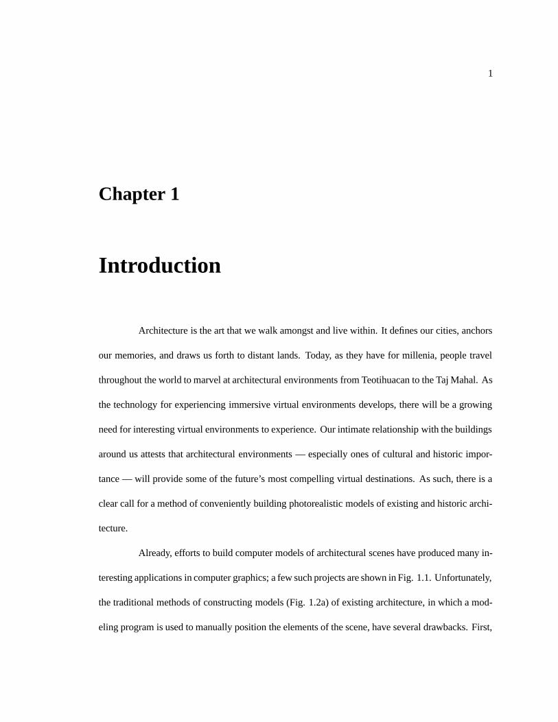
Figure 1.1: Three ambitious projects to model architecture with computers, each presented with arendering of the computer model and a photograph of the actual architecture. Top: Soda Hall Walk-thru Project [49, 15], University of California at Berkeley. Middle: Giza Plateau Modeling Project,University of Chicago. Bottom: Virtual Amiens Cathedral, Columbia University. Using traditionalmodeling techniques (Fig. 1.2a), each of these models required many person-months of effort tobuild, and although each project yielded enjoyable and useful renderings, the results are qualitativelyvery different from actual photographs of the architecture.

3

the process is extremely labor-intensive, typically involving surveying the site, locating and digitiz-

ing architectural plans (if available), or converting existing CAD data (again, if available). Second,

it is difficult to verify whether the resulting model is accurate. Most disappointing, though, is that

the renderings of the resulting models are noticeably computer-generated; even those that employ

liberal texture-mapping generally fail to resemble real photographs. As a result, it is very easy to

distinguish the computer renderings from the real photographs in Fig. 1.1.

Recently, creating models directly from photographs has received increased interest in both

computer vision and in computer graphics under the title of image-based modeling and rendering.

Since real images are used as input, such an image-based system (Fig. 1.2c) has an advantage in pro-

ducing photorealistic renderings as output. Some of the most promising of these systems ([24, 31, 27,

44, 37], see also Figs. 1.3 and 1.4) employ the computer vision technique of computational stereop-

sis to automatically determine the structure of the scene from the multiple photographs available. As

a consequence, however, these systems are only as strong as the underlying stereo algorithms. This

has caused problems because state-of-the-art stereo algorithms have a number of significant weak-

nesses; in particular, the photographs need to have similar viewpoints for reliable results to be ob-

tained. Because of this, current image-based techniques must use many closely spaced images, and

in some cases employ significant amounts of user input for each image pair to supervise the stereo

algorithm. In this framework, capturing the data for a realistically renderable model would require

an impractical number of closely spaced photographs, and deriving the depth from the photographs

could require an impractical amount of user input. These concessions to the weakness of stereo al-

gorithms would seem to bode poorly for creating large-scale, freely navigable virtual environments

from photographs.

4

ModelingProgram

model

RenderingAlgorithm

renderings

user input texture maps

(a) Geometry−Based

Model−BasedStereo

depth maps

Image Warping

renderings

user inputimages

basic model

Photogrammetric Modeling Program

(b) Hybrid Approach

Stereo Correspondence

Image Warping

renderings

(user input)

(c) Image−Based

depth maps

images

Figure 1.2: Schematic of how our hybrid approach combines geometry-based and image-based ap-proaches to modeling and rendering architecture from photographs. The geometry-based approachillustrated places the majority of the modeling task on the user, whereas the image-based approachplaces the majority of the task on the computer. Our method divides the modeling task into twostages, one that is interactive, and one that is automated. The dividing point we have chosen cap-italizes on the strengths of both the user and the computer to produce the best possible modelsand renderings using the fewest number of photographs. The dashed line in the geometry-basedschematic indicates that images may optionally be used in a modeling program as texture-maps. Thedashed line in the image-based schematic indicates that in some systems user input is used to ini-tialize the stereo correspondence algorithm. The dashed line in the hybrid schematic indicates thatview-dependent texture-mapping (as discussed in Chapter 6) can be used without performing stereocorrespondence.

5

Figure 1.3: The Immersion ’94 stereo image sequence capture rig, being operated by MichaelNaimark of Interval Research Corporation. Immersion ’94 was one project that attempted to cre-ate navigable, photorealistic virtual environments from photographic data. The stroller supports twoidentical 16mm movie cameras, and has an encoder on one wheel to measure the forward motion ofthe rig. The cameras are motor-driven and can be programmed to take pictures in synchrony at anydistance interval as the camera rolls forward. For much of the work done for the See Banff! project,the forward motion distance between acquired stereo pairs was one meter. Photo by Louis Psihoyos-Matrix reprinted from the July 11, 1994 issue of Fortune Magazine.

6

Figure 1.4: The Immersion ’94 image-based modeling and rendering (see Fig. 1.2c) project. The toptwo photos are a stereo pair (reversed for cross-eyed stereo viewing) taken with in Canada’s BanffNational. The film frame was overscanned to assist in image registration. The middle left photo is astereo disparity map produced by a parallel implementation of the Zabih-Woodfill stereo algorithm[59]. To its right the map has been processed using a left-right consistency check to invalidate regionswhere running stereo based on the left image and stereo based on the right image did not produceconsistent results. Below are two virtual views generated by casting each pixel out into space basedon its computed depth estimate, and reimaging the pixels into novel camera positions. On the left isthe result of virtually moving one meter forward, on the right is the result of virtually moving onemeter backward. Note the dark de-occluded areas produced by these virtual camera moves; theseareas were not seen in the original stereo pair. In the Immersion ’94 animations, these regions wereautomatically filled in from neighboring stereo pairs.

7

The research presented here aims to make the process of modeling architectural scenes

more convenient, more accurate, and more photorealistic than the methods currently available. To

do this, we have developed a new approach that draws on the strengths of both traditional geometry-

based and novel image-based methods, as illustrated in Fig. 1.2b. The result is that our approach

to modeling and rendering architecture requires only a sparse set of photographs and can produce

realistic renderings from arbitrary viewpoints. In our approach, a basic geometric model of the ar-

chitecture is recovered semi-automatically with an easy-to-use photogrammetric modeling system

(Chapter 5), novel views are created using view-dependent texture mapping (Chapter 6), and addi-

tional geometric detail can be recovered automatically through model-based stereo correspondence

(Chapter 7). The final images can be rendered with current image-based rendering techniques or

with traditional texture-mapping hardware. Because only photographs are required, our approach

to modeling architecture is neither invasive nor does it require architectural plans, CAD models, or

specialized instrumentation such as surveying equipment, GPS sensors or range scanners.

8

Chapter 2

Background and Related Work

The process of recovering 3D structure from 2D images has been a central endeavor within

computer vision, and the process of rendering such recovered structures is an emerging topic in com-

puter graphics. Although no general technique exists to derive models from images, several areas of

research have provided results that are applicable to the problem of modeling and rendering architec-

tural scenes. The particularly relevant areas reviewed here are: Camera Calibration, Structure from

Motion, Shape from Silhouette Contours, Stereo Correspondence, and Image-Based Rendering.

2.1 Camera calibration

Recovering 3D structure from images becomes a simpler problem when the images are

taken with calibrated cameras. For our purposes, a camera is said to be calibrated if the mapping

between image coordinates and directions relative to the camera center are known. However, the

position of the camera in space (i.e. its translation and rotation with respect to world coordinates)

is not necessarily known. An excellent presentation of the algebraic and matrix representations of

9

perspective cameras may be found in [13].

Considerable work has been done in both photogrammetry and computer vision to cali-

brate cameras and lenses for both their perspective intrinsic parameters and their distortion patterns.

Some successful methods include [52], [12], and [11]. While there has been recent progress in the

use of uncalibrated views for 3D reconstruction [14], this method does not consider non-perspective

camera distortion which prevents high-precision results for images taken through real lenses. In our

work, we have found camera calibration to be a straightforward process that considerably simpli-

fies the problem of 3D reconstruction. Chapter 4 provides a more detailed overview of the issues

involved in camera calibration and presents the camera calibration process used in this work.

2.2 Structure from motion

Given the 2D projection of a point in the world, its position in 3D space could be anywhere

on a ray extending out in a particular direction from the camera’s optical center. However, when

the projections of a sufficient number of points in the world are observed in multiple images from

different positions, it is mathematically possible to deduce the 3D locations of the points as well as

the positions of the original cameras, up to an unknown factor of scale.

This problem has been studied in the area of photogrammetry for the principal purpose of

producing topographic maps. In 1913, Kruppa [23] proved the fundamental result that given two

views of five distinct points, one could recover the rotation and translation between the two camera

positions as well as the 3D locations of the points (up to a scale factor). Since then, the problem’s

mathematical and algorithmic aspects have been explored starting from the fundamental work of

Ullman [54] and Longuet-Higgins [25], in the early 1980s. Faugeras’s book [13] overviews the state

10

of the art as of 1992. So far, a key realization has been that the recovery of structure is very sensitive

to noise in image measurements when the translation between the available camera positions is small.

Attention has turned to using more than two views with image stream methods such as

[50] or recursive approaches [2]. Tomasi and Kanade [50] (see Fig. 2.1) showed excellent results

for the case of orthographic cameras, but direct solutions for the perspective case remain elusive. In

general, linear algorithms for the problem fail to make use of all available information while nonlin-

ear optimization methods are prone to difficulties arising from local minima in the parameter space.

An alternative formulation of the problem by Taylor and Kriegman [47] (see Fig. 2.2) uses lines

rather than points as image measurements, but the previously stated concerns were shown to remain

largely valid. For purposes of computer graphics, there is yet another problem: the models recovered

by these algorithms consist of sparse point fields or individual line segments, which are not directly

renderable as solid 3D models.

In our approach, we exploit the fact that we are trying to recover geometric models of ar-

chitectural scenes, not arbitrary three-dimensional point sets. This enables us to include additional

constraints not typically available to structure from motion algorithms and to overcome the prob-

lems of numerical instability that plague such approaches. Our approach is demonstrated in a useful

interactive system for building architectural models from photographs (Chapter 5.)

2.3 Shape from silhouette contours

Some work has been done in both computer vision and computer graphics to recover the

shape of objects from their silhouette contours in multiple images. If the camera geometry is known

for each image, then each contour defines an infinite, cone-shaped region of space within which the

11

points.graph

Y

X-400.00

-380.00

-360.00

-340.00

-320.00

-300.00

-280.00

-260.00

-240.00

-220.00

-200.00

-180.00

-160.00

-140.00

-120.00

-100.00

200.00 300.00 400.00 500.00

Figure 2.1: Images from the 1992 Tomasi-Kanade structure from motion paper [50]. In this paper,feature points were automatically tracked in an image sequence of a model house rotating. By as-suming the camera was orthographic (which was approximated by using a telephoto lens), they wereable to solve for the 3D structure of the points using a linear factorization method. The above left pic-ture shows a picture from the original sequence, the above right picture shows a second image of themodel from above (not in the original sequence), and the plot below shows the 3D recovered pointsfrom the same camera angle as the above right picture. Although an elegant and fundamental result,this approach is not directly applicable to real-world scenes because real camera lenses (especiallythose typically used for architecture) are too wide-angle to be approximated as orthographic.

12

Figure 2.2: Images from the 1995 Taylor-Kriegman structure from motion paper [47]. In this work,structure from motion is recast in terms of line segments rather than points. A principal benefit of thisis that line features are often more easily located in architectural scenes than point features. Aboveare two of eight images of a block scene; edge correspondences among the images were provided tothe algorithm by the user. The algorithm then employed a nonlinear optimization technique to solvefor the 3D positions of the line segments as well as the original camera positions, show below. Thiswork used calibrated cameras, but allowed a full perspective model to be used in contrast to Tomasiand Kanade [50]. However, the optimization technique was prone to getting caught in local minimaunless good initial estimates of the camera orientations were provided. This work was extended tobecome the basis of the photogrammetric modeling method presented in Chapter 5.

13

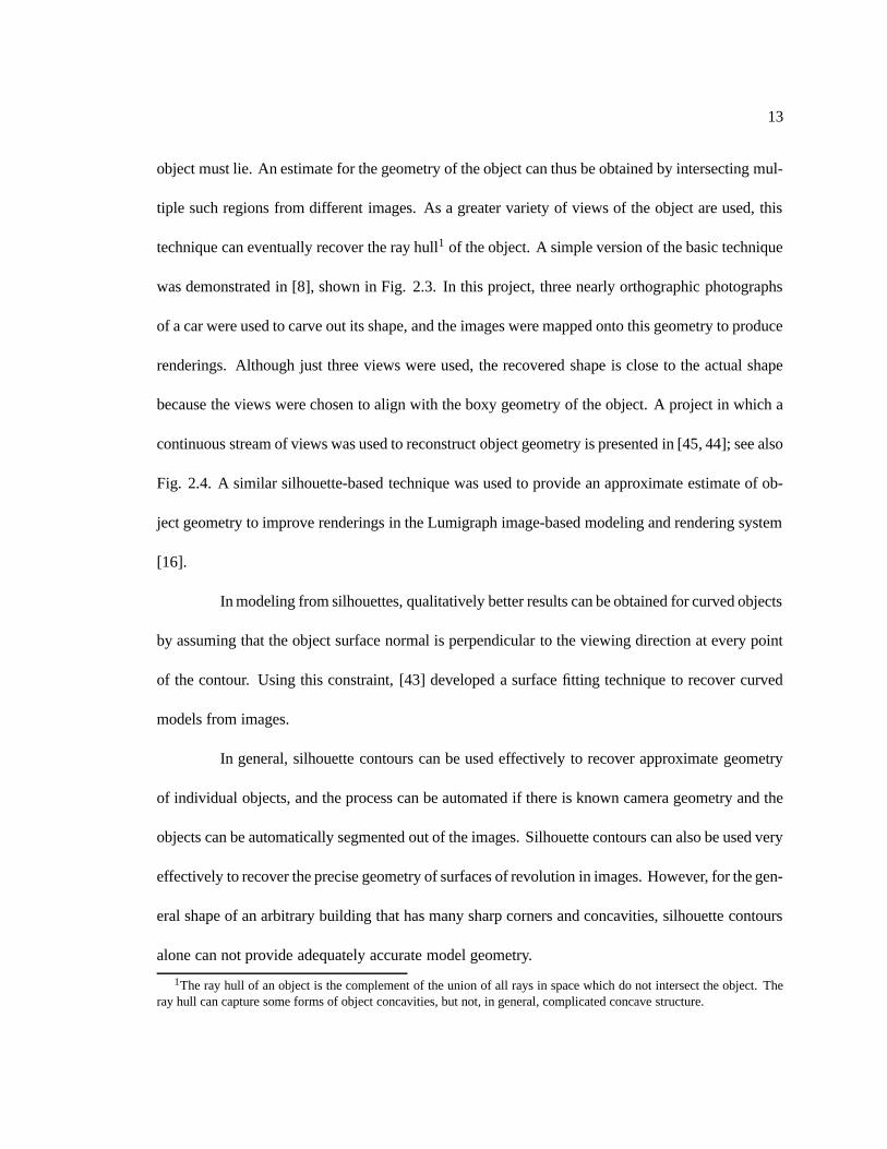
object must lie. An estimate for the geometry of the object can thus be obtained by intersecting mul-

tiple such regions from different images. As a greater variety of views of the object are used, this

technique can eventually recover the ray hull1 of the object. A simple version of the basic technique

was demonstrated in [8], shown in Fig. 2.3. In this project, three nearly orthographic photographs

of a car were used to carve out its shape, and the images were mapped onto this geometry to produce

renderings. Although just three views were used, the recovered shape is close to the actual shape

because the views were chosen to align with the boxy geometry of the object. A project in which a

continuous stream of views was used to reconstruct object geometry is presented in [45, 44]; see also

Fig. 2.4. A similar silhouette-based technique was used to provide an approximate estimate of ob-

ject geometry to improve renderings in the Lumigraph image-based modeling and rendering system

[16].

In modeling from silhouettes, qualitatively better results can be obtained for curved objects

by assuming that the object surface normal is perpendicular to the viewing direction at every point

of the contour. Using this constraint, [43] developed a surface fitting technique to recover curved

models from images.

In general, silhouette contours can be used effectively to recover approximate geometry

of individual objects, and the process can be automated if there is known camera geometry and the

objects can be automatically segmented out of the images. Silhouette contours can also be used very

effectively to recover the precise geometry of surfaces of revolution in images. However, for the gen-

eral shape of an arbitrary building that has many sharp corners and concavities, silhouette contours

alone can not provide adequately accurate model geometry.

1The ray hull of an object is the complement of the union of all rays in space which do not intersect the object. Theray hull can capture some forms of object concavities, but not, in general, complicated concave structure.

14

Figure 2.3: Images from the 1991 Chevette Modeling project [8]. The top three images show pic-tures of the 1980 Chevette photographed with a 210mm lens from the top, side, and front. TheChevette was semi-automatically segmented from each image, and these images were then regis-tered with each other approximating the projection as orthographic. The registered photographs areshown placed in proper relation to each other on the faces of a rectangular box in the center of thefigure. The shape of the car is then carved out from the box volume by perpendicularly sweepingeach of the three silhouettes like a cookie-cutter through the box volume. The recovered volume(shown inside the box) is then textured-mapped by projecting the original photographs onto it. Thebottom of the figure shows a sampling of frames from a synthetic animation of the car flying acrossthe screen. Although (and perhaps because) the final model has flaws resulting from specularities,missing concavities, and imperfect image registration, it unequivocally evokes an uncanny sense ofthe actual vehicle.

15

Figure 2.4: Images from a silhouette modeling project by Rick Szeliski [45, 44]. The cup was video-taped on a rotating platform (left), and the extracted contours from this image sequence were usedto automatically recover the shape of the cup (right).

Although not adequate for general building shapes, silhouette contours could be useful in

recovering the approximate shapes of trees, bushes, and topiary in architectural scenes. Techniques

such as those presented in [36] could then be used to synthesize detailed plant geometry to con-

form to the shape and type of the original flora. This technique would seem to hold considerably

more promise for practically recovering plant structure than trying to reconstruct the position and

coloration of each individual leaf and branch of every tree in the scene.

2.4 Stereo correspondence

The geometrical theory of structure from motion assumes that one is able to solve the cor-

respondence problem, which is to identify the points in two or more images that are projections of

the same point in the world. In humans, corresponding points in the two slightly differing images on

the retinas are determined by the visual cortex in the process called binocular stereopsis. Two terms

used in reference to stereo are baseline and disparity. The baseline of a stereo pair is the distance

16

between the camera locations of the two images. Disparity refers to the difference in image location

between corresponding features in the two images, which is projectively related to the depth of the

feature in the scene.

Years of research (e.g. [3, 10, 17, 22, 26, 32, 35]) have shown that determining stereo cor-

respondences by computer is difficult problem. In general, current methods are successful only when

the images are similar in appearance, as in the case of human vision, which is usually obtained by

using cameras that are closely spaced relative to the objects in the scene. As the distance between

the cameras (often called the baseline) increases, surfaces in the images exhibit different degrees

of foreshortening, different patterns of occlusion, and large disparities in their locations in the two

images, all of which makes it much more difficult for the computer to determine correct stereo cor-

respondences. To be more specific, the major sources of difficulty include:

1. Foreshortening. Surfaces in the scene viewed from different positions will be foreshortened

differently in the images, causing the image neighborhoods of corresponding pixels to appear

dissimilar. Such dissimilarity can confound stereo algorithms that use local similarity metrics

to determine correspondences.

2. Occlusions. Depth discontinuities in the world can create half-occluded regions in an image

pair, which also poses problems for local similarity metrics.

3. Lack of Texture. Where there is an absence of image intensity features it is difficult for a

stereo algorithm to correctly find the correct match for a particular point, since many point

neighborhoods will be similar in appearance.

Unfortunately, the alternative of improving stereo correspondence by using images taken

from nearby locations has the disadvantage that computing depth becomes very sensitive to noise in

17

image measurements. Since depth is computed by taking the inverse of disparity, image pairs with

small disparities tend to give rise to noisy depth estimates. Geometrically, depth is computed by

triangulating the position of a matched point from its imaged position in the two cameras. When

the cameras are placed close together, this triangle becomes very narrow, and the distance to its apex

becomes very sensitive to the angles at its base. Noisy depth estimates mean that novel views will be-

come visually unconvincing very quickly as the virtual camera moves away from the original view-

point.

Thus, computing scene structure from stereo leaves us with a conundrum: image pairs with

narrow baselines (relative to the distance of objects in the scene) are similar in appearance and make

it possible to automatically compute stereo correspondences, but give noisy depth estimates. Im-

age pairs with wide baselines can give very accurate depth localization for matched points, but the

images usually exhibit large disparities, significant regions of occlusion, and different forms of fore-

shortening which makes it very difficult to automatically determine correspondences.

In the work presented in this thesis, we address this conundrum by showing that having

an approximate model of the photographed scene can be used to robustly determine stereo corre-

spondences from images taken from widely varying viewpoints. Specifically, the model enables us

to warp the images to eliminate unequal foreshortening and to predict major instances of occlusion

before trying to find correspondences. This new form of stereo is called model-based stereo and is

presented in Chapter 7.

18

2.5 Range scanning

Instead of the anthropomorphic approach of using multiple images to reconstruct scene

structure, an alternative technique is to use range imaging sensors [5] to directly measure depth to

various points in the scene. Range imaging sensors determine depth either by triangulating the po-

sition of a projected laser stripe, or by measuring the time of flight of a directional laser pulse. Early

versions of these sensors were slow, cumbersome and expensive. Although many improvements

have been made, so far the most convincing demonstrations of the technology have been on human-

scale objects and not on architectural scenes. Algorithms for combining multiple range images from

different viewpoints have been developed both in computer vision [58, 42, 40] and in computer

graphics [21, 53], see also Fig. 2.5. In many ways, range image based techniques and photographic

techniques are complementary and have their relative advantages and disadvantages. Some advan-

tages of modeling from photographic images are that (a) still cameras are inexpensive and widely

available and (b) for some architecture that no longer exists all that is available are photographs.

Furthermore, range images alone are insufficient for producing renderings of a scene; photometric

information from photographs is also necessary.

2.6 Image-based modeling and rendering

In an image-based rendering system, the model consists of a set of images of a scene and

their corresponding depth maps. When the depth of every point in an image is known, the image can

be re-rendered from any nearby point of view by projecting the pixels of the image to their proper 3D

locations and reprojecting them onto a new image plane. Thus, a new image of the scene is created by

warping the images according to their depth maps. A principal attraction of image-based rendering is

19

(a) (b)

(c) (d)

Figure 2.5: Several models constructed from triangulation-based laser range scanning techniques.(a) A model of a person’s head scanned using a commercially available Cyberware laser range scan-ner, using a cylindrical scan. (b) A texture-mapped version of this model, using imagery acquiredby the same video camera used to detect the laser stripe. (c) A more complex geometry assembledby zippering together several triangle meshes obtained from separate linear range scans of a smallobject from [53]. (d) An even more complex geometry acquired from over sixty range scans usingthe volumetric recovery method in [7].

20

that it offers a method of rendering arbitrarily complex scenes with a constant amount of computation

required per pixel. Using this property, [57] demonstrated how regularly spaced synthetic images

(with their computed depth maps) could be warped and composited in real time to produce a virtual

environment.

In [31], shown in Fig. 1.4, stereo photographs with a baseline of eight inches were taken

every meter along a trail in a forest. Depth was extracted from each stereo pair using a census stereo

algorithm [59]. Novel views were produced by supersampled z-buffered forward pixel splatting

based on the stereo depth estimate of each pixel. ([24] describes a different rendering approach that

implicitly triangulated the depth maps.) By manually determining relative camera pose between suc-

cessive stereo pairs, it was possible to optically combine rerenderings from neighboring stereo pairs

to fill in missing texture information. The project was able to produce very realistic synthetic views

looking forward along the trail from any position within a meter of the original camera path, which

was adequate for producing a realistic virtual experience of walking down the trail. Thus, for mostly

linear environments such as a forest trail, this method of capture and rendering seems promising.

More recently, [27] presented a real-time image-based rendering system that used panoramic

photographs with depth computed, in part, from stereo correspondence. One finding of the paper was

that extracting reliable depth estimates from stereo is “very difficult”. The method was nonetheless

able to obtain acceptable results for nearby views using user input to aid the stereo depth recovery:

the correspondence map for each image pair was seeded with 100 to 500 user-supplied point cor-

respondences and also post-processed. Even with user assistance, the images used still had to be

closely spaced; the largest baseline described in the paper was five feet.

The requirement that samples be close together is a serious limitation to generating a freely

21

navigable virtual environment. Covering the size of just one city block would require thousands of

panoramic images spaced five feet apart. Clearly, acquiring so many photographs is impractical.

Moreover, even a dense lattice of ground-based photographs would only allow renderings to be gen-

erated from within a few feet of the original camera level, precluding any virtual fly-bys of the scene.

Extending the dense lattice of photographs into three dimensions would clearly make the acquisition

process even more difficult.

The modeling and rendering approach described in this thesis takes advantage of the struc-

ture in architectural scenes so that only a sparse set of photographs can be used to recover both the

geometry and the appearance of an architectural scene. For example, our approach has yielded a

virtual fly-around of a building from just twelve photographs (Fig. 5.14).

Some research done concurrently with the work presented in this thesis [4] also shows that

taking advantage of architectural constraints can simplify image-based scene modeling. This work

specifically explored the constraints associated with the cases of parallel and coplanar edge segments.

None of the work discussed so far has presented how to use intensity information coming

from multiple photographs of a scene, taken from arbitrary locations, to render recovered geome-

try. The view-dependent texture mapping work (Chapter 6) presented in this thesis presents such a

method.

Lastly, our model-based stereo algorithm (Chapter 7) presents an approach to robustly ex-

tracting detailed scene information from widely-spaced views by exploiting an approximate model

of the scene.

22

Chapter 3

Overview

In this paper we present three new modeling and rendering techniques: photogrammet-

ric modeling, view-dependent texture mapping, and model-based stereo. We show how these tech-

niques can be used in conjunction to yield a convenient, accurate, and photorealistic method of mod-

eling and rendering architecture from photographs. In our approach, the photogrammetric modeling

program is used to create a basic volumetric model of the scene, which is then used to constrain

stereo matching. Our rendering method composites information from multiple images with view-

dependent texture-mapping. Our approach is successful because it splits the task of modeling from

images into tasks which are easily accomplished by a person (but not a computer algorithm), and

tasks which are easily performed by a computer algorithm (but not a person).

In Chapter 4, we discuss camera calibration from the standpoint of reconstructing archi-

tectural scenes from photographs. We present the method of camera calibration used in the work

presented in this thesis, in which radial distortion is estimated separately from the perspective cam-

era geometry. We also discuss methods of using uncalibrated views, which are quite often necessary

23

to work with when using historic photographs.

In Chapter 5, we present our photogrammetric modeling method. In essence, we have

recast the structure from motion problem not as the recovery of individual point coordinates, but

as the recovery of the parameters of a constrained hierarchy of parametric primitives. The result is

that accurate architectural models can be recovered robustly from just a few photographs and with a

minimal number of user-supplied correspondences.

In Chapter 6, we present view-dependent texture mapping, and show how it can be used

to realistically render the recovered model. Unlike traditional texture-mapping, in which a single

static image is used to color in each face of the model, view-dependent texture mapping interpolates

between the available photographs of the scene depending on the user’s point of view. This results

in more lifelike animations that better capture surface specularities and unmodeled geometric detail.

In Chapter 7, we present model-based stereo, which is used to automatically refine a basic

model of a photographed scene. This technique can be used to recover the structure of architectural

ornamentation that would be difficult to recover with photogrammetric modeling. In particular, we

show that projecting pairs of images onto an initial approximate model allows conventional stereo

techniques to robustly recover very accurate depth measurements from images with widely varying

viewpoints.

Lastly, in Chapter 8, we present Rouen Revisited, an interactive art installation that repre-

sents an application of all the techniques developed in this thesis. This work, developed in collab-

oration with Interval Research Corporation, involved modeling the detailed Gothic architecture of

the West facade of the Rouen Cathedral, and then rendering it from any angle, at any time of day,

in any weather, and either as it stands today, as it stood one hundred years ago, or as the French

24

Impressionist Claude Monet might have painted it.

As we mentioned, our approach is successful not only because it synthesizes these geometry-

based and image-based techniques, but because it divides the task of modeling from images into

sub-tasks which are easily accomplished by a person (but not a computer algorithm), and sub-tasks

which are easily performed by a computer algorithm (but not a person.) The correspondences for the

reconstruction of the coarse model of the system are provided by the user in an interactive way; for

this purpose we have designed and implemented Facade (Chapter 5), a photogrammetric modeling

system that makes this task quick and simple. Our algorithm is designed so that the correspondences

the user must provide are few in number per image. By design, the high-level model recovered by

the system is precisely the sort of scene information that would be difficult for a computer algorithm

to discover automatically. The geometric detail recovery is performed by an automated stereo corre-

spondence algorithm (Chapter 7), which has been made feasible and robust by the pre-warping step

provided by the coarse geometric model. In this case, corresponding points must be computed for a

dense sampling of image pixels, a job too tedious to assign to a human, but feasible for a computer

to perform using model-based stereo.

25

Chapter 4

Camera Calibration

Recovering 3D structure from images becomes a simpler problem when the images are

taken with calibrated cameras. For our purposes, a camera is said to be calibrated if the mapping

between image coordinates and directions relative to the camera center are known. However, the

position of the camera in space (i.e. its translation and rotation with respect to world coordinates) is

not necessarily known.

4.1 The perspective model

For an ideal pinhole camera delivering a true perspective image, this mapping can be char-

acterized completely by just five numbers, called the intrinsic parameters of the camera. In contrast,

a camera’s extrinsic parameters represent its location and rotation in space. The five intrinsic camera

parameters are:

1. The x-coordinate of the the center of projection, in pixels (u0)

2. The y-coordinate of the the center of projection, in pixels (v0)

26

3. The focal length, in pixels ( f )

4. The aspect ratio (a)

5. The angle between the optical axes (c)

An excellent presentation of the algebraic and matrix representations of perspective cam-

eras may be found in [13].

The calibration of real cameras is often approximated with such a five-parameter mapping,

though rarely is such an approximation accurate to the pixel. The next section will discuss how real

images differ from true perspective and a procedure for correcting for the difference. While several

methods have been presented to determine the the intrinsic parameters of a camera from images it

has taken, approximate values for these parameters can often be assumed a priori.

For most images taken with standard lenses, the center of projection is at or near the co-

ordinate center of the image. However, small but significant shifts are often introduced in the image

recording or digitizing process. Such an image shift has the most impact on camera calibration for

lenses with shorter focal lengths. Images that have been cropped may also have centers of projection

far from the image center.

Old-fashioned bellows cameras, and modern cameras with tilt-shift lenses, can be used to

place the center of projection far from the center of the image. This is most often used in architectural

photography, when the photographer places the film plane vertically and shifts the lens upward until

the top of the building projects onto the film area. The result is that vertical lines remain parallel

rather than converging toward the top of the picture, which would happen if the photographer had

simply rotated the camera upwards. To extract useful geometric information out of such images, it

is necessary to compute the center of projection.

27

The focal length of the camera in pixels can be estimated by dividing the marked focal

length of the camera lens by the width of the image on the imaging surface (the film or CCD array),

and then multiplying by the width of the final image in pixels. For example, the images taken with

a 35mm film camera are 36mm wide and 24mm high1. Thus an image taken with a 50mm lens and

digitized at 768 by 512 pixels would have an approximate focal length of (50=36)� 768 = 1067

pixels. The reason this is approximate is that the digitization process typically crops out some of the

original image, which increases the observed focal length slightly. Of course, zoom lenses are vari-

able in focal length so this procedure may only be applied if the lens was known to be fully extended

or retracted.

It should be noted that most prime2 lenses actually change in focal length depending on the

distance at which they are focussed. This means that images taken with the same lens on the same

camera may exhibit different focal lengths, and thus need separate camera calibrations. The easiest

solution to this problem is to fix the focus of the lens at infinity and use a small enough aperture small

to image the closest objects in the scene in focus. Another solution is to use telecentric lenses, whose

focal length is independent of focus. A procedure for converting certain regular lenses to telecentric

ones is presented in [55].

The aspect ratio for images taken with real cameras with radially symmetric lens elements

is 1.0, although recording and digitizing processes can change this. The Kodak PhotoCD process for

digitizing film maintains a unit aspect ratio. Some motion-picture cameras used to film wide screen

features use non-radially symmetric optics to squeeze a wide image into a relatively narrow frame;

these images are then expanded during projection. In this case, the aspect ratio is closer to 2.0.

135mm refers to the height of the entire film strip, including the sprocket holes2A prime lens is a lens with a fixed focal length, as opposed to a zoom lens, which is variable in focal length.

28

Finally, for all practical cases of images acquired with real cameras and digitized with stan-

dard equipment, the angle between the optical axes is 90 degrees.

4.2 How real cameras deviate from the pinhole model

Real cameras deviate from the pinhole model in several respects. First, in order to col-

lect enough light to expose the film, light is gathered across the entire surface of the lens. The most

noticeable effect of this is that only a particular surface in space, called the focal plane3, will be in

perfect focus. In terms of camera calibration, each image point corresponds not to a single ray from

the camera center, but to a set of rays from across the front of the lens all converging on a particular

point on the focal plane. Fortunately, the effects of this area sampling can be made negligible by

using a suitably small camera aperture.

The second, and most significant effect, is lens distortion. Because of various constraints

in the lens manufacturing process, straight lines in the world imaged through real lenses generally

become somewhat curved on the image plane. However, since each lens element is radially symmet-

ric, and the elements are typically placed with high precision on the same optical axis, this distortion

is almost always radially symmetric, and is referred to as radial lens distortion. Radial distortion

that causes the image to bulge toward the center is called barrel distortion, and distortion that causes

the image to shrink toward the center is called pincushion distortion. Some lenses actually exhibit

both properties at different scales.

To correct for radial distortion, one needs to recover the center of the distortion (cx;cy),

usually consistent with the center of projection of the image, and a radial transformation function

3Although called the focal plane, this surface is generally slightly curved for real lenses

29

that remaps radii from the center such that straight lines stay straight:

r0 = F(r) (4.1)

Usually, the radial distortion function is modeled as r multiplied by an even polynomial of

the form:

F(r) = r(1+ k1r2 + k2r4 + :::) (4.2)

The multiplying polynomial is even in order to ensure that the distortion is C∞ continu-

ous at the center of distortion, and the first coefficient is chosen to be unity so that the original and

undistorted images agree in scale at the center of distortion. These coefficients can be determined

by measuring the curvature of putatively straight lines in images. Such a method will be presented

in the next section.

The distortion patterns of cameras with imperfectly ground or imperfectly aligned optics

may not be radially symmetric, in which case it is necessary to perform a more general distortion

correction.

Another deviation from the pinhole model is that in film cameras the film plane can deviate

significantly from being a true plane. The plate at the back of the camera may not be perfectly flat,

or the film may not lie firmly against it. Also, many film digitization methods do not ensure that the

film is perfectly flat during the scanning process. These effects, which we collectively refer to as film

flop, cause subtle deformations in the image. Since some of the deformations are different for each

photograph, they cannot be corrected for beforehand through camera calibration. Digitial cameras,

which have precisely flat and rectilinear imaging arrays, are generally not susceptible to this sort of

30

distortion.

A final, and particularly insidious deviation from the pinhole camera model is that the im-

aged rays do not necessarily intersect at a point. As a result, there need not be a mathematically

precise principal point, or nodal point for a real lens, as illustrated in Fig. 4.1. As a result, it is im-

possible to say with complete accuracy that a particular image was taken from a particular location

in space; each pixel must be treated as its own separate ray. Although this effect is most noticeable in

extreme wide-angle lenses, the locus of convergence is almost always small enough to be treated as

a point, especially when the objects being imaged are large with respect to the locus of convergence.

film

pla

ne

film

pla

ne

incoming rays

principalpoint

Pinhole Camera Lens Camera

locus ofconvergence

incoming rays

Figure 4.1: In a pinhole camera, all the imaged rays must pass though the pinhole, which effectivelybecomes the mathematical location of the camera. In a real camera with a real lens, the imaged raysneed not all intersect at a point. Although this effect is usually insignificant, to treat it correctly wouldcomplicate the problems of camera calibration and 3D reconstruction considerably.

Considerable work has been done in both photogrammetry and computer vision to cali-

brate cameras and lenses for both their perspective intrinsic parameters and their distortion patterns.

Some successful methods include [52], [12], and [11]. While there has been recent progress in the

use of uncalibrated views for 3D reconstruction [14], this method does not consider non-perspective

camera distortion which prevents high-precision results for images taken through real lenses. In our

work, we have found camera calibration to be a straightforward process that considerably simplifies

the problem of 3D reconstruction. The next section presents the camera calibration process used for

31

our project.

4.3 Our calibration method

Our calibration method uses two calibration objects. For each camera/lens configuration

used in the reconstruction project, a few photographs of each calibration object are taken. The first

calibration object (Fig. 4.2) is a flat checkerboard pattern, and is used to recover the pattern of radial

distortion from the images. The second object (Fig. 4.8) is two planes with rectangular patterns set

at a 90 degree angle to each other, and is used to recover the intrinsic perspective parameters of the

camera.

4.4 Determining the radial distortion coefficients

The first part of the calibration process is to determine an image coordinate remapping that

causes images taken by the camera to be true perspective images, that is, straight lines in the world

project as straight lines in the image. The procedure makes use of one or several images with many

known straight lines in it. Architectural scenes are usually a rich source of straight lines, but for most

of the work in this thesis we used pictures of the checkerboard pattern shown below (Fig. 4.2) to

determine the radial lens distortion. The checkerboard pattern is a natural choice since straight lines

with easily localized endpoints and interior points can be found in several orientations (horizontal,

vertical, and various diagonals) throughout the image plane.

The checkerboard pattern also has the desirable property that its corners are localizable

independent of the linearity of the image response. That is, applying a nonlinear monotonic function

to the intensity values of the checkerboard image, such as gamma correction, does not affect corner

32

localization. As a counterexample, this is not the case for the corners of a white square on a black

background. If the image is blurred somewhat, changing the image gamma will cause the square to

shrink or enlarge, which will affect corner localization.

Figure 4.2: Original image of a calibration checkerboard pattern, taken with a Canon 24mm EF lens.The straight lines in several orientations throughout this image are used to determine the pattern ofradial lens distortion. The letter “P” in the center is used to record the orientation of the grid withrespect to the camera.

The pattern in Fig. 4.2 was photographed with a 24mm lens on a Canon EOS Elan camera.

Since this lens, like most, changes its internal configuration depending on the distance it is focussed

at, it is possible that its pattern of radial distortion could be different depending on where it is fo-

cussed. Thus, care was taken to focus the lens at infinity and to reduce the aperture until the image

was adequately sharp. Clearly, this procedure works only when the calibration object is far enough

from the camera to be brought into focus via a small aperture. Since wide-angle lenses generally

have large depths of field, this was not a problem for the 24mm lens with a 50cm high calibration

grid. However, the depth of field of a 200mm lens was too shallow to focus the object even when

fully stopped down — a larger calibration object, placed further away, was called for.

33

The pattern of radial distortion in Fig. 4.2 may be too subtle to be seen directly, so I have

developed a procedure for more easily visualizing lens distortion in checkerboard test images. First,

a simple Sobel edge detector is run on the image to produce the image shown in 4.3.

Figure 4.3: The edges of the checkerboard pattern found by using a simple Sobel edge detector.(Shown in reverse video)

The pattern of distortion can now be made evident to a human observer by shrinking this

edge image in either the horizontal or the vertical direction by an extreme amount. Fig. 4.4 shows

this edge image shrunk in both the vertical and horizontal directions by a factor of 50. In the case

of this 24mm lens, we can see that lines passing through the center of the image stay straight, as do

the vertical lines at the extreme left and right of the image. Lines which lie at intermediate distances

from the center of the image are bowed. The bottom image, resulting from shrinking the image in

the horizontal direction and rotating by 90 degrees, shows that this bowing is actually not convex.

We will see this represented in the radial distortion coefficients as a positive k1 and a negative k2.

The choice of the checkerboard pattern makes it possible to automatically localizing image

points. Image points can be easily localized by first convolving the image with the filter in Table

34

Figure 4.4: The results of changing the aspect ratio of the image in Fig. 4.3 by a factor of 50 in boththe horizontal (top) and vertical (bottom, rotated 90 degrees) directions. This extreme change inaspect ratio makes it possible for a human observer to readily examine the pattern of lens distortion.

-1 -1 -1 0 1 1 1-1 -1 -1 0 1 1 1-1 -1 -1 0 1 1 10 0 0 0 0 0 01 1 1 0 -1 -1 -11 1 1 0 -1 -1 -11 1 1 0 -1 -1 -1

Table 4.1: A 7�7 convolution filter that detects corners of the checkerboard pattern.

4.4. Since this filter itself resembles a checkerboard pattern, it gives a strong response (positive or

negative, depending on which type of corner) when centered over a checkerboard corner. Taking

the absolute value of the filter output produces an image where the checkerboard corners appear as

white dots, as in Fig. 4.5.

Localizing a particular checkerboard corner after the filter convolution is easily accom-

plished by locating the point of maximum filter response. Sub-pixel accuracy can be obtained by

examining the filter responses at pixels neighboring the pixel of maximum response, fitting these re-

sponses with an upside-down paraboloid, and calculating the location of the global maximum of the

paraboloid.

The localized checkerboard corners provide many sets of points which are collinear in the

world. In fact, these sets of points can be found in many orientations, including horizontal, verti-

cal, and diagonal. However, because of lens distortion, these points will in general not be precisely

collinear in the image. For any such set of points, one can quantify its deviation from linear by fitting

35

Figure 4.5: The results of convolving the checkerboard image with the filter in Table 4.4, and takingthe absolute value of the filter outputs. Both corners that are white at the upper-left and black at theupper left become easily detectable dots. (Shown in reverse video)

a line to the set of points in a least squares sense and summing the squared distances of the points

from the line. In the distortion correction method described here, triples of world-collinear points are

used to measure the lens distortion. The amount of error contributed by a triple of points is shown

in Fig. 4.6.

p0p1

p2

d

Figure 4.6: The distortion error function for a single line of three world-collinear points. The error isthe distance d between the middle point p1 from the line connecting the endpoints p0 and p2. Thiserror is summed over many triples of world-collinear points to form an objective function, which isthen optimized to determine the radial distortion coefficients of the lens.

The errors for many triples of world-collinear points throughout the image are summed to

36

produce an objective function Od that measures the extent to which the lens deviates from the true

pinhole model. Applying a radial distortion pattern with parameters (cx;cy;k1;k2;k3) to the coordi-

nates of the localized point triples will change the value of Od, and when the best values for these

parameters are chosen, the objective function will be at its global minimum. Thus, the radial distor-

tion parameters can be computed by finding the minimum of Od. For this work the minimum was

found for a variety of lenses using the fminu function of the MATLAB numerical analysis package.

For the particular 1536�1024 image in 4.2, the parameters computed were:

cx = 770:5 (4.3)

cy = 506:0 (4.4)

k1 = 9:46804�10�8 (4.5)

k2 =�7:19742�10�14 (4.6)

Note that the center of distortion, (770:5;506:0) is near but not at the center of the image

(768;512). The fact that the two distortion coefficients k1 and k2 are opposite in sign models the

wavy, non-convex nature of some of the distorted lines seen in Fig. 4.4.

Once the distortion parameters are solved for, it is possible to undistort any image taken

with the same lens as the calibration images so that straight lines in the world image to straight lines

on the image plane. In this work, the undistortion process could be performed without loss of image

quality because the PhotoCD images were available in higher resolutions than those that were used in

the reconstruction software. Specifically, images at 1536�1024 pixels were undistorted using sub-

pixel bilinear interpolation and then filtered down to 768�512 pixels for use in the software, making

any loss of image quality due to resampling negligible. Note that performing this resampling requires

37

the construction of a backward coordinate lookup function from undistorted to distorted image co-

ordinates, which requires finding the inverse of the distortion polynomial in Equation 4.2. Since this

is difficult to perform analytically, in this work the inverse function was inverted numercaly.

As a test of the radial distortion calibration, one can undistort the calibration images them-

selves and see if the original straight lines become straight. Fig. 4.7 shows the results of undistorting

the original checkerboard image, and just below with edge detection and shrinking as in Figs. 4.3

and 4.4 to better reveal the straightness of the lines in the image.

Figure 4.7: Top: The results of solving for the radial distortion parameters of the 24mm lens basedon the points in Fig. 4.5, and unwarping the original grid image (Fig. 4.2) and running edge detectionon it. Bottom: The two bottom images, scaled by a factor of fifty in either direction, help verify thatwith the distortion correction, the lines are now straight. Compare to the curved lines in 4.4. Notethat the lines are not parallel; this is because the camera’s film plane was not placed exactly parallelto the plane of the grid. It is a strength of this method that such alignment is not necessary.

38

4.5 Determining the intrinsic parameters

Once the distortion pattern of a lens is known, we can use any image taken with that lens,

undistort it, and then have an image in which straight lines in the world will project to straight lines

in the image. As a result, the projection is now a true perspective projection, and it becomes possible

to characterize the lens in terms of its five intrinsic parameters (see Sec. 4.1).

For this project, we used a calibration process provided to us by Q.T. Luong [11]. In this

method, an image of a calibration object, shown in Fig. 4.8, is used to determine the intrinsic param-

eters. The computer knows the geometry of the model a priori, and since the model has sufficient 3D

structure, the computer can solve for the eleven-degree-of-freedom projection matrix that would give

rise to the image of the object. This matrix is then factored into the camera’s six extrinsic parame-

ters (translation and rotation of the camera relative to the object) and the five intrinsic parameters. In

practice, solving for the 4�3 projection matrix is done with a nonlinear optimization over its twelve

elements, and the process is given an initial estimate by the user.

Figure 4.8: Q.T. Luong’s calibration object, photographed at several orientations. The three pho-tographs of the object were used to recover the intrinsic parameters of the 24mm Canon EOS lensused to take the photographs. Before solving for the perspective projection parameters, the lens’radial distortion pattern was modeled separately using a checkerboard grid object (Fig. 4.2). As aresult, the lens calibration was far more accurate.

A more reliable estimate of the intrinsic camera parameters can be obtained by photograph-

ing the grid in several orientations with respect to each camera lens. Fig. 4.8 shows the object at

39

Before undistorting αu αv f aImage 1 559.603 557.444 389.686 1.019Image 2 548.419 547.001 400.529 1.056Image 3 555.370 551.893 383.531 1.073

After undistorting αu αv f aImage 1 531.607 530.964 387.109 1.017Image 2 529.178 528.188 387.173 1.018Image 3 530.988 529.954 387.930 1.029

Table 4.2: Computed intrinsic parameters for the three images of the calibration object in Fig. 4.8,with and without first solving and correcting for radial distortion. The fifth intrinsic parameter, theangle between the optical axes c, is not shown since it was negligibly different from ninety degrees.Note that the parameters are far more consistent with each other after correcting for radial distortion.Without the correction, the distortion introduces different errors into the calibration depending on theposition and orientation of the calibration object.

three different orientations with a particular 24mm lens. The intrinsic parameters were solved for

separately using each orientation, and these results were averaged to obtain the final estimate of the

parameters. The importance of first solving for the pattern of radial distortion was well illustrated

by an attempt to solve for the intrinsic parameters in the three separate images with and without dis-

tortion correction. Table 4.5 shows that the parameters derived from the three images were suitably

consistent with each other using distortion correction, and much less consistent without distortion

correction.

4.6 Working with uncalibrated images

While camera calibration is a simple and straightforward process that can simplify pho-

togrammetry considerably, some very attractive applications require the use of images taken with un-

calibrated cameras. (One such application is described in Chapter 8). Specifically, photographs exist

for many architectural scenes that have since been modified or destroyed. As an example, Berkeley’s

original campus designed by John Galen Howard in the late 1800’s featured half a dozen Victorian

40

brick structures, of which only South Hall remains. Nonetheless, hundreds of photos of North Hall,

Bacon Hall, and the rest of the original campus sit in the university’s archives (for an example, see

Fig. 4.9). To use these photographs, it is necessary to determine the camera parameters without pic-

tures of calibration objects.

Figure 4.9: The original Berkeley campus in the late 1800’s, looking to the East. Of the four build-ings, only South Hall on the right remains. The ability to reconstruct buildings long since destroyedis a principal attraction of modeling architecture from photographs.

Fortunately, for architectural scenes, the buildings themselves are often serviceable cali-

bration objects. Straight lines, prevalent in architecture, can be used to determine radial lens dis-

tortion directly from the original photographs using the same method presented in Sec. 4.4. Shawn

Becker [4] presents another method of solving for radial distortion by observing sets of parallel lines,

also prevalent in architectural images.

The perspective intrinsic camera parameters can often be determined directly by observing

the vanishing points of orthogonal sets of parallel lines. If the aspect ratio a can be assumed to be

one, and the angle between the optical axes can be assumed to 90 degrees, then the remaining cam-

era parameters (center of projection and focal length) can be determined by observing the vanishing

points of three mutually orthogonal sets of lines. Geometrically, one simply needs to construct the

triangle connecting the three vanishing points on the image plane, and then intersect the image with

the corner of a cube such that each side of this triangle is coincident with a different face of the cube.

41

The corner of the cube will then be at the original camera center; the center of projection is obtained

by dropping a perpendicular from the camera center to the image plane, and the focal length is the

length of this perpendicular. Another discussion of related calibration techniques may be found in

[51].

Often, photos of since-demolished or modified buildings show structures that still exist,

as in Fig. 4.9. In these cases, it is possible to acquire calibrated images to reconstruct the existing

architecture and then use these dimensions to recover the historic camera parameters. This technique,

in conjunction with the vanishing-point technique just described, was used to determine the intrinsic

camera parameters of the historic photographs used in the Rouen Revisited art installation (Sec. 8).

Some researchers [14] have explored the mathematical theory and performed experiments

to recover structure from uncalibrated views. As mentioned, these techniques are not able to directly

solve for radial distortion effects, and only recover structure up to an arbitrary projective transfor-

mation. Nonetheless, the techniques show that recovering some intrinsic camera information from

uncalibrated views can be done implicitly as part of the structure recovery process.

Section 5 will describe our optimization technique for recovering building structure and

extrinsic camera parameters from calibrated photographs. A final method of making use of uncali-

brated views would be to include the intrinsic camera parameters, as well as the radial distortion co-

efficients, in the optimization. Further work would need to be done to use uncalibrated views in our

current initial estimate generation method. Also, one should be wary of the possibilities of obtain-

ing ill-conditioned or ambiguous solutions in situations where unconstrained descriptions of camera

geometry need to be obtained at the same time as the structure of the scene.

42

Chapter 5

Photogrammetric Modeling

This chapter presents our photogrammetric modeling method, in which the computer de-

termines the parameters of a hierarchical model to reconstruct the architectural scene. Since our

method has the computer solve for a small number of model parameters rather than a large number

of vertex coordinates, the method is robust and requires a relatively small amount of user interaction.

The modeling method also computes the positions from which the photographs were taken.

We have implemented this method in Facade, an easy-to-use interactive modeling pro-

gram that allows the user to construct a geometric model of a scene from digitized photographs. We

first overview Facade from the point of view of the user, then we describe our model representation,

and then we explain our reconstruction algorithm. Lastly, we present results from using Facade to

reconstruct several architectural scenes.

43

(a) (b)

Figure 5.1: (a) A photograph of the Campanile, Berkeley’s clock tower, with marked edges shown ingreen. (b) The model recovered by our photogrammetric modeling method. Although only the leftpinnacle was marked, the remaining three (including one not visible) were recovered from symmet-rical constraints in the model. Our method allows any number of images to be used, but in this caseconstraints of symmetry made it possible to recover an accurate 3D model from a single photograph.

44

(a) (b)

Figure 5.2: (a) The accuracy of the model is verified by reprojecting it into the original photographthrough the recovered camera position. (b) A synthetic view of the Campanile generated using theview-dependent texture-mapping method described in Section 6. A real photograph from this posi-tion would be difficult to take since the camera position is 250 feet above the ground.

45

5.1 Overview of the Facade photogrammetric modeling system

Constructing a geometric model of an architectural scene using Facade is an incremental

and straightforward process. Typically, the user selects a small number of photographs to begin with,

and models the scene one piece at a time. The user may refine the model and include more images

in the project until the model meets the desired level of detail.

Fig. 5.1(a) and (b) shows the two types of windows used in Facade: image viewers and

model viewers. The user instantiates the components of the model, marks edges in the images, and

corresponds the edges in the images to the edges in the model. When instructed, Facade computes

the sizes and relative positions of the model components that best fit the edges marked in the pho-

tographs.

Components of the model, called blocks, are parameterized geometric primitives such as

boxes, prisms, and surfaces of revolution. A box, for example, is parameterized by its length, width,

and height. The user models the scene as a collection of such blocks, creating new block classes as

desired. Of course, the user does not need to specify numerical values for the blocks’ parameters,

since these are recovered by the program.

The user may choose to constrain the sizes and positions of any of the blocks. In Fig.

5.1(b), most of the blocks have been constrained to have equal length and width. Additionally, the

four pinnacles have been constrained to have the same shape. Blocks may also be placed in con-

strained relations to one other. For example, many of the blocks in Fig. 5.1(b) have been constrained

to sit centered and on top of the block below. Such constraints are specified using a graphical 3D in-

terface. When such constraints are provided, they are used to simplify the reconstruction problem.

Lastly, the user may set any parameter in the model to be a constant value - this needs to be done for

46

at least one parameter of the model to provide the model’s scale.

The user marks edge features in the images using a point-and-click interface; a gradient-

based technique as in [29] can be used to align the edges with sub-pixel accuracy. We use edge rather

than point features since they are easier to localize and less likely to be completely obscured. Only

a section of each edge needs to be marked, making it possible to use partially visible edges. For

each marked edge, the user also indicates the corresponding edge in the model. Generally, accu-

rate reconstructions are obtained if there are as many correspondences in the images as there are free

camera and model parameters. Thus, Facade reconstructs scenes accurately even when just a portion

of the visible edges and marked in the images, and when just a portion of the model edges are given

correspondences. Marking edges is particularly simple because Facade does not require that the end-

points of the edges be correctly specified; the observed and marked edges need only be coincident

and parallel.

At any time, the user may instruct the computer to reconstruct the scene. The computer

then solves for the parameters of the model that cause it to align with the marked features in the

images. During the reconstruction, the computer computes and displays the locations from which

the photographs were taken. For simple models consisting of just a few blocks, a full reconstruction

takes only a few seconds; for more complex models, it can take a few minutes. For this reason, the

user can instruct the computer to employ faster but less precise reconstruction algorithms (see Sec.

5.4.3) during the intermediate stages of modeling.

To verify the the accuracy of the recovered model and camera positions, Facade can project

the model into the original photographs. Typically, the projected model deviates from the photographs

by less than a pixel. Fig. 5.2(a) shows the results of projecting the edges of the model in Fig. 5.1(b)

47

into the original photograph.

Lastly, the user may generate novel views of the model by positioning a virtual camera at

any desired location. Facade will then use the view-dependent texture-mapping method of Section 6

to render a novel view of the scene from the desired location. Fig. 5.2(b) shows an aerial rendering

of the tower model.

5.2 The model representation

This section describes the model representation used in Facade, which is specially tailored

in a number of ways to facilitate our reconstruction method. First, it was chosen to be convenient for

expressing most architectural scenes, and second, to express them in terms of a small set of param-

eters which can recovered by the computer from the imagery. In particular, it was chosen to make

it easy to express constraints of symmetry and alignment within and between the model elements.

Lastly, it was chosen to make it easy for the computer to determine the free parameters of the model

and then solve for them based on image measurements.

5.2.1 Parameter reduction

The purpose of our choice of model representation is to represent the scene as a surface

model with as few parameters as possible: when the model has fewer parameters, the user needs

to specify fewer correspondences, and the computer can reconstruct the model more efficiently. In

Facade, the scene is represented as a constrained hierarchical model of parametric polyhedral prim-

itives, called blocks.

If we take, for example, the building in Fig. 5.1a, a range scanner (if it could operate at

48

such a distance) or stereo algorithm (if there were another photo) would model the scene by acquir-

ing a depth measurement for each of the hundreds of thousands of pixels in the image. This approach

ignores the constrained structure of the architecture, and instead treats the scene as a cloud of points

with hundreds of thousands of individual measurements. If we were to represent the scene as a col-

lection of one hundred or so polygons, we would only need to recover the 3D coordinates of each

of the polygon edges, taking only a thousand or so values to represent the scene. Thus, by using

a higher-level representation, we are able to represent the same scene with less information. If we

can find a way to recover this information from the imagery, the reconstruction process can be much

simpler.

Taking this line of reasoning further, we can see that the scene is not a random collection of

oddly oriented polygons, but rather that it has a very regular structure. This regular structure can be

exploited by using a higher-level model representation, one that models the building in terms of its

salient architectural dimensions rather than the coordintates of its polyhedral vertices. By using this

high-level representation that we are about to describe, we can represent the scene with just tens of

parameters rather than thousands of vertex coordinates. Our reconstruction method is able to solve

directly for these tens of parameters, which greatly simplifies the reconstruction problem and reduces

by two orders of magnitude the number of image correspondences necessary to reconstruct the scene.

As one result, our method was able to robustly recover a full three-dimensional model of a clock

tower from just seventy marked edges in the single photograph in Fig. 5.1a.

5.2.2 Blocks

In Facade, the model consists of a hierarchy of blocks. Each block has a small set of scalar

parameters which serve to define its size and shape. Each coordinate of each vertex of the block

49

is then expressed as linear combination of the block’s parameters, relative to an internal coordinate

frame. For example, for the wedge block in Fig. 5.3, the coordinates of the vertex Po are written in

terms of the block parameters width, height, and length as Po = (�width;�height; length)T . Each

block is also given an associated bounding box, which is also expressed as linear functions of the

block parameters. For example, the minimum x-extent of the block shown in Fig. 5.3, wedgeMINx ,

can be computed from the expression wedgeMINx =�width.

y

z x

wedge_width

wed

ge_h

eigh

t

wedge_depth

Bounding Box

P0

Figure 5.3: A wedge block with its parameters and bounding box.

The block file format

Each class of block used in our modeling program is defined in a simple text file. Each

block file specifies the parameters of the block, the parameter coefficients needed to compute the

vertices of the block and the extents of its bounding box, and the connectivity of the block’s ver-

tices, edges, and faces. If desired, the user can add a custom block to their project by authoring (or

procedurally generating) a new block file. Later versions of Facade may allow custom blocks to built

interactively within the application.

50

roof

first_storey

y

xz

ground_plane

y

xz

y

xz y

xzentrance

Figure 5.4: A geometric model of a simple building, modeled with three parametric blocks.

ground_plane

first_storey

roof entrance

g (X)1

g (X)2

Figure 5.5: The above model’s hierarchical representation. The nodes in the tree represent paramet-ric primitives (called blocks) while the links contain the spatial relationships between the blocks.

51

5.2.3 Relations (the model hierarchy)

The blocks in Facade are organized in a hierarchical tree structure as shown in Fig. 5.5.

Each node of the tree represents an individual block, while the links in the tree contain the spatial rela-

tionships between blocks, called relations. Similar hierarchical representations are used throughout

computer graphics to model complicated objects in terms of simple geometrical primitives.

The relation between a block and its parent is most generally represented as a rotation ma-

trix R and a translation vector t. This representation requires six parameters: three each for R and t.

In architectural scenes, however, the relationship between two blocks usually has a simple form that

can be represented with fewer parameters, and Facade allows the user to build such constraints on R

and t into the model. The rotation R between a block and its parent can be specified in one of three

ways:

1. An unconstrained rotation (three parameters)

2. A rotation about a particular coordinate axis (one parameter)

3. No rotation, or a fixed rotation (zero parameters)

Likewise, Facade allows for constraints to be placed on each component of the translation

vector t. Specifically, the user can constrain the bounding boxes of two blocks to align themselves in

some manner along each dimension. For example, in order to ensure that the roof block in Fig. 5.4

lies on top of the first story block, the user can require that the maximum y extent of the first story

block be equal to the minimum y extent of the roof block. With this constraint, the translation along

the y axis is computed (ty = ( f irst storyMAXy � roo f MIN

y )) rather than represented as a parameter of

the model.

52

Modeling the spatial relationships between blocks in the hierarchy with specialized forms

of translation and rotation serves to reduce the number of parameters in the model, since there is no

longer a full six-degree-of-freedom transformation between each block and its parent. In fact, for

most components of architecture, it is possible to completely constrain the translation and rotation

of a block with respect to its parent in terms of their bounding boxes. For the campanile model, in

fact, each of the twenty-two blocks is so constrained, representing the elimination of 22� 6 = 132

parameters from the model representation.

5.2.4 Symbol references

Each parameter of each instantiated block is actually a reference to a named symbolic vari-

able, as illustrated in Fig. 5.6. As a result, two parameters of different blocks (or of the same block)

can be equated by having each parameter reference the same symbol. This facility allows the user

to equate two or more of the dimensions in a model, which makes modeling symmetrical blocks

and repeated structure more convenient. This is used in several places in the Campanile model (Fig.

5.1b); most blocks have their north-south and east-west dimensions identified to the same parameter

to force square cross-sections, and the four pinnacles all share their dimensions. Importantly, these

constraints reduce the number of degrees of freedom in the model, which, as we will show, simplifies

the structure recovery problem. In the case of the Campanile model, there are just thirty-three free

parameters.

5.2.5 Computing edge positions using the hierarchical structure

Once the blocks and their relations have been parameterized, it is straightforward to derive

expressions for the world coordinates of the block vertices. Consider the set of edges which link a

53

Block2

Block1BLOCKS

height

length

type: wedge

width

height

width

length

type: box

name: "building_width"value: 10.0

value: 20.0name: "building_length"

value: 2.0

value: 4.0name: "first_storey_height"

name:"roof_height"

VARIABLES

Figure 5.6: Representation of block parameters as symbol references. A single variable can be ref-erenced by the model in multiple places, allowing constraints of symmetry to be embedded in themodel.

specific block in the model to the ground plane as shown in Fig. 5.5. Let g1(X); :::;gn(X) represent

the rigid transformations associated with each of these links, where X represents the vector of all the

model parameters. The world coordinates Pw(X) of a particular block vertex P(X) is then:

Pw(X) = g1(X):::gn(X)P(X) (5.1)

Similarly, the world orientation vw(X) of a particular line segment v(X) is:

vw(X) = g1(X):::gn(X)v(X) (5.2)

In these equations, the point vectors P and Pw and the orientation vectors v and vw are rep-

resented in homogeneous coordinates.

54

5.2.6 Discussion

Modeling the scene with polyhedral blocks, as opposed to points, line segments, surface

patches, or polygons, is advantageous for a number of reasons:

� Most architectural scenes are well modeled by an arrangement of geometric primitives.

� Blocks implicitly contain common architectural elements such as parallel lines and right an-

gles.

� Manipulating block primitives is convenient since they are at a suitably high level of abstrac-

tion; individual features such as points and lines are less manageable.

� A surface model of the scene is readily obtained from the blocks, so there is no need to infer

surfaces from discrete features.

� Modeling in terms of blocks and relationships greatly reduces the number of parameters that

the reconstruction algorithm needs to recover.

The last point is crucial to the robustness of our reconstruction algorithm and the viability

of our modeling system, and is illustrated best with an example. The model in Fig. 5.1 is parame-

terized by just 33 variables (the unknown camera position adds six more). If each block in the scene

were unconstrained (in its dimensions and position), the model would have 240 parameters; if each

line segment in the scene were treated independently, the model would have 2,896 parameters. This

reduction in the number of parameters greatly enhances the robustness and efficiency of the method

as compared to traditional structure from motion algorithms. Lastly, since the number of correspon-

dences needed to suitably overconstrain the optimization is roughly proportional to the number of

55

parameters in the model, this reduction means that the number of correspondences required of the

user is manageable.

5.3 Facade’s user interface

5.3.1 Overview

The Facade system is a graphical user interface application written in C++. It uses the IRIS

GL graphics library for its interactive 2D and 3D graphics and Mark Overmars’ FORMS library for

the dialog boxes. Facade makes it possible for the user to:

� Load in the images of the scene that is to be reconstructed

� Perform radial distortion correction on images, and specify camera parameters

� Mark features (points, edges, contours) in the images

� Instantiate and constrain the components of the model

� Form correspondences between components of the model and features in the photographs

� Automatically recover the scene and the camera locations based on the correspondences

� Inspect the model and the recovered camera locations

� Verify the model accuracy by projecting the model into the recovered cameras

� Output the geometry of the model in VRML (Virtual Reality Modeling Language) format

� Render the scene and create animations using various forms of texture mapping, including

view-dependent texture mapping (Chapter 6)

56

Figure 5.7: A screen snapshot from the Facade modeling system. Clockwise from upper right, thelarger windows are: 1) A world viewer window, which shows the model and the recovered cameras.2) The main Facade form, which lists the images in the project. and lets the user show and hide otherwindows and forms. 3) The block form, which lets the user inspect block parameters and specifyblock relationships. 4) Two image viewer windows, which display the project images and let the usermark and correspond features. 5) The camera parameters form, which lets the user inspect and editthe intrinsic and extrinsic camera parameters. At the far left we see the Facade toolbar, which lets theuser select different tools for use in the image viewer windows. Nestled between the world viewerand one of the image viewers is the image info form, which lets the user inspect pixel coordinatesand color values.

57

� Recover additional geometric detail from the model using model-based stereo (Chapter 7)

5.3.2 A Facade project

Facade saves a reconstruction project in a special text file, called save.facade by de-

fault. The project file stores the list of images used in the project (referenced by filename), and for

each image it stores the associated intrinsic and extrinsic camera parameters. For each image it also

stores a list of its marked features, which are indexed so that they may be referenced by the model.

The file then stores the model hierarchy. Each block is written out in depth-first order as it

appears in the model tree. For each block, its template file (its “.block” file name) and its parameter

values are written, followed by the type and parameters of its relationship to its parent. Then, for each

edge, a list of image feature indices is written to store the correspondences between the model and

the images.

5.3.3 The windows and what they do

Facade uses two principal types of windows – image viewers and world viewers – plus sev-

eral forms created with the FORMS library. Fig. 5.7 shows a screen snapshot of the Facade system

with its various windows and dialog boxes. These windows are described in the following sections.

The main window

The main Facade form displays a list of the images used in the project, and allows the user

to load new images and save renderings generated by the program. The user also uses this form to

create new image and world viewer windows, and to bring up the forms for inspecting and editing

the properties of blocks and cameras. The main window also allows the user to save the current state

58

of the project and exit the program.

The image viewer windows

Viewing images Images, once loaded into the project, are viewed through image viewer windows.

There can be any number of image viewers, and any viewer can switch to view any image. The

middle mouse button is used to pan the image around in the window, and the user can zoom in or

out of the image by clicking the left and right mouse buttons while holding down the middle mouse

button. The image zooming and scrolling functions were made to be very responsive by making

direct calls to the pixmap display hardware.

Marking features The image viewers are principally used to mark and correspond features in the

images. Tools for marking points, line segments, and image contours are provided by the toolbar. As

a result of the button-chording image navigation and zooming technique, it is convenient to position

features with sub-pixel accuracy. The marked features are drawn overlaid on the image using shad-

owed, antialiased lines (Fig. 5.1a). A pointer tool allows the user to adjust the positions of features

once they are marked; features may also be deleted.

Forming correspondences Correspondences are made between features in the model (usually edges)

and features in the images by first clicking on a feature in the model (using a world viewer window)

and then clicking on the corresponding feature while holding down the shift key. The feature

changes to a different color to indicate that it has been corresponded. To verify correspondences, an

option in the image viewer pop-up menu allows the user to select a marked image feature and have

Facade select the corresponding part of the model.

59

Reprojecting the model An item in the image viewer pop-up menu projects the model into the

current image, through its corresponding camera geometry, and overlays the model edges on the im-

age (Fig. 5.2a). This feature can be used to check the accuracy of the reconstruction: if the model

edges align well with the user-drawn edges and the original picture, then the model is accurate. If

there is a particular part of the architecture that does not align well with the image, then the user can

check whether the right correspondences were made, or whether that piece of the architecture was

modeled properly.

The world viewer windows

The world viewer windows are used to view and manipulate the 3D model and to inspect

the recovered camera positions. The user can interactively move his or her viewpoint around the

model using the mouse.

Selecting cameras The world viewer in the upper right of Fig. 5.7 shows the high school model

in its finished state, and several of the recovered camera positions are visible. The camera in the

lower left of the viewer has been selected, and as a result the camera is drawn with manipulation

handles and the upper right of the world viewer shows the model as viewed through this camera. For

comparision, the image viewer to the left of the world viewer shows the original image corresponding

to this camera. If the camera form (see below) is active, then it numerically displays the selected

camera’s intrinsic and extrinsic information.

Selecting blocks The user may select a block in the model by clicking on it. In the figure, the

user has selected the block that models the northwest bay window of the building, and this block is

60

shown in a highlighted color. If the block form (see below) is active, then it shows the information

corresponding to the currently selected block. The currently selected block is also used as the parent

block of any new blocks that are added to the model.

Adding and deleting blocks To add a block to the model, the user selects the “add block” item

from the world viewer pop-up menu, which brings up a list of the currently defined blocks (the

“.block” files). After selecting the type of block to be added, the user is prompted to give the

block a name. This block name is used to generate names for the block parameter symbols.

By default, the new block is placed centered and on top of its parent block; this spatial re-

lationship can be edited if necessary using the block form. There is also a menu option that deletes

the currently selected block; if this block has children, then they become the children of their grand-

parent block.

Forming correspondences The world viewer allows the model to be viewed in either solid or

wireframe mode. When in wireframe mode, clicking on a model edge selects not just the corre-

sponding block but also the edge itself, which is displayed in a highlighted color. The user may form

a correspondence between this model edge and any marked feature in one of the images by shift-

clicking on the marked edge in an image viewer window. Each model edge may be corresponded to

any number of features in any of the images.

5.3.4 The Camera Parameters Form

The camera parameters form displays the intrinsic and extrinsic parameters of the selected

camera in numerical form. The user may also use this form to type in values for the camera param-

61

eters manually. The camera form in the upper left of Fig. 5.7 is displaying the information corre-

sponding to the selected camera indicated in the world viewer.

In typical use, the camera’s intrinsic parameters will be entered by the user after the cali-

bration process (Chapter 4) and the extrinsic values will be computed automatically by Facade. Al-

though the camera rotation is represented internally as a quaternion, for convenience the user inter-

face displays and receives the camera rotation value as its three Euler angles.

By clicking in the small boxes to the left of the entry fields, the camera rotation and each

one of its coordinates may individually be set to be treated as constants. When one of these parame-

ters is set to be constant, its value is not adjusted by the optimization process. This allows the system

to work with camera position data from GPS sensors or from motion-controled camera systems.

5.3.5 The Block Parameters form

Figure 5.8: The block form from the Facade modeling system. The block form shows the parametersand relationship information for the currently selected block, which in this case is the selected baywindow block in Fig. 5.7.

62

The block parameters form is used to edit the selected block’s internal parameters and its

spatial relationship to its parent. It is with this form that most of the model building takes place.

The block form at the bottom center of Fig. 5.7 shows the information corresponding to the selected

northwest bay window block of the high school building.

Block names The left section of the block form shows the name of the current block, the name of

the current block’s parent block, and a list of the names of the block’s children. The block name may

be changed by typing a new name, and the parent of the block can be changed by typing in the name

of different parent block.

Block parameters The top right section of the block form is used to inspect and edit the block

parameters. The names of the block parameters are listed in the box on the right; these names are,

by default, the name of the block with a suffix that describes the parameter. For example, the height

of a box block named “main” would be called “main y” by default.

Clicking on one of the listed parameter names displays the parameter’s name and value in

the entry fields to the left. Using these entry fields, it is possible to rename the selected block parame-

ter, and to inspect or change the block parameter value. For convenience, the value may be increased

or decreased by ten percent using the arrow buttons above the parameter value field. Although the

block parameters are usually determined by the reconstruction algorithm, the ability to change the

values interactively is sometimes useful for adding hypothetical structures to the scene.

To the right of the parameter value field is a small square button, which may be clicked

into a down position to signify that the block parameter should be held constant and not computed

by the reconstruction algorithm. When a parameter is held constant, it is displayed in the list of block

63

parameter names in boldface type. Typically, at least one parameter of the model needs to be set to a

constant value to provide an absolute scale for the model. Setting parameters to be constant is also a

convenient way to include any available ground truth information (from survey data or architectural

plans) in the project.

Equating parameters The parameter name field can be used to rename any of a block’s param-

eters. The user can use this facility to force two or more parameters in the model to have the same

value. As discussed in Sec. 5.2.4, the model parameters are implemented as references to symbols

in a symbol table. When the user renames a parameter in a block to the name of another parameter

in the model (either of the same block or of a different block), Facade deletes the parameter symbol

corresponding to the current parameter and changes this parameter to reference the symbol with the

supplied name. At this point, the symbol will be referenced by two different parameter slots in the

model. The number of references to a given symbol is indicated in parentheses to the right of the

parameter’s name in the block parameter list.

As an example, in Fig. 5.8, the last parameter was originally named “nwporch y”, indicat-

ing that it specified the height of the block “nwporch”. The user renamed this parameter to “main y”,

which deleted the symbol corresponding to the parameter “nwporch y” and pointed this parame-

ter to the symbol corresponding to the height of the main box of the building. From the number in

parentheses to the right of the parameter name, we can see that the dimension “main y” is actually

referenced seven times in the model. Because of this, the reconstruction algorithm needed to solve

for six fewer parameters in order to reconstruct the building, which meant that significantly fewer

correspondences needed to be provided by the user.

Such use of symbol references can be used in myriad ways to take advantage of various

64

forms of symmetry in a scene. In the Campanile model (Fig. 5.1b), most of the blocks were con-

strained to be square in cross-section by equating the parameters corresponding to their lengths and

widths. The four pinnacles were not only constrained to be square in cross-section, but they were

constrained to all have the same dimensions. As a result, just three parameters were necessary to

represent the geometry of all four pinnacles. This made it possible to reconstruct all four pinnacles,

including the one not visible in back, from the edges of just one of the pinnacles (see Fig. 5.1a).

Specifying block relations The spatial relationship of a block to its parent is specified in the lower

right section of the block form. The translation between the block and its parent is specified in terms

of constraints on each of the translational coordinates, relative to the internal coordinate frame of

the parent block. In Fig. 5.8, the y component of the translation is specified so that the minimum

y-coordinate of the “nwporch” block is the same as the minimum y-coordinate of its parent block

“main”, which is the main box of the building. Thus, these two blocks will lie even with each other

at their bottoms. Similarly, the z coordinate of the relation has been constrained so that the minimum

z-coordinate of the “nwporch” block is coincident with the maximum z-coordinate of the “main”

block. This constrains the back of the “nwporch” block to lie flush up against the side of the “main”

block. These two blocks can be seen in the world viewer in Fig. 5.7.

The user has left the x-coordinate of the translation between the block and its parent un-

constrained, so Facade displays the value of the parameter corresponding to this translation. In this

case, the reconstruction algorithm has calculated that there is a translation of �1:33892 units along

the x-dimension between the block and its parent. This value entry field can be used to type in a new

value, or to set it to be a constant by clicking the box to the right of the field. Since the translational

components are in the coordinate system of the parent block, it is possible to line up a child block

65

flush with its parent even when the parent block is rotated with respect to world coordinates.

This section of the block form is also used to specify the type of rotation that exists between

the selected block and its parent. In this example, the “Axis-Aligned” button has been highlighted,

which causes the rotation of the selected block with respect to world coordinates to be the same as the

rotation of its parent. As a result, the two blocks are not allowed to rotate with respect to each other.

If the user had not clicked the “Axis-Aligned” button, the reconstruction algorithm would solve for

a full three-degree-of-freedom rotation between the two blocks.

Figure 5.9: The relation section of the block form, in which the user has used the “Twirl” feature toindicate that the reconstruction algorithm should solve for a one-degree-of-freedom rotation aboutthe y-axis between the selected block and its parent.

With the “Axis-Aligned” button clicked, the user can add in a one-degree-of-freedom ro-

tation about a particular coordinate axis (x, y, or z, with respect to the parent block’s coordinate sys-

tem) by clicking on the “Twirl” button. When this button is clicked, the block form presents two

entry fields that allow the user to indicate the desired axis and to inspect or edit the angle of rotation,

as shown in Fig. 5.9. Again, this angle may be forced to be constant by clicking on the small box

next to the angle value field. Twirling about the y axis is particularly useful in architectural envi-

ronments, since it can be used to orient different buildings which are not all in the same North-East-

South-West orientation. Solving for one-degree-of-freedom rotations is numerically better condi-

66

tioned than solving for full three-degree-of-freedom rotations, so the “Twirl” feature should be used

instead of full rotation recovery whenever possible.

Of course, it is entirely optional for the user to provide any of these constraints on the pa-

rameters of the model and the spatial relationships between blocks — the reconstruction algorithm

is capable of reconstructing blocks in the general unconstrained case. However, these sorts of con-

straints are typically very apparent to the user, and the user interface makes it convenient for the user

to build such constraints into the model. The reconstruction algorithm implicitly makes use of these

constraints in that it simply solves for fewer free parameters. Since there are fewer parameters to

solve for, fewer marked correspondences are necessary for a robust solution.

5.3.6 Reconstruction options

The user tells Facade to reconstruct the scene via a special pop-up menu in the world viewer

window. By default, the reconstruction performs a three-stage optimization, which executes the two

phases of the initial estimate method (Sec. 5.4.3) followed by the full nonlinear optimization. For

convenience, the user may execute any of these stages independently. During the intermediate stages

of modeling, it is usually quite adequate to use only the initial estimate algorithms, saving the more

time-consuming nonlinear optimization for occasional use. Another time-saving reconstruction op-

tion allows the user to reconstruct only those model parameters corresponding to the currently se-

lected block and its descendants.

Even for the more complicated projects presented in this thesis, the time required to run

the reconstruction algorithms is very reasonable. For the high school model (Fig. 5.12), in the cur-

rent Facade implementation, running on a 200MHz Silicon Graphics Indigo2, the initial estimate

procedure takes less than a minute, and the full nonlinear optimization takes less than two minutes.

67

5.3.7 Other tools and features

There are several other useful features in the Facade system. First, the recovered model

geometry can be written out in VRML 1.0 or VRML 2.0 format to a “model.wrl” file. In VRML

form, the recovered geometry can be conveniently viewed over the internet. Second, the user can

have Facade generate synthetic views of the scene using the view-dependent texture mapping method

described in the next chapter. This is accomplished by positioning a novel camera in the scene and se-

lecting a menu option. Lastly, the user can choose any two images and have Facade generate detailed

depth maps for them using the model-based stereo method described in Chapter 7. Other specialized

rendering options can be used to make use of such depth maps to create detailed renderings.

5.4 The reconstruction algorithm

This section presents the reconstruction algorithm used in Facade, which optimizes over

the parameters of the model and the camera positions to make the model conform to the observed

edges in the images. The algorithm also uses a two-step initial estimate procedure that automatically

computes an estimate of the camera positions and the model parameters that is near the correct solu-

tion; this keeps the nonlinear optimization out of local minima and facilitates a swift convergence.

We first present the nonlinear objective function which is optimized in the reconstruction.

5.4.1 The objective function

Our reconstruction algorithm works by minimizing an objective function O that sums the

disparity between the projected edges of the model and the edges marked in the images, i.e. O =

∑Erri where Erri represents the disparity computed for edge feature i. Thus, the unknown model

68

parameters and camera positions are computed by minimizing O with respect to these variables. Our

system uses the the error function Erri from [47], described below.

!!!!!!!!!!!!!!!!!!!!!!!!!!!!!!!!!!!!!!!!!!!!!!!!!!!!!!!!!!!!!!!!!!!!!!!!!!!!!!!!!!!!!!!!!!!

image plane

3D line

m

v

image edge

y

−zx

y

−z

x

d World CoordinateSystem

<R, t>

Camera CoordinateSystem

predicted line:mxx + myy + mzf = 0

(x1, y1)

(x2, y2)

h1

h2

P(s)h(s) Observed edgesegment

!!!!

!!

(a) (b)

Figure 5.10: (a) Projection of a straight line onto a camera’s image plane. (b) The error functionused in the reconstruction algorithm. The heavy line represents the observed edge segment (markedby the user) and the lighter line represents the model edge predicted by the current camera and modelparameters.

Fig. 5.10(a) shows how a straight line in the model projects onto the image plane of a

camera. The straight line can be defined by a pair of vectors hv;di where v represents the direction

of the line and d represents a point on the line. These vectors can be computed from equations 5.2

and 5.1 respectively. The position of the camera with respect to world coordinates is given in terms

of a rotation matrix R j and a translation vector t j. The normal vector denoted by m in the figure is

computed from the following expression:

m = R j(v� (d� t j)) (5.3)

The projection of the line onto the image plane is simply the intersection of the plane de-

69

fined by m with the image plane, located at z =� f where f is the focal length of the camera. Thus,

the image edge is defined by the equation mxx+myy�mz f = 0.

Fig. 5.10(b) shows how the error between the observed image edge f(x1;y1);(x2;y2)g and

the predicted image line is calculated for each correspondence. Points on the observed edge segment

can be parameterized by a single scalar variable s 2 [0; l] where l =p

(x1 � x2)2 +(y1� y2)2 is the

length of the edge. We let h(s) be the function that returns the shortest distance from a point on the

segment, p(s), to the predicted edge.

With these definitions, the total error between the observed edge segment and the predicted

edge is calculated as:

Erri =

Z l

0h2(s)ds =

l3(h2

1 +h1h2 +h22) = mT(AT BA)m (5.4)

where:

m = (mx;my;mz)T

A =

0BB@

x1 y1 1

x2 y2 1

1CCA

B =l

3(m2x +m2

y)

0BB@

1 0:5

0:5 1

1CCA

5.4.2 Minimizing the Objective Function

The final objective function O is the sum of the error terms resulting from each correspon-

dence. We minimize O using a variant of the Newton-Raphson method, which involves calculating

70

the gradient and Hessian of O with respect to the parameters of the camera and the model (see also

[41].) As we have shown, it is simple to construct symbolic expressions for m in terms of the un-

known model parameters. The minimization algorithm differentiates these expressions symbolically

to evaluate the gradient and Hessian after each iteration. The procedure is inexpensive since the ex-

pressions for d and v in Equations 5.2 and 5.1 have a particularly simple form.

One should note that some of the parameters over which it is necessary to optimize the

objective function are members of the rotation group SO(3); specifically, the camera rotations and

any rotations internal to the model. Since SO(3) is not isomorphic to ℜn, the Newton-Raphson min-

imization technique can not be applied directly. Instead, we use a local reparameterization to ℜ3 of

each SO(3) element at the beginning of each iteration. This technique is described in further detail

in [46].

5.4.3 Obtaining an initial estimate

The objective function described in Section 5.4.1 section is non-linear with respect to the

model and camera parameters and consequently can have local minima. If the algorithm begins at a

random location in the parameter space, it stands little chance of converging to the correct solution.

To overcome this problem we have developed a method to directly compute a good initial estimate

for the model parameters and camera positions that is near the correct solution. In practice, our ini-

tial estimate method consistently enables the nonlinear optimization algorithm to converge to the

correct solution. Very importantly, as a result of this initial estimate method, the user does not need

to provide initial estimates for any of the camera positions or model parameters.

Our initial estimate method consists of two procedures performed in sequence. The first

procedure estimates the camera rotations while the second estimates the camera translations and the

71

parameters of the model. Both initial estimate procedures are based upon an examination of Equation

5.3. From this equation the following constraints can be deduced:

mT R jv = 0 (5.5)

mT R j(d� t j) = 0 (5.6)

Given an observed edge ui j the measured normal m0 to the plane passing through the cam-

era center is:

m0 =

0BBBBBB@

x1

y1

� f

1CCCCCCA�

0BBBBBB@

x2

y2

� f

1CCCCCCA

(5.7)

From these equations, we see that any model edges of known orientation constrain the pos-

sible values for R j. Since most architectural models contain many such edges (for example, horizon-

tal and vertical lines), each camera rotation can be usually be estimated from the model independent

of the model parameters and independent of the camera’s location in space. Our method does this

estimation by minimizing the following objective function O1 that sums the extents to which the

rotations R j violate the constraints arising from Equation 5.5:

O1 = ∑i

(mT R jvi)2; vi 2 fx; y; zg (5.8)

Once initial estimates for the camera rotations are computed, Equation 5.6 is used to obtain

initial estimates of the model parameters and camera locations. Equation 5.6 reflects the constraint

that all of the points on the line defined by the tuple hv;di should lie on the plane with normal vector

72

m passing through the camera center. This constraint is expressed in the following objective function

O2 where Pi(X) and Qi(X) are expressions for the vertices of an edge of the model.

O2 = ∑i

(mT R j(Pi(X)� t j))2 +(mT R j(Qi(X)� t j))

2 (5.9)

In the special case where all of the block relations in the model have a known rotation, this

objective function becomes a simple quadratic form which is easily minimized by solving a set of

linear equations. This special case is actually quite often the case for any one particular building,

since very often all of the architectural elements are aligned on the same coordinate axis.

Once the initial estimate is obtained, the non-linear optimization over the entire parameter

space is applied to produce the best possible reconstruction. Typically, the optimization requires

fewer than ten iterations and adjusts the parameters of the model by at most a few percent from the

initial estimates. The edges of the recovered models typically conform to the original photographs

to within a pixel.

5.5 Results

5.5.1 The Campanile

Figs. 5.1 5.2 showed the results of using Facade to reconstruct a clock tower from a sin-

gle image. The model consists of twenty-three blocks recovered from seventy marked edges in one

image. The total modeling time was approximately two hours.

73

Figure 5.11: Three of twelve photographs used to reconstruct the entire exterior of University HighSchool in Urbana, Illinois. The superimposed lines indicate the edges the user has marked.

74

(a) (b)

(c)

Figure 5.12: The high school model, reconstructed from twelve photographs. (a) Overhead view. (b)Rear view. (c) Aerial view showing the recovered camera positions. Two nearly coincident camerascan be observed in front of the building; their photographs were taken from the second story of abuilding across the street.

75

Figure 5.13: The edges of the reconstructed model, projected through the recovered camera positionsand overlaid on the corresponding images. The recovered model conforms to the photographs towithin a pixel in all twelve images, indicating that the building has been accurately reconstructed.

76

Figure 5.14: A synthetic view of University High School. This is a frame from an animation of flyingaround the entire building.

77

5.5.2 University High School

Figs. 5.11 and 5.12 show the results of using Facade to reconstruct a high school building

from twelve photographs. The model was originally constructed from just five images; the remain-

ing images were added to the project for purposes of generating renderings using the techniques of

Chapter 6. The photographs were taken with a calibrated 35mm still camera with a standard 50mm

lens and digitized with the PhotoCD process. Images at the 1536�1024 pixel resolution were pro-

cessed to correct for lens distortion, then filtered down to 768� 512 pixels for use in the modeling

system. Fig. 5.13 shows that the recovered model conforms to the photographs to within a pixel, in-

dicating an accurate reconstruction. Fig. 5.12 shows some views of the recovered model and camera

positions, and Fig. 5.14 shows a synthetic view of the building generated by the technique in Chapter

6. The total modeling time for all twelve images was approximately four hours.

The model was originally constructed using only approximate camera calibration data. By

using the building itself as a calibration object the focal length we originally used was later found to

be in error by 7%.

5.5.3 Hoover Tower

Fig. 5.15 shows the reconstruction of another tower from a single photograph. The dome

was modeled specially since at the time the reconstruction algorithm did not recover curved surfaces.

The user constrained a two-parameter hemisphere block to sit centered on top of the tower, and man-

ually adjusted its height and width to align with the photograph. This model took approximately four

hours to create.

78

(a) (b)

(c)

Figure 5.15: Reconstruction of Hoover Tower, Stanford, CA (a) Original photograph, with markededges indicated. (b) Model recovered from the single photograph shown in (a). (c) Texture-mappedaerial view from the virtual camera position indicated in (b). Regions not seen in (a) are indicatedin blue.

79

5.5.4 The Taj Mahal and the Arc de Trioumphe

As part of his Master’s degree research (in progress), George Borshukov showed that the

photogrammetric modeling methods presented here could be extended very naturally to arches and

surfaces of revolution. Two impressive examples from his work are shown in Fig. 5.16.

80

(a) (b)

(c) (d)

Figure 5.16: Models created by George Borshukov demonstrating arches and surfaces of revolu-tion. (a) One of three photographs used to reconstruct the Arc de Trioumphe, with marked featuresindicated. (b) Recovered model model of the Arc. (c) A single low-resolution photograph of theTaj Mahal obtained from the internet, with marked features shown. (d) 3D model of the Taj Mahal,complete with domes and minarets, recovered from the single photograph in less than an hour ofmodeling time.

81

Chapter 6

View-Dependent Texture Mapping

6.1 Motivation

Once a model of an architectural scene is recovered, the goal is to produce photorealistic

renderings. A traditional approach that is consistent with current rendering hardware [1] and model

file formats (e.g. VRML) involves specifying a texture map for each polygon in the model. Often,

people who model architectural scenes pursue more realistic results by using texture maps cropped

out of pictures of the scene itself.

Unfortunately, the texture-mapped models obtained using such piecemeal texturing meth-

ods are often visually unconvincing. One reason for this is that they fail to capture the global illu-

mination properties of the scene: radiosity, shadows, and varying amounts of illumination from one

part of the scene to another.

Another problem results when texture mapping is used to simulate more than just changes

in albedo (diffuse reflectance) over a surface. This can cause particularly dull effects when texture

mapping is used to simulate inhomogeneous material properties, such as would be found on a mosaic

82

with both marble and gilded tiles, or a building facade of glass and stone. Texture mapping is also

often used to give the impression of geometric detail that does not actually exist in the model, such

as when an image of a rough surface is pasted onto a perfectly flat polygon. In architectural models,

this practice is sometimes taken to an extreme when an image of an entire building facade, complete

with window ledges, door frames, friezes, columns, or even gargoyles is used to texture map a single

rectangle.

When texture maps are used to give the impression of non-diffuse material properties or

geometric detail, the effect is usually convincing only for a particular point of view. As the user nav-

igates around the scene, he or she would expect to see differing reflectance patterns from the varying

material properties and motion parallax within the texture from the geometric detail. But since the

same pixel values are mapped onto the scene regardless of the point of view, neither of these effects

is evidenced, and the human visual system quickly notices. For architectural scenes, the experience

becomes more evocative of viewing a diorama than visiting a beautiful work of architecture. This

lack of realism can be referred to as the painted shoebox effect.

This chapter presents view-dependent texture mapping, an image-based rendering method

that aims to reduce the painted shoebox effect. In this method there is not one single texture map

per polygon; instead, a view-dependent combination of images, originally captured from different

angles, is used to provide the reflectance for each surface in the scene.

6.2 Overview

This chapter presents view-dependent texture-mapping, an effective method of rendering

the scene that involves projecting and compositing the original photographs onto the model. This

83

form of texture-mapping is most effective when the model conforms reasonably closely to the actual

structure of the scene, and when the original photographs show the scene in similar lighting condi-

tions. In Chapter 7 we will show how view-dependent texture-mapping can be used in conjunction

with model-based stereo to produce realistic renderings when the recovered model only approxi-

mately models the structure of the scene.

Since the camera positions of the original photographs are recovered during the modeling

phase, projecting the images onto the model is straightforward. In this chapter we first describe how

to project a single image onto the model, and then how to merge several image projections to render

the entire model. Unlike traditional texture-mapping, this method projects different images onto the

model depending on the user’s viewpoint. As a result, view-dependent texture mapping can give a

better illusion of additional geometric detail and realistic material properties in the model.

6.3 Projecting a single image onto the model

The process of texture-mapping a single image onto the model can be thought of as re-

placing each camera with a slide projector that projects the original image onto the model 1. In com-

puter graphics, this operation is known as projective texture mapping, which is supported in some

texture-mapping hardware [39]. In the work presented in this thesis the projective texture mapping

was accomplished in software.

1In the 1984 art exhibit Displacements [30], artist Michael Naimark performed such a replacement literally. He useda rotating movie camera to photograph the interior of a living room, painted the entire living room white, and then repro-jected the original film onto the white surfaces with a rotating movie projector.

84

6.3.1 Computing shadow regions

In the general case of non-convex architecture, it is possible that some parts of the model

will shadow others with respect to the camera. While such shadowed regions could be determined

using an object-space visible surface algorithm, or an image-space ray casting algorithm, we use an

image-space shadow map algorithm based on [56] since it is efficiently implemented using z-buffer

hardware.

Fig. 6.4, upper left, shows the results of mapping a single image onto the high school build-

ing model. The recovered camera position for the projected image is indicated in the lower left corner

of the image. Because of self-shadowing, not every point on the model within the camera’s viewing

frustum is mapped. The original image has been resampled using bilinear interpolation; schemes

less prone to aliasing are surveyed in [19].

6.4 View-dependent composition of multiple images

In general, each photograph will view only a piece of the model. Thus, it is usually nec-

essary to use multiple images in order to render the entire model from a novel point of view. The

top images of Fig. 6.4 show two different images mapped onto the model and rendered from a novel

viewpoint. Some pixels are colored in just one of the renderings, while some are colored in both.

These two renderings can be merged into a composite rendering by considering the corresponding

pixels in the rendered views. If a pixel is mapped in only one rendering, its value from that rendering

is used in the composite. If it is mapped in more than one rendering, the renderer has to decide which

image (or combination of images) to use.

It would be convenient, of course, if the projected images would agree perfectly where

85

they overlap. However, the images will not necessarily agree if there is unmodeled geometric detail

in the building, or if the surfaces of the building exhibit non-Lambertian reflection2. In this case, the

best image to use is clearly the one with the viewing angle closest to that of the rendered view.

6.4.1 Determining the fitness of a particular view

We can quantify the fitness of a particular viewing angle for a particular surface using the

construction shown in Fig. 6.1. Consider a small protrusion from a photographed surface that has

not been modeled. This protrusion could be the edge of a window ledge coming out of the wall of a

building. Projecting the real view onto the model will flatten this protrusion onto the surface of the

model at the point a. Note that a virtual view from a similar direction to the real view using the real

view as a texture map will still see the protrusion in approximately the correct position, despite the

fact that it has been plastered onto the model. However, the virtual view should see the tip of the

protrusion appear at a0, but using this real view as a texture map the tip of the protrusion will appear

at a. The distance, in pixels, between a and a0 as projected into the virtual view can be used as a

measure of the fitness of the real view as a texture map for the virtual view. Clearly, a small distance

represents a more fit view. Fig. 6.2 illustrates the benefits of using the most fit view to texture-map

each pixel of the model.

Note that the imaged distance between a and a0 is monotonically related to the angle be-

tween the real and virtual views, although mathematically these are not the same function. An im-

2The images may also fail to agree for reasons not associated with the architecture itself: if there are errors in imagealignment, uneven exposure between the photographs (due to different camera settings or lens vignetting), or if the pictureswere taken under different lighting conditions. Also, one image may view the area to be rendered at a higher resolution thananother, which will cause the resampled images to differ in their spatial frequency content. For purposes of this discussionwe assume that the photographs are properly aligned, evenly exposed under the same lighting, and that each image viewsthe area to be rendered with adequate spatial resolution to produce the desired novel view. These assumptions are mosteasily met when high-resolution images are taken with a calibrated camera during a single session.

86

virtual viewreal view

model

small unmodeled protrusion

a’ a

Figure 6.1: Quantifying how good a particular image is for texture mapping a piece of the model ina particular virtual view. The figure shows a very small piece of the model which is locally flat. Themodel, however, is only approximate, in that it does not model a small protrusion that occurs in thereal scene. Since the protrusion is not modeled, using the real view as a texture map will project theprotrusion onto the model at a. The virtual view, however, should see the tip of the protrusion at a0.If the virtual view were very close to the real view, a would be very close to a0 and the renderingwould still appear convincing. But when a and a0 are far apart, as viewed from the virtual direction,the mis-projected protrusion will appear unnatural. The distance between a and a0, foreshortened asseen in the virtual view, can be used as a measure of the fitness of a particular texture map. Note thatthis distance depends on the orientation of the surface with respect to the viewing directions.

portant difference is that the fitness function described in Fig. 6.1 greatly penalizes oblique views

which cause a to fall far from the base of the protrusion, which is usually far from a0. Nonetheless,

it can be useful to conceptualize the fitness function as the difference in angle between the real and

virtual views.

Note also that this measure of view fitness does not consider the resolution of the original

images. In particular, a very low-resolution real view from a very similar angle as the virtual view

will receive a high fitness rating, even if higher-resolution views from slightly more divergent angles

are available. Further work should be done to determine a sensible way to trade off image resolution

for viewing angle fitness.

87

(a) (b)

(c) (d)

Figure 6.2: View-dependent texture mapping. (a) A detail view of the high school model. (b) Arendering of the model from the same position using view-dependent texture mapping. Note thatalthough the model does not capture the slightly recessed windows, the windows appear properlyrecessed because the texture map is sampled primarily from a photograph which viewed the windowsfrom approximately the same direction. (c) The same piece of the model viewed from a differentangle, using the same texture map as in (b). Since the texture is not selected from an image thatviewed the model from approximately the same angle, the recessed windows appear unnatural. (d)A more natural result obtained by using view-dependent texture mapping. Since the angle of viewin (d) is different than in (b), a different composition of original images is used to texture-map themodel.

88

6.4.2 Blending images

Using the view-dependent fitness function, it is possible to determine quantitatively the

best view to use for any particular pixel in a novel rendering. Notice that the fitness function will

usually indicate using pixels from different original images for different pixels in a virtual view; in

fact, the fittest view can even change within the same face of the model. This effect is illustrated in

Fig. 6.3.

virtualviewpoint

real viewpoint 1

model

real viewpoint 2

A B C

b2b1a1

g2

Figure 6.3: Because of perspective effects, for a given virtual view the fittest view can change acrossa face in the model. At pixel A, the best view to use is clearly view 1, since it sees the model fromexactly the same angle as the desired virtual view. As a result, specular reflections and unmodeledgeometric detail will appear correctly. Likewise, at pixel C, the best view to use is view 2. For pixelB, both views are equally good, according the fitness criterion presented in Fig. 6.1. One solutionwould be to use pixel values from view 1 to the left of B and pixel values from view 2 to the right ofB. A better solution is to blend pixels from view 1 and view 2 in the area between A and C accordingto their relative fitness values.

If we were simply to use the most fit image at every pixel, neighboring rendered pixels

may be sampled from different original images. In Fig. 6.3, this would cause pixels to the right of

B to be texture-mapped with an entirely different image than the pixels to the left of B. As a result,

specularity and unmodeled geometric detail could easily cause a visible seam to appear in the ren-

89

dering. To avoid this problem of seams, we can smoothly blend between the two images according

to their relative fitness values in the region between A and C.

6.5 Improving rendering quality

The view-dependent texture-mapping method so far presented is capable of producing sev-

eral kinds of visual artifacts. This section describes several practical methods of reducing such ar-

tifacts. First, a method is described to reduce the effect of seams appearing at the boundaries of

mapped images. Second, a method of removing obstructions, such as trees and cars, is described.

Lastly a method of filling in regions not seen in any of the original imagery is presented.

6.5.1 Reducing seams in renderings

Even with texture blending, neighboring pixels can still be sampled from different views

at the boundary of a projected image, since the contribution of an image must be zero outside its

boundary. To address this, the pixel weights can be gradually reduced near the boundary of the pro-

jected images. Although this method does not guarantee smooth transitions in all cases, it tends to

significantly reduce artifacts in renderings and animations arising from such seams.

6.5.2 Removal of obstructions

If one of the original photographs features an unwanted car, tourist, tree, or other object

in front of the architecture of interest, the unwanted object will be projected onto the surface of the

model. To prevent this from happening, the user may mask out the object by painting over the ob-

90

Figure 6.4: The process of assembling projected images to form a composite rendering. The toptwo pictures show two images projected onto the model from their respective recovered camera po-sitions. The lower left picture shows the results of compositing these two renderings using our view-dependent weighting function. The lower right picture shows the results of compositing renderingsof all twelve original images. Some pixels near the front edge of the roof not seen in any image havebeen filled in with the hole-filling algorithm from [57]. Some seams just visible in the roof area aredue to one of the images being slightly brighter than the others; this is most probably an artifact ofthe “Scene Balance Adjustment” in the PhotoCD digitizing process.

91

struction with a reserved color3. The rendering algorithm will then set the weights for any pixels

corresponding to the masked regions to zero, and decrease the contribution of the pixels near the

boundary as before to minimize seams. As a result, regions masked out in one image are smoothly

filled in by other available images when possible. Fig. 6.5 shows an image with two interposed

buildings masked out of it; note that the mask need not be drawn with particular precision.

Figure 6.5: A photograph in which the user has masked out two interposed buildings that obscurethe architecture of interest. These masked regions will consequently not be used in the renderingprocess.

6.5.3 Filling in holes

Any regions in the composite image which are occluded in every projected image are filled

in using the hole-filling method similar to the one mentioned in [57]. In this iterative scheme, unfilled

pixels on the periphery of the hole are successively filled in with the average values of their neigh-

boring pixels which have color values. After each iteration, the region of unfilled pixels is eroded by

a width of one pixel, and the resulting image becomes digitally spackled. Sometimes, this technique

3Pure blue, represented by the RGB triple (0,0,255), was used in this work since it typically does not occur in real-worldscenes and is also well outside the gamut of most image sensors.

92

produces unattractively smeared results when a hole straddles more than one face of the model: if the

two faces were shaded differently, the edge between the faces after hole-filling can look noticeably

blurred.

Somewhat better results can be obtained by first only allowing the algorithm to propagate

pixel values within the individual faces of the model. Thus, pixel values will not be able to cross

over face boundaries. In most cases, this step fills in all the occluded pixels in the model. However,

if there are some faces of the model that are not seen at all, a second pass is necessary where pixel

values are allowed to creep across face boundaries in the image.

6.6 Results: the University High School fly-around

Fig. 5.14 showed a synthetic image of the high school building generated by the view-

dependent texture mapping technique. This image is actually a frame from an animation of flying

completely around the building. In motion, the beneficial effects of view-dependent texture mapping

are more apparent. Fig. 6.6 shows every twentieth frame of the high school animation, without using

the obstruction masking technique from Section 6.5.2. Fig. 6.7 shows the same animation after the

obstruction masking. As a result, the surrounding trees are not pasted onto the surface of the building.

See also the appendix to this thesis for information on how to access and view these animations.

6.7 Possible performance enhancements

A direct implementation of the rendering method proposed in this chapter requires per-

forming a fitness calculation for every real view at every rendered pixel. As a result, the method is

computationally intensive. This section proposes two methods of speeding up the rendering: first,

93

Figure 6.6: University High School fly-around, with trees. This sequence of images shows everytwentieth frame of a 360-frame fly-around of the building, using twelve photographs to texture-mapthe model with view-dependent texture mapping.

94

Figure 6.7: University High School fly-around, without trees. For this sequence, which is the samecamera move as in Fig. 6.6, the trees were masked out of the twelve original photographs of thebuilding using the technique of Section 6.5.2. The masked sections were then filled in automaticallyby the image composition algorithm.

95

by avoiding performing fitness calculations at every pixel, and second, by pre-selecting which real

images may need to contribute to a given virtual view.

6.7.1 Approximating the fitness functions

In the discussion so far, projected image weights are computed at every pixel of every pro-

jected rendering. Since the weighting function is smooth (though not constant) across flat surfaces,

it does not seem necessary to evaluate it for every pixel of every face of the model. For example,

using a single weight for each face of the model, computed at the face’s center, would likely produce

acceptable results. By coarsely subdividing large faces, the results should be visually indistinguish-

able from the case where a different weight is computed at each pixel. Importantly, this technique

suggests a real-time implementation of view-dependent texture mapping using a texture-mapping

graphics pipeline to render the projected views, and α-channel blending to composite them.

6.7.2 Visibility preprocessing

For complex models where most images are entirely occluded for the typical view, it can

be very inefficient to project every original photograph to the novel viewpoint. Some efficient tech-

niques to determine such visibility a priori in architectural scenes through spatial partitioning are

presented in [48].

96

Chapter 7

Model-Based Stereo

7.1 Motivation

The modeling system described in Chapter 5 allows the user to create a basic model of a

scene, but in general the scene will have additional geometric detail (such as friezes and brickwork)

not captured in the model. This chapter presents a new method of recovering such additional geo-

metric detail automatically through stereo correspondence, called model-based stereo. Model-based

stereo differs from traditional stereo in that it measures how the actual scene deviates from the ap-

proximate model, rather than trying to measure the structure of the scene without any prior informa-

tion. The model serves to place the images into a common frame of reference that makes the stereo

correspondence possible even for images taken from relatively far apart. The stereo correspondence

information can then be used to render novel views of the scene using image-based rendering tech-

niques.

97

7.2 Differences from traditional stereo

As in traditional stereo, given two images (which we call the key and offset), model-based

stereo computes the associated depth map for the key image by determining corresponding points in

the key and offset images. Like many stereo algorithms, our method is correlation-based, in that it

attempts to determine the corresponding point in the offset image by comparing small pixel neigh-

borhoods around the points. Because of this, correlation-based stereo algorithms generally require

the neighborhood of each point in the key image to resemble the neighborhood of its corresponding

point in the offset image.

Figure 7.1: The facade of the Peterhouse chapel was photographed from four camera locations andmodeled as two flat surfaces: one for the facade itself, and one for a piece of the ground in front ofthe chapel.

The problem is that when the key and offset images are taken from relatively far apart,

as is the case for our modeling method, corresponding pixel neighborhoods can be foreshortened

very differently. In Figs. 7.2(a) and (c), pixel neighborhoods toward the right of the key image are

foreshortened horizontally by nearly a factor of four in the offset image.

98

(a) Key Image (b) Warped Offset Image

(c) Offset Image (d) Computed Disparity Map

Figure 7.2: (a) and (c) Two images of the entrance to Peterhouse chapel in Cambridge, England.The Facade program was used to model the facade and ground as a flat surfaces (see Fig. 7.1) andto recover the relative camera positions. (b) The warped offset image, produced by projecting theoffset image onto the approximate model and viewing it from the position of the key camera. Thisprojection eliminates most of the disparity and foreshortening with respect to the key image, greatlysimplifying stereo correspondence. (d) An unretouched disparity map produced by our model-basedstereo algorithm.

99

The key observation in model-based stereo is that even though two images of the same

scene may appear very different, they appear similar after being projected onto an approximate model

of the scene. In particular, projecting the offset image onto the model and viewing it from the po-

sition of the key image produces what we call the warped offset image, which appears very similar

to the key image. The geometrically detailed scene in Fig. 7.2 was modeled as two flat surfaces

with the photogrammetric modeling program, which also computed the original camera positions

(see Fig. 7.1). As expected, the warped offset image (Fig. 7.2(b)) now exhibits the same pattern of

foreshortening as the key image.

In model-based stereo, pixel neighborhoods are compared between the key and warped

offset images rather than the key and offset images. When a correspondence is found, it is simple to

convert its disparity to the corresponding disparity between the key and offset images, from which

the point’s depth is easily calculated. Fig. 7.2(d) shows a disparity map computed for the key image

in (a).

The reduction of differences in foreshortening is just one of several ways that the warped

offset image simplifies stereo correspondence. Some other desirable properties of the warped offset

image are:

� Any point in the scene which lies on the approximate model will have zero disparity between

the key image and the warped offset image.

� Disparities between the key and warped offset images are easily converted to a depth map for

the key image.

� Depth estimates are far less sensitive to noise in image measurements since images pairs with

large baselines can be used.

100

� Places where the model occludes itself relative to the key image can be detected and indicated

in the warped offset image.

� A linear epipolar geometry (Sec. 7.3) exists between the key and warped offset images, despite

the warping. In fact, the epipolar lines of the warped offset image coincide with the epipolar

lines of the key image.

7.3 Epipolar geometry in model-based stereo

In traditional stereo, the epipolar constraint (see [13]) is often used to constrain the search

for corresponding points in the offset image to a linear search along an epipolar line. This reduction

of the search space from two dimensions to one not only speeds up the algorithm, but it also greatly

reduces the number of opportunities to select a false matches. This section shows that taking advan-

tage of the epipolar constraint is no more difficult in the model-based stereo case, despite the fact

that the offset image is a non-uniformly warped version of the original offset image.

Fig. 7.3 shows the epipolar geometry for model-based stereo. If we consider a point P in

the scene, there is a unique epipolar plane which passes through P and the centers of the key and

offset cameras. This epipolar plane intersects the key and offset image planes in epipolar lines ek

and eo. If we consider the projection pk of P onto the key image plane, the epipolar constraint states

that the corresponding point in the offset image must lie somewhere along the offset image’s epipolar

line.

In model-based stereo, neighborhoods in the key image are compared to the warped offset

image rather than the offset image. Thus, to make use of the epipolar constraint, it is necessary to

determine where the pixels on the offset image’s epipolar line project to in the warped offset image.

101

P

Q

qk

pk

po

KeyCamera

OffsetCamera

approximatemodel

ek

actualstructure

offsetimage

key /warped offset

image

epipolar plane

eo

epipolar lines

Figure 7.3: The epipolar geometry for model-based stereo. This figure illustrates the formation ofthe warped offset image, and shows that points which lie on the model exhibit no disparity betweenthe key and warped offset images. Furthermore, it shows that the epipolar line in the warped offsetimage of a particular point in the key image is simply that point’s epipolar line in the key image. Thetext of this chapter provides a more detailed explanation of these properties.

102

The warped offset image is formed by projecting the offset image onto the model, and then repro-

jecting the model onto the image plane of the key camera. Thus, the projection po of P in the offset

image projects onto the model at Q, and then reprojects to qk in the warped offset image. Since each

of these projections occurs within the epipolar plane, any possible correspondence for pk in the key

image must lie on the key image’s epipolar line in the warped offset image. In the case where the

actual structure and the model coincide at P, po is projected to P and then reprojected to pk, yielding

a correspondence with zero disparity.

The fact that the epipolar geometry remains linear after the warping step also facilitates

the use of the ordering constraint [3, 13] through a dynamic programming technique.

7.4 The matching algorithm

Once the warped offset image is formed, stereo matching proceeds in a straightforward

manner between the key and warped offset images. The one complication is that the two images are

not rectified in the sense of the epipolar lines being horizontal; instead, the epipolar lines which need

to be searched along converge at a finite epipole. Since this epipole can be either within or outside of

the borders of the key image, special care must be taken to ensure that the epipolar lines are visited

in a reasonable fashion. The approach taken in this work is to traverse the pixels of the border of the

key image in a clockwise manner, examining the corresponding epipolar line between the current

border pixel and the epipole at each step.

The matching window we used was a 7� 7 pixel neighborhood, and the matching func-

tion we used was the normalized correlation between the forty-nine pixel intensity values in the two

regions. Normalized correlation makes a good stereo matching criterion because it is not sensitive

103

to overall changes in brightness and contrast between the two images.

The ordering contraint [3] was exploited using a dynamic programming technique. The

ordering constraint is useful in avoiding stereo matching errors since it enforces that each piece of

the model be a single, connected surface.

Lastly, the stereo disparity maps were post-processed using a nonlinear smoothing tech-

nique related to those used in [38, 6, 33]. Our process used a relaxation technique to smooth the

disparity map in regions where there was little texture, while avoiding excessive smoothing near in-

tensity edges. Importantly, this postprocessing step helps enforce smoothness in the stereo matching

information among different epipolar lines.

7.5 Results

Fig 7.2 shows the results of running the model-based stereo algorithm on two images of the

Peterhouse chapel facade. To achieve even better results, stereo was run on each of the four images

from the camera positions shown in Fig. 7.1.

Once a depth map was computed for each image, the image can be rerendered from novel

viewpoints using the image-based rendering methods described in [57, 44, 27, 37]. In this case, sev-

eral images and their corresponding depth maps are available. This makes it possible to use the view-

dependent texture-mapping method of Chapter 6 to composite multiple renderings of each of the im-

ages to produce far better results. Novel views of the chapel facade in Fig. 7.2 generated using both

model-based stereo and view-dependent texture-mapping of four images are shown in Fig. 7.4.

104

Figure 7.4: Novel views of the scene generated from four original photographs. These are framesfrom an animated movie in which the facade rotates continuously. The depth is computed frommodel-based stereo and the frames are made by compositing image-based renderings with view-dependent texture-mapping.

105

Chapter 8

Rouen Revisited

8.1 Overview

This chapter describes Rouen Revisited, an interactive art installation that uses the tech-

niques presented in this thesis to interpret the series of Claude Monet’s paintings of the Rouen Cathe-

dral in the context of the actual architecture. The chapter first presents the artistic description of the

work from the SIGGRAPH ’96 visual proceedings, and then gives a technical description of how the

artwork was created.

8.2 Artistic description

This section presents the description of the Rouen Revisited art installation originally writ-

ten by Golan Levin and Paul Debevec for the SIGGRAPH’96 visual proceedings and expanded for

the Rouen Revisited web site.

106

Rouen Revisited

Between 1892 and 1894, the French Impressionist Claude Monet produced nearly30 oil paintings of the main facade of the Rouen Cathedral in Normandy (see Fig. 8.1).Fascinated by the play of light and atmosphere over the Gothic church, Monet systemat-ically painted the cathedral at different times of day, from slightly different angles, andin varied weather conditions. Each painting, quickly executed, offers a glimpse into anarrow slice of time and mood.

The Rouen Revisited interactive art installation aims to widen these slices, extendingand connecting the dots occupied by Monet’s paintings in the multidimensional spaceof turn-of-the-century Rouen. In Rouen Revisited, we present an interactive kiosk inwhich users are invited to explore the facade of the Rouen Cathedral, as Monet mighthave painted it, from any angle, time of day, and degree of atmospheric haze. Userscan contrast these re-rendered paintings with similar views synthesized from century-old archival photographs, as well as from recent photographs that reveal the scars of acentury of weathering and war.

Rouen Revisited is our homage to the hundredth anniversary of Monet’s cathedralpaintings. Like Monet’s series, our installation is a constellation of impressions, a doc-ument of moments and percepts played out over space and time. In our homage, weextend the scope of Monet’s study to where he could not go, bringing forth his object offascination from a hundred feet in the air and across a hundred years of history.

The Technology

To produce renderings of the cathedral’s facade from arbitrary angles, we needed anaccurate, three-dimensional model of the cathedral. For this purpose, we made use ofnew modeling and rendering techniques, developed by Paul Debevec at the Universityof California at Berkeley, that allow three-dimensional models of architectural scenesto be constructed from a small number of ordinary photographs. We traveled to Rouenin January 1996, where, in addition to taking a set of photographs from which we couldgenerate the model, we obtained reproductions of Monet’s paintings as well as antiquephotographs of the cathedral as it would have been seen by Monet.

Once the 3D model (Fig. 8.5) was built, the photographs and Monet paintings wereregistered with and projected onto the 3D model. Re-renderings of each of the projectedpaintings and photographs were then generated from hundreds of points of view; ren-derings of the cathedral in different atmospheric conditions and at arbitrary times of daywere derived from our own time-lapse photographs of the cathedral and by interpolat-ing between the textures of Monet’s original paintings. The model recovery and imagerendering was accomplished with custom software on a Silicon Graphics Indigo2. TheRouen Revisited interface runs in Macromedia Director on a 166-MHz Pentium PC, andallows unencumbered exploration of more than 12,000 synthesized renderings.

107

Figure 8.1: Rouen Cathedral: Full Sunlight, 1894. By Claude Monet. Louvre, Paris.This is one of a series of nearly thirty paintings of the West facade of the cathedral done by Monetin the years 1892 to 1894. Executed in colors ranging from brilliant yellow to drizzly blue to smoul-dering red, the series is a definitive impressionist study of the interaction of light and matter. Forfurther reading on this series of paintings see [18, 34].

108

Figure 8.2: The Rouen Revisited kiosk, shown with the artists Golan Levin (left) and Paul Debevec(right). The brass plate in the middle of the kiosk is a touch pad that lets the user control the angle ofview, time of day, amount of fog, and the rendering mode of the cathedral facade. The three renderingmodes let the user view the cathedral as it appears in 1996, as it appeared in 1894 at the time Monet’spaintings were made, or as it would appear with a Monet painting projected onto the cathedral’s 3Dgeometry. The kiosk design and construction were done with the help of Warren H. Shaw, DavidKaczor, Shane Levin, Joe Ansel, Charles ”Bud” Lassiter, Scott Wallters, Chris Seguine and BernieLubell.

109

The Presentation

Rouen Revisited is presented in an arch-shaped maple cabinet, seven feet three inchestall (Fig. 8.2). Its front face is articulated by three features: Near the top, a backlitstained-glass rosette (whose design is based on the rosette of the Rouen Cathedral) actsas a beacon for passers-by. Below that, a 17-inch color monitor, configured on its side,provides users with a view onto the cathedral’s surface. Finally, a projecting wedge-shaped block at waist-level provides the interface controls for operating the kiosk.

Users explore the surface of the Rouen Cathedral by touching one of three force-sensitive regions exposed within a brass plate mounted on the interface wedge. Eachregion affords the user with control of a different dimension of the facade:

� Touching the corners of the upper, triangular region of the brass plate allows usersto select between renderings of Monet paintings, archival photographs from the1890’s, or new photographs from 1996. Dragging one’s finger along this groovecreates a blend between these modes.

� Moving one’s finger left and right inside the central, upside-down-T-shaped regionof the brass control plate allows users to change the time of day. Moving one’sfinger up and down the vertical groove of this control changes the level of fog.This control is disabled for the archival photographs, for which time-series andfog-series source stills were unavailable. Nevertheless, this control is active forthe new photographs and Monet paintings, and permits users to draw comparisonsbetween the actual appearance of the cathedral (given certain lighting conditions)and Monet’s interpretation of the cathedral so lit.

� Dragging one’s finger across the rectangular, bottom region of the brass plate al-lows users to change their point of view around the Rouen Cathedral.

8.3 The making of Rouen Revisited

This sections describes, from photography to model recovery to rendering, how the tech-

niques and software presented in this thesis were used to create the imagery for the Rouen Revisited

art installation.

8.3.1 Taking the pictures

The pictures of the cathedral used to create the exhibit were taken from three positions in

front of the cathedral over a period of three days, January 14-16, 1996. For reference, we named the

110

three positions alpha, beta, and gamma. The alpha position was located to the right of the front of

the cathedral, near the corner of the Rouen tourist office, which is the building from which Monet

painted many of the paintings. The beta position was located directly across the square from the

cathedral in front of a clothing store. Because of the location of the store, it was impossible to fit the

entire cathedral into a single photograph with the lenses we had available. Consequently, we took

two overlapping photographs for each beta shot. The gamma position was located to the left of the

front of the cathedral, just under the awning of a department store. Photos from the alpha, beta, and

gamma positions are shown in Fig. 8.3.

Figure 8.3: Three contemporary photographs of the Rouen Cathedral from the alpha, beta, andgamma positions. The beta photograph was assembled from two separate photographs of the bot-tom and top of the cathedral.

The photos were all taken with a Canon EOS Elan 35mm camera with a 24mm Canon lens

on Kodak Gold 100 ASA print film. Since all of the photography was shot with a single camera, we

had to shuttle the camera and tripod between the alpha, beta, and gamma positions for the duration

of our stay. To guarantee that the camera was placed in the same location for each shot, we marked

111

the position of the tripod feet on the pavement at each location using a black magic marker. This

allowed us to reproduce the three camera positions to within an inch during the three days of shooting.

However, since the camera needed to be rotated differently in each of the locations, there was no way

to precisely reproduce the rotation of the camera for shots taken in the same location. As a result,

the images had to be digitally rotated into consistent positions later.

Because the photographs were taken under greatly varying lighting conditions, it was im-

possible to properly record each photograph with the same amount of exposure. We took all the

photographs with the same aperture since the aperture setting can affect the sharpness of the image

and the amount of vignetting. We chose an aperture of f/8 since that is where the lens was tested to

produce the sharpest images with the least vignetting.

Since the aperture setting was fixed, we achieved different exposure amounts by varying

the shutter speed. The exposure was determined by manually spot-metering a particular area on the

cathedral facade before each exposure. When possible, the same exposure was used for each triple

of photographs from the alpha, beta, and gamma positions. The exposure times ranged from six

seconds for the darkest conditions to 160 of a second for the brightest. For each photograph taken,

the time of day and length of exposure was recorded.

The lens was left focussed at infinity for every photograph taken in order to ensure a con-

sistent focal length across the series of photographs. Most lenses, and the Canon 24mm lens we were

using in particular, change significantly in focal length depending on the distance at which they are

focussed.

The film was taken back to the United States, developed, and digitized using the Kodak

PhotoCD process. Normally, the PhotoCD scanner applies a “Scene Balance Adjustment”, or SBA,

112

during the scanning of each photograph. This SBA algorithm takes the scanned 12-bit-per-channel

data, analyzes the overall brightness, contrast, and color balance in each image, and then applies

a customized corrective mapping to the data before writing it to the PhotoCD in 8-bit-per-channel

format. Since we had taken great care to capture the photographs with as consistent an exposure as

possible, we ensured that the SBA function was disabled when scanning the film from Rouen.

8.3.2 Mosaicing the Beta photographs

As mentioned, it was impossible to capture the entire cathedral from the beta position in

one photograph due to the limited field of view of the camera lens. Instead, two horizontal pictures

were taken of the cathedral for each beta shot: one of the doors and the tower bases, and one look-

ing up at the tower tops and spires. While the two photographs could have been used separately in

Facade, this would have required estimating an extra camera rotation for each beta pair based on the

marked edges.

Instead, we digitally combined the photographs into a single image, as shown in Fig. 8.4.

Four corresponding points were located semi-automatically in the two images, and the homography1

that mapped the four points in the bottom image to the four points in the top image was computed.

8.3.3 Constructing the basic model

A basic model of the West facade of the Rouen Cathedral (see Fig. 8.5) was built from a

particular set of alpha, beta, and gamma photographs (Fig. 8.3) using the Facade photogrammetric

modeling system presented in Chapter 5. The three photos used to construct the model were referred

1A homography is a 3� 3 8-degree-of-freedom projective transformation that operates on planar points. Homogra-phies, which model the effects of projecting in perspective a set of coplanar points onto an arbitrary plane, preserve thestraightness of lines.

113

Figure 8.4: Assembling two photographs taken in front of the cathedral into a synthetic image witha wider field of view. The top two images show real photographs, taken from the same location, ofthe bottom and top portions of the Rouen cathedral. Because of buildings in front of the cathedral,it was impossible to stand further back and photograph the entire cathedral in one shot. The bottomimage shows the results of mosaicing these two photographs into a single, wider-angle image of thecathedral. Because of perspective effects, it was necessary to apply a homography to the upper imagebefore compositing. This homography was determined from four manually located correspondingpoints in the two images. The images are cross-faded in the region of overlap to ensure there is novisible seam in the composite image.

114

(a) (b)

Figure 8.5: Reconstruction of the West facade of the Rouen Cathedral for the Rouen Revisited instal-lation in the SIGGRAPH’96 Art Show. (a) One of three original photographs, with marked edgesindicated. (b) Model recovered from the three photographs. The recovered alpha, beta, and gammacamera positions are indicated right to left in front of the cathedral.

115

to as the master set. The photographs were first undistorted according to the radial distortion infor-

mation for the camera lens, and the calibrated intrinsic parameters were entered into the modeling

system. Polyhedral elements were photogrammetrically placed to model the Tour St. Romain, the

older Tour de Beurre2, the four front steeples, and the main steeple at the center of the cathedral.

The geometry of the entire front entrance of the cathedral, including the three doors, the columns

of saints, the central triangle, and the recessed Rose window, was modeled as a single flat polygon.

This intricate geometry was left to be recovered by the model-based stereo algorithm.

8.4 Recovering additional detail with model-based stereo

With the basic model assembled, the finer geometric detail of the cathedral was recovered

using the model-based stereo algorithm described in Chapter 7. Stereo was run four times on the

master set of images: between alpha and beta; beta and alpha; beta and gamma; and gamma and beta

(see Fig. 8.6). To achieve the best possible renderings for the art installation, the disparity maps were

post-processed using a nonlinear smoothing process and retouched using image editing software to

remove the remaining stereo errors. All four disparity maps were converted to depth maps, and the

two depth maps for the beta image were averaged into a single depth map.

8.4.1 Generating surface meshes

In contrast to the rendering method presented at the end of Chapter 7, the three depth maps

were triangulated into 3D surface meshes for the scene. Renderings would later be created by pro-

jecting the images onto these surface meshes, rather than using the depth maps to splat pixels into

2Literally, “Tower of Butter”. The construction of the South tower was largely financed by the sale of indulgences thatallowed people to eat butter during Lent.

116

novel views. As a result, the rendering could be done more efficiently and with better image resam-

pling.

Note that the three surface meshes for the three camera positions were not merged into a

single, consistent geometry for the cathedral. Instead, renderings were produced by projecting each

image onto its own opinion of the scene geometry, and then optically compositing these image using

view-dependent texture mapping. It would be an interesting exercise to generate comparison render-

ings using a single model geometry, assembled by merging the various depth maps using a technique

such as [7], for all the images.

8.4.2 Rectifying the series of images

Since the camera rotation was not precisely the same for successive pictures taken from

the same position, the cathedral did not appear at the same places in each of the photographs. This

created a problem since all the photographs from the different times of day would need to be pro-

jected onto the model in the same manner, but camera rotation information had only been recovered

for the master set of photographs used to construct the model. To solve this problem, we applied a

homography based on four point correspondences to each of the remaining photographs to virtually

align them with the master set. The homography, which is more general than necessary to correct

for a rotation, also compensated for the translation of the film during the scanning process. Fig. 8.7

shows the complete set of photographs taken from the alpha location, all registered to each other.

Fig. 8.8 shows a collage of the assembled and registered beta photographs. Both the assembly and

registration of the beta images were accomplished in the same operation by composing the two ho-

mographies, eliminating an extra image resampling step.

117

Figure 8.6: Top: The top row of images shows raw disparity maps computed for the cathedral facadeby the model-based stereo algorithm. The left and right disparity maps are keyed to the gamma andalpha images using the beta image as the offset. The center two images show two different disparitymaps computed for the beta image, using the alpha and gamma images as the offsets. Later, these twodisparity maps would be merged to create a single depth map for the beta image. In all four images,disparities were calculated only for the front faces of the towers and the front entrance area; the restof the cathedral was assumed to lie on the model. Bottom: The bottom row of images shows the dis-parity maps after being processed by the anisotropic diffusion algorithm and having their remainingstereo mismatches corrected by hand in an image editing program. Note that these are model-baseddisparity maps, so the disparity values indicated are relative to the model and are not directly relatedto depth. In these images, a middle gray color indicates that the scene is coincident with the poly-hedral model, and brighter or darker colors indicate pixels which are recessed or protrude from themodel.

118

Figure 8.7: This series of photographs shows the entire set of photographs taken from the alpha cam-era location over the period of January 14-16, 1996. The images have all been digitally rectified sothat cameras all have the same rotation as well as position. As a result, any one of these time-of-dayphotographs can be projected onto the model using the camera pose information from the masteralpha image. The beta and gamma series of images were similarly processed.

119

Figure 8.8: This set of photographs shows a sampling of digitally mosaiced photographs taken fromthe beta camera location. Note that fortuitous weather and vigilant photography allowed the cathe-dral to be photographed in about every condition evoked in Monet’s paintings, from dawn to duskin sun and clouds and even fog.

120

8.5 Recovering a model from the old photographs

Since the facade of the Rouen cathedral has undergone numerous changes since the time of

Monet, it was necessary to recover a model of the cathedral facade as it stood at when the paintings

were made. This model would be used to generate novel historic views, as well as to serve as the

projection surface for Monet’s paintings. We obtained this model from actual historic photographs

of the cathedral, which necessitated working with uncalibrated images. This section describes how

the antique images were calibrated and how the historic geometry was recovered.

8.5.1 Calibrating the old photographs

The three historic photographs used to model the nineteenth-century geometry of the cathe-

dral facade are shown in Fig. 8.9. The three photos, purchased at an antique postcard shop during the

trip to Rouen, were taken from approximately from the alpha, beta, and gamma positions. However,

they appear to be taken from the second or third stories of the buildings across the street rather than

at ground level.

To project these photographs onto the model, it was necessary to solve for their camera

positions as well as their cameras’ intrinsic parameters. In these images, vertical lines in the world

remain vertical in the images, although the horizon does not pass through the center of the image.

This indicates that the images were taken with bellows cameras to move the center of projection far

from the center of the image.

The method used to calibrate the intrinsic parameters of our present-day camera required

taking pictures of the calibration object in Fig. 4.8. For the historic pictures, it was not possible to

take pictures of this calibration object, but it was possible to obtain photographs of a different object

121

of known 3D structure, namely, the cathedral itself. The 3D geometry of the cathedral recovered

from the present-day photographs was used to calibrate the historic cameras in the following manner:

The three historic photographs were loaded into the Facade modeling system and initial-

ized with estimates of their intrinsic camera information. These estimates were obtained from ob-

serving vanishing points and applying the techniques described in Sec. 4.6. Then, the model recov-

ered from the present-day photographs was loaded in, and all of the free parameters of the model

were set to be held constant. Then, correspondences were made between the model and edges in

the historic photographs, and the nonlinear optimization was used to recover both the intrinsic and

extrinsic camera parameters for the historic photographs. The historic photographs were assumed to

have no radial distortion effects.

8.5.2 Generating the historic geometry

With the camera geometries recovered, it was now possible to project the historic pho-

tographs onto the model. However, this model was recovered from photographs of the cathedral as

it stands in the present day, and as such has minor differences from the geometry of the cathedral

as captured in the historic photographs (see Fig. 8.10b). The historic geometry of the cathedral was

recovered by explicitly removing the two inner steeples from the model and updating the dispar-

ity maps in Fig. 8.6 using a combination of model-based stereo and hand-editing techniques. The

surface meshes generated from the historic geometry would be used for projecting both the old pho-

tographs and the Monet paintings into 3D.

122

8.6 Registering the Monet Paintings

To project the Monet paintings onto the model, it was once again necessary to recover the

intrinsic and extrinsic parameters of uncalibrated images. But this time the uncalibrated images were

not generated by an actual camera; they were generated by an impressionist painter. Surprisingly,

it was possible to use the same techniques to calibrate Monet’s artistic perspective as we used to

calibrate the historic photographs.

8.6.1 Cataloging the paintings by point of view

For the paintings, it was necessary to estimate camera parameters for a series of thirty

paintings rather than just three photographs. Fortunately, careful observation of the paintings re-

vealed that only four distinct viewpoints were used in painting the cathedral. The paintings were

cataloged according to their viewpoints and a representative painting was chosen for each set of

paintings. The other paintings from the same viewpoint were then rectified to coincide with the rep-

resentative painting.

8.6.2 Solving for Monet’s position and intrinsic parameters

For each of the representative paintings, lines were marked on the painting using the Facade

modeling system and these lines were corresponded to edges in the historic model of the cathedral.

The triangular structure surrounding the clock was a particularly useful source of correspondences.

Then, as in the case of the historic photographs, the reconstruction algorithm was used to solve for

Monet’s eye position and the intrinsic perspective parameters he used while painting.

The recovered positions from which Monet painted were consistent with the historical

123

New Photographs(24 times of day + 6 levels of fog) � 200 viewpoints = 6000 renderings

Historic Photographs1 time of day � 200 viewpoints = 200 renderings

Monet Paintings(24 times of day + 6 levels of fog) � 200 viewpoints = 6000 renderings

Total 12,200 renderings

Table 8.1: Summary of renderings produced for the Rouen Revisited art installation.

record, indicating that he painted from the second stories of three different apartment buildings in

front of the cathedral. And despite the impressionistic nature of his paintings, the accuracy of the

intrinsic calibration showed that Monet’s use of perspective was surprisingly accurate. The error of

the model projected into the images using the recovered camera geometry was, on average, within

a few percent of the dimensions of the paintings.

8.6.3 Rendering with view-dependent texture mapping

To create the final renderings, the original images – the new photographs, the historic pho-

tographs, and the Monet paintings – were projected onto the recovered geometry of the cathedral.

For the exhibit, the images were pre-rendered from two hundred different points of view. The vir-

tual viewpoints were arranged in a curved lattice twenty views across (from a little beyond the alpha

camera position to a little beyond the gamma position) and ten views tall (from ground level to ap-

proximately four stories up.) In total, there were 12,200 renderings generated for the exhibit:

The rendering process was slightly different for the three classes of images:

Rerendering the new photographs Synthetic views of the cathedral as it stands in 1996 were

made by projecting the new images onto the surface meshes recovered by the model-based stereo

124

algorithm. A basic implementation of view-dependent texture mapping was used to composite the

projections of the alpha, beta, and gamma images. For the viewpoints to the right of the center of

the cathedral, a linear combination of the alpha and beta images was used. Likewise, for the view-

points to the left of the center, a linear combination of the gamma and beta images was used. The

relative contributions for any given horizontal position are shown in Fig. 8.13. Note that this view-

dependent texture mapping method is an approximation to the method presented in Chapter 6 in that

the same blending amounts are used for every pixel in a given rendering.

As in the view-dependent texture mapping method described in Chapter 6, surfaces not

seen in one image were automatically filled in using the other available image, and regions not seen

in any image were filled in using the hole-filling algorithm of Sec. 6.5.3. Fig. 8.10a shows a synthetic

view of the modern-day cathedral.

Each point of view was actually rendered thirty different times using sets of alpha, beta,

and gamma photographs taken at different times of day. To achieve more efficient rendering, this

viewpoint coherence was exploited by pre-computing the alpha, beta, and gamma image coordinates

needed to map each pixel of each novel viewpoint.

Rerendering the historic photographs The historic photographs were rendered in essentially the

same manner as the new photographs, with the slight difference that the images were projected onto

the the historic rather than the current geometry of the cathedral. Although the three available his-

toric photographs were taken in noticeably different lighting conditions, the smooth fading achieved

through the view-dependent texture mapping method prevented the differences from being distract-

ing. Figs. 8.10b and 8.11 show renderings of the historic cathedral.

125

Rerendering the Monet paintings The synthetic views of the Monet paintings were generated by

projecting the paintings from their recovered viewpoint positions onto the historic geometry of the

cathedral. Each painting was projected onto the surface mesh most appropriate for the painting’s

viewpoint; the result that just one of the paintings was projected onto the beta image surface mesh,

while all the others, painted somewhat to the right of the facade, were projected onto the alpha im-

age mesh. No effort was made to extend Monet’s brush strokes beyond the original frames of his

paintings3; instead, the parts of the cathedral not featured in the paintings were in black rendered as

the polyhedral model. The black model geometry served to situate the paintings within the context

of the architecture.

8.6.4 Signing the work

Lastly, one of the renderings, shown in Fig. 8.14, was used by the artists to sign their work.

3Although it would have changed the artistic mission of the installation considerably, at one point we considered usingthe techniques presented in [20] to model Monet’s painting style and rendering the entire facade in brush strokes. In fact,at the same SIGGRAPH conference where Rouen Revisited showed, a new method was presented for rendering three-dimensional scenes in a painterly style [28]. Coincidentally, the example renderings from the paper were modeled afteranother of Monet’s famous series of paintings: Grainstacks.

126

Figure 8.9: Three historic photographs of the Rouen Cathedral showing the West facade in the formseen by Monet during his time in Rouen from 1892-1894. The photo on the right has had an inter-posed building masked out at left.

127

(a) Synthetic view, 1996 (b) Synthetic view, 1896 (c) Synthetic view, Monet painting

Figure 8.10: Synthetic views of the Rouen cathedral from the Rouen Revisited art installation. (a) Asynthetic view created from photographs taken in January, 1996. (b) A synthetic view created fromhistoric postcards showing the cathedral around the time Monet executed his series of paintings ofthe cathedral facade from 1892-1894. Note the architectural differences from 1996: the two missingspires; the clock above the door; the lack of scaffolding, the slats at the top of the St. Romain tower,and the columns of saints flanking the left and right doors which were removed around 1914. (c)A synthetic view of a Monet painting (Fig. 8.1) obtained by projecting the painting onto the 1894geometry of the cathedral. The black regions on the periphery are the areas beyond the frame of theoriginal painting. Monet’s original viewpoint was solved for from features in the painting using theFacade photogrammetric modeling system. Note that all three pictures are rendered from exactly thesame viewpoint.

128

Figure 8.11: This figure, which is continued as Fig. 8.12 on the next page, shows six synthetic ren-derings from the left to the right of the cathedral. Top to bottom we see the cathedral as it standstoday, as it stood one hundred years ago, and as it would look with a Monet painting projected ontoit in three dimensions.

129

Figure 8.12: This is a continuation of Fig. 8.11 from the previous page.

130

gamma alphabeta

0 199 10

100%

0%

Horizontal index of viewpoint

Con

trib

utio

n of

imag

eto

fina

l ren

derin

g

... ...

Figure 8.13: This graph shows the explicit form of view-dependent texture mapping used to cre-ate the renderings for Rouen Revisited. The two hundred viewpoints were arranged in front of thecathedral in a lattice twenty sites wide and ten tall. The bottom axis is the horizontal index of a givenviewpoint. The relative blending amounts used for the alpha, beta, and gamma image rerenderingsare indicated for each index. Note that only two of the alpha, beta, and gamma images were com-posited to produce any given rendering, which increased the rendering efficiency.

131

Figure 8.14: In this rendering, one of over twelve thousand in the exhibit, the artists replaced the textof the “under reconstruction” placard to sign their work.

132

Bibliography

[1] Kurt Akeley. Realityengine graphics. In SIGGRAPH ’93, pages 109–116, 1993.

[2] Ali Azarbayejani and Alex Pentland. Recursive estimation of motion, structure, and focal

length. IEEE Trans. Pattern Anal. Machine Intell., 17(6):562–575, June 1995.

[3] H. H. Baker and T. O. Binford. Depth from edge and intensity based stereo. In Proceedings of

the Seventh IJCAI, Vancouver, BC, pages 631–636, 1981.

[4] Shawn Becker and V. Michael Bove Jr. Semiautomatic 3-d model extraction from uncalibrated

2-d camera views. In SPIE Symposium on Electronic Imaging: Science and Technology, Feb

1995.

[5] P. Besl. Active optical imaging sensors. In J. Sanz, editor, Advances in Machine Vision: Ar-

chitectures and Applications. Springer Verlag, 1989.

[6] A. Blake and A. Zisserman. Visual Reconstruction. MIT Press, Cambridge, MA, 1987.

[7] Brian Curless and Marc Levoy. A volumetric method for building complex models from range

images. In SIGGRAPH ’96, pages 303–312, 1996.

133

[8] Paul Debevec. The chevette project. Image-based modeling of a 1980 Chevette from silhouette

contours performed in summer 1991.

[9] Paul E. Debevec, Camillo J. Taylor, and Jitendra Malik. Modeling and rendering architecture

from photographs: A hybrid geometry- and image-based approach. In SIGGRAPH ’96, pages

11–20, August 1996.

[10] D.J.Fleet, A.D.Jepson, and M.R.M. Jenkin. Phase-based disparity measurement. CVGIP: Im-

age Understanding, 53(2):198–210, 1991.

[11] O.D. Faugeras, Q.-T. Luong, and S.J. Maybank. Camera self-calibration: theory and experi-

ments. In European Conference on Computer Vision, pages 321–34, 1992.

[12] Oliver Faugeras and Giorgio Toscani. The calibration problem for stereo. In Proceedings IEEE

CVPR 86, pages 15–20, 1986.

[13] Olivier Faugeras. Three-Dimensional Computer Vision. MIT Press, 1993.

[14] Olivier Faugeras, Stephane Laveau, Luc Robert, Gabriella Csurka, and Cyril Zeller. 3-d re-

construction of urban scenes from sequences of images. Technical Report 2572, INRIA, June

1995.

[15] Thomas Funkhauser and C. H. Sequin. Adaptive display algorithm for interactive frame rates

during visualization of complex virtual environments. In SIGGRAPH ’93, pages 247–254,

1993.

[16] Steven J. Gortler, Radek Grzeszczuk, Richard Szeliski, and Michael F. Cohen. The lumigraph.

In SIGGRAPH ’96, pages 43–54, 1996.

134

[17] W. E. L. Grimson. From Images to Surface. MIT Press, 1981.

[18] George Heard Hamilton. Claude Monet’s paintings of Rouen Cathedral. Oxford University

Press, 1990.

[19] Paul S. Heckbert. Survey of texture mapping. IEEE Computer Graphics and Applications,

6(11):56–67, November 1986.

[20] David J. Heeger and James R. Bergen. Pyramid-based texture analysis/synthesis. In SIG-

GRAPH ’95, pages 229–238, 1995.

[21] H. Hoppe, T. DeRose, T. DUchamp, M. Halstead, H. Jin, J. McDonald, J. Schweitzer, and

W. Stuetzle. Piecewise smooth surface reconstruction. In ACM SIGGRAPH 94 Proc., pages

295–302, 1994.

[22] D. Jones and J. Malik. Computational framework for determining stereo correspondence from

a set of linear spatial filters. Image and Vision Computing, 10(10):699–708, December 1992.

[23] E. Kruppa. Zur ermittlung eines objectes aus zwei perspektiven mit innerer orientierung. Sitz.-

Ber. Akad. Wiss., Wien, Math. Naturw. Kl., Abt. Ila., 122:1939–1948, 1913.

[24] Stephane Laveau and Olivier Faugeras. 3-d scene representation as a collection of images. In

Proceedings of 12th International Conference on Pattern Recognition, volume 1, pages 689–

691, 1994.

[25] H.C. Longuet-Higgins. A computer algorithm for reconstructing a scene from two projections.

Nature, 293:133–135, September 1981.

135

[26] D. Marr and T. Poggio. A computational theory of human stereo vision. Proceedings of the

Royal Society of London, 204:301–328, 1979.

[27] Leonard McMillan and Gary Bishop. Plenoptic modeling: An image-based rendering system.

In SIGGRAPH ’95, 1995.

[28] Barbara J. Meier. Painterly rendering for animation. In SIGGRAPH ’96, pages 477–484, 1996.

[29] Eric N. Mortensen and William A. Barrett. Intelligent scissors for image composition. In SIG-

GRAPH ’95, 1995.

[30] Michael Naimark. Displacements. San Francisco Museum of Modern Art, 1984.

[31] Michael Naimark, John Woodfill, Paul Debevec, and Leo Villareal. Immersion ’94. Interval

Research Corporation image-based modeling and rendering project from Summer 1994.

[32] H. K. Nishihara. Practical real-time imaging stereo matcher. Optical Engineering, 23(5):536–

545, 1984.

[33] P. Perona and J. Malik. Scale space and edge detection using anisotropic diffusion. In IEEE

Workshop on Computer Vision, pages 16–22, 1987.

[34] Joachim Pissarro. Monet’s Cathedral : Rouen, 1892-1894. New York : Knopf, 1990.

[35] S. B. Pollard, J. E. W. Mayhew, and J. P. Frisby. A stereo correspondence algorithm using a

disparity gradient limit. Perception, 14:449–470, 1985.

[36] Przemyslaw Prusinkiewicz, Mark James, and Radomir Mech. Synthetic topiary. In SIGGRAPH

’94, pages 351–358, July 1994.

136

[37] D. Scharstein. Stereo vision for view synthesis. In Computer Vision and Pattern Recognition,

June 1996.

[38] Daniel Scharstein and Richard Szeliski. Stereo matching with non-linear diffusion. In CVPR,

pages 343–350, 1996.

[39] Mark Segal, Carl Korobkin, Rolf van Widenfelt, Jim Foran, and Paul Haeberli. Fast shadows

and lighting effects using texture mapping. In SIGGRAPH ’92, pages 249–252, July 1992.

[40] H. Shum, M. Hebert, K. Ikeuchi, and R. Reddy. An integral approach to free-formed object

modeling. ICCV, pages 870–875, 1995.

[41] Steven Smith. Geometric Optimization Methods for Adaptive Filtering. PhD thesis, Harvard

University, Division of Applied Sciences, Cambridge MA, September 1993.

[42] M. Soucy and D. Lauendeau. Multi-resolution surface modeling from multiple range views.

In Proc. IEEE Computer Vision and Pattern Recognition, pages 348–353, 1992.

[43] Steve Sullivan and Jean Ponce. Constructing 3d object models from photographs. Technical

Sketch, Siggraph 1996, Unpublished.

[44] R. Szeliski. Image mosaicing for tele-reality applications. In IEEE Computer Graphics and

Applications, 1996.

[45] Richard Szeliski and Rich Weiss. Robust shape recovery from occluding contours using a linear

smoother. Technical Report 93/7, Digital Equipment Corporation, December 1993.

[46] Camillo J. Taylor and David J. Kriegman. Minimization on the lie group so(3) and related

137

manifolds. Technical Report 9405, Center for Systems Science, Dept. of Electrical Engineer-

ing, Yale University, New Haven, CT, April 1994.

[47] Camillo J. Taylor and David J. Kriegman. Structure and motion from line segments in multiple

images. IEEE Trans. Pattern Anal. Machine Intell., 17(11), November 1995.

[48] S. J. Teller, Celeste Fowler, Thomas Funkhouser, and Pat Hanrahan. Partitioning and ordering

large radiosity computations. In SIGGRAPH ’94, pages 443–450, 1994.

[49] S. J. Teller and C. H. Sequin. Visibility preprocessing for interactive walkthroughs. In SIG-

GRAPH ’91, pages 61–69, 1991.

[50] Carlo Tomasi and Takeo Kanade. Shape and motion from image streams under orthography:

a factorization method. International Journal of Computer Vision, 9(2):137–154, November

1992.

[51] Ling Ling Wang; Wen-Hsiang Tsai. Camera calibration by vanishing lines for 3-d computer

vision. IEEE Trans. Pattern Anal. Machine Intell., 13(4):370–376, April 1991.

[52] Roger Tsai. A versatile camera calibration technique for high accuracy 3d machine vision

metrology using off-the-shelf tv cameras and lenses. IEEE Journal of Robotics and Automa-

tion, 3(4):323–344, August 1987.

[53] Greg Turk and Marc Levoy. Zippered polygon meshes from range images. In SIGGRAPH ’94,

pages 311–318, 1994.

[54] S. Ullman. The Interpretation of Visual Motion. The MIT Press, Cambridge, MA, 1979.

138

[55] M. Watanabe and S. K. Nayar. Telecentric optics for computational vision. In Proceedings of

Image Understanding Workshop (IUW 96), February 1996.

[56] L Williams. Casting curved shadows on curved surfaces. In SIGGRAPH ’78, pages 270–274,

1978.

[57] Lance Williams and Eric Chen. View interpolation for image synthesis. In SIGGRAPH ’93,

1993.

[58] Y.Chen and G. Medioni. Object modeling from multiple range images. Image and Vision Com-

puting, 10(3):145–155, April 1992.

[59] Ramin Zabih and John Woodfill. Non-parametric local transforms for computing visual corre-

spondence. In European Conference on Computer Vision, pages 151–158, May 1994.

139

Appendix A

Obtaining color images and animations

The methods presented in this thesis make many tradeoffs between generality and prac-

ticality, automation and interaction, and rigor and recklessness, but at no time is a tangent taken

from the pursuit of photorealism. Thus, to fully experience what has been done, this work should

be viewed at full resolution, in color, and in motion. The ink squeezed onto the paper in front of you

is quite likely not up to the task.

Images and animations from this work are, as of this writing, at the following web site:

http://www.cs.berkeley.edu/˜debevec/Research

This site will not be in existence indefinitely; however, there is some precedence at Berke-

ley for maintaining home pages well after a person’s graduation, so you may find a link to this re-

search from:

http://www.cs.berkeley.edu/˜debevec

If neither of these sites work, if you search for “Paul E. Debevec” using an internet search

engine, you should be able to find the current incarnation of my home page or references to it. I will

140

maintain a link to the images and animations from my thesis on my home page. Also, the PostScript

version of this thesis contains many color images, so if you are able to download the PostScript file

and print it on a color printer you may see a number of the images in color.

Currently, there is an extensive web page on the art installation Rouen Revisited complete

with color images and animations on Interval Research Corporation’s web site:

http://www.interval.com/projects/rouen/

Lastly, many of the images were printed in color in the SIGGRAPH ’96 proceedings [9],

which had a companion CD-ROM and videotape. The CD-ROM contained uncompressed versions

of the SIGGRAPH images, as well as lower-resolution Apple QuickTime movies of the University

High School fly-around and the Peterhouse chapel facade animation. This work appears as the first

segment on the SIGGRAPH ’96 videotape, which presents a two-minute overview of Facade, the

photogrammetric modeling system, and then full-resolution versions of the Universty High School

and Peterhouse Chapel facade animations.