modeling and simulation of a navigation …etd.lib.metu.edu.tr/upload/12608786/index.pdf · f...
TRANSCRIPT
MODELING AND SIMULATION OF A NAVIGATION SYSTEM WITH AN
IMU AND A MAGNETOMETER
A THESIS SUBMITTED TO THE GRADUATE SCHOOL OF NATURAL AND APPLIED SCIENCES
OF THE MIDDLE EAST TECHNICAL UNIVERSITY
BY
UĞUR KAYASAL
IN PARTIAL FULFILLMENT OF THE REQUIREMENTS FOR
THE DEGREE OF MASTER OF SCIENCE IN
MECHANICAL ENGINEERING
SEPTEMBER 2007

Approval of the thesis : MODELING AND SIMULATION OF NAVIGATION SYSTEM WITH AN
IMU AND A MAGNETOMETER
Submitted by UĞUR KAYASAL in partial fulfillment of the requirements for the degree of Master of Science in Mechanical Engineering Department, Middle East Technical University by, Prof. Dr. Canan ÖZGEN _________________ Dean, Graduate School of Natural and Applied Sciences Prof. Dr. KEMAL İDER _________________ Head of the Department, Mechanical Engineering Prof. Dr. M. Kemal ÖZGÖREN _________________ Supervisor, Mechanical Engineering Dept., METU Dr. Osman MERTTOPÇUOĞLU _________________ Co-Supervisor, Chief Engineer, ROKETSAN Examining Committee Members
Prof. Dr. Bülent E. PLATIN _________________ Mechanical Enginering Dept., METU Prof. Dr. M. Kemal ÖZGÖREN _________________ Mechanical Enginering Dept., METU Prof. Dr. Reşit SOYLU _________________ Mechanical Enginering Dept., METU Prof. Dr. Ozan TEKİNALP _________________ Mechanical Enginering Dept., METU Dr. Osman MERTTOPÇUOĞLU _________________ Chief Engineer, ROKETSAN
Date: _________

iii
I hereby declare that all information in this document has been obtained and presented in accordance with academic rules and ethical conduct. I also declare that, as required by these rules and conduct, I have fully cited and referenced all material and results that are not original to this work.
Name, Last name : UĞUR KAYASAL
Signature :
iv
ABSTRACT
MODELING AND SIMULATION OF NAVIGATION SYSTEM WITH AN
IMU AND A MAGNETOMETER
KAYASAL, UĞUR
M.S., Department of Mechanical Engineering
Supervisor: Prof. Dr. M. Kemal ÖZGÖREN
Co-Supervisor: Dr. Osman MERTTOPÇUOĞLU
September 2007, 173 pages
In this thesis, the integration of a MEMS based inertial measurement unit and a
three axis solid state magnetometer are studied.
It is a fact that unaided inertial navigation systems, especially low cost MEMS
based navigation systems have a divergent behavior. Nowadays, many navigation
systems use GPS aiding to improve the performance, but GPS may not be
applicable in some cases. Also, GPS provides the position and velocity reference
whereas the attitude information is extracted through estimation filters. An
alternative reference source is a three axis magnetometer, which provides direct
attitude measurements.
In this study, error propagation equations of an inertial navigation system are
derived; measurement equations of magnetometer for Kalman filtering are

v
developed; the unique method to self align the MEMS navigation system is
developed. In the motion estimation, the performance of the developed algorithms
are compared using a GPS aided system and magnetometer aided system. Some
experiments are conducted for self alignment algorithms.
Keywords: Inertial navigation system, magnetometer, MEMS, Kalman filter
vi
ÖZ
AÖB VE MANYETOMETRELİ BİR SEYRÜSEFER SİSTEMİNİN
MODELLENMESİ VE BENZETİMİ
KAYASAL, Uğur
Yüksek Lisans, Makina Mühendisliği Bölümü
Tez Yöneticisi: Prof. Dr. M. Kemal ÖZGÖREN
Ortak Tez Yöneticisi: Dr. Osman MERTTOPÇUOĞLU
Eylül 2007, 173 sayfa
Bu tezde, MEMS tabanlı bir ataletsel ölçüm birimi ile üç eksenli bir
manyetometrenin tümleştirilmesi üzerinde çalışılmıştır.
Bilindiği gibi desteklenmeyen ataletsel seyrüsefer sistemlerinin, özellikle ucuz
MEMS tabanlı seyrüsefer sistemlerin, ıraksayan bir yapısı vardır. Günümüzde
çoğu seyrüsefer sistemi GPS ölçümlerini destek amaçlı olarak kullanmaktadır.
Ancak, GPS ölçümlerinin kullanılamadığı durumlar bir çok sistem için mevcuttur.
Ayrıca, GPS doğrusal konum ve hız bilgisi sağlarken, açısal konum bilgisi de
kestirim filtreleri kullanılarak elde edilir. Alternatif bir destek kaynağı da üç
eksenli manyetometre kullanımıdır.

vii
Bu çalışmada, ataletsel seyrüsefer sisteminin hata ilerleme denklemleri
çıkartılmış; Kalman filtresinde kullanılmak üzere manyetometre ölçüm
denklemleri türetilmiş; kendi kendine ilk hizalama algoritmaları hazırlanmıştır.
Hareket halindeki kestirim performansları GPS ve manyetometre desteklemeleri
kullanılarak karşılaştırılmıştır. İlk hizalama algoritmaları için deneysel çalışmalar
yapılmıştır.
Anahtar kelimeler: Ataletsel seyrüsefer sistemi, manyetometre, MEMS, Kalman
filtresi

viii
To my wife Hacer…

ix
ACKNOWLEDGMENTS
I would like to express my gratitude to my supervisor Prof. Dr. M.Kemal Özgören
for his never ending guidance, patience, advice, understanding, and support
throughout my research.
I would also like to express my appreciation to Dr. Osman Merttopçuoğlu for his
guidance, support, patience and encouragement.
I am grateful to my colleagues at ROKETSAN for their invaluable comments and
suggestions.
Dr. Sartuk Karasoy and Mr. Bülent Semerci are kindly acknowledged for their
support in this thesis.
I would like to thank my family for their support, guidance and encouragement.
Finally, I would like to thank to my wife Hacer for her everlasting support and
love. Without her support, this work could not be completed.
ROKETSAN A.Ş. who supported this work is greatly acknowledged.
x
TABLE OF CONTENTS
ABSTRACT ........................................................................................................... iv
ÖZ vi
ACKNOWLEDGMENTS...................................................................................... ix
TABLE of CONTENTS.......................................................................................... x
LIST OF SYMBOLS AND ABBREVIATIONS.................................................xiv
1 INTRODUCTION........................................................................................... 1
1.1 Motivation ............................................................................................... 1
1.2 Current Applications and Drawbacks...................................................... 2
1.3 Objectives of the Thesis .......................................................................... 2
1.4 Content of the Thesis............................................................................... 3
2 STRAPDOWN INERTIAL NAVIGATION SYSTEMS ............................... 5
2.1 Inertial Measurement Unit....................................................................... 5
2.1.1 IMU Technologies........................................................................... 6
2.1.2 Error Model of IMU........................................................................ 9
2.2 Inertial Navigation System.................................................................... 14
2.2.1 Inertial Navigation Mechanization Equations............................... 15
2.2.1.1 Reference Coordinate Frames ............................................... 15
2.2.1.1.1 Inertial Frame ...................................................................... 16
2.2.1.1.2 Earth frame .......................................................................... 16
2.2.1.1.3 Navigation frame................................................................. 17
2.2.1.1.4 Computer frame................................................................... 17
2.2.1.2 Coordinate Transformation ................................................... 17
2.2.1.3 Earth Shape Model ................................................................ 18
2.2.1.4 Gravitational Acceleration Model ......................................... 19
xi
2.2.1.5 Inertial Frame mechanization................................................ 19
2.2.2 Error Model of Inertial Navigation Systems ................................. 22
3 MAGNETOMETERS ................................................................................... 25
3.1 World Magnetic Model ......................................................................... 25
3.1.1 Alternative Magnetic Field Model ................................................ 25
3.2 Magnetometer Types............................................................................. 27
3.3 Magnetometer Error Sources................................................................. 28
4 KALMAN FILTER....................................................................................... 39
4.1 Kalman Filter......................................................................................... 40
4.1.1 Motivation for the Kalman Filter for INS ..................................... 40
4.1.1.1 Kalman Filter Implementation .............................................. 41
4.2 Kalman Filter Divergence ..................................................................... 43
4.2.1 Nonlinear System Behavior........................................................... 43
4.2.2 Covariance Matrix Calculations.................................................... 44
4.2.3 Inaccurate Models ......................................................................... 44
4.2.4 Measurement Acceptance/Rejection Criteria................................ 45
5 ATTITUDE DETERMINATION WITH VECTOR MEASUREMENTS.. 46
5.1 Attitude Determination with 2 Vector Sets ........................................... 46
5.2 Magnetometer Measurement Models for Kalman Filter ....................... 48
5.3 Single Axis Attitude Determination ...................................................... 50
6 GROUND ALIGNMENT VIA MEMS IMU + MAGNETOMETER.......... 57
6.1 Coarse Alignment.................................................................................. 60
6.1.1 Monte Carlo Simulations............................................................... 60
6.1.2 Coarse Alignment Experiments..................................................... 63
6.1.2.1 Coarse Alignment Experiment Set 1 ..................................... 63
6.1.2.2 Coarse Alignment Experiment Set 2 ..................................... 65
6.2 Fine Alignment...................................................................................... 67
6.2.1 Monte Carlo Simulations............................................................... 67
6.2.2 Fine Alignment Experiments......................................................... 74
6.2.2.1 Fine Alignment Experiment Set 1 ......................................... 75
6.2.2.2 Fine Alignment Experiment Set 2 ......................................... 80
7 IN-MOTION ATTITUDE ESTIMATION ................................................... 85
xii
7.1 GPS Aided IMU+Magnetometer Navigation System........................... 85
7.2 Single Attitude Euler Determination................................................... 100
8 DISCUSSION and CONCLUSION............................................................ 103
APPENDICES
A WORLD MAGNETIC MODEL 2005 ………………………………………110
A.1 World Magnetic Model………………………………………………110
A.2 Model Parameterization……………………………………………...112
A.3 Model Determination ……………………………………………….115
A.4 Coordinate Transformation………………………………………… 117
A.5 Secular Variation Prediction.. ……………………………………...118
A.6 Derivation of World Magnetic Model……………………………….119
A.7 Resulting Model……………………………………………………..119
A.8 Model Coefficients…………………………………………………..120
A.9 Equations for computing magnetic field elements…………………..123
A.10 Model Limitations…………………………………………………...126
B LOW COST MEMS IMU + MAGNETOMETER PERFORMANCE
SPECIFICATIONS…………………………………………………………….127
C DERIVATION OF INERTIAL NAVIGATION
MECHANIZATION EQUATIONS…………………………………………...129
D DERIVATION OF INERTIAL NAVIGATION ERROR MECHANIZATION
EQUATIONS………………………………………………………………….135
D.1 Attitude Errors………………………………………………………135
D.2 Velocity Errors……………………………………………………...138
D.3 Position Errors………………………………………………………139
E STATE SPACE REPRESENTATION OF THE NAVIGATION EQUATIONS
……………………………………………………………………………142
F MATLAB CODE FOR MAGNETOMETER AND GPS AIDED
NAVIGATION SYSTEM SIMULATION……………………………………146

xiii

xiv
LIST OF SYMBOLS AND ABBREVIATIONS
Symbol
Definition ψ Azimuth angle
θ Pitch angle
φ Roll angle
a Acceleration
w Angular rates
xS Scale factor error in x axis
xym Misalignment error between x and y axis
nbCδ Error Direction cosine matrix
bibω Angular rates between body and inertial
frame, defined in body frame ninω Angular rates between navigation and inertial
frame, defined in navigation frame bibδω Error in angular rates between body and
inertial frame, defined in body frame ninδω Error in angular rates between navigation
and inertial frame, defined in navigation
frame nγ Misalignment vector defining the error in
DCM
n Navigation frame
b Body frame
i Inertial frame

xv
NH Magnetic reference vector defined in
navigation frame BB Magnetic measurement vector defined in
body frame
ν Gaussian noise
kx State vector
kw Process Noise vector
kA System matrix
kQ Process Noise covariance matrix
kv Measurement Noise vector
kH Measurement matrix
kz Measurement vector
kR Measurement Noise covariance matrix
kK Kalman Gain
kP State Covariance Matrix
Ω Magnitude of Earth rotation rate
R The length of semi major axis
r The length of semi minor axis
f The flattening of semi minor axis
e The major eccentricity
L Latitude
l Longitude
h Altitude
g Gravity vector
V Velocity
ε Position errors
w Cross product matrix form
xvi
Abbreviation Definition
INS Inertial Navigation System
IMU Inertial Measurement Unit
GPS Global Positioning System
TAM Three Axis Magnetometer
FOG Fiber Optic Gyro
RLG Ring Laser Gyro
MEMS Micro Electro Mechanical System
TERCOM Terrain Contour Matching
DSMAC Digital Scene Matching Area Correlation
WMM World Magnetic Model
RMS Root Mean Square
Throughout the text,
Numbers in brackets References
Numbers in parenthesis DENOTE
Equations
1
CHAPTER 1
1 INTRODUCTION
1.1 Motivation
Inertial Navigation systems are widely used in several areas, (especially in
military areas, e.g. guided munitions) since WW2. The high accuracy inertial
navigation systems (e.g. dynamically tuned gyros, pendulous accelerometers, fiber
optic gyros (FOG), ring laser gyros (RLG)) have high accuracy, but these systems
are very expensive. (~10k$-100k$) [1].
MEMS (Micro Electro Mechanical System) technology is being widely used for
the last ten years in inertial measurement systems. Nowadays, MEMS
accelerometers are used in tactical grade systems. These sensors have high
accuracies such as 0.01 m/s2 bias and they are very cheap (~1k$) relative to
accelerometers with older technologies (~5-10k$). MEMS gyros are also widely
used in many areas, they provide a cheap solution to inertial sensing, but
unfortunately they are not mature enough to provide tactical grade (~1deg/hr bias)
accuracy, where RLGs or FOGs can have such accuracy. MEMS gyros have high
bias values (100-1000 deg/hr) and high noise (1-10deg/√hr), which results in
cumulative errors in attitude solution [2]. Therefore, these gyros need some kind
of aiding to preserve accuracy.
2
1.2 Current Applications and Drawbacks
There are different aiding alternatives to aid MEMS IMUs. Most navigation
systems use GPS as an aiding source, which provides position and velocity to the
estimation filter. Attitude errors are indirect observables in these systems,
requiring more time to have the errors to be converged in the estimation filter. [1,
3]
Magnetometers are generally used as a reference system for North finding
purposes. In satellite attitude determination and control systems, magnetometers
are used as measurement in estimation filters, in which attitude dynamics are used
as the main system [4, 5, and 6]. In most of the military navigation systems,
attitude dynamics cannot be modeled accurately enough to be used in Kalman
Filter as these dynamics are very complex to be modeled in a linear filter [6].
Generally, attitude kinematics is modeled rather than the attitude dynamics.
Therefore, main system states, the navigation errors and sensor errors are derived
from inertial navigation systems.
1.3 Objectives of the Thesis
In this thesis, magnetometers are proposed as an aiding source to the low cost
MEMS IMUs. In the proposed system, the inertial navigation system error
propagation models are used as the system model. Nonlinear error models are
developed; these models are linearized to be used in the estimation filter with
appropriate assumptions. Magnetometers provide attitude data with the help of the
reference magnetic field model. In this thesis, World Magnetic Model 2005 [7],
which is the most recent magnetic model is used as the reference magnetic model
of the world. This model is being widely used in satellite attitude determination
systems.
3
In the proposed system, there are two modes of operation; namely alignment
mode and navigation mode. High accuracy navigation systems can make self
alignment, by using gravity vector and earth rotation rate as reference information
[6]. In the low cost IMUs, the gravity vector may be used as reference but low
accuracy gyros prevent the use of earth rate data, because these gyros have high
bias values greater than the earth rotation rate, which make this rate unobservable.
For low cost systems, there are different alignment algorithms. Transfer alignment
requires a reference (master) navigation system (either an INS or GPS), which
may not be used some cases, such as where there is no host system for transfer
alignment, or where GPS signals are not available. [7].
In this thesis, a new alignment method is proposed. Instead of earth rotation rate,
magnetometer measurements are used. In the alignment mode, the gravity vector
and magnetometer measurements are used in an analytical method, known as
coarse alignment, therefore reduce the attitude errors in a quick manner. After the
alignment mode, the navigation system can proceed into navigation mode. In the
navigation mode, the INS uses only magnetometers as an aiding source.
Magnetometers provide measurement data for attitude errors and angular rate
errors. Thus, velocity, position errors and accelerometer error states are not
observable. But the main disturbing factor in the navigation solution, the gyro
based errors are estimated. As the system is aligned before entering into
navigation mode, the initial attitude errors are small enough (even only coarse
alignment is completed), thus linear error models can be used. The system
performance is demonstrated by Monte Carlo simulations.
1.4 Outline of the Thesis
Chapter 1 gives an introduction and brief information about this thesis study.
4
In Chapter 2, fundamental information about Inertial navigation systems are
presented. Inertial navigation mechanization equations, linear error model of
inertial navigation and inertial measurement systems are given.
In Chapter 3, magnetometer technology is introduced. Brief information about
reference magnetic field, magnetometer types and error behavior of
magnetometers are presented.
In Chapter 4, Kalman filter and its implementation techniques are given.
Advantages and disadvantages of the Kalman Filter is discussed.
In Chapter 5, attitude determination with vector measurement algorithms are
derived. Classical attitude determination algorithm with two vector measurements
is given. Measurement equations for Kalman filter implementation are derived. A
novel analytical solution with one vector measurement and two gyros is
introduced.
In Chapter 6 and 7, the simulation studies are carried out. An alignment method
for MEMS IMUs is tested by Monte Carlo simulations and experiments. Dynamic
performance of the developed algorithms is simulated in an air defense missile
case.
In chapter 8, the summary of this study is given. Conclusions and
recommendations for future works are presented in this chapter.
5
CHAPTER 2
2 STRAPDOWN INERTIAL NAVIGATION
SYSTEMS
This chapter presents the fundamentals of strapdown inertial navigation systems
(SINS). The inertial measurement unit is defined and the error sources of inertial
sensors are given. Kinematic equations that are used in a strapdown inertial
navigation system are derived. The linear error propagation model of SINS is
derived with some appropriate assumptions.
2.1 Inertial Measurement Unit
An inertial measurement unit (IMU) is a closed system that is used to detect
attitude, location, and motion. Typically installed on aircraft or missiles, it
normally uses a combination of accelerometers and angular rate sensors
(gyroscopes) to track how the craft is moving and where it is. The term IMU is
widely used to refer to a box, containing 3 accelerometers and 3 gyroscopes. The
Accelerometers and gyros are placed such that their measuring axes are
orthogonal to each other. They measure the so-called "specific forces [1, 2, and 3].
6
Typically, an IMU detects the current acceleration and rate of change in attitude
(i.e. pitch, roll and yaw rates) and then integrates them to find the total change
from the initial position. IMUs typically suffer from the accumulated error.
Because an IMU is continually adding detected changes to the current position,
any error in the measurement is accumulated.
An IMU is a self sufficient, autonomous system; that is, it does need any external
electromagnetic signal to be operational, thus it can work in almost all
environments (e.g. , underwater, indoor, and underground. Also, an IMU cannot
be jammed like GPS. Unlike GPS, an IMU can provide very high data output rates
(~1 kHz), which makes it possible to track high dynamic maneuvers [3].
IMU errors result in cumulative navigation errors. High quality inertial sensors
provide a more stable navigation solution with a burden in cost. On the other
hand, low cost inertial sensors are cheap but suffer in accuracy. Other systems
such as GPS (used to correct for long term drift in position), a barometric system
(for altitude correction), or as proposed in this thesis, a magnetometer (for attitude
correction) compensate for the limitations of an IMU. Of course, only attitude
correction is not sufficient for high accuracy navigation, but this will improve the
performance in a good manner as the main driving factor in a navigation error is
attitude performance[1]. Note that most other systems have their own
shortcomings which are mutually compensated for.
Another shortcoming of IMUs is the initial alignment requirement. An inertial
navigation system is a deduced reckoning navigation system, it integrates ordinary
differential equations to obtain position, velocity and attitude data. Without the
knowledge of the initial conditions, it is not possible to have acceptable
navigation solutions. Several kinds of initial alignment algorithms depending on
the platform of navigation system can be found in the literature [8, 9, 10].
2.1.1 IMU Technologies
The basic sensors of an INS are configured in either of two ways [1, 2, 8, and 11]:
7
• Isolated from the vehicle rotations on servo controlled gimbals (“stabilized
gimbals”);
• Mounted directly to the vehicle (“strapdown”).
In stabilized systems, which are not widely used recently, inertial sensors are
mounted on a stable platform with three or two gimbals that is kept either non
rotating with respect to an inertial frame or is rotated with a known rate to
establish a reference frame. The outputs of the gyroscopes, which are angular
rates of the body with respect to the inertial frame, are sent to torque motors
commanding them to maintain the platform fixed with respect to a reference
frame. Thus, the accelerometers on that stable platform provide the specific force
of the body with respect to the reference frame. Since the accelerometers measure
the specific force, which is the difference between the acceleration with respect to
inertial frame and the acceleration due to gravitation, the local gravity should be
calculated and added to the sensor outputs. The compensated outputs are
integrated twice to provide the velocity and position of the body in the reference
frame. Moreover, the gimbal angles provide the attitude of the body with respect
to the reference frame. In strapdown inertial navigation systems (SINS), the
inertial sensors are rigidly attached to the body. An analytical platform is
established in a computer. The measurements provided by the gyroscopes are used
to calculate mathematically the attitude of the body with respect to the reference
frame then the attitude of the host platform is used to resolve gravity compensated
accelerometer outputs. Then they are integrated twice to obtain velocity and
position of body. The advantages of the SINS compared to stabilized inertial
navigation systems are reduced cost, weight, and mechanical complexity.
However, an increase in computing complexity occurs. Due to advances in
computer technology this is not a disadvantage anymore. In this work, a
strapdown inertial navigation system is considered.

8
Strapdown systems appeared in the mid 70’s when the computation power
became sufficient to compute a virtual reference frame in real-time. Strapdown
systems are typically more reliable and lower cost than gimbaled systems.
Accelerometers fall into two main categories:
• Force feedback or pendulous rebalanced accelerometers; and
• Vibrating beam accelerometers.
Gyroscopes are more diverse:
• Earlier designs consisted of metal wheels spinning in ball or gas bearings;
• Optical gyros were developed later and have counter-rotating laser beams either
in an evacuated cavity (RLG: Ring Laser Gyro) or in an optical fiber (FOG: Fiber
Optic Gyro); and
• Other designs use resonators of different shapes (bars, cylinders, rings,
hemispheres) and are known under the generic name of Coriolis vibrating gyros.
Currently, the most advanced such technique uses micro electro mechanical
systems (MEMS) technology, enabling true solid-state sensors. MEMS offer the
promise of a complete sensor and supporting electronics on a single integrated
circuit chip. The basic materials often used by this technology are silicon or
quartz.
Sensors are often compared on the basis of certain performance factors, such as
bias and scale-factor stability and repeatability or noise (random walk) [12]. The
sensor selection is made difficult by the fact that many different sensor
technologies offer a range of advantages and disadvantages while offering similar
performances. Nearly all new applications are strapdown (rather than gimbaled)
and this places significant performance demands upon the gyroscope (specifically:
gyro scale-factor stability, maximum angular rate capability, minimum g-
sensitivity, high bandwidth). For many applications, an improved
accuracy/performance is not necessarily the driving issue, but meeting the
9
performance at a reduced cost and size is. In particular, a small sensor size allows
the introduction of guidance, navigation, and control into applications previously
considered out of reach (e.g., artillery shells, 30-mm bullets). Many of these
newer applications require production in much larger quantities at much lower
cost. In recent years, three major technologies in inertial sensing have enabled
advances in military (and commercial) capabilities. These are the ring laser gyro
(since ~1975), fiber optic gyros (since ~1985), and MEMS (since ~1995). The
RLG moved into a market dominated by spinning mass gyros such as rate gyros,
single-degree-of-freedom integrating gyros, and dynamically (or dry) tuned gyros,
because it is ideal for strapdown navigation. The RLG was thus an enabling
technology for high dynamic environmental military applications. Fiber Optic
Gyros (FOGs) were developed primarily as a lower-cost alternative to RLGs, with
expectations of leveraging technology advances from the telecommunications
industry. FOGs are now beginning to match and even beat RLGs in performance
and cost, and are very competitive in many military and commercial applications.
However, apart from the potential of reducing the cost, the FOG did not really
enable the emergence of any new military capabilities beyond those already
serviced by RLGs. Efforts to reduce size and cost resulted in the development of
small-path-length RLGs and short-fiber-length FOGs. MEMS Inertial sensors
have the potential to be an extreme enabling technology for new military
applications. Small size, extreme ruggedness, and potential for very low-cost
means that numerous new applications will be able to incorporate inertial
guidance, a situation unthinkable before MEMS [11].
2.1.2 Error Model of IMU
In the literature, more than 20 different types errors are defined for IMU outputs
[10, 11]. However, for the system point of view, most of these errors are out of
concern. This is because, during the field use of an IMU, the combined effect of
most errors can not be separated by just observing the raw IMU outputs. To
localize each error sources, some specialized test methodologies (like Allen
variance tests) should be incorporated and obviously this is not possible during an
10
active operation. Therefore, in this study, actual IMU errors are grouped
according to their effects on the raw IMU outputs. Errors which represent similar
output characteristics are modeled using just a single model based on the
dominant error source belonging to that group. For instance, the quantization error
of sensors was ignored and their effects on sensor outputs were represented by
adjusting random walk variance in constructing models. This is because, it is
impossible to distinguish these two errors by using sensor outputs recorded at a
constant rate.
The bias and scale factor error are the major error sources for inertial sensors.
According to IEEE standards, the inertial sensor bias is defined as the average of
the sensor output over a specified time measured at specified operating conditions
that are independent of input acceleration or rotation. A scale factor is the ratio of
a change in output to a change in the input to be measured. Both errors include
some or all of the following components: fixed terms, temperature induced
variations, turn-on to turn-on variations and in-run variations. The fixed
component of the error is present each time when the sensor is turned on and is
predictable. A large extent of the temperature induced variations can be corrected
with suitable calibration. The turn-on errors vary from sensor turn-on to turn-on
but remain constant without power-off. Therefore, they can be obtained from
laboratory calibrations or estimated during the navigation process. Sensitive to
dynamics changes and vibrations, the in-run random errors are unpredictable and
vary throughout the periods when the sensor is powered on. The in-run random
errors therefore cannot be removed from measurements using deterministic
models and should be modeled by a stochastic process such as random walk
process or Gaussian Markov process.
The cross-coupling error is the error due to sensor sensitivity to inputs about axes
normal to an input reference axis. Such an error arises through non-orthogonality
of the sensor triad and is usually expressed as parts per million (ppm). For a low-
cost MEMS INS, the cross-coupling error is relatively small and negligible
compared to other error sources.
11
The bias for a gyro/accelerometer is the average of accelerometer/gyro output
over a specified time measured at specified operating conditions that have no
correlation with input acceleration or rotation. The gyro bias is typically expressed
in degree per hour (o/h) or radian per second (rad/s) and the accelerometer bias is
expressed in meter per second square (m/s2 or g). The bias generally consists of
two parts: a deterministic part called bias offset and a random part. The bias
offset, which refers to the offset in the measurement provided by the inertial
sensor, is deterministic in nature and can be determined by calibration. The
random part is called as bias drift, which refers to the rate at which the error in an
inertial sensor accumulates with time. The bias drift and the sensor output
uncertainty are random in nature and they should be modeled as a stochastic
process. Bias errors can be reduced from the reference values, but their specific
amount is range and type dependent.
In addition to the above, there are two other characteristics used to describe the
sensor bias. The first is the bias asymmetry (for gyro or accelerometer), which is
the difference between the bias for positive and negative inputs, typically
expressed in degree per hour (deg/h) or meter per second square [m/s2, g]. The
second is the bias instability (for gyro or accelerometer), which is the random
variation in the bias as computed over specified finite sample time and averaging
time intervals. This non-stationary (evolutionary) process is characterized by a 1/f
power spectral density. It is typically expressed in degree per hour (deg/h) or
meter per second square [m/s2, g], respectively.
The scale factor is the ratio of a change in the input intended to be measured. The
Scale factor is generally evaluated as the slope of the straight line that can be fit
by the method of least squares to input-output data. The scale factor error is
deterministic in nature and can be determined by calibration. The scale factor
asymmetry (for gyro or accelerometer) is the difference between the scale factor
measured with positive input and that measured with negative input, specified as a
fraction of the scale factor measured over the input range. A scale factor
12
asymmetry implies that the slope of the input-output function is discontinuous at
zero input. It must be distinguished from other nonlinearities. In some inertial
sensor designs, the scale factor itself is not a constant for all ranges of applied
acceleration. For example, a nonlinear spring might cause the scale factor itself to
vary with acceleration. This type of error is known as scale factor non-linearity,
and if not compensated can lead to errors in indicated acceleration/angular rate
which are proportional to the square (or higher power) of the actual
acceleration/angular rate.
The scale factor stability, which is the capability of the inertial sensor to
accurately sense angular velocity (or acceleration) at different angular rates (or at
different accelerations), can also be used to describe the scale factor. The Scale
factor stability is presumed to mean the variation of scale factor with temperature
and its repeatability, which is expressed as part per million (ppm). Deviations
from the theoretical scale are due to system imperfections.
The axes misalignment is an error resulting from the imperfection of mounting the
sensors. It usually results in a non-orthogonality of the axes defining the INS body
frame. As a result, each axis is affected by the measurements of the other two axes
in the body frame. The axes misalignment can, in general, be compensated or
modeled in the INS error equation.
The noise is an additional signal resulting from the sensor itself or other electronic
equipment that interferes with the output signals trying to measure. The noise is in
general non-systematic and therefore cannot be removed from the data using
deterministic models. It can only be modeled by stochastic process. The random
noise is an additional signal resulting from the sensor itself or other electronic
equipments that interfere with the output signals being measured. It is often
considered time-uncorrelated with zero mean and modeled by a stochastic
process. The INS noise level can be characterized by the average of the standard
deviation of static measurements over few seconds.
13
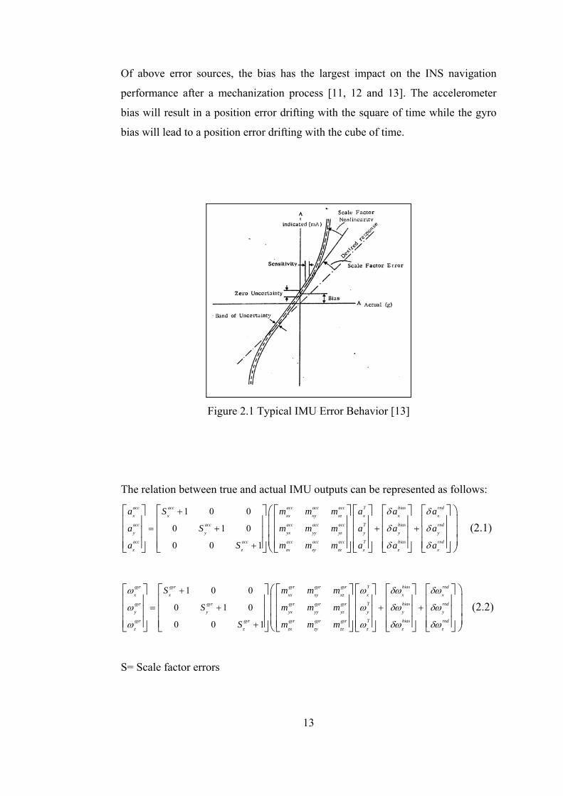
Of above error sources, the bias has the largest impact on the INS navigation
performance after a mechanization process [11, 12 and 13]. The accelerometer
bias will result in a position error drifting with the square of time while the gyro
bias will lead to a position error drifting with the cube of time.
Figure 2.1 Typical IMU Error Behavior [13]
The relation between true and actual IMU outputs can be represented as follows:
1 0 0
0 1 0
0 0 1
+
= + + +
+
⎡ ⎤ ⎡ ⎤ ⎡ ⎤ ⎡ ⎤ ⎡ ⎤ ⎡⎢ ⎥ ⎢ ⎥ ⎢ ⎥ ⎢ ⎥ ⎢ ⎥ ⎢⎢ ⎥ ⎢ ⎥ ⎢ ⎥ ⎢ ⎥ ⎢ ⎥⎢ ⎥ ⎢ ⎥ ⎢ ⎥ ⎢ ⎥ ⎢ ⎥⎣ ⎦ ⎣ ⎦ ⎣ ⎦ ⎣ ⎦ ⎣ ⎦ ⎣
acc acc acc acc acc T bias rnd
x x xx xy xz x x x
acc acc acc acc acc T bias rnd
y y yx yy yz y y y
acc acc acc acc acc T bias rnd
z z zx zy zz z z z
a S m m m a a a
a S m m m a a a
a S m m m a a a
δ δ
δ δ
δ δ
⎛ ⎤ ⎞⎜ ⎟⎥⎜ ⎟⎢ ⎥⎜ ⎟⎢ ⎥⎝ ⎦ ⎠
(2.1)
1 0 0
0 1 0
0 0 1
+
= + + +
+
⎡ ⎤ ⎡ ⎤ ⎡ ⎤ ⎡ ⎤ ⎡ ⎤ ⎡⎢ ⎥ ⎢ ⎥ ⎢ ⎥ ⎢ ⎥ ⎢ ⎥ ⎢⎢ ⎥ ⎢ ⎥ ⎢ ⎥ ⎢ ⎥ ⎢ ⎥⎢ ⎥ ⎢ ⎥ ⎢ ⎥ ⎢ ⎥ ⎢ ⎥⎣ ⎦ ⎣ ⎦ ⎣ ⎦ ⎣ ⎦ ⎣ ⎦ ⎣
gyr gyr gyr gyr gyr T bias rnd
x x xx xy xz x x x
gyr gyr gyr gyr gyr T bias rnd
y y yx yy yz y y y
gyr gyr gyr gyr gyr T bias rnd
z z zx zy zz z z z
S m m m
S m m m
S m m m
ω ω δω δω
ω ω δω δω
ω ω δω δω
⎛ ⎤ ⎞⎜ ⎟⎥⎜ ⎟⎢ ⎥⎜ ⎟⎢ ⎥⎝ ⎦ ⎠
(2.2)
S= Scale factor errors
14
m= Misalignment errors
Bias =Constant errors
Rnd= Random noise errors
In the above equations, acca and gyrω represent the actual IMU outputs whereas,
Ta and Tω denotes true values. Take notice that this error model is in a simplified
form which otherwise can be written in nonlinear form and can include some
other terms, such as scale factor nonlinearities, g2 dependent terms etc.
2.2 Inertial Navigation System
An inertial navigation system is a unit which gets inertial data (angular rate and
acceleration) from an IMU, calculates position, velocity and attitude information
with respect to a known grid system or reference frame by utilizing 6 degree of
freedom kinematics equations. Basically, an INS continuously integrates
acceleration and angular rates to obtain velocity, position, and angular position.
Generally, inertial navigation systems have high bandwidth, high data output rate
and high accuracy in short duration.
An attitude-heading reference is a dead-reckoning system which provides
continuous attitude, heading, position, and velocity information. It is neither a
slaved directional gyrocompass system nor a vertical gyroscope, but a
compromise to both that provides low-accuracy position and velocity (but with
unbounded errors) information. Advanced AHRS systems in use today employ
strapdown ring laser gyros (RLG) and/or fiber-optic gyros; that is, the sensors are
“bolted” to the aircraft structure and not isolated using gimbals.
15
Due to its nature, an INS/AHRS suffers from stability. Accelerometers and gyros
have different kind of errors (bias, noise etc.). When an INS integrates inertial
data, all errors in the inertial sensors accumulate, resulting in a performance
decrease in long term. Also, any error in gravity and world shape models result in
errors similar to sensor errors. However, an INS is perfect for short term
navigation requirements. A navigation system designer should choose IMU
performance specifications according to the following criteria;
• Accuracy requirements • Dynamics of the host system
The primary object is to determine the position and attitude accuracy
requirements. Choosing a suitable set of inertial sensors is accomplished by
optimizing between price and performance. Through the integration process, all
inertial sensor errors accumulate, thus as the total integration time increases,
navigation errors accumulate. The dynamics of the platform (e.g. manoeuvres
done by the host platform) excites some of the inertial sensor errors (scale factor
errors, g dependent errors etc.).
Nowadays, many integrated systems use GPS, TERCOM, DSMAC, star sensors
etc. to have a stable position and velocity solution. [3, 11].
2.2.1 Inertial Navigation Mechanization Equations
In this part of the thesis, basic components of inertial navigation kinematics will
be introduced.
2.2.1.1 Reference Coordinate Frames
Many reference frames are defined in inertial navigation systems. The IMU
outputs (acceleration and rotational rates) are expressed in body coordinates, but

16
the velocity is generally expressed in navigation frames. In this section, the
fundamental reference frames that are used in navigation systems are defined [19]
2.2.1.1.1 Inertial Frame
The inertial frame (denoted as i frame), is an ideal coordinate frame, where the
coordinate frame itself has no acceleration or rotational rates, in other words an
ideal IMU gives zero output if it attached to an inertial frame. Unfortunately, an
inertial frame is difficult to express in real world, so a quasi inertial frame is
generally used. This quasi inertial frame has its origin at the centre of the Earth
and axes that are non-rotating with respect to distant stars. Z axis is along the spin
axis of the Earth, x axis points towards the mean vernal equinox, and y axis
completes the famous right hand rule.
2.2.1.1.2 Earth frame
The Earth (e) frame has its origin at the centre of the Earth and axes fixed with
respect to the Earth. X axis points toward the mean meridian of Greenwich in
equatorial plane, Z axis is parallel to mean spin axis of the Earth and again Y axis
completes the right hand rule.
Earth frame continuously rotates with respect to inertial frame with an angular
velocity of;
[0 0 ]eieω = Ω (2.3)
Here, Ω is the angular speed of the earth. Its value is;
Ω =7.2921158 rad/day
17
In the Earth frame, the position of the host platform is expressed in terms of its
latitude, longitude, and altitude.
2.2.1.1.3 Navigation frame
The navigation frame is a local geodetic frame which has its origin coinciding
with that of the IMU, with x axis pointing toward geodetic North, its z axis
orthogonal to the reference ellipsoid pointing downward, and again y axis
complies the right hand rule. The Navigation frame is also known as North East
down (NED) frame.
2.2.1.1.4 Computer frame
The computer frame is the frame that is used by the navigation computer. With an
ideal inertial navigation system (no IMU errors, no computational errors etc.), the
computer frame is exactly the same as the navigation frame. In the real world,
there is a difference between the navigation and computer frames.
The transformation matrix between computer and navigation frames is expressed
in navigation error equations.
2.2.1.2 Coordinate Transformation
A coordinate transformation is used to express the components of a vector in a
different coordinate frame. Coordinate transformation matrices are orthogonal
matrices and their determinants are equal to one provided that right-handed
Cartesian coordinate systems are used. There are different methods to transform a
vector between different coordinate frames, such as direction cosine matrix,
18
quaternion etc. In this thesis, direction cosine matrices that are obtained by
successive Euler rotations are used.
2.2.1.3 Earth Shape Model
In order to determine position on the Earth using inertial measurements, it is
necessary to make some assumptions regarding the shape of the Earth. Owing to
the slight flattening of the Earth at the poles, Earth is modeled as a reference
ellipsoid which approximates more closely to the true geometry. Generally,
WGS84 model [1, 2, 3 and 8] is used as the earth shape model. In this model,
following parameters are introduced;
R: The length of the semi major axis (~6378 km)
(1 )r R f= − : The length of the semi minor axis (~6356 km)
( ) /f R r R= − : The flattening of the ellipsoid (~1/298.25)
(2 )e f f= − : The major eccentricity of the ellipsoid (~0.08188)
With these parameters defined, the meridian radius of curvature ( NR ) and the
transverse radius of curvature ( ER ) may be derived as;
2
32 2 2
(1 )
(1 sin )N
R eRe L
−=
− (2.4)
12 2 2(1 sin )
ERR
e L=
− (2.5)
Here, L is latitude.
19
2.2.1.4 Gravitational Acceleration Model
As mentioned earlier, an accelerometer can only measure the difference between
the gravitational acceleration and the acceleration of the body with respect to the
inertial frame. In order to obtain the velocity and position data, an accurate model
of the gravitational field is needed. In the related literature, there are different
gravity models that are used in navigation applications. Ideally, the gravity vector
is assumed to be acting vertically downwards to the reference ellipsoid, which is
not the case in the real world due to anomalies. In this thesis, the model given in
[11] is used. In this model, gravity at the surface of the reference ellipsoid (zero
altitude) is given as;
3 2 6(0) 9.7803267714(1 5.3024.10 .sin 5.9.10 .sin 2 )g L L− −= + − (2.6)
And the change of magnitude of gravity with respect to altitude is given as;
2
(0)( )(1 / )
gg hh R
=+
(2.7)
Here, h is gathered from INS outputs.
2.2.1.5 Inertial Frame mechanization
Dominant INS errors are caused by imperfect knowledge of initial conditions (for
example, those existing after alignment) and by error propagation in time. The
nine, nonlinear differential navigation equations (3 velocity, 3 position, 3 attitude
equation) can be perturbed by a wide variety of error sources, not only those
resulting from incorrect initial conditions. The perturbations of these equations,
when kept small, can be shown to result in a linear set of differential equations.
The most popular set of these equations is called the Pinson error model, named
after the man who derived it [14, 15, 16].
20
Remember that errors are both deterministic and statistical, and the statistical
errors can only be estimated. Investigating the propagation of deterministic errors
may provide a useful insight into system performance, but there is such a wide
variety of error sources that one is never totally sure which ones are dominating
the error response curves.
In this system, it is required to calculate the vehicle speed with respect to earth,
the ground speed, in inertial axes, denoted by iev . The differential equations for
velocity, position and attitude can expressed as follows;
. (2. )= − + × +n n b ne b ie en e pv C a v gω ω (2.8)
=+N
N
VLR h
(2.9)
sec( )=
+E
N
V LlR h
(2.10)
= − Dh V (2.11)
( )=n n bb b nbC C ω (2.12)
where;
nev : velocity of the host platform
L: latitude
l: longitude
21
nbC : direction cosine matrix relating body and navigation frame.
h: altitude
na : acceleration to which the inertial measurement unit is subjected
enω :Transport rate, whic can be expressed as;
[ /( ) /( ) . tan( ) /( )]nen E e N n E eV R h V R h V L R hω = + − + − + (2.13)
ieω : Earth rotation rate
pg : Gravity vector
bnbω :The angular rate of the body with respect to the navigation frame
bnbω can be expressed as the measured body rates ( b
ibω ) and estimates of the
components of the navigation frame rate ( in ie enω ω ω= + ) ;
.( )b b n n nnb ib b ie enCω ω ω ω= − + (2.14)
Detailed derivation of the navigation mechanization equations are given in
Appendix C.
22
2.2.2 Error Model of Inertial Navigation Systems
The navigation computer of an INS is essentially a differential equation solver.
The navigation mechanization equations represent a nonlinear, time varying
system. This system is unstable in the sense of Liapunov. Therefore, every
disturbance that affects the system causes the output errors to grow unbounded.
The rate at which errors grow are determined by the source of error and the
trajectory that system follows. For the INS systems, major error sources can be
classified into 3 groups [10, 15]:
1. IMU Errors (Input Errors)
2. Initialization Errors (Initial state Errors)
3. Computation Errors
The discrete and quantized nature of navigation processors tends to produce some
computational errors on navigation solution. This situation arises especially in
high vibratory environments. The importance of this kind of error depends on the
fact that this error can neither be estimated nor compensated. Therefore this error
sets a lower limit in the accuracy of inertial navigation system. For the real
implementation (when real IMU increments are used), with the use of appropriate
conning and sculling algorithms and sufficient processing frequency,
computational errors can be reduced to very low levels. However, one should be
very careful when designing a simulation environment in computer. In a computer
simulation implementation, calculating simulated velocity and angle increments
instead of acceleration and rotation rate can be very difficult under vibratory
environments (i.e. vibrations in the host platform). Usually, this difficulty is
handled by simply taking Euler integration of the calculated acceleration and
rotation rate to obtain associated increments. However, such an operation causes
computational errors to grow significantly. Therefore, when developing a
23
simulation environment in computer, this point should always be considered, and
necessary precautions should be taken to reduce the effect of computational errors
during simulations.
As the navigation mechanization equations are nonlinear, they cannot be applied
to a linear estimation filter, namely Kalman filter. That’s why the error model of
navigation states. The error propagation equations are derived by first order
perturbations assuming small attitude errors. The error model of attitude, velocity
and position is expressed as follows;
.= − − × +n n b n n nb ib in inCγ δω ω γ δω (2.15)
( . ) . (2. )
(2. )
= × + − × × +
− + × +
n n b n n b n n n ne b b e ie en
n n nie en e p
v C a C a v
v g
δ γ δ ω ε δω
ω ω δ δ (2.16)
= Dh Vδ δ (2.17)
/( ) . /( )= + − +N n N nL V R h V h R hδ δ δ (2.18)
.sec( ) /( ) .sec( ). tan( ). /( ).sec( ). /( )
= + + +− +
E e E e
E e
l V L R h V L L L R hV L h R h
δ δ δ δδ δ
(2.19)
nγ : Error misalignment vector that relates navigation and computer frame
Lδ : Error in latitude
lδ : Error in longitude
24
Vδ : Velocity error vector
hδ : Altitude error
bibδω : Errors in gyro measurements
ninδω : Errors in n
inω , which is expressed as;
n n nin ie enδω δω δω= + (2.20)
2
2 2
( ). tan( ) . tan( ) .
( ) ( )(cos( ))
⎡ ⎤−⎢ ⎥+ +⎢ ⎥
⎢ ⎥= −⎢ ⎥+ +⎢ ⎥
⎢ ⎥− −+ −⎢ ⎥
+ + +⎣ ⎦
E E
E E
n N Nen
N N
N N N
E E E
V V hR h R hV V h
R h R hV L V L h VR h R h R h L
δ δ
δ δδω
δ δ
(2.21)
[ sin( ) 0 cos( ) ]n Tie L L L Lδω δ δ= −Ω −Ω (2.22)
The detailed derivation of the linear error equations are given in Appendix D.
25
CHAPTER 3
3 MAGNETOMETERS
3.1 World Magnetic Model
World magnetic model (WMM)[7] is a tool to obtain the Earth’s ideal magnetic
field model at any point on the Earth. WMM gives the model in terms of spherical
harmonic series. The coefficients of the model is updated every five years. The
outputs of the model are magnetic field values in NED components. The details of
WMM 2005 is given in Appendix A
3.1.1 Alternative Magnetic Field Model
World magnetic field model is global model that is the model theoretically works
in any point of the world, but having some problems An alternative model is
proposed with the following assumptions;
• Magnetic field is approximately constant in a local field, i.e., the
horizontal position change is limited to 10km, and vertical position change
is limited to 1km.
• The sensor errors are negligible.
The mathematical relation between the reference magnetic field and the
magnetometer measurements is as bellows;
26
.( )=N N BBB C B (3.1)
Where NB = Reference Magnetic field given by WMM2005 BB = Magnetic field measurement by magnetometer NBC = Direction Cosine matrix relating navigation and body frames.
If attitude information of the host platform ( NBC ) and magnetometer
measurements ( )BB are known, it is possible to find the reference magnetic field
vector in every navigated point. In this alternative model, two error sources
occur;
• INS errors (gyro errors especially)
• Magnetometer errors
INS errors can be minimized by using multiple aiding sources (DGPS, DSMAC,
TERCOM etc.). As it will be explained in this chapter, magnetometer errors are
negligible.
This method has two deficiencies arising from its assumptions. The developed
method only works in a local navigation case (short range missiles, UAVs, mobile
robots). On the other hand, neither the magnetometer nor the gyros are perfect
sensors; the sensor errors will affect the magnetic field solution. High accurate
gyros (e.g., Ring laser or fiber optic gyros) and magnetometers must be used.
Although this method has some advantages to the WMM, it must be
experimentally proven before it can be used. Difficulties in this process are as
follows;
• High Accuracy Magnetometer Requirement: In order to have an accurate
model, the magnetometer should have high accuracy,
27
• DGPS aided navigation unit: As it can be seen from equation 3.1, the
accuracy of the resultant magnetic field model depends on the accuracy of
the attitude information. High accuracy, navigation grade (e.g.., RLG,
FOG) gyros must be used to have an accurate model.
Any error in attitude and magnetic field measurements will result in error in the
resultant model, so the magnetometers and gyros should have very high accuracy.
As these units are very expensive, the accuracy of this magnetic model could not
be proven in this study. Thus, WMM 2005 will be used in this thesis.
3.2 Magnetometer Types
Magnetic sensors differ from most other detectors in that they do not directly
measure the physical property of interest [24]. Devices that monitor properties
such as temperature, pressure, strain, or flow provide an output that directly
reports the desired parameter. Magnetic sensors, on the other hand, detect
changes, or disturbances, in magnetic fields that have been created or modified,
and from them derive information on properties such as direction, presence,
rotation, angle, or electrical currents. The output signal of these sensors requires
some signal processing for translation into the desired parameter. Although
magnetic detectors are somewhat more difficult to use, they do provide accurate
and reliable data — without physical contact [24].
Magnetic sensors can be classified according to low-, medium-, and high-field
sensing range. In this study, devices that detect magnetic fields <1 µG (micro
Gauss) are considered low-field sensors; those with a range of 1 µG to 10 G are
Earth's field sensors; and detectors that sense fields >10 G are referred to as bias
magnet field sensors.
A magnetic field is a vector quantity with both magnitude and direction. The
scalar sensor measures the field's total magnitude but not its direction. The omni
directional sensor measures the magnitude of the component of magnetization that
lies along its sensitive axis. The bidirectional sensor includes direction in its
28
measurements. The vector magnetic sensor incorporates two or three bidirectional
detectors. Some magnetic sensors have a built-in threshold and produce an output
only when it is surpassed.
3.3 Magnetometer Error Sources
Magnetometer accuracy is affected by [25]:
1. Magnetic sensor errors
2. Temperature effects
3. Nearby ferrous materials
4. Variation of the earth's field
Solid state magneto-resistive (MR) sensors available today can reliably resolve
<0.07 mgauss fields. This is more than a five times margin over the 0.39 mgauss
field required to achieve 0.01° resolution. Other magnetic sensor specifications
should support field measurement certainty better than 0.005° to maintain an
overall 0.01° heading accuracy. These include the sensor noise, linearity,
hysteresis, and repeatability errors. Any gain and offset errors of the magnetic
sensor will be compensated for during the hard iron calibration (discussed later)
and will not be considered in the error budget. MR sensors can provide a total
error of less than 0.1 mgauss [24, 25].
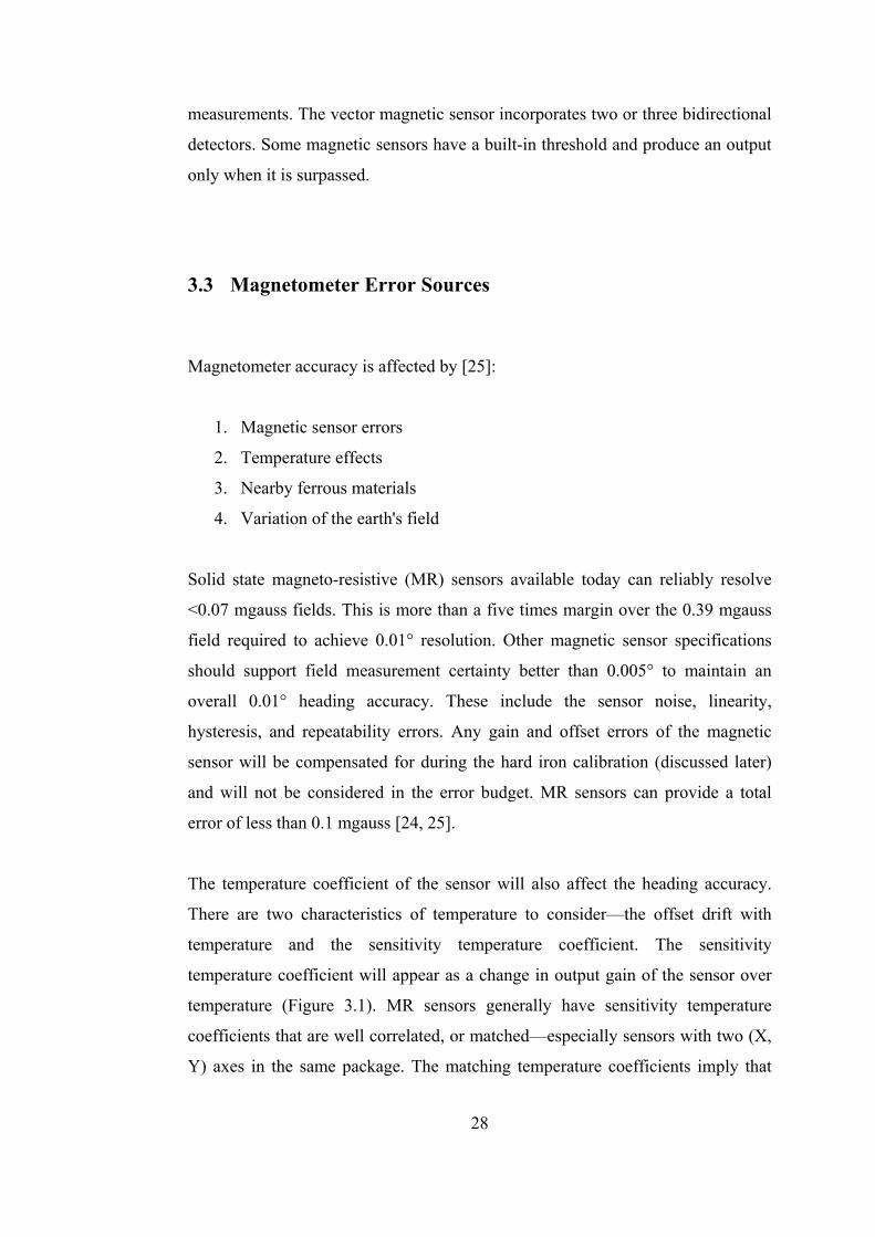
The temperature coefficient of the sensor will also affect the heading accuracy.
There are two characteristics of temperature to consider—the offset drift with
temperature and the sensitivity temperature coefficient. The sensitivity
temperature coefficient will appear as a change in output gain of the sensor over
temperature (Figure 3.1). MR sensors generally have sensitivity temperature
coefficients that are well correlated, or matched—especially sensors with two (X,
Y) axes in the same package. The matching temperature coefficients imply that
29
the output change over temperature of the X axis will track the change in output
of the Y axis. This effect will cancel itself since it is the ratio of Y over X that is
used in the heading calculation [Azimuth = arcTan(Y/X)]. For example, as the
temperature changes the Y reading by 12%, it also changes the X reading by 12%
and the net change is canceled. The only consideration is then the dynamic input
range of the A/D converter. The magnetic sensor offset drift with temperature is
not correlated and may in fact drift in opposite directions. This will have a direct
affect on the heading and can cause appreciable errors. There are many ways to
compensate for temperature offset drifts using digital and analog circuit
techniques. A simple method to compensate for temperature offset drifts in MR
sensors is to use a switching technique referred to as set/reset switching. This
technique cancels the sensor temperature offset drift, and the dc offset voltage as
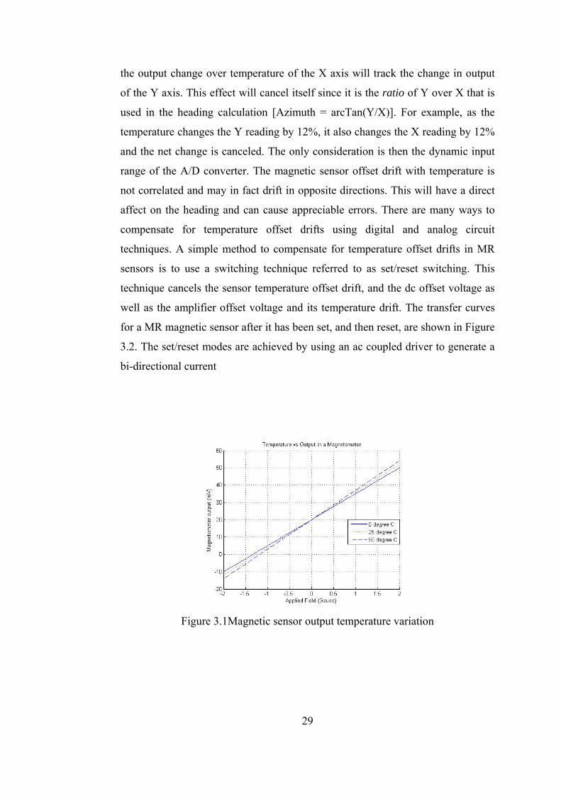
well as the amplifier offset voltage and its temperature drift. The transfer curves
for a MR magnetic sensor after it has been set, and then reset, are shown in Figure
3.2. The set/reset modes are achieved by using an ac coupled driver to generate a
bi-directional current
Figure 3.1Magnetic sensor output temperature variation
30
Figure 3.2 Set and reset output transfer curves.
The two curves result from an inversion of the gain slope with a common
crossover point at the offset voltage. For the sensor in Figure 3.2, the sensor offset
is –3 mV. This offset is not desirable and can be eliminated using the set/reset
switching technique described below. Other methods of offset compensation are
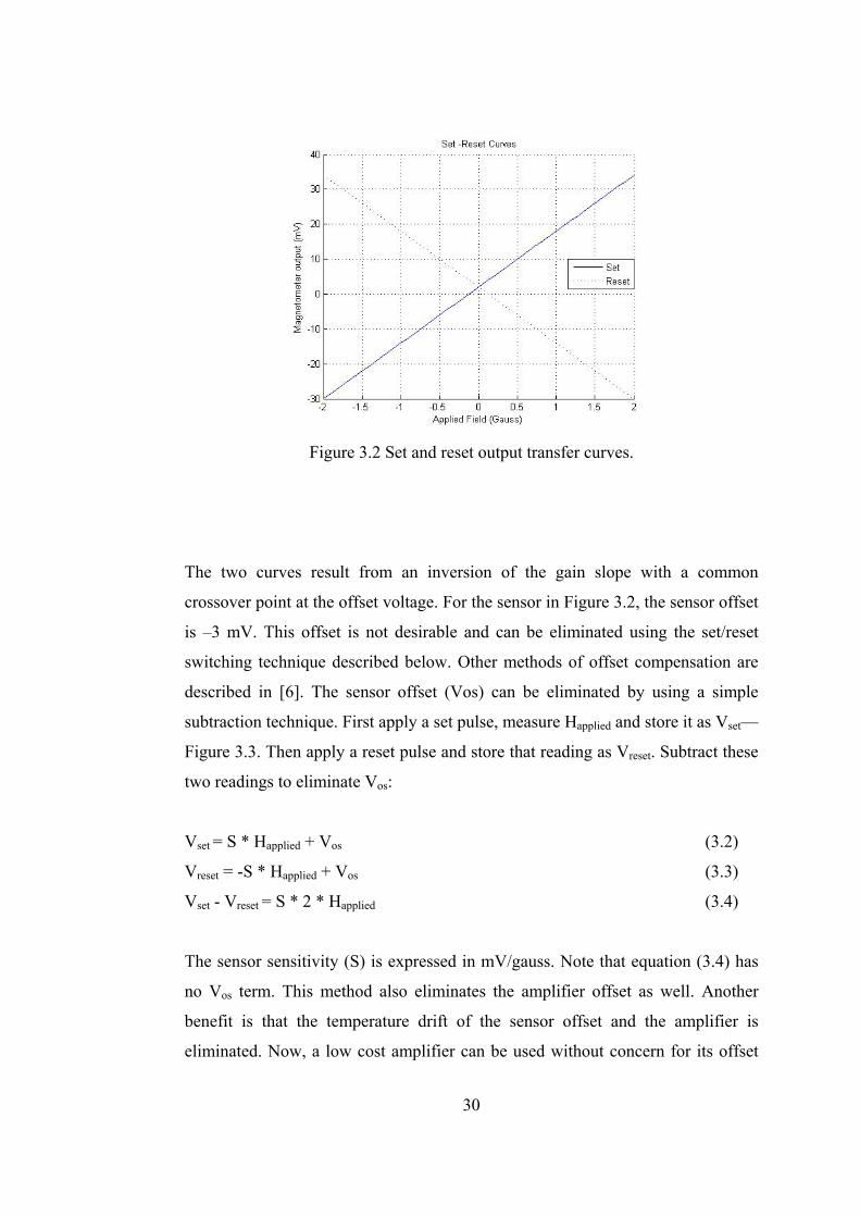
described in [6]. The sensor offset (Vos) can be eliminated by using a simple
subtraction technique. First apply a set pulse, measure Happlied and store it as Vset—
Figure 3.3. Then apply a reset pulse and store that reading as Vreset. Subtract these
two readings to eliminate Vos:
Vset = S * Happlied + Vos (3.2)
Vreset = -S * Happlied + Vos (3.3)
Vset - Vreset = S * 2 * Happlied (3.4)
The sensor sensitivity (S) is expressed in mV/gauss. Note that equation (3.4) has
no Vos term. This method also eliminates the amplifier offset as well. Another
benefit is that the temperature drift of the sensor offset and the amplifier is
eliminated. Now, a low cost amplifier can be used without concern for its offset
31
effects. This is a powerful technique and is easy to implement if the readings are
controlled by a low cost microprocessor. Using this technique to reduce
temperature effects can drop the overall variation in magnetic readings to less than
0.01%/°C. This amounts to less than 0.29° effect on the heading accuracy over a
50°C temperature change [25].
Figure 3.3 Set and reset effect on sensor output (Vout) [25]
Another consideration for heading accuracy is the effects of nearby ferrous
materials on the earth's magnetic field. Since heading is based on the direction of
the earth's horizontal field (Xh,Yh), the magnetic sensor must be able to measure
this field without influence from other nearby magnetic sources or disturbances.
The amount of disturbance depends on the material content of the platform and
connectors as well as ferrous objects moving near the magnetometer. When a
ferrous object is placed in a uniform magnetic field it will create disturbances as
shown in Figure 3.4. This object could be a steel bolt or bracket near the
magnetometer or an iron door latch close to the magnetometer. The net result is a
characteristic distortion, or anomaly, to the earth’s magnetic field that is unique to
32
the shape of the object. Before looking at the effects of nearby magnetic
disturbances, it is beneficial to observe an ideal output curve with no disturbances.
When a two-axis (X,Y) magnetic sensor is rotated in the horizontal plane, the
output plot of Xh vs. Yh will form a circle centered at the (0,0) origin (see Figure
3.5). If a heading is calculated at each point on the circle, the result will be a linear
sweep from 0° to 360°.
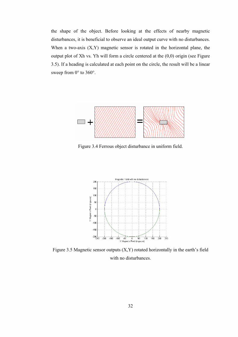
Figure 3.4 Ferrous object disturbance in uniform field.
Figure 3.5 Magnetic sensor outputs (X,Y) rotated horizontally in the earth’s field
with no disturbances.
33
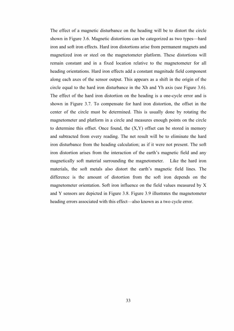
The effect of a magnetic disturbance on the heading will be to distort the circle
shown in Figure 3.6. Magnetic distortions can be categorized as two types—hard
iron and soft iron effects. Hard iron distortions arise from permanent magnets and
magnetized iron or steel on the magnetometer platform. These distortions will
remain constant and in a fixed location relative to the magnetometer for all
heading orientations. Hard iron effects add a constant magnitude field component
along each axes of the sensor output. This appears as a shift in the origin of the
circle equal to the hard iron disturbance in the Xh and Yh axis (see Figure 3.6).
The effect of the hard iron distortion on the heading is a one-cycle error and is
shown in Figure 3.7. To compensate for hard iron distortion, the offset in the
center of the circle must be determined. This is usually done by rotating the
magnetometer and platform in a circle and measures enough points on the circle
to determine this offset. Once found, the (X,Y) offset can be stored in memory
and subtracted from every reading. The net result will be to eliminate the hard
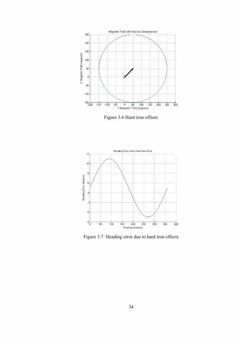
iron disturbance from the heading calculation; as if it were not present. The soft
iron distortion arises from the interaction of the earth’s magnetic field and any
magnetically soft material surrounding the magnetometer. Like the hard iron
materials, the soft metals also distort the earth’s magnetic field lines. The
difference is the amount of distortion from the soft iron depends on the
magnetometer orientation. Soft iron influence on the field values measured by X
and Y sensors are depicted in Figure 3.8. Figure 3.9 illustrates the magnetometer
heading errors associated with this effect—also known as a two cycle error.
34
Figure 3.6 Hard iron offsets
Figure 3.7 Heading error due to hard iron effects
35
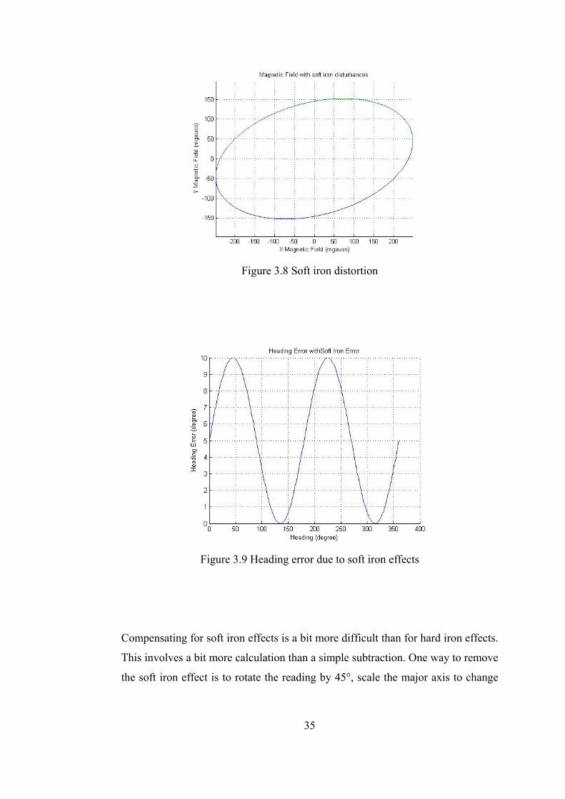
Figure 3.8 Soft iron distortion
Figure 3.9 Heading error due to soft iron effects
Compensating for soft iron effects is a bit more difficult than for hard iron effects.
This involves a bit more calculation than a simple subtraction. One way to remove
the soft iron effect is to rotate the reading by 45°, scale the major axis to change
36
the ellipse to a circle, and then rotate the reading back by 45°. This will result in
the desired circular output response shown in Figure 3.9. Most ferrous material in
vehicles tends to have hard iron characteristics. The best approach is to eliminate
any soft iron materials near the magnetometer and deal with the hard iron effects
directly. It is also recommended to degauss the platform near the magnetometer
prior to any hard/soft iron compensation. Some magnetometer manufacturers
provide calibration methods to compensate for the hard and soft iron effects. Each
calibration method is associated with a specified physical movement of the
magnetometer platform in order to sample the magnetic space surrounding the
magnetometer. The calibration procedure can be as simple as pointing the host in
three known directions, or as complicated as moving in a complete circle with
pitch and roll, or pointing the host in 24 orientations including variations in tilt. It
is impossible for a marine vessel to perform the 24- point calibration, but easy for
a hand-held platform. If the magnetometer is only able to sample the horizontal
field components during calibration, then there will be uncompensated heading
errors with tilt. Heading error curves can be generated for several known headings
to improve heading accuracy Hard and soft iron distortions will vary from
location to location within the same platform. The magnetometer has to be
mounted permanently to its platform to get a valid calibration. A particular
calibration is only valid for that location of the magnetometer. If the
magnetometer is reoriented in the same location, then a new calibration is
required. A gimbaled magnetometer can not satisfy these requirements and hence
the advantage of using a strapdown, or solid state, magnetic sensor. It is possible
to use a magnetometer without any calibration if the need is only for repeatability
and not accuracy.
The final consideration for heading accuracy is the variation, or declination, angle.
It is well known that the earth's magnetic poles and its axis of rotation are not at
the same geographical location. They are about 11.5° away from each other. This
creates a difference between the true north, or grid north, and the magnetic north,
or direction a magnetic magnetometer will point. Simply it is the angular
difference between the magnetic and true north expressed as an Easterly or
37
Westerly variation. This difference is defined as the variation angle and is
dependent on the magnetometer location—sometimes being as large as 25°. To
account for the variation simply add, if Westerly, or subtract, if Easterly, the
variation angle from the corrected heading computation. The variation angles have
been mapped over the entire globe. For a given location the variation angle can be
found by using a geomagnetic declination map or a GPS (Global Positioning
System) reading and an IGRF model. The International Geomagnetic Reference
Field (IGRF) or World Magnetic Model (WMM) is a series of mathematical
models describing the earth's field and its time variation After heading is
determined, the variation correction can be applied to find true north according to
the geographic region of operation.
The performance of a magnetometer will greatly depend on its installation
location. A magnetometer depends on the earth’s magnetic field to provide
heading. Any distortions of this magnetic field by other sources should be
compensated for in order to determine an accurate heading. Sources of magnetic
fields include permanent magnets, motors, electric currents—either dc or ac, and
magnetic metals such as steel or iron. The influence of these sources on
magnetometer accuracy can be greatly reduced by placing the magnetometer far
from them. Some of the field effects can be compensated by calibration. However,
it is not possible to compensate for time varying magnetic fields; for example,
disturbances generated by the motion of magnetic metals, or unpredictable
electrical current in a nearby wire. Magnetic shielding can be used for large field
disturbances from motors or speakers. The best way to reduce disturbances is
distance. Also, never enclose the magnetometer in a magnetically shielded
metallic housing.
The effects of nearby magnetic distortions can be calibrated out of the
magnetometer readings once it is secured to the platform. Caution must be taken
in finding a magnetometer location that is not too near varying magnetic
disturbances and soft iron materials. Shielding effects from speakers and high
current conductors near the magnetometer may be necessary. Variations in the

38
earth's field from a true north heading can be accounted for if the geographical
location of the magnetometer is known. This can be achieved by using a map
marked with the deviation angles to find the correct heading offset variation; or
use a GPS system and the IGRF reference model to compute the variation angle.
Low cost magnetometeres of the type described here are susceptible to temporary
heading errors during accelerations and banked turns. The heading accuracy will
be restored once these accelerations diminish. With a strapdown magnetometer
there is no accuracy drift to worry about since the heading is based on the true
earth's magnetic field. They tend to be very rugged to shock and vibrations
effects and consume very low power and are small in size
39
CHAPTER 4
4 KALMAN FILTER
Navigation outputs—position, velocity, and attitude (PVA) — must be updated in
order to be bounded. Kalman filter provides the manner and the method for
combining updates that is practically useful as well as mathematically ingenious.
Moreover, this technique can be extended to the integration of outputs from a
wide variety of systems and continues to show a high degree of practical utility in
navigation applications.
The Kalman filter is a linear filter. Recall that the actual differential equations for
INS operation are non-linear, but the error equations are valid for linearized
versions of these differential equations. Hence the requirement for the errors
themselves to remain small, otherwise a linear analysis is not valid. Kalman filter
applications presume that state-space dynamic modeling will be used to
implement the algorithm. In the next part of this chapter the discrete Kalman
filter in its most universal form will be presented and derived in a straightforward
manner. Only those parts of the derivation will be emphasized that have practical
significance for flight applications [26, 27, 28, 29].
40
4.1 Kalman Filter
4.1.1 Motivation for the Kalman Filter for INS
The major problems that exist if one relies on an inertial navigation system in
motion:
• How to correct the navigation error equations while flying so that they
remain useful even though the initial navigation errors were not known
accurately.
• How to deal with noisy measurements from a variety of other systems that
are arriving at different times; how to estimate the covariance of the INS
output whenever an update could occur to see how much of the
measurement should be believed in the presence of noisy system
dynamics;
• How to obtain estimates for all navigation outputs even though only one or
two is being measured by other means, providing as a result the most
probable position.
The Kalman filter can be used to solve all of these problems. The basic procedure
is;
• Initialize the filter by providing statistical estimates ox for the initial
navigation error states, their covariance P(t0), and noise covariance Q0 .
• Propagate both P(t0) and the ox to time of measurement update tk before
the measurement zk .
• Note that values before measurement are kP ( )− and kx ( )− .
• Compute the most probable estimate kx ( )+ by weighting kx ( )− and zk
with the Kalman gains.
If the filter converges, then it is possible to have a useable estimate of all the
navigation error states at all discrete times tk during the motion. Also estimate of
41
the covariance of the navigation error states are obtained and one can verify that it
decreases following a measurement update.
4.1.1.1 Kalman Filter Implementation
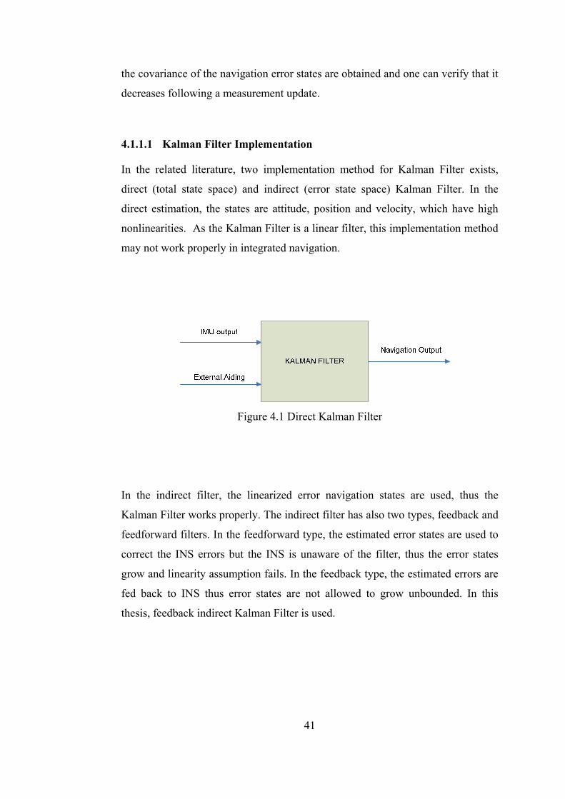
In the related literature, two implementation method for Kalman Filter exists,
direct (total state space) and indirect (error state space) Kalman Filter. In the
direct estimation, the states are attitude, position and velocity, which have high
nonlinearities. As the Kalman Filter is a linear filter, this implementation method
may not work properly in integrated navigation.
Figure 4.1 Direct Kalman Filter
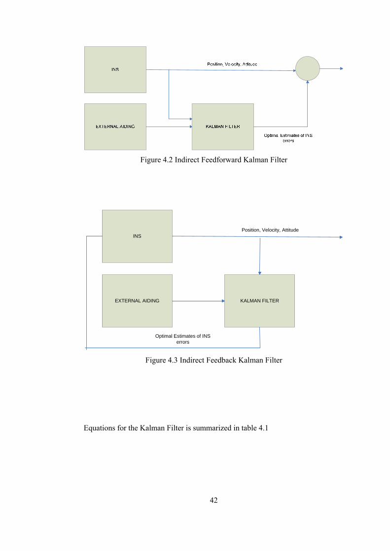
In the indirect filter, the linearized error navigation states are used, thus the
Kalman Filter works properly. The indirect filter has also two types, feedback and
feedforward filters. In the feedforward type, the estimated error states are used to
correct the INS errors but the INS is unaware of the filter, thus the error states
grow and linearity assumption fails. In the feedback type, the estimated errors are
fed back to INS thus error states are not allowed to grow unbounded. In this
thesis, feedback indirect Kalman Filter is used.
42
Figure 4.2 Indirect Feedforward Kalman Filter
KALMAN FILTER
INS
EXTERNAL AIDING
Position, Velocity, Attitude
Optimal Estimates of INS errors
Figure 4.3 Indirect Feedback Kalman Filter
Equations for the Kalman Filter is summarized in table 4.1
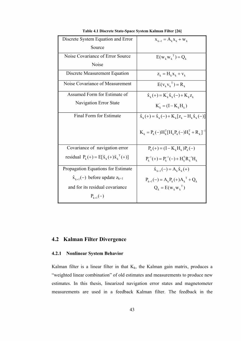
43
Table 4.1 Discrete State-Space System Kalman Filter [26]
Discrete System Equation and Error
Source k 1 k k kx A x w+ = +
Noise Covariance of Error Source
Noise
Tk k kE(w w ) Q=
Discrete Measurement Equation k k k kz H x v= +
Noise Covariance of Measurement Tk k kE(v v ) R=
Assumed Form for Estimate of
Navigation Error State
'k k k k kˆ ˆx ( ) K x ( ) K z + = − +
'k k kK (I K H )= −
Final Form for Estimate
k k k k k kˆ ˆ ˆx ( ) x ( ) K [z H x ( )]+ = − + − −
T T 1
k k k k k k kK P ( )H [H P ( )H R ]−= − − +
Covariance of navigation error
residual Tk k kP ( ) E[x ( )x ( )]+ = + +
k k k kP ( ) (I K H )P ( )+ = − −
1 1 T 1k k k k kP ( ) P ( ) H R H− − −+ = − +
Propagation Equations for Estimate
k 1x ( )+ − before update zk+1
and for its residual covariance
k 1P ( )+ −
k 1 k kˆ ˆx ( ) A x ( )+ − = +
Tk 1 k k k k
Tk k k
P ( ) A P ( )A Q
Q E(w w )+ − = + +
=
4.2 Kalman Filter Divergence
4.2.1 Nonlinear System Behavior
Kalman filter is a linear filter in that Kk, the Kalman gain matrix, produces a
“weighted linear combination” of old estimates and measurements to produce new
estimates. In this thesis, linearized navigation error states and magnetometer
measurements are used in a feedback Kalman filter. The feedback in the
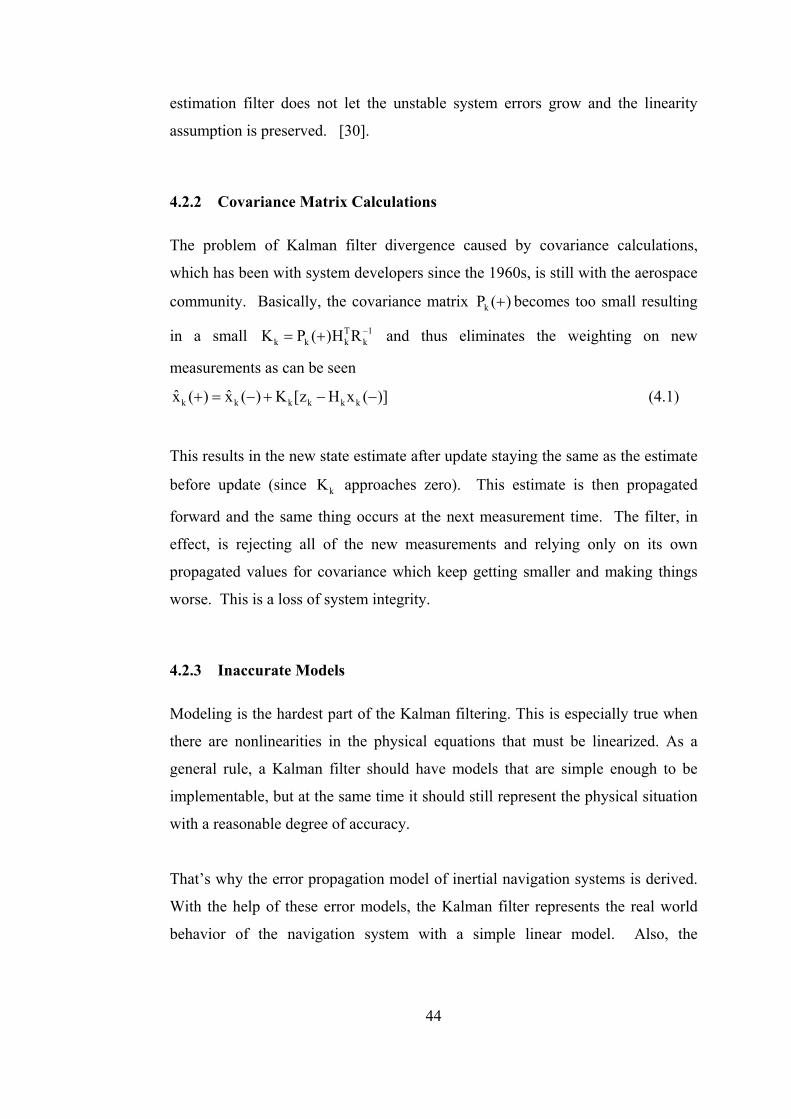
44
estimation filter does not let the unstable system errors grow and the linearity
assumption is preserved. [30].
4.2.2 Covariance Matrix Calculations
The problem of Kalman filter divergence caused by covariance calculations,
which has been with system developers since the 1960s, is still with the aerospace
community. Basically, the covariance matrix kP ( )+ becomes too small resulting
in a small T 1k k k kK P ( )H R−= + and thus eliminates the weighting on new
measurements as can be seen
k k k k k kˆ ˆx ( ) x ( ) K [z H x ( )]+ = − + − − (4.1)
This results in the new state estimate after update staying the same as the estimate
before update (since kK approaches zero). This estimate is then propagated
forward and the same thing occurs at the next measurement time. The filter, in
effect, is rejecting all of the new measurements and relying only on its own
propagated values for covariance which keep getting smaller and making things
worse. This is a loss of system integrity.
4.2.3 Inaccurate Models
Modeling is the hardest part of the Kalman filtering. This is especially true when
there are nonlinearities in the physical equations that must be linearized. As a
general rule, a Kalman filter should have models that are simple enough to be
implementable, but at the same time it should still represent the physical situation
with a reasonable degree of accuracy.
That’s why the error propagation model of inertial navigation systems is derived.
With the help of these error models, the Kalman filter represents the real world
behavior of the navigation system with a simple linear model. Also, the
45
measurement model of the magnetometer is derived in the same manner, it is
linear and accurate.
4.2.4 Measurement Acceptance/Rejection Criteria
If “outlier” measurements cannot be rejected, the navigation error will rapidly
grow without bound because the filter equations will ignore its own system
equations and become erratic. Measurement rejection criteria are normally based
on the “innovations” given by [ k k kˆz H x ( )− − ] or the equivalent [ kz kz ( )− − ]
which represents the “new information” that the measurement zk is providing
relative to what the filter estimates the measurement to be [ kz ( )− = k kˆH x ( )− ].
[28] recommends a 3-sigma test for this problem based on the innovations.
According to his scheme, if the magnitude of the ratio of the innovation to its
standard deviation is larger than 3, it is rejected, otherwise it is accepted. There
are no distinct criteria in this area, and once again the Monte Carlo data is
invaluable in testing the algorithms before it is in-motion tested. The sigma value
of a state is extracted from the related diagonal element of the covariance matrix,
kP ( )+ . The diagonal elements of kP ( )+ are the square of sigma (standard
deviation) of related states.
46
CHAPTER 5
5 ATTITUDE DETERMINATION WITH VECTOR
MEASUREMENTS
5.1 Attitude Determination with 2 Vector Sets
Let B represent the body frame and N represent the navigation frame. With a
single sensor that gives a vector output (e.g. magnetometer) VBsensor, it is not
possible to find the Euler angles that gives the transformation CBN between B and
N frames;
vBsensor = CB
N .vNreference (5.1)
By a single vector measurement, there exist infinitely many Euler angle solutions
[31]. To overcome this problem, a second vector measurement that is also
between B and N frame is used. Thus, 2 different vector sets (totally 4 vectors) are
ready for the attitude solution;
vB = CBN .vN uB = CB
N .uN (5.2)
By cross product of U and V vectors, W vector is obtained;
47
wB = uB × vB wN = uN × vN (5.3)
Using U, V and W, augmented matrix D is obtained;
DB3×3 = [uB
3×1 vB3×1 wB
3×1] DN3×3 = [uN
3×1 vN3×1 wN
3×1] (5.4)
Finally, CBN matrix can obtain as [33];
CBN = DB. (DN)-1 (5.5)
In order to obtain attitude from 5.5, UN3×1 and VN
3×1 should be non-collinear,
otherwise DN will be singular. For this kind of solution, two different vector
measurements are required. In coarse alignment procedure of navigation systems,
generally gravity and Earth rotation rates, which are certainly not parallel to each
other, are used for vector measurements [8, 32]. To measure the Earth rotation
rate (approx. 15deg/hr); the angular rate sensors must have a bias that is far less
than 15deg/hr, which is not the case in low cost gyros. To overcome this problem,
another kind of vector measurement should be taken. Three axis magnetometer
(TAM) is a good candidate for solution. Magnetic field and gravity are certainly
not parallel to each other. Thus, one has 4 vectors for attitude determination;
• Earth gravity field vector (defined in navigation frame)
• Accelerometer outputs( defined in body frame)
• Earth magnetic field vector (defined in navigation frame)
• Magnetometer field vector ( defined in body frame)
This kind of a solution requires the body to have accelerations except the
gravitational acceleration. In accelerating body, it is not possible to use gravity
field vector.
48
5.2 Magnetometer Measurement Models for Kalman Filter
Here we assume that the magnetometer has been calibrated for scale factors, non-
orthogonality corrections, and biases using one of the attitude independent
calibration algorithms. The body frame observation model of a TAM is similar to
a typical vector sensor [6,34,35]
.( )= +N N BB MgnB C B ν (5.6)
where BB is the TAM observation, NB is the reference magnetic field in an
Earth-fixed inertial frame corresponding to the specific position and altitude, NBC
is the ideal direction cosine matrix which is function of Euler angles , ,φ θ ψ , and
finally vk is the measurement noise that includes both sensor errors and
geomagnetic field model uncertainties,. The measurement noise is assumed to be
a zero-mean Gaussian process with covariance.
In terms of the DCM of computed navigation frame;
( . )( )= +N N N BB B MgnB C C Bδ ν (5.7)
Replacing NBCδ with the error misalignment vector,
( ). ( )= − +N n N BB MgnB I C Bγ ν (5.8)
Rearranging the equation
( ) . ( )= + − +N N B n N BB Mgn B MgnB C B C Bν γ ν (5.9)
. . . .− = −N N B N n N BB B Mgn BB C B C C Bν γ (5.10)
49
. ( . ) .− = × +N N B N B n NB B B MgnB C B C B Cγ ν (5.11)
Similarly, gravitational acceleration measurement can be written as;
.( )N N B bBg C a aδ= + (5.12)
Where baδ : Acceleration errors, such as bias scale factor, noise etc.
Following the same procedure in magnetometer measurements;
( )( )N N N B bB Bg C C a aδ δ= + + (5.13)
( ). ( )N C B bBg I C a aγ δ= − + (5.14)
( ) . ( )N C B b C B bB Bg C a a C a aδ γ δ= + − + (5.15)
. . . .N C B C b C BB B Bg C a C a C aδ γ− = − (5.16)
. ( . ) .− = × +N C B C B C bB B Bg C a C a C aγ δ (5.17)
In measurement equation (5.1), the states are three Euler angles given in nonlinear
form. To obtain a measurement equation which have error states (e.g. states that
model attitude errors), the relation between true and erroneous direction cosine
matrices are expressed;
A measurement equation directly for angular rates can be written by taking
derivative of equation (5.6);
50
. .
( . . )
( . ) . .
− −
= + × +
× + +
N N B N BB B
N B N B nB B
N B n N NB B Mgn B Mgn
B C B C B
C B C B
C B C C
γ
γ ν ν
(5.18)
Replacing nbC and nγ by
.( ) ( ).= −n n b n nb b ib in bC C Cω ω (5.19)
.= − − × +n n b n n nb ib in inCγ δω ω γ δω (5.20)
( .( ) ( ). ). .
(( .( ) ( ). ). . )
( . ) ( . )
( .( ) ( ). ). .
− − − =
− +
+ − − +
+ − +
N n b n n B N Bb ib in b B
n b n n B N B nb ib in b B
N B n b n n nB b ib in inn b n n Nb ib in b Mgn B Mgn
B C C B C B
C C B C B x
C B x C x
C C C
ω ω
ω ω γ
δω ω γ δω
ω ω ν ν
(5.21)
Same procedure can be applied to gravitational measurement equation.
With this equation, it is possible to estimate the angular rates. But, as this equation
is based on differentiation, all noisy measurements, magnetometer and gyro
outputs, are differentiated, which yields an extremely noisy measurement
equation. Magnetometers are generally low noise sensors, but the MEMS gyros
(especially MEMS gyros) can be very noisy. This measurement equation may
result in bad estimation if it is used in Kalman filter. In order to use these
equations, gyros should have low noise characteristics. In this thesis, low accuracy
MEMS gyros are taken into consideration, thus equation 5.21 cannot be used in
the simulation studies. This equation may be used in a case where low noise gyros
(such as RLG or FOG) are used.
5.3 Single Axis Attitude Determination
In spinning missiles, the roll rate can be as high as 7000-8.000 deg/s. Many gyros
will saturate in that kind of angular motion. Gyros that have such a measurement
range probably will have extremely high prices. As the guidance and autopilot
loops need the roll rate, it is crucial to estimate this roll motion.
51
Before analyzing the equations 5.30-5.36 and 5.41, it is important to note that in a
vector measurement equation set, three equations are not independent. Thus, it is
not possible to find all three Euler angles or rates analytically by a single vector
measurement, which is known as Wahba’s problem [31]. With a single vector,
only one Euler angle without ambiguity can be obtained provided that the other
two Euler angle should be known a priori.
Note that all three Euler angles are coupled to each other, thus if someone does
not know one of the angular speeds, it is not possible to calculate the Euler angles
due to the couplings. In the proposed algorithm, the following assumptions are
taken into consideration.
• The system has only one degree of rotational freedom, thus 2 Euler angles
are known a priori.
• If the system has three degree of freedom, then;
o The algorithm should run in such a high rate that the errors due to
Euler angle coupling between time steps are minimized.
o Three are three gyros, but one of them is saturated (e.g. it measures
1000 deg/s angular speed as 500 deg/s due to its measurement
range), thus the coupling errors again minimized.
The flow chart of this algorithm is given in Figure 5.1 .
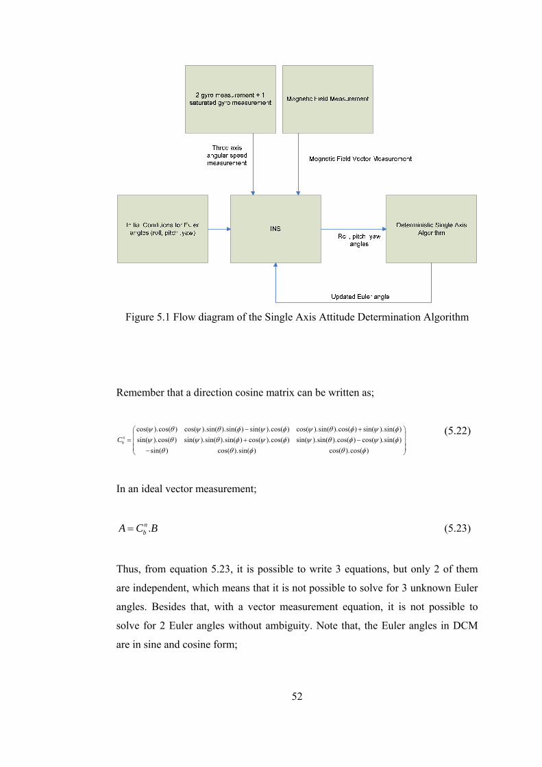
52
Figure 5.1 Flow diagram of the Single Axis Attitude Determination Algorithm
Remember that a direction cosine matrix can be written as;
cos( ).cos( ) cos( ).sin( ).sin( ) sin( ).cos( ) cos( ).sin( ).cos( ) sin( ).sin( )sin( ).cos( ) sin( ).sin( ).sin( ) cos( ).cos( ) sin( ).sin( ).cos( ) cos( ).sin( )
sin( ) cos( ).sin( ) cos( ).cos( )
− +⎛= + −
−
nbC
ψ θ ψ θ φ ψ φ ψ θ φ ψ φψ θ ψ θ φ ψ φ ψ θ φ ψ φ
θ θ φ θ φ
⎞⎜ ⎟⎜ ⎟⎜ ⎟⎝ ⎠
(5.22)
In an ideal vector measurement;
.= nbA C B (5.23)
Thus, from equation 5.23, it is possible to write 3 equations, but only 2 of them
are independent, which means that it is not possible to solve for 3 unknown Euler
angles. Besides that, with a vector measurement equation, it is not possible to
solve for 2 Euler angles without ambiguity. Note that, the Euler angles in DCM
are in sine and cosine form;
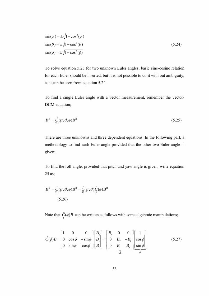
53
2
2
2
sin( ) 1 cos ( )
sin( ) 1 cos ( )
sin( ) 1 cos ( )
= ± −
= ± −
= ± −
ψ ψ
θ θ
φ φ
(5.24)
To solve equation 5.23 for two unknown Euler angles, basic sine-cosine relation
for each Euler should be inserted, but it is not possible to do it with out ambiguity,
as it can be seen from equation 5.24.
To find a single Euler angle with a vector measurement, remember the vector-
DCM equation;
321ˆ ( , , )=N BB C Bψ θ φ (5.25)
There are three unknowns and three dependent equations. In the following part, a
methodology to find each Euler angle provided that the other two Euler angle is
given;
To find the roll angle, provided that pitch and yaw angle is given, write equation
25 as;
321 32 1ˆ ˆ ˆ( , , ) ( , ) ( )= =N B BB C B C C Bψ θ φ ψ θ φ
(5.26)
Note that 1ˆ ( )C Bφ can be written as follows with some algebraic manipulations;
1
ˆ
1 0 0 0 0 1ˆ( ) 0 cos sin 0 cos
0 sin cos 0 sin
x x
y y z
z z y
B
B BC B B B B
B B Bφ
φ φ φ φφ φ φ
⎡ ⎤⎡ ⎤ ⎡ ⎤ ⎡ ⎤⎢ ⎥⎢ ⎥ ⎢ ⎥ ⎢ ⎥= − = −⎢ ⎥⎢ ⎥ ⎢ ⎥ ⎢ ⎥⎢ ⎥⎢ ⎥ ⎢ ⎥ ⎢ ⎥⎣ ⎦ ⎣ ⎦ ⎣ ⎦⎣ ⎦
(5.27)
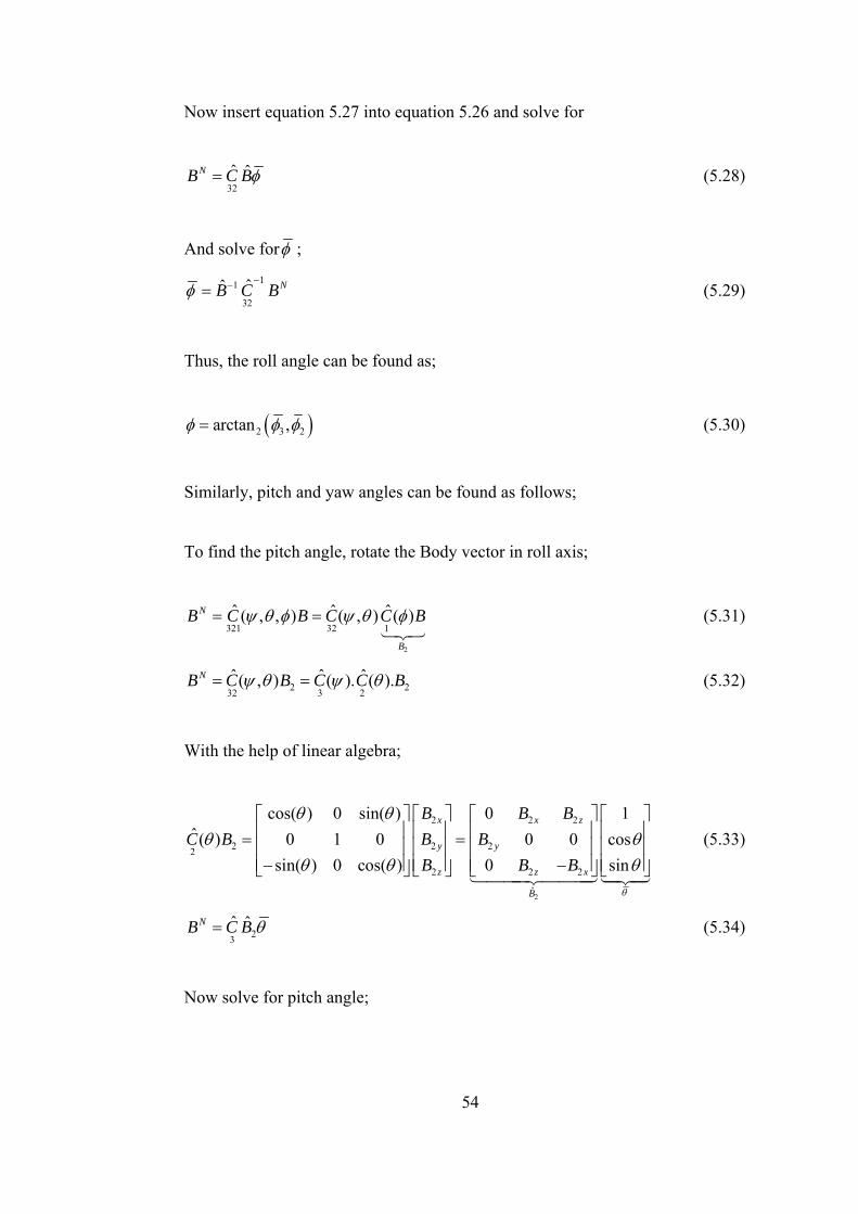
54
Now insert equation 5.27 into equation 5.26 and solve for
32ˆ ˆ=NB C Bφ (5.28)
And solve forφ ;
11
32ˆˆ −−= NB C Bφ (5.29)
Thus, the roll angle can be found as;
( )2 3 2arctan ,φ φ φ= (5.30)
Similarly, pitch and yaw angles can be found as follows;
To find the pitch angle, rotate the Body vector in roll axis;
2
321 32 1ˆ ˆ ˆ( , , ) ( , ) ( )= =N
B
B C B C C Bψ θ φ ψ θ φ (5.31)
2 232 3 2ˆ ˆ ˆ( , ) ( ). ( ).= =NB C B C C Bψ θ ψ θ (5.32)
With the help of linear algebra;
2
2 2 2
2 2 22
2 2 2
ˆ
cos( ) 0 sin( ) 0 1ˆ ( ) 0 1 0 0 0 cos
sin( ) 0 cos( ) 0 sin
x x z
y y
z z x
B
B B BC B B B
B B Bθ
θ θθ θ
θ θ θ
⎡ ⎤ ⎡ ⎤ ⎡ ⎤ ⎡ ⎤⎢ ⎥ ⎢ ⎥ ⎢ ⎥ ⎢ ⎥= =⎢ ⎥ ⎢ ⎥ ⎢ ⎥ ⎢ ⎥⎢ ⎥ ⎢ ⎥ ⎢ ⎥ ⎢ ⎥− −⎣ ⎦ ⎣ ⎦ ⎣ ⎦ ⎣ ⎦
(5.33)
23ˆ ˆ=NB C B θ (5.34)
Now solve for pitch angle;
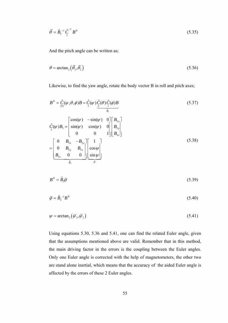
55
112 3
ˆˆ −−= NB C Bθ (5.35)
And the pitch angle can be written as;
( )2 3 2arctan ,θ θ θ= (5.36)
Likewise, to find the yaw angle, rotate the body vector B in roll and pitch axes;
3
321 3 2 1ˆ ˆ ˆ ˆ( , , ) ( ) ( ) ( )= =N
B
B C B C C C Bψ θ φ ψ θ φ (5.37)
3
3
3 33
3
3 3
3 3
3
ˆ
cos( ) sin( ) 0ˆ ( ) sin( ) cos( ) 0
0 0 1
0 10 cos
0 0 sin
−⎡ ⎤ ⎡ ⎤⎢ ⎥ ⎢ ⎥= ⎢ ⎥ ⎢ ⎥⎢ ⎥ ⎢ ⎥⎣ ⎦ ⎣ ⎦
−⎡ ⎤ ⎡ ⎤⎢ ⎥ ⎢ ⎥= ⎢ ⎥ ⎢ ⎥⎢ ⎥ ⎢ ⎥⎣ ⎦ ⎣ ⎦
x
y
z
x y
y x
z
B
BC B B
B
B BB B
Bϕ
ψ ψψ ψ ψ
ψψ
(5.38)
3ˆ=NB B ϕ (5.39)
1
2ˆ −= NB Bϕ (5.40)
( )2 3 2arctan ,=ψ ψ ψ (5.41)
Using equations 5.30, 5.36 and 5.41, one can find the related Euler angle, given
that the assumptions mentioned above are valid. Remember that in this method,
the main driving factor in the errors is the coupling between the Euler angles.
Only one Euler angle is corrected with the help of magnetometers, the other two
are stand alone inertial, which means that the accuracy of the aided Euler angle is
affected by the errors of these 2 Euler angles.

56
As this method is an analytical solution, it is not accurate as the Kalman filtered
solution. Besides, the cumulative error in the unaided Euler angles will result in
high errors in the aided Euler angle. This method can be used only in a short
period of time. The main advantage of this algorithm is its computational
superiority over Kalman filtered solution.
57
CHAPTER 6
6 GROUND ALIGNMENT VIA MEMS IMU +
MAGNETOMETER
In a high accuracy IMU, it is possible to align the navigation system by using the
inertial measurements, which is also known as self alignment or quasi stationary
alignment. This method is generally composed of two main parts [36, 37, and 38];
1. Coarse Alignment
2. Fine Alignment
Where coarse alignment is an analytical solution and the fine alignment is the part
that the Kalman filter is used.
The reason for this partition is arising from the nature of estimation algorithms. In
most of the navigation system, Kalman filter is used, which is indeed a linear
estimation filter. As explained in the previous chapters, the states in the estimation
are the navigation and sensor errors. The navigation error equations were derived
by using the small attitude error assumption, which is valid up to 20 degree errors.
[1, 11, 13, 14]
58
The coarse alignment phase is an analytic procedure, in which two sets of vector
equations are used to find the related direction cosine matrix. In a high accuracy
system, gravity and earth rotation rate is used as the vector equations. As it is
implied in its name, the solution is “coarse”, that is accuracy is only up to 1-0.5
degrees. The main function of the coarse alignment phase is to make the attitude
errors as small as possible so that the linearity assumption in the navigation errors
is valid. The details of the coarse alignment process were given in the previous
chapter.
The fine alignment phase is the part where not only the attitude errors are found
with high accuracy, but also the sensor errors may be estimated. In the fine
alignment process, following measurements are taken into consideration;
1. Two sets of vector equations
2. Zero velocity
3. Constant Position
As explained above, the ground alignment algorithms use earth rotation rate (~15
deg/hr) and gravity (~9.801 m/s2) as the vector measurement equations. MEMS
accelerometers generally have a bias repeatability in the order of 10 mg, thus they
can measure the gravitational acceleration accurate enough such that it may be
used as a vector equation. On the other hand, MEMS gyros have a drift
repeatability in the order of 100 deg/hr, which is greatly higher than the earth
rotation rate. Earth rotation rate can not be used as a vector measurement where
MEMS gyros are used.
In the proposed method, the magnetic field is used as a vector measurement
equation. The MEMS magnetometers have high accuracy, and the reference
magnetic field (world magnetic field) can be modeled very accurately.
The simulations are carried out in Matlab®. The structure of the simulation
environment is given as follows;
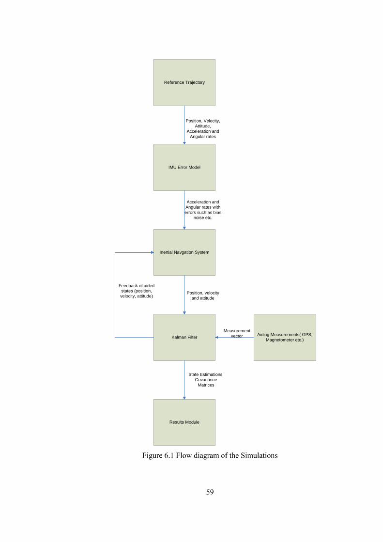
59
Reference Trajectory
Position, Velocity,Attitude,
Acceleration and Angular rates
IMU Error Model
Inertial Navgation System
Aiding Measurements( GPS, Magnetometer etc.)Kalman Filter
Acceleration and Angular rates with errors such as bias
noise etc.
Measurement vector
Position, velocity and attitude
Feedback of aided states (position, velocity, attitude)
Results Module
State Estimations, Covariance
Matrices
Figure 6.1 Flow diagram of the Simulations

60
The Matlab®. codes that developed in this thesis are given in Appendix F.
6.1 Coarse Alignment
In the coarse alignment procedure, Equations (5.1)-(5.5) are used, where the
gravity and magnetic field are used as vector measurements.
6.1.1 Monte Carlo Simulations
In the simulation and experimental studies process, the following sensor sets are
used;
• Colibrys MS8000.C Accelerometer
• Inertial Science RRS01 Gyro
• HMC 1053 Magnetometer
Performance specifications of these sensors are given in the Appendix.
In the Monte Carlo Simulations, following set of random variables is used;
• Gyro Bias Repeatability : 100 deg/hr (1 σ), Normal Distribution
• Gyro Noise: 1 deg/s (1 σ), Normal Distribution
• Gyro Scale Factor Error: 1000 ppm (1 σ), Normal Distribution
• Accelerometer Bias Repeatability 10 mg (1 σ),: Normal Distribution
• Accelerometer Noise : 5 mg (1 σ), Normal Distribution
• Accelerometer Scale Factor Error: 1000 ppm (1 σ), Normal Distribution
• Magnetometer Noise: 5 mGauss (1 σ), Normal Distribution
• Attitude of the Sensor Block (North, East, Down) : Uniform Distribution
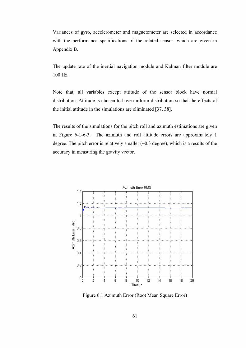
61
Variances of gyro, accelerometer and magnetometer are selected in accordance
with the performance specifications of the related sensor, which are given in
Appendix B.
The update rate of the inertial navigation module and Kalman filter module are
100 Hz.
Note that, all variables except attitude of the sensor block have normal
distribution. Attitude is chosen to have uniform distribution so that the effects of
the initial attitude in the simulations are eliminated [37, 38].
The results of the simulations for the pitch roll and azimuth estimations are given
in Figure 6-1-6-3. The azimuth and roll attitude errors are approximately 1
degree. The pitch error is relatively smaller (~0.3 degree), which is a results of the
accuracy in measuring the gravity vector.
Figure 6.1 Azimuth Error (Root Mean Square Error)
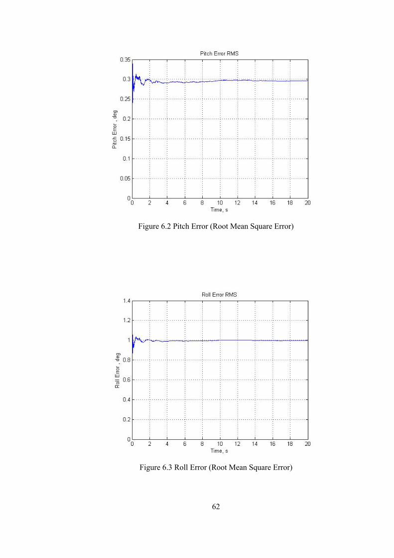
62
Figure 6.2 Pitch Error (Root Mean Square Error)
Figure 6.3 Roll Error (Root Mean Square Error)
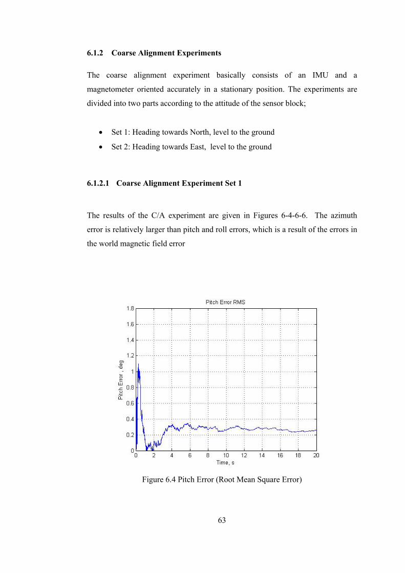
63
6.1.2 Coarse Alignment Experiments
The coarse alignment experiment basically consists of an IMU and a
magnetometer oriented accurately in a stationary position. The experiments are
divided into two parts according to the attitude of the sensor block;
• Set 1: Heading towards North, level to the ground
• Set 2: Heading towards East, level to the ground
6.1.2.1 Coarse Alignment Experiment Set 1
The results of the C/A experiment are given in Figures 6-4-6-6. The azimuth
error is relatively larger than pitch and roll errors, which is a result of the errors in
the world magnetic field error
Figure 6.4 Pitch Error (Root Mean Square Error)
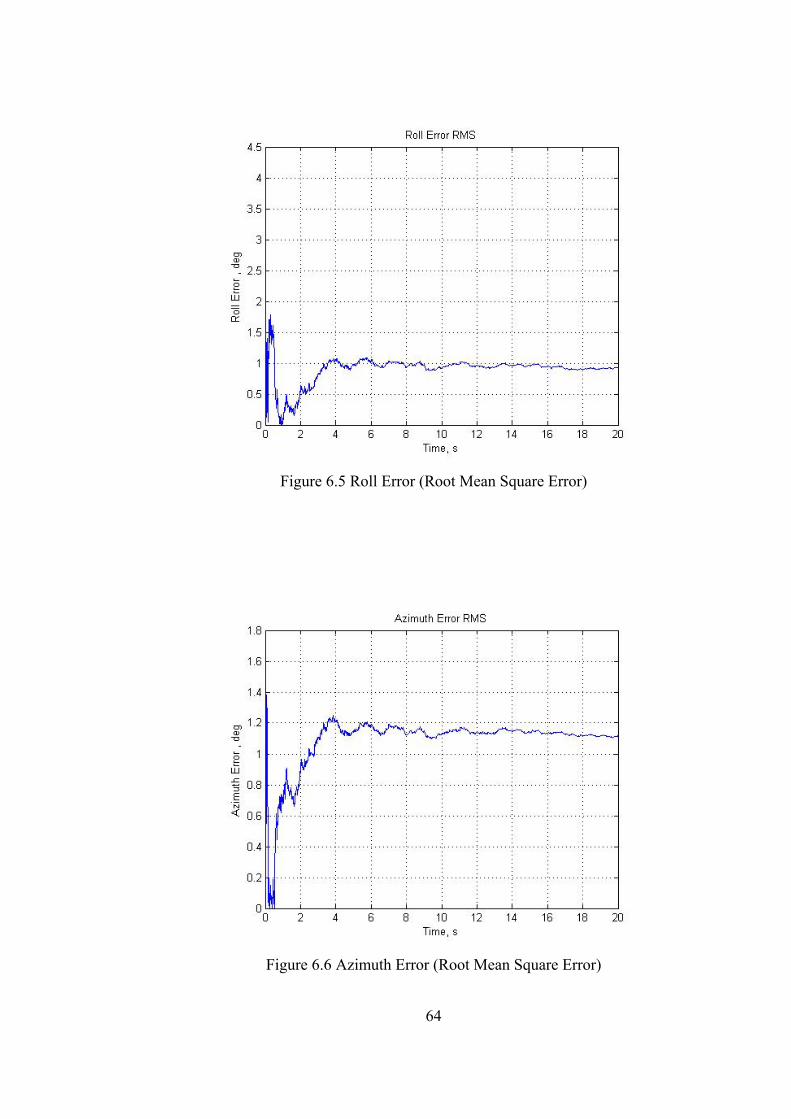
64
Figure 6.5 Roll Error (Root Mean Square Error)
Figure 6.6 Azimuth Error (Root Mean Square Error)
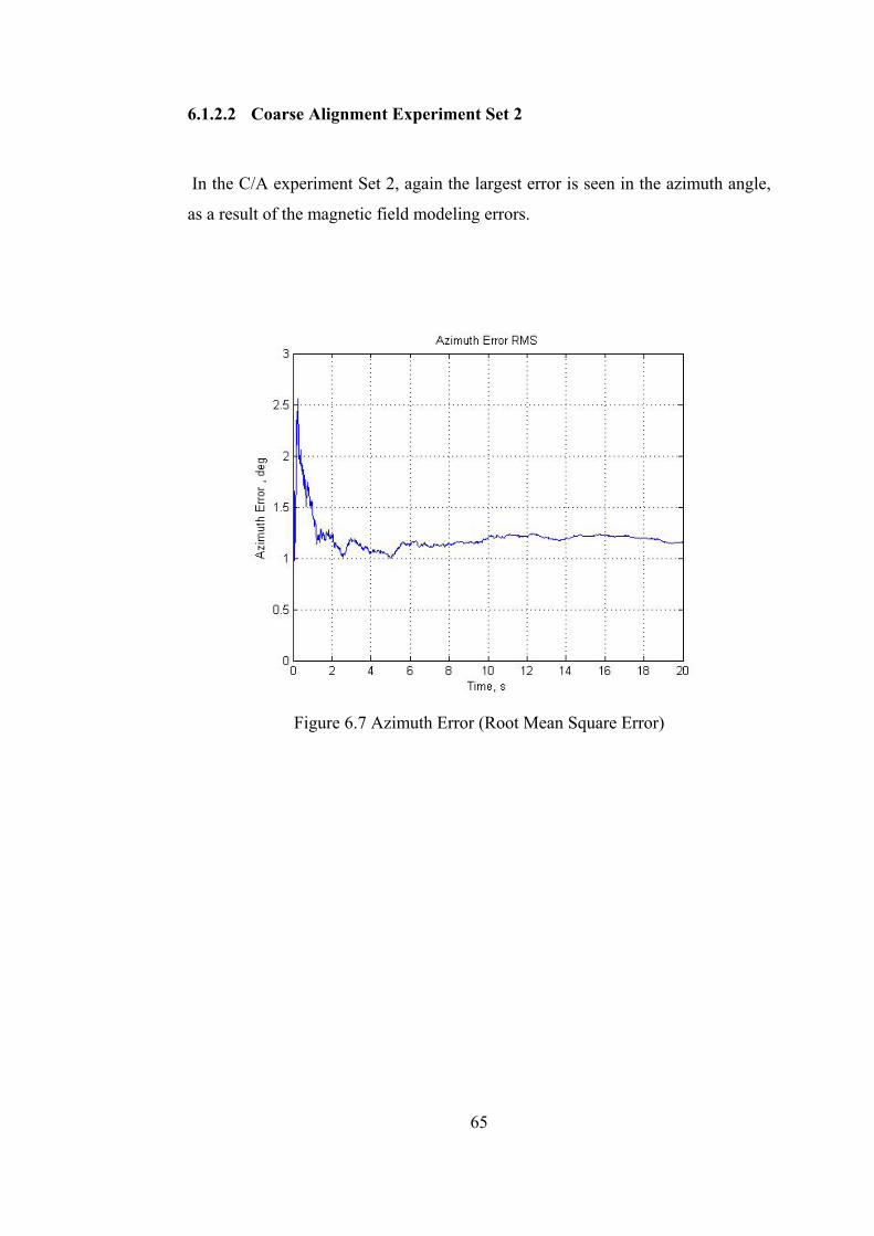
65
6.1.2.2 Coarse Alignment Experiment Set 2
In the C/A experiment Set 2, again the largest error is seen in the azimuth angle,
as a result of the magnetic field modeling errors.
Figure 6.7 Azimuth Error (Root Mean Square Error)
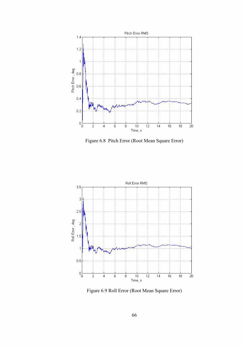
66
Figure 6.8 Pitch Error (Root Mean Square Error)
Figure 6.9 Roll Error (Root Mean Square Error)

67
6.2 Fine Alignment
The fine alignment algorithm is in fact a stochastic estimation. The estimation
filter is a linear Kalman filter. As the navigation unit is stationary through the
alignment, GPS velocity (quasi stationary velocity) and position (constant
position) measurements are used in addition to the accelerometer and
magnetometer measurements,
6.2.1 Monte Carlo Simulations
The states of the Kalman filter are;
• 3 states of attitude error
• 3 states of velocity error
• 3 states of position error
• 3 states of gyro bias
• 3 states of accelerometer bias
The attitude, velocity and position errors are modeled with equations given in
Chapter 2, where gyro and accelerometer noises are modeled as random constants.
The scale factor error, misalignment errors etc. are not modeled in the estimation
filter as these errors are not observable in the MEMS sensors.
The process noises are;
• Accelerometer noises
• Gyro noises
The measurements are;
• Accelerometer measurements
• Magnetometer measurements
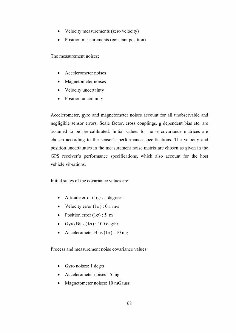
68
• Velocity measurements (zero velocity)
• Position measurements (constant position)
The measurement noises;
• Accelerometer noises
• Magnetometer noises
• Velocity uncertainty
• Position uncertainty
Accelerometer, gyro and magnetometer noises account for all unobservable and
negligible sensor errors. Scale factor, cross couplings, g dependent bias etc. are
assumed to be pre-calibrated. Initial values for noise covariance matrices are
chosen according to the sensor’s performance specifications. The velocity and
position uncertainties in the measurement noise matrix are chosen as given in the
GPS receiver’s performance specifications, which also account for the host
vehicle vibrations.
Initial states of the covariance values are;
• Attitude error (1σ) : 5 degrees
• Velocity error (1σ) : 0.1 m/s
• Position error (1σ) : 5 m
• Gyro Bias (1σ) : 100 deg/hr
• Accelerometer Bias (1σ) : 10 mg
Process and measurement noise covariance values:
• Gyro noises: 1 deg/s
• Accelerometer noises : 5 mg
• Magnetometer noises: 10 mGauss

69
• Velocity uncertainty: 0.1 m/s
• Position uncertainty: 5 m
The random variables in the Monte Carlo Simulations are as follows,
• Gyro Bias Repeatability : 100 deg/hr (1 σ), Normal Distribution
• Gyro Noise: 1 deg/s (1 σ), Normal Distribution
• Gyro Scale Factor Error: 1000 ppm (1 σ), Normal Distribution
• Accelerometer Bias Repeatability 10 mg (1 σ), Normal Distribution
• Accelerometer Noise : 5 mg (1 σ), Normal Distribution
• Accelerometer Scale Factor Error: 1000 ppm (1 σ), Normal Distribution
• Magnetometer Noise: 5 mgauss (1 σ), Normal Distribution
• Attitude of the Sensor Block (North, East, Down) : Uniform Distribution
• Velocity uncertainty: 0.1 m/s, (1 σ), Normal Distribution
• Position uncertainty: 5 m, (1 σ), Normal Distribution
The gyro, accelerometer and magnetometer variances are chosen in accordance
with their performance specification, given in Appendix B
The primary objective of the fine alignment algorithm is to find the attitude angles
in a high accuracy, which can be seen in Figure 6.10-6.12. The secondary
objective is to on-line calibrate the IMU. The designed algorithm can estimate the
bias errors of the accelerometer and gyros in a fast and accurate manner (Figures
6-10-6-18)
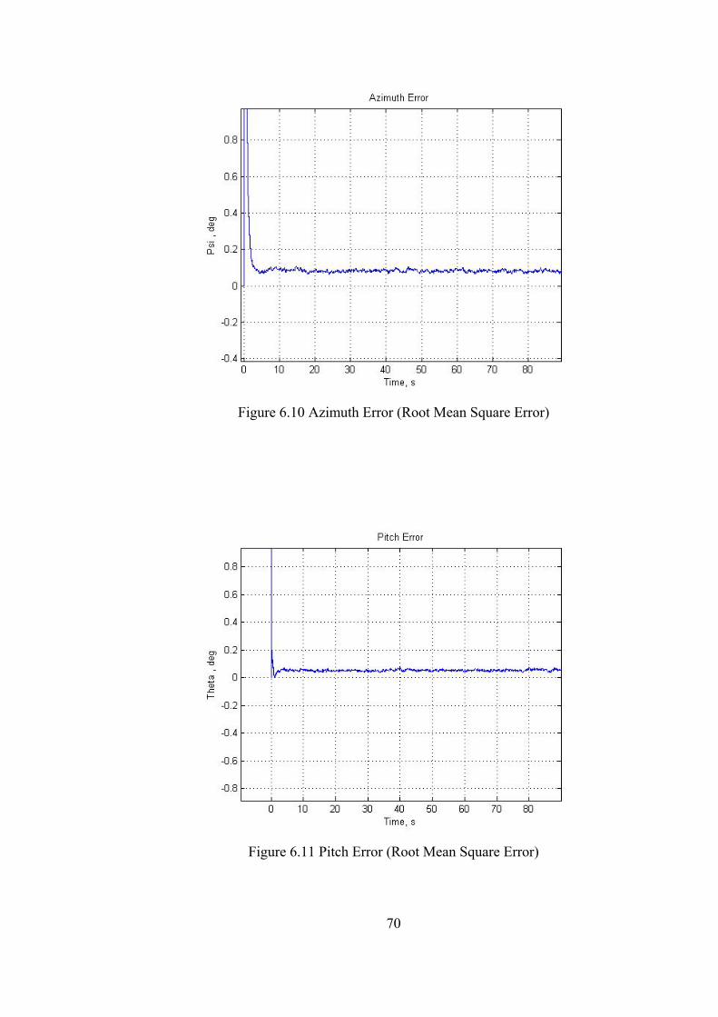
70
Figure 6.10 Azimuth Error (Root Mean Square Error)
Figure 6.11 Pitch Error (Root Mean Square Error)
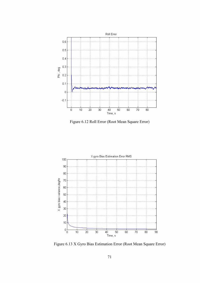
71
Figure 6.12 Roll Error (Root Mean Square Error)
Figure 6.13 X Gyro Bias Estimation Error (Root Mean Square Error)
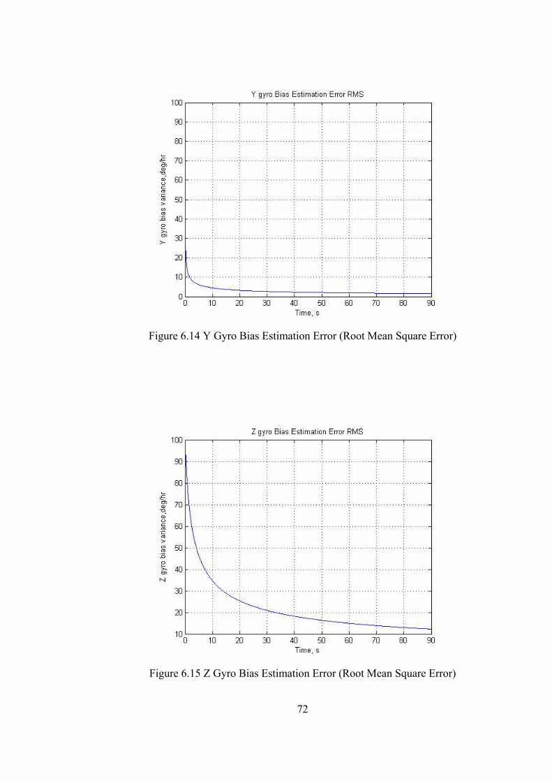
72
Figure 6.14 Y Gyro Bias Estimation Error (Root Mean Square Error)
Figure 6.15 Z Gyro Bias Estimation Error (Root Mean Square Error)
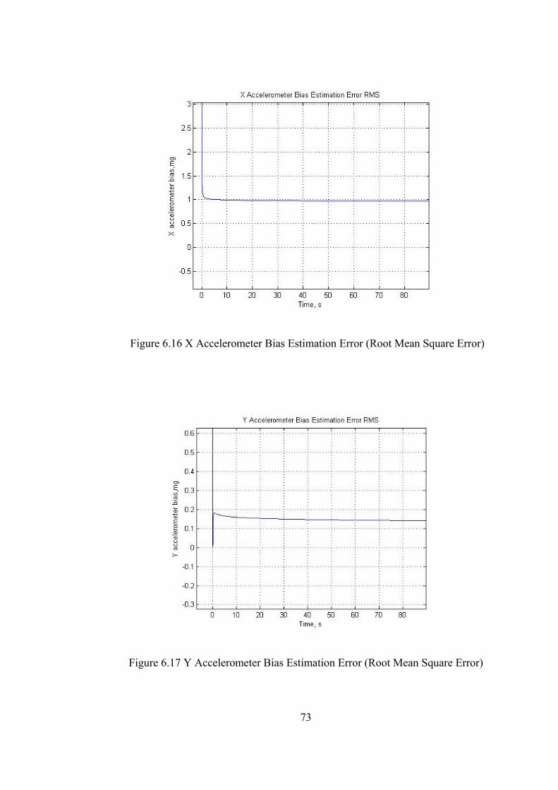
73
Figure 6.16 X Accelerometer Bias Estimation Error (Root Mean Square Error)
Figure 6.17 Y Accelerometer Bias Estimation Error (Root Mean Square Error)
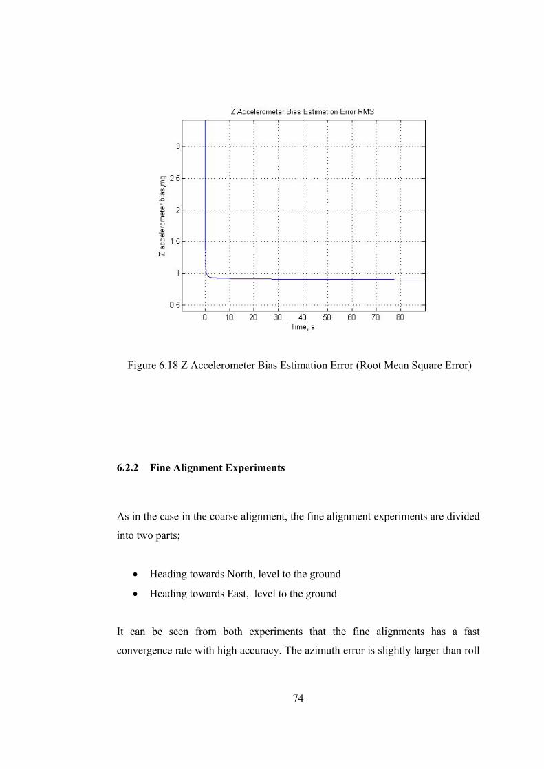
74
Figure 6.18 Z Accelerometer Bias Estimation Error (Root Mean Square Error)
6.2.2 Fine Alignment Experiments
As in the case in the coarse alignment, the fine alignment experiments are divided
into two parts;
• Heading towards North, level to the ground
• Heading towards East, level to the ground
It can be seen from both experiments that the fine alignments has a fast
convergence rate with high accuracy. The azimuth error is slightly larger than roll
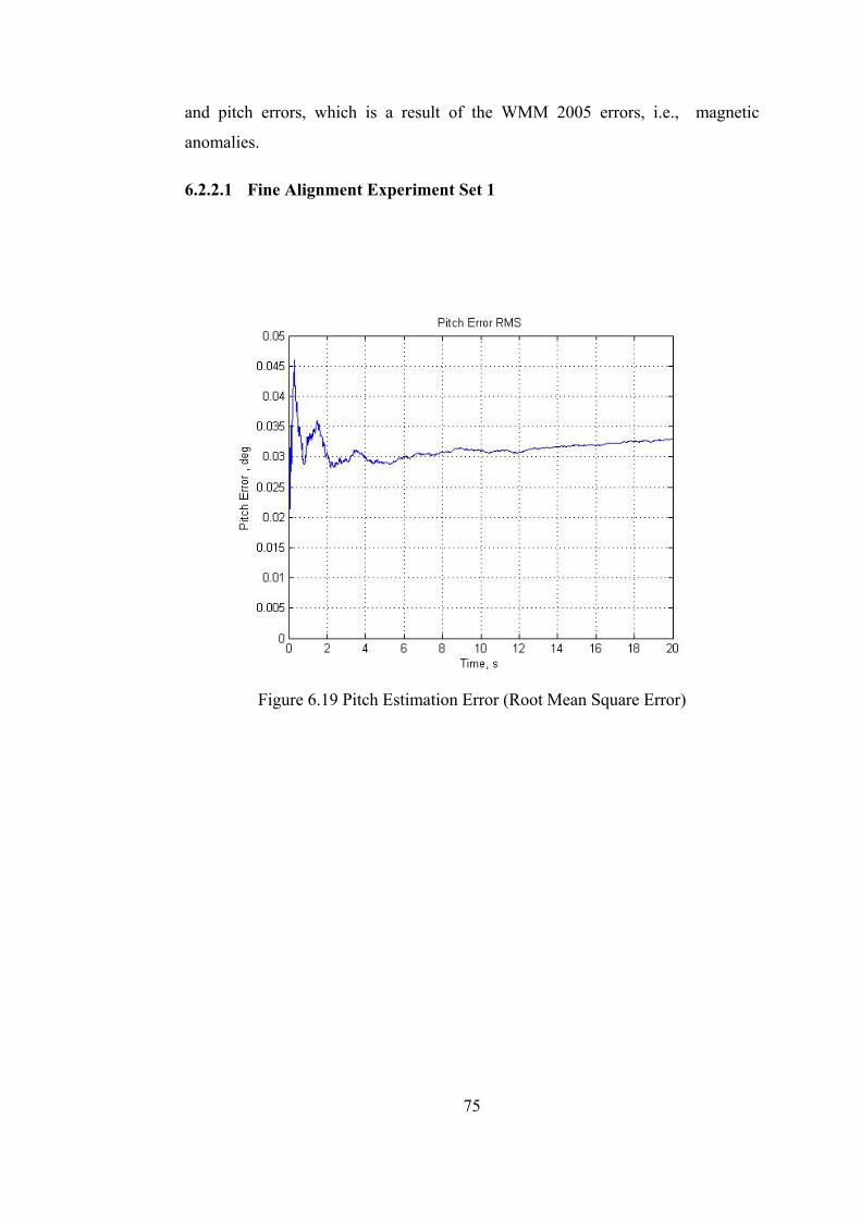
75
and pitch errors, which is a result of the WMM 2005 errors, i.e., magnetic
anomalies.
6.2.2.1 Fine Alignment Experiment Set 1
Figure 6.19 Pitch Estimation Error (Root Mean Square Error)
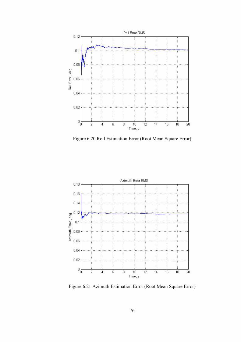
76
Figure 6.20 Roll Estimation Error (Root Mean Square Error)
Figure 6.21 Azimuth Estimation Error (Root Mean Square Error)
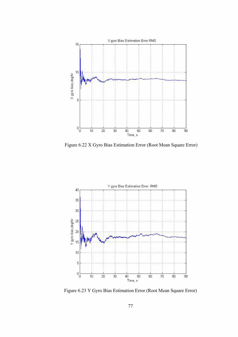
77
Figure 6.22 X Gyro Bias Estimation Error (Root Mean Square Error)
Figure 6.23 Y Gyro Bias Estimation Error (Root Mean Square Error)
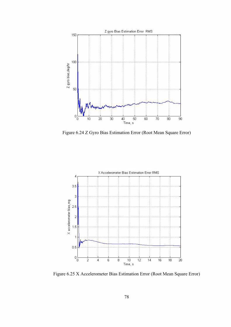
78
Figure 6.24 Z Gyro Bias Estimation Error (Root Mean Square Error)
Figure 6.25 X Accelerometer Bias Estimation Error (Root Mean Square Error)
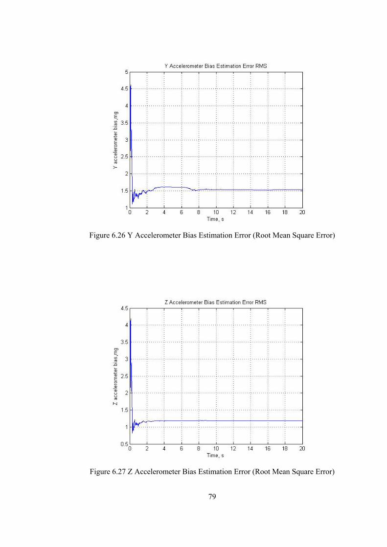
79
Figure 6.26 Y Accelerometer Bias Estimation Error (Root Mean Square Error)
Figure 6.27 Z Accelerometer Bias Estimation Error (Root Mean Square Error)
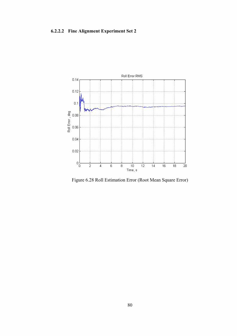
80
6.2.2.2 Fine Alignment Experiment Set 2
Figure 6.28 Roll Estimation Error (Root Mean Square Error)
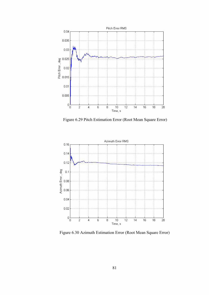
81
Figure 6.29 Pitch Estimation Error (Root Mean Square Error)
Figure 6.30 Azimuth Estimation Error (Root Mean Square Error)
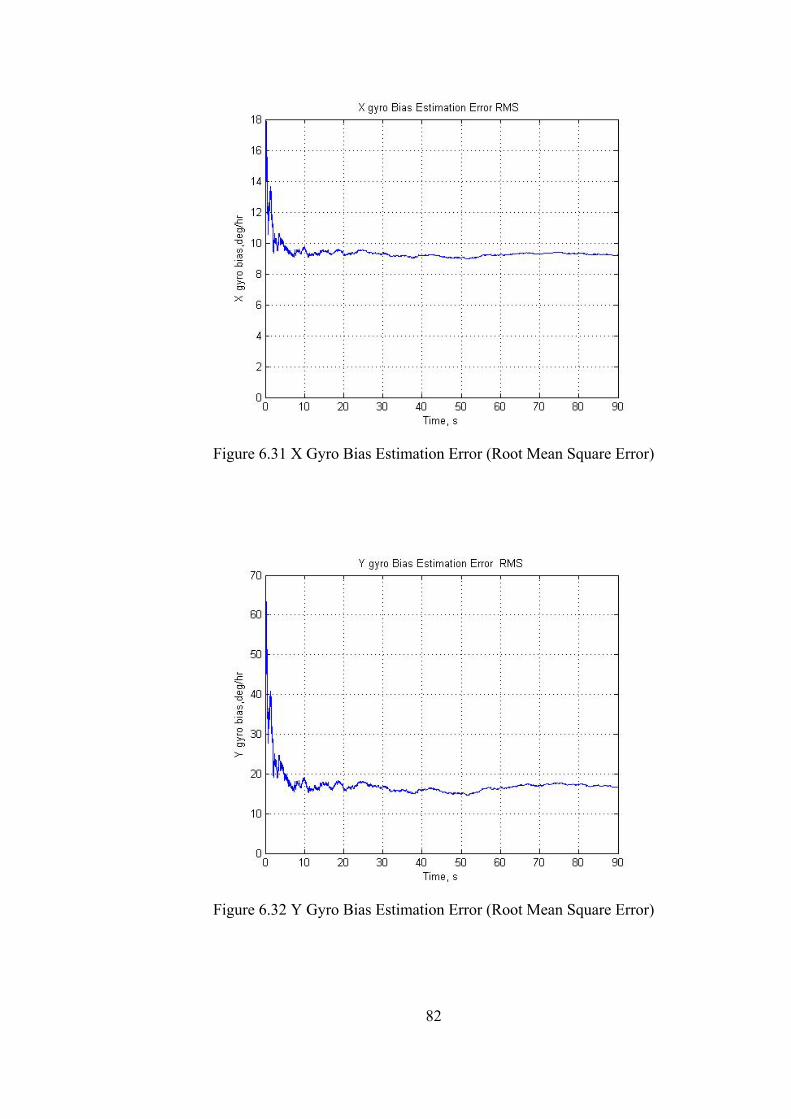
82
Figure 6.31 X Gyro Bias Estimation Error (Root Mean Square Error)
Figure 6.32 Y Gyro Bias Estimation Error (Root Mean Square Error)
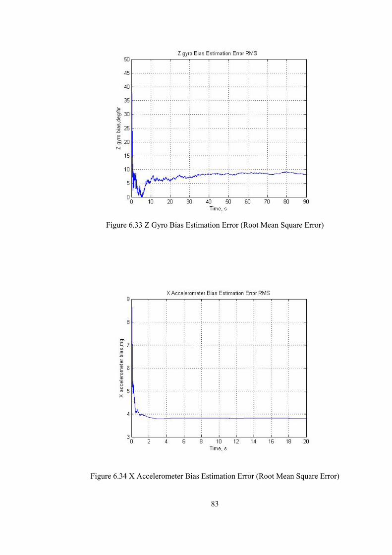
83
Figure 6.33 Z Gyro Bias Estimation Error (Root Mean Square Error)
Figure 6.34 X Accelerometer Bias Estimation Error (Root Mean Square Error)
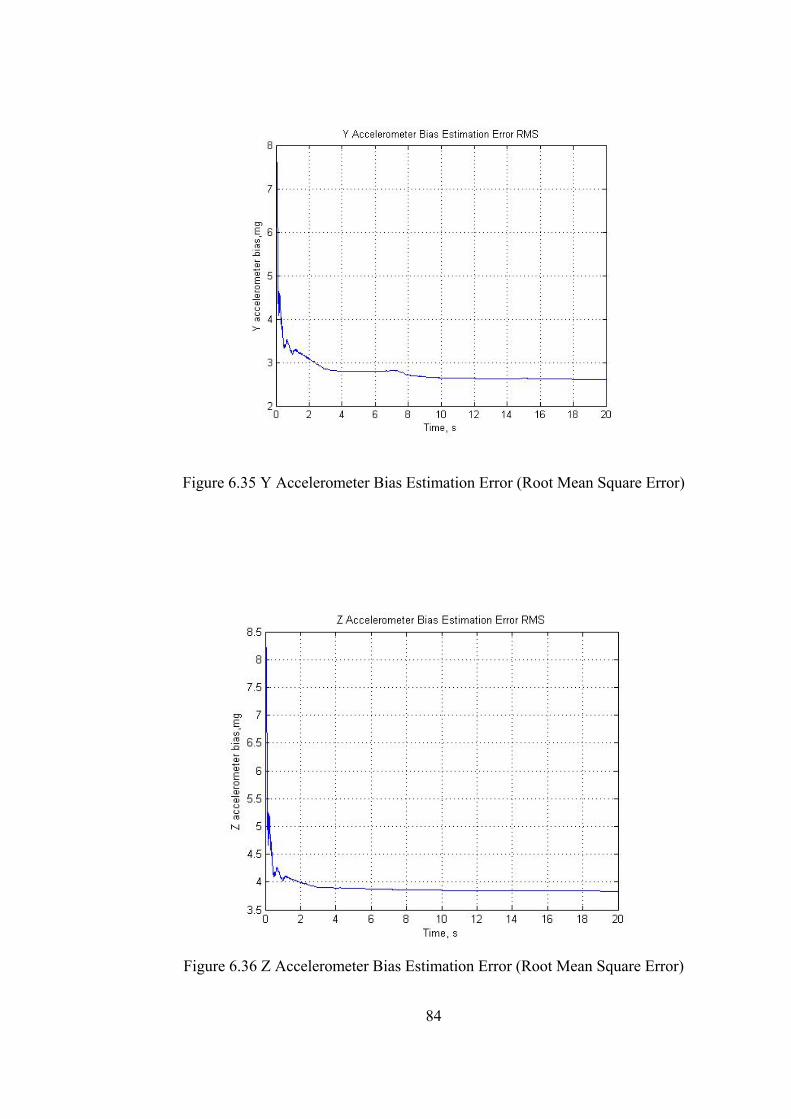
84
Figure 6.35 Y Accelerometer Bias Estimation Error (Root Mean Square Error)
Figure 6.36 Z Accelerometer Bias Estimation Error (Root Mean Square Error)
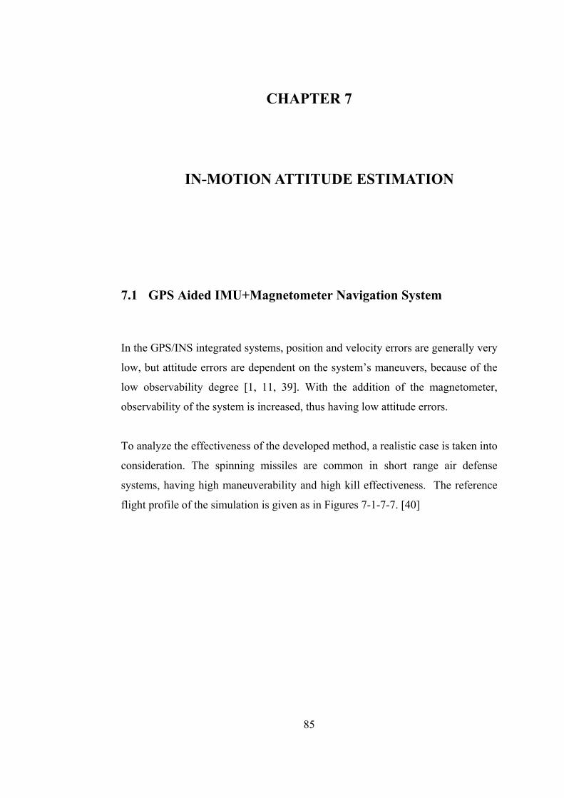
85
CHAPTER 7
7 IN-MOTION ATTITUDE ESTIMATION
7.1 GPS Aided IMU+Magnetometer Navigation System
In the GPS/INS integrated systems, position and velocity errors are generally very
low, but attitude errors are dependent on the system’s maneuvers, because of the
low observability degree [1, 11, 39]. With the addition of the magnetometer,
observability of the system is increased, thus having low attitude errors.
To analyze the effectiveness of the developed method, a realistic case is taken into
consideration. The spinning missiles are common in short range air defense
systems, having high maneuverability and high kill effectiveness. The reference
flight profile of the simulation is given as in Figures 7-1-7-7. [40]
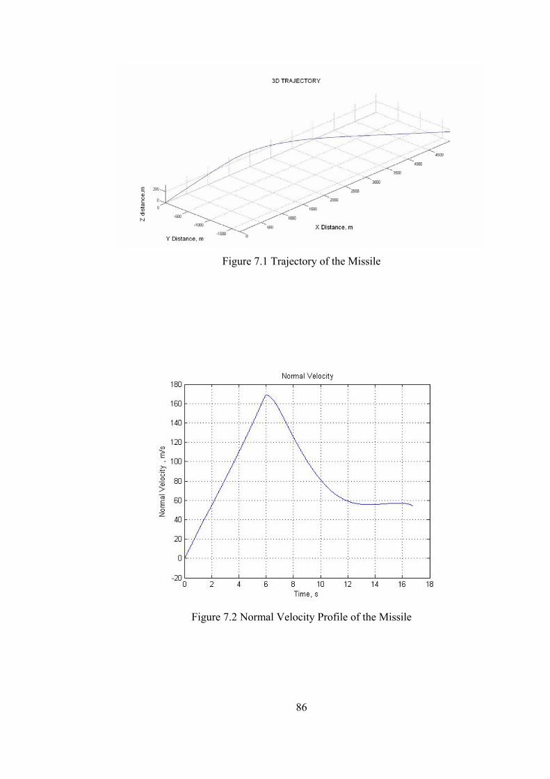
86
Figure 7.1 Trajectory of the Missile
Figure 7.2 Normal Velocity Profile of the Missile
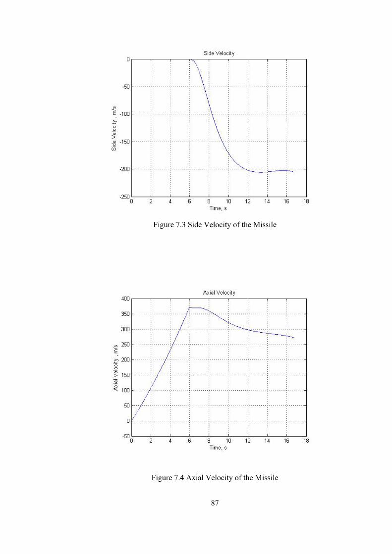
87
Figure 7.3 Side Velocity of the Missile
Figure 7.4 Axial Velocity of the Missile
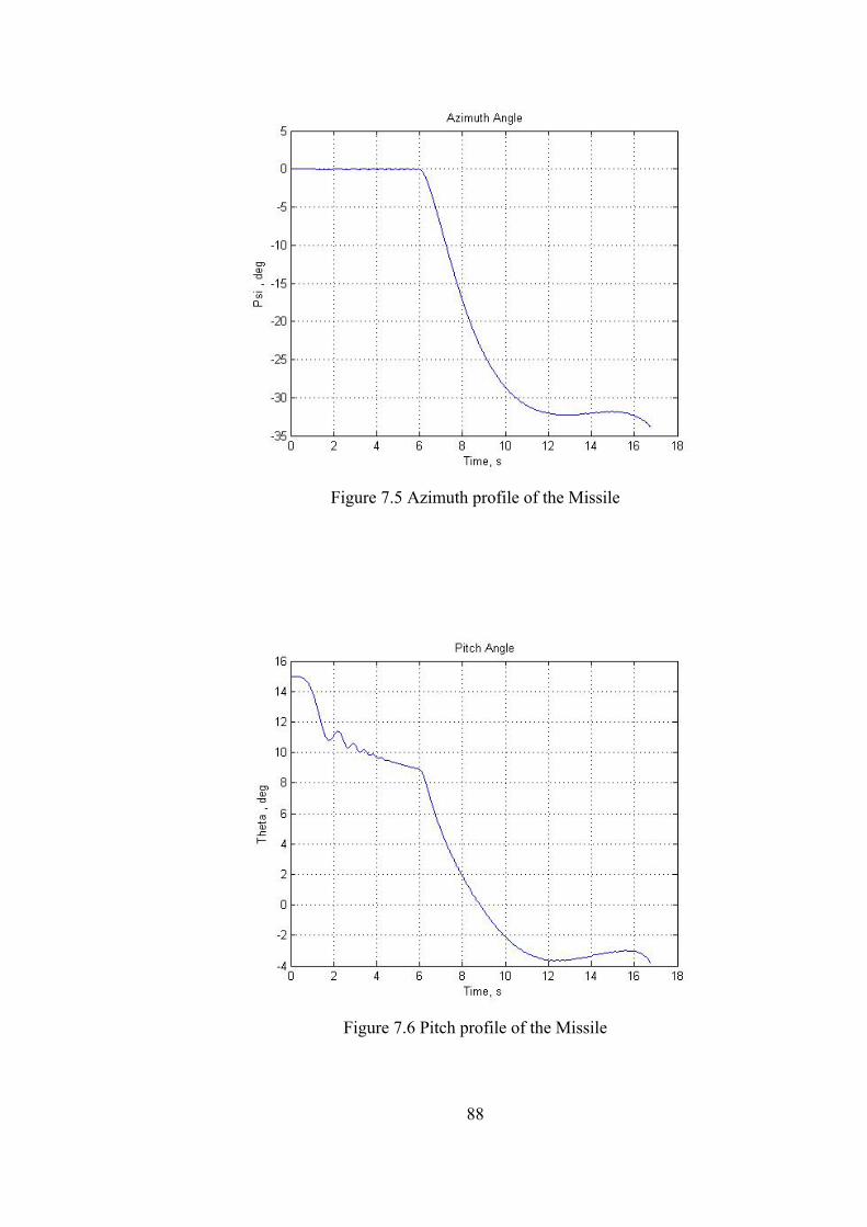
88
Figure 7.5 Azimuth profile of the Missile
Figure 7.6 Pitch profile of the Missile
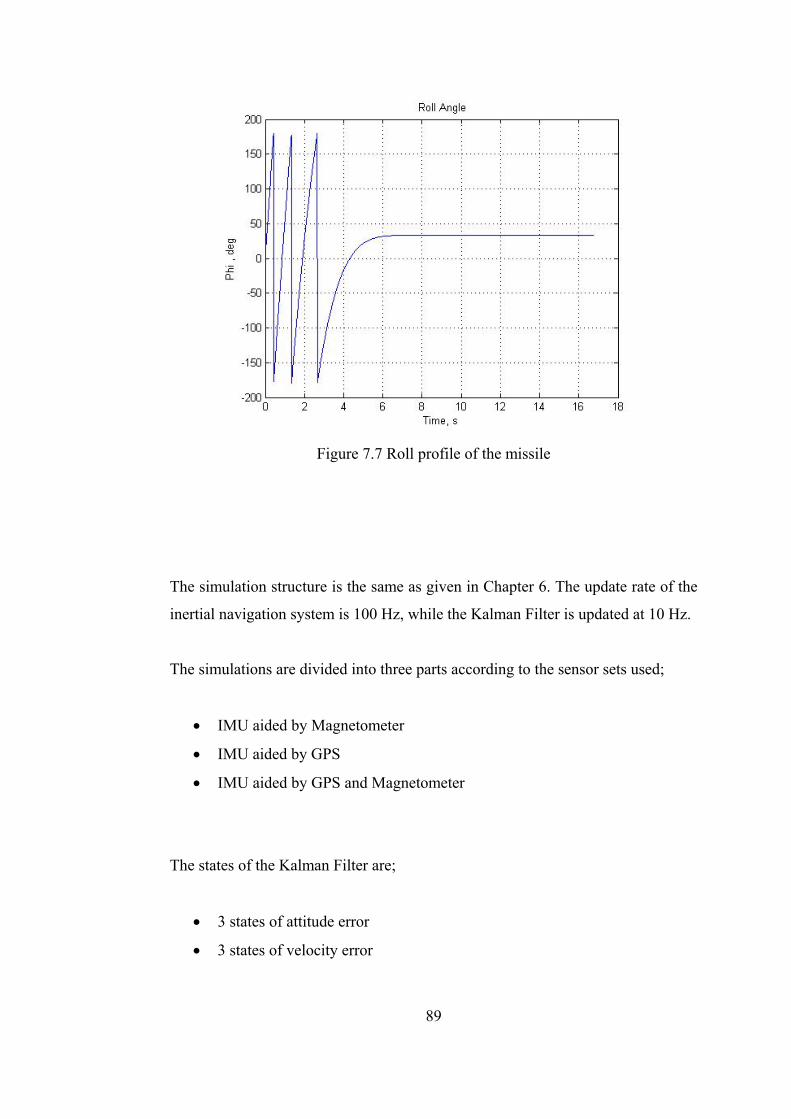
89
Figure 7.7 Roll profile of the missile
The simulation structure is the same as given in Chapter 6. The update rate of the
inertial navigation system is 100 Hz, while the Kalman Filter is updated at 10 Hz.
The simulations are divided into three parts according to the sensor sets used;
• IMU aided by Magnetometer
• IMU aided by GPS
• IMU aided by GPS and Magnetometer
The states of the Kalman Filter are;
• 3 states of attitude error
• 3 states of velocity error
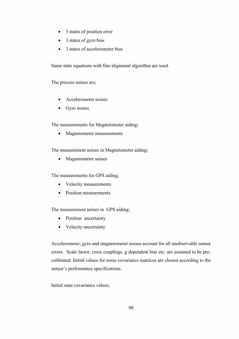
90
• 3 states of position error
• 3 states of gyro bias
• 3 states of accelerometer bias
Same state equations with fine alignment algorithm are used.
The process noises are;
• Accelerometer noises
• Gyro noises
The measurements for Magnetometer aiding;
• Magnetometer measurements
The measurement noises in Magnetometer aiding;
• Magnetometer noises
The measurements for GPS aiding;
• Velocity measurements
• Position measurements
The measurement noises in GPS aiding;
• Position uncertainty
• Velocity uncertainty
Accelerometer, gyro and magnetometer noises account for all unobservable sensor
errors. Scale factor, cross couplings, g dependent bias etc. are assumed to be pre-
calibrated. Initial values for noise covariance matrices are chosen according to the
sensor’s performance specifications.
Initial state covariance values;

91
• Attitude error (1σ) : 5 degrees
• Velocity error (1σ) : 0.1 m/s
• Position error (1σ) : 0.1 m
• Gyro Bias (1σ) : 100 deg/hr
• Accelerometer Bias (1σ) : 10 mg
Noise covariance values:
• Gyro noises: 1 deg/s
• Accelerometer noises : 5 mg
• Magnetometer noises: 10 mGauss
• Velocity uncertainty: 0.1 m/s
• Position uncertainty: 5 m
The random variables in the Monte Carlo Simulations are as follows,
• Gyro Bias Repeatability : 100 deg/hr (1 σ), Normal Distribution
• Gyro Noise: 1 deg/s (1 σ), Normal Distribution
• Gyro Scale Factor Error: 1000 ppm (1 σ), Normal Distribution
• Accelerometer Bias Repeatability 10 mg (1 σ), Normal Distribution
• Accelerometer Noise : 5 mg (1 σ), Normal Distribution
• Accelerometer Scale Factor Error: 1000 ppm (1 σ), Normal Distribution
• Magnetometer Noise: 5 mgauss (1 σ), Normal Distribution
• Attitude of the Sensor Block (North, East, Down) : Uniform Distribution
• Velocity uncertainty: 0.1 m/s, (1 σ), Normal Distribution
• Position uncertainty: 5 m, (1 σ), Normal Distribution
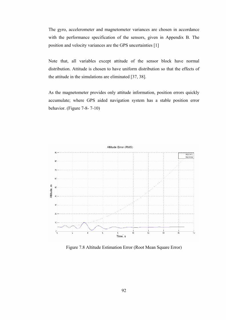
92
The gyro, accelerometer and magnetometer variances are chosen in accordance
with the performance specification of the sensors, given in Appendix B. The
position and velocity variances are the GPS uncertainties [1]
Note that, all variables except attitude of the sensor block have normal
distribution. Attitude is chosen to have uniform distribution so that the effects of
the attitude in the simulations are eliminated [37, 38].
As the magnetometer provides only attitude information, position errors quickly
accumulate; where GPS aided navigation system has a stable position error
behavior. (Figure 7-8- 7-10)
Figure 7.8 Altitude Estimation Error (Root Mean Square Error)
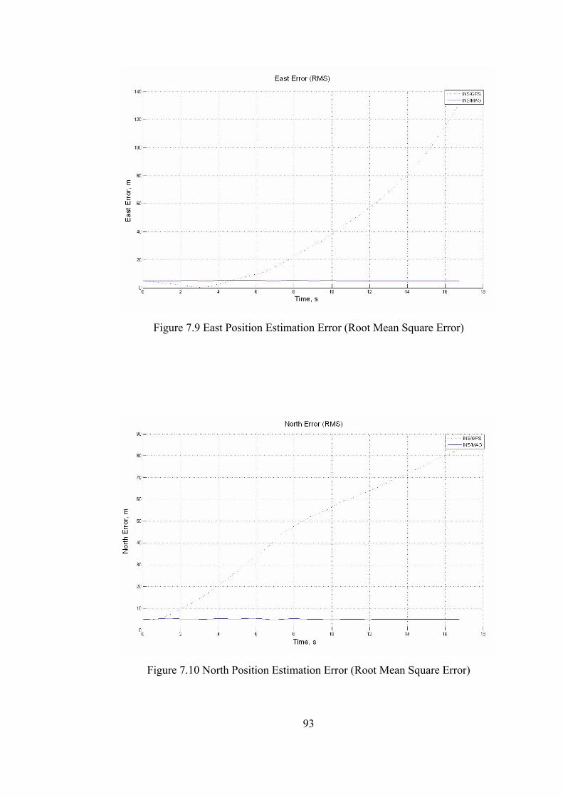
93
Figure 7.9 East Position Estimation Error (Root Mean Square Error)
Figure 7.10 North Position Estimation Error (Root Mean Square Error)
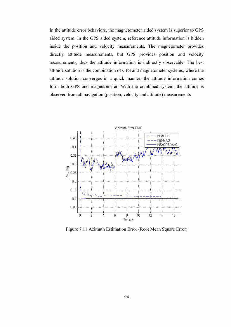
94
In the attitude error behaviors, the magnetometer aided system is superior to GPS
aided system. In the GPS aided system, reference attitude information is hidden
inside the position and velocity measurements. The magnetometer provides
directly attitude measurements, but GPS provides position and velocity
measurements, thus the attitude information is indirectly observable. The best
attitude solution is the combination of GPS and magnetometer systems, where the
attitude solution converges in a quick manner; the attitude information comes
form both GPS and magnetometer. With the combined system, the attitude is
observed from all navigation (position, velocity and attitude) measurements
Figure 7.11 Azimuth Estimation Error (Root Mean Square Error)
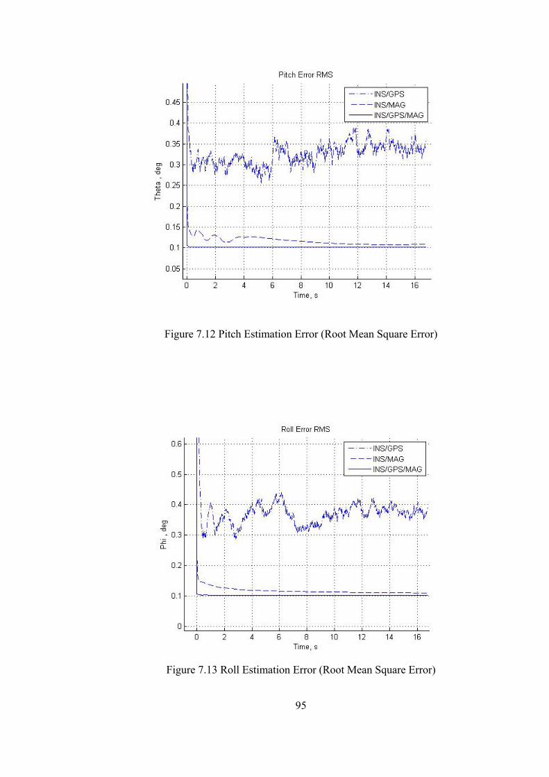
95
Figure 7.12 Pitch Estimation Error (Root Mean Square Error)
Figure 7.13 Roll Estimation Error (Root Mean Square Error)
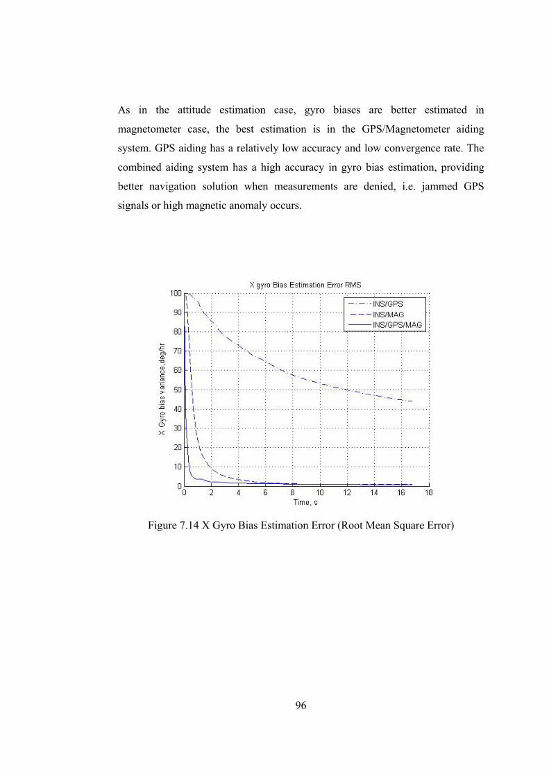
96
As in the attitude estimation case, gyro biases are better estimated in
magnetometer case, the best estimation is in the GPS/Magnetometer aiding
system. GPS aiding has a relatively low accuracy and low convergence rate. The
combined aiding system has a high accuracy in gyro bias estimation, providing
better navigation solution when measurements are denied, i.e. jammed GPS
signals or high magnetic anomaly occurs.
Figure 7.14 X Gyro Bias Estimation Error (Root Mean Square Error)
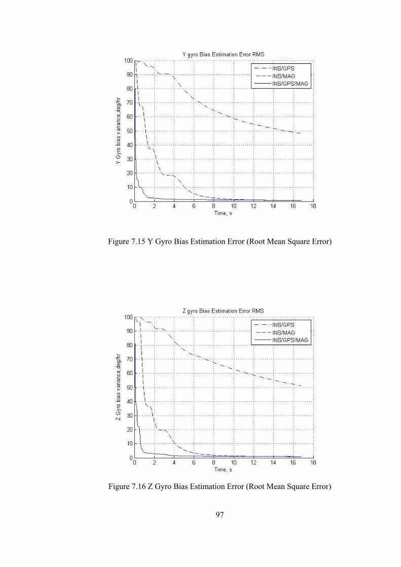
97
Figure 7.15 Y Gyro Bias Estimation Error (Root Mean Square Error)
Figure 7.16 Z Gyro Bias Estimation Error (Root Mean Square Error)
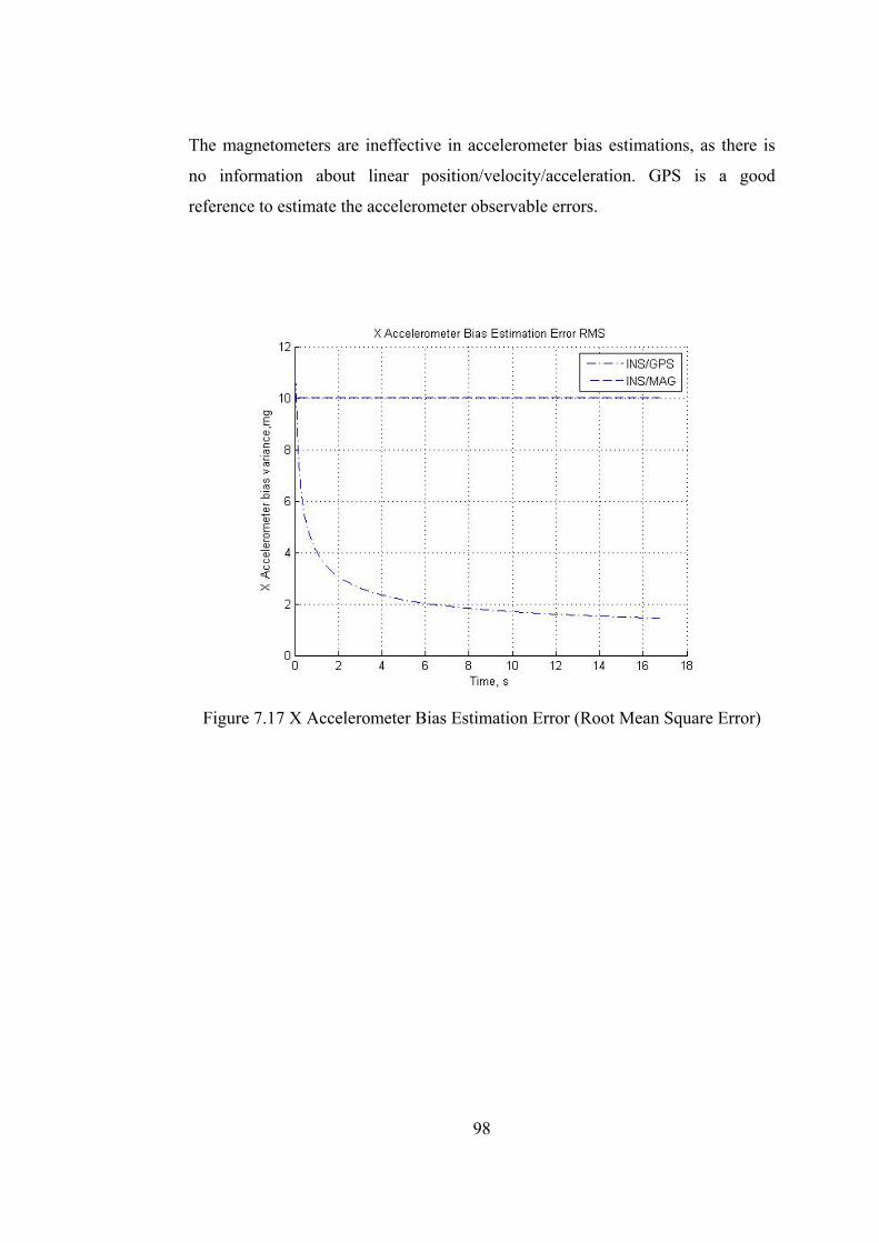
98
The magnetometers are ineffective in accelerometer bias estimations, as there is
no information about linear position/velocity/acceleration. GPS is a good
reference to estimate the accelerometer observable errors.
Figure 7.17 X Accelerometer Bias Estimation Error (Root Mean Square Error)
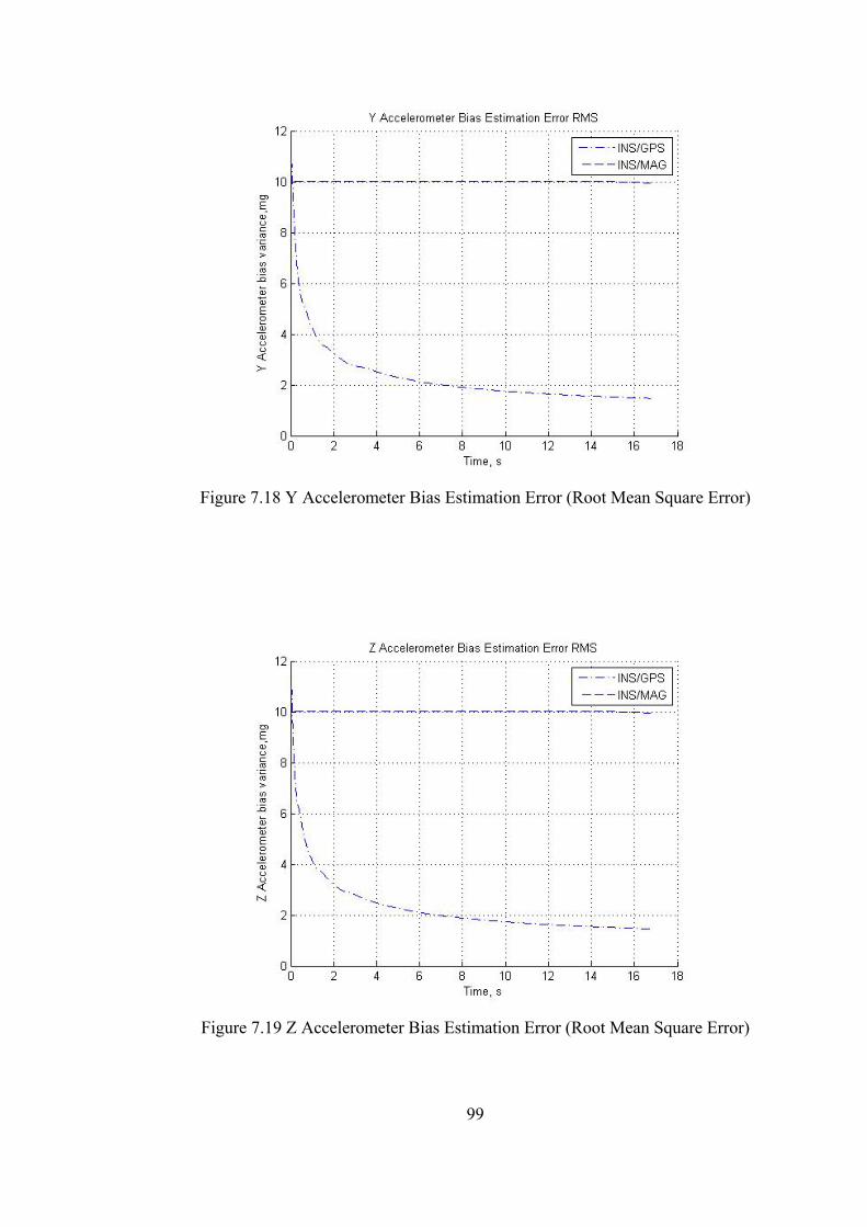
99
Figure 7.18 Y Accelerometer Bias Estimation Error (Root Mean Square Error)
Figure 7.19 Z Accelerometer Bias Estimation Error (Root Mean Square Error)
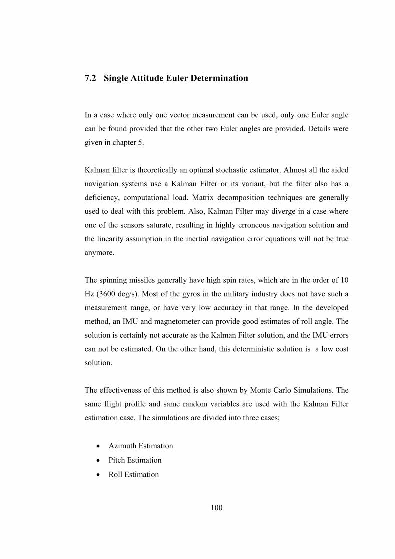
100
7.2 Single Attitude Euler Determination
In a case where only one vector measurement can be used, only one Euler angle
can be found provided that the other two Euler angles are provided. Details were
given in chapter 5.
Kalman filter is theoretically an optimal stochastic estimator. Almost all the aided
navigation systems use a Kalman Filter or its variant, but the filter also has a
deficiency, computational load. Matrix decomposition techniques are generally
used to deal with this problem. Also, Kalman Filter may diverge in a case where
one of the sensors saturate, resulting in highly erroneous navigation solution and
the linearity assumption in the inertial navigation error equations will not be true
anymore.
The spinning missiles generally have high spin rates, which are in the order of 10
Hz (3600 deg/s). Most of the gyros in the military industry does not have such a
measurement range, or have very low accuracy in that range. In the developed
method, an IMU and magnetometer can provide good estimates of roll angle. The
solution is certainly not accurate as the Kalman Filter solution, and the IMU errors
can not be estimated. On the other hand, this deterministic solution is a low cost
solution.
The effectiveness of this method is also shown by Monte Carlo Simulations. The
same flight profile and same random variables are used with the Kalman Filter
estimation case. The simulations are divided into three cases;
• Azimuth Estimation
• Pitch Estimation
• Roll Estimation
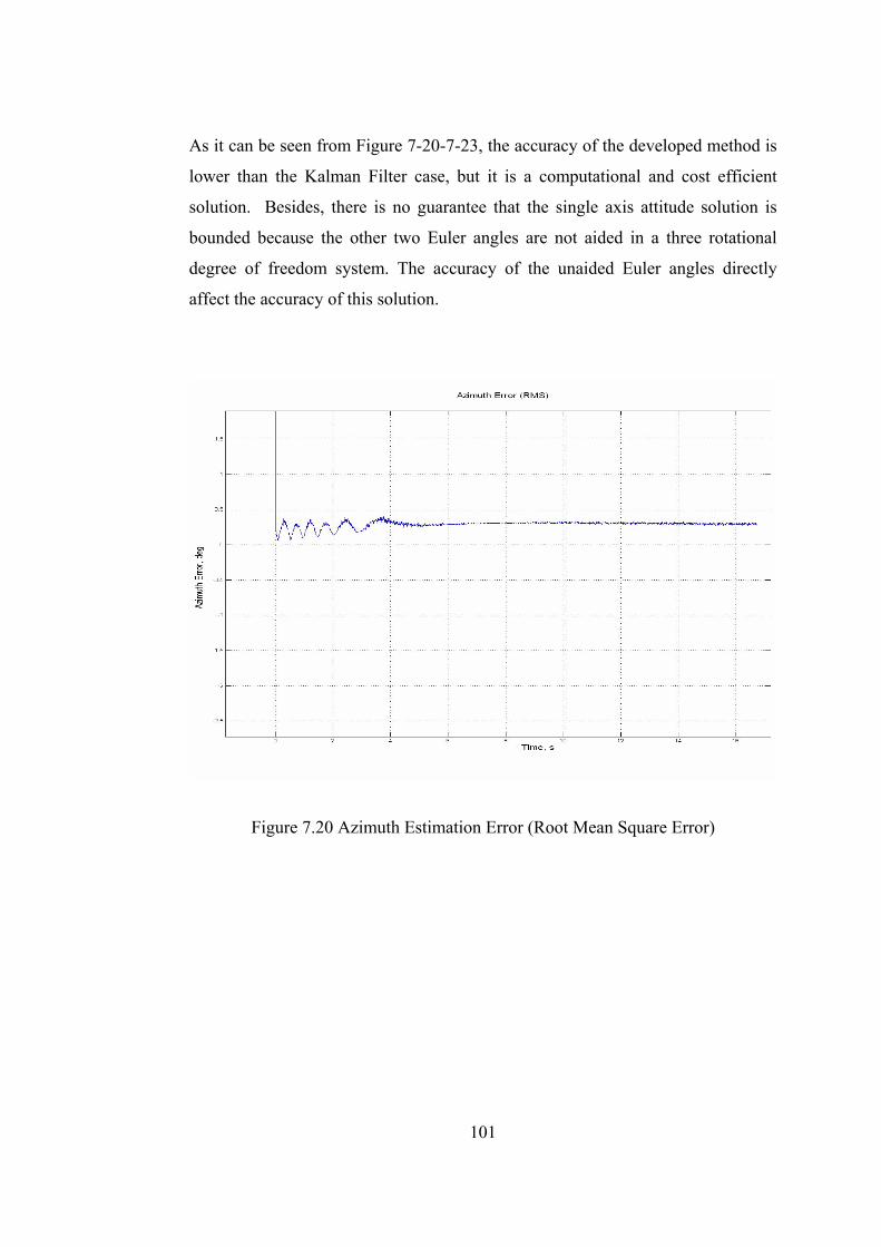
101
As it can be seen from Figure 7-20-7-23, the accuracy of the developed method is
lower than the Kalman Filter case, but it is a computational and cost efficient
solution. Besides, there is no guarantee that the single axis attitude solution is
bounded because the other two Euler angles are not aided in a three rotational
degree of freedom system. The accuracy of the unaided Euler angles directly
affect the accuracy of this solution.
Figure 7.20 Azimuth Estimation Error (Root Mean Square Error)
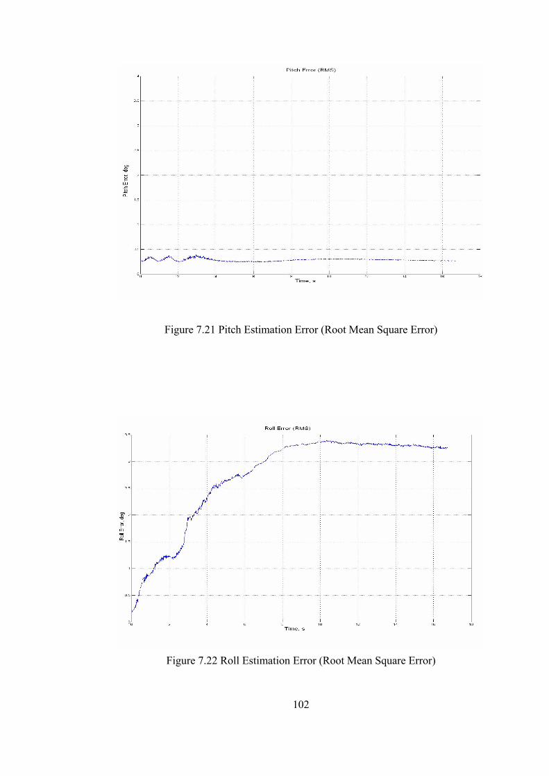
102
Figure 7.21 Pitch Estimation Error (Root Mean Square Error)
Figure 7.22 Roll Estimation Error (Root Mean Square Error)
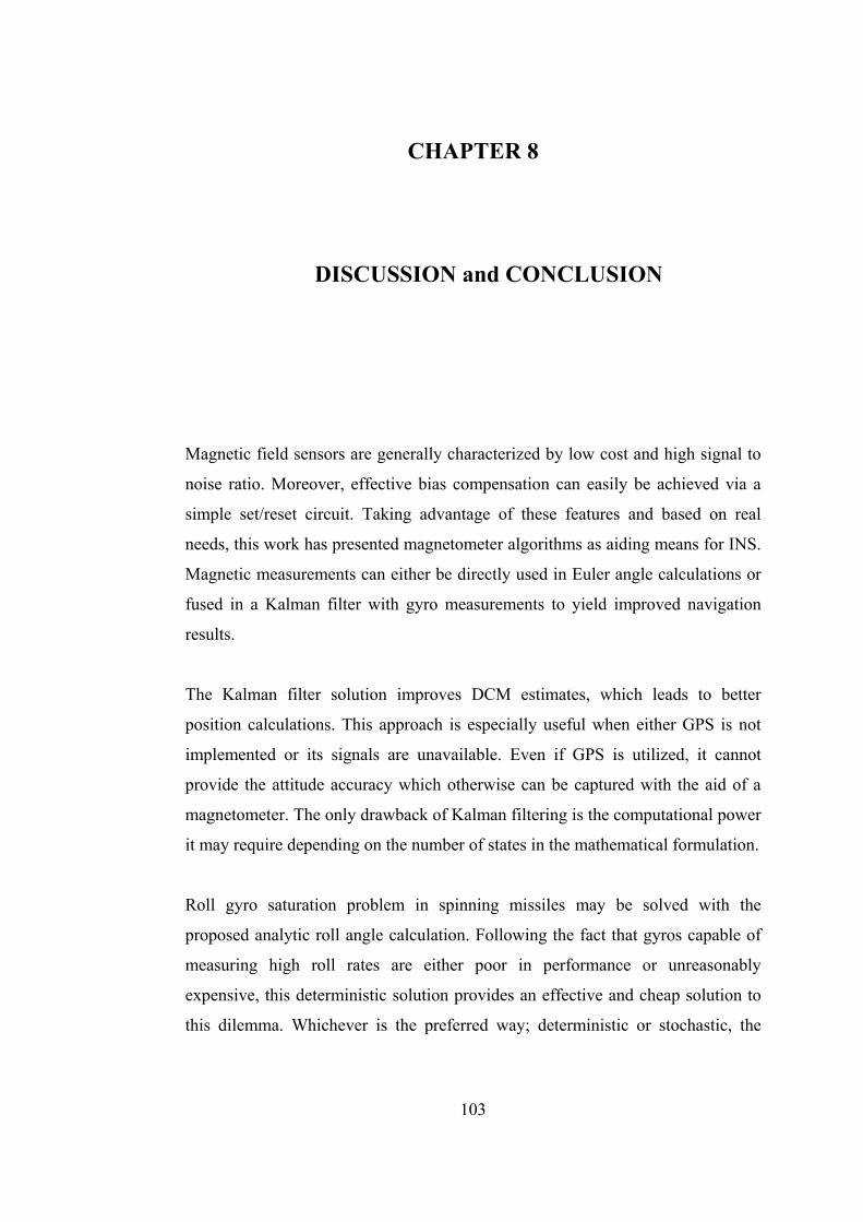
103
CHAPTER 8
8 DISCUSSION and CONCLUSION
Magnetic field sensors are generally characterized by low cost and high signal to
noise ratio. Moreover, effective bias compensation can easily be achieved via a
simple set/reset circuit. Taking advantage of these features and based on real
needs, this work has presented magnetometer algorithms as aiding means for INS.
Magnetic measurements can either be directly used in Euler angle calculations or
fused in a Kalman filter with gyro measurements to yield improved navigation
results.
The Kalman filter solution improves DCM estimates, which leads to better
position calculations. This approach is especially useful when either GPS is not
implemented or its signals are unavailable. Even if GPS is utilized, it cannot
provide the attitude accuracy which otherwise can be captured with the aid of a
magnetometer. The only drawback of Kalman filtering is the computational power
it may require depending on the number of states in the mathematical formulation.
Roll gyro saturation problem in spinning missiles may be solved with the
proposed analytic roll angle calculation. Following the fact that gyros capable of
measuring high roll rates are either poor in performance or unreasonably
expensive, this deterministic solution provides an effective and cheap solution to
this dilemma. Whichever is the preferred way; deterministic or stochastic, the
104
primary result of magnetometer algorithms is considerable reduction in gyro
costs.
In the modeling and simulation studies, following tasks are performed
1. Error model of a generic inertial measurement unit is derived
2. Linear error mechanization equations of a inertial navigation system is
derived with small attitude error assumptions
3. World Magnetic Field is embedded into simulation environment
4. Alternative magnetic field model is proposed.
5. Deterministic attitude determination equations with two vector sets are
derived.
6. Magnetometer measurement equations are derived for Kalman Filter
7. Single axis deterministic attitude determination algorithm is derived.
8. Experimental studies are carried for ground alignment
9. Monte Carlo simulations are done for ground alignment and in motion
estimations.
The developed navigation system has a self alignment capability, which is not the
case in unaided MEMS IMU. The classical two phase alignment process (coarse
and fine) is applied to the proposed system, resulting in a fast and accurate
alignment solution. Even in a RLG navigation unit, the ground alignment take at
least several minutes, where the magnetometer + IMU system aligns itself in a
few seconds.
The flight performance of the proposed system is demonstrated in a spinning
missile application. It is shown that magnetometer aiding is superior to GPS for
attitude and gyro error estimations. When the magnetometer + IMU system is
combined with GPS, not only the position and velocity errors become observable,
but also the accuracy and the convergence rate of the attitude and gyro error
estimations increases.
105
For a low computational cost solution, a single axis attitude determination
algorithm is developed. In the simulations, it is shown that the solution is not good
as Kalman Filter, but the computational load is very low relative to the stochastic
estimation filters.
This thesis has shown the effectiveness of magnetometer algorithms in navigation
calculations. However, the crucial issue that needs to be raised is about the
correctness of the measurements and reliability of the reference field model, and
the consistency between. Theoretically, these two are the representations of the
same vector in different frames. In practice; however, none of them will be
available without errors and/or uncertainties, which means that they will not be
equal when transformed from one frame to another. Consequently, care must be
taken in acquisition and interpretation of magnetic data. One imposed condition is
that in-vehicle magnetic disturbances must never affect sensor outputs. This can
be accomplished by convenient sensor placement and selection of non-magnetic
material. Secondly, the algorithms require that the outer field be known a priori as
a function of location. Over short ranges, this does not constitute a problem since
the directional and time derivatives of the Earth’s magnetic strength are
negligible; as a result, the reference magnetic vector can be approximated as
constant. Over long ranges; however, some other means of estimating the
reference vector becomes necessary. Mathematical models such as WMM2005
might be used here; but, one must be cautious against their applicability. There is
always possibility of being confronted by some outer, local magnetic disturbances
especially at low altitudes. These approximations are most accurate at sufficiently
high altitudes.
As a future work, real time in motion experiments can be done to demonstrate the
effectiveness of the developed algorithms. Thus, the effect of the magnetic
anomalies in the algorithms can be seen. Also, the alternative magnetic field
modeling can be applied to correct local WMM2005 errors.
106
REFERENCES
1. Titterton, D. H., Weston, J. L., Strapdown Inertial Navigation Technology, American Institute of Aeronautics and Astronautics & Institution of Electrical Engineers, 2004
2. Britting, Kenneth R. Inertial Navigation Systems Analysis. Wiley-Interscience, 1971.
3. Salychev, O.S., Applied Inertial Navigation: Problems and Solutions, BMSTU Press Moscow, Russia, 2004.
4. Psiaki, M. L., Martel, F., and Pal, P. K., “Three-Axis Attitude Determination via Kalman Filtering of Magnetometer Data,” Journal of Guidance, Control, and Dynamics, Vol. 13, No. 3, May-June 1990, pp. 506–514.
5. Lefferts, E. J., Markley, F. L., and Shuster, M. D., “Kalman Filtering for Spacecraft Attitude Estimation,” Journal of Guidance, Control, and Dynamics, Vol. 5, No. 5, Sept.-Oct. 1982, pp. 417–429.
6. Kok-Lam,.L., Crassidis, J.L.,Harman, R.R., “ Real Time Attitude Independent Gyro Calibration from 3 axis Magnetometer Measurements, AIAA-AAS Astrodynamics Specialist Conference and Exhibit, AIAA-2004-4855.
7. National Geomagnetic Information Center, website URL http://geomag.usgs.gov/.
8. Rogers, M.R., Applied Mathematics in Integrated Navigation Systems, AIAA, Inc., 2000.
9. Rogers R. M., Weapon IMU Transfer Alignment Using Aircraft Position from Actual Flight Tests, IEEE PLANS, pp328-335, 1996.
107
10. Yüksel,Y., “Design and Analysis of Transfer Alignment Algorithms”, METU Thesis,2005.
11. Savage, P., Strapdown Analytics: Part1-2, Strapdown Associates, Inc., Maple Plain, Minnesota, 2000.
12. Barbour N., Schmidt G. “Inertial sensor technology trends”, Proc. of 1998 Workshop on Autonomous Underwater Vehicles, August 1998, pp. 55-62.
13. Bose, S.C., GPS-INS Integrated Navigation Systems: Lecture Notes, Technalytics Inc., 2006.
14. Siouris, G.M., Aerospace Avionics Systems A Modern Synthesis, Academic Press Inc., 1993.
15. Scherzinger, B.M., “Inertial Navigator Error Models for Large Heading Uncertainty”, IEEE Position Location and Navigation Symposium, pp.477-484.
16. Chatfield, A.B. , Fundamentals of High Accuracy Inertial Navigation, Published by American Institute of Aeronautics and Astronautics, 1997.
17. Broxmeyer, C., Inertial Navigation Systems, McGraw-Hill Company Inc., USA, 1964.
18. Farrell, J.L., Integrated Aircraft Navigation, Academic Press Inc., London, England, 1976.
19. Bortz J.E., “A new mathematical formulation for strapdown inertial formulation”, IEEE Transactions on Aerospace and Electronic Systems, vol.7, no. 1, Jan. 1971, pp. 61-66.
20. Savage P. G., “Strapdown System Algorithms, Advances in Strapdown
Inertial Systems”, NATO AGARD Lecture Series, No:133, 1984.
21. Ignagni M.B., “Optimal strapdown attitude integration algorithms”, Journal of Guidance, Control, and Dynamics, vol. 13, no. 2, March-April 1990, pp.363-369.
22. Savage P. G., Strapdown System Performance Analysis, Advances in Navigation and Integration Technology , NATO RTO Sensors and Electronics Technology Lecture Series, No:64, 2003.
108
23. Bar-Itzhack, Berman N., “Control Theoretic Approach to Inertial
Navigation Systems”, Journal of Guidance and Control, Vol.11, No. 3, 1988.
24. Caruso, M.J., “A New Perspective On Magnetic Field Sensing”, Sensor Magazine Online, December 1998.
25. Caruso, M.J., “Application of Magnetic Sensors for Low Cost Compass Systems”, Honeywell A.N., 2004.
26. Brown G.B., Hwang P.Y.C., Introduction to Random Signals and Applied Kalman Filtering, 1992, John Wiley & Sons Inc.
27. Gelb A., Applied Optimal Estimation, 1974, MIT Press.
28. Shin, E. “Estimation Techniques for Low-Cost Inertial Navigation”, PhD. Thesis, University of Calgary, Department of Geomatics Engineering, May 2005.
29. Biezad, J.D., Satellite Navigation Systems Lecture Notes, Calpoly , 2004.
30. Maybeck, P.S., Stochastic Models, Estimation, and Control, Volume 1-2, Academic Press Inc., 1979.
31. Wahba, G., and et. al. Problem 65-1 (Solution). SIAM, Review, 8:384-386, 1966.
32. Schimelevich, L., Naor, R., “New Approach to Coarse Alignment”, IEEE Position Location and Navigation Symposium, 1996, pp. 324-327.
33. A Gyro free Quaternion Based Attitude Determination System Suitable for Implementation Using Low Cost Sensor”, IEEE 2000 Position Location and Navigation Symposium, pp185-192, 2000.
34. Fleck,V., Sommer,E., Brökelmann,M., Study of Real-time Filtering for an Inertial Measurement Unit(IMU) with Magnetometer in a 155mm Projectile“,IEEE 2006 Position Location and Navigation Symposium, pp803-807, 1998.
109
35. Aspects of pure and satellite aided Inertial Navigation for Gun Launched Munitions IEEE 2004 Position Location and Navigation Symposium, pp327-336, 2004.
36. Fang, J.C., Wan, D.J., “A Fast Initial Alignment Method for Strapdown Inertial Navigation System on Stationary Base”, IEEE Transactions on Aerospace and Electronic Systems, Vol. 32, No. 4, 1996, pp. 1501-1505.
37. Park, H.W. , Lee, J.G. , Park, C.G. , “Error Analysis of Strapdown Inertial Navigation System Aligned by Gyrocompassing,” Proceedings of the 1995 IFAC Intelligent Automation Control in Aerospace, Beijing, China, August 1995, pp. 191-195.
38. Eduardo, N. Hugh, D.W., “Initial Calibration and Alignment of an Inertial Navigation,” IEEE Position Location and Navigation Symposium, 1997, pp. 175-180.
39. Klotz H. A., Derbak C. B., GPS-Aided Navigation and Unaided Navigation on the Joint Direct Attack Munition, IEEE 1998 Position Location and Navigation Symposium, pp412-419, 1998.
40. Gorecki, R.M., A Baseline 6 Degree of Freedom Generic Missile Simulation, Defense System and Technology, DSTO-TR-0931, 2003.
41. Seymen ,N.B., “Robust Set Valued Estimation and It’s Application to In-
Flight Alignment of SINS”, METU Thesis,2005.

110
APPENDIX A
A WORLD MAGNETIC MODEL 2005
A.1 World Magnetic Model
The Earth’s magnetic field (B) is a vector quantity varying in space (r) and time
(t). The field, as measured by a magnetic sensor on or above the Earth’s surface, is
actually a composite of several magnetic fields, generated by a variety of sources.
These fields are superimposed on each other and through inductive processes
interact with each other. The most important of these geomagnetic sources are:
1. The main field (Figure 1), generated in Earth’s conducting, fluid outer
core (Bm);
2. The crustal field from Earth’s crust/upper mantle (Bc);
3. The combined disturbance field from electrical currents flowing in the
upper atmosphere and magnetosphere, which also induce electrical
currents in the sea and the ground (Bd)
Thus, the observed magnetic field is a sum of these contributions
( , ) ( , ) ( , ) ( , )m c dB r t B r t B r t B r t= + + (A.1)
111
Bm is the dominating part of the field, accounting for over 95% of the field
strength at the Earth’s surface. Secular variation is the slow change in time of
Bm. Bc, the field arising from magnetized crustal rocks, varies spatially, but is
considered constant in time for the time-scales considered here. Bc is usually
much smaller in magnitude than Bm. The crustal field is constant over the time-
scales considered here. The field arising from currents flowing in the ionosphere
and magnetosphere and their resultant induced currents in the Earth’s mantle and
crust, Bd, varies both with location and time. The WMM represents only the main
geomagnetic field, Bm. To create an accurate main field model, it is necessary to
have data with good global coverage and as low a noise level as possible. The
Danish Ørsted and German CHAMP satellite data sets satisfy these requirements.
Both satellites provide high quality vector and scalar data at all latitudes and
longitudes, but not during all time periods needed for modeling. These satellite
data were therefore augmented with ground observatory hourly mean data, which
were available almost continuously over the period of interest, although with
poorer spatial coverage. The observatory data therefore provide valuable
constraints on the time variations of the geomagnetic field. Used together, satellite
and observatory data provide an exceptional quality data set for modeling the
behavior of the main magnetic field in space and time. Bc has spatial variations on
the order of meters to thousands of kilometers and cannot be fully modeled with
low degree spherical harmonic models. Therefore, the WMM does not include
contributions from the crust except for those of very long wavelength. Bc is
usually smaller at sea than on land, and decreases with increasing altitude. The
rock magnetization resulting in Bc may be either induced (by the main magnetic
field) or remnant or a combination of both. The field arising from currents flowing
in the ionosphere and magnetosphere and their associated induced currents in the
Earth, Bd, varies both with location and time. The regular variations are both
diurnal and annual and they are essentially generated by the daylit atmosphere at
altitudes of 100-130 km, ionized by the Sun’s radiation, being moved in the
Earth’s main field by winds and tides, thus producing the necessary conditions
(motion of a conductor in a magnetic field) for a dynamo to operate. Further daily
112
and annual variations are caused by the rotation of the Earth in the external
magnetosphere field, which is organized in a sun-synchronous reference frame.
The irregular variations are due to magnetic storms and sub storms. Magnetic
storms generally have three phases: an initial phase, often with a sudden
commencement and increased horizontal field at mid-latitudes, a main phase, and
a recovery phase. The main phase involves an intensification of the ring current
from the plasma sheet.
During the recovery phase the ring current returns to normal over a number of
days and associated sub-storms subside. Magnetic storm and sub-storm effects are
generally more severe at high geomagnetic latitudes where the ionized region of
the upper atmosphere (the ionosphere) is coupled to the magnetosphere by field-
aligned currents and is therefore strongly influenced by the interplanetary
magnetic field and current systems in the magneto tail. Both the regular and
irregular disturbance field variations are modulated by season and the solar
magnetic activity cycle. The primary disturbance field is often known as the
external field, as its main sources, the ionosphere and magnetosphere, are external
to the surface of the Earth where geomagnetic measurements were traditionally
made. However, this term can be confusing and is avoided when using satellite
data, as the ionosphere is below the altitude of these data and is therefore
effectively internal to this observation surface.
A.2 Model Parameterization
The geomagnetic field measured at the Earth’s surface or at satellite altitude is the
sum of the fields generated by sources internal or external to the solid Earth.
Away from its sources, the internal magnetic field B is a potential field and
therefore can be written as the negative gradient of a scalar potential
( , , , ) ( , , , )B r t V r tϕ λ ϕ λ′ ′= −∇ (A.1)
113
This potential can be expanded in terms of spherical harmonics:
1
1 1
( , , , )
( ( )cos( ) ( )sin( ))( ) (sin )N N
m m n mn n n
n m
V r taa g t m h t m Pr
ϕ λ
λ λ ϕ+
= =
′ =
⎧ ⎫′+⎨ ⎬⎩ ⎭∑∑
(A.2)
where a (6371.2 km) is the standard Earth’s magnetic reference radius ( , , )rϕ λ′ are
the latitude, longitude and radius in a spherical, geocentric reference frame,
( ( ), ( ))m mn ng t h t are the time-dependent Gauss coefficients of degree n and order m
describing internal sources. (sin )mnP ϕ′ are the Schmidt semi-normalized
Associated Legendre Functions, defined as
( )!(sin ) 2 (sin )( )!
m mn n
n mP Pn m
ϕ ϕ−′ ′=+
if m > 0
(sin ) (sin )m mn nP Pϕ ϕ′ ′= if m=0 (A.3)
WMM 2005 used 36 = N as the truncation level of the internal expansion. The
internal Gauss coefficients from degree 1 to 8 are assumed to have a quadratic
dependence on time,
20 0
20 0
1( ) ( ) ( )2
1( ) ( ) ( )2
m m m mn n n n
m m m mn n n n
g t g g t t g t t
h t h h t t h t t
= + − + −
= + − + − (A.4)
where, on the left side, ( )mng t and ( )m
nh t are time varying functions,
while , , , , ,m m m m m mn n n n n ng g g h h h denote constants. The time is given in decimal year
and 0 t is the reference date of the model, chosen to be at the approximate mid-
point of the time span of satellite and observatory hourly mean values (2002.0).
From degree 9 up to 12 a linear dependence on time of the internal Gauss
114
coefficients is assumed, and, for higher degrees, the internal Gauss coefficients
are assumed to be constant with time. These truncation levels are chosen as the
degrees up to which coefficients can be determined robustly without recourse to
damping.
This model given by WMM 2005 is valid only for sources internal to the Earth,
like the main field and the crustal field. For the external field, caused by currents
in the ionosphere and magnetosphere, a spherical harmonic representation can be
used. However, the external fields are organized in a sun synchronous reference
frame. WMM 2005 parent model includes a constant degree-2 parameterization of
magnetospheric fields in a sunsynchronous reference frame. For an earth-fixed,
rotating observer, these external fields are perceived to have daily and seasonal
variations. Our parent model accounts for these periodic variations, as well as for
their electromagnetic induction in the Earth.
Following evidence of a penetration of the Interplanetary Magnetic Field (IMF),
an IMF By correlated component in a sun-synchronous reference frame was
included in the modeling. This component reaches about half of the IMF By at the
Earth’s surface, with typical strengths of 1-2 nT.
Tidal movement of conducting seawater through the Earth’s magnetic field
induces electric fields, currents, and secondary magnetic fields, which reach about
7 nT at the ocean surface and 3 nT at satellite altitude. These fields are clearly
visible in satellite data and closely coincide with independent predictions from
tidal ocean flow models. The satellite measurements were corrected for the eight
major tidal constituents.
Finally, when the data set contains hourly mean observatory data, offsets at each
observatory have to be introduced to take into account the local field, mainly
generated in the crust, which cannot be described by the model. Then, at an
observatory, the magnetic field B is:
( , , , ) ( , , , ) ( , , )B r t V r t O rϕ λ ϕ λ ϕ λ′ ′ ′= −∇ + (A.5)
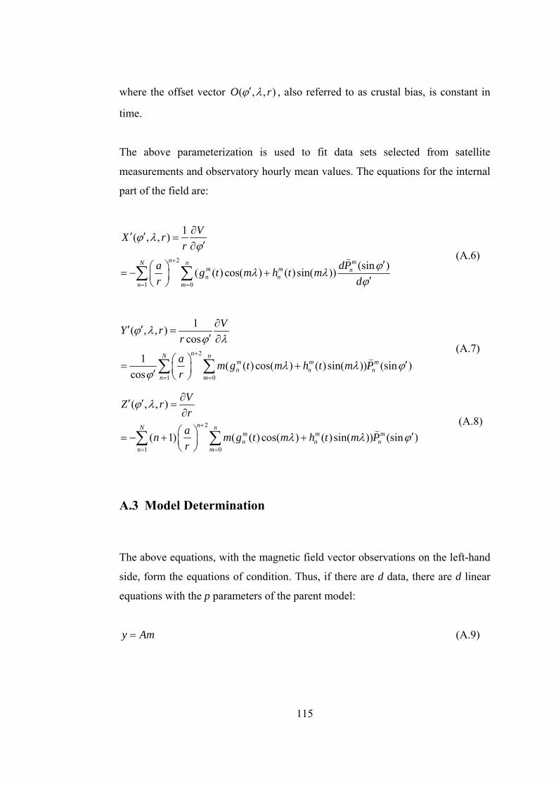
115
where the offset vector ( , , )O rϕ λ′ , also referred to as crustal bias, is constant in
time.
The above parameterization is used to fit data sets selected from satellite
measurements and observatory hourly mean values. The equations for the internal
part of the field are:
2
1 0
1( , , )
(sin )( ( ) cos( ) ( )sin( ))n mN n
m m nn n
n m
VX rr
dPa g t m h t mr d
ϕ λϕ
ϕλ λϕ
+
= =
∂′ ′ =′∂
′⎛ ⎞= − +⎜ ⎟ ′⎝ ⎠∑ ∑
(A.6)
2
1 0
1( , , )cos
1 ( ( ) cos( ) ( )sin( )) (sin )cos
nN nm m mn n n
n m
VY rr
a m g t m h t m Pr
ϕ λϕ λ
λ λ ϕϕ
+
= =
∂′ ′ =′ ∂
⎛ ⎞ ′= +⎜ ⎟′ ⎝ ⎠∑ ∑
(A.7)
2
1 0
( , , )
( 1) ( ( ) cos( ) ( )sin( )) (sin )nN n
m m mn n n
n m
VZ rr
an m g t m h t m Pr
ϕ λ
λ λ ϕ+
= =
∂′ ′ =∂
⎛ ⎞ ′= − + +⎜ ⎟⎝ ⎠
∑ ∑ (A.8)
A.3 Model Determination
The above equations, with the magnetic field vector observations on the left-hand
side, form the equations of condition. Thus, if there are d data, there are d linear
equations with the p parameters of the parent model:
y Am= (A.9)
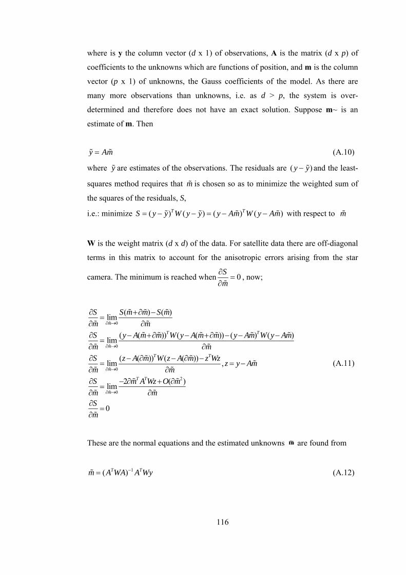
116
where is y the column vector (d x 1) of observations, A is the matrix (d x p) of
coefficients to the unknowns which are functions of position, and m is the column
vector (p x 1) of unknowns, the Gauss coefficients of the model. As there are
many more observations than unknowns, i.e. as d > p, the system is over-
determined and therefore does not have an exact solution. Suppose m~ is an
estimate of m. Then
y Am= (A.10)
where y are estimates of the observations. The residuals are ( )y y− and the least-
squares method requires that m is chosen so as to minimize the weighted sum of
the squares of the residuals, S,
i.e.: minimize ( ) ( ) ( ) ( )T TS y y W y y y Am W y Am= − − = − − with respect to m
W is the weight matrix (d x d) of the data. For satellite data there are off-diagonal
terms in this matrix to account for the anisotropic errors arising from the star
camera. The minimum is reached when 0Sm
∂=
∂, now;
0
0
0
2
0
( ) ( )lim
( ( )) ( ( )) ( ) ( )lim
( ( )) ( ( ))lim ,
2 ( )lim
0
m
T T
m
T T
m
T T
m
S S m m S mm mS y A m m W y A m m y Am W y Amm mS z A m W z A m z Wz z y Amm mS m A Wz O mm mSm
∂ →
∂ →
∂ →
∂ →
∂ +∂ −=
∂ ∂∂ − +∂ − +∂ − − −
=∂ ∂∂ − ∂ − ∂ −
= = −∂ ∂∂ − ∂ + ∂
=∂ ∂∂
=∂
(A.11)
These are the normal equations and the estimated unknowns are found from
1( )T Tm A WA A Wy−= (A.12)
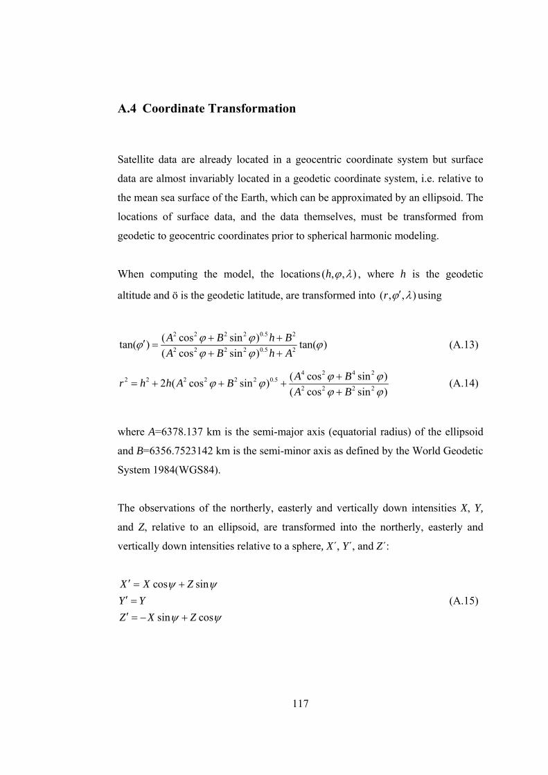
117
A.4 Coordinate Transformation
Satellite data are already located in a geocentric coordinate system but surface
data are almost invariably located in a geodetic coordinate system, i.e. relative to
the mean sea surface of the Earth, which can be approximated by an ellipsoid. The
locations of surface data, and the data themselves, must be transformed from
geodetic to geocentric coordinates prior to spherical harmonic modeling.
When computing the model, the locations ( , , )h ϕ λ , where h is the geodetic
altitude and ö is the geodetic latitude, are transformed into ( , , )r ϕ λ′ using
2 2 2 2 0.5 2
2 2 2 2 0.5 2
( cos sin )tan( ) tan( )( cos sin )A B h BA B h A
ϕ ϕϕ ϕϕ ϕ
+ +′ =+ +
(A.13)
4 2 4 22 2 2 2 2 2 0.5
2 2 2 2
( cos sin )2 ( cos sin )( cos sin )A Br h h A BA B
ϕ ϕϕ ϕϕ ϕ
+= + + +
+ (A.14)
where A=6378.137 km is the semi-major axis (equatorial radius) of the ellipsoid
and B=6356.7523142 km is the semi-minor axis as defined by the World Geodetic
System 1984(WGS84).
The observations of the northerly, easterly and vertically down intensities X, Y,
and Z, relative to an ellipsoid, are transformed into the northerly, easterly and
vertically down intensities relative to a sphere, X´, Y´, and Z´:
cos sin
sin cos
X X ZY YZ X Z
ψ ψ
ψ ψ
′ = +′ =′ = − +
(A.15)
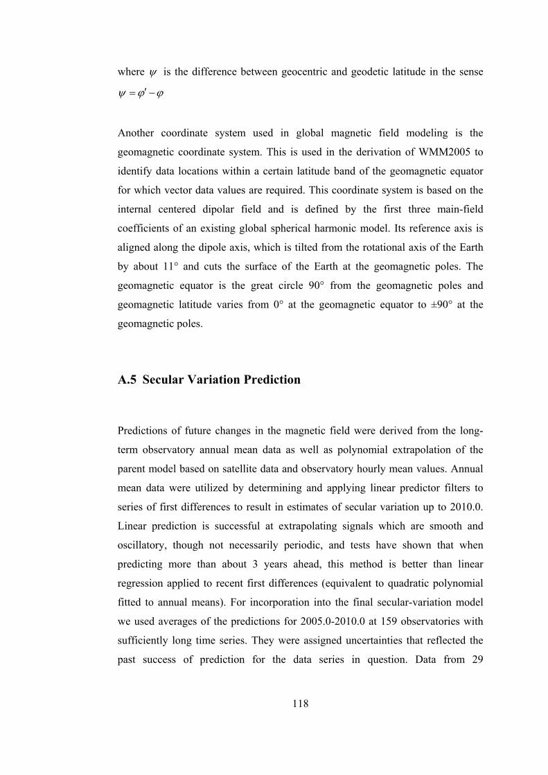
118
where ψ is the difference between geocentric and geodetic latitude in the sense
ψ ϕ ϕ′= −
Another coordinate system used in global magnetic field modeling is the
geomagnetic coordinate system. This is used in the derivation of WMM2005 to
identify data locations within a certain latitude band of the geomagnetic equator
for which vector data values are required. This coordinate system is based on the
internal centered dipolar field and is defined by the first three main-field
coefficients of an existing global spherical harmonic model. Its reference axis is
aligned along the dipole axis, which is tilted from the rotational axis of the Earth
by about 11° and cuts the surface of the Earth at the geomagnetic poles. The
geomagnetic equator is the great circle 90° from the geomagnetic poles and
geomagnetic latitude varies from 0° at the geomagnetic equator to ±90° at the
geomagnetic poles.
A.5 Secular Variation Prediction
Predictions of future changes in the magnetic field were derived from the long-
term observatory annual mean data as well as polynomial extrapolation of the
parent model based on satellite data and observatory hourly mean values. Annual
mean data were utilized by determining and applying linear predictor filters to
series of first differences to result in estimates of secular variation up to 2010.0.
Linear prediction is successful at extrapolating signals which are smooth and
oscillatory, though not necessarily periodic, and tests have shown that when
predicting more than about 3 years ahead, this method is better than linear
regression applied to recent first differences (equivalent to quadratic polynomial
fitted to annual means). For incorporation into the final secular-variation model
we used averages of the predictions for 2005.0-2010.0 at 159 observatories with
sufficiently long time series. They were assigned uncertainties that reflected the
past success of prediction for the data series in question. Data from 29
119
observatories, which had time series too short for the application of linear
prediction filters, were also used by computing average secular-variation
estimates and assuming that these did not change with time.
A.6 Derivation of World Magnetic Model
The final main-field coefficients for 2005.0 were derived by polynomial
extrapolation of the main-field Gauss coefficients from the parent model to this
date.
Before the final secular-variation coefficients could be derived, the secular-
variation estimates from the parent model (valid for 1999.0-2004.5) were
combined with the long-term predictions at the observatories described in Section
4.4. This was done by using the parent model to estimate annual rates of change in
the north, east and vertically down directions, in a geocentric coordinate system,
at the centers of 1654 equal-area tessera. Each tessera was equivalent in size to a
5° latitude by 5° longitude box at the equator. This synthetic dataset was
combined with the predicted mean X, Y and Z rates of change for 2005.0-2010.0 at
the 188 observatories, rotated into a geocentric coordinate system. Equations (8)-
(10) of Section 4.1, with the time varying Gauss coefficients ( )mng t , ( )m
nh t
replaced by their derivatives mng and m
nh were then used to determine the final
secular-variation coefficients.
A.7 Resulting Model
This section lists the final model coefficients, the corresponding magnetic pole
and eccentric dipole locations, provides the equations for computing the magnetic
field components at a given location, and discusses the accuracy and limitations of
the model.

120
A.8 Model Coefficients
The model coefficients also referred to as Gauss coefficients; provide an accurate
and convenient representation of the Earth’s main magnetic field. Their values are
listed in Table A.1. These coefficients can be used to compute values for the field
elements and their annual rates of change at any location near the surface of the
Earth and at any date between 2005.0 and 2010.0.
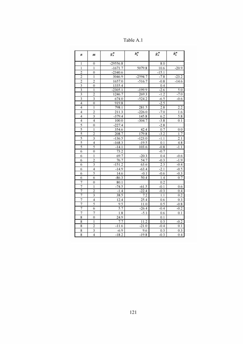
121
Table A.1

122
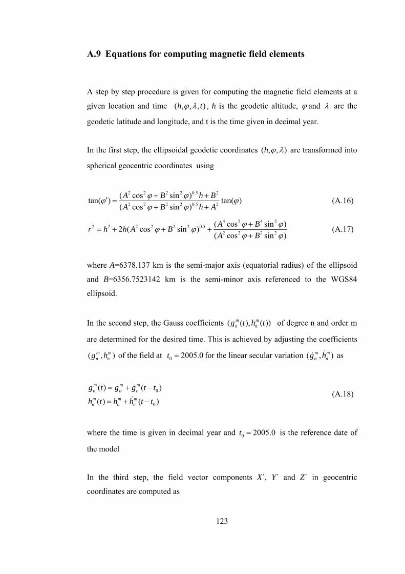
123
A.9 Equations for computing magnetic field elements
A step by step procedure is given for computing the magnetic field elements at a
given location and time ( , , , )h tϕ λ , h is the geodetic altitude, ϕ and λ are the
geodetic latitude and longitude, and t is the time given in decimal year.
In the first step, the ellipsoidal geodetic coordinates ( , , )h ϕ λ are transformed into
spherical geocentric coordinates using
2 2 2 2 0.5 2
2 2 2 2 0.5 2
( cos sin )tan( ) tan( )( cos sin )A B h BA B h A
ϕ ϕϕ ϕϕ ϕ
+ +′ =+ +
(A.16)
4 2 4 22 2 2 2 2 2 0.5
2 2 2 2
( cos sin )2 ( cos sin )( cos sin )A Br h h A BA B
ϕ ϕϕ ϕϕ ϕ
+= + + +
+ (A.17)
where A=6378.137 km is the semi-major axis (equatorial radius) of the ellipsoid
and B=6356.7523142 km is the semi-minor axis referenced to the WGS84
ellipsoid.
In the second step, the Gauss coefficients ( ( ), ( ))m mn ng t h t of degree n and order m
are determined for the desired time. This is achieved by adjusting the coefficients
( , )m mn ng h of the field at 0 2005.0t = for the linear secular variation ( , )m m
n ng h as
0
0
( ) ( )
( ) ( )
m m mn n n
m m mn n n
g t g g t t
h t h h t t
= + −
= + − (A.18)
where the time is given in decimal year and 0 2005.0t = is the reference date of
the model
In the third step, the field vector components X´, Y´ and Z´ in geocentric
coordinates are computed as
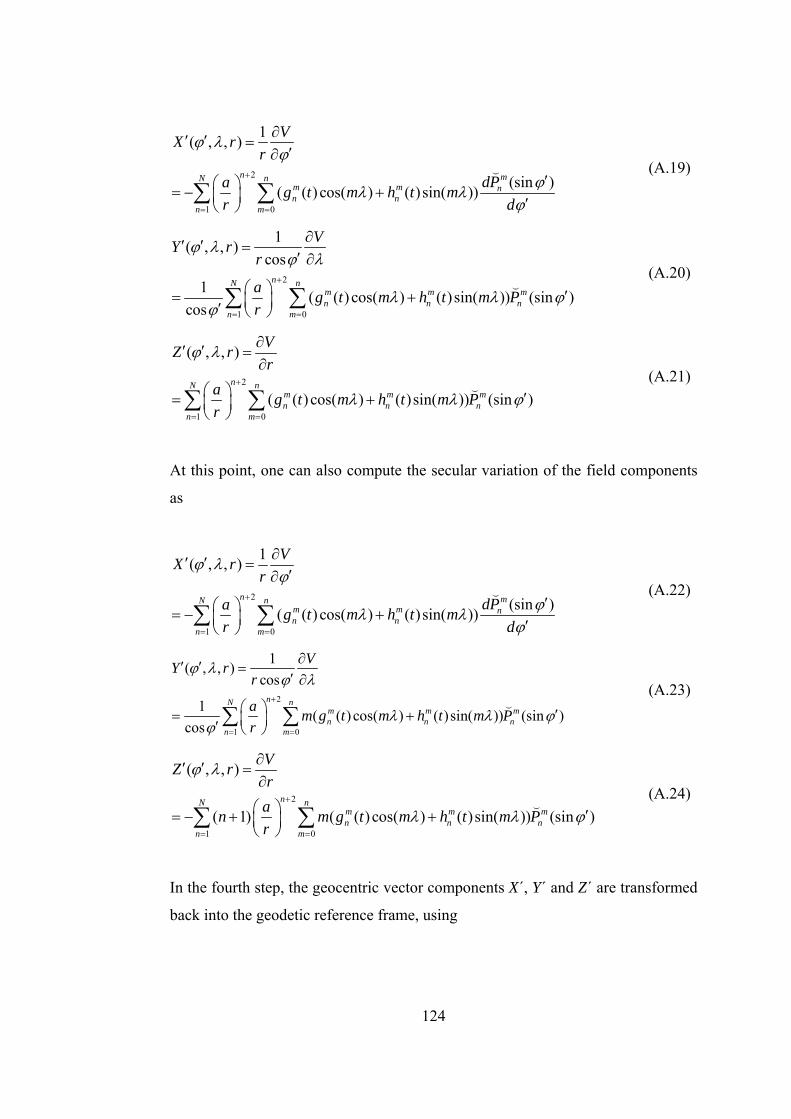
124
2
1 0
1( , , )
(sin )( ( ) cos( ) ( )sin( ))n mN n
m m nn n
n m
VX rr
dPa g t m h t mr d
ϕ λϕ
ϕλ λϕ
+
= =
∂′ ′ =′∂
′⎛ ⎞= − +⎜ ⎟ ′⎝ ⎠∑ ∑
(A.19)
2
1 0
1( , , )cos
1 ( ( ) cos( ) ( )sin( )) (sin )cos
nN nm m mn n n
n m
VY rr
a g t m h t m Pr
ϕ λϕ λ
λ λ ϕϕ
+
= =
∂′ ′ =′ ∂
⎛ ⎞ ′= +⎜ ⎟′ ⎝ ⎠∑ ∑
(A.20)
2
1 0
( , , )
( ( ) cos( ) ( )sin( )) (sin )nN n
m m mn n n
n m
VZ rr
a g t m h t m Pr
ϕ λ
λ λ ϕ+
= =
∂′ ′ =∂
⎛ ⎞ ′= +⎜ ⎟⎝ ⎠
∑ ∑ (A.21)
At this point, one can also compute the secular variation of the field components
as
2
1 0
1( , , )
(sin )( ( ) cos( ) ( )sin( ))n mN n
m m nn n
n m
VX rr
dPa g t m h t mr d
ϕ λϕ
ϕλ λϕ
+
= =
∂′ ′ =′∂
′⎛ ⎞= − +⎜ ⎟ ′⎝ ⎠∑ ∑
(A.22)
2
1 0
1( , , )cos
1 ( ( ) cos( ) ( )sin( )) (sin )cos
nN nm m mn n n
n m
VY rr
a m g t m h t m Pr
ϕ λϕ λ
λ λ ϕϕ
+
= =
∂′ ′ =′ ∂
⎛ ⎞ ′= +⎜ ⎟′ ⎝ ⎠∑ ∑
(A.23)
2
1 0
( , , )
( 1) ( ( ) cos( ) ( )sin( )) (sin )nN n
m m mn n n
n m
VZ rr
an m g t m h t m Pr
ϕ λ
λ λ ϕ+
= =
∂′ ′ =∂
⎛ ⎞ ′= − + +⎜ ⎟⎝ ⎠
∑ ∑ (A.24)
In the fourth step, the geocentric vector components X´, Y´ and Z´ are transformed
back into the geodetic reference frame, using
125
cos sin
sin cos
X X ZY YZ X Z
ψ ψ
ψ ψ
′ ′= +′=
′ ′= − + (A.25)
where ψ ϕ ϕ′= − is the difference between geocentric and geodetic latitude and
′ϕ was computed in step 1. Similarly, the time derivatives of the vector
components are transformed using
cos sin
sin cos
X X ZY YZ X Z
ψ ψ
ψ ψ
′ ′= +
′=
′ ′= − +
(A.26)
In the last step, the magnetic elements H, F, D, I, and the grid variation, GV, are
computed from the vector components as
2 2 2 2, , arctan( , ), arctan( , )
, 55, 55
o
o
H X Y F H Z D Y X I Z HGV D forGV D for
λ ϕ
λ ϕ
= + = + = =
= − >
= + < −
(A.27)
For H=0 the declination is undefined.
The secular variation of these elements is computed using
2
2
. .
. . .
180 . .
180 . .
X X Y YHH
X X Y Y Z ZFF
X Y Y XDH
H Z Z HIF
GV D
π
π
+=
+ +=
−=
−=
=
(A.28)
126
where D , I and GV are given in degrees/year. Here, the factor 180π
converts from
radians to degree. This conversion factor is not present in equation (A.29),
assuming that the arctan function provides the result in degrees.
A.10 Model Limitations
It is important to recognize that the WMM geomagnetic model and the charts
produced from this model characterize only that portion of the Earth’s magnetic
field that is generated by dynamo action in the Earth’s fluid outer core (Bm). The
portions of the geomagnetic field generated by the Earth’s crust and upper mantle
(Bc), and by the ionosphere and magnetosphere (Bd), are not represented in the
WMM. Consequently, a magnetic sensor such as a compass or magnetometer may
observe spatial and temporal magnetic anomalies when referenced to the WMM.
In particular, certain local, regional, and temporal magnetic declination anomalies
can exceed 10 degrees. Anomalies of this magnitude are not common but they do
exist. Declination anomalies of the order of 3 or 4 degrees are not uncommon but
are of small spatial extent and are relatively isolated. On land, spatial anomalies
are produced by mountain ranges, ore deposits, ground struck by lightning,
geological faults, and cultural features such as trains, planes, tanks, railroad
tracks, power lines, etc. The corresponding deviations are usually smaller at sea,
and decrease with increasing altitude of an aircraft or spacecraft. In ocean areas,
these anomalies occur most frequently along continental margins, near seamounts,
and near ocean ridges, trenches, and fault zones, particularly those of volcanic
origin. Ships and submarines are also sources of magnetic anomalies in the ocean.
The crustal contributions could be included in an extended model, expanded to
high degrees, as is common for modern gravity field models. Since the crustal
field is almost constant in time, it can be inferred from all available marine,
aeromagnetic, and high resolution CHAMP and future SWARM satellite data,
measured at all times. However, this extended model would differ significantly in
format from the current WMM, requiring changes in supporting software.
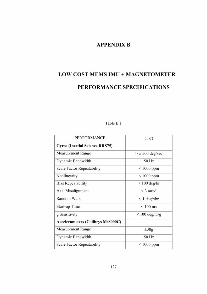
127
APPENDIX B
B LOW COST MEMS IMU + MAGNETOMETER
PERFORMANCE SPECIFICATIONS
Table B.1
PERFORMANCE (1 σ)
Gyros (Inertial Science RRS75)
Measurement Range > ± 500 deg/sec
Dynamic Bandwidth 50 Hz
Scale Factor Repeatability < 1000 ppm
Nonlinearity < 1000 ppm
Bias Repeatability < 100 deg/hr
Axis Misalignment ≤ 3 mrad
Random Walk ≤ 1 deg/√hr
Start-up Time ≤ 100 ms
g Sensitivity < 100 deg/hr/g
Accelerometers (Colibrys Ms8000C)
Measurement Range ±30g
Dynamic Bandwidth 50 Hz
Scale Factor Repeatability < 1000 ppm
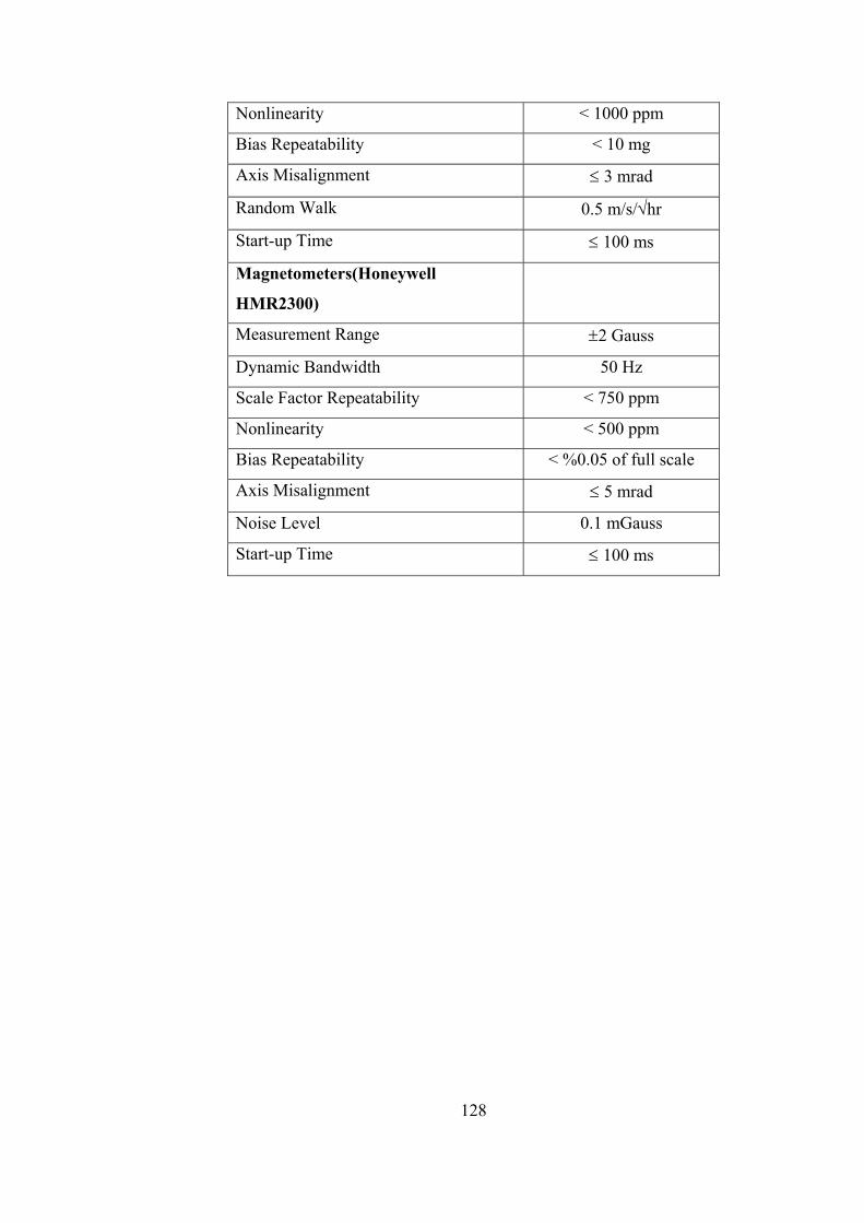
128
Nonlinearity < 1000 ppm
Bias Repeatability < 10 mg
Axis Misalignment ≤ 3 mrad
Random Walk 0.5 m/s/√hr
Start-up Time ≤ 100 ms
Magnetometers(Honeywell
HMR2300)
Measurement Range ±2 Gauss
Dynamic Bandwidth 50 Hz
Scale Factor Repeatability < 750 ppm
Nonlinearity < 500 ppm
Bias Repeatability < %0.05 of full scale
Axis Misalignment ≤ 5 mrad
Noise Level 0.1 mGauss
Start-up Time ≤ 100 ms
129
APPENDIX C
C DERIVATION OF INERTIAL NAVIGATION
MECHANIZATION EQUATIONS
In this system, it is required to calculate the vehicle speed with respect to earth,
the ground speed, in inertial axes, denoted by iev . First of all, it is essential to
express the fundamental navigation equations[17,18]
2
2i
d r fdt
= (C.1)
And
2
2i
d r a gdt
= + (C.2)
where
f: the acceleration of the rigid body with respect to the inertial axis set
a: accelerations measured by accelerometers

130
g: gravitational acceleration
r: position vector
Note that an accelerometer can not directly measure gravitational acceleration
To obtain velocity with respect to earth, Coriolis equation is introduced;
= + ×iei e
dr dr rdt dt
ω (C.3)
Differentiating this equation and introducing ee
dr vdt
= ;
2
2
( )×= +e ie
i ii
dv d rd rdt dt dt
ω (C.4)
2
2 ( )= + × + × ×eie e ie ie
ii
dvd r v rdt dt
ω ω ω (C.5)
where 0ieddtω
= is assumed, i.e. the rate of rotation of Earth is assumed to be
constant
Rearranging these equations yield;
( )= − × − × × +neie e ie ie
i
dv a v r gdt
ω ω ω (C.6)
Where;
131
na : Acceleration to which the inertial measurement unit is subjected
ie exvω : Transport rate
( )ie iex xrω ω : Centrifugal acceleration experienced by the system as a result of the
rotational rate of Earth. This term is not separately distinguishable from the
gravitational acceleration which arises through mass attraction. The sum of the
accelerations caused by the mass attraction force and the centrifugal acceleration
constitutes what is known as the local gravity vector (plumb bob gravity);
( )p ie ieg g x xrω ω= − (C.7)
A local geographic (or navigation) axis set is needed in order to navigate over
large distances around the Earth. In a local geographic frame, the position is
expressed in terms of latitude, longitude and altitude. The velocity is expressed in
NED components.
The ground speed in navigation frame is denoted as nev . Writing its rate of change
with respect to navigation frame in terms of inertial frame;
( )= − + ×e eie en e
n i
dv dv vdt dt
ω ω (C.8)
Substituting e
i
dvdt
;
(2. )= − + × +neie en e p
n
dv a v gdt
ω ω (C.9)
which can also be expressed as;
132
. (2. )= − + × +n n b ne b ie en e pv C a v gω ω (C.10)
nbC : The direction cosine matrix (DCM) that is used to transform body coordinate
frame into navigation coordinate frame. DCM propagates in accordance with the
following equation;
( )=n n bb b nbC C ω
bnbω :The angular rate of the body with respect to the navigation frame
bnbω : Skew symmetric matrix representation of b
nbω
bnbω can be expressed as the measured body rates ( b
ibω ) and estimates of the
components of the navigation frame rate ( in ie enω ω ω= + ) ;
.( )b b n n nnb ib b ie enCω ω ω ω= − + (C.11)
Note that the navigation frame is required to rotate continuously as the system
moves over the surface of the Earth in order to keep x axis parallel to the ground.
The turn rate of the navigation frame can be expressed as;
[ /( ) /( ) . tan( ) /( )]nen E e N n E eV R h V R h V L R hω = + − + − + (C.12)
This is also known as transport rate.
The DCM that relates earth and navigation frames can be expressed as [19, 20,
21];
( )=e e nn n enC C ω (C.13)

133
The rate of change in latitude, longitude and altitude is also expressed as
=+N
N
VLR h
(C.14)
sec( )=
+E
N
V LlR h
(C.15)
= − Dh V (C.16)

134
135
APPENDIX D
D DERIVATION OF INERTIAL NAVIGATION ERROR
MECHANIZATION EQUATIONS
In this section, error behavior of a six degree of freedom inertial navigation
system is analyzed. Error equations in navigation frame are examined [1, 22 and
23].
D.1 Attitude Errors
The attitude difference between the navigation and computer (erroneous
navigation) frame can be expressed as;
ˆ .n n nb b bC C Cδ= (D.1)
where
ˆ nbC : True navigation frame
nbC : Erroneous navigation (computer) frame
nbCδ : Misalignment matrix that relates true and erroneous navigation frame
136
Remember that the attitude kinematics is given as;
.( ) ( ).= −n n b n nb b ib in bC C Cω ω (D.2)
Differentiating this equation;
.( ) .( ) ( ). ( ).= + − −n n b n b n n n nb b ib b ib in b in bC C C C Cδ δ ω δω δω ω δ (D.3)
where nbCδ can be expressed as a misalignment vector with small angles
assumption;
( ).= −n n nb bC Cδ γ (D.4)
nγ : Misalignment vector
Taking this equation’s derivative with respect to time;
( ). ( ).= − −n n n n nb b bC C Cδ γ γ (D.5)
Substitute for nbC
( ). ( ).( .( ) ( ). )= − − −n n n n n b n nb b b ib in bC C C Cδ γ γ ω ω (D.6)
Equating both equations;
.( ) .( ) ( ). ( ).
( ). ( ).( .( ) ( ). )
+ − − =
− − −
n b n b n n n nb ib b ib in b in b
n n n n b n nb b ib in b
C C C C
C C C
ω δω δω ω δ
γ γ ω ω (D.7)
And solving for misalignment vector derivative
( ). .( ) ( ).( ).
( ).( ). ( ).
= − +
− +
n n n b n n nb b ib in b
n n n n nin b in b
C C C
C C
γ δω γ ω
ω γ δω (D.8)
137
Multiplying on the right by the inverse of nbC ;
( ) .( )( ) ( ).( ) ( ).( ) ( )= − + − +n n b n T n n n n nb ib b in in inC Cγ δω γ ω ω γ δω (D.9)
.= − − × +n n b n n nb ib in inCγ δω ω γ δω (D.10)
Note that nenω and n
ieω are defined as;
. tan( )[ ]−=
+ + +n TN NEen
E N E
V V LVR h R h R h
ω (D.11)
and
[ cos( ) 0 sin( )]n Tie L Lω = Ω −Ω (D.12)
ninδω is defined mathematically as;
n n nin ie enω ω ω= + (D.13)
n n nin ie enδω δω δω= + (D.14)
where
.n e eie n ieCδω δ ω= (D.15)
Note that eieω is constant in time.
138
Introducing the error in position, nε
.n n e eie n iexCδω ε ω= − (D.16)
nε : Position Error vector
Rearranging the equation yields;
n n n n nie ie iex xδω ε ω ω ε= − = (D.17)
In an alternative form, nenδω and n
ieδω can be expressed by differentiating;
2
2 2
( ). tan( ) . tan( ) .
( ) ( )(cos( ))
⎡ ⎤−⎢ ⎥+ +⎢ ⎥
⎢ ⎥= −⎢ ⎥+ +⎢ ⎥
⎢ ⎥− −+ −⎢ ⎥
+ + +⎣ ⎦
E E
E E
n N Nen
N N
N N N
E E E
V V hR h R hV V h
R h R hV L V L h VR h R h R h L
δ δ
δ δδω
δ δ
(D.18)
[ sin( ) 0 cos( ) ]n Tie L L L Lδω δ δ= −Ω −Ω (D.19)
D.2 Velocity Errors
Remember that differential equation for velocity is given as;
. (2. )= − + × +n n b ne b ie en e pv C a v gω ω (D.20)
Differentiating this equation;
139
. .
(2. ) (2. )
= +
− + × − + × +
n n b n be b b
n nie en e ie en e p
v C a C a
v v g
δ δ δ
δω δω ω ω δ δ (D.21)
Introducing nbCδ to this equation, neglecting second order effects and rearranging
yields in the velocity error propagation equation;
( . ) . (2. )
(2. )
= × + − × × +
− + × +
n n b n n b n n n ne b b e ie en
n n nie en e p
v C a C a v
v g
δ γ δ ω ε δω
ω ω δ δ (D.22)
D.3 Position Errors
Position Equation is given as;
( )=e e nn n enC C ω (D.23)
Differentiating this equation
( ) ( )= +e e n e nn n en n enC C Cδ δ ω δω (D.24)
Defining;
( )=e e nn nC Cδ ε (D.25)
nε : Position error vector
Taking derivative with respect to time;

140
( ) ( )= +e e n e nn n nC C Cδ ε ε (D.26)
Rearranging;
( )( ) ( )= +e e n n e nn n en nC C Cδ ω ε ε (D.27)
Equating these equations
( )( ) ( ) ( ) ( )+ = +e n n e n e n e nn en n n en n enC C C Cω ε ε δ ω δω (D.28)
Solving for nε
( ) ( ) ( ) ( )( )= + −e n e n e n e n nn n en n en n enC C C Cε δ ω δω ω ε (D.29)
Multiply on the left by the inverse of enC
( ) ( )( ) ( ) ( )( )= + −n n n n n nen en enε ε ω δω ω ε (D.30)
Rearranging;
n n n n
en enxε ω ε δω= − + (D.31)
Altitude error is given by differentiating
= Dh V (D.32)
= Dh Vδ δ (D.33)
As an alternative form, longitude and latitude errors can be found from their
differential equations;

141
/( ) . /( )= + − +N n N nL V R h V h R hδ δ δ (D.34)
.sec( ) /( ) .sec( ). tan( ). /( ).sec( ). /( )
= + + +− +
E e E e
E e
l V L R h V L L L R hV L h R h
δ δ δ δδ δ
(D.35)
142
APPENDIX E
E STATE SPACE REPRESENTATION OF THE
NAVIGATION EQUATIONS
Error propagation equations of navigation states can be represented in state space
formulation for Kalman filter implementation;
x F.x G.w= + (E.1)
z H.x v= + (E.2)
Where x, w and v can be defined as follows;
⎛ ⎞⎜ ⎟⎜ ⎟⎜ ⎟⎜ ⎟
= ⎜ ⎟⎜ ⎟⎜ ⎟⎜ ⎟⎜ ⎟⎝ ⎠
N
N
BaBg
VL
x lh
BB
γδδδδ
(E.3)
⎛ ⎞= ⎜ ⎟
⎝ ⎠
a
g
Nw
N (E.4)
143
For magnetometer aiding;
( )= Mgnv N (E.5)
For GPS aiding;
⎛ ⎞= ⎜ ⎟⎜ ⎟
⎝ ⎠
pos
vel
Nv
N (E.6)
Nγ : Attitude error vector
NVδ : Velocity error vector
Lδ : Latitude error
lδ : Longitude error
hδ : Altitude error BaB : Accelerometer bias vector
BgB : Gyro bias vector
aN : Accelerometer noise vector
gN : Gyro noise vector
MgnN : Magnetometer noise vector
posN : GPS position uncertainty
velN : GPS velocity uncertainty
The system matrix is given as;
11 12 13 14 15
21 22 23 24 25
31 32 33 34 35
41 42 43 44 45
51 52 53 54 55
F F F F FF F F F F
F F F F F FF F F F FF F F F F
⎛ ⎞⎜ ⎟⎜ ⎟⎜ ⎟=⎜ ⎟⎜ ⎟⎜ ⎟⎝ ⎠
(E.7)
144
E e N n
11 E e E e
N n E e
0 sin(L) V / R tan L V / RF sin(L) V / R tan L 0 cos(L) V / R
V / R cos(L) V / R 0
−Ω −
= Ω + Ω +
− −Ω −
⎛ ⎞⎜ ⎟⎜ ⎟⎜ ⎟⎝ ⎠
(E.8)
12
0 1/ R 0F 1/ R 0 0
0 tan(L) / R 0
⎛ ⎞⎜ ⎟= −⎜ ⎟⎜ ⎟−⎝ ⎠
(E.9)
2
E E2
13 N N2 2
E e E
sin(L) 0 (V / R )F 0 0 V /(R )
sin(L) V /(R (cos L) ) 0 V tan(L) / R
⎛ ⎞−Ω −⎜ ⎟
= −⎜ ⎟⎜ ⎟−Ω −⎝ ⎠
(E.10)
N
14 BF C= − (E.11)
N B
21 BF C .a= (E.12)
D n E e N n
22 E e N D E e
N n E e
V / R 2 sin(L) V / R tan L V / R
F 2 sin(L) V / R tan L 1/ R(V tan(L) V ) 2 cos(L) 2V / R
2V / R 2 cos(L) 2V / R 0
− Ω −
= − Ω − + Ω +
− − Ω −
⎛ ⎞⎜ ⎟⎜ ⎟⎜ ⎟⎝ ⎠
(E.13)
2 2 2
E E e E D N
2 2
23 N D D N e E N D
2 2 2
E N E
V (2 cos(L) V /(R (cos L) ) 0 (V tan(L) V V ) / R
F 2 (V cos(L) V sin(L)) V V /(R (cos L) ) 0 V (V tan(L) V ) / R
2 V sin(L) 0 (V V ) / R
Ω − −
= Ω − + −
Ω +
⎛ ⎞⎜ ⎟⎜ ⎟⎜ ⎟⎝ ⎠
(E.14)
N B
25 BF C .w= (E.15)
32
1/ R 0 0F 0 1/(R cos(L)) 0
0 0 1
⎛ ⎞⎜ ⎟= ⎜ ⎟⎜ ⎟−⎝ ⎠
(E.16)
145
2N n
233 E
0 0 V / RF 0 1/(R cos(L)) V /(R cos(L))
0 0 0
⎛ ⎞⎜ ⎟
= −⎜ ⎟⎜ ⎟⎝ ⎠
(E.17)
15 24 31 34 35 3x3F F F F F 0= = = = = (E.18)
41 42 43 44 45 3x3F F F F F 0= = = = = (E.19)
51 52 53 54 55 3x3F F F F F 0= = = = = (E.20)
The system noise matrix can be simply written as;
3 3 3 3
3 3 3 3
00
⎛ ⎞= ⎜ ⎟
⎝ ⎠( ) x x
x x
IG x
I (E.21)
For magnetometer and GPS aiding, measurement matrices can be expressed as
follows, respectively;
( )3 3 3 3 3 3 3 30 0 0 0=( ) N BB x x x xH x C B (E.22)
3 3 3 3 3 3 3 3 3 3
3 3 3 3 3 3 3 3 3 3
0 0 0 00 0 0 0
⎛ ⎞= ⎜ ⎟
⎝ ⎠( ) x x x x x
x x x x x
IH x
I (E.23)
146
APPENDIX E
F MATLAB CODE FOR MAGNETOMETER AND GPS
AIDED NAVIGATION SIMULATION
Main.m
% Main Module
% clear all
% close all
% clc
% commandwindow
% Initiate the simulation parameters
INET_INPUT
% Start the simulation loop
% disp(' ')
% disp('----------------------- SIMULATION IS STARTED --------------------')
Master = load('traj.dat') ;
147
% Outer Navigation Loop
i=1;
j=1;
for t=0:dt:(tmax-dt)
% Calculate the Inertial Measurement Unit errors
[S_WB_IB_CORE,S_aB_SF_CORE] =
INET_IMUERROR(S_WB_IB,S_aB_SF, imu_bias_gyr_vector ,
imu_bias_acc_vector
,imu_F_scal_matrix,imu_G_scal_matrix,imu_rnd_gyr_vector,imu_rnd_acc_vecto
r);
[lat,lon,alt,velocity_vector,CL_B,phi,theta,psi,V_tot_ins]=
INET_ins(S_aB_SF_CORE ,S_WB_IB_CORE,CL_B, velocity_vector,lat,lon,alt
) ;
J=magfd(2005,1,M_h,90-M_Lat*180/pi,M_Lon*180/pi);
H= J(1:3)'*10^-5*1000;
B= S_CL_Bm'*H +INET_randgauss(0,[1 1 1]');
[Z1] = INET_MEASUREMENT_MAG_ONLY (H,B,BDOT, CL_B,
S_CL_Bm);
INET_ESTIMATION_AHRS(obs,Z_ahrs_vel,X,R,Rn_ahrs_vel,CL_B
,S_aB_SF_CORE, S_WB_IB_CORE, FAb, FAs, FGb
,FGs,M_CL_B,M_WB_IB,S_Latm ,velocity_vector,B,U,S_aB_SF_CORE);

148
% [lat,lon,alt, velocity_vector,CL_B, phi,theta,psi,Ab,Gb,As,Gs]=
INET_FEEDBACK3a(lat,lon,alt, velocity_vector, phi,theta,psi,X);
% disp(sprintf( ' Estimation Procedure is completed...'));
Magfd.m
function J=magfd(DATE,ITYPE,ALT,COLAT,ELONG)
% MAGFD
% Function to compute Earths magnetic field
% and components: X,Y,Z,T for a given latitude
% and longitude, date and altitude.
% Uses MATLAB MAT files sh1900.mat to sh2005.mat in 5 yr
% intervals.
%
% Usage: out=magfd(DATE,ITYPE,ALT,COLAT,ELONG);
%
% DATE = date of survey (decimal years)
% ITYPE=1 for geodetic to geocentric (USE 1)
% ALT = altitude of survey relative to sealevel (km +ve up)
% COLAT=90-latitude (decimal degrees)
% ELONG=longitude of survey (decimal degrees)
%
% Output array out contains components X,Y,Z,T in nanoteslas
% X north component
% Y east component
% Z vertical component +ve down
% T total field magnitude
%
%igrfyear=2000;
%igrffile='sh2000';
%DGRF=[1900:5:2000];
149
DGRF=[1900:5:2005];
igrfyear=2005;
igrffile='sh2005';
pl=0;
if DATE < 0, pl=1; end
DATE=abs(DATE);
% Determine year for base DGRF to use.
if DATE < igrfyear,
BASE=fix(DATE-DGRF(1));
i=fix(BASE/5)+1;
BASE=DGRF(i);
% if pl==0,
% fprintf('Using DGRF base year %f \n',BASE);
% end
eval(['load sh',num2str(BASE)])
% loads agh and agh41 but now need to get
iagh=agh;iagh41=agh41;
% load next epoch
eval(['load sh',num2str(DGRF(i+1))])
eagh=agh;eagh41=agh41;
dgh=(eagh-iagh)./5;dgh41=(eagh41-iagh41)./5;
agh=iagh;agh41=iagh41;
clear iagh iagh41 eagh eagh41
T = DATE - BASE;
else
% if pl==0,
% fprintf('Using IGRF base year %f \n',igrfyear);
% end
eval(['load ',igrffile]) % load in igrf data file
T = DATE - igrfyear;
end
% combine spherical harmonic coefficients from first 8 degrees
150
% with degrees 9 and 10
agh=[agh,agh41];
dgh=[dgh,dgh41];
%
D2R = pi/180;
R = ALT;
ONE = COLAT*0.01745329;
SLAT = cos(ONE);
CLAT = sin(ONE);
ONE = ELONG*0.01745329;
CL(1) = cos(ONE);
SL(1) = sin(ONE);
X = 0.0;
Y = 0.0;
Z = 0.0;
CD = 1.0;
SD = 0.0;
L = 1;
M = 1;
N = 0;
if ITYPE == 1 % CONVERSION FROM GEODETIC TO GEOCENTRIC
COORDINATES
A2 = 40680925.; % squared semi major axis
B2 = 40408588.; % squared semi minor axis
ONE = A2*CLAT*CLAT;
TWO = B2*SLAT*SLAT;
THREE = ONE + TWO;
FOUR = sqrt(THREE);
R = sqrt(ALT*(ALT + 2.0*FOUR) + (A2*ONE + B2*TWO)/THREE);
CD = (ALT + FOUR)/R;
SD = (A2 - B2)/FOUR*SLAT*CLAT/R;
ONE = SLAT;
151
SLAT = SLAT*CD - CLAT*SD;
CLAT = CLAT*CD + ONE*SD;
end
RATIO = 6371.2/R;
%
% COMPUTATION OF SCHMIDT QUASI-NORMAL COEFFICIENTS P
AND X(=Q)
%
P(1) = 2.0*SLAT;
P(2) = 2.0*CLAT;
P(3) = 4.5*SLAT*SLAT - 1.5;
P(4) = 5.1961524*CLAT*SLAT;
Q(1) = -CLAT;
Q(2) = SLAT;
Q(3) = -3.0*CLAT*SLAT;
Q(4) = 1.7320508*(SLAT*SLAT - CLAT*CLAT);
NMAX=10; % Max number of harmonic degrees
NPQ=(NMAX*(NMAX+3))/2;
for K=1:NPQ,
if N < M
M = 0;
N = N + 1;
RR = RATIO^(N + 2);
FN = N;
end
FM = M;
if K >= 5 %8,5,5
if (M-N) == 0 %,7,6,7
ONE = sqrt(1.0 - 0.5/FM);
J = K - N - 1;
P(K) = (1.0 + 1.0/FM)*ONE*CLAT*P(J);
152
Q(K) = ONE*(CLAT*Q(J) + SLAT/FM*P(J));
SL(M) = SL(M-1)*CL(1) + CL(M-1)*SL(1);
CL(M) = CL(M-1)*CL(1) - SL(M-1)*SL(1);
else
ONE = sqrt(FN*FN - FM*FM);
TWO = sqrt((FN - 1.0)^2 - FM*FM)/ONE;
THREE = (2.0*FN - 1.0)/ONE;
I = K - N;
J = K - 2*N + 1;
P(K) = (FN + 1.0)*(THREE*SLAT/FN*P(I) - TWO/(FN - 1.0)*P(J));
Q(K) = THREE*(SLAT*Q(I) - CLAT/FN*P(I)) - TWO*Q(J);
end
%
% SYNTHESIS OF X, Y AND Z IN GEOCENTRIC COORDINATES
%
end
ONE = (agh(L) + dgh(L)*T)*RR;
if M == 0 %10,9,10
X = X + ONE*Q(K);
Z = Z - ONE*P(K);
L = L + 1;
else
TWO = (agh(L+1) + dgh(L+1)*T)*RR;
THREE = ONE*CL(M) + TWO*SL(M);
X = X + THREE*Q(K);
Z = Z - THREE*P(K);
if CLAT > 0 %12,12,11
Y = Y+(ONE*SL(M)-TWO*CL(M))*FM*P(K)/((FN + 1.0)*CLAT);
else
Y = Y + (ONE*SL(M) - TWO*CL(M))*Q(K)*SLAT;
end
153
L = L + 2;
end
M = M + 1;
end
% CONVERSION TO COORDINATE SYSTEM SPECIFIED BY ITYPE
ONE = X;
X = X*CD + Z*SD;
Z = Z*CD - ONE*SD;
T = sqrt(X*X + Y*Y + Z*Z);
J=[X,Y,Z,T];
% END
IMUERROR.m
function [S_WB_IB_CORE,S_aB_SF_CORE] =
INET_IMUERROR(S_WB_IB,S_aB_SF,imu_bias_gyr_vector ,
imu_bias_acc_vector
,imu_F_scal_matrix,imu_G_scal_matrix,imu_rnd_gyr_vector,imu_rnd_acc_vecto
r)
%Function to compute simulated IMU outputs
% S_WB_IB: reference gyro outputs
% S_aB_SF: reference accelerometer outputs
% imu_F_scal_matrix: Scale factor and misalignment error matrix for gyro
% imu_G_scal_matrix: Scale factor and misalignment error matrix for
%accelerometer
% imu_bias_gyr_vector: Gyro bias vector
% imu_bias_acc_vector: Accelerometer bias vector
% imu_rnd_gyr_vector: Gyro noise vector
%,imu_rnd_acc_vector: Accelerometer noise vector

154
S_WB_IB_CORE = S_WB_IB+ imu_F_scal_matrix*S_WB_IB +
imu_bias_gyr_vector + INET_randgauss(0,imu_rnd_gyr_vector);
S_aB_SF_CORE = S_aB_SF+ imu_G_scal_matrix*S_aB_SF +
imu_bias_acc_vector + INET_randgauss(0,imu_rnd_acc_vector);
ESTIMATION.m
function [obs X Pe Phi U] = INET_ESTIMATION(obs,Z,X,R,Rn,CN_B
,S_aB_SF, S_WB_IB,M_CL_B,M_WB_IB ,Lat, velocity_vector,B,U)
global r_m_s states i
global dte CL_N deltaVx deltaVy deltaVz deltapitch deltaroll deltayaw
deltaAccbias deltaAccscale deltaGyrbias deltaGyrscale deltaLat deltaLon deltah
persistent init_flag_est P Q
if isempty(init_flag_est)
obs=zeros(states);
U=zeros(states,1);
P = zeros(states,states) ;
% Covariance Related to deltavN
P(1,1) = deltaroll ;
P(2,2) = deltapitch ;
P(3,3) = deltayaw ;
% Covariance Related to gamma
155
P(4,4) = deltaVx;
P(5,5) = deltaVy;
P(6,6) = deltaVz ;
% Covariance Related to Accelerometer Bias Error
P(7,7) = deltaLat;
P(8,8) = deltaLon;
P(9,9) = deltah;
P(10,10) = deltaAccbias;
P(11,11) = deltaAccbias;
P(12,12) = deltaAccbias;
% Covariance Related to Accelerometer SF Error
P(13,13) = deltaAccscale ;
P(14,14) = deltaAccscale ;
P(15,15)= deltaAccscale ;
% Covariance Related to Gyro Bias Error
P(16,16) = deltaGyrbias;
P(17,17) = deltaGyrbias;
P(18,18) = deltaGyrbias;
% Covariance Related to Gyro SF Error
P(19,19) = deltaGyrscale;
P(20,20) = deltaGyrscale;
P(21,21) = deltaGyrscale;
U(1:3,1) = [ 0 0 0]' ;
U(4:6,1) = [ 0 0 0]';
156
U(7:9,1) = [ 0 0 0]' ;
U(10:12,1) = [ 0 0 0]' ;
U(13:15,1) = [ 0 0 0]' ;
U(16:18,1) = [ 0 0 0]' ;
U(19:21,1) = [ 0 0 0]' ;
init_flag_est = 1 ;
end
F = getF(CN_B,S_aB_SF,S_WB_IB,FAb,FAs,FGb,FGs,Lat,velocity_vector);
G = getG(CN_B);
H = getH(CN_B,S_WB_IB,B);
Gm = getGm(CN_B,S_WB_IB) ;
% State Transition Matrix
Phi = expm(F*dte);
%Covariance Equations
X=X-U;
X= Phi*(X);
P = abs((Phi*P*Phi' + G*R*G'));
Kn = P*H'* inv(H*P*H'+ Gm*Rn*Gm');
X= X +Kn*(Z - H*X) ;

157
P= abs(((eye(21)- Kn*H)*P));
Pe=P;
U(1:3,1) = X(1:3) ;
U(4:21,1) = zeros(18,1);