modeling and simulation of transmission dynamics of

Proceedings of the International Conference on Industrial Engineering and Operations Management Dubai, UAE, March 10-12, 2020

© IEOM Society International

Modeling and Simulation of Transmission Dynamics of Chronic Liver Cirrhosis

Mst. Shanta Khatun, Md. Haider Ali Biswas

Mathematics Discipline Science Engineering and Technology School

Khulna University Khulna-9208, Bangladesh

Email: [email protected] , [email protected]

Abstract Cirrhosis of liver has become life-threatening for the human being all over the world. It is the result of long-term continuous damages of the liver. In this paper, we have developed a compartmental model of liver cirrhosis to study the dynamics behavior of this chronic disease. We have formulated the model in terms of a set of nonlinear ordinary differential equations (ODEs), based on the characteristics of disease transmission. The aim of this study is to take a close look at the transmission dynamics of liver cirrhosis. The model is developed with the focus on the concentration of the basic reproduction number and related stability analysis for the disease-free and endemic equilibrium points. Finally, Numerical simulations have been performed to illustrate the disease behavior. Our analysis reveals that infected and liver cirrhotic individuals continue to grow up and the recovered individuals start to decrease as the disease transmission rate and acute infection rate increase. As a result, the disease becomes progressive. Keywords Cirrhosis, Viral infections, Mathematical modeling, Basic reproduction number, Numerical simulation. 1. Introduction Mathematical modeling is playing an incredible role for providing quantitative insight into multiple fields. It has already contributed to a better understanding of the mechanisms of various non-communicable diseases nowadays. Mathematical modeling has gotten attention because modeling and simulation of any physical phenomena allows us for rapid assessment. So it is mainly used to describe the real phenomena which lead to design better prediction, management and control strategies. Mathematical modeling and optimal control are strictly related to each other. Optimal control is the problem of finding a control law for a system so that a certain optimality formula is achieved by maximizing or minimizing a particular cost functional (a function of state and control variables). An optimal control problem requires a mathematical model to be controlled. So a mathematical model works as a basis for formulating an optimal control problem. Liver cirrhosis has become a major health problem worldwide as it leads to 1.34 million deaths every year (Global hepatitis report 2017). There is an extensive body of work to develop mathematical models and optimal control policies of infectious diseases. Biswas (2014) (see also Biswas et al. 2014) investigated and analyzed the treatment of most devastating infectious diseases independently in which mathematical modeling and optimal control strategy was the key tool. Celechovska (2004) studied a simple mathematical model of the liver by applying Bellman’s quasilinearization method and observing clinical data. Pratta et al. (2015) developed a mathematical model showing the metabolic response to a variety of mixed meals in fed and fasted conditions with emphasizing on the hepatic triglyceride element of the model.Vaccination and treatment can control hepatitis B (HBV) virus infection which is also presented by formulating a mathematical model and applying optimal control strategy (Kamyad et al. 2014). Kumar et al. (2017) also presented a mathematical model showing that in a liver cirrhosis patient when hematocrit increases then blood pressure drops. In short, hematocrit is inversely proportional to blood pressure drop. Hao et al. (2014) presented a mathematical model of renal interstitial fibrosis. Wang et al. (2017) formulated a computational

2179

mailto:[email protected]

mailto:[email protected]



model on the basis of hepatic circulation with the help of mathematical modeling to analyze the sensitivity of hepatic venous pressure gradient (HVPG) in liver cirrhosis. We refer readers (Adu et al. 2014, Khatun and Biswas 2019, Greena 2009, Momoh et al. 2012 and Remien et al. 2012) for more details on liver cirrhosis and some recent developments on mathematical modeling and control strategy. In this paper, we have developed a mathematical model to study the dynamics of chronic liver cirrhosis. Our model consists of five nonlinear ordinary differential equations (NODEs) or nonlinear coupled equations. We have considered rates of change for susceptible individuals, exposed individuals, infected individuals, liver cirrhotic individuals as well as recovered individuals. In our study, we have determined the basic reproduction number and study the existence as well as the stability of the disease-free and endemic equilibrium points of the model. Finally numerical simulations are performed to show the dynamic behavior of chronic cirrhosis. The target of this study is to have a close look at the transmission dynamics of liver cirrhosis. We have observed that infected and liver cirrhotic individuals continue to grow up and the recovered individuals start to decrease as the disease transmission rate and acute infection rate increase.

2. Compartmental Model of Liver Cirrhosis

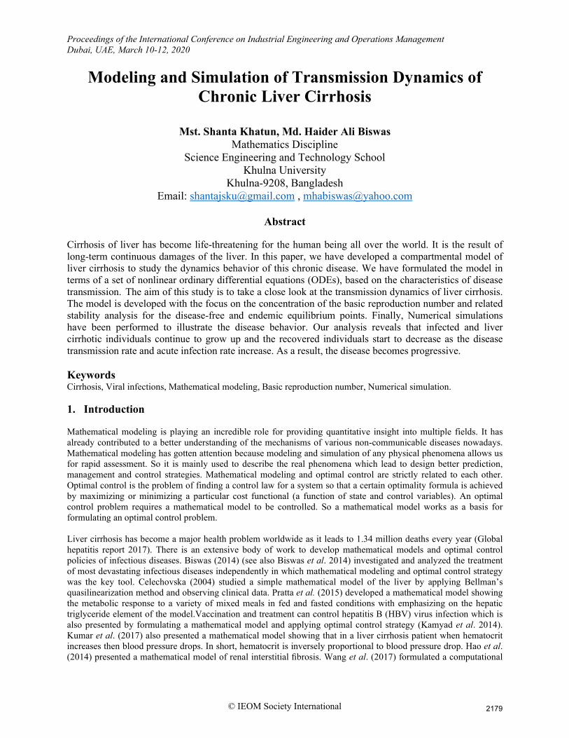
In the basic model, we assume that the population size is fixed ( )N t and the incubation period of the infectious agent is slowest. There are five compartments in the fundamental assumption of the compartmental model. The individuals who are not affected by infections like hepatitis B virus (HBV), hepatitis C virus (HCV) or by any kind of liver diseases. But they are prone to become affected by these infections or diseases. These populations are denoted by ( )S t

in the model. The disease transmission progress plays an important role in the dynamics of the

diseases. For most of the non-communicable diseases, there are always different ranges of the incubation period. The non-communicable disease liver cirrhosis is developed from long term progression of viral diseases, alcoholic disease, fatty liver disease or other liver diseases which were not diagnosed before in the body. The non-communicable disease liver cirrhosis is developed from long term progression of viral diseases such as hepatitis B (HBV) and hepatitis C (HCV) which were not diagnosed before in the body. These infections have a development period within the liver of the body. This incubation period of the infections usually ranges from approximately 10 to 15 years. So considering this, we have created another compartment called exposed individuals denoted by ( )E t .

Here, ( )E t is the number of infected individuals who are not infectious at time t. There are also some individuals

( )I t who are affected by infections (hepatitis B or hepatitis C) and can transmit at any time. When these infectionsremain undiagnosed for a long time, they become horrible. Long-time progression of these infections leads to cause cirrhosis. So we have considered the individuals ( )CL t who are affected by liver cirrhosis. The individuals who

have recovered and have the immunity from liver cirrhosis are denoted by ( )R t . Figure 6 shows the flowchart of thecompartmental model of liver cirrhosis.

2180



Figure 1. Flowchart of the compartmental model of liver cirrhosis.

Then taking all the situation into consideration, the liver cirrhosis model can be formulated by the following system of nonlinear ordinary differential equations:

( )

0

0

0

0

0

( )

( )

( )

c

c

cc

c

dS r I L S SdtdE I L S E EdtdI E I IdtdL

I p I Ldt

dR L I R p Idt

α σ µ

α σ µ β

β µ µ γ

µ γ µ δ ε

δ γ µ γ

= − + −

= + − −

= − − +

= + − + +

= + − −

( )1

with the boundary conditions ( ) ( ) ( ) ( ) ( )0 0 0 0 00 0, 0 0, 0 0, 0 0, 0 0c cS S E I I I L L R R= ≥ = ≥ = ≥ = ≥ = ≥ .

3. Analysis of the Model without Control We inquire the boundedness of solutions of the model, find out different equilibria (disease free and endemic equilibrium points), determine the basic reproduction number and perform the stability analysis at equilibria. 3.1. Boundedness of Solutions, Basic Reproduction Number and Equilibrium Points

Lemma 1: The region ( ) 5

0

, , , , /c crS E I L R S E I L Rµ+

Ω = ∈ + + + + ≤

is a positively invariant set for model (1).

Proof: Let, ( ) ( ) ( ) ( ) ( ) ( )cN t S t E t I t L t R t= + + + + . So, 0 cdN r N Ldt

µ ε= − − 0r Nµ≤ − , integrating and taking

limsup as t →∞ we get ( )0

limsupt

rN tµ→∞

≤ . Hence the Lemma 1 is proved.

In order to find disease free equilibrium point we have to solve 0cdLdS dE dI dRdt dt dt dt dt

∗∗ ∗ ∗ ∗

= = = = = . So, the model

(1) has the equilibrium point 0 0

0

( , , , , ) ,0,0,0,0crP S E I L R Pµ

∗ ∗ ∗ ∗ ∗ =

at which there is no infection. Therefore, the

2181



model (1) has a basic reproduction number 30

0 1 2 0 1 2 4

rrRαβ σϕαβ

µ ϕ ϕ µ ϕ ϕ ϕ= + . The basic reproduction number is performed

by next generation matrix method [8]. Again, * * *( , , , , )cP S E I L R∗ ∗ is the endemic equilibrium point of the model (1),

where 1 2 4

4 3

S ϕ ϕ ϕαβϕ αβσϕ

∗ =+

, ( )( )

4 3 0 1 2 4

1 4 3

rE

αβϕ αβσϕ µ ϕ ϕ ϕϕ αβϕ αβσϕ

∗ + +=

+, ( )

( )0 1 2 4 0 0 1 2 4

2 1 4 3

2 1RI

µ ϕ ϕ ϕ µ ϕ ϕ ϕβϕ ϕ αβϕ αβσϕ

∗ + −= +

,

( )( )

0 1 2 4 0 0 1 2 43

2 4 1 4 3

2 1c

RL

µ ϕ ϕ ϕ µ ϕ ϕ ϕβϕϕ ϕ ϕ αβϕ αβσϕ

∗ + −= +

and ( ) ( ) 0 3 43 4

0 1 2 4 4 3

1 pr p rR

µ β δϕ µ γ ϕδβϕ µ γ β ϕµ ϕ ϕ ϕ αβϕ αβσϕ

∗ + −−

= + +

.

3.2. Stability Analysis at Disease-free Equilibrium Point Now we perform stability analysis of the disease-free point by proving Theorem 1. Theorem 1: If 0 1R < then the disease free equilibrium point 0P of the model (1) is locally asymptotically stable and if 0 1R > then the disease free equilibrium point is unstable.

Proof: The Jacobian matrix of model (1) at the disease-free equilibrium point 0

,0,0,0,0rµ

is

( )

00 0

10 0

2

3 4

0

0 0

0 0

0 0 00 0 00 0

r r

r rJ

p

α ασµµ µα ασϕµ µ

β ϕϕ ϕµ γ δ µ

− − −

− = −

− − −

( )3

The characteristic equation is ( )2 3 20 0 1 2 3 0a a a aµ λ λ λ λ + + + + = , where 0 1 0a = > , 1 1 2 4 0a ϕ ϕ ϕ= + + > ,

( ) 32 1 4 2 4 1 2 0

0 4

1r

a Rαβ σϕ

ϕ ϕ ϕ ϕ ϕ ϕµ ϕ

= + + − + , and ( )3 1 2 4 01a Rϕ ϕ ϕ= − . According to the Routh-Hurwitz criterion, if

0 1R < then the eigenvalues of the characteristic equation have negative real parts. Hence, the Theorem 1 is proved. 3.3. Stability Analysis at Endemic Equilibrium Point Now we perform stability analysis of the endemic equilibrium point by proving Theorem 2. Theorem 2: If 0 1R > then the endemic equilibrium point P of the model (1) is locally asymptotically stable and if

0 1R < then the endemic equilibrium point is unstable. Proof: The Jacobian matrix of model (1) at the endemic equilibrium point is

( )

( )

0 1

1* * *

2

3 4

0

0 0 0( ) 0

0 0 0, , , ,0 0 00 0 1

c

c

I L S SJ S E I L R

p

µ ϕα σ ϕ α ασ

β ϕϕ ϕ

γ δ µ

∗ ∗ ∗ ∗

∗ ∗

− − + − −=

− − −

( )4

The matrix in equation (4) is a 5 5× matrix and the characteristic polynomial for the eigenvalue λ is given below, ( )det 0J Iλ− = ( )5

2182



( )

0 1

1

2

3 4

0

0 0 0( ) 0

0 0 0 00 0 00 0 1

cI L S S

p

µ λ ϕα σ ϕ λ α ασ

β ϕ λϕ ϕ λ

γ δ µ λ

∗ ∗ ∗ ∗

− − − + − − − −⇒ =

− − − − −

( )6

The characteristic equation is ( ) 4 3 20 0 1 2 3 4 0a a a a aµ λ λ λ λ λ − − + + + + = , where one eigenvalue of the

characteristic equation is 0λ µ= − which is negative. Again if 0 1R > , then it is clear that 2 3 4, , 0a a a > . Since

1 2 3, , ,a a a and 4a are same sign so according to Routh-Hurwitz criteria the other eigenvalues have negative real part. Again if 0 1R < , then at least one eigenvalue has positive real part. Therefore, the endemic equilibrium P is locally asymptotically stable if 0 1R > and unstable if 0 1R < . Hence, the Theorem 2 is proved. 4. Results and Discussion Numerical simulations of the proposed model (1) have been performed by the ODE45-solver using MATLAB programming. To solve the epidemic model, we have considered the initial values as 5.54,S = 0,E = 0.1,I =

0.3CL = , 0.2R = and all the parameters showed in Table 1. Our aim is to study the effects of two parameters i.e. transmission rate α of liver cirrhosis infection from susceptible to exposed individual compartment and acute infection rate β at which exposed individual entering into infected individual. The model has been simulated with the time of 20 years. Firstly, we have solved the model (1) for the tabulated values in Table 1 representing the initial and parametric values considered for our model. The simulations of the populations are shown in Figure 2-12.

Table 1: Parameter specifications of model (1)

Descriptions Parameters Values Source rate of susceptible population r 0.0121

Natural population death rate 0µ 0.95 Transmission rate α 0.16

Infectiousness of liver cirrhosis relative to acute infections σ 0.00693 Acute infection rate β 6 (per year)

Spontaneous recovery rate µ 0.25 Rate of moving from infection to liver cirrhosis γ 4 (per year)

Recovered rate from liver cirrhosis δ 0.03 Disease induced death rate ε 0.02

Rate of moving from recover to liver cirrhosis carriers p 0.25

2183



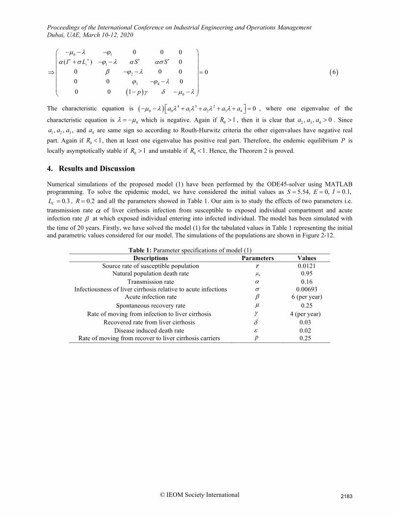
Figure 2. The disease behaviour of different individuals sizes in absence of control measures.

Figure 2 shows the state trajectories of the five compartments such as susceptible, exposed, infected, liver cirrhotic

and recovered individuals in the absence of any control measures. We have observed that when no control measure

is employed, the susceptible individual decreases from the initial state. The exposed individual increases initially but

about one and half years later the individual decreases and reduces to zero. The infected individuals also increase

and after 2 years it reduces. At the same time, the liver cirrhotic individuals increase from the initial state but after 3

years later the individuals drastically decrease. The recovered individuals gradually increase from the initial position

and reaches to the peak level.

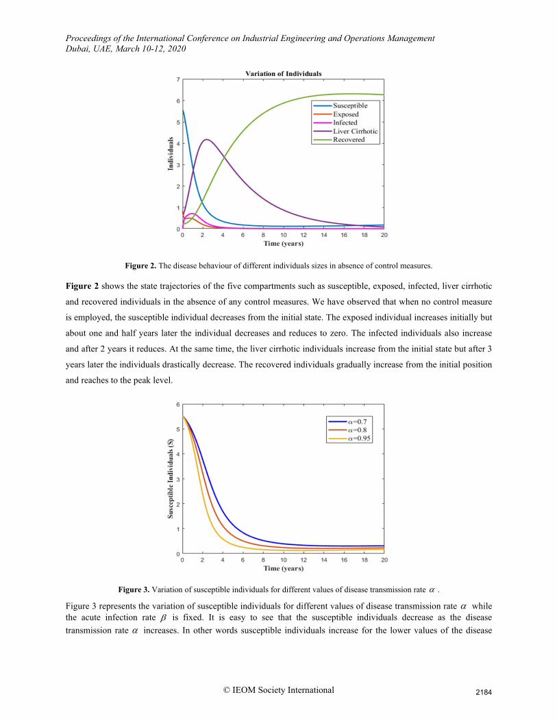
Figure 3. Variation of susceptible individuals for different values of disease transmission rate α .

Figure 3 represents the variation of susceptible individuals for different values of disease transmission rate α while the acute infection rate β is fixed. It is easy to see that the susceptible individuals decrease as the disease transmission rate α increases. In other words susceptible individuals increase for the lower values of the disease

2184



transmission rate α among the susceptible and exposed individuals. So that, those innumerable numbers of susceptible individuals are advancing to the exposed population for horizontal transmission.

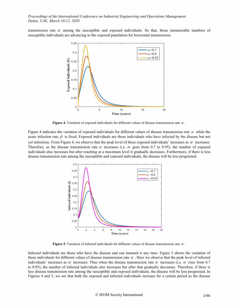
Figure 4. Variation of exposed individuals for different values of disease transmission rate α .

Figure 4 indicates the variation of exposed individuals for different values of disease transmission rate α while the acute infection rate β is fixed. Exposed individuals are those individuals who have infected by the disease but not yet infectious. From Figure 4, we observe that the peak level of these exposed individuals’ increases as α increases. Therefore, as the disease transmission rate α increases (i.e. α goes from 0.7 to 0.95), the number of exposed individuals also increases but after reaching at a maximum level it gradually decreases. Furthermore, if there is less disease transmission rate among the susceptible and exposed individuals, the disease will be less progressed.

Figure 5. Variation of infected individuals for different values of disease transmission rate α .

Infected individuals are those who have the disease and can transmit it any time. Figure 5 shows the variation of these individuals for different values of disease transmission rate α . Here we observe that the peak level of infected individuals’ increases as α increases. Thus when the disease transmission rate α increases (i.e. α rises from 0.7 to 0.95), the number of infected individuals also increases but after that gradually decreases. Therefore, if there is less disease transmission rate among the susceptible and exposed individuals, the disease will be less progressed. In Figures 4 and 5, we see that both the exposed and infected individuals increase for a certain period as the disease

2185



transmission rate α increases but it is noticeable that the number of infected individuals decreases more rapidly than the exposed individuals.

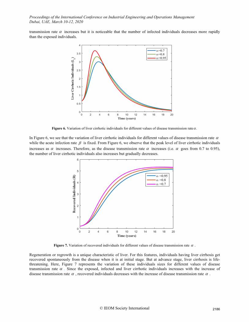
Figure 6. Variation of liver cirrhotic individuals for different values of disease transmission rate .α

In Figure 6, we see that the variation of liver cirrhotic individuals for different values of disease transmission rate α while the acute infection rate β is fixed. From Figure 6, we observe that the peak level of liver cirrhotic individuals increases as α increases. Therefore, as the disease transmission rate α increases (i.e. α goes from 0.7 to 0.95), the number of liver cirrhotic individuals also increases but gradually decreases.

Figure 7. Variation of recovered individuals for different values of disease transmission rate α .

Regeneration or regrowth is a unique characteristic of liver. For this features, individuals having liver cirrhosis get recovered spontaneously from the disease when it is at initial stage. But at advance stage, liver cirrhosis is life-threatening. Here, Figure 7 represents the variation of these individuals sizes for different values of disease transmission rate α . Since the exposed, infected and liver cirrhotic individuals increases with the increase of disease transmission rate α , recovered individuals decreases with the increase of disease transmission rate α .

2186



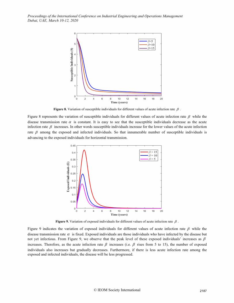
Figure 8. Variation of susceptible individuals for different values of acute infection rate β .

Figure 8 represents the variation of susceptible individuals for different values of acute infection rate β while the disease transmission rate α is constant. It is easy to see that the susceptible individuals decrease as the acute infection rate β increases. In other words susceptible individuals increase for the lower values of the acute infection rate β among the exposed and infected individuals. So that innumerable number of susceptible individuals is advancing to the exposed individuals for horizontal transmission.

Figure 9. Variation of exposed individuals for different values of acute infection rate β .

Figure 9 indicates the variation of exposed individuals for different values of acute infection rate β while the disease transmission rate α is fixed. Exposed individuals are those individuals who have infected by the disease but not yet infectious. From Figure 9, we observe that the peak level of these exposed individuals’ increases as β increases. Therefore, as the acute infection rate β increases (i.e. β rises from 5 to 15), the number of exposed individuals also increases but gradually decreases. Furthermore, if there is less acute infection rate among the exposed and infected individuals, the disease will be less progressed.

2187



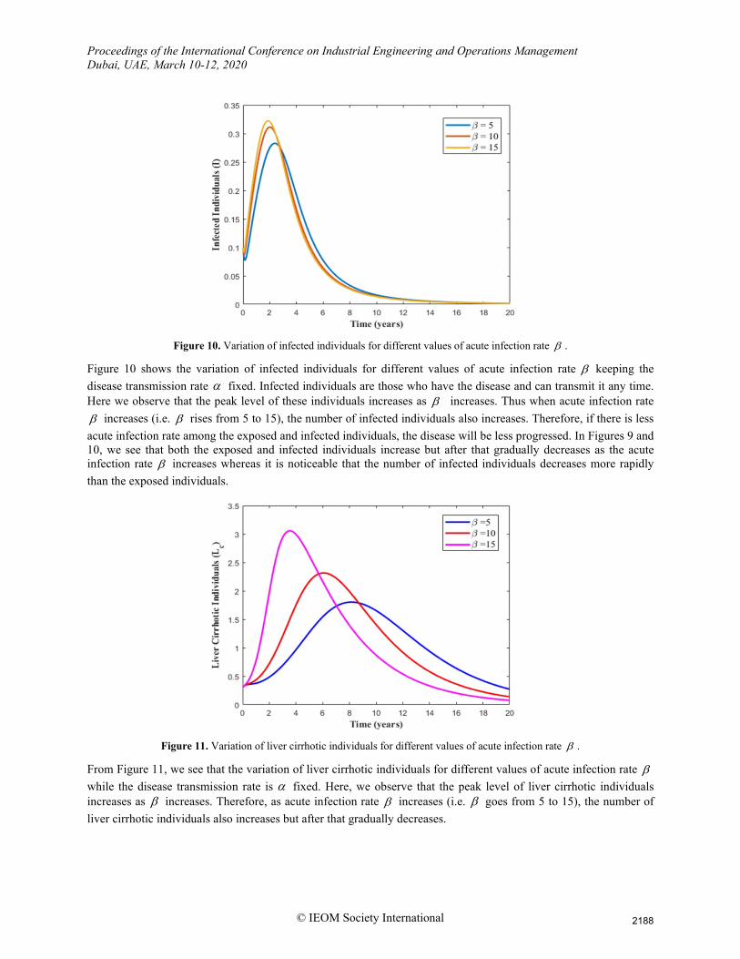
Figure 10. Variation of infected individuals for different values of acute infection rate β .

Figure 10 shows the variation of infected individuals for different values of acute infection rate β keeping the disease transmission rate α fixed. Infected individuals are those who have the disease and can transmit it any time. Here we observe that the peak level of these individuals increases as β increases. Thus when acute infection rate β increases (i.e. β rises from 5 to 15), the number of infected individuals also increases. Therefore, if there is less acute infection rate among the exposed and infected individuals, the disease will be less progressed. In Figures 9 and 10, we see that both the exposed and infected individuals increase but after that gradually decreases as the acute infection rate β increases whereas it is noticeable that the number of infected individuals decreases more rapidly than the exposed individuals.

Figure 11. Variation of liver cirrhotic individuals for different values of acute infection rate β .

From Figure 11, we see that the variation of liver cirrhotic individuals for different values of acute infection rate β while the disease transmission rate is α fixed. Here, we observe that the peak level of liver cirrhotic individuals increases as β increases. Therefore, as acute infection rate β increases (i.e. β goes from 5 to 15), the number of liver cirrhotic individuals also increases but after that gradually decreases.

2188



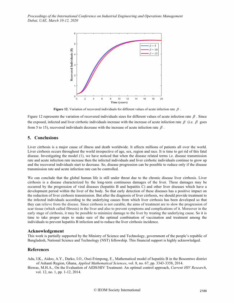
Figure 12. Variation of recovered individuals for different values of acute infection rate β .

Figure 12 represents the variation of recovered individuals sizes for different values of acute infection rate β . Since the exposed, infected and liver cirrhotic individuals increase with the increase of acute infection rate β (i.e. β goes from 5 to 15), recovered individuals decrease with the increase of acute infection rate β . 5. Conclusions Liver cirrhosis is a major cause of illness and death worldwide. It affects millions of patients all over the world. Liver cirrhosis occurs throughout the world irrespective of age, sex, region and race. It is time to get rid of this fatal disease. Investigating the model (1), we have noticed that when the disease related terms i.e. disease transmission rate and acute infection rate increase then the infected individuals and liver cirrhotic individuals continue to grow up and the recovered individuals start to decrease. So, disease progression can be possible to reduce only if the disease transmission rate and acute infection rate can be controlled. We can conclude that the global human life is still under threat due to the chronic disease liver cirrhosis. Liver cirrhosis is a disease characterized by the long-term continuous damages of the liver. These damages may be occurred by the progression of viral diseases (hepatitis B and hepatitis C) and other liver diseases which have a development period within the liver of the body. So that early detection of these diseases has a positive impact on the reduction of liver cirrhosis transmission. But after the diagnosis of liver cirrhosis, we should provide treatment to the infected individuals according to the underlying causes from which liver cirrhosis has been developed so that they can relieve from the disease. Since cirrhosis is not curable, the aims of treatment are to slow the progression of scar tissue (which called fibrosis) in the liver and also to prevent symptoms and complications of it. Moreover in the early stage of cirrhosis, it may be possible to minimize damage to the liver by treating the underlying cause. So it is time to take proper steps to make sure of the optimal combination of vaccination and treatment among the individuals to prevent hepatitis B infection and to reduce the liver cirrhosis incidence. Acknowledgement This work is partially supported by the Ministry of Science and Technology, government of the people’s republic of Bangladesh, National Science and Technology (NST) fellowship. This financial support is highly acknowledged. References Adu, I.K., Aidoo, A.Y., Darko, I.O., Osei-Frimpong, E., Mathematical model of hepatitis B in the Bosomtwe district

of Ashanti Region, Ghana, Applied Mathematical Sciences, vol. 8, no. 67, pp. 3343-3358, 2014. Biswas, M.H.A., On the Evaluation of AIDS/HIV Treatment: An optimal control approach, Current HIV Research,

vol. 12, no. 1, pp. 1-12, 2014.

2189



Biswas, M.H.A., Paiva L.T. and de Pinho, M.D.R., A SEIR model for control of infectious diseases with constraints, Mathematical Biosciences and Engineering, vol. 11, no. 4, pp. 761-784, 2014.

Celechovska L., A simple mathematical model of the human liver, Applications of Mathematics, vol. 49, no. 3, pp. 227-246, 2004.

Global hepatitis report 2017, World Health Organization (WHO), 2017, Switzerland, Geneva. Greena, J.E.F., Watersa, S.L., Shakesheff, K.M., and Byrne, H.M. A, Mathematical model of liver cell aggregation

in vitro, Bulletin of Mathematical Biology, vol. 71, no. 4, pp. 906-930, 2009. Huwart, L., Peeters, F., Sinkus, R., Annet, L., Salameh, N., Beek, L.C., Horsmans, Y. and Beers, B.E.V., liver

fibrosis: non-invasive assessment with MR elastography, NMR in biomedicine, vol. 19, pp. 173-179, 2006. Hao, W., Rovin, B.H. and Friedman, A., Mathematical model of renal interstitial fibrosis, Proceedings of the National Academy of Sciences of the United States of America, vol. 111, no. 39, pp. 14193-14198, 2014.

Kumar, A., Upadhyay, V., Agrawal, A.K. and Pandey, P.N., A mathematical modeling of two phase hepatic mean blood flow in arterioles during liver cirrhosis, International Journal of Applied Research, vol. 3, no. 7, pp. 506-507, 2017.

Kamyad, A.V., Akbari, R., Heydari, A.A. and Heydari, A., Mathematical modeling of transmission dynamics and optimal control of vaccination and treatment for hepatitis B virus, Computational and Mathematical Methods in Medicine, vol. 2014, pp. 1-15, 2014.

Khatun, M.S. and Biswas, M.H.A., Modeling the effect of adoptive T cell therapy for the treatment of leukemia. Computational and Mathematical Methods, doi: 10.1002/cmm4.1069, 2019.

Momoh, A.A., Ibrahim, M.O., Madu, B.A. and Asogwa, K.K., Stability analysis of mathematical model of hepatitis B, Current Research Journal of Biological Sciences, vol. 4, no. 5, pp. 534-537, 2012.

Pratt, A.C., Wattis, J.A.D., and Salter, A.M., Mathematical modeling of hepatic lipid metabolism, Mathematical Bioscience, vol. 262, no. 2015, pp. 167-181, 2015.

Remien, C.H., Adler F.R., Waddoups, L., Box, T.D., and Sussman, N.L., Mathematical modeling of liver injury and dysfunction after acetaminophen overdose: early discrimination between survival and death, Hepatology, vol. 56, no. 2, pp. 227-234, 2012.

Wang, T., Liang, F., Jhou, J., and Shi, L., A computational model of the hepatic circulation applied to analyze the sensitivity of hepatic venous pressure gradient (HVPG) in liver cirrhosis, Journal of Biomechanics, vol. 65, pp. 23-31, 2017.

Biographies Mst. Shanta Khatun has recently completed her M.Sc in applied Mathematics from Khulna University, Khulna-9208, Bangladesh under Science Engineering and Technology School. She completed her Bachelor of Science (Honors) degree in Mathematics in the year 2017 from the same University. She Attended CIMPA (International Centre for Pure and Applied Mathematics) research school on Dynamical Systems and its Applications to Biology during June 10-21, 2019 in the Department of Mathematics held at University of Dhaka. Her research interests include Mathematical Modeling and Simulations, Biomathematics, and Epidemiology of Chronic Diseases. Dr. Haider Ali Biswas is currently affiliated with Khulna University, Bangladesh as a Professor of Mathematics under Science Engineering and Technology School. Prof. Biswas obtained his B. Sc. (Honors) in Mathematics and M.Sc in Applied Mathematics in the year 1993 and 1994 respectively from the University of Chittagong, Bangladesh, M Phil in Mathematics in the year 2008 from the University of Rajshahi, Bangladesh and PhD in Electrical and Computer Engineering from the University of Porto, Portugal in 2013. He has more than 18 years teaching and research experience in the graduate and postgraduate levels at different public universities in Bangladesh. He published three books, one chapters and more than 70 research papers in the peer reviewed journals and international conferences. His present research interests include Optimal Control with State Constraints, Nonsmooth Analysis, Mathematical Modeling and Simulation, Mathematical Biology and Biomedicine, Epidemiology of Infectious Diseases. Recently Professor Biswas has been nominated the Member of the Council of Asian Science Editors (CASE) for 2017-2020 and the Associate Member of the Organization for Women in Science for the Developing World (OWSD) since 2017.

2190

https://www.sciencedirect.com/science/journal/00255564/262/supp/C

modeling and simulation of transmission dynamics of

Documents